STATISTICAL APPLICATIONS IN PLANT BREEDING AND ...
135
STATISTICAL APPLICATIONS IN PLANT BREEDING AND GENETICS By CARL ALAN WALKER A dissertation submitted in partial fulfillment of the requirements for the degree of DOCTOR OF PHILOSOPHY IN CROP SCIENCE WASHINGTON STATE UNIVERSITY Department of Crop and Soil Sciences MAY 2012
-
Upload
khangminh22 -
Category
Documents
-
view
0 -
download
0
Transcript of STATISTICAL APPLICATIONS IN PLANT BREEDING AND ...

STATISTICAL APPLICATIONS IN PLANT BREEDING
AND GENETICS
By
CARL ALAN WALKER
A dissertation submitted in partial fulfillment of
the requirements for the degree of
DOCTOR OF PHILOSOPHY IN CROP SCIENCE
WASHINGTON STATE UNIVERSITY
Department of Crop and Soil Sciences
MAY 2012

ii
To the Faculty of Washington State University:
The members of the Committee appointed to examine the dissertation of CARL ALAN
WALKER find it satisfactory and recommend that it be accepted.
Kimberly Garland-Campbell, Ph.D., Chair
Fabiano Pita, Ph.D.
J. Richard Alldredge, Ph.D.
Richard Gomulkiewicz, Ph.D.
Daniel Skinner, Ph.D.

iii
ACKNOWLEDGEMENT
I would like to thank my committee members for their advice and assistance with this research
and with writing this dissertation. I would like to thank all the members of both the Campbell
and Steber labs for their advice when I presented my work in lab meetings. I began the project
presented in Chapter 3 as part of a paid internship with Dow AgroSciences. I would like to
thank the members of the Dow AgroSciences Quantitative Genetics group for their assistance
during that internship, especially Kelly Robins who provided some initial programs and data. I
would also like to acknowledge Bruce Walsh, Rebecca Doerge, and Radu Totir for the valuable
advice they gave me at conferences where I presented my work. I would not have been able conduct
this research without the funding for these projects by the Washington Grain Commission and
USDA project 5348-21000-023-00. Finally I‟d like to thank my parents for all their help getting
me this far and my wife Elizabeth for her help editing and moral support.

iv
STATISTICAL APPLICATIONS IN PLANT BREEDING AND
GENETICS
ABSTRACT
by Carl Alan Walker, Ph.D.
Washington State University
May 2012
Chair: Kimberly Garland-Campbell
Statistical analysis has many applications ensuring the validity and reproducibility of plant
breeding and genetics research. Crop plant germplasm collections are often too large to be of use
regularly. A core subset with fewer accessions can increase utility while maintaining most of the genetic
diversity of the complete collection. This study evaluated methods for selecting core subsets using sparse
data. Cores were selected by forming clusters of accessions based on distances estimated with phenotypic
data. Accessions were randomly selected relative to the number of accessions in each cluster. The
method using all the available data to calculate distances, average linkage clustering, and
sampling in proportion to the natural logarithm of cluster size produced the most diverse cores.
Evaluations of genotypes in varied environmental conditions are referred to as multiple
environment trials (MET) and often necessitate estimation of effects of genotypes within environments.
Empirical best linear unbiased predictions can provide more accurate estimates of these effects,
depending upon the mixed model used. An objective of this work was to simulate and analyze MET data
sets to determine which models provide the most accurate estimates in varied MET conditions. Simulated
MET were fit with mixed models with or without genetic relationship matrices (GRM) and with
structures of varying complexity used to model relationships among environments. The model that
included a GRM and a constant variance-constant correlation structure was the most accurate for the

v
largest number of scenarios. More complex models were the most effective for a smaller subset of
scenarios, most involving many genotypes and low experimental error.
Statistical analyses were applied in consultation with other researchers for two projects
studying Fusarium crown rot of wheat and one on cold tolerance of wheat. Heritability and
genetic correlations were calculated for Fusarium resistance assays in field, growth chamber, and
terrace bed settings. Factor analysis was used to estimate latent factors from field characteristic
variables, which were used as predictor variables in linear mixed models and generalized linear
mixed models. Cold tolerance among genotypes was assessed with logistic regression.

vi
TABLE OF CONTENTS
ACKNOWLEDGEMENT ........................................................................................................ III
ABSTRACT .............................................................................................................................. IV
TABLE OF CONTENTS .......................................................................................................... VI
LIST OF TABLES .................................................................................................................... IX
LIST OF FIGURES .................................................................................................................... X
LITERATURE REVIEW ............................................................................................................... 1
CORE SUBSETS OF GERMPLASM COLLECTIONS ........................................................................... 1
MIXED MODELS FOR MULTIPLE ENVIRONMENT TRIALS ............................................................. 6
HERITABILITY AND GENETIC CORRELATION ............................................................................. 13
DIMENSION REDUCTION FOR LINEAR MODELING ..................................................................... 17
EXTREME COLD TOLERANCE IN WHEAT ................................................................................... 20
REFERENCES ............................................................................................................................. 22
METHODS FOR SELECTING GERMPLASM CORE SUBSETS USING SPARSE
PHENOTYPIC DATA.................................................................................................................. 30
ABSTRACT ................................................................................................................................. 30
INTRODUCTION.......................................................................................................................... 32
MATERIALS AND METHODS ...................................................................................................... 36
RESULTS ................................................................................................................................... 42
DISCUSSION .............................................................................................................................. 44
Conclusion ........................................................................................................................ 47
APPENDIX ................................................................................................................................. 47

vii
REFERENCES ............................................................................................................................. 50
COMPARISON OF LINEAR MIXED MODELS FOR MULTIPLE ENVIRONMENT PLANT
BREEDING TRIALS ................................................................................................................... 64
ABSTRACT ................................................................................................................................. 64
INTRODUCTION.......................................................................................................................... 65
METHODS .................................................................................................................................. 68
Simulations ....................................................................................................................... 68
Analyses ............................................................................................................................ 70
RESULTS AND DISCUSSION ........................................................................................................ 74
Justification of Approach .................................................................................................. 74
Choice of a Default Model ................................................................................................ 75
Models for Specific Scenarios .......................................................................................... 76
DISCUSSION .............................................................................................................................. 78
Conclusions ....................................................................................................................... 80
APPENDIX: REAL DATA AS A BASIS FOR SIMULATIONS ............................................................. 81
REFERENCES ............................................................................................................................. 83
CONSULTING PROJECTS ......................................................................................................... 98
HERITABILITY AND GENETIC CORRELATION ANALYSES FOR FUSARIUM CROWN ROT
RESISTANCE ASSAYS OF WHEAT MAPPING POPULATION .......................................................... 98
Abstract ................................................................................................................................. 98
Discussion of Statistical Methods ......................................................................................... 99
LINEAR MODELING OF THE RELATIONSHIPS BETWEEN WHEAT FIELD CHARACTERISTICS AND
FUSARIUM CROWN ROT OBSERVATIONS ................................................................................. 106

viii
Abstract ............................................................................................................................... 106
Discussion of Statistical Methods ....................................................................................... 107
LOGISTIC REGRESSION ANALYSIS OF WHEAT COLD TOLERANCE TESTING ............................ 112
Summary ............................................................................................................................. 112
Discussion of Methods ........................................................................................................ 113
REFERENCES ........................................................................................................................... 120

ix
LIST OF TABLES
Table 1. Measurement levels and missing value percentages of variables evaluated on the
Triticum aestivum L. subsp. aestivum complete collection. ......................................................... 54
Table 2. Removal percentages by variable for simulating data sets with missing values
by removing values from the "complete collection". .................................................................... 55
Table 3. Comparisons of core subset selection methods in terms of diversity of 1000
potential core subsets selected from 200 complete collections simulated with values removed at
the rates given by set 1 (see Table 2) from accessions selected randomly from a uniform
distribution. ................................................................................................................................... 56
Table 4. Comparisons of core subset selection methods in terms of diversity of 1000
potential core subsets selected from 200 complete collections simulated with values removed at
the rates given by set 1 (see Table 2) from accessions selected as a contiguous group. .............. 57
Table 5. Comparisons of core subset selection methods in terms of diversity of 1000
potential core subsets selected from 200 complete collections simulated with values removed at
the rates given by set 2 (see Table 2) from accessions selected randomly from a uniform
distribution. ................................................................................................................................... 58
Table 6. Comparisons of core subset selection methods in terms of diversity of 1000
potential core subsets selected from 200 complete collections simulated with values removed at
the rates given by set 2 (see Table 2) from accessions selected as a contiguous group. .............. 59

x
LIST OF FIGURES
Figure 1. Plot of cumulative means, over simulations, of median recovery of interquartile
range, over 1000 potential core subsets per simulation. Simulations were generated by removing
values from randomly chosen individual accessions with missingness rates given by set 1. The
values of the means of all 200 simulations are shown in Table 3……………………………..…60
Figure 2. Plot of cumulative means, over simulations, of median recovery of interquartile
range, over 1000 potential core subsets, ranked across methods within each simulation.
Simulations were generated by removing values from randomly chosen individual accessions
with missingness rates given by set 1. The mean ranks, over all 200 simulations, are shown in
Table 3.…………………………………………………………………………………………..61
Figure 1. Means, over simulations, of model ranks, where models were ranked in terms
of RMSEP within each simulation. All scenarios evaluated are included, and index denotes each
scenario‟s position in the order. Scenarios are ordered CSA, CSAH, CSAVH, CSB, CSBH,
CSBVH, Toep, ToepH, and then ToepVH, with the indices of the final scenarios of each group
equal to 76, 154, 230, 304, 380, 456, 532, 608, and 682, respectively. Within each of these
patterns, numbers of environments are ordered 5, 10, 20, and then 40 environments. Within each
number of environments, the numbers of genotypes are ordered 25, 50, 100, and then 150
genotypes. Within each number of genotypes, the experimental designs are ordered RCBD,
MAD, and then unreplicated designs. Within each design, error variances are ordered 0.5 then
2.0.……………………………………………………………………………………………..…85
Figure 2. A standardized version of Figure 1, where models have been ranked within
each scenario in terms of their mean ranks. The order of scenarios is the same as Figure 1…...86

xi
Figure 3. The same as figure 2, but only the models GRM_CorV and GRM_CorH. The
order of scenarios is the same………………………………………………………..……..……87
Figure 4. Equivalent to Figure 3, with only scenarios with high (2.0) error variance
included. Scenarios are ordered CSA, CSAH, CSAVH, CSB, CSBH, CSBVH, Toep, ToepH, and
then ToepVH, with the indices of the final scenarios of each group equal to 39, 78, 116, 154,
192, 230, 268, 306, and 343, respectively. Within each of these patterns, numbers of
environments are ordered 5, 10, 20, and then 40 environments. Within each number of
environments, the numbers of genotypes are ordered 25, 50, 100, and then 150 genotypes.
Within each number of genotypes, the experimental designs are ordered RCBD, MAD, and then
unreplicated designs.……………………………………………………………………….….....88
Figure 5. Equivalent to Figure 3, with only scenarios with low (0.5) error variance
included. Scenarios are ordered CSA, CSAH, CSAVH, CSB, CSBH, CSBVH, Toep, ToepH, and
then ToepVH, with the indices of the final scenarios of each group equal to 37, 76, 114, 150,
188, 226, 264, 302, and 339, respectively. Within each of these patterns, numbers of
environments are ordered 5, 10, 20, and then 40 environments. Within each number of
environments, the numbers of genotypes are ordered 25, 50, 100, and then 150 genotypes.
Within each number of genotypes, the experimental designs are ordered RCBD, MAD, and then
unreplicated designs.……………………………………………………………………………..89
Figure 6. Equivalent to Figure 3, only including scenarios simulated with a compound
symmetric pattern of relationships among environments. Scenarios are ordered CSA, then CSB,
with the indices of the final scenarios of each group equal to 76 and 150, respectively. Within
each of these patterns, numbers of environments are ordered 5, 10, 20, and then 40 environments.
Within each number of environments, the numbers of genotypes are ordered 25, 50, 100, and

xii
then 150 genotypes. Within each number of genotypes, the experimental designs are ordered
RCBD, MAD, and then unreplicated designs. Within each design, error variances are ordered
0.5 then 2.0.……………………………………………………………..……………….……….90
Figure 7. Equivalent to Figure 3, only including scenarios simulated with a compound
symmetric pattern of correlations among environments and heterogeneous variances of genotype
effects within environments. Scenarios are ordered CSAH, then CSBH, with the indices of the
final scenarios of each group equal to 78 and 154, respectively. Within each of these patterns,
numbers of environments are ordered 5, 10, 20, and then 40 environments. Within each number
of environments, the numbers of genotypes are ordered 25, 50, 100, and then 150 genotypes.
Within each number of genotypes, the experimental designs are ordered RCBD, MAD, and then
unreplicated designs. Within each design, error variances are ordered 0.5 then 2.0.……..……91
Figure 8. Equivalent to Figure 3, only including scenarios simulated with a compound
symmetric pattern of correlations among environments and extremely heterogeneous variances
of genotype effects within environments. Scenarios are ordered CSAVH, then CSBVH, with the
indices of the final scenarios of each group equal to 76 and 152, respectively. Within each of
these patterns, numbers of environments are ordered 5, 10, 20, and then 40 environments.
Within each number of environments, the numbers of genotypes are ordered 25, 50, 100, and
then 150 genotypes. Within each number of genotypes, the experimental designs are ordered
RCBD, MAD, and then unreplicated designs. Within each design, error variances are ordered
0.5 then 2.0.………………………………………….…………………………………….….…92
Figure 9. Equivalent to Figure 3, only including scenarios simulated with a Toeplitz
pattern of correlations among environments. Scenarios are ordered Toep, ToepH, and then
ToepVH, with the indices of the final scenarios of each group equal to 76, 152, and 226,

xiii
respectively. Within each of these patterns, numbers of environments are ordered 5, 10, 20, and
then 40 environments. Within each number of environments, the numbers of genotypes are
ordered 25, 50, 100, and then 150 genotypes. Within each number of genotypes, the
experimental designs are ordered RCBD, MAD, and then unreplicated designs. Within each
design, error variances are ordered 0.5 then 2.0.………………………………….……….….…93
Figure 10. Equivalent to Figure 3, only including scenarios simulated with a Toeplitz
pattern of correlations among environments, 100 or 150 genotypes, 5 to 20 environments, and
low (0.5) error variance. Scenarios are ordered Toep, ToepH, and then ToepVH, with the indices
of the final scenarios of each group equal to 14, 29, and 43, respectively. Within each of these
patterns, numbers of environments are ordered 5, 10, and then 20 environments. Within each
number of environments, the numbers of genotypes are ordered 100 and then 150 genotypes.
Within each number of genotypes, the experimental designs are ordered RCBD, MAD, and then
unreplicated designs.….……………………………………………………………………….…94
Figure 11. Equivalent to Figure 3, only including scenarios simulated with 25 genotypes.
Scenarios are ordered CSA, CSAH, CSAVH, CSB, CSBH, CSBVH, Toep, ToepH, and then
ToepVH, with the indices of the final scenarios of each group equal to 24, 48, 72, 96, 120, 144,
168, 192, and 216, respectively. Within each of these patterns, numbers of environments are
ordered 5, 10, 20, and then 40 environments. Within each number of environments, the
experimental designs are ordered RCBD, MAD, and then unreplicated designs. Within each
design, error variances are ordered 0.5 then 2.0.…………………………………..…..………..95
Figure 12. Equivalent to Figure 3, only including scenarios simulated with MAD or
unreplicated designs. Scenarios are ordered CSA, CSAH, CSAVH, CSB, CSBH, CSBVH, Toep,
ToepH, and then ToepVH, with the indices of the final scenarios of each group equal to 50, 102,

xiv
154, 203, 255, 307, 357, 409, and 461, respectively. Within each of these patterns, numbers of
environments are ordered 5, 10, 20, and then 40 environments. Within each number of
environments, the numbers of genotypes are ordered 25, 50, 100, and then 150 genotypes.
Within each number of genotypes, the experimental designs are ordered MAD, and then
unreplicated designs. Within each design, error variances are ordered 0.5 then 2.0.…………...96
Figure 13. A standardized version of Figure 1, where only models not including GRM
have been ranked within each scenario in terms of their mean ranks. The order of scenarios is
the same.………………………………………………………………………………......……..97

1
CHAPTER 1
LITERATURE REVIEW
Crop science research relies on statistical methods to assist in making objective decisions based on
complex and subtle patterns in nature that are not always obvious from raw observations or observed
results from experiments. Among other tasks in crop science research, statistical methods may be used to
group genotypes based on phenotypic data, make accurate predictions about the future performance of
breeding material, estimate relationships from observational data, and test hypotheses from designed
experiments.
Core Subsets of Germplasm Collections
Crop plant germplasm collections are maintained to conserve genetic variation and to provide useful plant
material for researchers and plant breeders. An example is the collection of wheat (Triticum aestivum L.
subsp. aestivum) accessions maintained as part of the National Small Grains Collection of the USDA-
ARS National Plant Germplasm System (http://www.ars-grin.gov/npgs/index.html).
For many researchers and plant breeders, germplasm collections are often too large and too
lacking in descriptive data to be of practical use. A well-characterized core collection, or core subset
(these terms will be used interchangeably), that consists of a reduced number of accessions (usually about
10% of the total) can provide increased accessibility and utility while still maintaining most of the genetic
diversity of the complete collection (Brown, 1989). Users of core subsets generally seek a diverse sample
that varies for one or more characteristics. For example, Wang et al. (2010) evaluated a rice core subset
for resistance to the blast fungal disease and identified known and novel genetic sources for resistance.
These researchers utilized the core subset to access the genetic diversity of the complete collection
without needing to evaluate the large numbers of very similar accessions held in the complete collection.
For desired alleles that are evenly distributed throughout the whole collection, at any level of abundance,
a simple random sample of the complete collection is the most appropriate. This is because every

2
accession selected for the core subset would have an equal chance of having the specific allele. If desired
alleles are instead localized to certain parts of the collection, preferentially selecting a portion from each
heterogeneous group present in the complete collection increases the likelihood of selecting these
unevenly distributed alleles (Brown, 1989). For this reason, most researchers have constructed core
collections by grouping accessions and then selecting accessions within groups.
A number of different methods and types of data have been used to group accessions and select
core collections. Passport data, i.e. the location of cultivation or collection, has been used to stratify the
complete collection, followed by selection from within each stratum. This technique was used to select a
core subset for the complete wheat collection described above (USDA ARS, National Genetic Resources
Program, 2009), and this method has also been used to develop other core collections (Skinner et al.,
1999; Huamán et al., 2000; Dahlberg et al., 2004; Yan et al., 2007). Other methods for selecting core
collections have included stratification based on geographic origin, followed by further grouping based on
cluster analysis of phenotypic traits (Basigalup et al., 1995; Rao and Rao, 1995; Igartua et al., 1998; Tai
and Miller, 2001; Upadhyaya et al., 2001, 2006; Mahalakshmi et al., 2006; Bhattacharjee et al., 2007;
Dwivedi et al., 2008). Stratification of collections has also been conducted using cluster analysis without
prior geographic grouping (Diwan et al., 1995; Franco et al., 1997, 1998, 1999, 2005; Grenier et al.,
2001a; Li et al., 2004; Anderson, 2005; Holbrook and Dong, 2005; Weihai et al., 2008; Upadhyaya et al.,
2008). A study which compared methods for selecting core subsets using relatively complete phenotypic
data demonstrated that selection based on clustering using those data was superior to selection based on
geographic origin alone (Diwan et al., 1995).
Researchers have also conducted cluster analysis based on genotypic data, either based on actual
genotyping (Franco et al., 2006; Wang et al., 2006; Balfourier et al., 2007; Escribano et al., 2008; Hao et
al., 2008) or predicted genotypic effects based on modeling of phenotypic data (Hu et al., 2000; Li et al.,
2004). Combinations of genotypic and phenotypic data have also been used to group accessions (Franco
et al., 2010). Grouping based on genotype data would be expected to better reflect the genetic
relationships among accessions. However, researchers are limited in the number of accessions that can be

3
evaluated and the depth of genotyping possible. Such limitations may prevent the selection of core
subsets from large collections based on genetic data or may result in cores that are not as diverse as those
selected based on non-genetic data
The clustering method used and the data used in the clustering process have also varied. Choice
of clustering method determines the way in which variable data or distance calculations are used to group
accessions and different method choices can result in dramatic differences in final grouping. Ward‟s
minimum variance method is one clustering method used by many researchers to construct cores (Franco
et al., 1997; Hu et al., 2000; Upadhyaya et al., 2006, 2008, 2001; Anderson, 2005; Holbrook and Dong,
2005; Reddy et al., 2005; Kang et al., 2006; Mahalakshmi et al., 2006; Bhattacharjee et al., 2007;
Dwivedi et al., 2008). Other clustering methods that have been used include unweighted pair-group
method using arithmetic average (UPGMA), also known as the average linkage method (Hu et al., 2000;
Huamán et al., 2000; Li et al., 2004; Franco et al., 2006; Weihai et al., 2008); complete linkage (Hu et al.,
2000); and the Ward-Modified Location Method (Franco et al., 1998, 1999, 2005). Authors have
constructed clusters based on a variety of phenotypic variables. In many cases these variables have been
uniformly quantitative, and authors often either used Euclidian distances or principle components to
determine relationships among accessions and construct clusters (Diwan et al., 1995; Igartua et al., 1998;
Holbrook and Dong, 2005; Kang et al., 2006; Bhattacharjee et al., 2007; Upadhyaya et al., 2008).
However, a smaller number of researchers have used both categorical and quantitative variables in cluster
analysis (Franco et al., 1997, 1998, 1999, 2005; Kroonenberg et al., 1997).
Grouping via geographic information and/or cluster analysis serves two purposes. The first is to
aid in selecting a core with reduced redundancy as described above. The second benefit of grouping is
that it provides structure to the accessions and connections to the reserve collection, which is the set of
accessions from the complete collection that are not included in the core. If breeders find lines in the core
collection that are of interest, they can trace connections from these lines to sets of additional accessions
in the reserve with similar characteristics. Ideally these accessions will be genetically similar to the
accessions in the core, although this will depend on the effectiveness of the grouping. Milkas et al.

4
(1999) reported using core and reserve collections of common bean in such a way to discover sources of
white mold resistance beyond a set found in a core subset.
Following the stratification and clustering of the complete collection, a set of accessions is chosen
from each group and compiled into a core. Generally accessions are chosen at random from each stratum;
however, some researchers have suggested that direct, or only partially random, selection of all or a
portion of the accessions in a core can increase diversity (Basigalup et al., 1995; Skinner et al., 1999;
Huamán et al., 2000; Rodiño et al., 2003; Yan et al., 2007; Weihai et al., 2008). Several core subsets
have been selected using proportional sampling, a random selection method that determines quantities of
accessions from each group in proportion to the number of accessions in each group (Basigalup et al.,
1995; Upadhyaya et al., 2001, 2006, 2008; Grenier et al., 2001b; Dahlberg et al., 2004; Holbrook and
Dong, 2005; Reddy et al., 2005; Bhattacharjee et al., 2007; Dwivedi et al., 2008). This proportional
sampling method is the most effective choice if the numbers of accessions in each group in the complete
collection perfectly reflect the true genetic diversity of all the genotypes in the world that could fit in that
group. In reality, the selection of accessions for germplasm collections may differ markedly from such
perfection, largely due to constraints on collection activities. Sampling methods that take relatively fewer
samples from larger clusters reduce redundancy and increase variability, as larger clusters tend to have
greater redundancy among accessions (Brown, 1989). Common implementations of such sampling
strategies include selection in proportion to the square root (Huamán et al., 2000; Wang et al., 2006) and
natural logarithm of group size (Grenier et al., 2001b; Yan et al., 2007). Selecting equal numbers of
accessions from each group, regardless of the size of the group, is the most extreme method for
attempting to reduce redundancy. Rather than basing sampling strategy on the relationships between
group sizes and diversity, some sampling methods attempt to increase diversity by selecting more
accessions from groups with greater relative diversity. An example of this is selecting sample numbers
relative to the mean distance among accessions in each cluster (Franco et al., 2005).
One aspect of the core collections developed in the studies referenced above is that they were
constructed using complete or nearly complete data sets of geographical, phenotypic, or genotypic data.

5
Unfortunately, many germplasm collections only have complete, or even mostly complete, data for a few
variables. Grouping based only on a few variables is unlikely to maintain the allelic diversity of genes
that affect other traits. Therefore, it is desirable to utilize all the variables for which we have even limited
information. One method for doing so is to use Gower‟s distance (Gower, 1971), as this metric allows the
calculation distances between accessions based on variables, of any measurement level (nominal, ordinal,
interval, or ratio), for which both accessions have values, and is not affected by variables for which either
accession has a missing value.
The goal of a core subset is to represent the diversity of a complete collection with a
reduced number of accessions. Therefore, the best method for selecting core subsets is the one
that results in the most diversity for a given number of accessions. A wide variety of tests and
calculations have been used to evaluate diversity of core subsets and to compare them to
complete collections under the assumption that core subsets and complete collections are
independent samples of some larger population. These methods have included chi-square tests
of independence of collection type and country of origin, marker alleles, and nominal phenotypic
variables (Tai and Miller, 2001; Upadhyaya et al., 2001, 2006, 2008; Grenier et al., 2001b;
Reddy et al., 2005; Mahalakshmi et al., 2006; Bhattacharjee et al., 2007; Agrama et al., 2009).
Differences between the distribution of quantitative variables for proposed core subsets and
complete collections have been tested using the Levene test and the Newman-Keuls test
(Upadhyaya et al., 2001, 2006, 2008; Grenier et al., 2001b; Reddy et al., 2005; Kang et al., 2006;
Bhattacharjee et al., 2007; Agrama et al., 2009). However, the validity of statistical tests of
differences between complete collections and core subsets is questionable, since these are not
independent samples in two respects. First, the complete collection is not a random sample of all
the germplasm for the species in the collection (due to limitations in collection activities), and so
statistics calculated on the complete collection should not be considered estimates of the

6
population of all germplasm for that species. Instead, the complete collection should be
considered a population of interest for which we can calculate exact parameter values. Second,
even if the complete collection is incorrectly considered a random sample, the core subset is not
independently sampled; it is a subset of the observations in the complete collection, violating an
assumption of these inference tests.
Aside from proper statistical testing, the other consideration when evaluating core subsets
is how distributions of variables in the core subset should reflect the complete collection. Many
researchers have sought core subsets that match the mean values observed in the complete
collection (Hu et al., 2000; Upadhyaya et al., 2006, 2008; Weihai et al., 2008; Parra-Quijano et
al., 2011). However, achieving the same mean values as the original collection does nothing to
further the goal of increased diversity, in fact it can result in selection against more diverse core
subsets. Unless the distributions of quantitative variables in the complete collection are
symmetrical, a core subset with reduced redundancy will have a mean that is shifted toward the
skew. Selecting against such a change will favor methods that either omit extreme values on the
skewed end or reduce redundancy less.
Mixed Models for Multiple Environment Trials
Evaluations of genotypes in varied environmental conditions are referred to as multi-environment trials
(MET), and are used in advanced stages of plant breeding programs to identify genotypes with superior
performance across environments and within specific environments or sets of environments. Yield data
from MET often show genotype by environment interactions (GE). That is, genotypes respond
differently to different environments. Genotype by environment interactions can occur for all response
variables measured in MET, such as biomass or testweight, and can be analyzed in the same way as yield.
We will use yield as our example response variable.

7
When G×E occurs, the average yield of a genotype across all environments is no longer sufficient
information upon which to base selections. Genotype by environment interactions occur in two forms.
The less problematic form is changes of scale or interaction without rank changes. As the name implies,
this occurs when the absolute yield differences among genotypes are not consistent from one environment
to another, but the rankings of the genotypes remain constant. With this type of G×E, there is still a
genotype that is superior to all the others, but this difference may not be significant in all environments.
The second form of G×E is cross-over interaction, occurring when genotypes have different rankings in
different environments. This necessitates evaluating genotypes in each environment separately. Breeders
will then often select those genotypes with consistent relatively high performance across environments.
Observed genotype yields in particular environments can be thought of as a sum of pattern and noise,
where pattern is the yield expected whenever that genotype is grown in that environment and noise is
defined as the deviation of the particular observation from the true pattern. The goal of statistical
modeling is to find a model that explains the true pattern of genotype responses in each environment, and
there are many methods that have been devised to do so.
A traditional approach to the analysis of GE is a two-way analysis of variance (ANOVA) model
where genotype, environment, and their interaction are treated as fixed effects with the model:
ijkijjiijk geegy )(
where yijk is the yield (or other response variable) of the kth replicate of the i
th genotype in the j
th
environment, μ is the overall mean, gi is the fixed effect of the ith genotype, ej is the fixed effect of the j
th
environment, (ge)ij is the interaction between the ith genotype and the j
th environment, and ijk is the
experimental error associated with the ijkth observation; i = 1…Ng, j =…Ne, k = 1…Nr. In this approach, a
significant interaction necessitates the estimation of G×E effects using the simple mean across replicates
of each genotype within each environment. These are referred to as the cell means. The major
disadvantage of this fixed effects approach is that these estimates are usually based on very little data
(usually two to four datapoints, depending on the number of replicates) and so are less predictively
(1)

8
accurate than alternative estimators. This approach cannot be used to estimate GE effects when
genotypes are not replicated within environments, since the effect of GE and experimental error are
confounded. Confounding also occurs with replication if all replicates, or all but one, of any combination
of genotype and environment are missing.
Various alternatives have been shown to be superior to this traditional approach, including
approaches with a fixed effects framework. One of the earliest approaches was joint regression analysis
or the Finlay-Wilkinson model (Yates and Cochran, 1938; Finlay and Wilkinson, 1963) where a regressor
is estimated for each genotype on the mean of all genotypes in each environment. More recently, the
additive main effects and multiplicative interaction (AMMI; Gauch and Zobel, 1988; Gauch, 1988) and
sites regression (SREG; Cornelius and Crossa, 1999) model families demonstrated improved predictive
accuracy over the cell means. These two model families use sums of multiplicative terms, derived from
singular value decomposition, replacing (ge)ij, in the case of AMMI, or gi +(ge)ij for SREG. The cell
means model can be considered a case of the AMMI model where all possible multiplicative terms are
included in the model. The AMMI and SREG models have been shown to be relatively equivalent in
terms of predictive accuracy (Cornelius and Crossa, 1999). Like the analysis of G×E in a fixed effects
ANOVA, these models cannot be used when data from any genotype and environment combination is
missing.
Another approach is to use best linear unbiased prediction (BLUP) of random effects from a two-
way mixed ANOVA model specified as in (1), but with genotypes or environments and G×E treated as
random effects. This model can be specified in matrix notation as:
y = Xβ + Zγ + e, (2)
where y is the vector of observations, β and γ are the vectors of fixed and random effects, respectively, X
and Z are design matrices, and e is the vector of experimental error. The random effects vector, γ,
consists of a subvector for genotype (and/or environment) main effects and a subvector for G×E effects.
Alternatively, γ can be limited to only G×E effects. The random effects are assumed to follow a

9
multivariate normal distribution with mean of 0 and a variance-covariance matrix G. Hill and Rosenburg
(1985) set G = σ2I, that is, constant variance and no covariance. Hill and Rosenburg determined that the
use of BLUP improved predictive accuracy over cell means, which they attributed to its shrinkage
property. That is, the predictions from the BLUP method are shrunk towards the mean, but the bias this
introduces is offset by a reduction in variance (Piepho et al., 2008). Assuming that G = σ2I does not
allow G to reflect any relationships among environments. Additionally, it does not take into account
relationships among genotypes known from pedigree or marker data. This limits the accuracy with which
estimates of G can reflect reality, and thus limits the accuracy of predicted breeding values, because
information from correlated environments is not included in the BLUP calculations.
Further, the model used by Hill and Rosenburg (1985) assumes that genotypes are independent,
but in most MET at least a portion of the genotypes are related and therefore would be expected to show
some correlation in their effects. Breeders keep detailed pedigrees of the lines in their breeding programs
and so are able to predict the degree of additive genetic relationship among genotypes by calculating a
genetic (also numerator, kinship or additive) relationship matrix (given the symbol A) using the
coefficient of coancestry (Mrode and Thompson, 2005). Henderson (1973) proposed a method for using
pedigree information, through the inverse of A, to calculate BLUP from mixed models of dairy cattle
sires. Following Henderson‟s (1976) description of a method for quickly calculating A-1
without first
generating A, animal breeders began using pedigree information with BLUP to make selections.
Animal breeders now routinely use BLUP with pedigree data, but adoption by plant breeders has
been slower. Examples of use by plant breeders include selection of soybean parents and crosses (Panter
and Allen, 1995a; b), and selection of parents in peanuts (Pattee et al., 2001). Molecular marker data can
also be used to generate a genetic relationship matrix (Bernardo, 1994, 1995; Villanueva et al., 2005;
Hayes et al., 2009). Such genetic relationship matrices are estimates of realized relationship matrices
which reflect the way the proportion of the genome that is identical by decent between two individuals
can differ from the value predicted by the pedigree due to Mendelian sampling, especially if multiple
rounds of selfing have occurred after a cross. Bernardo (1996) used coefficients of coancestry calculated

10
from pedigrees to calculate BLUP and observed high predictive accuracy as measured by cross-
validation. Piepho et al. (2008) review and provide examples of BLUP based on pedigree data without
using the coefficient of coancestry.
The predictive accuracy of mixed models may also be improved by increasing the complexity of
the variance-covariance matrix of the random G×E effect (Gge) beyond an identity matrix. Note that Gge
is a submatrix of G and is equal to G when random main effects are not included in the model. Smith et
al. (2001) suggested that Gge can often be assumed separable such that Gge = Ge ⨂ Ig, where Ig is an
identity matrix. The specific year and location combinations that are used as environments in MET can
easily be thought of as random samples from a population of possible environments, but these
environments do not behave independently in most MET. Instead, groups of environments have similar
conditions and genotype responses. For example, locations in close proximity would be expected to have
similar weather, resulting in more favorable yields for similar genotypes. In that case, Ge with non-zero
covariances between environments may be beneficial. Additionally, it may be more accurate to model
responses in each environment with a different variance (heterogeneous variances). The most general
way of doing so is to allow separate parameters for each variance and covariance. This is referred to as
an unstructured matrix and it has a total of j × (j + 1)/2 parameters, where j is the number of
environments. Unfortunately, this means that the number of parameters to be estimated increases in a
greater than linear rate with the number of environments, so the use of an unstructured matrix is often
impossible for large numbers of environments and may be unstable for fewer environments. In order to
reduce the number of parameters that must be estimated, various simpler structures for Ge can be fit. For
instance, we may assume no covariance among environments, but allow for heterogeneous variances
among environments; a diagonal structure. Alternatively, one can fit the same variance to all
environments and a single covariance to all pairs of environments, referred to as a compound symmetric
structure. When used to evaluate faba bean MET datasets, Piepho (1994) determined that the BLUP
predictions, using a compound symmetric structure for Ge, were more predictively accurate than those of
11
any AMMI family model, including the cell means model. Many other more complex structures can be
used to model Ge.
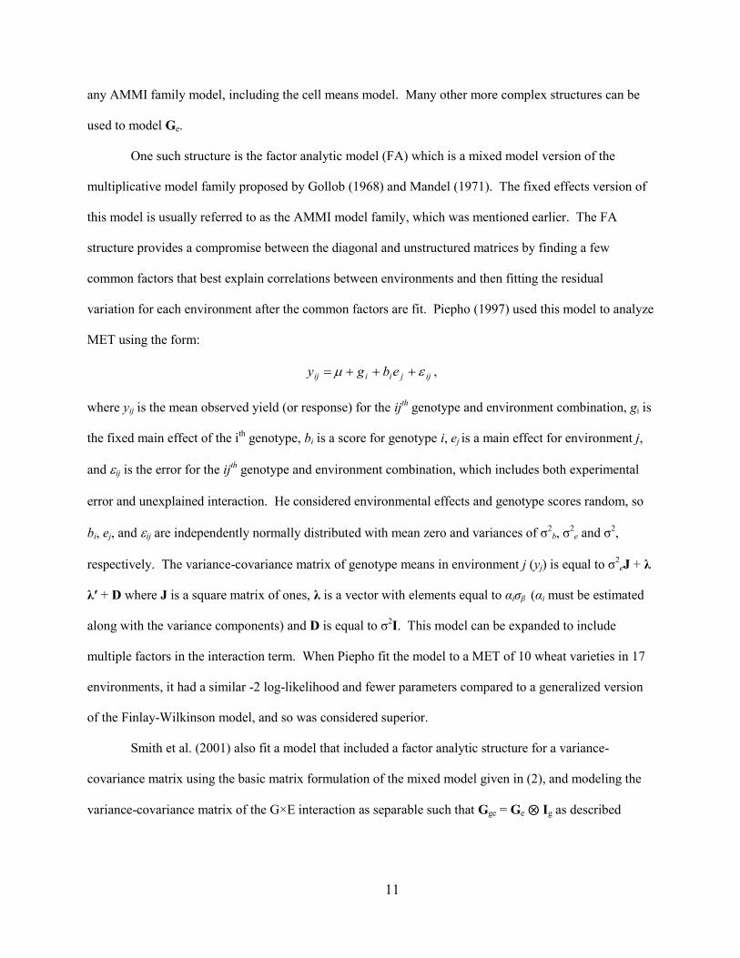
One such structure is the factor analytic model (FA) which is a mixed model version of the
multiplicative model family proposed by Gollob (1968) and Mandel (1971). The fixed effects version of
this model is usually referred to as the AMMI model family, which was mentioned earlier. The FA
structure provides a compromise between the diagonal and unstructured matrices by finding a few
common factors that best explain correlations between environments and then fitting the residual
variation for each environment after the common factors are fit. Piepho (1997) used this model to analyze
MET using the form:
ijjiiij ebgy ,
where yij is the mean observed yield (or response) for the ijth genotype and environment combination, gi is
the fixed main effect of the ith genotype, bi is a score for genotype i, ej is a main effect for environment j,
and ij is the error for the ijth genotype and environment combination, which includes both experimental
error and unexplained interaction. He considered environmental effects and genotype scores random, so
bi, ej, and ij are independently normally distributed with mean zero and variances of σ2
b, σ2
e and σ2,
respectively. The variance-covariance matrix of genotype means in environment j (yj) is equal to σ2
eJ + λ
λ′ + D where J is a square matrix of ones, λ is a vector with elements equal to αiσβ (αi must be estimated
along with the variance components) and D is equal to σ2I. This model can be expanded to include
multiple factors in the interaction term. When Piepho fit the model to a MET of 10 wheat varieties in 17
environments, it had a similar -2 log-likelihood and fewer parameters compared to a generalized version
of the Finlay-Wilkinson model, and so was considered superior.
Smith et al. (2001) also fit a model that included a factor analytic structure for a variance-
covariance matrix using the basic matrix formulation of the mixed model given in (2), and modeling the
variance-covariance matrix of the G×E interaction as separable such that Gge = Ge ⨂ Ig as described

12
above. A factor analytic model for Ge was modeled including the random effect of genotypes within
environments (γ) as:
δfu )( IΛg ,
where Λ is a matrix whose columns are known as loadings, f is a vector that can be partitioned into
factors corresponding to the columns of Λ, and δ is a vector of residuals (or specific variances). The
vectors f and δ have independent multivariate normal distributions with mean 0, and variance-covariances
of I and Ψ ⨂ I, respectively. The variance-covariance matrix for γ is:
IΨΛΛγ
IΛIΛγ
var
varvarvar δf
Smith et al. (2005) showed that the model used by Piepho (1997) can be specified in a matrix algebraic
form similar to that used by Smith et al. (2001). However, Smith et al. (2001) considered genotypes to be
random effects with fixed effects for environments, did not include a main effect for genotype in some
models, used heterogeneous specific variances (Ψ as opposed to Piepho‟s σ2I), and included a spatial
model for within-field variation. Both of these models assumed that genetic effects were independent.
Fitting this model to a MET with 172 genotypes in 7 locations, Smith et al. found that a two factor model
fit the data nearly as well as an unstructured Ge as judged by a likelihood ratio test.
As described above, researchers have attempted to improve the predictive accuracy of analyses of
MET by either incorporating pedigree data or FA structures into models of G×E variance. Crossa et al
(2006) and Oakey et al. (2007) went one step further and combined pedigree data with a FA structure for
environmental covariances. Crossa et al. modeled the variance covariance matrix of effects of genotypes
within environments as:
Aγ 1var g ,
where A is the additive relationship matrix, and Σg1 is a structure that models genetic variance and
covariance across environments. Crossa et al. used multiple structures ranging from independent and
identical variances to FA structures. Oakey et al. used a model similar to Smith et al. (2001), except for a
13
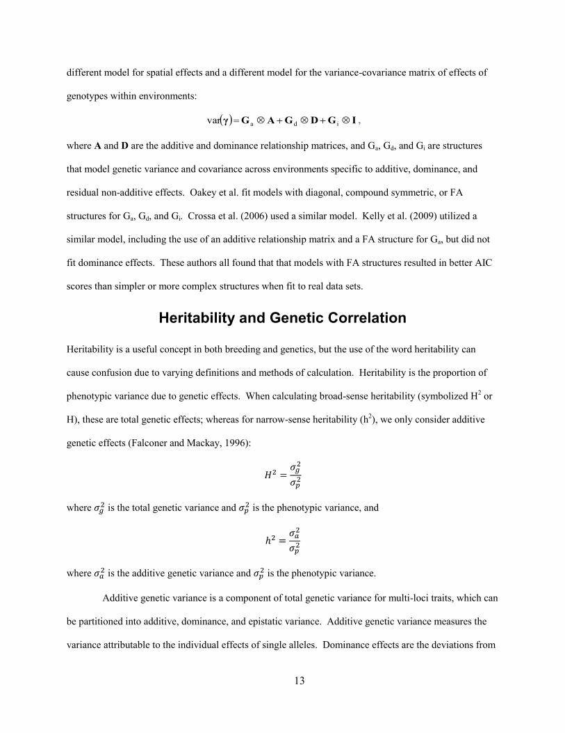
different model for spatial effects and a different model for the variance-covariance matrix of effects of
genotypes within environments:
IGDGAGγ idavar ,
where A and D are the additive and dominance relationship matrices, and Ga, Gd, and Gi are structures
that model genetic variance and covariance across environments specific to additive, dominance, and
residual non-additive effects. Oakey et al. fit models with diagonal, compound symmetric, or FA
structures for Ga, Gd, and Gi. Crossa et al. (2006) used a similar model. Kelly et al. (2009) utilized a
similar model, including the use of an additive relationship matrix and a FA structure for Ga, but did not
fit dominance effects. These authors all found that that models with FA structures resulted in better AIC
scores than simpler or more complex structures when fit to real data sets.
Heritability and Genetic Correlation
Heritability is a useful concept in both breeding and genetics, but the use of the word heritability can
cause confusion due to varying definitions and methods of calculation. Heritability is the proportion of
phenotypic variance due to genetic effects. When calculating broad-sense heritability (symbolized H2 or
H), these are total genetic effects; whereas for narrow-sense heritability (h2), we only consider additive
genetic effects (Falconer and Mackay, 1996):
where is the total genetic variance and
is the phenotypic variance, and
where is the additive genetic variance and
is the phenotypic variance.
Additive genetic variance is a component of total genetic variance for multi-loci traits, which can
be partitioned into additive, dominance, and epistatic variance. Additive genetic variance measures the
variance attributable to the individual effects of single alleles. Dominance effects are the deviations from

14
the additive effect of each allele that are observed to occur in heterozygous individuals, due to the
interactions between alleles at a locus. Epistasis refers to the interactions between genes or loci that
deviate from simple additive effects. Epistatic interactions can be among additive and/or dominance
effects and can be among two or more loci. Although the occurrence of epistatic effects is widely
acknowledged, estimation of epistatic effects is often limited by statistical power or experimental design.
Partly for this reason, epistasis is often assumed to be zero or negligible. When epistasis is estimated, the
number of interacting loci is often limited to two and dominance interactions may not be evaluated (Reif
et al., 2009; Duthie et al., 2010). If parents and offspring can be evaluated in the same environment,
covariance between parents and offspring and covariance between full-sib offspring can be used to
estimate additive, dominance, and additive*additive variance (Hallauer and Filho, 1981 pp. 49–52).
Diallel mating designs, with crosses between all pairs of n parents, can be used to estimate and
,
assuming no epistasis (Hallauer and Filho, 1981 pp. 52–60). Theoretically, crosses between three and
four parents can be used to isolate ,
, and , but their use is limited due to the complexity in
obtaining parents and crosses (Hallauer and Filho, 1981 pp. 83–88). Epistatic effects and the other
variance components can be easily estimated for populations in Hardy-Weinberg equilibrium with other
strict assumptions, but in reality, these assumptions are often violated. This makes estimation of variance
components more difficult and may necessitate other assumptions such as no epistasis (Lynch and Walsh,
1998 pp. 141–170).
Beyond broad and narrow-sense definitions, the definition of heritability must be further
specialized for specific uses. In animal breeding and evolutionary genetics, the individual is the unit of
interest; therefore, phenotypic and genetic variance among individuals is used in calculations (Visscher et
al., 2008). In plant breeding, many individuals with the same genotype can be produced, allowing for
replicated testing. Selection can then occur based on means of individuals with the same genotype. This
situation changes the definition of heritability so that the phenotypic variance is adjusted based on the unit
of selection and response (Holland et al., 2003). For example, if genotypes are selected based on means
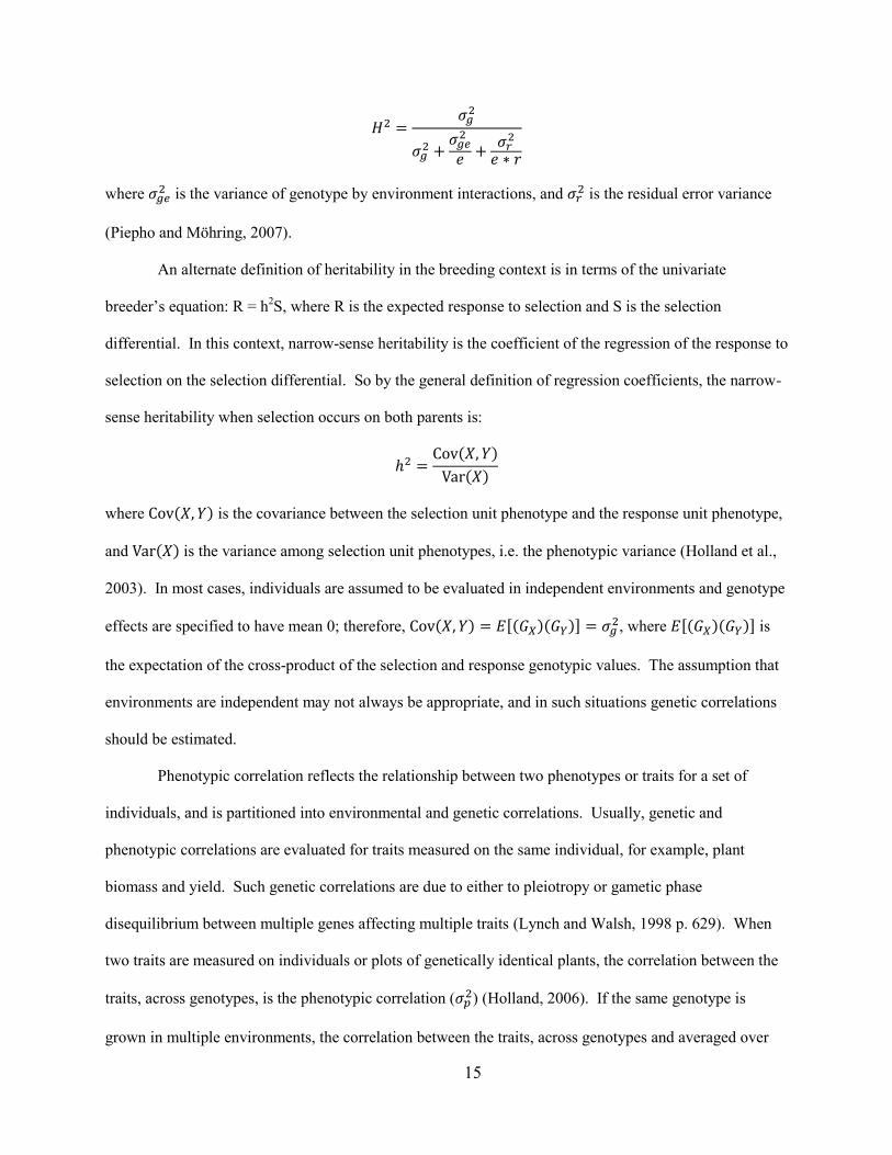
over e environments and r replicates within environments, broad sense heritability is:
15
where is the variance of genotype by environment interactions, and
is the residual error variance
(Piepho and Möhring, 2007).
An alternate definition of heritability in the breeding context is in terms of the univariate
breeder‟s equation: R = h2S, where R is the expected response to selection and S is the selection
differential. In this context, narrow-sense heritability is the coefficient of the regression of the response to
selection on the selection differential. So by the general definition of regression coefficients, the narrow-
sense heritability when selection occurs on both parents is:
where is the covariance between the selection unit phenotype and the response unit phenotype,
and is the variance among selection unit phenotypes, i.e. the phenotypic variance (Holland et al.,
2003). In most cases, individuals are assumed to be evaluated in independent environments and genotype
effects are specified to have mean 0; therefore, , where is
the expectation of the cross-product of the selection and response genotypic values. The assumption that
environments are independent may not always be appropriate, and in such situations genetic correlations
should be estimated.
Phenotypic correlation reflects the relationship between two phenotypes or traits for a set of
individuals, and is partitioned into environmental and genetic correlations. Usually, genetic and
phenotypic correlations are evaluated for traits measured on the same individual, for example, plant
biomass and yield. Such genetic correlations are due to either to pleiotropy or gametic phase
disequilibrium between multiple genes affecting multiple traits (Lynch and Walsh, 1998 p. 629). When
two traits are measured on individuals or plots of genetically identical plants, the correlation between the
traits, across genotypes, is the phenotypic correlation ( ) (Holland, 2006). If the same genotype is
grown in multiple environments, the correlation between the traits, across genotypes and averaged over

16
all environments, is the genetic correlation ( ). The difference between the two is the correlation
between the two traits when measured in the same environment (
), in this case the same
location, year and place in the field. Genotypes can be grown in multiple plots in the same field to parse
out the correlation due to position in the field (microenvironment) and year and location combination
(macroenvironment).
An alternative is to consider the responses of a genotype in different environments to be different
traits; the genetic correlation is then defined as the correlation between the responses of a set of genotypes
evaluated in two macroenvironments (Falconer, 1952). However, in this situation, the only
environmental and phenotypic correlations are on the scale of the microenvironments within the
macroevironments, and these correlations cannot be evaluated, since microenvironments cannot be
replicated. When treating responses to environments as traits, the genetic correlation is related to G×E,
where genetic correlations of less than one result from genotype by environment interactions (Lynch and
Walsh, 1998 pp. 660–665):
ignoring nonadditive genetic effects, where is the additive genetic correlation, is the variance of
genetic effects, and is the variance of interaction effects (differences in responses to the two
environments varying among genotypes). This relationship means that instead of the traditional fixed
effects ANOVA approach of modeling genotype by environment interactions as effects specific to each
genotype and environment combination, effects of genotypes within environments can be modeled as
correlated random effects that covary between environments and genotypes. This random effects
approach is described in detail in the Mixed Models for Multiple Environment Trials section.
Both heritability and genetic correlation are defined in terms of variance and covariance
parameters that are unknown in reality, and this necessitates estimation of these parameters, generally
through the use of mixed linear models with restricted maximum likelihood estimation. For heritability
estimations, the specific mixed model used depends on the relatedness among selection and response

17
individuals and on the structure of evaluation trials (Holland et al., 2003). This complexity and the
relationship above between the response to selection and realized heritability, led Piepho and Möhring
(2007) to propose a method to simulate values such as response to selection rather than heritability per se.
Estimation of genetic correlation is somewhat more straightforward, as it only depends upon relationship
and trial structures for the population evaluated (Holland, 2006).
Variance, heritability, and genetic correlation are often estimated in a single study and then
considered representative of a population, and this is valid, to the extent that the population represented
remains the one of interest. If any of these parameters are estimated in a study of one set of genetic
material, their application to another may be questionable, depending upon the differences between them.
Heritability and genetic variance will change over time due to selection, inbreeding, or mutation, which
change allelic frequencies and may change additive effects of alleles on a population basis (Visscher et
al., 2008). Heritability estimated for a set of breeding material may change in later years as new material
is introgressed and/or selection removes or reduces the frequency of inferior alleles. For example, if,
through selection, an allele becomes fixed, that locus will no longer contribute to additive effects for that
trait in that population. However, the effect may again become evident if a different allele is reintroduced
into the population. Genetic correlation between two environments may vary as weather conditions may
be more or less similar year-to-year.
Dimension Reduction for Linear Modeling
When fitting multiple linear models, one major assumption is that all explanatory variables are
independent of each other. A major consequence of violating this assumption is that the parameter
estimates for the multicollinear variables will have very large sampling variability and so do not provide
reliable information about the true parameter values (Kutner et al., 2004). The goal of many
observational studies is to evaluate multiple variables to determine which of them have the greatest effect
on a particular response. Statistical analysis of such studies will only be successful if the issue of
multicollinearity is resolved.

18
Multiple remedial measures are available for addressing multicollinearity, one of which is
dimension reduction. Dimension reduction techniques can be used to convert multicollinear variables
into a smaller number of independent variables, creating new variables that are functions of the original
multicollinear variables. Two dimension reduction techniques commonly used to eliminate
multicollinearity are principal components analysis and factor analysis.
Principal components analysis (PCA) is used for dimension reduction by replacing the original
variables with the first few principal components (Lattin et al., 2002). These principal components are
linear combinations of the original variables that are selected one at a time for maximum variance:
where
indicates the value of ui for which the bracketed quantity is maximized, zi is the vector of
scores for the ith scaled principal component, ui is the i
th eigenvector, X is the standardized original data,
R is the sample correlation matrix, and q is the number of original variables. This maximization problem
is solved using an eigenvalue or spectral decomposition of R. Additionally, PCA is equivalent to the
singular value decomposition of X. After PCA, the scores of the first few principal components can be
used to replace the observations of the original variables. Principal components are mutually
independent, and when calculated on a dataset with high multicollinearity, the first few can capture most
of the variation in the original variables. This makes PCA a useful option for dimension reduction prior
to linear regression.
Factor analysis and PCA are very similar but differ in terms of the specific model used for
dimension reduction. Like PCA, factor analysis can be used to generate a smaller set of new variables,
which capture most of the variation in the original variables by decomposing the correlation matrix of the
original variables (Lattin et al., 2002). Unlike PCA, in factor analysis variation not accounted for by the
factors is attributed to specific variance terms for each of the original variables. The new variables
identified in factor analysis are often referred to as latent factors, and are considered to be the true
unmeasurable factors, measured with error by the original variables, that affect the response (Suhr, 2005).

19
The number of new variables generated from either PCA or Factor analysis can range from 1 up
to the number of original variables and multiple techniques can be used to decide how many to keep
(Lattin et al., 2002). A scree plot of eigenvalues versus their associated component/factor can identify the
point at which the eigenvalues decrease in a linear fashion. Since the eigenvalues relate to the variance
explained by each component/factor, only retaining those that are above this linear trend results in a
parsimonious set that account for a large share of the original variation. Alternatively, Kaiser‟s Rule
suggests that only those variables with eigenvalues of greater than 1 should be retained, because each of
the standardized original variables has variance of 1 and thus the new variables should account for more
variation. Horn‟s procedure uses cutoffs like Kaiser‟s Rule, but with cutoffs of the eigenvalues from a
PCA of random data, generated with numbers of variables and observations equal to the original data.
Alternatively, a number of new variables can be retained such that they explain a user-defined proportion
of the variation in the original data or each specific original variable.
Following both PCA and factor analysis, rotation of the solution (a transformation of the matrix
of principal components/factors) may be used to aid in interpretation (Lattin et al., 2002). In the initial
results from PCA and principal factor analysis the first factor is chosen to maximize the variance
accounted for and is often partially correlated to many of the original variables. With rotation, new
factors can be generated that are highly related to some of the original variables and mostly unrelated to
the others. Rotation should be conducted after the final number of components or factors is chosen. The
methods of rotation can be divided into two major groups, those that result in orthogonal factors and those
that allow non-orthogonal factors. When the goal is to generate new variables to use in linear modeling,
orthogonality/independence is usually preferred. The advantage of non-orthogonal rotation is that it
allows for new variables that are related to more distinct subsets of the original variables. The easier
interpretation of non-orthogonal rotation can be advantageous in an observational study, but any resulting
lack of independence will make linear model coefficient estimates inaccurate.
20
Extreme Cold Tolerance in Wheat
Winter wheat is planted in autumn and requires a period of cold vernalization before flowering can occur.
However, not all winter wheat cultivars are able to survive the extreme cold that occurs in some
environments, resulting in winterkill that often causes economically important yield losses (Patterson et
al., 1990). Extreme cold can occur in winter wheat growing areas of Washington State and can result in
observed losses of 70% in an extreme year (Allen et al., 1992). Breeding winter wheat to tolerate extreme
cold is therefore an important goal for wheat breeders in Washington. Winter wheat genotypes vary in
their ability to survive extreme cold and this cold tolerance is controlled by genes on multiple
chromosomes (Sutka, 1994). Expression levels of a large number of genes change when wheat is exposed
to extreme cold and these changes vary across genotypes (Skinner, 2009). Additional work will be
necessary before breeders will be able to select for superior cold tolerance based on genetic information
alone.
Due to the complex genetic nature of wheat cold tolerance, differential phenotypic assessments
are necessary for the selection of breeding lines with greater cold tolerance. Assessment of cold tolerance
in the field is impaired by year to year variation in temperature conditions and variation in conditions
across a field, especially due to variable snow cover (Fowler, 1978). For this reason, evaluations under
controlled environments are more appropriate. Testing is generally conducted by subjecting vernalized
plants at an early growth stage to temperatures that decrease below freezing to a point where survival is
differential among genotypes, followed by slow warming to regular greenhouse temperatures. After a
number of weeks of regrowth plants are scored for survival. Beyond these generalities, numerous
variations have been implemented, including variations in temperature and time at each temperature
(Sutka, 1994; Fowler and Limin, 2004; Reddy et al., 2006; Skinner and Mackey, 2009; Skinner and
Bellinger, 2010).
When saturated soil is exposed to temperatures that decrease rapidly to a point well below
freezing, substantial differences in soil temperatures can occur (Skinner and Mackey, 2009). These

21
differences can be explained by variation in the amount of soil and water in each container that can occur
due to accidental differences in soil packing and heterogeneity in the soil or other planting media.
Containers with more soil and water will take longer to cool or warm, especially during the phase change
as water freezes. Holding the temperature just below freezing for an extended period of time allows the
water in all containers of soil to freeze, reducing variation in temperatures beyond that point. When
exposed to temperatures slightly below freezing (-3°C) for extended periods of time, wheat acquires
increased tolerance to extreme temperatures as compared to shorter periods just below freezing in a
process referred to as sub-zero acclimation (Herman et al., 2006). In the field, such a period of moderate
cold does not always precede an extreme cold event. Therefore, testing for cold tolerance including such
a sub-zero acclimation period may not precisely reflect tolerance in the field. However, the improved
consistency resulting from a sub-zero acclimation period may outweigh this concern. Even with a sub-
zero acclimation period, small differences in temperature may be present among samples, so it may be
beneficial to include temperature measurements in analyses.
The method for analyzing cold tolerance data depends upon the tolerance rating method and any
explanatory variables to be included. Cold tolerance is generally evaluated in terms of numbers of plants
surviving a cold event, but it can also be judged on an ordinal scale in terms of quality of regrowth (Sutka,
1994; Vagujfalvi et al., 2003). While both of these methods involve some subjective judgment, binary
survival is easier to judge and thus likely to be more consistent among researchers. Binary survival data
can be analyzed by treating each plant as an experimental unit or by using the proportion of plants that
survived as the response for each group of plants. If each plant is considered an experimental unit, the
data may be analyzed using logistic regression. Using the proportion approach, researchers have analyzed
survival data using analysis of variance on transformed proportions (Skinner and Mackey, 2009) and have
compared genotypes using the temperature at which 50% of the plants are killed (Limin and Fowler,
1993, 2006) or area under the death progress curve over a range of temperatures (Reddy et al., 2006).
If phenotypic evaluation of extreme cold tolerance is to be included in a breeding program,
evaluations must rapidly segregate large numbers of genotypes into groups with sufficient and insufficient

22
cold tolerance. Exact estimation of absolute tolerance levels is not necessary, but it is necessary to ensure
that placement of each genotype into each group is due to true genetic differences and not random chance.
Therefore, statistical testing that determines if each genotype has significantly different odds of survival
as compared to a control is an effective analysis method. Rapid evaluation of large numbers of genotypes
necessitates minimizing the number of times each genotype must be grown and placed in a freeze
chamber. Using a single cooling profile allows for more efficient testing as compared to testing each
genotype at multiple temperatures. However, it is important to identify beforehand a temperature profile
that is both differential among genotypes and provides cold tolerance assessments that accurately predict
performance in the field.
References
Agrama, H.A., W. Yan, F. Lee, R. Fjellstrom, M.-H. Chen, M. Jia, and A. McClung. 2009.
Genetic assessment of a mini-core subset developed from the USDA rice genebank. Crop
Science. 49(4): 1336–1346.
Allen, R.E., J.A. Pritchett, and L.M. Little. 1992. Cold injury observations. Anual Wheat
Newsletter. 38.
Anderson, W.F. 2005. Development of a forage bermudagrass (Cynodon sp.) core collection.
Grassland Science. 51: 305–308.
Balfourier, F., V. Roussel, P. Strelchenko, F. Exbrayat-Vinson, P. Sourdille, G. Boutet, J.
Koenig, C. Ravel, O. Mitrofanova, M. Beckert, and G. Charmet. 2007. A worldwide
bread wheat core collection arrayed in a 384-well plate. Theoretical and Applied
Genetics. 114: 1265–1275.
Basigalup, D.H., D.K. Barnes, and R.E. Stucker. 1995. Development of a core collection for
perennial Medicago plant introductions. Crop Science. 35: 1163–1168.
Bernardo, R. 1994. Prediction of maize single-cross performance using RFLPs and information
from related hybrids. Crop Science. 34(1): 20–25.
Bernardo, R. 1995. Genetic models for predicting maize single-cross performance in unbalanced
yield trial data. Crop Science. 35(1): 141–147.
Bernardo, R. 1996. Best linear unbiased prediction of maize single-cross performance. Crop
Science. 36(1): 50–56.

23
Bhattacharjee, R., I.S. Khairwal, P.J. Bramel, and K.N. Reddy. 2007. Establishment of a pearl
millet [Pennisetum glaucum (L.) R. Br.] core collection based on geographical
distribution and quantitative traits. Euphytica. 155: 35–45.
Brown, A.H.D. 1989. Core collections: a practical approach to genetic resources management.
Genome. 31: 818–824.
Cornelius, P.L., and J. Crossa. 1999. Prediction assessment of shrinkage estimators of
multiplicative models for multi-environment cultivar trials. Crop Science. 39(4): 998–
1009.
Crossa, J., J. Burgueño, P.L. Cornelius, G. McLaren, R. Trethowan, and A. Krishnamachari.
2006. Modeling genotype × environment interaction using additive genetic covariances
of relatives for predicting breeding values of wheat genotypes. Crop Science. 46(4):
1722–1733.
Dahlberg, J.A., J.J. Burke, and D.T. Rosenow. 2004. Development of a sorghum core collection:
refinement and evaluation of a subset from Sudan. Economic Botany. 58(4): 556–567.
Diwan, N., G.R. Bauchan, and M.S. McIntosh. 1995. Methods of developing a core collection of
annual Medicago species. Theoretical and Applied Genetics. 90: 755–761.
Duthie, C., G. Simm, A. Doeschl-Wilson, E. Kalm, P.W. Knap, and R. Roehe. 2010. Epistatic
analysis of carcass characteristics in pigs reveals genomic interactions between
quantitative trait loci attributable to additive and dominance genetic effects. Journal of
Animal Science. 88(7): 2219 –2234Available at (verified 20 January 2012).
Dwivedi, S.L., N. Puppala, H.D. Upadhyaya, N. Manivannan, and S. Singh. 2008. Developing a
core collection of peanut specific to Valencia market type. Crop Science. 48: 625–632.
Escribano, P., M.A. Viruel, and J.I. Hormaza. 2008. Comparison of different methods to
construct a core germplasm collection in woody perennial species with simple sequence
repeat markers. A case study in cherimoya (Annona cherimola, Annonaceae), an
underutilised subtropical fruit tree species. Annals of Applied Biology. 153: 25–32.
Falconer, D.S. 1952. The Problem of Environment and Selection. The American Naturalist.
86(830): 293–298.
Falconer, D.S., and T.F.C. Mackay. 1996. Introduction to Quantitative Genetics. 4th ed.
Benjamin Cummings.
Finlay, K., and G. Wilkinson. 1963. The analysis of adaptation in a plant-breeding programme.
Aust. J. Agric. Res. 14(6): 742–754.
Fowler, D.B. 1978. Selection for winterhardiness in wheat. II. variation within field trials. Crop
Science. 19(6): 773–775.

24
Fowler, D.B., and A.E. Limin. 2004. Interactions among factors regulating phenological
development and acclimation rate determine low-temperature tolerance in wheat. Annals
of Botany. 94(5): 717 –724.
Franco, J., J. Crossa, and S. Desphande. 2010. Hierarchical multiple-factor analysis for
classifying genotypes based on phenotypic and genetic data. Crop Sci. 50(1): 105–117.
Franco, J., J. Crossa, S. Taba, and H. Shands. 2005. A sampling strategy for conserving genetic
diversity when forming core subsets. Crop Science. 45: 1035–1044.
Franco, J., J. Crossa, J. Villasenor, A. Castillo, S. Taba, and S.A. Eberhart. 1999. A two-stage,
three-way method for classifying genetic resources in multiple environments. Crop
Science. 39: 259–267.
Franco, J., J. Crossa, J. Villasenor, S. Taba, and S.A. Eberhart. 1997. Classifying Mexican maize
accessions using hierarchical and density search methods. Crop Science. 37: 972–980.
Franco, J., J. Crossa, J. Villasenor, S. Taba, and S.A. Eberhart. 1998. Classifying genetic
resources by categorical and continuous variables. Crop Science. 38: 1688–1696.
Franco, J., J. Crossa, M.L. Warburton, and S. Taba. 2006. Sampling strategies for conserving
maize diversity when forming core subsets using genetic markers. Crop Science. 46:
854–864.
Gauch, H.G. 1988. Model selection and validation for yield trials with interaction. Biometrics.
44(3): 705–715.
Gauch, H.G., and R.W. Zobel. 1988. Predictive and postdictive success of statistical analyses of
yield trials. Theoret. Appl. Genetics. 76(1): 1–10.
Gollob, H.F. 1968. A statistical model which combines features of factor analytic and analysis of
variance techniques. Psychometrika. 33(1): 73–115.
Gower, J.C. 1971. A general coefficient of similarity and some of its properties. Biometrics. 27:
857–74.
Grenier, C., P.J. Bramel-Cox, and P. Hamon. 2001a. Core collection of sorghum: I. stratification
based on eco-geographical data. Crop Science. 41: 234–240.
Grenier, C., P. Hamon, and P.J. Bramel-Cox. 2001b. Core collection of sorghum: II. comparison
of three random sampling strategies. Crop Science. 41: 241–246.
Hallauer, A., and J.B.M. Filho. 1981. Quantitative Genetics in Maize Breeding. Iowa State
University Press, Ames.
Hao, C., Y. Dong, L. Wang, G. You, H. Zhang, H. Ge, J. Jia, and X. Zhang. 2008. Genetic
diversity and construction of core collection in Chinese wheat genetic resources. Chinese
Science Bulletin. 53(10): 1518–1526.

25
Hayes, B.J., P.M. Visscher, and M.E. Goddard. 2009. Increased accuracy of artificial selection
by using the realized relationship matrix. Genetics Research. 91(01): 47.
Henderson, C.R. 1973. Sire evaluation and genetic trends. J. Anim Sci. 1973(Symposium): 10–
41.
Henderson, C.R. 1976. A simple method for computing the inverse of a numerator relationship
matrix used in prediction of breeding values. Biometrics. 32(1): 69–83.
Herman, E.M., K. Rotter, R. Premakumar, G. Elwinger, R. Bae, L. Ehler-King, S. Chen, and
D.P. Livingston III. 2006. Additional freeze hardiness in wheat acquired by exposure to -
3C is associated with extensive physiological, morphological, and molecular changes.
Journal of Experimental Botany. 57(14): 3601–3618.
Hill, R.R., and J.L. Rosenberger. 1985. Methods for combining data from germplasm evaluation
trials. Crop Science. 25(3): 467–470.
Holbrook, C.C., and W. Dong. 2005. Development and evaluation of a mini core collection for
the U.S. peanut germplasm collection. Crop Science. 45: 1540–1544.
Holland, J.B. 2006. Estimating Genotypic Correlations and Their Standard Errors Using
Multivariate Restricted Maximum Likelihood Estimation with SAS Proc MIXED. Crop
Science. 46(2): 642–654.
Holland, J.B., W.E. Nyquist, and C.T. Cervantes-Martínez. 2003. Estimating and Interpreting
Heritability for Plant Breeding: An Update. : 9–112.
Hu, J., J. Zhu, and H.M. Xu. 2000. Methods of constructing core collections by stepwise
clustering with three sampling strategies based on the genotypic values of crops.
Theoretical and Applied Genetics. 101: 264–268.
Huamán, Z., R. Ortiz, and R. Gómez. 2000. Selecting a Solanum tuberosum subsp. andigena
core collection using morphological, geographical, disease and pest descriptors.
American Journal of Potato Research. 77: 183–190.
Igartua, E., M.P. Gracia, J.M. Lasa, B. Medina, J.L. Molina-Cano, J.L. Montoya, and I.
Romagosa. 1998. The Spanish barley core collection. Genetic Resources and Crop
Evolution. 45: 475–481.
Kang, C.W., S.Y. Kim, S.W. Lee, P.N. Mathur, T. Hodgkin, M.D. Zhou, and J.R. Lee. 2006.
Selection of a core collection of Korean sesame germplasm by a stepwise clustering
method. Breeding Science. 56: 85–91.
Kelly, A., B.R. Cullis, A.R. Gilmour, J.A. Eccleston, and R. Thompson. 2009. Estimation in a
multiplicative mixed model involving a genetic relationship matrix. Genetics Selection
Evolution. 41: 33–42.

26
Kroonenberg, P.M., B.D. Harch, K.E. Basford, and A. Cruickshan. 1997. Combined analysis of
categorical and numerical descriptors of australian groundnut accessions using nonlinear
principal component analysis. Journal of Agricultural, Biological, and Environmental
Statistics. 2(3): 294–312.
Kutner, M., C. Nachtsheim, J. Neter, and W. Li. 2004. Applied Linear Statistical Models. 5th ed.
McGraw-Hill/Irwin, San Francisco.
Lattin, J., D. Carroll, and P. Green. 2002. Analyzing Multivariate Data. 1st ed. Duxbury Press.
Li, C.T., C.H. Shi, J.G. Wu, H.M. Xu, H.Z. Zhang, and Y.L. Ren. 2004. Methods of developing
core collections based on the predicted genotypic value of rice (Oryza sativa L.).
Theoretical and Applied Genetics. 108: 1172–1176.
Limin, A.E., and D.B. Fowler. 1993. Inheritance of cold hardiness in Triticum aestivum ×
synthetic hexaploid wheat crosses. Plant Breeding. 110(2): 103–108.
Limin, A.E., and D.B. Fowler. 2006. Low-temperature tolerance and genetic potential in wheat
(Triticum aestivum L.): response to photoperiod, vernalization, and plant development.
Planta. 224(2): 360–366.
Lynch, M., and B. Walsh. 1998. Genetics and Analysis of Quantitative Traits. 1st ed. Sinauer
Associates.
Mahalakshmi, V., Q. Ng, M. Lawson, and R. Ortiz. 2006. Cowpea [Vigna unguiculata (L.)
Walp.] core collection defined by geographical, agronomical and botanical descriptors.
Plant Genetic Resources: Characterization and Utilization. 5(3): 113–119.
Mandel, J. 1971. A new analysis of variance model for non-additive data. Technometrics. 13(1):
1–18.
Miklas, P.N., R. Delorme, R. Hannan, and M.H. Dickson. 1999. Using a subsample of the core
collection to identify new sources of resistance to white mold in common bean. Crop
Science. 39: 569–573.
Mrode, R.A., and R. Thompson. 2005. Linear models for the prediction of animal breeding
values. 2nd ed. CABI, Cambridge, MA.
Oakey, H., A.P. Verbyla, B.R. Cullis, X. Wei, and W.S. Pitchford. 2007. Joint modeling of
additive and non-additive (genetic line) effects in multi-environment trials. Theoretical
and Applied Genetics. 114: 1319–1332.
Panter, D.M., and F.L. Allen. 1995a. Using best linear unbiased predictions to enhance breeding
for yield in soybean: I. choosing parents. Crop Science. 35(2): 397–405.
Panter, D.M., and F.L. Allen. 1995b. Using best linear unbiased predictions to enhance breeding
for yield in soybean: II. selection of superior crosses from a limited number of yield
trials. Crop Science. 35(2): 405–410.

27
Parra-Quijano, M., J.M. Iriondo, E. Torres, and L.D. la Rosa. 2011. Evaluation and Validation of
Ecogeographical Core Collections using Phenotypic Data. Crop Science. 51(2): 694.
Pattee, H.E., T.G. Isleib, D.W. Gorbet, F.G. Giesbrecht, and Z. Cui. 2001. Parent selection in
breeding for roasted peanut flavor quality. Peanut Science. 28(2): 51–58.
Patterson, F.L., G.E. Shaner, H.W. Ohm, and J.E. Foster. 1990. A historical perspective for the
establishment of research goals for wheat improvement. Journal of Production
Agriculture. 3(1): 30–38.
Piepho, H.-P. 1994. Best Linear Unbiased Prediction (BLUP) for regional yield trials: a
comparison to additive main effects and multiplicative interaction (AMMI) analysis.
Theoret. Appl. Genetics. 89(5).
Piepho, H.-P. 1997. Analyzing genotype-environment data by mixed models with multiplicative
terms. Biometrics. 53(2): 761–766.
Piepho, H.-P., and J. Möhring. 2007. Computing Heritability and Selection Response From
Unbalanced Plant Breeding Trials. Genetics. 177(3): 1881 –1888.
Piepho, H.-P., J. Mohring, A.E. Melchinger, and A. Buchse. 2008. BLUP for phenotypic
selection in plant breeding and variety testing. Euphytica. 161: 209–228.
Rao, K.E.P., and V.R. Rao. 1995. The use of characterisation data in developing a core collection
of sorghum. p. 109–115. In Core Collections of Plant Genetic Resources. John Wiley &
Sons, Chichester.
Reddy, L., R.E. Allan, and K.A. Garland Campbell. 2006. Evaluation of cold hardiness in two
sets of near-isogenic lines of wheat (Triticum aestivum) with polymorphic vernalization
alleles. Plant Breeding. 125(5): 448–456.
Reddy, L.J., H.D. Upadhyaya, C.L.L. Gowda, and S. Singh. 2005. Development of core
collection in pigeonpea [Cajanus cajan (L.) Millspaugh] using geographic and qualitative
morphological descriptors. Genetic resources and crop evolution. 52: 1049–1056.
Reif, J.C., B. Kusterer, H.-P. Piepho, R.C. Meyer, T. Altmann, C.C. Schön, and A.E.
Melchinger. 2009. Unraveling Epistasis With Triple Testcross Progenies of Near-
Isogenic Lines. Genetics. 181(1): 247 –257Available at (verified 20 January 2012).
Rodiño, A.P., M. Santalla, A.M. De Ron, and S.P. Singh. 2003. A core collection of common
bean from the Iberian peninsula. Euphytica. 131: 165–175.
Skinner, D.Z. 2009. Post-acclimation transcriptome adjustment is a major factor in freezing
tolerance of winter wheat. Functional & Integrative Genomics. 9(4): 513–523.
Skinner, D.Z., G.R. Bauchan, G. Auricht, and S. Hughes. 1999. A method for the efficient
management and utilization of large germplasm collections. Crop Science. 39: 1237–
1242.

28
Skinner, D.Z., and B.S. Bellinger. 2010. Exposure to subfreezing temperature and a freeze-thaw
cycle affect freezing tolerance of winter wheat in saturated soil. Plant and Soil. 332: 289–
297.
Skinner, D.Z., and B. Mackey. 2009. Freezing tolerance of winter wheat plants frozen in
saturated soil. Field Crops Research. 113(3): 335–341.
Smith, A., B. Cullis, and R. Thompson. 2001. Analyzing variety by environment data using
multiplicative mixed models and adjustments for spatial field trend. Biometrics. 57(4):
1138–1147.
Smith, A.B., B.R. Cullis, and R. Thompson. 2005. The analysis of crop cultivar breeding and
evaluation trials: an overview of current mixed model approaches. The Journal of
Agricultural Science. 143(06): 449–462.
Suhr, D. 2005. Principal Component Analysis vs. Exploratory Factor Analysis. In Proceedings of
the Thirtieth Annual SAS Users Group International Conference. SAS Institute Inc.,
Cary, NC.
Sutka, J. 1994. Genetic control of frost tolerance in wheat (Triticum aestivum L.). Euphytica. 77:
277–282.
Tai, P.Y.P., and J.D. Miller. 2001. A core collection for Saccharum spontaneum L. from the
world collection of sugarcane. Crop Science. 41: 879–885.
Upadhyaya, H.D., P.J. Bramel, and S. Singh. 2001. Development of a chickpea core subset using
geographic distribution and quantitative traits. Crop Science. 41: 206–210.
Upadhyaya, H.D., C.L.L. Gowda, R.P.S. Pundir, V.G. Reddy, and S. Singh. 2006. Development
of core subset of finger millet germplasm using geographical origin and data on 14
quantitative traits. Genetic resources and crop evolution. 53: 679–685.
Upadhyaya, H.D., R.P.S. Pundir, C.L.L. Gowda, V.G. Reddy, and S. Singh. 2008. Establishing a
core collection of foxtail millet to enhance the utilization of germplasm of an
underutilized crop. Plant Genetic Resources: Characterization and Utilization. 6: 1–8.
USDA ARS, National Genetic Resources Program. 2009. Germplasm Resources Information
Network - (GRIN). [Online Database] National Germplasm Resources Laboratory,
Beltsville, Maryland.Available at http://www.ars-grin.gov/cgi-
bin/npgs/html/desc.pl?65059 (verified 17 December 2009).
Vagujfalvi, A., G. Galiba, L. Cattivelli, and J. Dubcovsky. 2003. The cold-regulated
transcriptional activator Cbf3 is linked to the frost-tolerance locus Fr-A2 on wheat
chromosome 5A. Molecular Genetics and Genomics. 269(1): 60–67.
Villanueva, B., R. Pong-Wong, J. Fernández, and M.A. Toro. 2005. Benefits from Marker-
Assisted Selection Under an Additive Polygenic Genetic Model. J ANIM SCI. 83(8):
1747–1752.

29
Visscher, P.M., W.G. Hill, and N.R. Wray. 2008. Heritability in the genomics era - concepts and
misconceptions. Nat Rev Genet. 9(4): 255–266.
Wang, X., R. Fjellstrom, Y. Jia, W.G. Yan, M.H. Jia, B.E. Scheffler, D. Wu, Q. Shu, and A.
McClung. 2010. Characterization of Pi-ta blast resistance gene in an international rice
core collection. Plant Breeding. 129(5): 491–501.
Wang, L., Y. Guan, R. Guan, Y. Li, Y. Ma, Z. Dong, X. Liu, H. Zhang, Y. Zhang, Z. Liu, R.
Chang, H. Xu, L. Li, F. Lin, W. Luan, Z. Yan, X. Ning, L. Zhu, Y. Cui, R. Piao, Y. Liu,
P. Chen, and L. Qiu. 2006. Establishment of Chinese soybean (Glycine max) core
collections with agronomic traits and SSR markers. Euphytica. 151: 215–223.
Weihai, M., Y. Jinxin, and D. Sihachakr. 2008. Development of core subset for the collection of
Chinese cultivated eggplants using morphological-based passport data. Plant Genetic
Resources: Characterization and Utilization. 6(1): 33–40.
Yan, W., N. Rutger, R.J. Bryant, H.E. Bockelman, R.G. Fjellstrom, M.-H. Chen, T.H. Tai, and
A.M. McClung. 2007. Development and evaluation of a core subset of the USDA rice
germplasm collection. Crop Science. 47: 869–878.
Yates, F., and W.G. Cochran. 1938. The analysis of groups of experiments. The Journal of
Agricultural Science. 28(04): 556–580.
30
CHAPTER 2
METHODS FOR SELECTING GERMPLASM CORE SUBSETS
USING SPARSE PHENOTYPIC DATA
Carl A. Walker, Harold E. Bockelman, J. Richard Alldredge, Kimberly Garland Campbell*
C.A. Walker, Dep. of Crop and Soil Sciences, Washington State Univ., Pullman, WA, 99164-
6420; K.G. Campbell, USDA-ARS, Wheat Genetics, Wheat Genetics, Quality, Physiology, and
Disease Research Unit, 209 Johnson Hall, Pullman, WA 99164-6420; H.E. Bockelman, USDA-
ARS, National Small Grains Collection, 1691 S 2700 W, Aberdeen, ID 83210; J.R. Alldredge,
Department of Statistics, Washington State University, Pullman, WA, 99164-6420
*Corresponding author ([email protected]).
Abbreviations: GRIN, Germplasm Research Information Network; HTAP, High-temperature
Adult Plant; RI, recovery of interquartile range; RM, recovery of median; RR recovery of range;
RS, recovery of Shannon index; UPGMA, unweighted pair-group method using arithmetic
averages.
Abstract
Crop plant germplasm collections are often too large and too lacking in descriptive data to be of
use regularly. A well-characterized core subset that consists of a reduced number of accessions
(usually about 10% of the total) can provide increased utility while still maintaining most of the
genetic diversity of the complete collection. Most core subsets have been constructed using
complete or nearly complete data sets of geographical, phenotypic, or genotypic data, but most
large germplasm collections only have complete, or even mostly complete, data for a few
31
variables. The main objective of this study was to evaluate methods for selecting core subsets of
germplasm collections using sparse geographic and phenotypic data. A subset of variables and
accessions with complete data was isolated from the USDA Triticum aestivum collection and
was used to simulate multiple collections with sparse data. Core subsets were selected from the
simulated data sets using 12 methods, defined by the choice of variables to use in Gower‟s
distance estimations, clustering algorithm, and sampling intensity. Diversity metrics were
calculated for each method and simulation. The methods were ranked within each simulation
and then compared in terms of these average rankings. We conclude that core subsets can be
selected based on sparse phenotypic data, and we recommend that a) Gower‟s distances should
be estimated using all variables available, including those with more than 5% missing data; b)
clustering should be conducted using the UPGMA algorithm; and c) clusters should be sampled
in proportion to the logarithm of the cluster sizes.

32
Introduction
Crop plant germplasm collections are maintained to conserve genetic variation and to provide
useful plant material for researchers and plant breeders. An example of such a collection, which
will be used in this study, is the collection of wheat (Triticum aestivum L. subsp. aestivum)
accessions maintained as part of the National Small Grains Collection of the USDA-ARS
National Plant Germplasm System (http://www.ars-grin.gov/npgs/index.html).
For many researchers and plant breeders, germplasm collections are often too large and
too lacking in descriptive data to be of regular use. A well-characterized core collection, or core
subset, that consists of a reduced number of accessions (usually about 10% of the total) can
provide increased utility while still maintaining most of the genetic diversity of the complete
collection (Brown, 1989). Therefore, the best method for selecting core subsets is the one that
results in the most diversity for a given number of accessions. Since desired alleles are unevenly
distributed throughout germplasm collections, preferentially selecting a portion from each
heterogeneous group present in a complete collection increases the likelihood of selecting these
unevenly distributed alleles (Brown, 1989). For this reason, most researchers have constructed
core collections by grouping accessions and then selecting accessions within groups.
A number of different methods and types of data have been used to group accessions and
select core collections. Passport data, i.e. the location of cultivation or collection, has been used
to stratify complete collections followed by selection from within each stratum. This technique
was used to select a core subset for the complete wheat collection described above (USDA ARS,
National Genetic Resources Program, 2009), and to develop other core collections (Skinner et
al., 1999; Huamán et al., 2000; Dahlberg et al., 2004; Yan et al., 2007). Other methods for
selecting core subsets have included stratification based on geographic origin, followed by

33
further grouping based on cluster analysis of phenotypic traits (Basigalup et al., 1995; Rao and
Rao, 1995; Igartua et al., 1998; Tai and Miller, 2001; Upadhyaya et al., 2001, 2006;
Mahalakshmi et al., 2006; Bhattacharjee et al., 2007; Dwivedi et al., 2008). Stratification of
collections has also been conducted using cluster analysis without prior geographic grouping
(Diwan et al., 1995; Franco et al., 1997, 1998, 1999, 2005; Grenier et al., 2001a; Li et al., 2004;
Anderson, 2005; Holbrook and Dong, 2005; Weihai et al., 2008; Upadhyaya et al., 2008). A
comparison of core subset selection methods using relatively complete phenotypic data,
demonstrated that selection based on clustering using those data was superior to selection based
on geographic origin alone (Diwan et al., 1995).
The clustering method and the data used in the clustering process have also varied,
resulting in dramatic differences in final grouping. Clustering methods used include Ward‟s
minimum variance (Franco et al., 1997; Hu et al., 2000; Upadhyaya et al., 2006, 2008, 2001;
Anderson, 2005; Holbrook and Dong, 2005; Reddy et al., 2005; Kang et al., 2006; Mahalakshmi
et al., 2006; Bhattacharjee et al., 2007; Dwivedi et al., 2008), unweighted pair-group method
using arithmetic average (UPGMA), also known as the average linkage method (Hu et al., 2000;
Huamán et al., 2000; Li et al., 2004; Franco et al., 2006; Weihai et al., 2008), complete linkage
(Hu et al., 2000), and the Ward-Modified Location method (Franco et al., 1998, 1999, 2005).
Core collections have been constructed using cluster analysis based on phenotypic
variables followed by random sampling. In many cases these variables have been uniformly
quantitative, and either Euclidian distances or principle components were used to determine
relationships among accessions and construct clusters (Diwan et al., 1995; Igartua et al., 1998;
Holbrook and Dong, 2005; Kang et al., 2006; Bhattacharjee et al., 2007; Upadhyaya et al., 2008).

34
Both categorical and quantitative variables have been used to determine clusters in a few cases
(Franco et al., 1997, 1998, 1999, 2005; Kroonenberg et al., 1997).
More recently, relationships have been determined based on genotypic data (Franco et al.,
2006; Wang et al., 2006; Balfourier et al., 2007; Escribano et al., 2008; Hao et al., 2008) or
combinations of genotypic and phenotypic data (Franco et al., 2010). Clusters constructed using
genotypic data likely result in core subsets that better capture the genetic diversity in the
complete collection; however, the germplasm collections for most major crop plants are too large
to genotype all accessions.
Following the stratification of the complete collection, by cluster analysis, a set of
accessions was chosen from each group with the number sampled based on the size or the
diversity of each group. Direct, or only partially random, selection of all or a portion of the
accessions in a core has been used to increase diversity (Basigalup et al., 1995; Skinner et al.,
1999; Huamán et al., 2000; Rodiño et al., 2003; Yan et al., 2007; Weihai et al., 2008). However,
most researchers have selected accessions from each group randomly and with equal chance of
selection among accessions in a group. Proportional sampling, where the number of accessions
was chosen according to the group size, has often been used to select core subsets (Basigalup et
al., 1995; Upadhyaya et al., 2001, 2006, 2008; Grenier et al., 2001b; Dahlberg et al., 2004;
Holbrook and Dong, 2005; Reddy et al., 2005; Bhattacharjee et al., 2007; Dwivedi et al., 2008).
Other sampling methods, such as selection in proportion to the square root of group size (square
root sampling) (Huamán et al., 2000; Wang et al., 2006) and selection based on the natural
logarithm of group size (logarthmic sampling) (Grenier et al., 2001b; Yan et al., 2007), took
relatively fewer samples from larger groups. These proportional sampling methods reduced
redundancy and increased variability, as larger clusters tend to have greater redundancy among

35
accessions (Brown, 1989). Diversity was also increased by directly selecting more accessions
from groups with greater relative diversity. For example, sampling numbers were determined
relative to the mean distance among accessions in each cluster (Franco et al., 2005).
One aspect of most core subsets, including those referenced above, is that they were
constructed using complete or nearly complete data sets of geographical, phenotypic, or
genotypic data. One exception was an approach by Basigalup et al. (1995), who used partial data
to manually select accessions with extreme values. Such a manual approach is time consuming
and necessarily requires subjective judgments or core subsets that increase in size with the
number of variables assessed. Most large germplasm collections have complete, or even mostly
complete, data for only a few geographic and phenotypic variables. The USDA soybean
collection is comprised of more than 17 thousand accessions, and 106 descriptors, but 75 of
those descriptors have data for less than 10 thousand accessions (Randall Nelson, personal
communication). The USDA wheat collection is even larger and more sparse (details below).
Therefore, methods that have previously been shown to produce diverse core subsets may not be
applicable or the most effective use of sparse data describing the largest germplasm collections
of major crop plants. While one option is to construct the core subset using only the complete, or
nearly complete, geographic and phenotypic data; the sparse data may well delineate differences
among heterogeneous accessions that would otherwise be grouped together.
How then should sparse data, such as the wheat GRIN database, be used to select core
subsets? Gower‟s distance (Gower, 1971) has been used to calculate distances between
accessions based on variables, of any measurement level (nominal, ordinal, interval, or ratio), for
which both accessions have values. When either accession has a missing value for a variable,
that variable would not be included in the calculation. Thus, sparse data can be used to calculate

36
distances, but it may not be appropriate to do so. If data are not missing at random, then
parameter estimates calculated from such data will be biased (Graham, 2009). That is, estimates
of distances between accessions may be influenced by which variables have missing values.
In some cases, however, biased estimates using all data available may be preferable to
unbiased estimates using a very small proportion of the total data available, because they result
in reduced variance among distance calculations. Intuitively, if two accessions are known to be
different for a trait, that information should be included, rather than ignored, when making
decisions about relatedness. Decisions about whether or not to use sparse data in distance
calculations should be based on the diversity of the resulting core subsets.
The main objective of this study was to evaluate methods for selecting core subsets of
germplasm collections using sparse geographic and phenotypic data. We compared methods by
repeatedly selecting core subsets from a complete collection with data sets simulated to have
differing patterns of missing values. We then evaluated the core subsets, selected using each
method, in terms of their capture of the diversity present in the complete collection. A second
objective was to recommend a strategy for using all data available to construct core germplasm
collections.
Materials and Methods
The Germplasm Research Information Network (GRIN) maintains a database of all species held
by the National Genetic Resources Program, including wheat accessions held by the USDA-ARS
National Small Grains Collection. The wheat information in the database includes species,
identification information (accession number, name and improvement status), passport data
(country and state where the accession was collected), growth habit, and 77 other variables
reflecting agronomic, descriptive, disease susceptibility, and insect susceptibility data. However,

37
as is the case for many species curated in the National Genetic Resources Program, this data set
is far from complete, as many agronomic and susceptibility tests have been only been conducted
on a portion of the accessions. For accessions of Triticum aestivum subsp. aestivum, the
variables range from greater than 99.9% complete for country of origin, to more than 99%
missing values (Table 1). Ongoing evaluations are being conducted for several traits. At the
time this project was initiated, 41,312 accessions of Triticum aestivum subsp. aestivum were
included in the database.
A total of 3160 accessions from the USDA wheat collection have complete data for 23
variables (Table 2, first column). This subset of variables and accessions will be referred to as
the “complete” collection and was used to simulate multiple collections with sparse data. To
reduce the possibility that our conclusions would rely on a particular set or pattern of missing
data, four patterns of missing data were evaluated. Independently for each variable, values were
removed by randomly choosing accessions from a uniform distribution, i.e. missing completely
at random (MCAR), or, for each variable, values were removed from a randomly chosen
contiguous set of accessions (MC). For each of these two methods of removal, two sets of
percentages of missing values were assigned to the 23 variables (Table 2). The first set of values
was chosen to resemble the general pattern of missing value amounts observed among the
variables in the complete collection (Table 1), with the same variables best represented. The
second pattern was the reverse of the first and of the data structure of the complete collection.
No values were removed from country of origin, since this information is available for almost all
accessions. For each of these four patterns of missing data (MCAR-1, MC-1, MCAR-2, and
MC-2), 200 independent data sets were simulated by removing values from the “complete”
collection (referred to as the simulations).

38
There are important functional differences between MCAR and MC patterns, because
accessions in the USDA complete collection and the “complete” collection are ordered based on
when they were added to the collection and frequently characterized in that order. Since
accessions were added to the collection in groups that often had a degree of genetic similarity
(e.g. cultivars from a single breeding program), missing values from a contiguous set could
influence the best choice of method for selecting a core subset using sparse phenotypic data.
In order to evaluate the utility of selecting core subsets using the sparse passport and
phenotypic data from the GRIN database, multiple core selection methods were applied to the
simulated data sets and compared. All methods began with the calculation of a matrix of
distances based on Gower‟s similarity coefficient (Gower, 1971), which was calculated using the
DISTANCE procedure in SAS/STAT software (SAS Institute Inc., 2003). The distance between
two accessions, i and j, was calculated as 1 – Sij, where Sij is the similarity coefficient as defined
by Gower (1971). This distance metric was calculated using the variables, both quantitative and
qualitative, for which both accessions had an observation. In order to determine if very sparse
data can be used when selecting core subsets, distance matrices were calculated either using all
23 variables, including those with many missing values, or only those that were densely
populated with 5% or less missing values.
Following distance matrix calculation, the CLUSTER procedure in SAS/STAT software
(SAS Institute Inc., 2003) was used to construct a hierarchical tree of all the accessions within
the “complete” collection. For comparison purposes, the clustering was conducted using two
methods: the Ward‟s minimum variance method (Ward, 1963) and the unweighted pair-group
method using arithmetic averages (UPGMA) (Sokal and Michener, 1958), which is also known
as the average linkage method. These clustering methods were selected as part of a core subset

39
selection approach, since they were the most commonly recommended in other studies that
selected core subsets.
In both methods clustering was based on the Gower‟s distance matrix of each stratum.
An R2 value of 0.6 was set as the minimum value at which the next smallest number of clusters
was selected for each stratum. As the focus of this study was the selection of core subsets for use
in breeding programs, this R2 value chosen so that the number of clusters in each stratum
produced practical groups rather than attempting to determine genetic relations of accessions.
This R2 cutoff resulted in clusters that retained about 60% of the total variation in Gower‟s
distances among accessions in the simulation. We viewed this percentage as a reasonable
compromise between excessively small and homogeneous clusters or large and heterogeneous
clusters.
Random samples of accessions were selected from each cluster according to three
methods for assigning sampling intensities as follows: 1) sampling numbers of accessions in
proportion to the number of accessions in each cluster (proportional sampling); 2) sampling in
proportion to the square root of the cluster total (square root sampling); 3) sampling in
proportion to the natural logarithm of the cluster total (natural log sampling). If the number of
selections calculated for a cluster was less than one, then one accession was selected from that
cluster, otherwise the number of selections was rounded to the nearest accession. As a result of
this rounding, the number of accessions selected for potential core subsets varied among
simulations and subsetting methods.
The combinations of choice of variables in the distance calculation, clustering method
and sampling intensity define 12 different methods for selection of core subsets. Since
accessions were randomly selected from clusters according to the selection intensities, an
40
extremely large number of potential core subsets could be selected for a given data set and
methods. Since the specific accessions selected could influence the diversity of the resulting
core subset, 1000 potential core subsets were selected using each of the twelve methods for all
200 simulations.
In order to compare methods for selecting core subsets, five metrics were calculated for
each potential core subset based on statistics calculated on each variable. These metrics allowed
concurrent comparisons of multiple variables of the same type by averaging measures of the
percent by which a core subset differed from the “complete” collection. The metrics were
calculated after replacing the values removed in the simulation process for the accessions
selected in a given core subset. The first metric was the averaged standardized percent deviation
in medians, hereafter referred to as the recovery of median (RecMed), calculated as:
, where is the median of the values of the kth
ratio variable of the
subset, is the median of the values of the kth
ratio variable for the accessions in the “complete”
collection, and v is the total number of ratio variables. The second metric, averaged percent
recovery of interquartile range, hereafter referred to as recovery of interquartile range (RecIQR),
calculated as: , where is the interquartile range of the values of the
kth
ratio variable of the subset, and is the interquartile range of the values of the kth
ratio
variable for the complete collection. The third metric was the recovery of range (RecRange),
also known as the coincidence rate (Hu et al., 2000) , and was calculated using the equation of
Franco et al. (2005): , where Rk is the range of the kth
ratio or ordinal
variables of the accessions in the subset, is the range of the kth
variable for the complete
v
k k
kk
x
xx
v 1~
~~100
RecMed kx~
kx ~
v
k k
k
RIQ
IQR
v 1
100RecIQR
kIQR
kRIQ
v
k k
k
R
R
v 1
100RecRange
kR

41
collection, and v is the total number of ratio and ordinal variables. The fourth metric was the
recovery of number of categories (RecNCat), calculated as: , where Ck and
are the number of unique values a nominal variable takes in the subset and complete
collection, respectively. The fifth metric was the recovery of Shannon index (RecS), calculated
as: , where Hk and are the Shannon diversity (or entropy) indices for the
kth
ordinal or nominal variable of the subset and complete collection, respectively. In both cases
listed above, the Shannon indices were calculated using the equation: , where S
is the total number of unique values that occur for a nominal or ordinal variable, and pi is the
frequency of the ith
value of the variable. Hereafter these five metrics will be collectively
referred to as recovery metrics.
The recovery metrics described above were calculated for each potential core subset
within each of the core subset selection methods and simulations. The median value of each
recovery metric was calculated for each set of 1000 potential core subsets, and these medians
will be referred to as the Median Recovery Metrics Over Potential core Subsets (MRMOPS).
Medians were calculated because the distributions of recovery metrics over potential core subsets
were often highly skewed. The methods were ranked, in terms of the MRMOPS, within each
simulation. To summarize and provide concise criteria for choosing the method that would be
expected to provide the most diverse core subset, the MRMOPS and ranks were averaged, over
the simulations, for each method.
v
k k
k
C
C
v 1
100RecNCat
kC
v
k k
k
H
H
v 1
100RecS
kH
S
i
ii ppH1
ln

42
Results
Our goal was to select a core subset with most of the diversity of the complete collection without
redundancy, so we evaluated how well various methods for selecting cores achieved this goal.
There are two major aspects of diversity: a wide range of possible values and an even
representation of all values. How these aspects are evaluated depends on the variable of interest,
with range calculated on ratio and ordinal variables, interquartile range calculated on ratio
variables, number of categories evaluated for nominal variables, and Shannon‟s index calculated
on ordinal and nominal variables. We used the recovery metric calculations to compare the
diversity of the complete collection with the diversity recovered by the core subsets. Values in
excess of 100% were desired for RecIQR and RecH, since the evenness of core subsets should
exceed that of the complete collections, whereas 100% was the maximum possible recovery of
range or numbers of categories.
The best methods were expected to produce cores with the greatest diversity, as estimated
by the MRMOPS values. Multiple patterns of missing data were simulated to ensure our
conclusions were not specific to a single pattern of missing data. For each of these simulations,
the MRMOPS were calculated and the methods were ranked in terms of the MRMOPS. The
method with the consistently highest ranks (lowest numbers) would be expected to produce the
most diverse core subsets for other germplasm collections with sparse data. The averages over
the simulations of the MRMOPS and the ranks of MRMOPS allow us to choose a best method.
Results from simulations with each pattern of missing data indicated similar average rankings of
the methods.
For the MCAR-1 simulations, the method that used the entire sparse data set, UPGMA
clustering, and logarithmic sampling had the best average rank for RecRange, RecNCat, and

43
RecH, and the second best rank for RecIQR, for which square root sampling resulted in greater
diversity (Table 3). Average ranks near 1.0 indicate that method was consistently the most
diverse, as measured by each recovery metric, over all simulations. When the best average rank
for a metric is nearer to 2.0, e.g. RecIQR for MCAR-1, a single method was not consistently the
best, but the best method placed consistently in the top few ranks. Results from the MC-1
simulations also show that the method that uses all variables, UPGMA clustering, and
logarithmic sampling results in the greatest diversity as measured by RecIQR, RecRange, and
RecH (Table 4). The near equal average rankings, in terms of RecNCat, for logarithmic and
square root sampling indicate that the top ranking mostly switched back and forth between these
two methods over the simulations.
Results from analyses of the MCAR-2 and MC-2 simulations differ only slightly from the
results of MCAR-1 and MC-1 (Tables 5 and 6). For these simulations, core subsets selected
using all variables from sparse data sets, UPGMA clustering, and logarithmic sampling were the
most diverse in terms of RecIQR, RecNCat, and RecH, but this method did not produce cores
with as wide of ranges as some other methods. However, the results for RecRange are probably
not meaningful, since the mean MRMOPS for each method did not vary by more than one
percent. Due to time constraints, we were unable to evaluate additional patterns of missing
values or “complete” collections from other databases, but the range of conditions evaluated
suggest that the best method will be generally consistent in other scenarios. Independent
simulations and analyses are necessary to confirm these conclusions.
When applying this methodology to real world germplasm collections, multiple potential
core subsets could be selected. Here we compared medians over the potential subsets, but the
potential cores for each method and simulation varied greatly in terms of diversity. We

44
recommend the method with the highest median, since it would be more likely to produce more
diverse cores. For real world collections, it may be beneficial to select many potential core
subsets and then choose to use one with relatively high values for all the recovery metrics.
Since our methodology prevents the selection of core subsets all of the same size, it is
possible that the MRMOPS and their rankings may have been influenced by the fluctuations in
sizes. In general, including more accessions in a core might be expected to result in greater
retention of diversity. When Pearson correlations were calculated over all simulations and
methods, MRMOPS calculated on each recovery metric, except RecMed, were positively but
weakly associated with core subset sizes (r = 0.355, 0.095, 0.159, 0.232; for RecIQR, RecRange,
RecNCat, and RecH, respectively). However, these associations do not appear to be sufficient to
explain the rankings of the methods. The methods with the best average rankings were not the
methods with the largest mean sizes of core subset (Tables 3-6).
We were concerned that 200 simulations per missing value pattern might not have been
enough to accurately compare the methods. As illustrated in Figures 1 and 2, 200 simulations
were sufficient to produce stable means of the MRMOPS and ranks. If additional simulations
were analyzed the means would not be expected to change to a meaningful degree. That is, the
only rank changes would be between methods that produce very similar results.
Discussion
Grouping germplasm accessions via cluster analysis serves two purposes. The first is to aid in
selecting a core with reduced redundancy as described above. The second benefit of grouping is
that it provides structure and connections to the reserve collection, the set of accessions from the
complete collection that are not included in the core. The connection between each accession in
the core and a specific group in the reserve collection can be of use to breeders. If breeders find

45
lines in the core collection that are of interest, they can trace connections from these lines to sets
of additional accessions in the reserve with similar characteristics. Ideally these accessions will
be genetically similar to the accessions in the core, although this will depend on the effectiveness
of the grouping. Miklas et al. (1999) reported using core and reserve collections of common
bean in such a way to discover sources of white mold resistance beyond a set found in a core
subset. It is this second benefit that is the greatest argument for using a clustering approach over
other approaches that yield diverse core subsets.
The goal of a core subset is to provide easier access to the resources of a complete
collection by representing the complete collection with a reduced number of accessions. Some
researchers have selected core subsets that match the distributions of variables measured on their
complete collections. A wide variety of statistical inference tests have been used to evaluate
diversity of core subsets and to compare them to complete collections under the assumption that
core subsets and complete collections are independent samples of some larger population. These
methods have included chi-square tests of independence of collection type and country of origin,
marker alleles, and nominal phenotypic variables (Tai and Miller, 2001; Upadhyaya et al., 2001,
2006, 2008; Grenier et al., 2001b; Reddy et al., 2005; Mahalakshmi et al., 2006; Bhattacharjee et
al., 2007; Agrama et al., 2009). Differences between the distribution of quantitative variables for
proposed core subsets and complete collections have been tested using the Levene test and the
Newman-Keuls test (Upadhyaya et al., 2001, 2006, 2008; Grenier et al., 2001b; Reddy et al.,
2005; Kang et al., 2006; Bhattacharjee et al., 2007; Agrama et al., 2009).
The validity of these statistical tests of differences between complete collections and core
subsets is questionable, since these are not independent samples in two respects. First, complete
collections are not random samples of all wheat germplasm (due to limitations in collection

46
activities), and so statistics calculated on the complete collection should not be considered
estimates of the population of all wheat germplasm. Instead, the complete collection is the
population of interest for which we can calculate exact parameter values. Second, accessions in
the core subset are not independent of the complete collection; the core is a stratified sample of
the complete collection. Therefore, comparisons that avoid statistical tests and acknowledge that
the core subset is, in fact, a subset of the complete collection are preferable.
Aside from considerations of proper statistical testing, are researchers correct to select
cores that match the means of complete collections, a common goal (Hu et al., 2000; Upadhyaya
et al., 2006, 2008; Weihai et al., 2008; Parra-Quijano et al., 2011)? One reason to match the
mean would be if the core subset was to be evaluated as a sample to make predictions about the
complete collection and, by extension, the whole population represented by the complete
collection. Although core subsets can do a very good job of matching the distributions of
complete collections, the risk associated with this approach is that the complete collection does
not effectively represent the actual population of germplasm it was sampled from. Germplasm
collections are limited by the manner in which they were collected. For example, commercial
breeding programs have rarely contributed material. Additionally, as a result of specific
collectors or collection activities, certain countries may be under- or over-represented.
Repetition of genotypes may also be a problem, but is often difficult to discern (van de Wouw et
al., 2011).
Rather than attempting to perfectly match the distributions of germplasm populations, a
more achievable and beneficial goal is to select core subsets that capture the diversity maintained
in complete collections while excluding redundant accessions. The core subsets that result
would be useful for breeders and researchers who wish to evaluate a small set of accessions for a

47
new or unevaluated trait, maximizing their likelihood of finding the trait without evaluating
excessive numbers of accessions, e.g. Wang et al. (2010). This approach necessarily results in
deviation from the distributions of variables in the complete collection, since eliminating
redundancy in anything other than a symmetric distribution, will shift the center of a distribution.
We have included the RecMed metric in our evaluations for readers who feel that the
distributional centers of the complete collection should be maintained in the core subsets (Tables
3-6). This metric results in higher values when the medians of the core subset deviate
substantially from the medians of the complete collection. However, we believe that the other
four recovery metrics are preferable and effectively identify diverse core subsets with reduced
redundancy.
Conclusion
We conclude that core subsets can be selected based on incomplete phenotypic data sets,
and when doing so, we recommend that a) Gower‟s distances should be estimated using all
variables available, including those with more than 5% missing data; b) clustering should be
conducted using the UPGMA algorithm; and c) clusters should be sampled in proportion to the
logarithm of the cluster sizes. This method, which uses all available data, is expected to produce
core subsets that retain much of the diversity of the complete collection while excluding
redundant accessions.
Appendix
The Germplasm Research Information Network (GRIN) maintains a database of wheat
accessions held by the National Small Grains Collection. This database includes information on
species, identification information (accession number, name and improvement status), passport

48
data (country and state where the accession was collected), growth habit, and 77 other variables
reflecting agronomic, descriptive, disease susceptibility, and insect susceptibility data. However,
this data set is far from complete, as many agronomic and susceptibility tests have not been
conducted for the majority of the accessions. For accessions of Triticum aestivum subsp.
aestivum, the variables range from greater than 99.9% complete for country of origin, to more
than 99% missing values (Table 1). Ongoing evaluations are being conducted for several traits.
At the time this project was initiated, 41,312 accessions of Triticum aestivum subsp. aestivum
were included in the database.
A core subset of this complete collection was previously chosen by curator H. Bockelman
in 1995, and additional accessions were added in 2006. In 1995, accessions were selected
randomly from groups with the same value for the variable country (referring to country of
origin). The number selected from each country-group was in proportion to the natural
logarithm of the size of each country-group, resulting in the selection of about 10% of the
complete collection. In 2006, to reflect the additions to the complete collection, 10% (858) of
the accessions added between 1995 and 2006 were selected randomly, without grouping, and
added to the core subset. This existing core subset consists of a total of 3992 accessions.
In order to select a new core subset, accessions were stratified based on their growth habit
(spring, winter, or facultative), and were additionally stratified by components within world
macro regions, as defined in the United Nations demographic yearbook publications (United
Nations, 2008). The region to which each value of the country variable is assigned is shown in
Appendix Table 1. This initial stratification ensures that two accessions from different regions
or with differing growth habits cannot be put together in the same group later in the core
49
selection process. This is desirable, since it is unlikely that two such accessions would be
related.
Based on our comparisons of core selection methods, we concluded that the most diverse
core subset would be selected using all variables in Gower‟s distance calculations, UPGMA
clustering, and logarithm sampling. Using this method, 2000 potential core subsets were
selected from the complete collection. Recovery metrics were calculated on all potential cores
and the potential core subsets were ranked for each metric. The potential cores were then
compared using the sums of the ranks multiplied by the number of variables used in the
calculation of each metric, that is: 11*RI + 44*RR + 12*RC + 45*RS. The core with the lowest
value of this comparison metric was selected as the “best” potential core subset. Instead of
directly using this “best” core subset, it was decided that any new core should use the maximum
number possible of accessions from the original core. All accessions selected for both the
original and “best” core were included in the new core. Additional accessions were then
preferentially selected from the original core and then the “best” core to equal the number of
accessions from each cluster determined by the logarithm sampling strategy. This resulted in a
new core subset with over half of its accessions selected from the existing core, but with superior
diversity as measured by the recovery metrics RecRange, RecNcat, and RecH (Appendix Table
2), but not RecIQR. This indicates that the original core has greater evenness in its distribution
of ratio variables, but lesser diversity for ordinal and nominal variables as compared to the
reselected core subset.

50
References
Agrama, H.A., W. Yan, F. Lee, R. Fjellstrom, M.-H. Chen, M. Jia, and A. McClung. 2009.
Genetic assessment of a mini-core subset developed from the USDA rice genebank. Crop
Science. 49(4): 1336–1346.
Anderson, W.F. 2005. Development of a forage bermudagrass (Cynodon sp.) core collection.
Grassland Science. 51: 305–308.
Balfourier, F., V. Roussel, P. Strelchenko, F. Exbrayat-Vinson, P. Sourdille, G. Boutet, J.
Koenig, C. Ravel, O. Mitrofanova, M. Beckert, and G. Charmet. 2007. A worldwide
bread wheat core collection arrayed in a 384-well plate. Theoretical and Applied
Genetics. 114: 1265–1275.
Basigalup, D.H., D.K. Barnes, and R.E. Stucker. 1995. Development of a core collection for
perennial Medicago plant introductions. Crop Science. 35: 1163–1168.
Bhattacharjee, R., I.S. Khairwal, P.J. Bramel, and K.N. Reddy. 2007. Establishment of a pearl
millet [Pennisetum glaucum (L.) R. Br.] core collection based on geographical
distribution and quantitative traits. Euphytica. 155: 35–45.
Brown, A.H.D. 1989. Core collections: a practical approach to genetic resources management.
Genome. 31: 818–824.
Dahlberg, J.A., J.J. Burke, and D.T. Rosenow. 2004. Development of a sorghum core collection:
refinement and evaluation of a subset from Sudan. Economic Botany. 58(4): 556–567.
Diwan, N., G.R. Bauchan, and M.S. McIntosh. 1995. Methods of developing a core collection of
annual Medicago species. Theoretical and Applied Genetics. 90: 755–761.
Dwivedi, S.L., N. Puppala, H.D. Upadhyaya, N. Manivannan, and S. Singh. 2008. Developing a
core collection of peanut specific to Valencia market type. Crop Science. 48: 625–632.
Escribano, P., M.A. Viruel, and J.I. Hormaza. 2008. Comparison of different methods to
construct a core germplasm collection in woody perennial species with simple sequence
repeat markers. A case study in cherimoya (Annona cherimola, Annonaceae), an
underutilised subtropical fruit tree species. Annals of Applied Biology. 153: 25–32.
Franco, J., J. Crossa, and S. Desphande. 2010. Hierarchical multiple-factor analysis for
classifying genotypes based on phenotypic and genetic data. Crop Sci. 50(1): 105–117.
Franco, J., J. Crossa, S. Taba, and H. Shands. 2005. A sampling strategy for conserving genetic
diversity when forming core subsets. Crop Science. 45: 1035–1044.
Franco, J., J. Crossa, J. Villasenor, A. Castillo, S. Taba, and S.A. Eberhart. 1999. A two-stage,
three-way method for classifying genetic resources in multiple environments. Crop
Science. 39: 259–267.

51
Franco, J., J. Crossa, J. Villasenor, S. Taba, and S.A. Eberhart. 1997. Classifying Mexican maize
accessions using hierarchical and density search methods. Crop Science. 37: 972–980.
Franco, J., J. Crossa, J. Villasenor, S. Taba, and S.A. Eberhart. 1998. Classifying genetic
resources by categorical and continuous variables. Crop Science. 38: 1688–1696.
Franco, J., J. Crossa, M.L. Warburton, and S. Taba. 2006. Sampling strategies for conserving
maize diversity when forming core subsets using genetic markers. Crop Science. 46:
854–864.
Gower, J.C. 1971. A general coefficient of similarity and some of its properties. Biometrics. 27:
857–74.
Graham, J.W. 2009. Missing Data Analysis: Making It Work in the Real World. Annual Review
of Psychology. 60(1): 549–576.
Grenier, C., P.J. Bramel-Cox, and P. Hamon. 2001a. Core collection of sorghum: I. stratification
based on eco-geographical data. Crop Science. 41: 234–240.
Grenier, C., P. Hamon, and P.J. Bramel-Cox. 2001b. Core collection of sorghum: II. comparison
of three random sampling strategies. Crop Science. 41: 241–246.
Hao, C., Y. Dong, L. Wang, G. You, H. Zhang, H. Ge, J. Jia, and X. Zhang. 2008. Genetic
diversity and construction of core collection in Chinese wheat genetic resources. Chinese
Science Bulletin. 53(10): 1518–1526.
Holbrook, C.C., and W. Dong. 2005. Development and evaluation of a mini core collection for
the U.S. peanut germplasm collection. Crop Science. 45: 1540–1544.
Hu, J., J. Zhu, and H.M. Xu. 2000. Methods of constructing core collections by stepwise
clustering with three sampling strategies based on the genotypic values of crops.
Theoretical and Applied Genetics. 101: 264–268.
Huamán, Z., R. Ortiz, and R. Gómez. 2000. Selecting a Solanum tuberosum subsp. andigena
core collection using morphological, geographical, disease and pest descriptors.
American Journal of Potato Research. 77: 183–190.
Igartua, E., M.P. Gracia, J.M. Lasa, B. Medina, J.L. Molina-Cano, J.L. Montoya, and I.
Romagosa. 1998. The Spanish barley core collection. Genetic Resources and Crop
Evolution. 45: 475–481.
Kang, C.W., S.Y. Kim, S.W. Lee, P.N. Mathur, T. Hodgkin, M.D. Zhou, and J.R. Lee. 2006.
Selection of a core collection of Korean sesame germplasm by a stepwise clustering
method. Breeding Science. 56: 85–91.
Kroonenberg, P.M., B.D. Harch, K.E. Basford, and A. Cruickshan. 1997. Combined analysis of
categorical and numerical descriptors of australian groundnut accessions using nonlinear

52
principal component analysis. Journal of Agricultural, Biological, and Environmental
Statistics. 2(3): 294–312.
Li, C.T., C.H. Shi, J.G. Wu, H.M. Xu, H.Z. Zhang, and Y.L. Ren. 2004. Methods of developing
core collections based on the predicted genotypic value of rice (Oryza sativa L.).
Theoretical and Applied Genetics. 108: 1172–1176.
Mahalakshmi, V., Q. Ng, M. Lawson, and R. Ortiz. 2006. Cowpea [Vigna unguiculata (L.)
Walp.] core collection defined by geographical, agronomical and botanical descriptors.
Plant Genetic Resources: Characterization and Utilization. 5(3): 113–119.
Miklas, P.N., R. Delorme, R. Hannan, and M.H. Dickson. 1999. Using a subsample of the core
collection to identify new sources of resistance to white mold in common bean. Crop
Science. 39: 569–573.
Parra-Quijano, M., J.M. Iriondo, E. Torres, and L.D. la Rosa. 2011. Evaluation and Validation of
Ecogeographical Core Collections using Phenotypic Data. Crop Science. 51(2): 694.
Rao, K.E.P., and V.R. Rao. 1995. The use of characterisation data in developing a core collection
of sorghum. p. 109–115. In Core Collections of Plant Genetic Resources. John Wiley &
Sons, Chichester.
Reddy, L.J., H.D. Upadhyaya, C.L.L. Gowda, and S. Singh. 2005. Development of core
collection in pigeonpea [Cajanus cajan (L.) Millspaugh] using geographic and qualitative
morphological descriptors. Genetic resources and crop evolution. 52: 1049–1056.
Rodiño, A.P., M. Santalla, A.M. De Ron, and S.P. Singh. 2003. A core collection of common
bean from the Iberian peninsula. Euphytica. 131: 165–175.
SAS Institute Inc. 2003. SAS/STAT® User‟s Guide, Version 9. SAS Institute Inc., Cary, NC.
Skinner, D.Z., G.R. Bauchan, G. Auricht, and S. Hughes. 1999. A method for the efficient
management and utilization of large germplasm collections. Crop Science. 39: 1237–
1242.
Sokal, R.R., and C.D. Michener. 1958. A statistical method for evaluating systematic
relationships. Kansas University Science Bulletin. 38: 1409–1438.
Tai, P.Y.P., and J.D. Miller. 2001. A core collection for Saccharum spontaneum L. from the
world collection of sugarcane. Crop Science. 41: 879–885.
United Nations. 2008. 2006 Demographic Yearbook. New York.
Upadhyaya, H.D., P.J. Bramel, and S. Singh. 2001. Development of a chickpea core subset using
geographic distribution and quantitative traits. Crop Science. 41: 206–210.

53
Upadhyaya, H.D., C.L.L. Gowda, R.P.S. Pundir, V.G. Reddy, and S. Singh. 2006. Development
of core subset of finger millet germplasm using geographical origin and data on 14
quantitative traits. Genetic resources and crop evolution. 53: 679–685.
Upadhyaya, H.D., R.P.S. Pundir, C.L.L. Gowda, V.G. Reddy, and S. Singh. 2008. Establishing a
core collection of foxtail millet to enhance the utilization of germplasm of an
underutilized crop. Plant Genetic Resources: Characterization and Utilization. 6: 1–8.
USDA ARS, National Genetic Resources Program. 2009. Germplasm Resources Information
Network - (GRIN). [Online Database] National Germplasm Resources Laboratory,
Beltsville, Maryland.Available at http://www.ars-grin.gov/cgi-
bin/npgs/html/desc.pl?65059 (verified 17 December 2009).
Wang, X., R. Fjellstrom, Y. Jia, W.G. Yan, M.H. Jia, B.E. Scheffler, D. Wu, Q. Shu, and A.
McClung. 2010. Characterization of Pi-ta blast resistance gene in an international rice
core collection. Plant Breeding. 129(5): 491–501.
Wang, L., Y. Guan, R. Guan, Y. Li, Y. Ma, Z. Dong, X. Liu, H. Zhang, Y. Zhang, Z. Liu, R.
Chang, H. Xu, L. Li, F. Lin, W. Luan, Z. Yan, X. Ning, L. Zhu, Y. Cui, R. Piao, Y. Liu,
P. Chen, and L. Qiu. 2006. Establishment of Chinese soybean (Glycine max) core
collections with agronomic traits and SSR markers. Euphytica. 151: 215–223.
Ward, J.H. 1963. Hierarchical grouping to optimize and objective function. Journal of the
American Statistical Association. 58: 236–244.
Weihai, M., Y. Jinxin, and D. Sihachakr. 2008. Development of core subset for the collection of
Chinese cultivated eggplants using morphological-based passport data. Plant Genetic
Resources: Characterization and Utilization. 6(1): 33–40.
van de Wouw, M., R. van Treuren, and T. van Hintum. 2011. Authenticity of Old Cultivars in
Genebank Collections: A Case Study on Lettuce. Crop Science. 51(2): 736.
Yan, W., N. Rutger, R.J. Bryant, H.E. Bockelman, R.G. Fjellstrom, M.-H. Chen, T.H. Tai, and
A.M. McClung. 2007. Development and evaluation of a core subset of the USDA rice
germplasm collection. Crop Science. 47: 869–878.
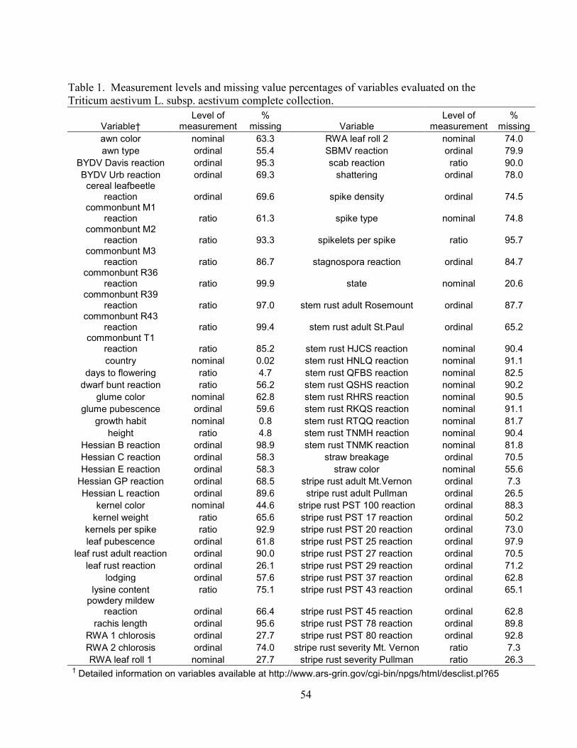
54
Table 1. Measurement levels and missing value percentages of variables evaluated on the
Triticum aestivum L. subsp. aestivum complete collection.
Variable† Level of
measurement %
missing Variable Level of
measurement %
missing
awn color nominal 63.3 RWA leaf roll 2 nominal 74.0
awn type ordinal 55.4 SBMV reaction ordinal 79.9
BYDV Davis reaction ordinal 95.3 scab reaction ratio 90.0
BYDV Urb reaction ordinal 69.3 shattering ordinal 78.0 cereal leafbeetle
reaction ordinal 69.6 spike density ordinal 74.5 commonbunt M1
reaction ratio 61.3 spike type nominal 74.8 commonbunt M2
reaction ratio 93.3 spikelets per spike ratio 95.7 commonbunt M3
reaction ratio 86.7 stagnospora reaction ordinal 84.7 commonbunt R36
reaction ratio 99.9 state nominal 20.6 commonbunt R39
reaction ratio 97.0 stem rust adult Rosemount ordinal 87.7 commonbunt R43
reaction ratio 99.4 stem rust adult St.Paul ordinal 65.2 commonbunt T1
reaction ratio 85.2 stem rust HJCS reaction nominal 90.4
country nominal 0.02 stem rust HNLQ reaction nominal 91.1
days to flowering ratio 4.7 stem rust QFBS reaction nominal 82.5
dwarf bunt reaction ratio 56.2 stem rust QSHS reaction nominal 90.2
glume color nominal 62.8 stem rust RHRS reaction nominal 90.5
glume pubescence ordinal 59.6 stem rust RKQS reaction nominal 91.1
growth habit nominal 0.8 stem rust RTQQ reaction nominal 81.7
height ratio 4.8 stem rust TNMH reaction nominal 90.4
Hessian B reaction ordinal 98.9 stem rust TNMK reaction nominal 81.8
Hessian C reaction ordinal 58.3 straw breakage ordinal 70.5
Hessian E reaction ordinal 58.3 straw color nominal 55.6
Hessian GP reaction ordinal 68.5 stripe rust adult Mt.Vernon ordinal 7.3
Hessian L reaction ordinal 89.6 stripe rust adult Pullman ordinal 26.5
kernel color nominal 44.6 stripe rust PST 100 reaction ordinal 88.3
kernel weight ratio 65.6 stripe rust PST 17 reaction ordinal 50.2
kernels per spike ratio 92.9 stripe rust PST 20 reaction ordinal 73.0
leaf pubescence ordinal 61.8 stripe rust PST 25 reaction ordinal 97.9
leaf rust adult reaction ordinal 90.0 stripe rust PST 27 reaction ordinal 70.5
leaf rust reaction ordinal 26.1 stripe rust PST 29 reaction ordinal 71.2
lodging ordinal 57.6 stripe rust PST 37 reaction ordinal 62.8
lysine content ratio 75.1 stripe rust PST 43 reaction ordinal 65.1 powdery mildew
reaction ordinal 66.4 stripe rust PST 45 reaction ordinal 62.8
rachis length ordinal 95.6 stripe rust PST 78 reaction ordinal 89.8
RWA 1 chlorosis ordinal 27.7 stripe rust PST 80 reaction ordinal 92.8
RWA 2 chlorosis ordinal 74.0 stripe rust severity Mt. Vernon ratio 7.3
RWA leaf roll 1 nominal 27.7 stripe rust severity Pullman ratio 26.3 † Detailed information on variables available at http://www.ars-grin.gov/cgi-bin/npgs/html/desclist.pl?65

55
Table 2. Removal percentages by variable for simulating data sets with missing values by
removing values from the "complete collection".
Level of
measurement
%
Variable Set 1 Set 2
country nominal 0 0
days to flowering ratio 5 95
height ratio 5 95
stripe rust adult Mt.Vernon ordinal 5 90
stripe rust severity Mt. Vernon ratio 5 90
state nominal 25 90
leaf rust reaction ordinal 25 90
RWA 1 chlorosis ordinal 25 75
RWA leaf roll 1 nominal 25 75
stripe rust adult Pullman ordinal 50 75
stripe rust severity Pullman ratio 50 75
kernel color nominal 50 50
Hessian C reaction ordinal 50 50
Hessian E reaction ordinal 75 50
kernel weight ratio 75 50
straw color nominal 75 25
awn type ordinal 75 25
lodging ordinal 90 25
leaf pubescence ordinal 90 25
glume color nominal 90 5
awn color nominal 90 5
straw breakage ordinal 95 5
commonbunt M1 reaction ratio 95 5

56
Table 3. Comparisons of core subset selection methods in terms of diversity of 1000 potential core subsets selected from 200
complete collections simulated with values removed at the rates given by set 1 (see Table 2) from accessions selected randomly from a
uniform distribution.
Core subset selection method RecMed† RecIQR† RecRange† RecNCat† RecH†
Distance Variables‡ Clustering§ Sampling¶
Mean # of accessions Medians# Ranks†† Medians Ranks Medians Ranks Medians Ranks Medians Ranks
Sparse UPGMA Logarithm 322.7 30.1 1.2 116.1 2.6 95.9 1.0 77.6 1.0 103.0 1.0
Sparse UPGMA Proportional 320.5 1.1 10.9 104.5 9.0 91.3 4.5 71.8 4.5 92.0 7.4
Sparse UPGMA Square Root 325.5 18.3 3.5 115.1 1.8 95.0 2.1 76.3 2.0 100.9 2.0
Sparse Ward Logarithm 340.2 6.0 6.5 112.0 3.7 90.4 5.9 71.0 5.7 94.9 4.9
Sparse Ward Proportional 310.0 4.2 6.8 102.8 11.1 89.2 11.0 68.2 11.4 90.3 11.2
Sparse Ward Square Root 330.0 1.5 8.1 110.6 5.3 90.1 7.2 70.2 7.0 93.6 6.0
Dense UPGMA Logarithm 314.3 25.2 1.8 110.7 5.3 92.5 3.3 72.6 3.8 98.7 3.0
Dense UPGMA Proportional 311.2 3.3 7.9 103.3 10.3 89.3 10.4 69.3 9.2 90.6 10.3
Dense UPGMA Square Root 327.4 15.7 4.4 112.8 3.2 91.8 4.5 72.2 4.3 96.4 4.1
Dense Ward Logarithm 339.7 0.9 9.4 109.3 6.4 89.8 8.1 69.5 8.3 91.8 7.7
Dense Ward Proportional 310.2 5.1 6.0 102.7 11.4 89.2 11.0 68.2 11.5 90.3 11.5
Dense Ward Square Root 329.9 0.7 11.5 106.8 8.0 89.6 9.0 69.1 9.4 91.3 9.0
† Recovery metrics: RecMed, recovery of median; RecIQR, recovery of interquartile range; RecRange, recovery of range; RecNCat, recovery of number of unique categories; RecH, recovery of Shannon's Index.
‡ Distance calculations were conducted using either all of the variables (Sparse) or only those few with 5% or less missing values (Dense).
§ Clustering of accessions methods: UPGMA, unweighted pair-group method using arithmetic averages; Ward, Ward’s minimum variance.
¶ Sampling accessions from each cluster in proportion to cluster size (proportional), natural logarithm of the size (logarithm), or square root of the size (square root).
# Means, over 200 simulations, of medians of recovery metrics of 1000 potential core subsets.
†† Means, over 200 simulations, of ranks of selection methods. Methods were ranked, with highest values receiving the lowest ranks, within each simulation based on medians, over 1000 potential core subsets, of recovery metrics.

57
Table 4. Comparisons of core subset selection methods in terms of diversity of 1000 potential core subsets selected from 200
complete collections simulated with values removed at the rates given by set 1 (see Table 2) from accessions selected as a contiguous
group.
Core subset selection method RecMed† RecIQR† RecRange† RecNCat† RecH†
Distance Variables‡ Clustering§ Sampling¶
Mean # of accessions Medians# Ranks†† Medians Ranks Medians Ranks Medians Ranks Medians Ranks
Sparse UPGMA Logarithm 314.4 27.0 2.1 122.3 2.2 95.2 1.4 75.4 2.0 101.7 1.2
Sparse UPGMA Proportional 317.4 0.9 11.1 104.0 9.2 91.0 5.1 70.8 5.9 91.6 8.0
Sparse UPGMA Square Root 325.6 13.0 4.5 115.9 2.7 94.5 2.1 74.7 2.0 99.4 2.2
Sparse Ward Logarithm 340.1 8.4 5.5 113.2 4.2 90.6 5.9 71.2 5.3 94.8 4.9
Sparse Ward Proportional 309.8 4.4 6.3 102.8 11.0 89.2 11.0 68.2 11.4 90.3 11.1
Sparse Ward Square Root 330.0 1.9 8.2 110.7 5.5 90.2 6.9 70.4 6.4 93.5 5.8
Dense UPGMA Logarithm 316.7 25.2 1.9 114.0 4.0 92.6 3.4 73.0 3.3 98.2 2.8
Dense UPGMA Proportional 310.9 3.8 7.0 102.9 10.6 89.3 10.6 68.9 9.5 90.4 10.6
Dense UPGMA Square Root 327.8 11.6 5.0 113.7 3.7 91.9 4.1 72.2 4.0 95.9 4.2
Dense Ward Logarithm 339.8 1.2 9.2 109.4 6.2 89.8 7.9 69.5 8.0 91.9 7.3
Dense Ward Proportional 310.2 4.8 5.9 102.7 11.1 89.2 11.1 68.2 11.3 90.3 11.2
Dense Ward Square Root 329.9 0.7 11.4 106.7 7.7 89.6 8.7 69.1 9.1 91.3 8.6
† Recovery metrics: RecMed, recovery of median; RecIQR, recovery of interquartile range; RecRange, recovery of range; RecNCat, recovery of number of unique categories; RecH, recovery of Shannon's Index.
‡ Distance calculations were conducted using either all of the variables (Sparse) or only those few with 5% or less missing values (Dense).
§ Clustering of accessions methods: UPGMA, unweighted pair-group method using arithmetic averages; Ward, Ward’s minimum variance. ¶ Sampling accessions from each cluster in proportion to cluster size (proportional), natural logarithm of the size (logarithm), or square root of the size (square root).
# Means, over 200 simulations, of medians of recovery metrics of 1000 potential core subsets. †† Means, over 200 simulations, of ranks of selection methods. Methods were ranked, with highest values receiving the lowest ranks, within each simulation based on medians, over 1000 potential core subsets, of recovery metrics.

58
Table 5. Comparisons of core subset selection methods in terms of diversity of 1000 potential core subsets selected from 200
complete collections simulated with values removed at the rates given by set 2 (see Table 2) from accessions selected randomly from a
uniform distribution.
Core subset selection method RecMed† RecIQR† RecRange† RecNCat† RecH†
Distance Variables‡ Clustering§ Sampling¶
Mean # of accessions Medians# Ranks†† Medians Ranks Medians Ranks Medians Ranks Medians Ranks
Sparse UPGMA Logarithm 315.4 4.3 4.7 114.1 1.2 89.8 7.0 74.1 1.5 99.7 1.1
Sparse UPGMA Proportional 312.2 6.0 3.6 103.0 9.3 89.4 7.4 70.4 7.2 90.8 9.2
Sparse UPGMA Square Root 325.8 1.4 7.3 111.3 3.3 90.1 4.1 73.7 2.1 97.1 2.5
Sparse Ward Logarithm 339.9 3.7 6.4 106.2 7.5 89.6 4.8 70.6 6.6 93.1 6.5
Sparse Ward Proportional 309.7 4.5 5.1 102.7 10.1 89.2 10.0 68.2 11.4 90.3 11.3
Sparse Ward Square Root 330.0 3.7 8.0 104.6 8.9 89.5 5.9 69.8 8.7 92.0 8.0
Dense UPGMA Logarithm 335.4 2.4 6.0 113.0 2.0 89.5 5.4 72.0 3.7 97.0 2.5
Dense UPGMA Proportional 310.5 6.2 3.4 102.9 9.6 89.2 10.0 70.5 7.0 90.5 9.9
Dense UPGMA Square Root 328.4 1.1 9.1 108.5 5.3 89.5 5.6 71.9 4.1 95.0 4.6
Dense Ward Logarithm 340.1 1.1 8.8 110.4 3.8 89.7 2.9 70.8 6.1 95.0 4.6
Dense Ward Proportional 309.7 4.7 4.5 102.7 10.3 89.2 9.8 68.2 11.5 90.3 11.5
Dense Ward Square Root 330.0 0.9 11.2 106.9 6.7 89.5 5.1 70.0 8.2 93.3 6.5
† Recovery metrics: RecMed, recovery of median; RecIQR, recovery of interquartile range; RecRange, recovery of range; RecNCat, recovery of number of unique categories; RecH, recovery of Shannon's Index.
‡ Distance calculations were conducted using either all of the variables (Sparse) or only those few with 5% or less missing values (Dense).
§ Clustering of accessions methods: UPGMA, unweighted pair-group method using arithmetic averages; Ward, Ward’s minimum variance.
¶ Sampling accessions from each cluster in proportion to cluster size (proportional), natural logarithm of the size (logarithm), or square root of the size (square root).
# Means, over 200 simulations, of medians of recovery metrics of 1000 potential core subsets.
†† Means, over 200 simulations, of ranks of selection methods. Methods were ranked, with highest values receiving the lowest ranks, within each simulation based on medians, over 1000 potential core subsets, of recovery metrics.
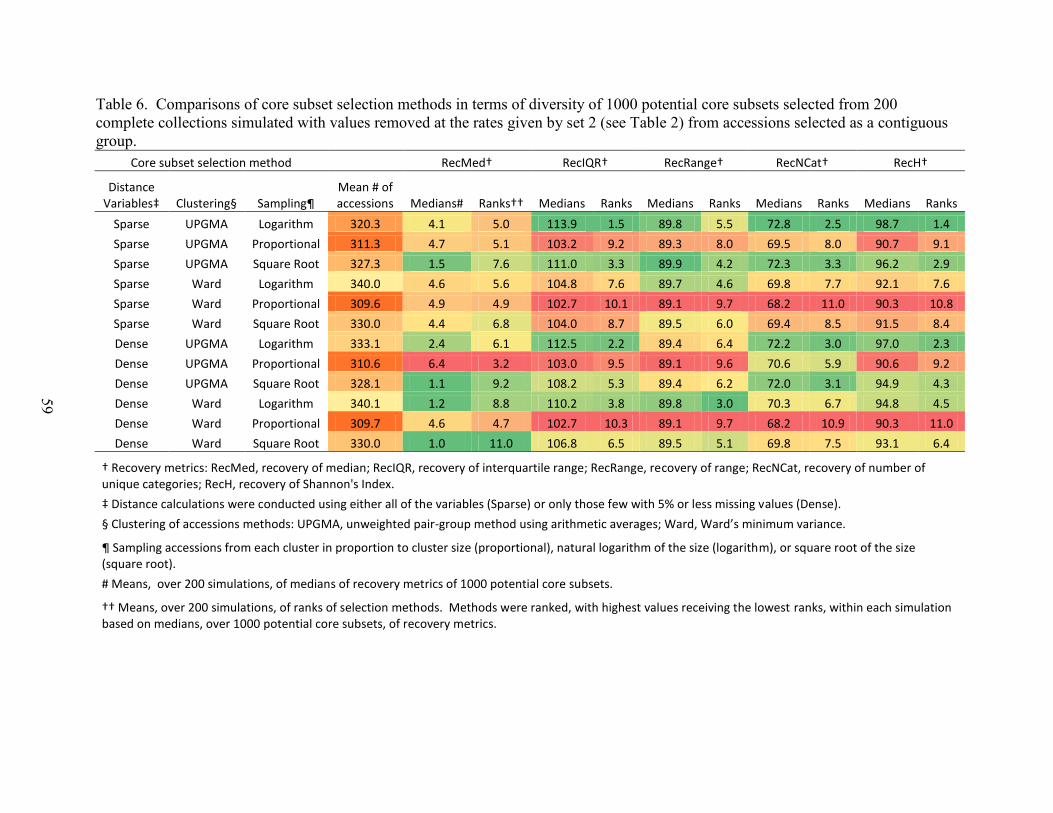
59
Table 6. Comparisons of core subset selection methods in terms of diversity of 1000 potential core subsets selected from 200
complete collections simulated with values removed at the rates given by set 2 (see Table 2) from accessions selected as a contiguous
group.
Core subset selection method RecMed† RecIQR† RecRange† RecNCat† RecH†
Distance Variables‡ Clustering§ Sampling¶
Mean # of accessions Medians# Ranks†† Medians Ranks Medians Ranks Medians Ranks Medians Ranks
Sparse UPGMA Logarithm 320.3 4.1 5.0 113.9 1.5 89.8 5.5 72.8 2.5 98.7 1.4
Sparse UPGMA Proportional 311.3 4.7 5.1 103.2 9.2 89.3 8.0 69.5 8.0 90.7 9.1
Sparse UPGMA Square Root 327.3 1.5 7.6 111.0 3.3 89.9 4.2 72.3 3.3 96.2 2.9
Sparse Ward Logarithm 340.0 4.6 5.6 104.8 7.6 89.7 4.6 69.8 7.7 92.1 7.6
Sparse Ward Proportional 309.6 4.9 4.9 102.7 10.1 89.1 9.7 68.2 11.0 90.3 10.8
Sparse Ward Square Root 330.0 4.4 6.8 104.0 8.7 89.5 6.0 69.4 8.5 91.5 8.4
Dense UPGMA Logarithm 333.1 2.4 6.1 112.5 2.2 89.4 6.4 72.2 3.0 97.0 2.3
Dense UPGMA Proportional 310.6 6.4 3.2 103.0 9.5 89.1 9.6 70.6 5.9 90.6 9.2
Dense UPGMA Square Root 328.1 1.1 9.2 108.2 5.3 89.4 6.2 72.0 3.1 94.9 4.3
Dense Ward Logarithm 340.1 1.2 8.8 110.2 3.8 89.8 3.0 70.3 6.7 94.8 4.5
Dense Ward Proportional 309.7 4.6 4.7 102.7 10.3 89.1 9.7 68.2 10.9 90.3 11.0
Dense Ward Square Root 330.0 1.0 11.0 106.8 6.5 89.5 5.1 69.8 7.5 93.1 6.4
† Recovery metrics: RecMed, recovery of median; RecIQR, recovery of interquartile range; RecRange, recovery of range; RecNCat, recovery of number of unique categories; RecH, recovery of Shannon's Index.
‡ Distance calculations were conducted using either all of the variables (Sparse) or only those few with 5% or less missing values (Dense).
§ Clustering of accessions methods: UPGMA, unweighted pair-group method using arithmetic averages; Ward, Ward’s minimum variance.
¶ Sampling accessions from each cluster in proportion to cluster size (proportional), natural logarithm of the size (logarithm), or square root of the size (square root).
# Means, over 200 simulations, of medians of recovery metrics of 1000 potential core subsets.
†† Means, over 200 simulations, of ranks of selection methods. Methods were ranked, with highest values receiving the lowest ranks, within each simulation based on medians, over 1000 potential core subsets, of recovery metrics.
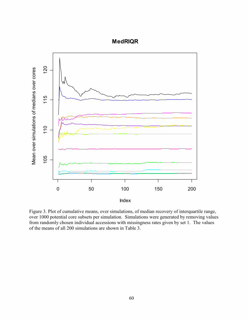
60
Figure 3. Plot of cumulative means, over simulations, of median recovery of interquartile range,
over 1000 potential core subsets per simulation. Simulations were generated by removing values
from randomly chosen individual accessions with missingness rates given by set 1. The values
of the means of all 200 simulations are shown in Table 3.
0 50 100 150 200
10
51
10
11
51
20
MedRIQR
Index
Me
an
ove
r sim
ula
tio
ns o
f m
ed
ian
s o
ve
r co
res

61
Figure 4. Plot of cumulative means, over simulations, of median recovery of interquartile range,
over 1000 potential core subsets, ranked across methods within each simulation. Simulations
were generated by removing values from randomly chosen individual accessions with
missingness rates given by set 1. The mean ranks, over all 200 simulations, are shown in Table
3.
0 50 100 150 200
02
46
81
01
2RRIQR
Index
Me
an
of R
an
ks

62
Appendix Table 1. Assignments of countries to world macro region components.
Carribean Central America South America Northern America Eastern Asia South-Central Asia
South-eastern Asia
Cuba Guatemala Argentina Canada China Afghanistan Indonesia
Honduras Bolivia United States Japan Bangladesh Philippines
Mexico Brazil
Korea, North Bhutan Thailand
Nicaragua Chile
Korea, South India
Panama Colombia
Mongolia Iran
Ecuador
Taiwan Kazakhstan
Paraguay
Kyrgyzstan
Peru
Nepal
Uruguay
Pakistan
Venezuela
Tajikistan
Turkistan
Turkmenistan
Uzbekistan
Western Asia Eastern Europe Northern Europe Southern Europe
Western Europe Oceania Unknown
Ancient Palestine Belarus Denmark Albania Austria Australia Asia
Armenia Bulgaria Estonia Andorra Belgium New Zealand Europe
Asia Minor Czech Republic Finland Bosnia and Herzegovina France
Uncertain
Azerbaijan Czechoslovakia Iceland Croatia Germany
Unknown
Cyprus Former Soviet Union Ireland Former Yugoslavia Netherlands Georgia Hungary Latvia Greece Switzerland Iraq Moldova Lithuania Italy
Israel Poland Norway Macedonia
Jordan Romania Sweden Malta
Lebanon Russian Federation United Kingdom Portugal
Oman Slovakia
Slovenia
Saudi Arabia Ukraine
Spain
Syria
Yugoslavia
Turkey
Yemen

63
Appendix Table 2. Comparison of original core subset against the reselected core subset in
terms of recovery metrics.
Core Subset RecMed† RecIQR† RecRange† RecNCat† RecH†
Original 4.0 101.5 97.7 92.5 101.0 New core 9.2 95.8 98.2 94.9 109.3
† Recovery metrics: RecMed, recovery of median; RecIQR, recovery of interquartile range; RecRange, recovery of range; RecNCat, recovery of number of unique categories; RecH, recovery of Shannon's Index.

64
CHAPTER 3
COMPARISON OF LINEAR MIXED MODELS FOR MULTIPLE
ENVIRONMENT PLANT BREEDING TRIALS
Carl A. Walker1, Fabiano Pita
2, Kimberly Garland Campbell
1,3
1 Dept. of Crop and Soil Sciences, Washington State University;
2 Quantitative Genetics Group, Dow
AgroSciences; 3 USDA-ARS, Wheat Genetics, Quality, Physiology, and Disease Research Unit
Abstract
Evaluations of genotypes in varied environmental conditions are referred to as multiple environment trials
(MET) and often show genotype by environment interactions, necessitating estimation of effects of
genotypes within environments. Empirical best linear unbiased predictions can provide more accurate
estimates of these effects, depending upon the mixed model used. The objective of this work was to
simulate and analyze MET data sets to determine which linear models provide the most accurate
estimates and determine how the choice of ideal model changes as a result of different MET conditions.
Simulations varied in terms of numbers of genotypes and environments, variances and covariances of
genotype responses within and between environments, experimental design, and experimental error
variance. Simulated MET were fit with mixed models with or without genetic relationship matrices
(GRM) and with structures of varying complexity used to model relationships among environments.
Estimates from these analyses for effects of genotypes within environments were compared to the
simulated values. The model that included a GRM and constant variance-constant correlation structure
was the most accurate for the largest number of scenarios. Models including GRM that allowed
heterogeneous environmental variances with constant correlations often resulted in greater accuracy when
MET were simulated with heterogeneous variances among environments. Factor analytic models with
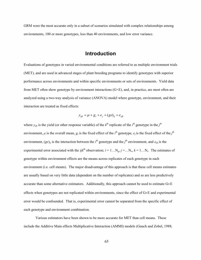
65
GRM were the most accurate only in a subset of scenarios simulated with complex relationships among
environments, 100 or more genotypes, less than 40 environments, and low error variance.
Introduction
Evaluations of genotypes in varied environmental conditions are referred to as multiple environment trials
(MET), and are used in advanced stages of plant breeding programs to identify genotypes with superior
performance across environments and within specific environments or sets of environments. Yield data
from MET often show genotype by environment interactions (G×E), and, in practice, are most often are
analyzed using a two-way analysis of variance (ANOVA) model where genotype, environment, and their
interaction are treated as fixed effects:
where yijk is the yield (or other response variable) of the kth replicate of the i
th genotype in the j
th
environment, μ is the overall mean, gi is the fixed effect of the ith genotype, ej is the fixed effect of the j
th
environment, (ge)ij is the interaction between the ith genotype and the j
th environment, and ijk is the
experimental error associated with the ijkth observation; i = 1…Ng, j =…Ne, k = 1…Nr. The estimates of
genotype within environment effects are the means across replicates of each genotype in each
environment (i.e. cell means). The major disadvantage of this approach is that these cell means estimates
are usually based on very little data (dependent on the number of replicates) and so are less predictively
accurate than some alternative estimators. Additionally, this approach cannot be used to estimate GE
effects when genotypes are not replicated within environments, since the effect of GE and experimental
error would be confounded. That is, experimental error cannot be separated from the specific effect of
each genotype and environment combination.
Various estimators have been shown to be more accurate for MET than cell means. These
include the Additive Main effects Multiplicative Interaction (AMMI) models (Gauch and Zobel, 1988;
ijkijjiijk geegy )(

66
Gauch, 1988) and sites regression (SREG; Cornelius and Crossa, 1999) model families, which are
sometimes referred to as linear-bilinear models. These two fixed-effect model families include sums of
multiplicative terms, resulting from singular value decomposition, replacing (ge)ij, in the case of AMMI,
or gi +(ge)ij for SREG. The AMMI and SREG models have been shown to be relatively equivalent in
terms of predictive accuracy (Cornelius and Crossa, 1999). Like the analysis of G×E in a fixed-effects
ANOVA, the standard implementation of these models cannot be used when data from any genotype and
environment combination is missing. However, the expectation-maximization algorithm has been used to
impute missing data with the AMMI model (Gauch and Zobel, 1990).
As an alternative to the above models that consider genotype effects within environments as
fixed, these effects can be considered random values and modeled using linear mixed models, which have
important inherent benefits over fixed-effects models. Mixed models can easily incorporate non-constant
error variance structures, including within-field spatial correlation, in the same model as genotype and
environment effects. Additionally, mixed models easily handle missing data and, with some specific
models, even unreplicated data. Some models can predict genotype effects in environments they were not
tested in.
Mixed model analyses have a long history in animal breeding (Henderson, 1973), and recent
research has demonstrated new approaches to make them very effective in plant breeding. If a mixed
linear model is used, genotype effects are estimated as empirical best linear unbiased predictors (BLUPs)
calculated using the estimated variance parameters. A very basic mixed model would assume a random
effect of genotypes within environments that has a variance-covariance matrix of σ2I, where σ
2 is a
constant variance parameter and I is an identity matrix. In most breeding programs, plant or animal, at
least a portion of the genotypes assessed in a trial are related and therefore would be expected to show
some correlation in their effects. Pedigree information can be incorporated into the model through a
Genetic Relationship Matrix (GRM) to take advantage of these relationships and improve predictive
accuracy (Henderson, 1973). The GRM is also known as the additive relationship matrix, or numerator
relationship matrix and is usually symbolized as A, and A = 2[fii′], where fii′ is the coefficient of parentage
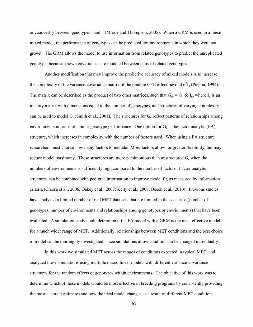
67
or coancestry between genotypes i and i′ (Mrode and Thompson, 2005). When a GRM is used in a linear
mixed model, the performance of genotypes can be predicted for environments in which they were not
grown. The GRM allows the model to use information from related genotypes to predict the unreplicated
genotype, because known covariances are modeled between pairs of related genotypes.
Another modification that may improve the predictive accuracy of mixed models is to increase
the complexity of the variance-covariance matrix of the random G×E effect beyond σ2Ig (Piepho, 1994).
The matrix can be described as the product of two other matrices, such that Gge = Ge ⨂ Ig, where Ig is an
identity matrix with dimensions equal to the number of genotypes, and structures of varying complexity
can be used to model Ge (Smith et al., 2001). The structures for Ge reflect patterns of relationships among
environments in terms of similar genotype performance. One option for Ge is the factor analytic (FA)
structure, which increases in complexity with the number of factors used. When using a FA structure
researchers must choose how many factors to include. More factors allow for greater flexibility, but may
reduce model parsimony. These structures are more parsimonious than unstructured Ge when the
numbers of environments is sufficiently high compared to the number of factors. Factor analytic
structures can be combined with pedigree information to improve model fit, as measured by information
criteria (Crossa et al., 2006; Oakey et al., 2007; Kelly et al., 2009; Beeck et al., 2010). Previous studies
have analyzed a limited number of real MET data sets that are limited in the scenarios (number of
genotypes, number of environments and relationships among genotypes or envrionments) that have been
evaluated. A simulation study could determine if the FA model with a GRM is the most effective model
for a much wider range of MET. Additionally, relationships between MET conditions and the best choice
of model can be thoroughly investigated, since simulations allow conditions to be changed individually.
In this work we simulated MET across the ranges of conditions expected in typical MET, and
analyzed these simulations using multiple mixed linear models with different variance-covariance
structures for the random effects of genotypes within environments. The objective of this work was to
determine which of these models would be most effective in breeding programs by consistently providing
the most accurate estimates and how the ideal model changes as a result of different MET conditions.

68
Methods
Simulations
Simulations were conducted to generate data sets that resemble MET across a range of conditions. The
simulations included randomly generated effects of genotypes within environments and phenotypes of
each observation, resulting from the addition of a random experimental error to the genotype within
environment effect. These simulated data sets covered a range of scenarios with varying numbers of
environments and genotypes, environmental relationship patterns, field trial designs, and magnitudes of
experimental error.
Genotype effects within each environment were simulated as random samples from multivariate
normal distributions with means of 0 and covariance matrices (ΣGE) that differed among scenarios. The
ΣGE are equivalent to correlation matrices multiplied by a constant scalar variance component of unity.
The ΣGE were the Kronecker (or direct) product of a matrix of correlations between environments (ΣE) and
a matrix of correlations between genotypes (ΣG). The ΣE were generated in four sizes: 5 × 5, 10 × 10, 20
× 20, and 40 × 40, corresponding to scenarios with 5, 10, 20, or 40 environments, respectively. The ΣE
were themselves generated as Kronecker products of two matrices: EY ⨂ EL. The ΣE matrices for five
and ten environments were simply products of EL matrices of size 5 × 5 or 10 × 10 with a 1 × 1 EY matrix
of unity, whereas the ΣE of 20 and 40 environments were Kronecker products of 4 × 4 and 8 × 8 EY
matrices with a 5 × 5 EL matrix. This allows the ΣE to better reflect possible complex patterns of
relationships among large numbers of environments. For example, the five and ten environment scenarios
reflect MET with five or ten locations in a single year, whereas the 20 and 40 environment scenarios
reflect MET with five locations evaluated over four or eight years.
The ΣE are grouped into three classes of patterns of correlations: compound symmetry A (CSA),
compound symmetry B (CSB), and Toeplitz (Toep). For the compound symmetric classes both the EY
and EL matrices had constant off-diagonal elements of 0.3 and 0.7 for CSA and 0.4 and 0.4 for CSB. Both

69
the EY and EL matrices for the Toeplitz class of patterns had bands of constant correlation parallel to the
diagonal with the greatest correlations next to the diagonal. The exact correlations differed by the sizes of
ΣE, but in all cases included negative values for the element farthest from the diagonal. These specific
correlation values are by no means the only correlation values that could occur in a MET, but were
chosen to be similar to values observed in the Washington State University soft white wheat variety trials
(details provided in the appendix).
The EL were generated with three levels of variance heterogeneity: homogeneous variances (CSA,
etc.), heterogeneous variances (CSAH, etc.), and very heterogeneous variances (CSAVH, etc.). To do so,
the EL were pre and post multiplied by a diagonal matrix of standard deviations. For the heterogeneous
variances the variances ranged from 0.5 to 1.5 for the least and greatest variances, respectively. The very
heterogeneous variances ranged from 0.2 to 2. The three to one ratio is often used as a rule-of-thumb
cutoff for considering variances to be heterogeneous, but greater levels of heterogeneity can occur among
highly variable environments.
Four options were considered for ΣG, corresponding to scenarios of 25, 50, 100, and 150
genotypes. In order to choose ΣG, first a GRM was estimated from the pedigree in a Dow AgroSciences
early generation study of North American Stiff Stalk maize inbred lines. The four options were
overlapping submatrices of this GRM: the first 25, 50, 100, and 150 rows and columns in the GRM.
With four options for sizes of ΣE, three classes of patterns for ΣE, three levels of variance
heterogeneity, and four options for ΣG, taking all combinations results in a total of 144 different simulated
scenarios for ΣGE. For each ΣGE, genotype effects were generated by randomly sampling from a
multivariate normal distribution with variance-covariance matrix equal to ΣGE 1000 times.
For each set of genotype within environment effects, simulations were generated for three trial
designs (RCBD – randomized complete block designs, MAD – modified augmented designs, and
unreplicated designs) and two experimental error variances. Since spatial field effects were not
considered, the only effect of the experimental design was to determine the number of replicates of each
genotype in each environment. Therefore, other designs commonly used in MET will also have either

70
equal or unequal replication, regardless of blocking structure, and so would not add much beyond the
designs tested here. For the RCBD scenarios, every genotype was replicated three times. In the MAD
scenarios, genotypes were not replicated except for primary and secondary “checks” that were replicated
five and two times, respectively, for every 23 non-check genotypes. In the unreplicated design, each
genotype appeared once in each environment. A fixed effect for each environment was simulated by
sampling one value from a gamma (3, 2) distribution and multiplying it by 3. This distribution and
constant multiplier were chosen to provide environment effects that are of similar magnitude to the
simulated genotype effects and error. Every observation had a unique phenotype equal to the effect of the
genotype in an environment plus a simulated environment effect and a random experimental error
selected from a normal distribution with mean of 0 and two possible error variances (σe2 = 0.5 or 2.0).
These error variances corresponded to ratios of about 1.7 and 0.4, respectively, of variance of the
genotype within environment effects divided by the variance of the experimental error for a given
simulation. The ratios values varied slightly around these averages among scenarios with greater values
for scenarios with more environments.
Analyses
A total of 20 related linear mixed models were compared for their ability to predict the simulated
genotype effects within environments based on the simulated phenotypic data. Models were fit using the
program ASReml-R, release 3.0 (Butler et al., 2009), which is a package for the R programming language
(R Development Core Team, 2010). The models were all of the form:
,
where y is the vector of observed phenotypes, β is a vector of fixed environment effects, X is the
associated design matrix, γ is the vector of genotype within environment effects, Z is the associated
design matrix, and ε is the vector of experimental error terms. The joint distribution of γ and ε is given
by:
εZγXβy

71
,
where is a constant error variance and G is a covariance structure that varies for each of the 20
models and is separable:
G = GE ⨂ B,
where both GE and B were varied, resulting in 20 models:
B = I or A,
where I is an identity matrix and A is a GRM. This study evaluated the ideal situation, when the GRM
used perfectly reflects the actual relationships among the genotypes; therefore, A was set equal to the ΣG
used to simulate of the data set being analyzed.
Ten structures were used to model GE and these are shown below for a five environment
example. The simplest structure was independence (no covariance) and identical variances (ID):
.
A generalization of this is the diagonal structure, where environments are still independent, but each can
have different variance (Diag):
.
A constant covariance can be added, yielding compound symmetric structures with uniform (CorV) or
heterogeneous variances (CorH):
I0
0G
0
0
ε
γ2
,MVN~R
2R
2
2
2
2
2
0000
0000
0000
0000
0000
EG
25
24
23
22
21
0000
0000
0000
0000
0000
EG

72
.
Six FA structures were compared. Structures were fit with one to three factors and uniform or
heterogeneous specific variances (FA1U, FA2U, FA3U, FA1H, FA2H, FA3H):
GE = ΛΛ′ + Ψ,
where Λ is a matrix whose columns are the factors and Ψ is a diagonal matrix of specific variances:
In an effort to improve convergence rates, models were fit sequentially in the order of the GE
structures described above. Parameter estimates from simpler models were used as the starting values of
the next more complex structure for which the simple structure was a specific case. If a model did not
converge, the next more complex structure was not attempted. The percentage of simulations of a
scenario for which a model converged was defined as the convergence rate.
In addition to the mixed linear models, estimates of genotype effects within environments were
derived from cell means (the mean of the replicates of a genotype in each environment) and Additive
Main effects Multiplicative Interaction (AMMI) models. The AMMI models were fixed effects linear
models with main effects for genotype and environment. The effects of genotype by environment
interaction were replaced with an approximation of the matrix using a reduced set of the principle
211111
12
1111
112
111
1112
11
11112
1
EG
2511111
1241111
1123111
1112211
1111211
EG
53
43
33
23
13
52
42
32
22
12
51
41
31
21
11
52
42
32
22
12
51
41
31
21
11
51
41
31
21
11
or,,
Λ
5
4
3
2
1
5
0000
0000
0000
0000
0000
or
IΨ

73
components (Gauch, 1988). Only RCBD scenarios were analyzed using the AMMI models, since main
effects of genotype and environment cannot be separated from the interaction term if genotypes are not
replicated in an environment. The AMMI models were fit with all possible numbers of principle
components. The most accurate of the AMMI models for each simulation, as judged by the root mean
square error of prediction (described below), were compared to the mixed linear models. However, this
was often not the most accurate AMMI model as measured with the correlations between estimates from
the model and the simulated data.
To evaluate each model‟s predictive accuracy, Pearson and Spearman correlations between the
estimated effects of genotypes within environments and the simulated effects were calculated for each
simulation. Additionally, root mean squared errors of prediction (RMSEP) were calculated as:
, where p is the number of genotype by environment combinations, γi is the
ith effect of a genotype within an environment, and is the i
th predictor. Both the Akaike and Bayesian
information criteria (AIC and BIC, respectively) were also calculated for each of the mixed models. The
models were ranked based on each of these accuracy measures and the information criteria within each
simulation. Models that were not fit or did not fit were all given the same rank value just inferior to the
least accurate. The accuracy measurements for each model varied greatly among simulations of the same
scenario, whereas the rankings varied to a lesser degree. In order to summarize the results for each
scenario, means were taken, over simulations, of the accuracy measurements and the rankings of the
models.
For each scenario, a different number of simulations were analyzed with every model to ensure
that sufficient simulations were analyzed to produce reliable means. Simulations were analyzed
sequentially, and following the analysis of each simulation, rankings of RMSEP, Pearson correlations,
and Spearman correlations were averaged over the analyzed simulations. When these three cumulative
mean rankings did not change by more than 0.05 one simulation to the next or over 10 simulations, no
p
ip
2
ii γγ~1
RMSEP
iγ~

74
additional simulations were analyzed for that scenario. The number of simulations necessary to achieve
this stability varied greatly among scenarios. Due to time constraints, the scenarios with the largest data
sets were not analyzed and do not appear in the results.
Results and Discussion
Justification of Approach
Since the simulations within each scenario were all random realizations of MET described by the
scenario, no particular simulation was more valid than the others and a mean over all the simulations is a
valid summary of model performance for a given scenario. A model can be considered to be the best for
a given scenario if it has the greatest accuracy averaged over all simulations. However, using mean
accuracy excessively weights performance in simulations that result in extremely low or high accuracy for
a given model. Alternatively, the best model might be defined as one that has the greatest accuracy in the
most simulations. To evaluate this, model accuracy can be ranked within each simulation, and the mean
of the ranks for each model calculated. High accuracy values for a given simulation have no additional
influence if the model is already top ranked, but an occasional low ranking can still pull the mean rank
down. This approach rewards models that perform well consistently rather than those with inconsistent
extraordinary performance. This was the approach that we took to summarize our results. Models were
ranked with '1' being the best rank and a greater number indicating worse performance. The mean values
and ranks of all accuracy measurements for each model and scenario are given in Supplemental Table 1.
Results from RMSEP, Pearson correlations, and Spearman correlations differ, but conclusions as
to the best model were generally consistent after averaging over simulations. Results from the
information criteria were highly variable among simulations. Additionally, with our simulation approach,
the “true” simulated effects of genotypes within environments were available, allowing for direct
comparison of the simulated and estimated values. Therefore, the information criteria were of limited
value. The Spearman correlations may be more applicable than the Pearson from the perspective of

75
breeding, since genotypes are often selected based on their rankings, rather than observed values.
However, ranking of genotypes is not the only use of estimates of genotype responses in different
environments. Since these estimates are also used to evaluate traits like stability, the deviations of
estimates from the true values may be more important than how well the ranks agree. The accuracy
measured by RMSEP reflects how much estimates deviated from the simulated values, penalizing more
extreme values to a greater extent. This was desirable, as extreme errors in estimation are more likely to
cause rank changes among genotypes, leading to changes in selection decisions. In the interest of brevity,
we limit our discussion to RMSEP accuracy. The important conclusions from these data are summarized
below along with illustrative graphs of the data.
Choice of a Default Model
The plot of the mean ranks, in terms of RMSEP, for each model in each scenario showed that the
model with the genetic relationship matrix and a constant variance-constant correlation structure
(GRM_CorV) was the best model in many, but not all, situations (Figure 1). When the mean rankings of
the models were graphed, there was a pattern of nine troughs that correspond to the scenarios with the
fewest environments (Figure 1). In these scenarios the mean ranking of the best model was a greater
number. This indicates that there was less consistency in the top model rankings among simulations.
That is, the best model was not ranked first in all simulations of a scenario, or even necessarily always in
the top three. However, no other model did as well overall. Because of this pattern, in order to better
visualize the best model for each scenario, we graphed the results by ranking the means of the ranks for
each scenario. This standardized the graph in Figure 1, so that the best model was in the top row in each
scenario (Figure 2). The top row was predominantly GRM_CorV or GRM_CorH. To simplify even
more, we graphed results from just the GRM_CorV and GRM_CorH models (Figure 3). The points in the
top row indicate which of GRM_CorV or GRM_CorH was the best model for a scenario, whereas blanks
in the top row indicate that a model other than these two was the best for a scenario. Generally, the
GRM_CorV model appears to be a good default choice of model, i.e. if one decided which model to use

76
without additional specific information about a MET, since it was often the best ranked model and was
always in the top 10 models.
Models for Specific Scenarios
When all scenarios were examined together, it was difficult to determine if there were any
patterns as to when GRM_CorV, GRM_CorH, or another model was the best, but subsets of scenarios
allowed such evaluations. The GRM_CorV model was the most accurate model in most scenarios with
high error variance, whereas the GRM_CorH model was superior in few scenarios and the other models
were best only rarely (Figure 4). The GRM_CorV was preferred in fewer of the scenarios with low error
variance (Figure 5). In these scenarios the GRM_CorH and other models were the best in more cases.
These results indicate that as plot-to-plot error in a MET increases, the effectiveness of complex models
for GE decreases. The increased noise resulted in inaccurate estimation of the many parameters in the
complex models. In contrast, the CorV and CorH structures more accurately estimated fewer parameters,
compensating for their oversimplification of the pattern of relationships among environments.
One would expect that the GE structure in the most accurate model would be of similar
complexity to the pattern used to simulate relationships among environments. While such relationships
occurred, they were not entirely predictive. The GRM_CorV model was the best choice in almost all
scenarios simulated with a compound symmetric pattern for GE (Figure 6). This was to be expected,
since the CorV structure exactly matched the simulated pattern for five or 10 environments, and with 20
or 40 environments the simulated pattern only had two possible values that did not dramatically differ
from each other. In the scenarios simulated with compound symmetric correlation patterns and
heteroskedasticity, one might expect the CorH structure to be the best choice. However, it was only
superior to the CorV structure in some scenarios (Figure 7). An explanation for this is that the CorH
structure traded parsimony for flexibility, and in doing so, increased the risk that it modeled noise rather
than capturing actual differences in variances. Since the variance heterogeneity was not especially large
in these scenarios, there were many occasions where the ability to model this heterogeneity was not
valuable. With compound symmetric scenarios that include very heterogeneous environmental variances,

77
the GRM_CorH was generally the best, losing out to other models only in a small number of cases
(Figure 8). With these scenarios it was more important to model the greater degree of heterogeneity.
When scenarios were simulated with Toeplitz patterns the GRM_CorV and GRM_CorH models
were still generally the best, with GRM_CorH more often superior as heteroskedasticity increased (Figure
9). Models other than GRM_CorV or GRM_CorH were superior in scenarios with Toeplitz patterns, 100
or more genotypes, less than 40 environments, and low error variance (Figure 10). In these scenarios, one
of the models with a GRM and FA structures was almost always superior to the GRM_CorV or
GRM_CorH. This was also true with either 50 genotypes or a high error variance (not both) if a RCBD
was used (not shown). Unfortunately, prediction of error variance and patterns of relationships among
environments is difficult, especially due to dramatic year-to-year variability.
The number of genotypes, the number of environments in which they were tested, and the
replication as determined by the experimental design had limited effect on the choice of the best model.
When only 25 genotypes are included, the GRM_CorV model was preferred over the GRM_CorH and
other models in most scenarios (Figure 11). Complex relationships in genotype performance among
environments were not influential with so few genotypes. Therefore, it was better to just assume constant
correlations of genotype performance among environments. The GRM_CorH and more complex models
were more frequently ranked better than GRM_CorV as the number of genotypes increased. The reverse
pattern was true for numbers of environments. As the number of environments was increased, the
effectiveness of the more complex models decreased. In the MET simulations, the overall range of
correlations between pairs of environments was about the same (0.7 to -0.1 for 5 and 10 environments and
0.75 to 0.2 for 20 and 40 environments) for all numbers of environments. As the number of environments
was increased, the differences among the correlation parameters decreased resulting in many correlation
parameters with similar values, and reducing the benefits of having large numbers of parameters in the
model. Such a constraint on the correlations is also likely in reality, unless the large number of
environments cover a wider geographic or temporal range that would extend the range of possible
correlations beyond those tested here.
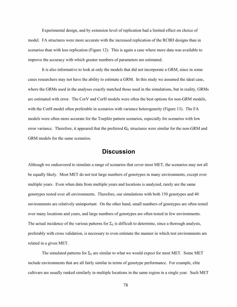
78
Experimental design, and by extension level of replication had a limited effect on choice of
model. FA structures were more accurate with the increased replication of the RCBD designs than in
scenarios than with less replication (Figure 12). This is again a case where more data was available to
improve the accuracy with which greater numbers of parameters are estimated.
It is also informative to look at only the models that did not incorporate a GRM, since in some
cases researchers may not have the ability to estimate a GRM. In this study we assumed the ideal case,
where the GRMs used in the analyses exactly matched those used in the simulations, but in reality, GRMs
are estimated with error. The CorV and CorH models were often the best options for non-GRM models,
with the CorH model often preferable in scenarios with variance heterogeneity (Figure 13). The FA
models were often more accurate for the Toeplitz pattern scenarios, especially for scenarios with low
error variance. Therefore, it appeared that the preferred GE structures were similar for the non-GRM and
GRM models for the same scenarios.
Discussion
Although we endeavored to simulate a range of scenarios that cover most MET, the scenarios may not all
be equally likely. Most MET do not test large numbers of genotypes in many environments, except over
multiple years. Even when data from multiple years and locations is analyzed, rarely are the same
genotypes tested over all environments. Therefore, our simulations with both 150 genotypes and 40
environments are relatively unimportant. On the other hand, small numbers of genotypes are often tested
over many locations and years, and large numbers of genotypes are often tested in few environments.
The actual incidence of the various patterns for ΣE is difficult to determine, since a thorough analysis,
preferably with cross validation, is necessary to even estimate the manner in which test environments are
related in a given MET.
The simulated patterns for ΣE are similar to what we would expect for most MET. Some MET
include environments that are all fairly similar in terms of genotype performance. For example, elite
cultivars are usually ranked similarly in multiple locations in the same region in a single year. Such MET

79
would have an underlying pattern of environmental relationships similar to a compound symmetric
pattern. MET that include environments that are very dissimilar to the others tested, may be more
common. This might occur when a MET includes one year when the weather was different than normal.
The Toeplitz patterns for ΣE provide a wide range of correlations, including negative values.
One might argue that our simulations should have included scenarios with independence among
environments; however, when modeling genotype effects within environments (without fixed genotype
effects), independence would only occur if genotype performance in one environment had no relationship
to performance in another. This independence would only occur in reality if the environments tested in
had completely different climates and/or the genotypes tested only differed in terms of specific response
to those environments.
Other researchers have previously compared the same mixed models as in this study, usually fit to
real data sets. Their results generally match ours for the most closely matching simulations. Piepho
(1998) observed that, for five MET, empirical BLUPs based on factor analytic structures were more
accurate than least squares estimates of cell means and usually better than predictions from unstructured
covariance matrices. We also saw greater accuracy from factor analytic models than the cell means.
Crossa et al. (2006) evaluated a wide range of mixed linear models on a single wheat MET with
29 genotypes, 16 locations throughout the world, and a RCBD with three replicates. These researchers
concluded that a nine factor, heterogeneous specific variance, factor analytic model with a GRM derived
from a pedigree, best fit the data as measured by various information criteria. The factor analytic model
was superior to a range of models including those with constant environmental correlation. The trial they
analyzed is most comparable to our scenarios with 25 genotypes, 10 or 20 environments, and RCBD
designs. For these scenarios, we did not find that FA structure models with GRM were superior to
GRM_CorV or GRM_CorH models as measured by average RMSEP ranking. However, rankings of the
models based on information criteria scores were highly variable among simulations, suggesting that our
differences in conclusions may be due to the chance conditions specific to the single trial investigated by
Crossa et al.

80
Other researchers have also found that FA models resulted in better AIC scores than simpler or
more complex structures when fit to real data sets (Kelly et al., 2007; Oakey et al., 2007; Beeck et al.,
2010). Kelly et al. (2007) also used RMSEP values from the analysis of simulated MET to show that FA
or unstructured environmental covariance models were superior to constant correlation models, but did
not evaluate GRM. These authors all evaluated real or simulated data sets which included relatively large
numbers of genotypes, and their results agreed with ours for simulations with 100 or more genotypes with
Toeplitz patterns for ΣE. It is likely that the sets of environments these researchers evaluated had complex
relationship patterns similar to our Toeplitz patterns and the simulations of Kelly et al. had heterogeneous
environmental correlations, making them similar to our Toeplitz patterns.
So and Edwards (2011) evaluated 51 maize MET, each with 6 environments (two years) and 187
to 386 genotypes only partially overlapping between years. They fit these 51 with mixed models that did
not include GRM and included various environmental covariance matrices for five of the six
environments, and performance was predicted in the sixth environment for purposes of cross validation.
These authors found that models that allowed for heterogeneous genetic covariances were often inferior to
compound symmetric models, in agreement with our results from simulations.
Our study and those of other researchers have generally focused on model fit or predictive
accuracy of empirical BLUPs, but MET are also analyzed to estimate relationships among environments.
Identification of highly correlated environments allows researchers to save resources by avoiding
redundant locations. Alternatively, information about highly unrelated environments can aid
interpretation of results from these esoteric locations or years. Although our analyses indicated that
simpler models often provided more accurate estimates, a simple structure for GE does not allow the
estimation of different parameters (variances or covariances) for different environments. In situations
where it is important to estimate these differences, factor analytic structures are preferable even if some
accuracy is sacrificed.
Conclusions

81
The most accurate models for analyzing MET always included a GRM, but differed among simulated
scenarios in terms of the ideal GE structure for estimating relationships in genotype performance among
environments. Complex structures that allow for heterogeneity of environmental variances or correlations
were only successful when the pattern used to simulate the data also had heterogeneous variances or
correlations. Even when this was true, if error variance was high or the MET had few genotypes, simpler
models were often more accurate. These results suggest that while GRM should be used when available,
complex structures for environmental relationships, such as FA, should only be used when evaluating 100
or more genotypes and a complex underlying structure is expected along with low error variance.
Appendix: Real Data as a Basis for Simulations
A simulation study is only effective if the simulations reflect the actual conditions that are being
simulated. Obviously, the actual biology of MET is more complex than our simulations, but a properly
tuned simulation should be able to approximate actual MET data. In order to create simulations that
effectively reflect actual MET in breeding programs, the parameters used in our simulations were chosen
based on the analysis of real MET.
Yield data from Washington State University soft white wheat variety improvement trials were used
as an example MET. The variety trials were grown in RCBD with 4 blocks at each location between
2002 and 2008. We limited our analyses to these years to allow the use of a single error variance
structure for every year. Although 116 genotypes were evaluated over this time period, the genotypes
tested varied among years as only 48 to 54 genotypes were tested each year. Trials were conducted at 21
different locations throughout Washington, but trials were only grown in 18 to 20 locations each year.
Rainfall patterns vary greatly across the state, and the testing locations cover the range of precipitation
zones where wheat is grown in Washington (Appendix Figure 1).
Such a large data set prevented the use of a complex model to fit the entire data set. Instead, various
overlapping subsets of environments were evaluated, for example: all locations in a single year; four years

82
of data from five locations covering the range of precipitation zones. This allowed us to fit complex
models and additionally allowed this MET to approximate a range of smaller MET.
We fit a range of linear mixed models to yield data from these trials, and the models were all of the
same basic form as used to analyze the simulated data:
,
where y is the vector of observed phenotypes, β is a vector of fixed environment effects, X is the
associated design matrix, γ is the vector of genotype within environment effects, Z is the associated
design matrix, and ε is the vector of experimental error terms. The joint distribution of γ and ε is given
by:
,
where R is either a matrix with no covariance and constant variance or variances that are heterogeneous
across environments and G is a covariance structure that varies and is separable:
G = GE ⨂ I,
where I is of size equal to the number of genotypes, which are assumed independent, and GE is one of
seven structures (examples of the first six are provided in the Methods section): independence and
identical variance, independence and heteroskedasticity, constant correlation and constant or
heterogeneous variances, a one factor FA model with constant or heterogeneous specific variances, and an
unstructured model with heterogeneous variances and covariances.
Parameters of GE and R were estimated for each structure and data set, and parameter estimates from
all data sets were used as a baseline for determining ranges of parameters used in simulations. Values of
and were estimated for constant genetic variance structures and the ratios of ranged from
0.4 to .98 depending on which subset of the data was analyzed. These estimated values were used to
choose error variances of 0.5 and 2.0 to use in simulations to achieve similar values of . Multiple
genetic variances were estimated when structures allowed heteroskedasticity. Ratios between the least
εZγXβy
R0
0G
0
0
ε
γ,MVN~
2g 2
e 22eg
22eg

83
and greatest genetic variance ranged from 3:1 to 56:1. Genetic correlations were estimated from models
with constant correlations and ranged from 0.21 to 0.71. When estimated from models with unstructured
covariance ratios, the maximum correlation estimated between a pair of environments ranged from 0.71 to
0.89 depending on data subset, whereas the minimums ranged from -0.56 to 0.29. It is important to note
that the most extreme values for these parameters were estimated for the data subsets that included
multiple years and a small number of locations that covered a range of precipitation levels. Generally,
cultivars are rarely bred for such a range of climates and so most MET do not cover such wide ranges of
conditions. Therefore, our simulations were conducted with less extreme values for correlations and
variance heterogeneity ratios.
References
Beeck, C.P., W.A. Cowling, A.B. Smith, and B.R. Cullis. 2010. Analysis of yield and oil from a
series of canola breeding trials. Part I. Fitting factor analytic mixed models with pedigree
information. Genome. 53: 992–1001.
Butler, D.G., B.R. Cullis, A.R. Gilmour, and B.J. Gogel. 2009. Mixed models for S language
environments ASReml-R reference manual.
Cornelius, P.L., and J. Crossa. 1999. Prediction assessment of shrinkage estimators of
multiplicative models for multi-environment cultivar trials. Crop Science. 39(4): 998–
1009.
Crossa, J., J. Burgueño, P.L. Cornelius, G. McLaren, R. Trethowan, and A. Krishnamachari.
2006. Modeling genotype × environment interaction using additive genetic covariances
of relatives for predicting breeding values of wheat genotypes. Crop Science. 46(4):
1722–1733.
Gauch, H.G. 1988. Model selection and validation for yield trials with interaction. Biometrics.
44(3): 705–715.
Gauch, H.G., and R.W. Zobel. 1988. Predictive and postdictive success of statistical analyses of
yield trials. Theoret. Appl. Genetics. 76(1): 1–10.
Gauch, H.G., and R.W. Zobel. 1990. Imputing missing yield trial data. Theoret. Appl. Genetics.
79(6): 753–761.
Henderson, C.R. 1973. Sire evaluation and genetic trends. J. Anim Sci. 1973(Symposium): 10–
41.

84
Kelly, A., B.R. Cullis, A.R. Gilmour, J.A. Eccleston, and R. Thompson. 2009. Estimation in a
multiplicative mixed model involving a genetic relationship matrix. Genetics Selection
Evolution. 41: 33–42.
Kelly, A.M., A.B. Smith, J.A. Eccleston, and B.R. Cullis. 2007. The Accuracy of Varietal
Selection Using Factor Analytic Models for Multi-Environment Plant Breeding Trials.
Crop Science. 47(3): 1063.
Mrode, R.A., and R. Thompson. 2005. Linear models for the prediction of animal breeding
values. 2nd ed. CABI, Cambridge, MA.
Oakey, H., A.P. Verbyla, B.R. Cullis, X. Wei, and W.S. Pitchford. 2007. Joint modeling of
additive and non-additive (genetic line) effects in multi-environment trials. Theoretical
and Applied Genetics. 114: 1319–1332.
Piepho, H.-P. 1994. Best Linear Unbiased Prediction (BLUP) for regional yield trials: a
comparison to additive main effects and multiplicative interaction (AMMI) analysis.
Theoret. Appl. Genetics. 89(5).
Piepho, H.-P. 1998. Empirical best linear unbiased prediction in cultivar trials using factor-
analytic variance-covariance structures. TAG Theoretical and Applied Genetics. 97(1-2):
195–201.
R Development Core Team. 2010. R: A language and environment for statistical computing.
Available at http://www.R-project.org.
Smith, A., B. Cullis, and R. Thompson. 2001. Analyzing variety by environment data using
multiplicative mixed models and adjustments for spatial field trend. Biometrics. 57(4):
1138–1147.
So, Y.-S., and J. Edwards. 2011. Predictive Ability Assessment of Linear Mixed Models in
Multienvironment Trials in Corn. Crop Science. 51(2): 542.

85
Figure 1. Means, over simulations, of model ranks, where models were ranked in terms of RMSEP
within each simulation. All scenarios evaluated are included, and index denotes each scenario‟s position
in the order. Scenarios are ordered CSA, CSAH, CSAVH, CSB, CSBH, CSBVH, Toep, ToepH, and then
ToepVH, with the indices of the final scenarios of each group equal to 76, 154, 230, 304, 380, 456, 532,
608, and 682, respectively. Within each of these patterns, numbers of environments are ordered 5, 10, 20,
and then 40 environments. Within each number of environments, the numbers of genotypes are ordered
25, 50, 100, and then 150 genotypes. Within each number of genotypes, the experimental designs are
ordered RCBD, MAD, and then unreplicated designs. Within each design, error variances are ordered 0.5
then 2.0.

86
Figure 2. A standardized version of Figure 1, where models have been ranked within each scenario in
terms of their mean ranks. The order of scenarios is the same as Figure 1.

87
Figure 3. The same as Figure 2, but only the models GRM_CorV and GRM_CorH. The order of
scenarios is the same.

88
Figure 4. Equivalent to Figure 3, with only scenarios with high (2.0) error variance included. Scenarios
are ordered CSA, CSAH, CSAVH, CSB, CSBH, CSBVH, Toep, ToepH, and then ToepVH, with the indices
of the final scenarios of each group equal to 39, 78, 116, 154, 192, 230, 268, 306, and 343, respectively.
Within each of these patterns, numbers of environments are ordered 5, 10, 20, and then 40 environments.
Within each number of environments, the numbers of genotypes are ordered 25, 50, 100, and then 150
genotypes. Within each number of genotypes, the experimental designs are ordered RCBD, MAD, and
then unreplicated designs.

89
Figure 5. Equivalent to Figure 3, with only scenarios with low (0.5) error variance included. Scenarios
are ordered CSA, CSAH, CSAVH, CSB, CSBH, CSBVH, Toep, ToepH, and then ToepVH, with the indices
of the final scenarios of each group equal to 37, 76, 114, 150, 188, 226, 264, 302, and 339, respectively.
Within each of these patterns, numbers of environments are ordered 5, 10, 20, and then 40 environments.
Within each number of environments, the numbers of genotypes are ordered 25, 50, 100, and then 150
genotypes. Within each number of genotypes, the experimental designs are ordered RCBD, MAD, and
then unreplicated designs.

90
Figure 6. Equivalent to Figure 3, only including scenarios simulated with a compound symmetric pattern
of relationships among environments. Scenarios are ordered CSA, then CSB, with the indices of the final
scenarios of each group equal to 76 and 150, respectively. Within each of these patterns, numbers of
environments are ordered 5, 10, 20, and then 40 environments. Within each number of environments, the
numbers of genotypes are ordered 25, 50, 100, and then 150 genotypes. Within each number of
genotypes, the experimental designs are ordered RCBD, MAD, and then unreplicated designs. Within
each design, error variances are ordered 0.5 then 2.0.
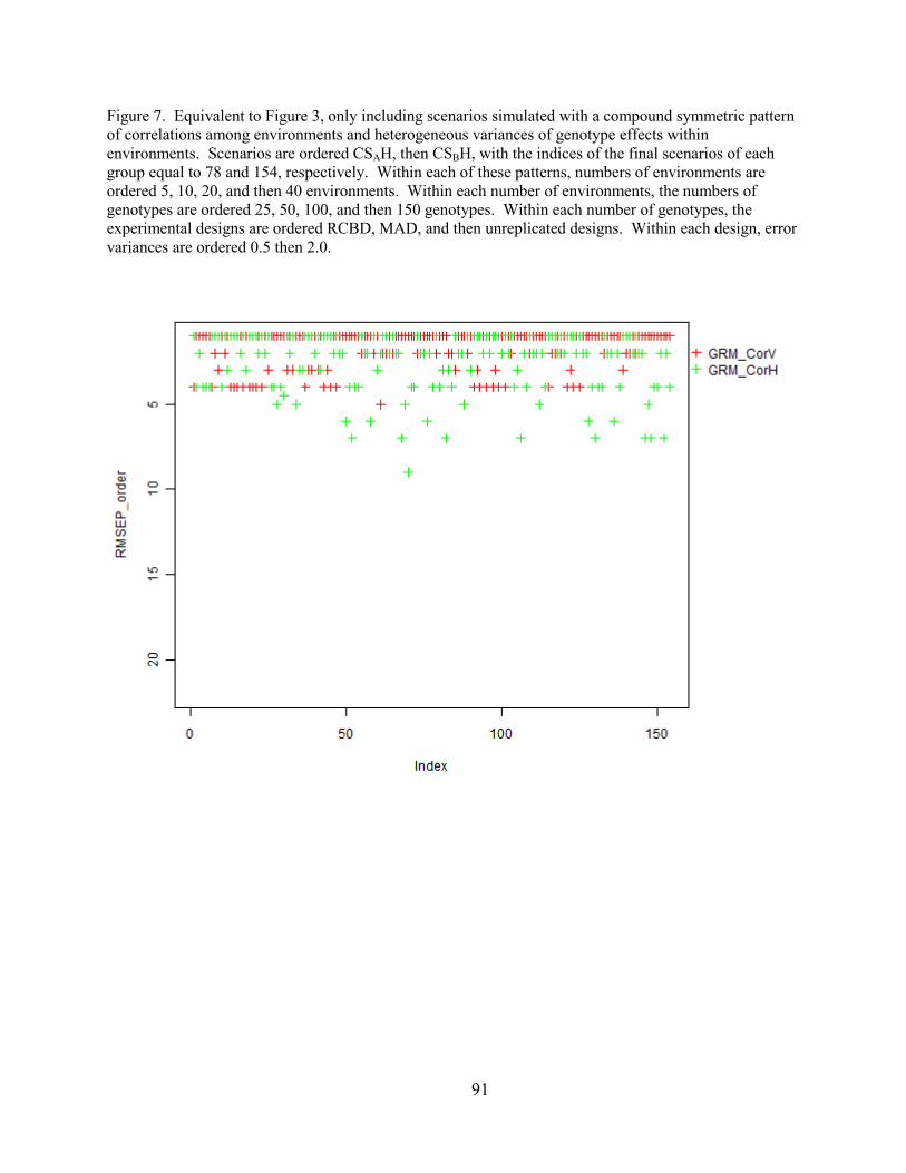
91
Figure 7. Equivalent to Figure 3, only including scenarios simulated with a compound symmetric pattern
of correlations among environments and heterogeneous variances of genotype effects within
environments. Scenarios are ordered CSAH, then CSBH, with the indices of the final scenarios of each
group equal to 78 and 154, respectively. Within each of these patterns, numbers of environments are
ordered 5, 10, 20, and then 40 environments. Within each number of environments, the numbers of
genotypes are ordered 25, 50, 100, and then 150 genotypes. Within each number of genotypes, the
experimental designs are ordered RCBD, MAD, and then unreplicated designs. Within each design, error
variances are ordered 0.5 then 2.0.

92
Figure 8. Equivalent to Figure 3, only including scenarios simulated with a compound symmetric pattern
of correlations among environments and extremely heterogeneous variances of genotype effects within
environments. Scenarios are ordered CSAVH, then CSBVH, with the indices of the final scenarios of each
group equal to 76 and 152, respectively. Within each of these patterns, numbers of environments are
ordered 5, 10, 20, and then 40 environments. Within each number of environments, the numbers of
genotypes are ordered 25, 50, 100, and then 150 genotypes. Within each number of genotypes, the
experimental designs are ordered RCBD, MAD, and then unreplicated designs. Within each design, error
variances are ordered 0.5 then 2.0.
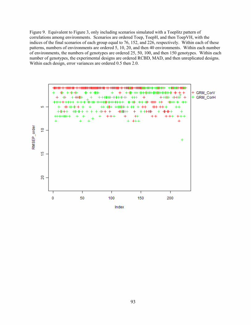
93
Figure 9. Equivalent to Figure 3, only including scenarios simulated with a Toeplitz pattern of
correlations among environments. Scenarios are ordered Toep, ToepH, and then ToepVH, with the
indices of the final scenarios of each group equal to 76, 152, and 226, respectively. Within each of these
patterns, numbers of environments are ordered 5, 10, 20, and then 40 environments. Within each number
of environments, the numbers of genotypes are ordered 25, 50, 100, and then 150 genotypes. Within each
number of genotypes, the experimental designs are ordered RCBD, MAD, and then unreplicated designs.
Within each design, error variances are ordered 0.5 then 2.0.

94
Figure 10. Equivalent to Figure 3, only including scenarios simulated with a Toeplitz pattern of
correlations among environments, 100 or 150 genotypes, 5 to 20 environments, and low (0.5) error
variance. Scenarios are ordered Toep, ToepH, and then ToepVH, with the indices of the final scenarios
of each group equal to 14, 29, and 43, respectively. Within each of these patterns, numbers of
environments are ordered 5, 10, and then 20 environments. Within each number of environments, the
numbers of genotypes are ordered 100 and then 150 genotypes. Within each number of genotypes, the
experimental designs are ordered RCBD, MAD, and then unreplicated designs.

95
Figure 11. Equivalent to Figure 3, only including scenarios simulated with 25 genotypes. Scenarios are
ordered CSA, CSAH, CSAVH, CSB, CSBH, CSBVH, Toep, ToepH, and then ToepVH, with the indices of
the final scenarios of each group equal to 24, 48, 72, 96, 120, 144, 168, 192, and 216, respectively.
Within each of these patterns, numbers of environments are ordered 5, 10, 20, and then 40 environments.
Within each number of environments, the experimental designs are ordered RCBD, MAD, and then
unreplicated designs. Within each design, error variances are ordered 0.5 then 2.0.
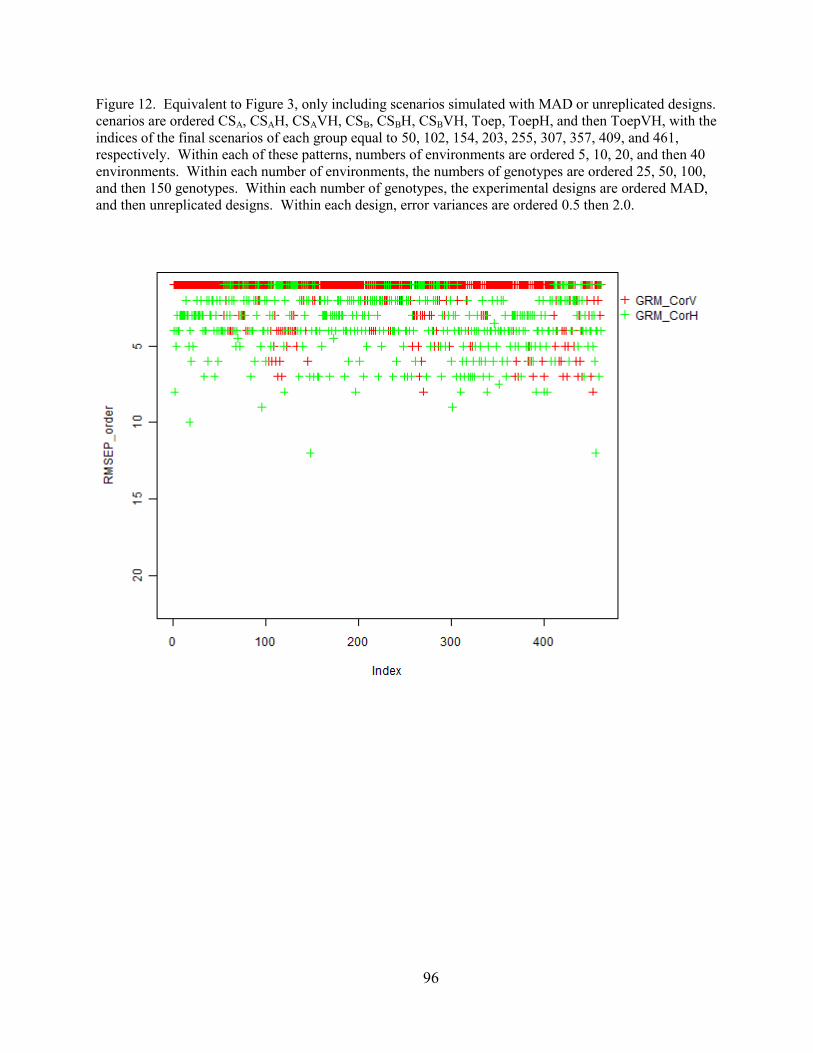
96
Figure 12. Equivalent to Figure 3, only including scenarios simulated with MAD or unreplicated designs.
cenarios are ordered CSA, CSAH, CSAVH, CSB, CSBH, CSBVH, Toep, ToepH, and then ToepVH, with the
indices of the final scenarios of each group equal to 50, 102, 154, 203, 255, 307, 357, 409, and 461,
respectively. Within each of these patterns, numbers of environments are ordered 5, 10, 20, and then 40
environments. Within each number of environments, the numbers of genotypes are ordered 25, 50, 100,
and then 150 genotypes. Within each number of genotypes, the experimental designs are ordered MAD,
and then unreplicated designs. Within each design, error variances are ordered 0.5 then 2.0.

97
Figure 13. A standardized version of Figure 1, where only models not including GRM have been ranked
within each scenario in terms of their mean ranks. The order of scenarios is the same.

98
CHAPTER 4
CONSULTING PROJECTS
As part of my Ph.D. I consulted on three projects where I provided statistical analysis of data
generated by other researchers. Below I introduce each project with an abstract or summary and
then describe the methods used along with reasons for and consequences of the methods. For the
Fusarium crown rot projects I began consulting after all the data had been collected and so had to
adapt my methods to suit the realities of the project. In the cold tolerance project I was able to
help devise methodologies which were then further modified based on the results of my analyses.
Heritability and Genetic Correlation Analyses for Fusarium
Crown Rot Resistance Assays of Wheat Mapping Population
Abstract
The following abstract is from: G.J. Poole, R.W. Smiley, T. C. Paulitz, C.A. Walker, A.H.
Carter, D.R. See and K. Garland-Campbell. 2012. Identification of quantitative trait loci (QTL)
for resistance to Fusarium crown rot (Fusarium pseudograminearum) in multiple assay
environments in the Pacific Northwestern US. Theoretical and Applied Genetics (In Press). It is
used here to summarize the project I collaborated on. My participation began after all data had
been collected and a preliminary analysis had been conducted.
Fusarium crown rot (FCR), caused by F. pseudograminearum and F. culmorum, reduces wheat
(Triticum aestivum L.) yields in the Pacific Northwest (PNW) of the U.S. by as much as 35%.
Resistance to FCR has not yet been discovered in currently grown PNW wheat cultivars. Several
significant quantitative trait loci (QTL) for FCR resistance have been documented on
chromosomes 1A, 1D, 2B, 3B, and 4B in resistant Australian cultivars. Our objective was to
identify QTL and tightly linked SSR markers for FCR resistance in the partially resistant
99
Australian spring wheat cultivar Sunco using PNW isolates of F. pseudograminerarum in
greenhouse and field based screening nurseries. A second objective was to compare heritabilities
of FCR resistance in multiple types of disease assaying environments (seedling, terrace, and
field) using multiple disease rating methods. Two recombinant inbred line (RIL) mapping
populations were derived from crosses between Sunco and PNW spring wheat cultivars Macon
and Otis. The Sunco/Macon population comprised 219 F6:F7 lines and the Sunco/Otis population
comprised 151 F5:F6 lines. Plants were inoculated with a single PNW F. pseudograminearum
isolate (006-13) in growth room (seedling), outdoor terrace (adult) and field (adult) assays
conducted from 2008 through 2010. Crown and lower stem tissue of seedling and adult plants
were rated for disease severity on several different scales, but mainly on a numeric scale from 0
to 10 where 0=no discoloration and 10=severe disease. Significant QTL were identified on
chromosomes 2B, 3B, 4B, 4D, and 7A with LOD scores ranging from 3 to 22. The most
significant and consistent QTL across screening experiments was located on chromosome 3BL,
inherited from the PNW cultivars Macon and Otis, with maximum LOD scores of 22 and 9
explaining 36% and 23% of the variation, respectively for the Sunco/Macon and Sunco/Otis
populations. The SSR markers Xgwm247 and Xgwm299 flank this QTL and are being validated
for use in marker assisted selection for FCR resistance. This is the first report of QTL associated
with FCR resistance in the U.S.
Discussion of Statistical Methods
Separate analyses were conducted for each mapping population, but methods and models were
consistent for the two populations. Experimental units for the growth room and outdoor terrace
bed screening experiments were individual plants within a cone-tainer. Experimental units for
the field screening experiments were individual plots, from which 5 individual stems were sub-

100
sampled and averaged. Averaging over subsamples has the benefit of reducing plot-to-plot
variation due to errors in FCR severity assessment, thereby aiding in identifying QTL and
increasing heritability.
The mapping populations were planted and tested in similar experimental designs for the
growth chamber and terrace screening experiments and a different design in the field. These
experiments were conducted prior to my involvement in the project. In all three screening
experiments, multiple assays were conducted at different time points and, for field screens only,
at different locations. In the greenhouse and terrace beds, the recombinant inbred lines (RIL)
from the mapping populations were divided into sets, each set including the same check
genotypes. These sets were planted in separate growth chambers or sections of the outdoor
terrace beds. A randomized complete block design was implemented within each growth
chamber or terrace bed section. These designs were used, because the desired number of
genotypes and replicates could not be fit in one growth chamber or terrace bed section. The field
experimental design did not divide the genotypes into sets and used a randomized complete
block design within each field. For the growth chamber and terrace experiments, the sets acted
as incomplete blocks, and so necessitated the assumption that there were no interactions between
the conditions of the set (growth camber or terrace bed) and the effects of genotypes (Dean and
Voss, 1998 p. 348). This assumption was also made for randomized complete block designs.
Additionally, effects of sets were assumed to be estimable using only the data from the checks.
These assumptions may not have been valid, especially for the terrace bed sections, since
growing conditions differed noticeably among the terrace bed sections, likely causing differences
in Fusarium infection pressure, to which the genotypes may have shown varying responses. In
some situations, incomplete blocks are unavoidable, due to restrictions on the number of

101
experimental units per block. However, in this study, either a randomized complete block design
or a general complete block design could have been used. Use of either design would have
provided more data, beyond the checks, to estimate growth room or terrace bed section effects.
Use of the general complete block design would have additionally allowed for the estimation of
growth room/terrace bed by genotype interactions (Dean and Voss, 1998 p. 313).
Variance components analyses were conducted separately for each screening experiment
using the SAS System software v9.2 (SAS Institute Inc., 2003) Mixed procedure. Analyzing the
data from all three screening experiments together would have necessitated a very complex
model, since the screening experiments would be expected to have heterogeneous variances and
correlated genotypic effects. The models used all shared the general form: Y = μ + Zγ + ϵ,
where Y is the vector of FCR severity scores, μ is the overall mean, γ is the vector of random
effects, Z is the associated incidence matrix, and ϵ is the vector of experimental errors. The
terms γ and ϵ are considered independent with variance-covariance matrices of G and R,
respectively. The variance-covariance matrices G differed between the screening experiments,
but in all cases all covariances were assumed equal to zero. This describes a standard random
effects model that allows estimation of heritability by estimating variance components for all
conditions known to vary among experimental units. For growth room and terrace data, variance
parameters were included for random effects of assay, sets within assays, replicates within sets
and assays, and genotypes within sets and assays. For field data, variance parameters were
included for assay, replicates within assays, and genotypes. Experimental error variance was
assumed constant ( ) for all observations and normally distributed. The assumption
of constant error variance, especially across assays within screening experiments, may not be
ideal. However, allowing for heterogeneity of error variances would have made heritability

102
estimates much less straightforward. These assumptions were checked, and in the case of the
field data from both populations, modest departure from the assumptions of both constant
variance and normality were detected. Therefore, some inaccuracy in the estimates of residual
variance, standard errors for the variance component estimates, and z-tests are expected (Kutner
et al., 2004 pp. 793–794). Assumptions were not substantially violated for the other data sets.
Broad-sense heritability (H2) on a genotype mean basis was estimated over all assays of
each screening experiment using the formula: H2 =
, where
is the estimated variance of
the genotypic effect and is the estimated variance of the phenotypic effect. Here, H
2 differs
from narrow-sense heritability (h2) only in terms of epistatic variance. Since the genotypes
evaluated here are RIL they are assumed to be fully homozygous. If the response unit is also an
inbred, then dominance has no influence on gain from selection. Therefore, H2 exceeds h
2 only
by the epistatic variance; the degree to which epistasis influences specific quantitative traits is
unknown, but may be substantial (Reif et al., 2009; Miedaner et al., 2011). The SAS code
provided by Holland et al. (2003), modified according to the experimental design of each
screening experiment, was used for these analyses. The heritabilities within each assay and
experiment were also calculated, prior to my participation in the project, but their utility may be
limited. Although such estimates can provide some suggestions of the consistency or variability
of genetic and phenotypic variances, the statistical accuracy of separate estimates of H2 for each
assay are likely lower due to a reduced data set compared to estimates over all assays.
Additionally, estimates within assays are less meaningful from a breeding perspective, since both
selection and response generally occur over a range of assays (e.g. selecting based on results
from multiple years of field testing for genotypes that will perform consistently well in multiple
years and locations).

103
Least squares means for genotypes were calculated within each of the assays and
screening experiments. These least squares means were calculated using fixed effects versions
of the above models in the SAS GLM procedure, prior to my participation. The statistical
signficance of differences in LSmeans between the parents were determined using t-tests. This
removed the main effects for blocks and sets as estimated by ordinary least squares estimation.
The LSmeans values for each assay of each genotype differ from the best linear unbiased
predictions that could have been extracted from a random effects model. These least squares
means were used in the QTL analyses and the analyses described below, since these analyses
were limited in terms of model complexity. The QTL analysis was limited by the composite
interval mapping models used by the QTL analysis software. Individual marker effects and
genetic correlations were analyzed on the same data so that the estimates could be compared to
the results of the QTL analysis.
The influence of assay-to-assay variation on marker effects was investigated using
separate analyses of variance for each combination of population, marker, and screening
experiment using the SAS Mixed procedure. Our analyses used the following model: Y = Xβ +
ϵ, where Y is the vector of FCR severity scores (lsmeans of each assay from the raw data
analysis), β is the vector of fixed effects of assay and marker allele, X is the associated
incidence/design matrix, and ϵ is the vector of experimental errors. Since assays were
considered repeated measures of each genotype (within marker allele), the covariance structure
for ϵ was modeled as compound symmetric for each genotype subject. The assumptions of this
method, that residuals are normally, independently, and identically distributed, were met for each
model within ranges that would not influence results. If significant interactions were detected
between marker and assay effects, each assay was tested for a significant marker effect

104
individually. This analysis acted as partial confirmation of the QTL analysis and suggested
which of the significant QTL had independent effects that could be discerned from background
noise. Although these evaluations are completely valid for these markers, these analyses don‟t
provide confirmation of the QTLs that is truly independent of the QTL analysis. These analyses
of variance used the same data as the QTL analysis and therefore suffered from the same
sampling biases. That is, if our observations of a marker in multiple assays happened to be
greater than the actual effect, the QTL analysis would flag the marker and we would have
concluded that there was a significant marker effect, consistent across assays. This is even more
likely than one might think, since markers that have a consistent effect across assays are more
likely to be significant QTLs and these analyses of variance were only conducted on highly
significant QTLs.
The genetic correlations between screening experiments and the genetic and phenotypic
variance specific to each was estimated with the SAS Mixed procedure using methods similar to
Holland (2006). Our analyses used the following model: Y = Xβ + Zγ + ϵ, where Y is the vector
of FCR severity scores (lsmeans of each assay from the raw data analysis), β is the vector of
fixed effects of assays within each screening experiment, X is the associated incidence/design
matrix, γ is the vector of random effects of genotypes in each screening experiment, Z is the
associated incidence matrix, and ϵ is the vector of experimental errors. The terms γ and ϵ are
considered independent with covariance matrices of G and R, respectively. We considered G
unstructured and identical for all genotypes, with separate variance parameters for each
screening experiment and heterogeneous covariances between each pair of screening experiment.
Experimental error variance (R) was modeled with heterogeneous variances across screening
experiments and no covariance between screening experiments. The assumptions of this method,

105
that residuals are normally, independently, and identically distributed, were tested and confirmed
for each model. Wald-type inference tests were used to test if genetic correlations differed from
zero.
By estimating genetic correlation with the above model using lsmeans of each assay from
the raw data analysis as the response, any effects of sets within assays, replicates within sets and
assays, or interactions between genotypes and replicates were accounted for, at least to the extent
that these were accurately estimated within the restrictions of the experimental design.
Therefore, the response variable should only be influenced by genotype, screening experiment,
assay within experiment, and their interactions, assuming that no latent variables have been
missed in the raw data analysis. Since we modeled the raw data with a model that included
terms for genotypes within experiments and fixed effects of assays within experiments, the
residual error associated with the genetic correlation should be equivalent to the genotype by
assay within experiment interaction (assuming no latent variables). Covariance between
screening experiments, and by extension phenotypic correlation between experiments, could not
be evaluated in this study because the same environmental conditions cannot be replicated in
different screening experiments, i.e. assays are nested within experiments.

106
Linear Modeling of the Relationships Between Wheat Field
Characteristics and Fusarium Crown Rot Observations
Abstract
The following Abstract is from: Grant J. Poole, Richard W. Smiley, Carl Walker, Kimberly
Garland-Campbell, Timothy C. Paulitz. A survey of Fusarium crown rot in dryland wheat in the
Pacific Northwest of the US. (Unpublished) It is used here to summarize the project I
collaborated on. My participation began after all data had been collected and a preliminary
analysis had been conducted.
Fusarium crown rot (FCR) is one of the most widespread root and crown diseases of wheat in the
Pacific Northwest of the U.S. Accurate surveys of pathogen and disease presence are needed to
determine the extent and damage due to FCR. Our objectives were to conduct a survey covering
the diverse dryland wheat-producing areas of Washington and Oregon, to determine the
geographic species distribution of causal agents of Fusarium crown rot, and to determine if
various environmental and geographical features of the collection location were associated with
species distribution. In this study 105 fields were surveyed during 2008 and 2009. Isolates of
Fusarium spp. were obtained from 99% of fields in 2008 and 97% of fields in 2009. Fusarium
culmorum was isolated from 31% of the symptomatic stems surveyed, closely followed by F.
pseudograminearum isolated at a frequency of 30% (symptomatic stems) averaged over both
survey years. Overall isolation frequency means for other minor species included F.
crookwellense, F. acuminatum, F. equiseti, and Bipolaris sorokiniana at 13%, 1%, 1%, and 2%,
respectively. Species composition and disease severity varied significantly depending on
geography and cropping system. F. pseudograminearum occurred in a greater frequency in
areas of the PNW with warmer and drier weather patterns, whereas F. culmorum occurred in
greater frequency from zones with moderate to high moisture and cooler temperatures.
107
Discussion of Statistical Methods
Statistical analyses were carried out to determine how field characteristics relate to Fusarium
culmorum and F. pseudograminearum infection. Factor analysis was used to estimate latent
factors from the highly correlated, continuous, field characteristic variables. The estimated latent
factors were used, with additional variables not included in the factor analysis, as predictor
variables in linear mixed models and generalized linear mixed models of the Fusarium infection
responses.
Data were collected from surveys, during 2008 and 2009, of 200 fields located in major
wheat growing regions of Washington and Oregon. In 2008, 100 fields were surveyed, and in
2009, a matched field, no more than 3.2 km away was surveyed, since wheat was not grown on
each field each year. These matched pairs were considered to have the same values for every
explanatory variable.
Climate data used in this analysis were 30 year averages and were retrieved from the US
Forest Service Rocky Mountain Research Station website
(http://forest.moscowfsl.wsu.edu/climate/current/) for each specific GPS point survey location.
These data are potentially useful for predicting FCR infection, since a given year‟s weather
conditions are partially predicted by average conditions. However, year to year climatic
variation is always large. Some of this variation was captured as overall year effects in linear
models, but some of the variation was not attributable to year main effects or 30 year averages.
Therefore, estimates using these data would be expected to be less accurate than if actual weather
data were recorded. Unfortunately, resources were limited, necessitating the use of data that are
freely available.

108
Soil textures were categorized as one of three classification categories: sandy loam, loam,
or silty loam. Although the categories cover a range of values, we chose the center point of each
category and assigned all observations of that category sand, silt, and clay contents equal to the
center values. Doing so resulted in some loss of information, since the categories encompass
more possibilities than captured by the center points. For the centers of these three categories,
the amounts of sand and silt are almost perfectly negatively correlated and the amount of clay
doesn‟t vary to a meaningful degree. Therefore, we chose the percent sand content as a
replacement variable for the original categorical soil texture variable. Using all three continuous
variables would result in extreme multicollinearity, which should be avoided in linear modeling.
The benefits of using sand content instead of texture classes were that it allowed a single variable
to replace two indicator variables, it correctly placed loam soils intermediate to sandy loam and
silty loam soils, and since it was a continuous variable, it could be easily incorporated into
dimension reduction techniques.
The field characteristic „percent cropped‟ indicates the estimated percentage of time and
area that a crop was grown on a field. These values were estimated based on data from National
Agricultural Statistics Service analysis of satellite images. The estimated values are from the 12
km area centered on each field, during the growing season, over multiple years. These data
provide information as to how much time the field spent in fallow prior to sampling of the wheat
crop. Unfortunately, the limited resolution of 12 km around the field means that other fields and
non-cropped lands may have been captured in the estimate. Despite such limitations on
accuracy, these data were considered superior to other options for estimating cropping system
with limited resources.

109
Prior to factor analysis, correlations were calculated to estimate relatedness among
continuous field characteristic variables. Pearson correlations were calculated between
elevation, mean annual temperature, mean annual precipitation, mean temperature in the coldest
month, mean temperature in the warmest month, percent cropped, and soil sand content. Only
variables which had correlation coefficients of greater than 0.5 with at least one other variable
were included in the factor analysis, so sand content was not included. This correlation analysis
provided some indication as to whether multicollinearity was present in the explanatory
variables. High correlation values indicate definite multicollinearity, but multicollinearity could
also occur between sets of more than two variables even if all pairwise correlations were low.
However, in this situation, with only seven explanatory variables, there was limited potential for
high levels of multiple variable dependency without pairwise correlation.
Factor analysis was conducted using the FACTOR and SCORE procedures with the
common factor method in SAS (SAS Institute Inc., 2003) to estimate latent factor values for each
field for two rotated factors. Factor analysis was chosen for dimension reduction over principal
components analysis, because the field characteristic variables used in this analysis were
considered imprecise measurements of the true variation across these fields. Principal
component analysis does not have this same philosophical underpinning (Suhr, 2005).
Underlying latent variables were assumed, since weather patterns, which varied over the wide
geographic region sampled, influenced all the climate traits and growers‟ cropping systems
decisions. Analysis was limited to two factors based on the scree test and the Kaiser-Guttman
rule. The initial factor solution was rotated to improve interpretation using a varimax rotation.
This rotation was chosen because it yields orthogonal latent factors, and the primary goal of our
factor analysis was to avoid multicollinearity in the linear modeling that followed.

110
Repeated measures analyses were conducted to relate the field characteristics to the
response variables (FCR severity scores and node infection scores). The two response variables
were analyzed similarly using the MIXED procedure in SAS (SAS Institute Inc., 2003) and a
model which included the two estimated latent factors, sand content, and year as fixed effects
including all two-way interactions. Each pair of matched fields was considered the subject of
repeated measures. That is, the assessment of one field in 2008 and its matched field in 2009 are
considered repeated measures on the same subject. Linear mixed model assumptions were
checked and met for both response variables. When significant interactions were observed,
simple effects of each level of one variable were tested and estimated at each level of the other.
The use of repeated measures analysis and the consideration of matched fields to be observations
on the same subject was the most appropriate analysis on a non-ideal design. Ideally, the same
field would have been observed both years, but crop rotation made this impossible for most of
the fields. Alternatively, a different set of fields could have been evaluated each year, although
this would necessitate sufficient numbers of fields to ensure that the same sample space of the
predictor variables was covered in both years. Due to limitations in funds and time, evaluation
of more than 100 fields per year was not possible, so this match-fields design was an effective
compromise.
Presence or absence of F. culmorum and F. pseudograminearum on five stems from each
field was related to field characteristics and year effects using the GLMMIX procedure in SAS
(SAS Institute Inc., 2003). If the underlying field conditions result in a certain probability that
each stem will get infected with a given species, then testing five independent stems is a
binomial response. Therefore, a generalized linear model with a logit link was appropriate.
With these separate analyses for each species, we made the assumption that presence of one

111
species does not affect the presence of the other. This assumption was partially justified by our
observations of the presence of both species on some stems. Allowing for influence between
species would have required a more complex model that would likely be beyond the information
content of the data. A generalized linear mixed model of repeated measures was fit using a logit
link. Each pair of matched fields was considered the subject of repeated measures. As described
above, other designs might have been preferable, given greater resources. Reported effects and
95% confidence intervals were estimated using models which only included those terms
identified as significant in the full model.

112
Logistic Regression Analysis of Wheat Cold Tolerance
Testing
My participation in this project began prior to the testing and analysis described below, and as
such I contributed to the choices of methods and experimental design.
Summary
The ability of both winter and spring genotypes to survive extreme cold has economic
repercussions in Washington and thus is an important target for wheat breeders. The genetics
that underpin tolerance to extreme cold have not been fully elucidated, so breeders must rely on
phenotypic evaluations. Assessment of cold tolerance in the field is impaired by variations
across years and within a field, necessitating testing under controlled conditions. The objective
of this study was to develop and implement a set of procedures and analyses to evaluate
genotypes for tolerance to extreme cold within a breeding program. Wheat was grown within
cells of soil and was subjected to extreme cold that had a differential effect on survival.
Temperature recording probes in each cell were used to measure the temperature variation
among cells of soil every 2 minutes during a freeze test procedure. A calibration based on
temperature readings of freezing water was used in an attempt to adjust for inaccuracies in the
probe readings. Logistic regression was performed to compare survival of test genotypes to the
check cultivars, resulting in estimates of odds ratios and corresponding confidence intervals.
These confidence intervals let us identify which genotypes were significantly worse, better, or
not significantly different from the controls, and this allows for ranking of test genotypes while
statistically accounting for error in estimation. Accuracy using calibrated and un-calibrated
probe data and using survival data alone was evaluated by taking the Spearman correlation
between odds ratios calculated on the 2010 freeze trials of winter genotypes and the estimates

113
derived from the 2011 freeze trials. The correlations were: 0.493, 0.460, and 0.443, for no probe
data, probe data, and calibrated probe data, respectively. These results suggest that, at least when
only one minimum temperature is used, use of probe data, with or without calibration does not
improve the accuracy of tolerance estimation.
Discussion of Methods
Multiple sets of winter and spring wheat germplasm were evaluated for tolerance to extreme cold
temperatures in 2009, 2010, and 2011. These sets included released cultivars, breeding material,
and mapping populations. Sets of test genotypes that could be considered from the same
population were analyzed together. Division into populations was partially subjective, but was
based on expectations of cold tolerance for a population. Separation based on growth habit is
obviously necessary, since no single temperature will allow both winter and spring genotypes to
show differential survival, i.e. too cold a temperature will kill all the spring cultivars and vice
versa. Released cultivars and breeding material were separated from mapping populations, since
the mapping populations derive from a single cross. Progeny from a single cross should have
reduced variability, as compared to less closely related cultivars and breeding material, and so
may have a different ideal test temperature. Two check genotypes were included with each set
of test genotypes. The cultivars Eltan, which has desirable cold tolerance, and Stephens, which
has insufficient cold tolerance, were used as checks with the winter genotypes. The cultivars
Alpowa, with good cold tolerance (for a spring growth habit genotype), and Zak, with poor cold
tolerance, were used as controls for the spring genotypes. Different checks for winter and spring
populations were necessary not only to match the vernalization requirements of the test

114
genotypes, but also because checks are only useful if they fit within the distribution of the test
genotypes.
Prior to cold tolerance testing, the test and check genotypes were grown in conditions
mimicking fall growing conditions. The wheat seeds were densely planted in small cells of soil,
twenty seeds per cell. The plants were grown in warm conditions 22°C day/15°C night for one
week, followed by five weeks at 4°C. Immediately prior to testing, the number of seedlings that
had grown in each cell was recorded and cells were watered to saturation with a 10 mg/L
solution of SNOWMAX® (Johnson Controls, Centennial, CO, USA). Snowmax was added to
help reduce supercooling, thereby reducing chance variability among soil cell conditions.
However, Snowmax was probably not necessary after the sub-zero acclimation period (described
below) was adopted in 2010, since this allowed cells to all freeze at a non-lethal temperature
prior to imposition of extreme cold, and the freezing temperature of water in soil is 0°C (Lackner
et al., 2005).
Testing for extreme cold tolerance was conducted in a programmable freezer (model LU-
113, Espec Corp., Hudsonville, MI, USA) using three temperature profiles, one for winter
genotypes and two profiles for spring genotypes. Runs of 48 soil cells were placed in the freezer
at the same time. It is important to note that the freezer settings did not necessarily match the
actual temperatures of the air inside the chamber or the soil in each cell. The temperature of
each cell of soil was recorded at 2 minute intervals using food piercing temperature probes
connected to a monitor system that connected to multiple personal computers. The temperature
profiles used were similar to those of Skinner and Bellinger (2011). All temperature profiles
began by cooling the freezer and holding at a setting of -3°C for 16 hours for tests in 2010 and
2011. This will be referred to as the sub-zero acclimation period (SZAP). Tests in 2009 did not

115
include a SZAP and began the same temperature profile from room temperature. Skinner and
Bellinger (2010) observed that a 16-hour SZAP increased cold tolerance in winter wheat. This
was not our goal for the SZAP, since growing conditions in the field may not necessarily be as
gradual. The SZAP was instead included because it ensures that all soil cells are frozen by the
time colder temperatures are imposed. Omitting a SZAP period results in dramatic variability in
the temperatures that occur in each soil cell. The soil cells vary in terms of water holding
capacity, due to differences in actual mass of soil contained and packing density, and latent heat
from the freezing process prevents the soil cells from cooling further while the phase change
occurs. This means that without a SZAP some soil cells will still be freezing while others are
decreasing in temperature post-freezing. Following the SZAP, the winter genotypes were cooled
for 2.5 hours to a temperature setting of -13°C, which was held for 1 hour. Temperatures were
then increased to 4°C over a period of 4.25 hours. The warmer profile for spring genotypes
consisted of cooling after the SZAP for 0.75 hours to -6°C, holding at -6°C for 1 hour, then
warming for 2.5 hours. The cooler spring profile was cooling for 1.25 hours to -8°C, holding at -
8°C for 1 hour, then warming for 3 hours. The minimum temperatures used were selected to
result in the greatest range of probabilities of survival and to result in differential survival
between the check genotypes. Using too cold or too warm a minimum will result in many
genotypes with no or complete survival, preventing differential survival. Winter genotypes were
tested at a single temperature as a matter of efficiency. In breeding program evaluations for
selection, high-throughput procedures with modest accuracy are preferred to precisely estimating
small differences among genotypes. Multiple temperatures were used for spring genotypes in the
process of identifying the ideal temperature for each set of genotypes, and data were analyzed
separately for each minimum. Following the extreme cold treatment, seedling leaves were cut

116
off at the soil line. After one day at 4°C, the seedlings were grown in a greenhouse for five
weeks, and the plants that regrew were recorded as having survived.
In response to observed variability in probe readings for known temperatures, a
calibration of output temperature values was attempted. Obviously malfunctioning probes were
replaced beforehand, but minor inaccuracies could not be easily identified prior to calibration.
The probes were all placed in the same container of distilled water within the freezer, which was
lowered and held below freezing. The volume of water was sufficient that the period of phase
change from liquid to ice lasted long enough to appear as a horizontal line of constant
temperature in the probe data readings. Since the phase change of distilled water occurs at 0°C,
the deviation of each probe from 0°C during the phase change was considered error. This
estimated error value for each probe was subtracted from all of that probe‟s reported values to
calibrate the probe output. This method of calibration is obviously not ideal. Although it could
be expected to effectively determine the degree of error for each probe at 0°C, the error at the
more important and damaging temperatures may differ, possibly resulting in over- or under-
adjustment. It is also possible that probe errors are not constant over time. If the deviation
changed signs, the calibration adjustment would in fact be opposite the correct direction at the
time of the test. In light of these shortcomings, the effectiveness of calibration was compared to
not adjusting the raw probe data.
Probe temperature output data, with and without calibration, were used to calculate
metrics that described components of the temperature profiles of each extreme cold treatment.
These calculations were similar to those of Skinner and Mackay (2009) and Skinner and
Bellinger (2011). These profile components were used, since Skinner and Mackay observed that
survival in some populations was related to metrics other than just minimum temperature.

117
Temperature differences above -5°C were considered unimportant, since the temperature of the
SZAP (-3°C setting on the freeze chamber) is uniformly tolerable for all the genotypes tested and
temperatures recorded by the probes during the SZAP are sometimes lower than -3°C. The post-
SZAP was defined as the period between the first time each probe recorded a temperature of -
5°C and the next time the probe recorded -4.6°C. The higher ending temperature ensures that
small fluctuations in temperature do not result in the incorrect identification of very short post-
SZAP. For each post-SZAP, multiple components of the temperature profile were calculated.
The post-SZAP duration and minimum temperature are self-explanatory. The post-SZAP was
parsed into three periods: the cooling period, the at-minimum period, and the warming period.
The at-minimum period was defined as the time during which temperatures were within 0.5°C of
the minimum temperature. This ensures that minor temperature fluctuations around the
minimum are ignored. The cooling and warming periods preceded and followed the at-minimum
period, respectively. The duration of each of these periods was calculated. The cooling and
warming rates were defined as the change in temperature during each period divided by the
duration of each respective period. Degree minutes were calculated as:
F
i
iiii
TTtt
1
1)1(
2,
where ti is the ith
time point, Ti is the temperature at the ith
time point, and F is the number of
time points recorded during the post-SZAP.
Logistic regression was performed using the LOGISTIC procedure of the SAS/STAT
software (SAS Institute Inc., 2003) to compare survival of test genotypes to the check cultivars
using survival data with both calibrated and un-calibrated probe data and using survival data
alone. Logistic regression is valid when each plant is considered an experimental unit and
survival or death of each plant is the binary response. It is appropriate to think of individual
118
plants as experimental units, because survival was assessed for each plant individually and each
plant responds independently to the soil and temperature conditions specific to each cell of soil.
The conditions of each soil cell were included in the analysis via the temperature profile
components used as covariates in the logistic regression. When analyses were conducted without
probe data, cell-to-cell variation was no longer captured in the model. Therefore, without probe
data, the assumption of independent error for each plant may have been violated. The expected
cell-to-cell variation could have been included in the model with the use of a generalized linear
mixed model. Unfortunately, such models often failed to converge when applied to the large
data sets in this study. Smaller subsets of genotypes could have been separately analyzed, but
that would have produced different statistical conclusions (inference tests, confidence intervals,
etc.) depending upon which genotypes were analyzed together.
The genotype factor and the seven temperature profile components define a set of 255
possible first order models without interactions. Specific models varied among data sets and
were chosen using stepwise regression in the LOGISTIC procedure with entry and exit
significance levels of 0.05. Test genotypes were evaluated by generating confidence intervals of
the ratios of odds of survival of each test genotype against each control genotype. These
confidence intervals let us identify which genotypes were significantly worse, better, or not
significantly different from the controls. Using two checks for comparisons allows test
genotypes to be separated into five groups: worse than the inferior check, equivalent to the
inferior check, in between the two checks, equivalent to the superior check, or better than the
superior check. This grouping allows for ranking of test genotypes while statistically accounting
for error in estimation. Rankings based on estimated odds ratios or percent survival do not

119
reflect the sampling errors that may cause inaccurate rankings among similarly performing
genotypes.
Accuracy using calibrated and un-calibrated probe data and using survival data alone was
evaluated by taking the Spearman correlation between the odds ratios (with Eltan or Stephens as
reference) calculated on the 2010 freeze trials of winter genotypes and the estimates derived
from the 2011 freeze trials. Spearman correlations were used to minimize the effect of outliers,
since odds ratio estimates vary more drastically at the extremes. This analysis included only
genotypes that were tested in both years and, in 2011, were tested after malfunctioning probes
were replaced on 3/23/11. This resulted in 45 genotypes used in the comparisons. The
Spearman correlations, with Eltan as the reference for the odds ratios, were: 0.493, 0.460, and
0.443, for no probe data, probe data, and calibrated probe data, respectively. The correlations
using Stephens as the reference genotype were very similar and showed the same pattern. This
comparison indicated that the use of probe data, with or without calibration, does not improve
predictive ability. The futility of the calibration was not unexpected, due to the limitations
described above. However, the use of probe data was expected to improve predictions based on
the results of Skinner and Mackey (2009), who observed that temperature probes could record
changes in conditions that influenced survival. The difference in conclusions may be explained
by the differences in the temperature profiles used in each study. Skinner and Mackey lowered
temperatures to two different minimums, as opposed to the single minimum we used for the
winter genotypes, and did not include a SZAP. Their methods resulted in a much larger range of
conditions. When a SZAP was included with only a single minimum in our study, temperature
variation among cells was much less. This variation was likely within the margin of error for the
temperature probes, making their output useless for predicting survival.

120
The correlation of 0.493, between 2010 and 2011 results based on survival data alone,
indicates that substantial variation in survival is unaccounted for by genotype. This additional
variation may be attributable to cell-to-cell temperature variability that was not successfully
captured by the probe data or variation in growing and testing conditions between 2010 and
2011. Additional replication of cells and/or testing over time will be necessary to provide
accurate and precise estimates of extreme cold tolerance, but evaluation within a single year
should be sufficient for coarse selection decisions.
References
Dean, A.M., and D. Voss. 1998. Design and Analysis of Experiments. Springer.
Holland, J.B. 2006. Estimating Genotypic Correlations and Their Standard Errors Using
Multivariate Restricted Maximum Likelihood Estimation with SAS Proc MIXED. Crop
Science. 46(2): 642–654.
Holland, J.B., W.E. Nyquist, and C.T. Cervantes-Martínez. 2003. Estimating and Interpreting
Heritability for Plant Breeding: An Update. : 9–112.
Kutner, M., C. Nachtsheim, J. Neter, and W. Li. 2004. Applied Linear Statistical Models. 5th ed.
McGraw-Hill/Irwin, San Francisco.
Lackner, R., A. Amon, and H. Lagger. 2005. Artificial Ground Freezing of Fully Saturated Soil:
Thermal Problem. Journal of Engineering Mechanics. 131(2): 211–220.
Miedaner, T., T. Würschum, H.P. Maurer, V. Korzun, E. Ebmeyer, and J.C. Reif. 2011.
Association mapping for Fusarium head blight resistance in European soft winter wheat.
Molecular Breeding. 28(4): 647–655.
Reif, J.C., B. Kusterer, H.-P. Piepho, R.C. Meyer, T. Altmann, C.C. Schön, and A.E.
Melchinger. 2009. Unraveling Epistasis With Triple Testcross Progenies of Near-
Isogenic Lines. Genetics. 181(1): 247 –257Available at (verified 20 January 2012).
SAS Institute Inc. 2003. SAS/STAT® User‟s Guide, Version 9. SAS Institute Inc., Cary, NC.
Skinner, D.Z., and B.S. Bellinger. 2010. Exposure to subfreezing temperature and a freeze-thaw
cycle affect freezing tolerance of winter wheat in saturated soil. Plant and Soil. 332: 289–
297.

121
Skinner, D.Z., and B.S. Bellinger. 2011. Differential Response of Wheat Cultivars to
Components of the Freezing Process in Saturated Soil. Crop Science. 51(1): 69.
Skinner, D.Z., and B. Mackey. 2009. Freezing tolerance of winter wheat plants frozen in
saturated soil. Field Crops Research. 113(3): 335–341.
Suhr, D. 2005. Principal Component Analysis vs. Exploratory Factor Analysis. In Proceedings of
the Thirtieth Annual SAS Users Group International Conference. SAS Institute Inc.,
Cary, NC.