Statistical Analysis of Gene Expression Microarray Data
128
Statistical Analysis of Gene Expression Microarray Data Lisa M. McShane Eric C. Polley Biometric Research Branch National Cancer Institute CIT, May, 2011 1 / 128
-
Upload
khangminh22 -
Category
Documents
-
view
4 -
download
0
Transcript of Statistical Analysis of Gene Expression Microarray Data

Statistical Analysis of GeneExpression Microarray Data
Lisa M. McShane Eric C. Polley
Biometric Research BranchNational Cancer Institute
CIT, May, 2011
1 / 128

CLASS OVERVIEW
Day 1 Discussion of statistical analysis of microarray data –Lisa McShane and Eric Polley
Day 2 Hands-on BRB ArrayTools workshop – SupriyaMenezes
2 / 128

OUTLINE
1 Introduction: Technology
2 Data Quality & Image Processing
3 Normalization & Filtering
4 Study Objectives
5 Design Considerations
3 / 128

1 Introduction: Technology
2 Data Quality & Image Processing
3 Normalization & Filtering
4 Study Objectives
5 Design Considerations
4 / 128

GENE EXPRESSION MICROARRAYS
Permit simultaneous evaluation of expression levels ofthousands of genes
Main Platforms:• Spotted cDNA arrays (2-color)• Affymetrix GeneChip (1-color)• Spotted Oligo arrays (1- or 2-color)• Bead arrays (e.g. Illumina-DASL)
5 / 128

SPOTTED CDNA ARRAYS
cDNA arrays: Schena et al., Science, 1995.
Each spot corresponds to a gene. Sometimes multiplespots per gene.
Two-color (two-channel) system:• Two colors represent the two samples competitively
hybridized• Each spot has “red” and “green” measurements
associated with it.
6 / 128

CDNA ARRAY
8 / 128

Figure: Overlaid “red” and “green” images for cDNA microarray9 / 128

AFFYMETRIX GENECHIP
Lockhart et al., Nature Biotechnology, 1996.
Affymetrix: http://www.affymetrix.com
Glass wafer (“chip”) — photolithography, oligonucleotidessynthesized on chip
Single sample hybridized to each array
Each gene represented by one or more probe sets:• One probe type per array “cell”• Typical oligo probe is 25 nucleotides in length• 11-20 PM:MM pairs per probe set (PM = perfect
match, MM = mismatch)
10 / 128

GENECHIP
Figure: Affymetrix Oligo “GeneChip” array 1
1http://en.wikipedia.org/wiki/DNA_microarray11 / 128

GENECHIP
Figure: Image of scanned Affymetrix GeneChip
12 / 128

GENECHIP
probes). RNA samples are prepared accordingto the protocol defined by Lockhart [1996], andthen the labeled RNA sample is hybridized tothe corresponding probes on the array. Thearray then goes through an automatedstaining/washing process using the Affymetrixfluidics station, and upon completion of thisprocess, the array is scanned using the Af-fymetrix confocal laser scanner. The scannergenerates an image of the array by excitingeach feature with its laser, detecting the re-sulting photon emissions from the fluores-cently labeled RNA that has hybridized to theprobes in the feature, and converting the de-tected photon emissions into a 16-bit intensityvalue. The images generated by the scannerare then ready for analysis. We can determinewhether a gene is present and the quantity atwhich it is present by examining various sta-tistics formed from the PM/MM feature inten-sities. Most of the statistics used are based onPM/MM differences (e.g., the average differ-ence intensity and the positive fraction andpositive/negative fraction statistics describedlater) and the PM/MM ratio (e.g., the averagelog-ratio). When a gene transcript is actuallypresent, one would expect the PM intensities tobe significantly greater than the MM intensi-ties, which would be reflected in the PM/MMdifferences, ratios and associated statistics.
The GeneChip software supplied by Af-fymetrix to process array images from thescanner performs all of the fundamental oper-ations necessary to analyze an array, including(1) image segmentation, (2) background correc-tion, (3) scaling/normalizing arrays for array-to-array comparisons, (4) calculation of statis-tics to indicate whether a gene transcript ispresent, and (5) calculation of statistics to in-dicate whether a gene transcript is differen-tially expressed. As will be detailed by Schadtet al. [1999], we have developed and imple-mented our own algorithms for each of theoperations listed above. We will discuss manyof these methods in a less technical mannerthroughout the remainder of this article. For amore detailed description of these methods andfor a more exhaustive comparison of thesemethods with currently available ones, refer toSchadt et al. [1999].
Computing Reliable Feature Intensities
Image Segmentation. In analyzing geneexpression array data generated by the Af-fymetrix GeneChip! technology, perhaps thesimplest operation to perform is that of seg-menting the image. The GeneChip softwareemploys a dynamic gridding algorithm to seg-ment the image and then uses a percentilealgorithm to compute the feature intensitiesonce the feature boundaries have been deter-mined [Lockhart et al., 1996]. We describe, inSchadt et al. [1999], our own image-processingalgorithm. Employing our own image segmen-tation algorithm allowed us to directly analyzethe distribution of pixel intensities for a givenfeature, devise new algorithms to compute fea-ture intensities, and directly estimate the blur-ring effects that can affect probe intensity cal-culations. The image files generated by theAffymetrix GeneChip! scanner are 16-bit, bi-nary image files, with header information pre-pended as described in the GATC specification[GATC Consortium, 1998]. Except for anoma-lous examples (e.g., when the laser in the Af-fymetrix GeneChip! scanner is not properlyaligned or when the image is extremely bright),we have found it straightforward to computerobust feature intensity estimates for a probearray. Aligning the basic grid to an image todetermine the feature locations is greatly sim-plified because the arrays contain alignmentfeatures at each corner of the image (thesefeatures can be seen in Fig. 1), which, when
Fig. 2. Hypothetical arrangement of oligonucleotides selected
to interrogate a single gene transcript (top). The perfect match
(PM) and mismatch (MM) probes designed to correspond to a
gene are synthesized in adjacent features (middle of figure). The
intensity plot represents the sort of hybridization intensities we
see for genes that are present at a moderately high abundance
(bottom). Note the functional dependency of the MM intensity
on the PM intensity; further note that, as expected, this func-
tional dependency is not linear with respect to PM intensity.
194 Schadt et al.
Figure: Perfect Matching - Mismatch Probe Pair2
2From Schadt et al., Journal of Cellular Biochemistry, 200113 / 128

1 Introduction: Technology
2 Data Quality & Image Processing
3 Normalization & Filtering
4 Study Objectives
5 Design Considerations
14 / 128

SPOTTED ARRAYS: QC
Figure: Background haze
Figure: Edge effect
Figure: Bubble Figure: Scratchor Fiber
• Visual inspection ofarrays advisable
• Danger:Garbage In⇒Garbage Out
15 / 128

GENECHIP: QC
duce the signal variation within and betweenarrays. Furthermore, a portion of the arrays wehave analyzed had noticeable signal anoma-lies, which included intensity gradients (brightedges and fluorescing streaks), glue smears(broad fluorescing strokes resulting from thechip packaging process), and dark spots (re-gions where the signal is artificially low). Fig-ure 1 illustrates some of these problems. Wehave found that the normalization and back-ground correction methods currently availableto analyze probe array data can be enhanced tobetter account for such problems, and thatmany of the underlying assumptions on whichthese methods depend do not hold in a signifi-cant percentage of the experiments we haveanalyzed. Finally, we have found it useful tosupplement the gene detection and differentialexpression detection methods employed by theGeneChip software with our own methods, tomake these results easier to interpret at thebiological level and to provide a more quanti-tative measure of significance on whether agene is present or differentially expressed.
We will discuss in more general terms someof the methods and tools we have developed tofacilitate the analysis of GeneChip data; meth-ods aimed at reducing variation at a variety of
sources, variation that serves only to obscurethe very biological variation we are actuallyinterested in detecting. We will begin with abrief overview of the oligonucleotide expressionarray technology developed by Affymetrix, andthen proceed to describe each of the low-levelanalysis methods we have found useful in an-alyzing gene expression array data.
OVERVIEW OF THE OLIGONUCLEOTIDEEXPRESSION ARRAY TECHNOLOGY
There are several publications discussing thefundamentals of the oligonuceotide expressionarray technology [see, e.g., Lockhart, 1996, orthe supplement to Nature Genetics, Volume21, January, 1999]. However, for our purposesin this article, it will be useful to review some ofthe elements of the probe array analysis pro-vided by the GeneChip! software. As describedby Lockhart et al. [1996], genes are repre-sented on a probe array by some number ofsequences (typically 20) of a particular length(typically 25 nucleotides) that uniquely iden-tify the genes and, ostensibly, have relativelyuniform hybridization characteristics, with re-spect to the experimental protocol used inthese experiments. Each oligonucleotide, orprobe, is synthesized in a small region (thelength and width of the features are either 50 !mfor the low-density arrays or 24 !m for thehigh-density arrays), which can contain any-where from 106 to 107 copies of a given probe.Designed to correspond to the perfect match(PM) oligonucleotide pulled from a gene se-quence (or EST), is a mismatch (MM) oligonu-cleotide in which, typically, the center baseposition of the oligo has been mutated; the MMprobes give some estimate of the random hy-bridization and cross hybridization signals, al-though, as we can see in Figure 2, there is anonlinear functional relationship between thepaired PM and MM probe intensities.
Ostensibly, this functional relationshipstems from the hybridization kinetics of thedifferent probe sequences and from nonspecificRNA hybridizations. Figure 2 illustrates a hy-pothetical tiling pattern of probes pulled from agene sequence, the length of the probes, andhow each PM probe is paired with a corre-sponding MM probe, and the intensity differ-ential between PM and MM features when agene is present in a sample (i.e., high intensityfor the designed perfect match probes, low in-tensity for the corresponding mismatch
Fig. 1. A contaminated D array from the Murine 6500 Af-fymetrix GeneChip" set. Several particles are highlighted byarrows and are thought to be torn pieces of the chip cartridgeseptum, potentially resulting from repeatedly pipetting the tar-get into the array.
193Analyzing Gene Expression Array Data
Figure: Affymetrix Arrays: Quality Problems3
3From Schadt et al., Journal of Cellular Biochemistry, 200116 / 128

SEGMENTATION
cDNA/2-color spotted arrays need to be segmented toextract data.
Segmentation: Separation of feature (F ) from background(B) for each spot.
Summary measures computed for F (for eachchannel/color):• Intensity: Mean or Median over pixels• Additionally: SD, Size (# pixels), etc.
17 / 128

SIGNAL CALCULATION
cDNA/2-color spotted arrays: Background correction &signal calculation (for each channel/color):• No background correction:
Signal = F
• Local background correction:Signal = F −Blocal
• Regional background correction:Signal = F −Bregion
18 / 128

FLAGGING SPOTS
cDNA/2-color spotted arrays: flagging spots/arraysexclusion
Exclude spots if “signal” or “signal-to-noise” measure(s)poor (low):• F• F −B• (F −B)/SD(B)
• Spot size
Exclude whole arrays or regions if:• Too many spots flagged• Narrow range of intensities• Uniformly low signals
19 / 128

2-COLOR ARRAYS: GENE-LEVEL SUMMARY
• Model-based methods:• Work directly on signals from two channels• Color effects and interactions between color and
experimental factors incorporated into statisticalmodels
• Ratio Methods†4
• Red signal / Green signal• “Green” sample serves as internal reference
4†Today’s course will focus on ratio methods20 / 128

AFFYMETRIX ARRAYS: IMAGE PROCESSING
• DAT image files→ CEL files• Each probe cell is 10× 10 pixels• Grid alignment to probe cells• Signals:
• Remove outer 36 pixels→ 8× 8 pixels• The probe cell signal, PM or MM, is the 75th
percentile of the 8× 8 pixel values
• Background correction: Average of the lowest 2%probe cell values in zone is taken as the backgroundvalue and subtracted
• Summarize over probe pairs to get gene expressionindices
More details at http://www.affymetrix.com
21 / 128

AFFYMETRIX ARRAYS: GENE SUMMARIES
Original Affymetrix algorithm (AvDiff):
Yi =∑j
1
ni(PMij −MMij)
Revised Affymetrix algorithm to address negative signals(MAS 5.x series):
Yi = exp {aveT (log(PMij − IMij))}
where aveT (·) is the Tukey biweight method and
IM =
{MM if MM < PM
PM − δ if MM > PM
22 / 128

AFFYMETRIX ARRAYS: GENE SUMMARIES
Model based summaries for Li and Wong (PNAS, 2001;Genome Biology, 2001; incorporated into dChip)• MBEIi = θi estimated from:
PMij −MMij = θiφj + εij
where φj is the jth probe sensitivity index and εij israndom error.
• MBEI∗i = θ∗i estimated from:
PMij = νi + θ∗i φ′j
where φ′j is the jth probe sensitivity index and νi isbaseline response for ith probe pair
23 / 128

AFFYMETRIX ARRAYS: GENE SUMMARIES
• Irizarry et al. (Nucleic Acids Research, 2003;Biostatistics, 2003): RMAi = µi estimated from
T(PMij) = µi + αj + εij
where T(PMij) is the cross-hybridization corrected,(quantile-) normalized and log-transformed PMintensities.
• Wu et al. (J. Amer. Stat. Assoc., 2004): Applycross-hybridization correction that depends on G-Ccontent of probe
24 / 128

1 Introduction: Technology
2 Data Quality & Image Processing
3 Normalization & Filtering
4 Study Objectives
5 Design Considerations
25 / 128

NEED FOR NORMALIZATION
For cDNA/2-color spotted arrays:• Unequal incorporation of labels. Green brighter than
red• Unequal amounts of sample• Unequal PMT voltage• Autofluorescence greater at shorter scanning
wavelength
26 / 128

2-COLOR ARRAYS: NORMALIZATION
Ratio-based methods:• Median (or mean) centering method• Lowess method• Multitude of other methods:
(Chen et al., Journal of Biomedical Optics, 1997;Yang et al., Nucleic Acids Research, 2002).
27 / 128

2-COLOR ARRAYS: NORMALIZATION
Green vs. Red
log2(Green)
log 2
(Red
)
6
8
10
12
14
6 8 10 12 14
Subtract median or meanlog-ratio (computed over allgenes on the slide or onlyover housekeeping genes)from each log-ratio
5
5Data from Agilent Rat Whole Genome Array in CCl4 package28 / 128

M VS A PLOT
6 8 10 12 14 16
−2
02
4
A =1
2 log2(Red) + log2(Green)
M=
log 2
(Red
)−lo
g 2(G
reen
)
6
6Yang et al., Nucleic Acids Research, 200229 / 128

2-COLOR ARRAYS: NORMALIZATION
Figure: Bad Array Example
30 / 128

AFFYMETRIX NORMALIZATION
• Variations due to sample, chip, hybridization,scanning
• Probe set-level vs. probe level• Quantile normalization, intensity-dependent, etc.• Normalize across all arrays or pairwise• PP-MM vs. PM only• Built in to dChip, RMA, and MAS 5.x series
algorithms:• Li and Wong (PNAS, 2001; Genome Biology, 2001)• Irizarry et al. (Nucleic Acids Research, 2003;
Biostatistics, 2003)• Bolstad et al. (Bioinformatics, 2003)
31 / 128

FILTERING GENES
“Bad” or missing values on too many arrays
Not differentially expressed across arrays(non-informative):
Variances2i is the sample variance of (log) measurements of gene i(i = 1, 2, . . . , K). Exclude gene i if:
(n− 1)s2i < χ2(α, n− 1)×median(s21, s22, . . . , s
2K)
Fold DifferenceExclude gene i if:maxi /mini < 3 or 4; or 95th%/5th% < 2 or 3.
32 / 128

1 Introduction: Technology
2 Data Quality & Image Processing
3 Normalization & Filtering
4 Study Objectives
5 Design Considerations
33 / 128
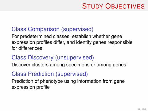
STUDY OBJECTIVES
Class Comparison (supervised)For predetermined classes, establish whether geneexpression profiles differ, and identify genes responsiblefor differences
Class Discovery (unsupervised)Discover clusters among specimens or among genes
Class Prediction (supervised)Prediction of phenotype using information from geneexpression profile
34 / 128

CLASS COMPARISON
Examples:
• Establish that expression profiles differ between twohistologic types of cancer
• Identify genes whose expression level is altered byexposure of cells to an experimental drug
35 / 128
CLASS COMPARISON
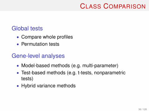
Global tests• Compare whole profiles• Permutation tests
Gene-level analyses
• Model-based methods (e.g. multi-parameter)• Test-based methods (e.g. t-tests, nonparametric
tests)• Hybrid variance methods
36 / 128
GLOBAL TESTS
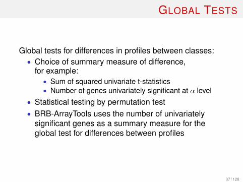
Global tests for differences in profiles between classes:• Choice of summary measure of difference,
for example:• Sum of squared univariate t-statistics• Number of genes univariately significant at α level
• Statistical testing by permutation test• BRB-ArrayTools uses the number of univariately
significant genes as a summary measure for theglobal test for differences between profiles
37 / 128

GENE-LEVEL
Model-based methodsMulti-parameter modeling of channel-level data (e.g.Gaussian mixed models), hierarchical Bayesian models,etc. May borrow information across genes and usemultiple comparison adjustments.
Test-based methodst-test, F-test, or Wilcoxon tests for each gene. Multiplecomparison adjustment commonly used.
Random variance methodsVariance estimates borrow across genes.
38 / 128

RANDOM VARIANCE
BayesianBaldi and Long, Bioinformatics, 2001
FrequentistWright and Simon, Bioinformatics, 2003Available as the ‘Random Variance’ option inBRB-ArrayTools
39 / 128
MULTIPLE TESTING
Goal:Identification of differentially expressed (DE) genes whilecontrolling for false discoveries (genes declared to bedifferentially expressed that in truth are not).
40 / 128

MULTIPLE TESTING
Don’tReject Reject
True Null U V m0
False Null T S m−m0
m−R R m
We compute m tests where m0 are true nulls and m−m0
are false nulls (DE).
The test rejects R out of m hypotheses, with S correctlyrejected. V represents a type I error and T represents atype II error. 7
7Adapted from Benjamini and Hochberg, JRSS-B, 1995.41 / 128

MULTIPLE TESTING
Different ways to control:
• Actual number of false discoveries: FD• Expected number of false discoveries: E(FD)• Actual proportion of false discoveries: FDP• Expected proportion of false discoveries:E(FDP) = false discovery rate (FDR)
FD = V and FDP = V/R
42 / 128

MULTIPLE TESTING: SIMPLE PROCEDURES
Control expected number of false discoveries
• E(FD) ≤ u
• conduct each of k tests at level u/k
Bonferroni control of family-wise error (FWE)
• Conduct each of k tests at level α/k• At least (1− α)100% confident that FD = 0
43 / 128
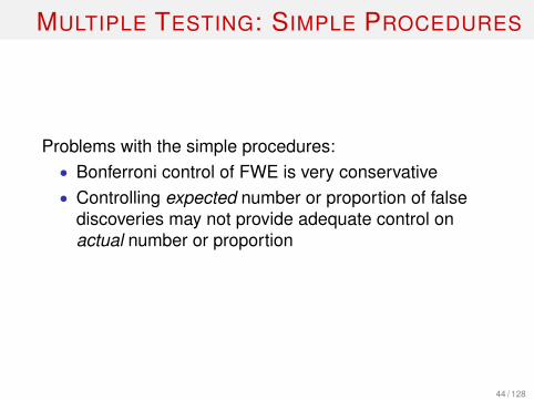
MULTIPLE TESTING: SIMPLE PROCEDURES
Problems with the simple procedures:• Bonferroni control of FWE is very conservative• Controlling expected number or proportion of false
discoveries may not provide adequate control onactual number or proportion
44 / 128

MULTIPLE TESTING
Additional Procedures:• Review by Dudoit et al. (Statistical Science, 2003)• “SAM” – Significance Analysis of Microarrays
• Tusher, et al., PNAS, 2001 and relatives• Esimate quantities similar to FDR (old SAM) or
control FDP (new SAM)• Bayesian
• Efron et al., JASA, 2001• Manduchi et al., Bioinformatics, 2000• Newton et al., J Comp Bio, 2001
• Step-down permutation procedures• Westfall and Young, 1993 Wiley (FWE)• Korn et al., JSPI, 2004 (FD and FDP control)
45 / 128

TYPES OF CONTROL
Korn et al. FDFD(2): We are 95% confident that the actual number offalse discoveries is not greater than 2
Korn et al. FDPFDP(0.10): We are 95% confident that the actualproportion of false discoveries does not exceed 0.10
Tusher et al. SAMSAMold(0.10): On average, the false discovery proportionwill be controlled at 0.10
Current SAMSAMnew(0.10): Similar to Korn FDP procedure
Bayesian MethodsHigher posterior probability of differential expression
46 / 128

MULTIPLE TESTING
The step-down permutation procedure for FD and FDPcontrol is available in BRB-ArrayTools for classcomparison, survival analysis, and quantitative traitsanalysis.
Can also set number of permutations
47 / 128

CLASS DISCOVERY
Examples:
• Discover previously unrecognized subtypes oflymphoma
• Cluster temporal gene expression patterns to getinsight into genetic regulation in response to a drugor toxin
48 / 128

CLASS DISCOVERY
Cluster Analysis
• Hierarchical• K-means• Self-organizing maps• Maximum likelihood/mixture models• Many more. . .
Graphical Displays
• Dendrogram• Heatmap• Multidimensional scaling plot
49 / 128

CLUSTER ANALYSIS
Hierarchical Agglomerative Clustering AlgorithmTwo approaches:
1 Cluster genes with respect to expression acrossspeciments
2 Cluster specimens with respect to gene expressionprofiles
Often helpful to filter genes that show little variationacross specimens and median/mean center genes.
50 / 128

CLUSTER ANALYSIS
Hierarchical Agglomerative Clustering AlgorithmMerge two “closest” observations into a cluster. Continuemerging closest clusters/observations.
Two things to define:1 How is distance between individuals measured?
• Euclidean• Maximum• Manhattan• 1 - Correlation
2 How is distance between clusters measured?• Average linkage• Complete linkage• Single linkage
51 / 128

DISTANCE METRICS
Euclidean distance:Measures absolute distance(square root of sum ofsquared differences)
1 - Correlation:Large values reflect lack oflinear association (patterndissimilarity)
Large Euclidean, Small 1 − Corr
Gene
Log 2
(Rat
io)
−0.4
−0.2
0.0
0.2
0.4
●
●
●●
●
●
●
●
●
●
●
● ●
●
1 2 3 4 5 6 7
Small Euclidean, Large 1 − Corr
Gene
Log 2
(Rat
io)
−0.4
−0.2
0.0
0.2
0.4
●
●
●
●●
●
●
●
●
● ●
●
●
●
1 2 3 4 5 6 7
52 / 128
LINKAGE METHODS
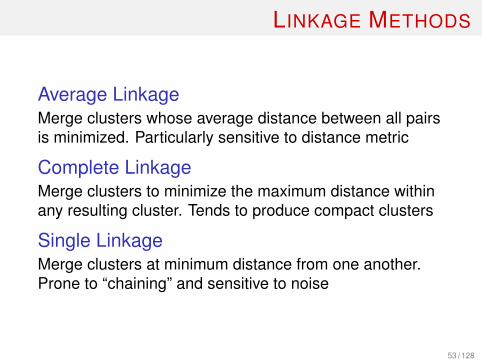
Average LinkageMerge clusters whose average distance between all pairsis minimized. Particularly sensitive to distance metric
Complete LinkageMerge clusters to minimize the maximum distance withinany resulting cluster. Tends to produce compact clusters
Single LinkageMerge clusters at minimum distance from one another.Prone to “chaining” and sensitive to noise
53 / 128

LINKAGE METHODS
Two Clusters
Single Linkage
Complete Linkage
Average Linkage
54 / 128

CLUSTER ANALYSISComplete
M91
.054
UA
CC
.091
UA
CC
.127
3M
93.0
07M
92.0
01U
AC
C.5
02U
AC
C.1
256 H
A.A
UA
CC
.152
9T
D.1
730
TD
.163
8T
D.1
720 TD
.138
4U
AC
C.1
022
TC
.137
6.3
TD
.137
6.3
TC
.F02
7U
AC
C.2
534
A.3
75U
AC
C.3
83U
AC
C.4
57U
AC
C.3
093
UA
CC
.109
7U
AC
C.6
47U
AC
C.1
012
M93
.47
UA
CC
.930
UA
CC
.287
3U
AC
C.9
03U
AC
C.8
27W
M17
91.C
0.2
0.4
0.6
0.8
1.0
Single
UA
CC
.903
M93
.47
TC
.F02
7U
AC
C.1
012
UA
CC
.647
UA
CC
.109
7H
A.A
UA
CC
.253
4U
AC
C.5
02A
.375
UA
CC
.125
6M
91.0
54M
92.0
01M
93.0
07U
AC
C.0
91U
AC
C.1
273
UA
CC
.383
UA
CC
.457
UA
CC
.309
3 TD
.138
4T
D.1
730
UA
CC
.102
2T
C.1
376.
3T
D.1
376.
3T
D.1
638
TD
.172
0U
AC
C.1
529
UA
CC
.827
WM
1791
.CU
AC
C.9
30U
AC
C.2
873
0.20
0.25
0.30
0.35
0.40
0.45
0.50
0.55
0.60
Average
M93
.47
UA
CC
.930
UA
CC
.287
3U
AC
C.9
03U
AC
C.1
097
TC
.F02
7U
AC
C.5
02M
92.0
01A
.375
UA
CC
.125
6M
91.0
54M
93.0
07U
AC
C.0
91U
AC
C.1
273
TD
.173
0T
D.1
638
TD
.172
0 TD
.138
4U
AC
C.1
022
TC
.137
6.3
TD
.137
6.3
UA
CC
.253
4U
AC
C.3
83U
AC
C.4
57U
AC
C.3
093
UA
CC
.647
UA
CC
.101
2U
AC
C.8
27W
M17
91.C
HA
.AU
AC
C.1
529
0.2
0.3
0.4
0.5
0.6
0.7
0.8
Dendrograms using 3different linkage methods,1 - Corr distance (Data fromBittner et al., Nature, 2000)
55 / 128

DOES CLUSTER METHOD MATTER?
56 / 128

CLUSTER ANALYSIS
How to interpret the cluster analysis results:• Cluster analyses always produce cluster structure
• Where to “cut” the dendrogram?• Which clusters do we believe?
• Circular reasoning• Clustering using only genes found significantly
different between two classes• “Validating” clusters by testing for differences
between subgroups observed to segregate in clusters
• Different clustering algorithms may find differentstructure using the same data
57 / 128
ASSESSING CLUSTERING RESULTS
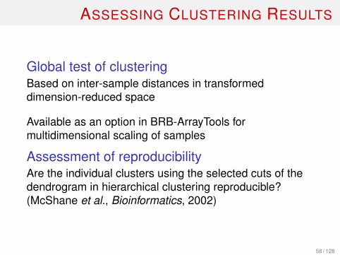
Global test of clusteringBased on inter-sample distances in transformeddimension-reduced space
Available as an option in BRB-ArrayTools formultidimensional scaling of samples
Assessment of reproducibilityAre the individual clusters using the selected cuts of thedendrogram in hierarchical clustering reproducible?(McShane et al., Bioinformatics, 2002)
58 / 128

ASSESSING CLUSTERING RESULTS
Data Perturbation MethodsMost believable clusters are those that persist given smallperturbations of the data.
Perturbations represent an anticipated level of noise ingene expression measurements.
Perturbed data sets are generated by adding randomerrors to each original data point:• Gaussian Errors –McShane et al., Bioinformatics,
2002• Bootstrap residual errors–Kerr and Churchill, PNAS,
2001
59 / 128
ASSESSING CLUSTERING RESULTS
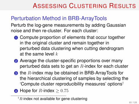
Perturbation Method in BRB-ArrayToolsPerturb the log-gene measurements by adding Gaussiannoise and then re-cluster. For each cluster:
1 Compute proportion of elements that occur togetherin the original cluster and remain together inperturbed data clustering when cutting dendrogramat the same level k
2 Average the cluster-specific proportions over manyperturbed data sets to get an R-index for each cluster
3 the R-index may be obtained in BRB-ArrayTools forthe hierarchical clustering of samples by selecting the‘Compute cluster reproducibility measures’ options†8
4 Hope for R-index ≥ 0.75
8†R-index not available for gene clustering60 / 128

R-INDEX EXAMPLE
X3
X1
X2
Y3
Y1
Y2
Z3
Z1
Z2
13
57
Original Data
X3
X1
X2
Z1
Z2
Y1
Y2
Y3
Z3
13
57
Perturbed Data
• 3 out or 3 pairs in X remain together• 3 out of 3 pairs in Y remain together• 1 out of 3 pairs in Z remain together• R = (3 + 3 + 1)/(3 + 3 + 3) = 0.78
61 / 128

CLUSTER REPRODUCIBILITY: MELANOMA
From Bittner et al., Nature, 2000. Expression profiles of31 melanomas were examined with a variety of classdiscovery methods.
A group of 19 melanomas consistently clustered together
62 / 128

CLUSTER REPRODUCIBILITY: MELANOMA
63 / 128

CLUSTER REPRODUCIBILITY: MELANOMA
For hierarchical clustering, the cluster of interest hadR-index = 1.0 (highly reproducible)
Melanomas in the 19 element cluster tended to have:• reduced invasiveness• reduced mortality
64 / 128

ESTIMATING NUMBER OF CLUSTERS
• GAP statistic (Tibshirani et al., JRSS B, 2002):detects too many false clusters (not recommended).
• Yeung et al. (Bioinformatics, 2001): jackknife method,estimate # of gene clusters.
• Dudoit et al. (Genome Biology, 2002):prediction-based resampling.
• Comparison of methods for estimating number ofclusters (Milligan and Cooper, Psychometrika, 1985):uncertain performance in high dimensions.
65 / 128

HEAT MAP
!"#$""% &%'&(&')*+ ,-./- 0*12+"03 4566"025%'&%7 #5 #8" (*6&*9!&+&#: &% 265+&;"6*#&5% &%'"< #8*# 8*0 !""% 26"(&5)0+: 5!0"6("' &%,-./-=>?@8" 150# 2651&%"%# '&0#&%4#&5% !"#$""% /-- *%' A- 4*1" ;651
7"%"0 #8*# *6" 48*6*4#"6&0#&4 5; 7"61&%*+ 4"%#6" . 4"++0 BA&7? =C? D%"<#"%0&(" 4+)0#"6 5; 7"%"0 '&0#&%7)&08"' 7"61&%*+ 4"%#6" . 4"++0 ;651!5#8 6"0#&%7 !+55' . 4"++0 *%' !" #!$%& *4#&(*#"' !+55' . 4"++0? @8&0 &06"1*6E*!+" !"4*)0" #8" 0#&1)+& )0"' #5 *4#&(*#" #8" !+55' . 4"++0$"6" 4850"% #5 1&1&4 #850" E%5$% #5 !" &1256#*%# ;56 7"61&%*+4"%#6" ;561*#&5%F 46500+&%E&%7 5; #8" &11)%57+5!)+&% 6"4"2#56 *%'/,GH 0&7%*++&%7? I5$"("63 &# 8*0 #8)0 ;*6 %5# !""% 2500&!+" #51&1&4"<*4#+: #8" 7"61&%*+ 4"%#6" 28"%5#:2" !" #!$%&3 *0 '"#"61&%"' !: #8";*&+)6" 5; * (*6&"#: 5; *4#&(*#&5% 45%'&#&5%0 #5 &%')4" #8" "<26"00&5%5; ./-9J 265#"&%3 * 8&78+: 02"4&K4 1*6E"6 ;56 7"61&%*+ 4"%#6" .
4"++0==? @8" 7"61&%*+ 4"%#6" .94"++ 7"%" "<26"00&5% 0&7%*#)6" 085$0#8*# 7"61&%*+ 4"%#6" . 4"++0 6"26"0"%# * '&0#&%4# 0#*7" 5; .94"++'&;;"6"%#&*#&5% *%' %5# 1"6"+: 5%" 02"4&K4 ;561 5; .94"++ *4#&(*#&5%?L)2256# ;56 #8&0 %5#&5% 451"0 ;651 #8" ;*4# #8*# #8" 48*6*4#"6&0#&47"%" "<26"00&5% 26576*1 5; 7"61&%*+ 4"%#6" . 4"++0 $*0 1*&%#*&%"'&% * 4)+#)6"' ,-./- 4"++ +&%" &% #8" *!0"%4" 5; #8" 7"61&%*+ 4"%#6"1&465"%(&65%1"%# BA&70 > *%' =C?@8" 5!0"6(*#&5% #8*# A-0 085$ * 2*##"6% 5; 5%75&%7 051*#&4
8:2"61)#*#&5% 5; &11)%57+5!)+&% 7"%"0 8*0 +"' #5 #8" 0)77"0#&5%#8*# #8" #6*%0;561*#&5% "("%# +"*'&%7 #5 A- 544)60 $8&+" #8" . 4"++ &0&% #8" 7"61&%*+ 4"%#6" 1&465"%(&65%1"%#=M? @8" 7"%" "<26"00&5%0&7%*#)6" 5; 7"61&%*+ 4"%#6" . 4"++0 $*0 6"265')4"' (&6#)*++:)%48*%7"' &% A-3 0)2256#&%7 #8" (&"$ #8*# #8&0 +:12851* *6&0"0;651 #8&0 0#*7" 5; .94"++ '&;;"6"%#&*#&5% BA&7? =C?
!"#$%&'(
ND@OPQ R ST- GHM R M AQ.PODPU =HHH R $$$?%*#)6"?451 )*)
OCI Ly3OCI Ly10DLCL-0042DLCL-0007DLCL-0031DLCL-0036DLCL-0030DLCL-0004DLCL-0029Tonsil Germinal Center BTonsil Germinal Center CentroblastsSUDHL6DLCL-0008DLCL-0052DLCL-0034DLCL-0051DLCL-0011DLCL-0032DLCL-0006DLCL-0049TonsilDLCL-0039Lymph NodeDLCL-0001DLCL-0018DLCL-0037DLCL-0010DLCL-0015DLCL-0026DLCL-0005DLCL-0023DLCL-0027DLCL-0024DLCL-0013DLCL-0002DLCL-0016DLCL-0020DLCL-0003DLCL-0014DLCL-0048DLCL-0033DLCL-0025DLCL-0040DLCL-0017DLCL-0028DLCL-0012DLCL-0021Blood B;anti-IgM+CD40L low 48hBlood B;anti-IgM+CD40L high 48hBlood B;anti-IgM+CD40L 24hBlood B;anti-IgM 24hBlood B;anti-IgM+IL-4 24hBlood B;anti-IgM+CD40L+IL-4 24hBlood B;anti-IgM+IL-4 6hBlood B;anti-IgM 6hBlood B;anti-IgM+CD40L 6hBlood B;anti-IgM+CD40L+IL-4 6hBlood T;Adult CD4+ Unstim.Blood T;Adult CD4+ I+P Stim.Cord Blood T;CD4+ I+P Stim.Blood T;Neonatal CD4+ Unstim.Thymic T;Fetal CD4+ Unstim.Thymic T;Fetal CD4+ I+P Stim.OCI Ly1WSU1JurkatU937OCI Ly12OCI Ly13.2SUDHL5DLCL-0041FL-9FL-9;CD19+FL-12;CD19+FL-10;CD19+FL-10FL-11FL-11;CD19+FL-6;CD19+FL-5;CD19+Blood B;memoryBlood B;naiveBlood BCord Blood BCLL-60CLL-68CLL-9CLL-14CLL-51CLL-65CLL-71#2CLL-71#1CLL-13CLL-39CLL-52DLCL-0009
2 1 0–1–2
4.0002.0001.0000.5000.250
DLBCLGerminal centre BNl. lymph node/tonsilActivated blood BResting/activated TTransformed cell linesFLResting blood BCLL
Germinal CentreB cell
Lymph node
T cell
Pan B cell
Activated B cell
Proliferation
A
G
!"#$%& ' !"#$%$&'"&%( &()*+#$",- ./ -#,# #01$#**"., 2%+%3 4#1"&+#2 %$# +'# !536 7"((".,
7#%*)$#7#,+* ./ -#,# #01$#**"., /$.7 586 7"&$.%$$%9 %,%(9*#* ./ :; *%71(#* ./ ,.$7%(
%,2 7%("-,%,+ (971'.&9+#*3 <'# 2#,2$.-$%7 %+ +'# (#/+ ("*+* +'# *%71(#* *+)2"#2 %,2
1$.="2#* % 7#%*)$# ./ +'# $#(%+#2,#** ./ -#,# #01$#**"., ", #%&' *%71(#3 <'#
2#,2$.-$%7 "* &.(.)$ &.2#2 %&&.$2",- +. +'# &%+#-.$9 ./ 7>?@ *%71(# *+)2"#2 A*##
)11#$ $"-'+ B#9C3 D%&' $.E $#1$#*#,+* % *#1%$%+# &4?@ &(.,# ., +'# 7"&$.%$$%9 %,2 #%&'
&.()7, % *#1%$%+# 7>?@ *%71(#3 <'# $#*)(+* 1$#*#,+#2 $#1$#*#,+ +'# $%+". ./
'9F$"2"G%+"., ./ H).$#*&#,+ &4?@ 1$.F#* 1$#1%$#2 /$.7 #%&' #01#$"7#,+%( 7>?@
*%71(#* +. % $#/#$#,&# 7>?@ *%71(#3 <'#*# $%+".* %$# % 7#%*)$# ./ $#(%+"=# -#,#
#01$#**"., ", #%&' #01#$"7#,+%( *%71(# %,2 E#$# 2#1"&+#2 %&&.$2",- +. +'# &.(.)$ *&%(#
*'.E, %+ +'# F.++.73 @* ",2"&%+#2I +'# *&%(# #0+#,2* /$.7 H).$#*&#,&# $%+".* ./ J38K +. L
A!8 +. M8 ", (.- F%*# 8 ),"+*C3 N$#9 ",2"&%+#* 7"**",- .$ #0&()2#2 2%+%3 O##
O)11(#7#,+%$9 P,/.$7%+"., /.$ /)(( 2%+%3
© 2000 Macmillan Magazines Ltd
Figure: Lymphoma data (Alizadeh et al., Nature, 2000) 66 / 128

MULTIDIMENSIONAL SCALING (MDS)
High-dimensional data points are represented in alower-dimensional space (e.g. 3D):• Principal components or optimization methods• Depends only on pairwise distances between points• “Relationships” need not be well-separated clusters
67 / 128

MULTIDIMENSIONAL SCALING
arrays was 830,000 as compared with 232,000 for those givinginadequate arrays (P ! 0.03).
Focusing on the tumor and FNA profiles from these fourpatients, we used a hierarchical clustering algorithm to group thesamples on the basis of similarities in gene expression. Fig. 4Arepresents a hierarchical clustering dendogram that displays thesesimilarities based on distances of the branches in a tree. All of therepeat FNAs cluster tightly together on the tree with their corre-sponding tumor sample from the same patient (all human breastsamples). The Ewing’s sarcoma samples form a completely sepa-
rate branch on the dendogram that can be easily observed on theright-hand side of the figure. Fig. 4B is a principal componentrepresentation of the same data in three-dimensional space clearlyshowing that the FNAs cluster with their tumors.
DISCUSSIONWe have reported previously that molecular markers can be
detected in cytospin preparations from repeat FNAs of primarytumors in breast cancer patients undergoing neoadjuvant ther-
Fig. 4 A, hierarchial cluster-ing dendogram for FNA-tumorpairs of four human breast can-cers and two Ewing’s sarcomaxenografts. B, principal compo-nent representation for FNA-tumor pairs of four humanbreast cancers and two Ewing’ssarcoma xenografts.
799Clinical Cancer Research
American Association for Cancer Research Copyright © 2002 on May 8, 2011clincancerres.aacrjournals.orgDownloaded from
Figure: Color = patient, large circle = tumor, small circle = FNA.Assersohn et al., Clinical Cancer Research, 2002.
68 / 128

CLASS PREDICTION
Examples:
• Predict from expression profiles which patients arelikely to experience severe toxicity from a new drugversus who will tolerate it well
• Predict which breast cancer patients will relapsewithin two years of diagnosis versus who will remaindisease free
69 / 128

CLASS PREDICTION METHODS
• Comparison of linear discriminant analysis, NNclassifiers, classification trees, bagging, and boosting:Tumor classification based on gene expression data(Dudoit, et al., JASA, 2002).
• Weighted voting method: distinguished betweensubtypes of human actue leukemia (Golub et al.,Science, 1999).
• Compound covariate prediction: distinguished betweenmutation positive and negative breast cancers(Hedenfalk et al., NEJM, 2001; Radmacher et al., J.Comp. Bio., 2002).
• Support vector machines: classified ovarian tissue asnormal or cancerous (Furey et al., Bioinformatics, 2000).
• Neural networks: distinguished among diagnosticsubcategories of small, round, blue cell tumors inchildren (Khan et al., Nature Medicine, 2001).
70 / 128

COMPOUND COVARIATE PREDICTOR (CCP)
• Select “differentially expressed” genes by two-samplet-test with small α.
CCPi = t1xi1 + t2xi2 + . . .+ tdxid
tj is the t-statistic for gene j,xij is the log expression measure for gene j insample i,d is the number of differentially expressed genes (atlevel α).
• Threshold of classification: midpoint of the CCPmeans for the two classes.
• Ref: Tukey. Controlled Clinical Trials, 1993;Radmacher et al., J. Comp. Bio., 2002.
71 / 128

CLASSIFICATION PITFALLS
• When number of potential features is much largerthan the number of cases (p >> n), one can alwaysfit a predictor to have 100% accuracy on the data setused to build it.
• If applied naively, more complex modeling methodsare more prone to over-fitting.
• Estimating accuracy by “plugging in” data used tobuild a predictor results in highly biased estimates ofperformance (re-substitution estimate).
• Internal and external validation of predictors areessential.
• Ref: Simon et al., JNCI, 2003; Radmacher et al., J.Comp. Bio., 2002.
72 / 128

OVER-FIT
0 2 4 6 8 10
46
810
1214
True Function
x
f (x)
73 / 128

OVER-FIT
0 2 4 6 8 10
46
810
1214
Sample of 5 observations
x
f (x)
●●
●
●
●
74 / 128

OVER-FIT
0 2 4 6 8 10
46
810
1214
Two Samples of 5 observations
x
f (x)
●●
●
●
●
●
●
●
●●
75 / 128

OVER-FIT
• Models in high dimension are usually complex (notnecessarily for the individual gene, but as a whole themodel has a large space to live in).
• Sample sizes are virtually always too small forprecise estimation of the true model.
• Look for simpler models that provide reasonableapproximations
76 / 128

OVER-FIT
In almost every experiment, we are interested in theperformance of the predictor on future (GeneralizationError) and not the performance of the predictor on thecurrent data (Resubstitution Error).
The difference between the generalization error and theresubstitution error is one measure of the over-fit.
77 / 128

VALIDATION APPROACHES
Internal ValidationWithin-sample Validation:• Cross-validation (many flavors: leave-one-out,
split-sample, k-fold, etc.)• Bootstrap and other resampling methods• See Molinaro et al. (Bioinformatics, 2005)
External ValidationIndependent-sample validation
78 / 128

LEAVE-ONE-OUT CV (LOOCV)
j
Samples
12⋮
j + 1⋮
N
j - 1
Build Classifier
Predict Class on j-th Sample
Compare True and Predicted
Class
Repeat for each j in 1, ... , N
79 / 128

INTERNAL VALIDATION
Limitations of within-sample validation:• Frequently performed incorrectly:
• Improper CV (e.g. not including feature selection)• Special statistical inference procedures required
(Lusa et al., Statistics in Medicine, 2007; Jiang et al.,Stat. Appl. Gen. and Mol. Bio., 2008).
• Large variance in estimated accuracy and effectsizes,
• Doesn’t protect against biases due to selectiveinclusion/exclusion of samples.
• Built-in biases possible (e.g. lab batch, specimenhandling).
80 / 128

PREDICTION SIMULATION
Generation of Gene Expression Profiles
• 100 specimens (Pi, i = 1, . . . , 100)• Log-ratio measurements on 6000 genes• Pi ∼ MVN(0, I6000)
• 1000 simulation repetitions• Can we distinguish between the first 50 speciments
(class 1) and the last 50 (class 2)? The classdistinction is artificial here since all 100 weregenerated from the same distribution.
Prediction MethodLinear Discriminant Analysis (LDA) prediction usingsignificant DE genes (α = 0.001).
81 / 128
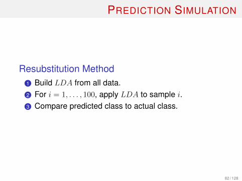
PREDICTION SIMULATION
Resubstitution Method1 Build LDA from all data.2 For i = 1, . . . , 100, apply LDA to sample i.3 Compare predicted class to actual class.
82 / 128

PREDICTION SIMULATION
LOOCV Without Gene Selection1 Select DE genes for LDA using all 100 samples.2 For i = 1, . . . , 100:
1 Leave out sample i.2 Build LDA(i) on other 99 samples.3 Apply LDA(i) to sample i.
3 Compare predicted class to actual class
83 / 128

PREDICTION SIMULATION
LOOCV with Gene Selection (Correct)1 For i = 1, . . . , 100:
1 Leave out sample i.2 Select DE genes based on other 99 samples.3 Build LDA(i) on other 99 samples.4 Apply LDA(i) to sample i.
2 Compare predicted class to actual class
84 / 128

PREDICTION SIMULATION
Misclassification estimate
density
0
2
4
6
8
0.0 0.2 0.4 0.6 0.8 1.0
group
LOOCV Correct
LOOCV Wrong
Resubstitution
85 / 128

BREAST CANCER EXAMPLE
Gene-Expression Profiles in Hereditary Breast Cancer(Hedenfalk et al., NEJM, 2001).• cDNA microarrays• Breast tumors studied
• 7 BRCA1+ tumors• 7 BRCA2+ tumors• 7 sporadic tumors
• Log-ratios measurements of 3226 genes for eachtumor after initial data filtering.
Research questionsCan we distinguich BRCA1+ from BRCA1- cancers andBRCA2+ from BRCA2- cancers — based solely on theirgene expression profiles?
86 / 128

BREAST CANCER EXAMPLE
Classification with Compound covariate predictor:910 11
Class # genes † # misclass (m) ‡ proportion §
BRCA1+/− 9 1 0.004BRCA2+/− 11 4 0.043
9†α = 0.0001 on the full data set10‡ Using LOOCV11§ Proportion of permutations with m or fewer misclassifications
87 / 128
CLASS PREDICTION IN BRB-ARRAYTOOLS
• Variety of prediction methods available• Predictors are automatically cross-validated, and a
significance test may be performed on thecross-validated mis-classification rate.
• Independent test samples may also be classifiedusing the predictors formed on the training set.
88 / 128

CLASS PREDICTION IN BRB-ARRAYTOOLS
89 / 128

CLASS PREDICTION IN BRB-ARRAYTOOLS
Additional prediction plug-ins:• Adaboost: Freund and Schapire, In Proceedings of
the Thirteenth Internal Conference on MachineLearning, 1996.
• Prediction Analysis of Microarrays (PAM): Tibshiraniet al., PNAS, 2002.
• Random Forests: Breiman, Machine Learning, 2001.• Top-scoring pairs: Geman et al., SAGMB, 2004.
90 / 128

1 Introduction: Technology
2 Data Quality & Image Processing
3 Normalization & Filtering
4 Study Objectives
5 Design Considerations
91 / 128

DESIGN CONSIDERATIONS
• Sample selection, including reference sample• Sources of variability/levels of replication• Pooling• Sample size planning• Controls• For 2-color spotted arrays:
• Reverse fluor experiments• Allocation of samples to array experiments
92 / 128

SAMPLE SELECTION
Experimental Samples
• A random sample from a population underinvestigation?
• Broad versus narrow inclusion criteria?
Reference Samples (cDNA)• In most cases, does not have to be biologically
relevant:• Expression of most genes, but not too high.• Same for every array
• Other situations exist (e.g. matched normal & cancer)
93 / 128

SOURCES OF VARIABILITY
4 3 6 | JUNE 2001 | VOLUME 2 www.nature.com/reviews/neuro
P E R S P E C T I V E S
needed to generate expression data from rawTIFF images. Furthermore, sharing of imagesbetween different platforms, such as shortoligonucleotide arrays and cDNA arrays, iscomplicated by the very different and in somecases,proprietary routines used to analyse thesignal.So,although flexible, this mode of shar-ing requires considerable effort on the part ofthe user. Until storage becomes cheaper andsoftware tools more ubiquitous, this level ofsharing cannot be considered mandatory.
and gives the investigator the possibility ofobtaining high-quality, retrospectively collecteddata.This would clearly satisfy biostatisticiansand mathematicians,and would provide maxi-mum flexibility for incorporation into meta-analyses of large numbers of experiments.
Sharing of raw images also requires thatusers have expertise in and tools for image anddata analysis. In many cases, either the end-user biologist or the statistician will lack accessto and experience using the software tools
The purpose of sharingThe best protocol for data sharing ultimatelydepends on how the data are to be used.Therewill be many individual specific reasons forsharing; here I consider three broad motiva-tions. The first is based on the fact that mostwell-conceived microarray experiments identi-fy dozens (if not hundreds) of genes of interestto a particular system or disease, only a few ofwhich can be studied by one laboratory.As thisinformation could lead to medical or scientificbreakthroughs, it is wasteful and potentiallyunethical for investigators to sequester or hidethis data,which could be most efficiently usedby several independent laboratories. The sec-ond reason for sharing data is related to theoften-small number of replications in any sin-gle experiment.One could obtain an increasedconfidence in results19 and an increase in ana-lytical flexibility by combining data from dif-ferent laboratories that are studying the samephenomenon.The third reason is to make dataavailable to mathematicians for the develop-ment of improved analytical methods, as wellas for comparisons of different array platformsand methodologies.Very little has been pub-lished comparing various platforms to showempirically their different strengths and weak-nesses.Together, these rationales provide com-pelling reasons why microarray data should beshared in centralized databases20.
Sharing paradigmsTo make array data useful to others, sharingparadigms have to be agreed upon a priori. Idiscuss four basic paradigms for sharingmicroarray data, each of which has advantagesand disadvantages: first, sharing the raw TIFF(tag information file format) images; second,sharing the extracted raw spot intensity valueswith background measurements; third, shar-ing the processed data, such as averaged inten-sity ratios; and last, sharing a list of genes thatshow clear differential expression. Thestrengths and limitations of each paradigm aresummarized in TABLE 1 and expanded below.
Sharing images. Sharing of the raw images isthe most flexible option, but this route posespractical limitations due to the size of theimages. Raw images allow re-analysis of theimage with different spot-definition algorithmsand background estimation,and they serve allthe sharing rationales listed above. The rawimages allow the application of different analyt-ical routines at almost every level, as well ascomprehensive examination of the image char-acteristics.As little has been published compar-ing various image-analysis, background-sub-traction and statistical approaches, sharingimages represents the most unbiased approach
Field
A
AAAAAAAA
MetaRow
1
11111111
MetaColumn
1
11111111
Row
1
11111111
Column
9
12345678
GeneID
Flag
0
20000000
Signal Mean
4845.895
977.03451682.4922119.4351636.9522801.6642790.2573134.1084461.877
BackgroundMean
2832.78
814.81911004.7831143.0381498.7211762.4781867.0172232.6252678.064
SignalMedian
4592
9661534114415672740270430174465
BackgroundMedian
2792
788992
112115001738186122062642
Signal Area
133
8765
124124107148
74114
BackgroundArea
749
503766208208913718723810
Signal Total
644504
86002109362262810202982299778412958231924508654
BackgroundTotal
2121752
409854769664237752311734
1609142134051816141882169232
SignalStdev
1180.442
197.2116557.9295
2140.42363.8378586.7534551.2724
602.175715.0632
Begin Raw Data
Wild-type mouse
Sample preparation
RNA extraction, labelling
Hybridization
cDNAcDNA
A B
Image scanning
False colour image representing greyscale values
Data analysis
Data mining / Database
Spotted mouse
Detectors
Laser
Slide
Figure 1 | Experimental stages in a typical cDNA microarray experiment. Total RNA is extractedfrom the two specimens to be compared (spotted and non-spotted brains) and cDNAs are separatelyreverse-transcribed and labelled with different fluorescent dyes. The two samples are co-hybridized on tothe array, a laser excites the dyes and a scanner collects and analyses the scattered light. The imagesproduced by each dye are co-registered and a false colour overlay is produced. In other platforms, suchas Affymetrix or radioactively probed arrays, only one sample is hybridized on to each array andcomparisons are made between arrays. Software is used to segment the raw image into spots,background and intensity values are obtained for each spot, and output is stored in table or tab-delimitedformat. Ratios of differential expression are calculated and various statistically or empirically derivedthresholds are used to classify spots as differentially expressed or not, usually by combining severalreplicate hybridizations. Data can be combined with other array data obtained under different conditionsor at different time points, and various data visualization and data exploration algorithms such asclustering or principal-components analysis are applied. Other data-mining approaches include using aset of coordinately regulated genes to identify novel or known promoter or enhancer regions that mightunderlie co-regulation. Given the number of steps involved in obtaining interpretable array data, it is nosurprise that differences in methodology at any step can introduce variability in experimental results. So, itis important to report the methods used to generate the data in a common language.
© 2001 Macmillan Magazines Ltd
• Biological heterogeneity inpopulation
• Specimen Collection/handlingeffects
• Biological heterogeneity inspecimen
• RNA extraction• RNA amplification• Fluor labeling• Hybridization• Scanning
1212Geschwind, Nature Reviews Neuroscience, 2001
94 / 128

LEVELS OF REPLICATION
Technical ReplicatesRNA sample divided into multiple aliquots and re-arrayed.
Biological replicatesUse a different human/animal for each array.
In cell culture experiments, re-grow the cells under thesame condition for each array (independent replication).
95 / 128

LEVELS OF REPLICATION
Summary:• Independent biological replicates are required for
valid statistical inference.• Maximizing biological replicates usually results in the
best power for class comparisons.• Technical replicates can be informative, e.g., for QC
issues.• But, systematic technical replication usually results in
a less efficient experiment.
96 / 128

IS POOLING ADVANTAGEOUS?
• If RNA samples are tiny, pooling is an alternative toamplification.
• If RNA samples big enough, then there is not usuallyan advantage unless arrays are very expensive andsamples very cheap.
• NO FREE LUNCH: pooling samples for each arraycan reduce the number of arrays needed to achievedesired precision and power, but this will come at theCOST of requiring that a larger number of biologicallydistinct samples be used.
• Single pool with many aliquots hybridized to arrays isNOT smart! inference requires independentreplication.
97 / 128
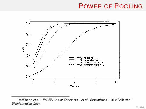
POWER OF POOLINGP1: GCRJournal of Mammary Gland Biology and Neoplasia (JMGBN) pp1035-jmgbn-475661 November 24, 2003 22:16 Style file version June 22, 2002
366 McShane, Shih, and Michalowska
Fig. 3. Power to detect a range of effect sizes (!/" ) when combining 2 independent specimens per pool, where " = SD of log2expression measurements for the gene within each group, and ! = true difference in mean log2 expression level between the twogroups. For all calculated values represented on the curves, significance level is set to 0.001, and the ratio of biological variance totechnical variance is set to 4. The number of independent biological samples per group is n/2.
when pooling specimens by pairs, 20 specimens (num-ber of arrays = 10) are required. Power could also becalculated for designs with pool sizes other than 2,but we will not present those additional calculationshere. There is a moderate effect of the ratio of biologi-cal to technical variance on these power comparisons.Consider the above selected design (effect size = 4,significance level = 0.001, 2 specimens per pool). Ifthe ratio is reduced to 1 (i.e., technical variance isequal to biological variance), then pooling results inpower 22%, 67%, and 93% when the original numberof specimens is equal to 12 (6 arrays), 16 (8 arrays),and 20 (10 arrays), respectively. In conclusion, pool-ing can result in substantial loss of power for detect-ing genes differentially expressed between groups andgenerally should be avoided unless necessary due toinsufficient amount of RNA available from individualsamples. If pooling is necessary for reasons of smallRNA samples or preferred due to the high cost of ar-rays, then the number of individual samples utilized
in the experiment should be increased appropriatelyto compensate for the decrease in power caused bypooling samples.
STATISTICAL ANALYSIS
The analysis of microarray data is a multistep pro-cess. First, there must be an analysis of the data quality,followed by calculation of gene-level summary statis-tics that have been suitably corrected and normalizedto remove noise due to experimental artifacts and tocorrect for systematic array and dye effects. Followingthis, the main analyses can be conducted to addressthe study aims.
Quality Screening
For either single-sample or dual-label arrays,there must be either visual or automated screening
13
13McShane et al., JMGBN, 2003; Kendziorski et al., Biostatistics, 2003; Shih et al.,Bioinformatics, 2004
98 / 128

ALLOCATION OF SPECIMENS
Allocation of speciments in cDNA array experiments forclass comparisons:• Reference design (traditional)• Balanced block design• All pairs design• Loop design (Kerr and Churchill, Biostatistics, 2001)
99 / 128

REFERENCE DESIGN
A1
R
RED
GREEN
Array 1
A2
R
Array 2
B1
R
Array 3
B2
R
Array 4
Ai = ith specimen from class A
Bi = ith specimen from class BR = aliquot from reference pool
100 / 128

REFERENCE DESIGN
If the reference sample is not biologically relevant to thetest samples, the class comparison is done betweengroups of arrays.
If the comparison between the reference sample and thetest samples is biologically meaningful (e.g. referencesample is a mixture of normal samples, test samples aretypes of tumor samples), the class comparison is donebetween green and red channels – some reverse fluorexperiments are required to adjust for potential dye bias.
101 / 128

BALANCED BLOCK DESIGN
A1B1
RED
GREEN
Array 1
B2A2
Array 2
A3B3
Array 3
B4A4
Array 4
Ai = ith specimen from class A
Bi = ith specimen from class B
102 / 128

ALLOCATION OF SPECIMENTS
• For 2-group comparisons, block design is mostefficient but precludes clustering.
• For cluster analysis or comparison of many groups,reference design is preferable.
• Reference design permits easiest analysis, allowsgreatest flexibility in making comparisons within andbetween experiments (using same reference), and ismost robust to technical difficulties.
• BRB-ArrayTools performs class comparison between“groups of arrays” (e.g. reference designs) orbetween “red and green channels” (e.g. blockdesigns).
103 / 128

SAMPLE SIZE PLANNING
For 2-group comparisons with cDNA arrays usingreference design or with Affymetrix arrays:• No comprehensive method for planning sample size
exists for gene expression profiling studies.• In lieu of such a method:
• Plan sample size based on comparisons of twoclasses involving a single gene.
• Make adjustments for the number of genes that areexamined.
104 / 128

SAMPLE SIZE PLANNING
Approximate total sample size required to compare twoequal sized, independent groups:
n =4σ2
(Zα/2 + Zβ
)δ2
Where:
δ = mean diff. between classes (log scale)σ = standard deviation (log scale)
Zα/2, Zβ = standard normal percentiles
More accurate iterative formulas recommended if n isapproximately 60 or less.
105 / 128

HOW TO CHOOSE α AND β
K = # of genes on array, M = # of genes DE at θ = 2δ
Expected number of false positives:
EFP ≤ (K −M)× α
Expected number of false negatives:
EFNθ =M × β
Popular choices for α and β: 14
α = 0.001 β = 0.05 or 0.10
141− β = Power106 / 128

EFFECT OF α AND β ON FDR
False Discovery Rate (FDR)is the expected proportion offalse-positive genes on thegene list
FDR =α(1− π)
α(1− π) + (1− β)π
where π is the proportion ofDE genes
π α 1− β FDR
0.005 0.01 0.95 68%0.005 0.01 0.80 71%0.005 0.001 0.95 17%0.005 0.001 0.80 20%0.05 0.001 0.95 2%
107 / 128

CHOOSING σ AND δ
Value of δ will be determined by biology and experimentalvariation. Within a single class, what SD is expected forexpression measure?
For log2 ratios, σ in range 0.25–1.0 (smallest for animalmodel and cell line experiments)
Value of δ is the size of mean difference (log2 scale) youwant to be able to detect:
2-fold: δ = log2(2) = 1
3-fold: δ = log2(3) = 1.59
108 / 128

SAMPLE SIZE EXAMPLE
K = 10,000 genes on arrayM = 100 genes DEα = 0.001 (Zα/2 = 3.291)
β = 0.05 (Zβ = 1.645)
σ = 0.75
δ = 1 (2-fold)
Need n = 55 (∼ 28 per group).
Expect ≤ 10 false positives and miss ≈ 5/100 2-foldgenes.
109 / 128

SAMPLE SIZE EXAMPLES (α = 0.001)
σ δ 2δ n Power(%)
0.25 1.00 2.00 6 950.50 1.00 2.00 14 950.25 1.00 2.00 5 820.50 1.00 2.00 5 140.25 1.20 2.29 5 950.50 2.39 5.24 5 95
15
15n is per group110 / 128

SAMPLE SIZE FOR CLASS PREDICTION
Raises unique issues:• The classes may mostly overlap, even in the high
dimensional space.• There may be no good classifier.• There will be an upper limit optimal performance that
no classifier can exceed.
Solution: Determine sample size big enough to get “closeto optimal” performance:• Dobbin and Simon, Biostatistics, 2007; Dobbin, Zhao
and Simon, Clin Cancer Res, 2008.• http://linus.nci.nih.gov/
111 / 128

SAMPLE SIZE FOR CLASS PREDICTION
3 essential inputs for sample size calculation with twoclasses:
1 Number of genes on the array2 The prevalence in each class3 The fold-change for informative genes (difference in
class means divided by within class SD, on the log2scale)
For example, ∼ 22, 000 features on the Affymetrix U113Aarray, 20% respond to drug, so prevalence is 20% vs.80%, and the fold change of 1.4.
112 / 128

SAMPLE SIZE FOR CLASS PREDICTION
113 / 128

SAMPLE SIZE FOR CLASS PREDICTION
114 / 128

SAMPLE SIZE REFERENCES
Technical replicates for 2 samples
• Lee et al., PNAS, 2000.• Black and Doerge, Bioinformatics, 2002.
Sample sizes for pooled RNA designs
• Shih et al., Bioinformatics, 2004.
Sample sizes for balanced block designs, paireddata, dye swaps, technical replicates, etc.
• Dobbin et al., Bioinformatics, 2003.• Dobbin and Simon, Biostatistics, 2005.
115 / 128

HOW BEST TO ALLOCATE EFFORT
• Microarrays can serve as a good high-throughputscreening tool to identify potentially interesting genes.
• Verification of results via a different, more accurate,assay often preferable to running many arrays ortechnical replicates.
• Gene IDs associated with sequences can changeover time, so periodic verification is advisable.
116 / 128

CONTROLS
Internal ControlsMultiple clones (cDNA arrays) or probe sets (Oligo arrays)for same gene spotted on array
External controlsSpiked controls (e.g. yeast or E. coli)
117 / 128

REVERSE FLUOR EXPERIMENTS
118 / 128

REVERSE FLUOR EXPERIMENTS
2-color spotted arrays with common referencedesignShould reverse fluor “replicates” be performed for everyarray? Usually NO!
See Dobbin, Shih and Simon, Bioinformatics, 2003 for acomprehensive discussion of reverse fluor replication.
119 / 128

REVERSE FLUOR EXPERIMENTS
When interested in interpreting individual ratios:• If gene-specific dye bias depends on gene sequence
and not sample characteristics, dye bias can beadjusted for by performing some reverse fluorexperiments.
• If dye bias depends on both the gene and thesample, dye swaps won’t help!
In BRB-ArrayTools, reverse fluor arrays must be specifiedduring the data importation (collation) step.
120 / 128

REVERSE FLUOR EXPERIMENTS
When interested in class comparisons and using commonreference design:• Comparing classes of non-reference samples tagged
with the same dye, the dye bias should cancel out.• Reverse fluors are not required.
121 / 128

REVERSE FLUOR EXPERIMENTS
When interested in class discovery and using commonreference design:• Usefulness of reverse fluor experiments and
replicates will depend on the nature and magnitude ofboth dye bias and experimental variability relative tobetween subject variability.
• For some clustering methods (e.g. Euclideandistance), constant dye biases should wash out.
• Some reverse fluors and replicates may be useful asinformal quality checks.
122 / 128

REVERSE FLUOR EXPERIMENTS
When interested in class prediction and using commonreference design:• Dye bias may wash out for some predictors (e.g.
nearest neighbors)• Dye bias may be incorporated into some predictors
(e.g. CCP)
123 / 128

REVERSE FLUOR EXPERIMENTS
Balanced Block Design
• For each class, half the samples should be taggedwith Cy3 and half with Cy5.
• When comparing different classes, dye bias willcancel out of the class comparisons.
• No reverse fluors are required.
124 / 128

SUMMARY I
• Data quality assessment and pre-processing areimportant.
• Different study objectives will require differentstatistical analysis approaches.
• Different analysis methods may produce differentresults. Thoughtful application of multiple methodsmay be required.
• Chances for spurious findings are enormous, andvalidation of any findings on larger independentcollections of specimens will be essential.
125 / 128
SUMMARY II
• Analysis tools can’t compensate for poorly designedexperiments.
• Fancy analysis tools don’t necessarily outperformsimple ones.
• Even the best analysis tools, if appliedinappropriately, can produce incorrect or misleadingresults.
126 / 128

HELPFUL WEBSITES
• NCI: http://linus.nci.nih.gov/brb• BRB-ArrayTools:http://linus.nci.nih.gov/BRB-ArrayTools.html
• BRB textbook:http://linus.nci.nih.gov/~brb/book.html
• PDF of this talk: http://linus.nci.nih.gov/~brb/presentations.htm
• Bioconductor: http://www.bioconductor.org/
127 / 128

ACKNOWLEDGEMENTS
• Richard Simon• Joanna Shih• Kevin Dobbin• Michael Radmacher• Members of the NCI Biometric Research Branch• Our NCI collaborators and students in the NIH
microarray classes• BRB-ArrayTools development team
128 / 128