Measuring Gene Expression Part 3 Key Steps in Microarray ...
51
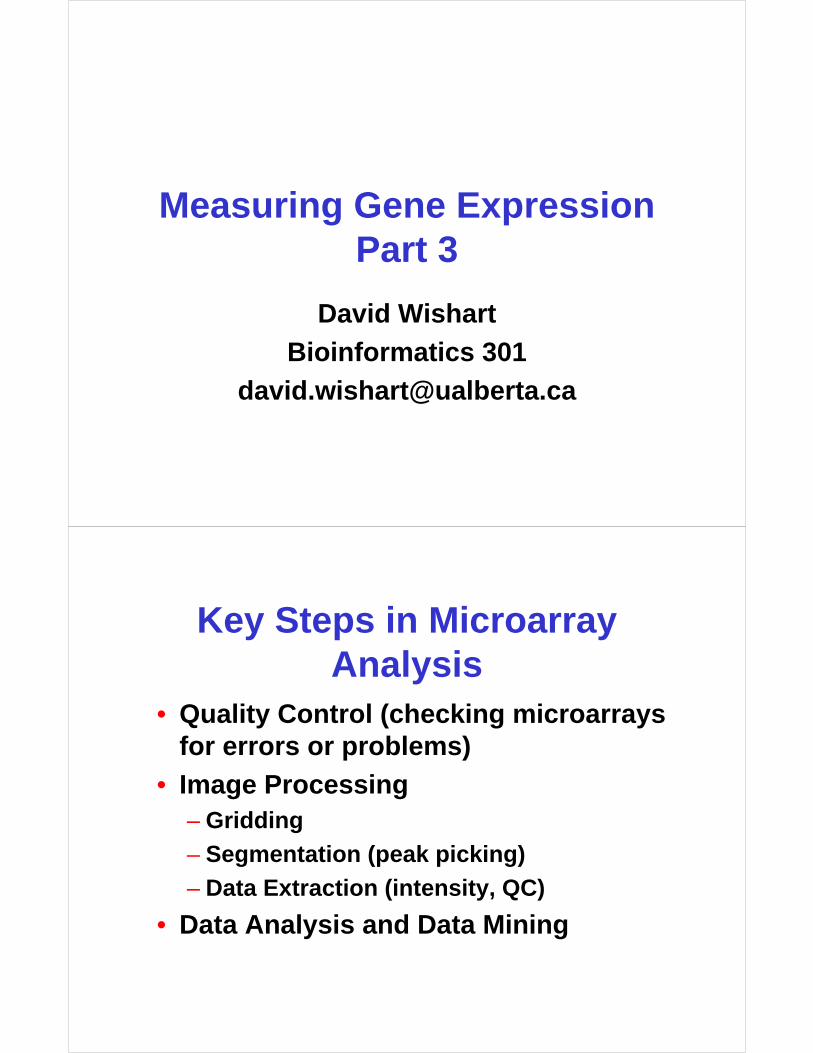
Measuring Gene Expression Part 3 David Wishart Bioinformatics 301 [email protected] Key Steps in Microarray Analysis • Quality Control (checking microarrays for errors or problems) • Image Processing – Gridding – Segmentation (peak picking) – Data Extraction (intensity, QC) • Data Analysis and Data Mining
-
Upload
khangminh22 -
Category
Documents
-
view
5 -
download
0
Transcript of Measuring Gene Expression Part 3 Key Steps in Microarray ...
Measuring Gene Expression Part 3
David Wishart
Bioinformatics 301
Key Steps in MicroarrayAnalysis
• Quality Control (checking microarraysfor errors or problems)
• Image Processing– Gridding
– Segmentation (peak picking)
– Data Extraction (intensity, QC)
• Data Analysis and Data Mining

Comet Tailing
• Often caused by insufficiently rapid immersion of the slides in the succinic anhydride blocking solution.
Uneven Spotting/Blotting
• Problems with print tips or with overly viscous solution
• Problems with humidity in spottiing chamber

High Background
• Insufficient Blocking
• Precipitation of labelled probe
Gridding Errors
Spotting errors
Gridding errors
Uneven hybridization

Key Steps in MicroarrayAnalysis
• Quality Control (checking microarraysfor errors or problems)
• Image Processing– Gridding
– Segmentation (spot picking)
– Data Extraction (intensity, QC)
• Data Analysis and Data Mining
Microarray Scanning
Laser
PMT
Dye
Glass Slide
Objective Lens
Detector lens
Pinhole
Beam-splitter

Microarray Principles
overlay images and normalize
Laser 1 Laser 2
Scan and detect withconfocal laser system
Image process and analyze
Green channel
Red channel
Microarray Images
• Resolution– standard 10µm [currently, max 5µm]– 100µm spot on chip = 10 pixels in diameter
• Image format– TIFF (tagged image file format) 16 bit (64K grey
levels)– 1cm x 1cm image at 16 bit = 2Mb (uncompressed)– other formats exist i.e. SCN (Stanford University)
• Separate image for each fluorescent sample– channel 1, channel 2, etc.

Image Processing
• Addressing or gridding– Assigning coordinates to each of the spots
• Segmentation or spot picking– Classifying pixels either as foreground or as
background
• Intensity extraction (for each spot)– Foreground fluorescence intensity pairs (R, G)
– Background intensities
– Quality measures
Gridding

Gridding Considerations
• Separation between rows and columns of grids
• Individual translation of grids
• Separation between rows and columns of spots within each grid
• Small individual translation of spots
• Overall position of the array in the image
• Automated & manual methods available
Spot Picking
• Classification of pixels as foreground or background (fluorescence intensities determined for each spot are a measure of transcript abundance)
• Large selection of methods available, each has strengths & weaknesses

Spot Picking
• Segmentation/spot picking methods:– Fixed circle segmentation
– Adaptive circle segmentation
– Adaptive shape segmentation
– Histogram segmentation
ImaGene, QuantArraym DeArray and adaptive thresholdingHistogram method
Spot, region growing and watershedAdaptive shape
GenePix, DappleAdaptive circle
ScanAlyze, GenePix, QuantArrayFixed circle
Fixed Circle Segmentation
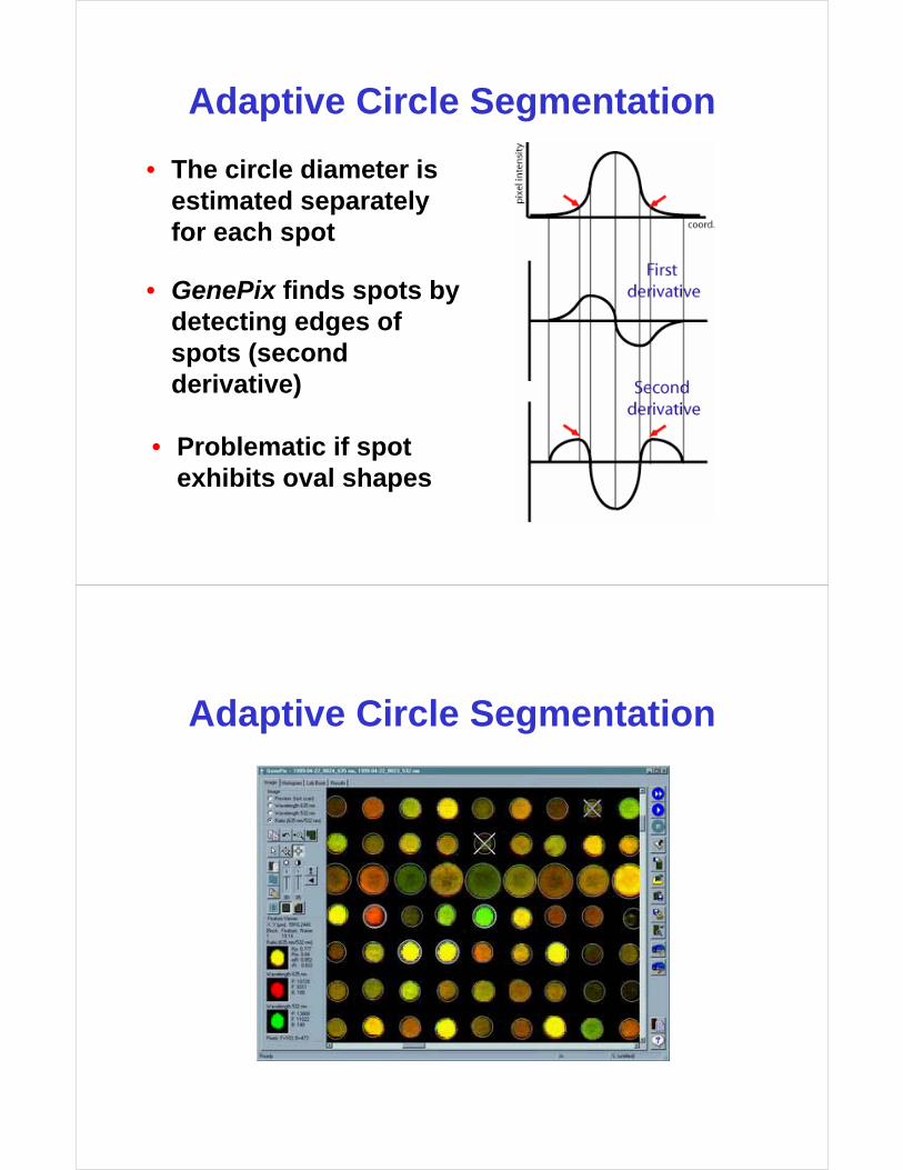
Adaptive Circle Segmentation
• The circle diameter is estimated separately for each spot
• GenePix finds spots by detecting edges of spots (second derivative)
• Problematic if spot exhibits oval shapes
Adaptive Circle Segmentation

Adaptive Shape Segmentation
Edge detection or Seeded Region Growing(R. Adams and L. Bishof (1994) - Regions grow outwards from the seed points preferentially according to the difference between a pixel’s value and the running mean of values in an adjoining region
Information Extraction
• Spot Intensities• mean (pixel intensities)
• median (pixel intensities)
• Background values• Local Background
• Morphological opening
• Constant (global)
• Quality Information Take the average

Spot Intensity• The total amount of hybridization for a spot
is proportional to the total fluorescence at the spot
• Spot intensity = sum of pixel intensities within the spot mask
• Since later calculations are based on ratios between cy5 and cy3, we compute the average* pixel value over the spot mask
• Can use ratios of medians instead of means
Means vs. Medians
row col ch1_sig_mea ch2_sig_mea ch1_sig_med ch2_sig_med
1 1 56000 2000 58000 1900
1 2 1000 600 600 800
1 3 2000 60000 3000 59000
etc.

Mean, Median & Mode
ModeMedian
Mean
Mean, Median, Mode
• In a Normal Distribution the mean, mode and median are all equal
• In skewed distributions they are unequal
• Mean - average value, affected by extreme values in the distribution
• Median - the “middlemost” value, usually half way between the mode and the mean
• Mode - most common value

Background Intensity
• A spot’s measured intensity includes a contribution of non-specific hybridization and other chemicals on the glass
• Fluorescence intensity from regions not occupied by DNA can be different from regions occupied by DNA
Local Background Methods• Focuses on small regions around spot mask
• Determine median pixel values in this region
• Most common approach
ScanAlyze ImaGene Spot, GenePix
• By not considering the pixels immediately surrounding the spots, the background estimate is less sensitive to the performance of the segmentation procedure

Local Background Methods
Quality Measurements
• Array– Correlation between spot intensities
– Percentage of spots with no signals
– Distribution of spot signal area
– Inter-array consistency
• Spot– Signal / Noise ratio
– Variation in pixel intensities
– ID of “bad spots” (spots with no signal)

A Microarray Scatter Plot
Cy3 (green) intensity
Cy
5 (r
ed
) in
ten
sity
Correlation
Cy3 (green) intensity
Cy
5 (r
ed
) in
ten
sity
Cy3 (green) intensity
Cy
5 (r
ed
) in
ten
sity
Linear Non-linear
Comet-tailing from non-balanced channels

Correlation
“+” correlation Uncorrelated “-” correlation
Correlation
Highcorrelation
Lowcorrelation
Perfectcorrelation

Correlation Coefficient
r = 0.85 r = 0.4 r = 1.0
r = Σ(xi - µx)(yi - µy)
Σ(xi - µx)2(yi - µy)2
Correlation Coefficient
• Sometimes called coefficient of linear correlation or Pearson product-moment correlation coefficient
• A quantitative way of determining what model (or equation or type of line) best fits a set of data
• Commonly used to assess most kinds of predictions or simulations

Correlation and Outliers
Experimental error orsomething important?
A single “bad” point can destroy a good correlation
Outliers
• Can be both “good” and “bad”
• When modeling data -- you don’t like to see outliers (suggests the model is bad)
• Often a good indicator of experimental or measurement errors -- only you can know!
• When plotting gel or microarray expression data you do like to see outliers
• A good indicator of something significant

Log Transformation
linear scale log2 scale
ch1 intensity0
10000
20000
30000
40000
50000
60000
70000
0 10000 20000 30000 40000 50000 60000 70000
ch2
inte
nsity
exp’t Aexp’t A
0
2
4
6
8
10
12
14
16
18
0 5 10 15ch1 intensity
Choice of Base is Not Important
0
1
2
3
4
5
6
0 2 4 6
0
2
4
6
8
10
12
14
0 5 10 15
log10 ln
exp’t Aexp’t A

Why Log2 Transformation?
• Makes variation of intensities and ratios of intensities more independent of absolute magnitude
• Makes normalization additive
• Evens out highly skewed distributions
• Gives more realistic sense of variation
• Approximates normal distribution
• Treats up- and down- regulated genes symmetrically
log2 ch1 intensity
log 2
ch2
inte
nsity
16
16
0
Applying a log transformation makes the variance and offset more proportionate along the entire graph
ch1 ch2 ch1/ch2
60 000 40 000 1.5
3000 2000 1.5
log2 ch1 log2 ch2 log2 ratio
15.87 15.29 0.58
11.55 10.97 0.58
Log Transformations

Log Transformations
0 8000 16000 24000 32000 40000 48000 56000 6400
V5
0
0
0
0
0
8.0 8.8 9.6 10.4 11.2 12.0 12.8 13.6 14.4 15.2 16.0
V4
0.0
0.1
0.2
0.3
0.4
0.5
log transformed
exp’t Blinear scale
exp’t B
Log Transformation

Normalization• Reduces systematic (multiplicative)
differences between two channels of a single hybridization or differences between hybridizations
• Several Methods:– Global mean method
– (Iterative) linear regression method
– Curvilinear methods (e.g. loess)
– Variance model methods
Try to get a slope ~1 and a correlation of ~1
Example Where Normalization is Needed
1) 2)

Example Where Normalization is Not Needed
1) 2)
Normalization to a Global Mean
• Calculate mean intensity of all spots in ch1 and ch2– e.g. µch2 = 25 000 µch2/µch1 = 1.25
– µch1 = 20 000
• On average, spots in ch2 are 1.25X brighter than spots in ch1
• To normalize, multiply spots in ch1 by 1.25

Hypothetical Data
Ch 1 Ch 2 Ch1 + Ch2
0
2
4
6
8
10
12
14
16
18
0 2 4 6 8 10 12 14 16 18
ch1 log2 signal intensity
ch2
log 2
sign
al in
tens
ity
log(µch1 ) = 10.88
log(µch2 ) = 11.72
log(µch2 - µch1)= 0.84
y = x
y = x + 0.84
Pre-normalized Data

0
2
4
6
8
10
12
14
16
18
0 2 4 6 8 10 12 14 16 18
Add 0.84 to every value in ch1 to normalize
ch1 log2 signal intensity
ch2
log 2
sign
al in
tens
ity
y = ƒ(x)ƒ(x)= x + 0.84
y = x
Normalized Microarray Data
fit a line (y=mx+b) to the data set
set aside outliers (residuals > 2 x s.d.)
repeat until r2
changes by< 0.001
then apply slope and intercept to
the original dataset
Finkelstein et al. (2001) www.camda.edu
Normalization by Iterative Linear Regression

log2 Cy3
log 2
Cy5
0
Channel 1 vs. 2 – Raw Data
log2 Cy3
log 2
Cy5
0
Ch. 1 vs. 2 – Outlier Removal

log 2
Cy5
0
signal vs. signal : pre normalization
log2 Cy3
log 2
Cy5
Ch. 1 vs. 2 – Outlier Removal
log 2
Cy5
0
log2 Cy3
Ch. 1 vs. 2 – Slope Adjust
log 2
Cy5
0
log2 Cy3
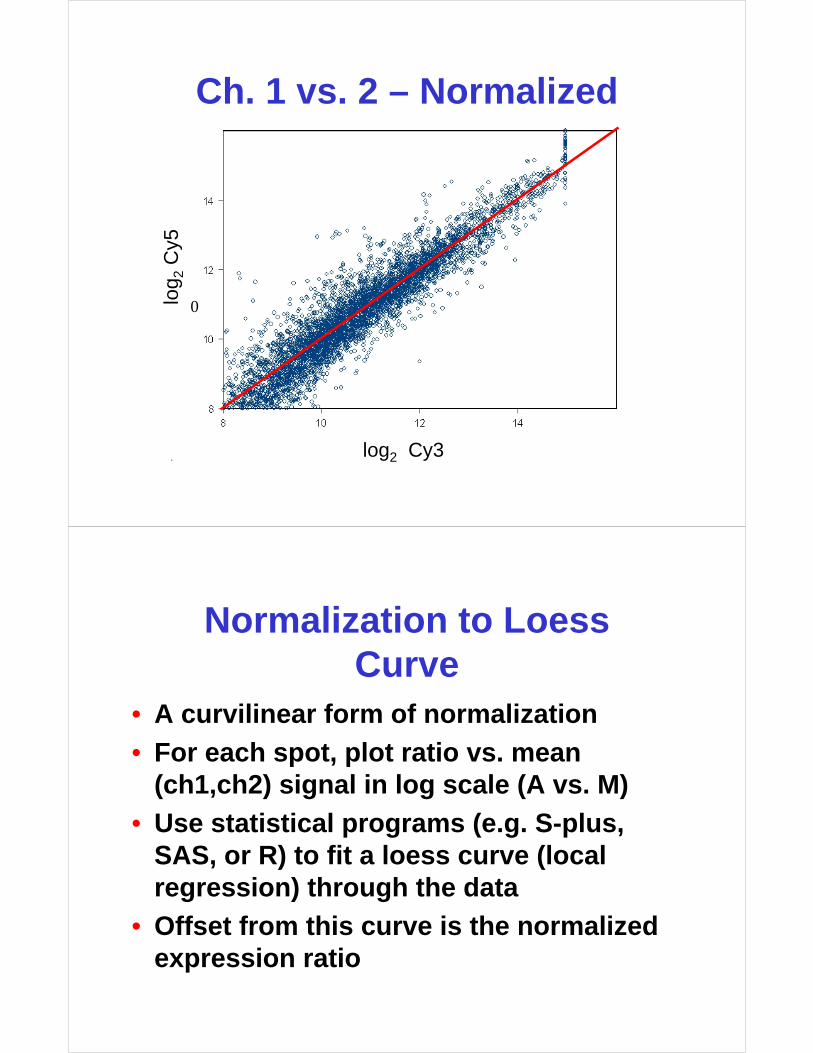
Ch. 1 vs. 2 – Normalized
Normalization to Loess Curve
• A curvilinear form of normalization
• For each spot, plot ratio vs. mean (ch1,ch2) signal in log scale (A vs. M)
• Use statistical programs (e.g. S-plus, SAS, or R) to fit a loess curve (local regression) through the data
• Offset from this curve is the normalized expression ratio

The A versus M Plot
A = 1/2 log2 (R*G)
More Informative Graph
M =
log
2(R
/G)
A vs. M PlotMore Informative Graph
M =
log
2(R
/G)
A = 1/2 log2 (R*G)

Prior To NormalizationNon-normalized data {(M,A)}n=1..5184:
M = log2(R/G)
Global (Loess) Normalization
average signal {log2 (Cy3 + Cy5)/2}
rati
o {
log 2
(Cy5
/ C
y3)}
0
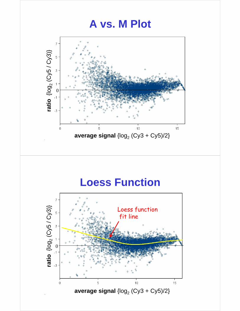
A vs. M Plot
average signal {log2 (Cy3 + Cy5)/2}
rati
o {
log 2
(Cy5
/ C
y3)} Loess function
fit line
0
Loess Function

average signal {log2 (Cy3 + Cy5)/2}
rati
o {
log 2
(Cy5
/ C
y3)}
0
Data After Normalization
Print-tip Normalization 16151413
1211109
8765
4321
Print-tip layout

Spatial NormalizationNo normalization Global normalization
Print-tip normalization Scaled Print-tip normalization
Quality Measurements
• Array– Correlation between spot intensities
– Percentage of spots with no signals
– Distribution of spot signal area
– Inter-array consistency
• Spot– Signal / Noise ratio
– Variation in pixel intensities
– ID of “bad spots” (spots with no signal)
Quality Assessment
OK quality High quality
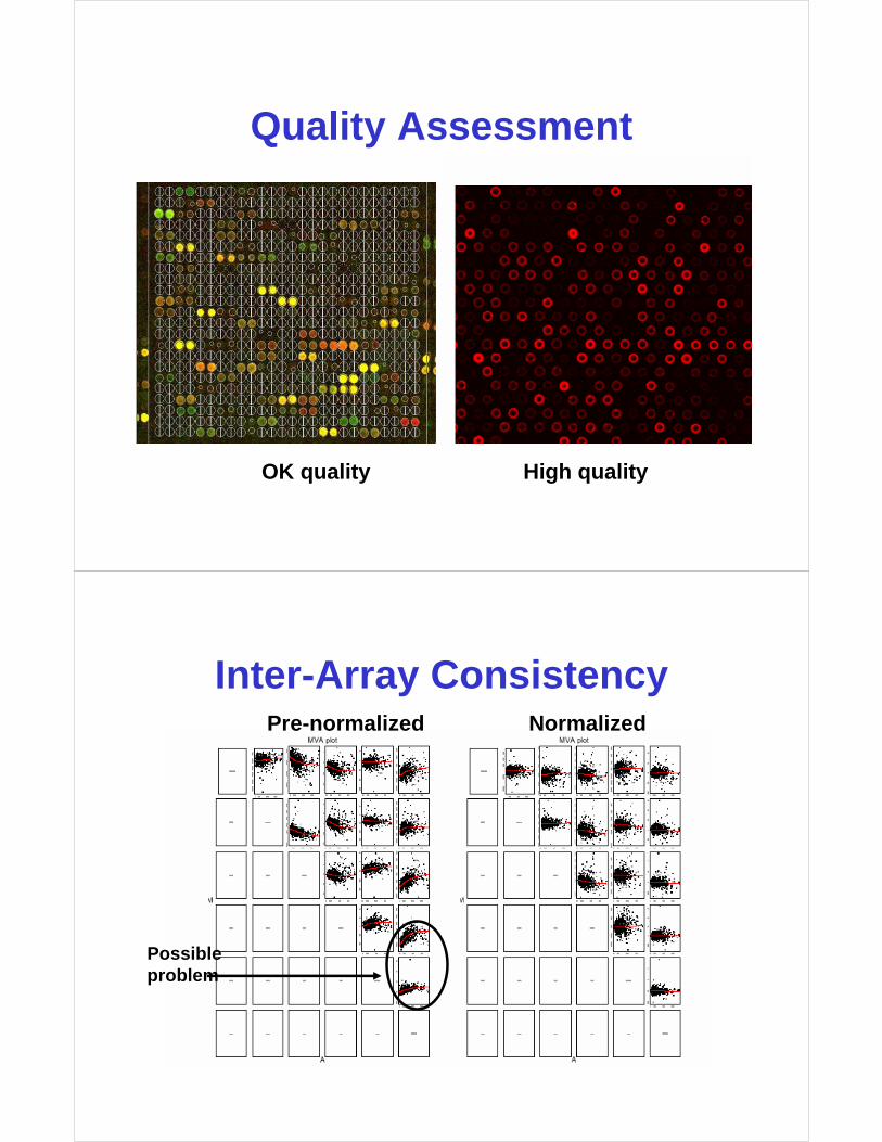
Inter-Array Consistency
Possibleproblem
Pre-normalized Normalized

Quality Assessment
High Quality Array
High Quality Array
Good Quality Array
Poor Quality Array
Poor Quality Array
1) R=1 95%CI=(1-1) N=82582) R=0.99 95%CI=(0.99-1) N=83323) R=0.99 95%CI=(0.99-0.99) N=8290
1) R=0.98 95%CI=(0.98-0.98) N=76942) R=0.97 95%CI=(0.97-0.98) N=78733) R=0.97 95%CI=(0.97-0.97) N=7694
1) R=0.7 95%CI=(0.68-0.72) N=20272) R=0.65 95%CI=(0.62-0.67) N=28183) R=0.61 95%CI=(0.59-0.64) N=2001
1) R=0.66 95%CI=(0.62-0.69) N=10282) R=0.86 95%CI=(0.85-0.87) N=19253) R=0.64 95%CI=(0.61-0.68) N=1040
1) R=0.49 95%CI=(0.44-0.54) N=9422) R=0.81 95%CI=(0.8-0.83) N=17003) R=0.57 95%CI=(0.52-0.61) N=973
Microarrays in Practice
• 14,352 spots from a collection of synthetic DNA 70mers from Operon
• Each oligo is spotted 2x side-by-side
• Each slide is prepared and scanned in triplicate (6 spots per gene)
• Each slide image is hand inspected & QCd
• Scanning system is calibrated by hand
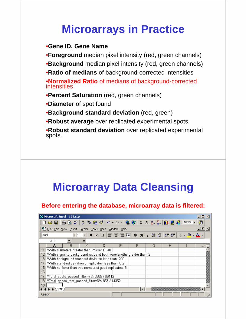
Microarrays in Practice•Gene ID, Gene Name
•Foreground median pixel intensity (red, green channels)
•Background median pixel intensity (red, green channels)
•Ratio of medians of background-corrected intensities
•Normalized Ratio of medians of background-corrected intensities
•Percent Saturation (red, green channels)
•Diameter of spot found
•Background standard deviation (red, green)
•Robust average over replicated experimental spots.
•Robust standard deviation over replicated experimental spots.
Microarray Data Cleansing
Before entering the database, microarray data is filtered:

• Purpose is to set aside spots with low, high, or negative intensity values– low intensity values are associated with
high variance (a sensitivity issue)
– very high signals may be saturated
– negative signals can be produced by background subtraction
Data Filtering/Cleansing
Final Result
Trx 16.8Enh1 13.2Hin2 11.8P53 8.4Calm 7.3Ned3 5.6P21 5.5Antp 5.4Gad2 5.2Gad3 5.1Erp3 5.0
GPD 0.11Shn2 0.13Alp4 0.22OncB 0.23Nrd1 0.25LamR 0.26SetH 0.30LinK 0.32Mrd2 0.32Mrd3 0.33TshR 0.34
Highly Exp Reduced Exp
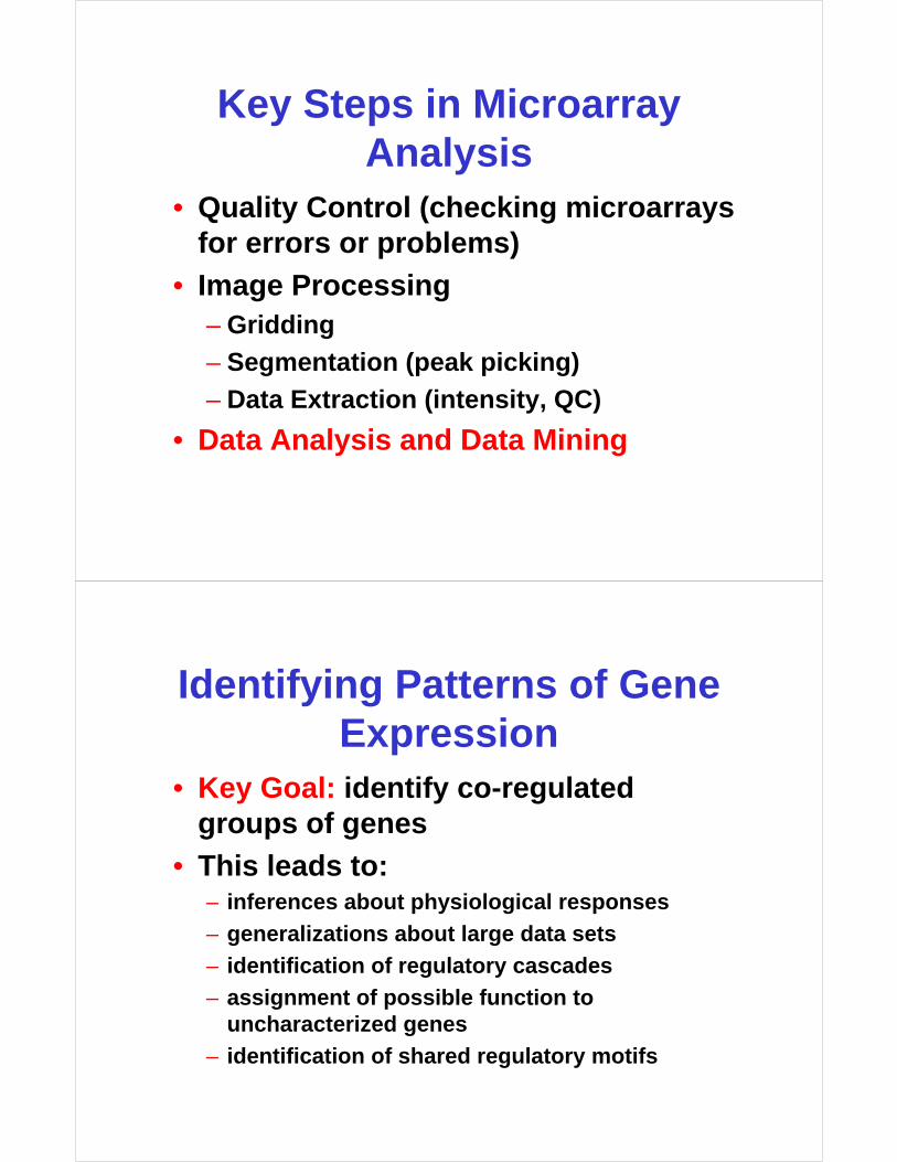
Key Steps in MicroarrayAnalysis
• Quality Control (checking microarraysfor errors or problems)
• Image Processing– Gridding
– Segmentation (peak picking)
– Data Extraction (intensity, QC)
• Data Analysis and Data Mining
Identifying Patterns of Gene Expression
• Key Goal: identify co-regulated groups of genes
• This leads to:– inferences about physiological responses
– generalizations about large data sets
– identification of regulatory cascades
– assignment of possible function to uncharacterized genes
– identification of shared regulatory motifs

Analysis Methods
• Hierarchical clustering
• K-means clustering
• Self organizing feature maps
• Support vector machines
• Neural networks
• Principle Component Analysis
• Data Mining & Data Enrichment
Detecting Clusters
Weight
Hei
gh
t

Is it Right to Calculate a Correlation Coefficient?
Weight
Hei
gh
t
r = 0.73
Or is There More to This?
Weight
Hei
gh
t
female
male

Clustering Applications in Bioinformatics
• Microarray or GeneChip Analysis
• 2D Gel or ProteinChip Analysis
• Protein Interaction Analysis
• Phylogenetic and Evolutionary Analysis
• Structural Classification of Proteins
• Protein Sequence Families
Clustering
• Definition - a process by which objects that are logically similar in characteristics are grouped together.
• Clustering is different than Classification
• In classification the objects are assigned to pre-defined classes, in clustering the classes are yet to be defined
• Clustering helps in classification

Clustering Requires...
• A method to measure similarity (a similarity matrix) or dissimilarity (a dissimilarity coefficient) between objects
• A threshold value with which to decide whether an object belongs with a cluster
• A way of measuring the “distance”between two clusters
• A cluster seed (an object to begin the clustering process)
Clustering Algorithms
• K-means or Partitioning Methods - divides a set of N objects into M clusters -- with or without overlap
• Hierarchical Methods - produces a set of nested clusters in which each pair of objects is progressively nested into a larger cluster until only one cluster remains
• Self-Organizing Feature Maps - produces a cluster set through iterative “training”
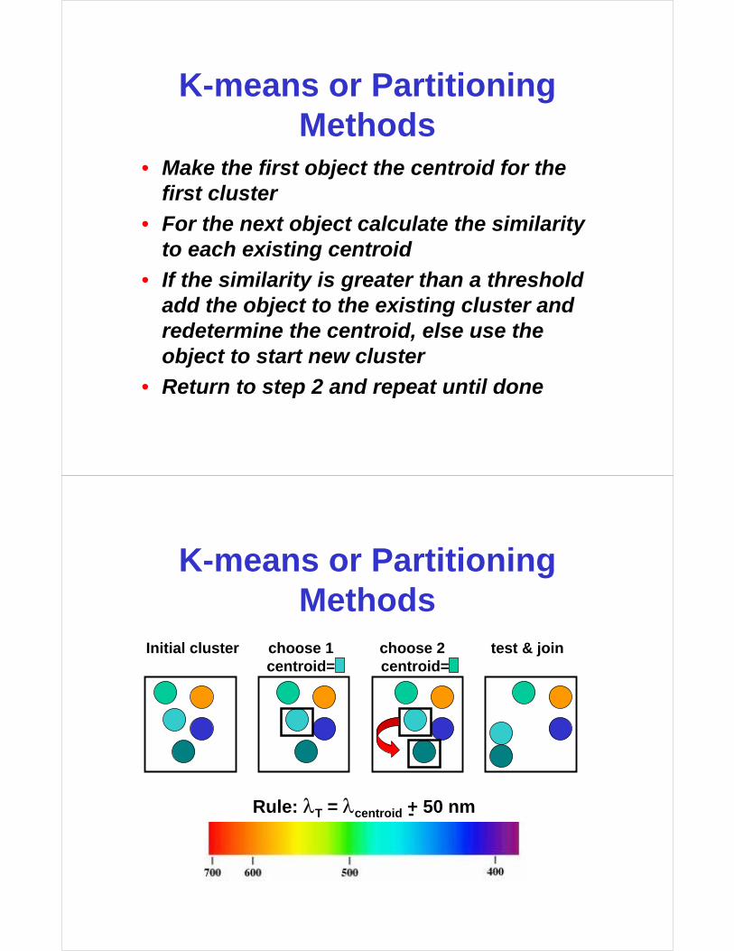
K-means or Partitioning Methods
• Make the first object the centroid for the first cluster
• For the next object calculate the similarity to each existing centroid
• If the similarity is greater than a threshold add the object to the existing cluster and redetermine the centroid, else use the object to start new cluster
• Return to step 2 and repeat until done
K-means or Partitioning Methods
Rule: λT = λcentroid + 50 nm-
Initial cluster choose 1 choose 2 test & joincentroid= centroid=
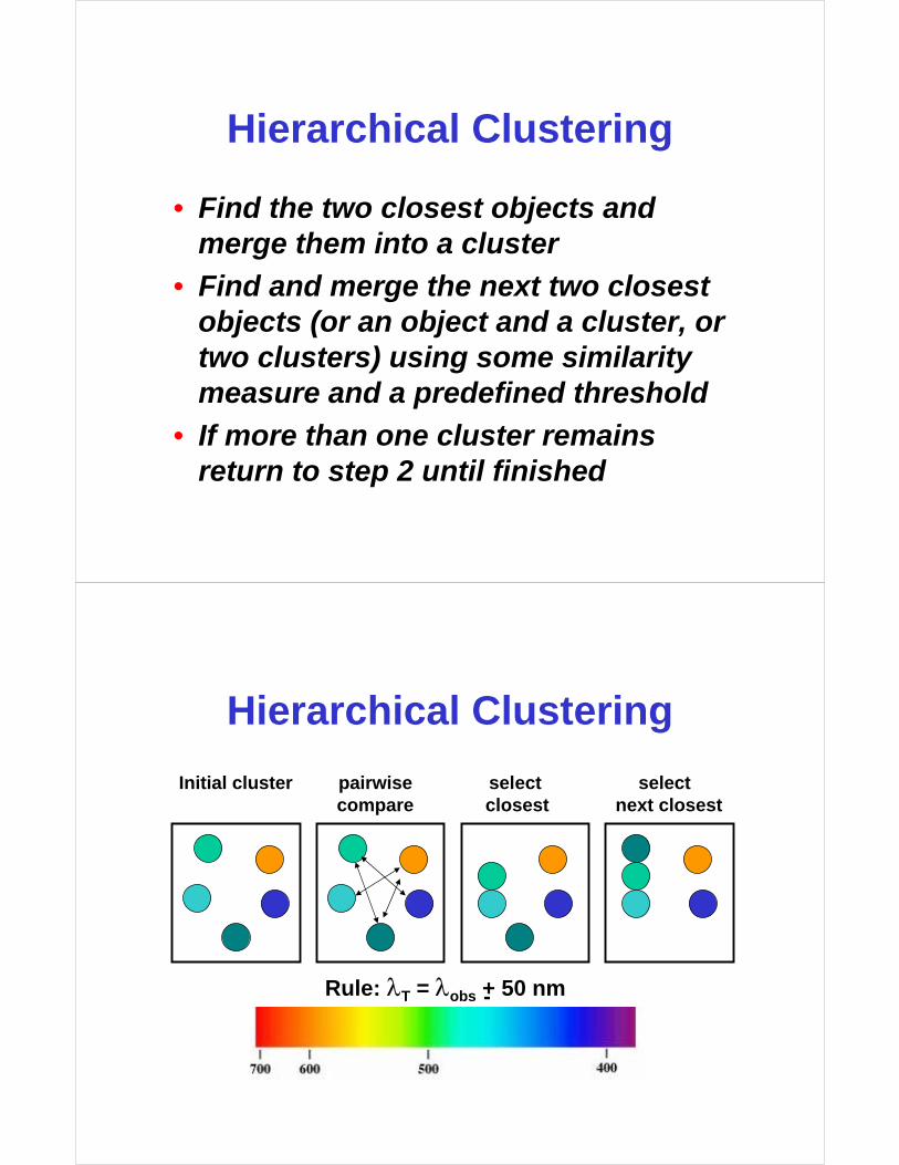
Hierarchical Clustering
• Find the two closest objects and merge them into a cluster
• Find and merge the next two closest objects (or an object and a cluster, or two clusters) using some similarity measure and a predefined threshold
• If more than one cluster remains return to step 2 until finished
Hierarchical Clustering
Rule: λT = λobs + 50 nm-
Initial cluster pairwise select selectcompare closest next closest

Hierarchical Clustering
Find 2 mostsimilar geneexpress levelsor curves
Find the nextclosest pairof levels orcurves
Iterate
A
B
B
A
C
A
B
C
D
E
F
Results

Self-Organizing Feature Maps
T=0 T=10 h
T=20 h T=30 h
Self-Organizing Feature Maps
Cluster 1 Cluster 2
Cluster 4Cluster 3
Cluster 6Cluster 5
Plot Chip Data Compute Feature Examine Clusters forMap with 6 nodes Biological Meaning

Data Mining
The Genomic Abyss
Data Mining
• Enriches the data content of previously collected experimental data -- adds to data dimemsionality
• Adds “prior knowledge” to raw or hard-to-interpret data
• Key to finding new relations or hidden connections
• Key to enhancing quality of predictions

Data Mining Challenges
• Terabytes of data “out there, somewhere”
• Data is constantly being updated,corrected
• New genes being added, old ones deleted
• Data sources are highly distributed
• Data sources are of variable quality (errors)
• Data is in various forms (image, numeric, natural language text, temporal, spatial)
• “mining a moving target”
Data Mining Solutions
• Use web-based agents (web-bots) to collect, compare and update data
• Identify key (reliable) databases
• Identify key “data fields” of interest or potential importance
• Generate a web-based, web-accessible ArrayCard to link genetic, metabolic, proteomic data to geneID

Mining Microarray Data
GenBank ID, UniGene ID
GenBank Website
UniGene Website
LocusLink Website
Entrez Nucleotide Website
Gene Sequence, CDS
Locus ID
Function, Cyto, GO, etc.
mRNA sequence, featre
Mining Microarray Data
LocusLink Website
GeneCard Website
GDB Website
SWISS-PROT Website
Bind Website
GeneCard ID
SNP data
SWISS-PROT ID
Length, name, MW, etc
Interacting partners

Putting it All Together
• Use clustering methods to identify unusual patterns or groups that associate with a disease state or conditions
• Use data mining to interpret the results in terms of existing biological or physiological knowledge
• Or selectively combine mined data with expression data to conduct further clustering
GenePublisher
http://www.cbs.dtu.dk/services/GeneMachine/

Microarray Protocols & Links
• http://www.microarrays.org/protocols.html
• http://brownlab.stanford.edu/protocols.html
• http://oz.Berkeley.EDU/users/terry/zarray/Html/
• http://ihome.cuhk.edu.hk/~b400559/arraysoft.html
http://genome-www5.Stanford.EDU/MicroArray//SMD/resinfo.html
• http://www.bio.davidson.edu/courses/genomics/chip/chip.html