Stabilizing Highly Dynamic Locomotion in Planar Bipedal Robots with

Dimension Reducing Control

by

Benjamin J. Morris

A dissertation submitted in partial fulfillmentof the requirements for the degree of

Doctor of Philosophy(Electrical Engineering: Systems)

in The University of Michigan2008

Doctoral Committee:Professor Jessy W. Grizzle, ChairProfessor N. Harris McClamrochAssociate Professor Daniel P. FerrisAssociate Professor Richard B. Gillespie

c© Benjamin J. Morris 2008All Rights Reserved

With love and thanks to my parents, Jim and Annette, for theirendless support

ii

ACKNOWLEDGMENTS

As my time at Michigan draws to a close, I would like to thank a number of individuals, without whom the work of

this thesis could not have been completed. First and foremost, I would like to wholeheartedly thank my advisor, Jessy

Grizzle, for his continual inspiration and intellectual support throughout my time at the University of Michigan. In our

conversations he has consistently valued theoretical insight and mathematical curiosity over the status quo of meetings,

reports, and paperwork. In my time as a graduate student, I have been allowed the freedom to explore a number of

research paths, many of which are contained in this thesis, but many more of which were dead ends. For Jessy’s patience

as a teacher, for his invitation to participate in the running experiments on RABBIT in France, and for his selfless interest

in my career development, I am grateful. Secondly, and with equal enthusiasm I would like to thank Eric Westervelt

for his roles as collaborator, co-author, travel companion, and friend throughout my years at the university, especially

during the 2005-2006 academic year that produced the conference and journal papers addressing the control of passive

dynamics within the framework of hybrid zero dynamics. Withthe many drafts of our coauthored papers, Eric has

helped shape the style of my professional writing. I am indebted to my fellow coauthors Eric Westervelt, Jessy Grizzle,

Christine Chevallereau, and Jun Ho Choi for the recently published book “Feedback Control of Dynamic Bipedal Robot

Locomotion” to which I am truly honored to have contributed.I would like to thank Jonathan Hurst, Al Rizzi, and Matt

Mason of Carnegie Mellon University for their contributions in the construction of the series compliant robotic prototypes

that have helped shape the direction of our theoretical research here at Michigan. For graciously tutoring me in RHexLib

and Ubuntu Linux and for setting up our initial computational framework for realtime control, Joel Chestnutt deserves

special thanks. In addition, the willing and capable programming expertise of Koushil Sreenath at the University of

Michigan has been invaluable throughout the last semester.Lastly, I would like to thank my family and close friends,

who through a combination of encouragement and prodding have helped bring this document to completion.

Benjamin Morris

December 2007

iii

TABLE OF CONTENTS

DEDICATION . . . . . . . . . . . . . . . . . . . . . . . . . . . . . . . . . . . . . . . . . ii

ACKNOWLEDGMENTS . . . . . . . . . . . . . . . . . . . . . . . . . . . . . . . . . . . iii

LIST OF TABLES . . . . . . . . . . . . . . . . . . . . . . . . . . . . . . . . . . . . . . . vii

LIST OF FIGURES . . . . . . . . . . . . . . . . . . . . . . . . . . . . . . . . . . . . . . viii

CHAPTERS

1 Introduction . . . . . . . . . . . . . . . . . . . . . . . . . . . . . . . . . . . . . 11.1 Why Study Bipedal Locomotion? . . . . . . . . . . . . . . . . . . . . . . 11.2 Bottom-up Techniques of Control . . . . . . . . . . . . . . . . . . . .. . 31.3 Context and Motivation . . . . . . . . . . . . . . . . . . . . . . . . . . . 41.4 Organization of Dissertation . . . . . . . . . . . . . . . . . . . . . .. . 7

2 Survey of Related Literature . . . . . . . . . . . . . . . . . . . . . . . . .. . . . 92.1 Formal Stability Analysis . . . . . . . . . . . . . . . . . . . . . . . . .. 102.2 The Zero Moment Point Criterion . . . . . . . . . . . . . . . . . . . . .132.3 Passive Dynamics and Minimal Actuation . . . . . . . . . . . . . .. . . 152.4 Marc Raibert . . . . . . . . . . . . . . . . . . . . . . . . . . . . . . . . 16

3 Technical Background . . . . . . . . . . . . . . . . . . . . . . . . . . . . . . .. 183.1 Systems with Impulse Effects . . . . . . . . . . . . . . . . . . . . . . .. 183.2 Periodic Orbits . . . . . . . . . . . . . . . . . . . . . . . . . . . . . . . 203.3 Poincare Return Map . . . . . . . . . . . . . . . . . . . . . . . . . . . . 203.4 Hybrid Invariance and Restriction Dynamics . . . . . . . . . .. . . . . . 233.5 Notions of Relative Degree . . . . . . . . . . . . . . . . . . . . . . . . .25

4 Models of Walking and Running in Planar Bipeds with Rigid Links . . . . . . . . 284.1 Model Hypotheses . . . . . . . . . . . . . . . . . . . . . . . . . . . . . 294.2 Phases of Motion . . . . . . . . . . . . . . . . . . . . . . . . . . . . . . 30

4.2.1 Flight Dynamics . . . . . . . . . . . . . . . . . . . . . . . . . . 304.2.2 Stance Dynamics . . . . . . . . . . . . . . . . . . . . . . . . . . 304.2.3 Landing Map . . . . . . . . . . . . . . . . . . . . . . . . . . . . 314.2.4 Liftoff Map . . . . . . . . . . . . . . . . . . . . . . . . . . . . . 324.2.5 Double Support Phase . . . . . . . . . . . . . . . . . . . . . . . 334.2.6 Coordinate Relabeling . . . . . . . . . . . . . . . . . . . . . . . 34

iv

4.3 Open-Loop Models of Walking and Running . . . . . . . . . . . . . .. . 35

5 Running Experiments with RABBIT: Six Steps toward Infinity. . . . . . . . . . 395.1 Controller Derivation . . . . . . . . . . . . . . . . . . . . . . . . . . . .41

5.1.1 Summary and Philosophy . . . . . . . . . . . . . . . . . . . . . 415.1.2 Parameterized Control with Impact Updated Parameters . . . . . 415.1.3 Parameterized Virtual Constraints . . . . . . . . . . . . . . .. . 425.1.4 Stance Phase Control . . . . . . . . . . . . . . . . . . . . . . . . 425.1.5 Flight Phase Control . . . . . . . . . . . . . . . . . . . . . . . . 435.1.6 Transition Control: Landing . . . . . . . . . . . . . . . . . . . . 445.1.7 Transition Control: Takeoff . . . . . . . . . . . . . . . . . . . . .445.1.8 Resulting Closed-Loop Model of Running . . . . . . . . . . . .. 455.1.9 Existence and Stability of Periodic Orbits . . . . . . . . .. . . . 46

5.2 Design of Running Motions with Optimization . . . . . . . . . .. . . . . 475.2.1 Optimization Parameters . . . . . . . . . . . . . . . . . . . . . . 475.2.2 Boundary Conditions of the Virtual Constraints . . . . .. . . . . 475.2.3 Optimization Algorithm Details . . . . . . . . . . . . . . . . . .485.2.4 An Example Running Motion . . . . . . . . . . . . . . . . . . . 49

5.3 Experiment . . . . . . . . . . . . . . . . . . . . . . . . . . . . . . . . . 515.3.1 Hardware Modifications to RABBIT . . . . . . . . . . . . . . . . 515.3.2 Result: Six Running Steps . . . . . . . . . . . . . . . . . . . . . 52

5.4 Conclusion . . . . . . . . . . . . . . . . . . . . . . . . . . . . . . . . . 545.5 Supplemental Material . . . . . . . . . . . . . . . . . . . . . . . . . . . 55

6 Sample-Based HZD Control for Robustness and Slope Invariance of Planar PassiveBipedal Gaits . . . . . . . . . . . . . . . . . . . . . . . . . . . . . . . . . . . . . 61

6.1 Model of Walking on Sloped Ground . . . . . . . . . . . . . . . . . . . .636.1.1 A System with Impulse Effects . . . . . . . . . . . . . . . . . . . 636.1.2 Example Model: A Two-Link Walker . . . . . . . . . . . . . . . 65

6.2 HZD Framework for the Control of Walking on Sloped Ground. . . . . . 666.2.1 Defining Virtual Constraints . . . . . . . . . . . . . . . . . . . . 666.2.2 A Feedback yielding Continuous Phase Invariance . . . .. . . . 676.2.3 The HZD of Walking . . . . . . . . . . . . . . . . . . . . . . . . 686.2.4 Gait Stability . . . . . . . . . . . . . . . . . . . . . . . . . . . . 706.2.5 Effects of Varying Ground Slope . . . . . . . . . . . . . . . . . . 71

6.3 Analysis of a Dynamic Singularity . . . . . . . . . . . . . . . . . . .. . 726.3.1 Singularity in the Decoupling Matrix . . . . . . . . . . . . . .. 736.3.2 A Closed Form Inverse . . . . . . . . . . . . . . . . . . . . . . . 746.3.3 Interpretations . . . . . . . . . . . . . . . . . . . . . . . . . . . 756.3.4 Approaching a Dynamic Singularity . . . . . . . . . . . . . . . .776.3.5 Example 1: A Singularity for the Two-Link Walker . . . . .. . . 78

6.4 Development of Additional Tools for the HZD Framework . .. . . . . . 796.4.1 Sample-Based Virtual Constraints . . . . . . . . . . . . . . . .. 796.4.2 Augmentation Functions . . . . . . . . . . . . . . . . . . . . . . 816.4.3 Example 2: Sampling a Torque Specified Gait . . . . . . . . . .. 82

6.5 Applications to the Control of Passive Bipedal Gaits . . .. . . . . . . . . 836.5.1 Control of Passive Walking . . . . . . . . . . . . . . . . . . . . . 83

v

6.5.2 Example 3: Enlarging the Basin of Attraction of a Stable, PassiveGait of a Two-link Biped . . . . . . . . . . . . . . . . . . . . . . 85

6.5.3 Example 4: Demonstration of Robustness to External Force Per-turbations and Mass and Inertia Variations . . . . . . . . . . . . . 86

6.5.4 Example 5: Changing the Minimum Slope Capability of a Motion 876.6 Conclusions . . . . . . . . . . . . . . . . . . . . . . . . . . . . . . . . . 88

7 A Restricted Poincare Map for Determining ExponentiallyStable Periodic Orbitsin the Presence of Smooth Transverse Dynamics . . . . . . . . . . . .. . . . . . 93

7.1 Coordinate Dependent Hypotheses and Stability Test . . .. . . . . . . . 947.2 Coordinate-Free Hypotheses and Stability Test . . . . . . .. . . . . . . . 977.3 Feedback Design to Meet Stability Hypotheses . . . . . . . . .. . . . . 997.4 Case Study: RABBIT Walking on Flat Ground . . . . . . . . . . . . .. . 100

7.4.1 Open-Loop Model . . . . . . . . . . . . . . . . . . . . . . . . . 1017.4.2 Feedback Design . . . . . . . . . . . . . . . . . . . . . . . . . . 1017.4.3 Closed-Loop Analysis . . . . . . . . . . . . . . . . . . . . . . . 1037.4.4 Numerical Simulation . . . . . . . . . . . . . . . . . . . . . . . 105

7.5 Discussion . . . . . . . . . . . . . . . . . . . . . . . . . . . . . . . . . . 105

8 Parameter Updates for Achieving Impact Invariance . . . . . .. . . . . . . . . . 1118.1 Definition and Properties of Parameter Extensions . . . . .. . . . . . . . 1128.2 Nonconstructive Parameter Extensions for Hybrid Invariance . . . . . . . 1138.3 Constructive Parameter Extensions for Hybrid Invariance . . . . . . . . . 1168.4 Discussion . . . . . . . . . . . . . . . . . . . . . . . . . . . . . . . . . . 119

9 Case Study: A Biped with Compliance Walking on Flat Ground .. . . . . . . . . 1229.1 Benefits and Drawbacks of Compliance . . . . . . . . . . . . . . . . .. 1249.2 A Biped with Uniform Series Compliant Actuation . . . . . . .. . . . . 1259.3 Model Properties . . . . . . . . . . . . . . . . . . . . . . . . . . . . . . 1279.4 An Application of Theorem 8.2 on Nonconstructive Extensions . . . . . . 1299.5 An Application of Theorem 8.6 on Constructive Extensions . . . . . . . . 1329.6 Discussion . . . . . . . . . . . . . . . . . . . . . . . . . . . . . . . . . . 140

10 Concluding Remarks . . . . . . . . . . . . . . . . . . . . . . . . . . . . . . . .. 14210.1 Summary of New Contributions . . . . . . . . . . . . . . . . . . . . . .14210.2 Perspectives on Future Work . . . . . . . . . . . . . . . . . . . . . . .. 144

APPENDIX . . . . . . . . . . . . . . . . . . . . . . . . . . . . . . . . . . . . . . . . . . . 146

BIBLIOGRAPHY . . . . . . . . . . . . . . . . . . . . . . . . . . . . . . . . . . . . . . . 161

vi

LIST OF TABLES

Table5.1 Terms of optimization. . . . . . . . . . . . . . . . . . . . . . . . . . . . .. . . . 505.2 Flight phase durations for the six running steps. . . . . . .. . . . . . . . . . . . . 556.1 Parameters of the two-link model. . . . . . . . . . . . . . . . . . . .. . . . . . . 667.1 Eigenvalues ofDP ǫ for three values ofǫ . . . . . . . . . . . . . . . . . . . . . . . 1079.1 Parameters of the five-link model with compliant actuation. . . . . . . . . . . . . . 123

vii

LIST OF FIGURES

Figure1.1 A picture of the AMASC actuator and a diagram of its potential use in a biped. . . 63.1 Geometric interpretation of a Poincare return map for an ODE (non-hybrid) system. 223.2 Geometric interpretation of a Poincare return map for asystem with impulse effects. 224.1 A simplifying coordinate convention. . . . . . . . . . . . . . . .. . . . . . . . . . 304.2 An illustration of leg swapping. . . . . . . . . . . . . . . . . . . . .. . . . . . . . 345.1 RABBIT and the different phases of running with coordinate conventions labeled. . 405.2 Stick diagram and Poincare map for the example running motion (rate 0.58 m/s). . 515.3 Estimated height of RABBIT’s point feet during the reported running experiment. . 535.4 Normalized gait parameter showing the existence of six running steps. . . . . . . . 565.5 Actuator saturation during running. . . . . . . . . . . . . . . . .. . . . . . . . . . 575.6 Joint tracking performance during running. . . . . . . . . . .. . . . . . . . . . . 585.7 Joint tracking error during running. . . . . . . . . . . . . . . . .. . . . . . . . . . 596.1 Diagram of a two-link planar biped walking down a slope. .. . . . . . . . . . . . 646.2 Illustrations of the effect of a decoupling matrix singularity. . . . . . . . . . . . . . 796.3 Verification that the decoupling matrix is non-singularalong the periodic orbit. . . 836.4 Torque evolution for a torque specified gait initializedoff the orbit. . . . . . . . . . 846.5 Basins of attraction: passive walker vs. HZD stabilizedwalker. . . . . . . . . . . . 866.6 Torque evolution of walking on a slope for thirty steps. .. . . . . . . . . . . . . . 876.7 Basins of attraction for walking on a slope with different controller gains. . . . . . 886.8 Effects of external perturbations. . . . . . . . . . . . . . . . . .. . . . . . . . . . 896.9 Augmeted motion as a function of normalized forward progression. . . . . . . . . 896.10 A zero slope capable motion. . . . . . . . . . . . . . . . . . . . . . . .. . . . . . 907.1 Coordinate system for RABBIT. . . . . . . . . . . . . . . . . . . . . . .. . . . . 1027.2 A graphical representation of the virtual constraints.. . . . . . . . . . . . . . . . . 1067.3 A stick figure animation of the walking motion used in the example. . . . . . . . . 1067.4 System response within the hybrid zero dynamics manifold. . . . . . . . . . . . . 1077.5 Error profiles for three values ofǫ. . . . . . . . . . . . . . . . . . . . . . . . . . . 1087.6 The graph oflog(det(DP ǫ)) versus1/ǫ. . . . . . . . . . . . . . . . . . . . . . . . 1089.1 A class of compliant models. . . . . . . . . . . . . . . . . . . . . . . . .. . . . . 1239.2 Stick figure of walking in a biped with compliance at 0.8 m/s. . . . . . . . . . . . . 1329.3 Values of the motor anglesqm along two cycles of the periodic orbit. . . . . . . . . 1339.4 Behavior of the transverse dynamics for two values ofǫ. . . . . . . . . . . . . . . 134

viii

9.5 The dependence of closed-loop eigenvalues on the parameter ǫ. . . . . . . . . . . . 1349.6 System response from a perturbation in initial condition. . . . . . . . . . . . . . . 1359.7 Effects of the controller parametersǫ andλ on the transverse sensitivity matrices. . 1379.8 The restricted return mapρe. . . . . . . . . . . . . . . . . . . . . . . . . . . . . . 1389.9 Projections of a solution converging back to the periodic orbit. . . . . . . . . . . . 139

ix

CHAPTER 1

Introduction

“The employment of machinery forms an item of great importance in the general mass

of national industry. ’Tis an artificial force brought in aidof the natural force of man;

and, to all the purposes of labour, is an increase of hands, anaccession of strength,

unencumbered too by the expense of maintaining the laborer.” Alexander Hamilton, to

the US House of Representatives December 5, 1791.1

1.1 Why Study Bipedal Locomotion?

The field of legged locomotion is the branch of robotics that focuses on the study of machines

that move from place to place using legs rather than wheels. Classical motivation for studying

legged locomotion is that wheels require a continuous navigable surface such as a road, whereas

legged machines only require intermittent support such as stepping stones.2 More recent sources of

motivation are the potential applications of legged robotsin entertainment, recreation, rehabilitation,

prosthesis development, human rescue, and health care. But, perhaps the strongest motivation for

studying bipedal robots (in particular) is the potential for automated labor in environments that

are much better suited for people than for traditional stationary or wheeled machines. Compared

with industrial pick-and-place manipulators, humanoid robots could operate with relative ease in

multi-level homes or offices, construction sites, or rescueenvironments.

Unfortunately, at the current time, no legged robots—let alone bipedal robots—have been mass

1Cited in [18].2Raibert cites this motivation in his influential book [114].

1

produced for purposes other than entertainment, advertising, or education. The tasks of walking

and running, which are elegant and simple for humans, are difficult and unnatural for most legged

machines, so much so that dynamic legged locomotion is a limiting factor in what could be the next

frontier of automation: the adaptation of machines to humanenvironments.

A glimpse through the history of automation shows a technological shift from machines that

assisted men in the Industrial Revolution, to machines thatare merely supervised by men in the

age of Industrial Automation. Starting in the mid 17th century, the use of highly specialized me-

chanical tools helped to increase the productivity of humanlabor when the task to be performed

was especially simple.3 Through the 19th and mid 20th centuries, the appearance of mechanized

factories, interchangeable parts, assembly lines, and changes in organizational techniques showed

manual labor adapting to better suit the environment of high-volume mechanized production.4 In

the late 20th century, the technology of robotics and automatic control brought about a period of

Industrial Automation, characterized by automated factory lines of self-operating, self-regulating

machines that are supervised and maintained by humans.

The success of automation in manufacturing suggests another potential venue for mechanized

efficiency: the automation of services. In the present day, service makes up about 80% of the United

States GDP5, but robotic automation has only a minimal impact in service-oriented industries. Ac-

tivities in auto repair, carpentry, construction, exploration, forestry, health care, hospitality, human

rescue, shipping, and surveying represent a new domain of application of robotic labor. Tasks in

these fields are difficult to automate not only because of cognitive requirements (successful robots

would require high-level decision making skills and reliable operation in an unpredictable environ-

ment) but also because of fundamental physical challenges (dextrous operation must be done by

mobile machines in areas not easily reachable by wheels). Those robots able to perform the fun-

damentally dynamic tasks of high speed walking, running, and dynamic balancing would be better

suited to execute high-level tasks such as navigating in a crowd or transporting goods or people in a

hostile environment.

Two hundred years from the onset of the Industrial Revolution, innovations in mobile robotics

continue to occur. To name a few, a robot called the M2 “MightyMouse” has been used to clean

3The spinning jenny and mill works are examples of machines that assisted workers without replacing them [18].4See Taylor’s “Principles of Scientific Management” [138].5U.S. Department of Commerce Statistics [35]

2

up nuclear waste at White Sands Missle range in the US [127]; acompany called Yobotics [3] is

conducting research on a powered orthodic brace for those with lower leg injuries; the Japanese

robot MARIE could provide robot-assisted health care for anaging population [1]; and researchers

in METI’s Humanoid Robotics Project (HRP) [68] are developing humanoid robots fit for oper-

ating a backhoe and forklift—machines that can operate other machines. The American military

is funding research on a bipedal robot called BEAR for use in battlefield injury rescue scenarios

[13]. Specializing in robotics and simulation, a company called Boston Dynamics [2] continues

DARPA-supported research on hexapods such as RHex [122] andRiSE [125] and quadrupeds such

as BigDog [113] and LittleDog [116]. Exoskeletons such as Bleex [86] and HAL [85] can be used

to enhance certain aspects of human locomotion, rather thanreplacing them.

The idea of a robotic workforce has international appeal, with research groups working toward

similar goals worldwide. An explicit goal of Honda’s humanoid project [65] is to “develop tech-

nologies so that the humanoid robot can function not only as amachine, but blend in our social

environment and interact with people, and play more important roles in our society”. The Japanese

Robot Association (JARA) also envisions the creation of a robotic society [79] with robots assisting

people in everything from livestock farming to nuclear power.

If these distant frontiers of automation are to be explored,then machines must work not only

in factories, but alongside people in their homes helping with day-to-day activities. With such a

diversity of applications it’s unlikely that a single “one size fits all” solution will be appropriate for

every robot and for every application. Much more likely, a continuum of methods of locomotion are

needed. What is clear is that the current state-of-the-art techniques are not yet sufficient for future

needs. Before our robotic workforce is to be built, advancesare needed in both the hardware design

of legged machines and in the control algorithms that provide stable, coordinated movements.

1.2 Bottom-up Techniques of Control

Legged locomotion crosses traditional borders separatingacademic fields of study, leading to a

rich diversity of methods and motivations of research. For example, a better understanding of the

relationships between human and robotic walking would directly benefit those in kinesiology and

rehabilitation. An understanding of thefirst principlesof human and robot morphology would aid

3

those in mechanics, mechatronics, and machine design. Abstractions of gait planning and stabiliza-

tion would interest those in computer science, applied mathematics, machine learning, dynamical

systems, and control theory.

As part of this diversity, the primary purpose of this thesisis to develop nonlinear control theory

that is appropriate to stabilize highly dynamic walking andrunning behaviors in underactuated pla-

nar bipedal robots. In order to focus on this task, other worthy aspects of locomotion—underlying

biological principles, issues of mechanical and electrical efficiency, and design principles for legged

machines—will be set aside. Results in this thesis are proven mathematically and illustrated using

numerical simulation. The language of control theory will be used throughout this thesis, in which

terms such as “stability”, “proof”, and “analysis” have specific mathematical interpretations.

Although potentially disconcerting at first, focusing on mathematical aspects of walking (rather

than relying heavily on experimentation) is an accepted technique of study with a number of benefits

that often go unspoken. Instead of starting anew with each new robot prototype, mathematical theory

builds solidly on itself, largely independent of the robot on which it is applied. Once a theorem is

proven to be true, it remains true for all time. In addition, the conclusions of mathematical analysis

are generalizeable and falsifiable—both characteristics of solid research.

As hardware technologies for building legged robots becomeever more sophisticated, the math-

ematical control techniques for coordinating and stabilizing their gaits must grow as well. While

hardware aspects of legged locomotion tend to get the most attention, it is arguably the hidden

technology of control that will enable practical uses of robots for day-to-day activities.6 Without

the bottom-up techniques of theorem and proof, sophisticated robot prototypes are doomed to re-

main pieces of animatronic sculpture, pacing slowly onstage and pleasantly waving for their human

creators, unable to help them with any meaningful or profitable task.

1.3 Context and Motivation

This thesis is intended to be read in the context of the mathematical framework of hybrid zero

dynamics (HZD), a methodology spanning everything from modeling and control to optimization

and experimentation on walking and running in bipedal robots. A brief summary of key publications

6The idea of control as a “hidden technology” is due to KarlAstrom [11].

4

in hybrid zero dynamics is given here, with a more thorough review of relevant literature to be

presented in Chapter 2.

Four papers form the backbone of the method of hybrid zero dynamics. Early work on constraint-

based walking was given by Grizzle, Abba, and Plestan in [60], using the method of Poincare as

an essential tool in the tractable stability analysis of underactuated planar bipedal walking. The

HZD theory of walking was officially coined by Westervelt, Grizzle, and Koditschek in [153] where

virtual constraints and hybrid invariance led to an elegantlow dimensional test for evaluating the

stability of a planar bipedal walking gait. Walking experiments on the French robot RABBIT were

presented by Westervelt, Buche, and Grizzle in [149] in which RABBIT exhibited outstanding sta-

bility and robustness properties when walking under an HZD-based controller. The final milestone

relevant to this thesis is the HZD theory of running presented by Chevallereau, Westervelt, and

Grizzle in [31] where stable running is predicted for robotssimilar to RABBIT.

The research topic of this thesis is motivated by the tests that took place in September 2004 to ex-

perimentally validate the HZD control of running presentedin [31]. A writeup of these experiments

is available in the book chapter [101] by Morris, et al. Although experimental implementations of

HZD walking controllers worked essentially “right out of the box,” experimental implementations

of HZD running controllers did not. In a number of experiments RABBIT was able to achieve five

or six consecutive running steps, but no more than six were ever observed. The writeup of the exper-

iments in [101] points to unmodeled boom dynamics, a walkingsurface with inconsistent stiffness,

and the limited joint space of the robot as unforseen reasonsthat stable running did not occur in the

two weeks allotted for experiments. Perhaps more significant than all of these, though, is the simple

fact that the performance requirements for running using the constraint-based controllers of [31]

were simply too near to the physical limitations of what RABBIT is capable of achieving. This con-

clusion is something of a double-edged sword. Is RABBIT incapable of running, or are the demands

of the controllers presented in [31] unreasonably high? Neither explanation is satisfying, but both

contain some element of truth. As a participant in the running experiments, it is the opinion of this

author that in all likelihood RABBIT is capable of stable running under the constraint-based con-

trollers of Chevallereau, Westervelt, and Grizzle. However, it is also the opinion of this author that

if (or when) stable running is achieved on RABBIT the robust stability to model perturbations and

external disturbances observed in planar walking will not be present in running. The relatively large

5

vertical deviations of the center of mass and high velocities typically seen in running in animals are

difficult to achieve for robots such as RABBIT. Without springs to store energy or favorable natural

dynamics, energy losses at toe strikes and actuator effort wasted doing negative work will hinder

the robot’s ability to run stably and gracefully.

qmi

qi

Figure 1.1: A picture of the AMASC actuator and a diagram of its potential use in a biped. Pictured

at left is the AMASC actuator [76], designed by Jonathan Hurst at Carnegie Mellon University. The

purpose of the AMASC is to mechanically store significant amounts of energy and to introduce

compliance into an otherwise rigid mechanism. At right is a schematic diagram showing how such

an actuator might be included into the design of a biped. While based on similar principles, the

compliance mechanism of MABEL is significantly more complexthan shown here.

In response to the experiments in Grenoble, a collaborativeeffort was begun between researchers

at the University of Michigan and Carnegie Mellon University. With their expertise in robotics, con-

tributors from Carnegie Mellon University would improve upon RABBIT’s design, building a new

planar bipedal robot that was more well-suited for the highly dynamic task of running. With hard-

ware aspects of the projects in good hands, contributors from the University of Michigan would

continue to research new methods in gait and controller design for bipedal running. The biped MA-

BEL, designed by Jonathan Hurst at Carnegie Mellon, features series compliant actuators, in which

a motor is separated from the joint it actuates by a large series spring. See Figure 1.1 for a graphical

illustration.

6

1.4 Organization of Dissertation

In light of experiments on RABBIT and in preparation for the new robot MABEL, this thesis

develops extensive new design tools that address the performance limiting aspects of previous HZD

controllers. To this end, the remainder of this dissertation is organized into ten chapters and one

appendix.

To provide the appropriate background from which to view thecurrent work, Chapter 2 gives an

overview of relevant literature in legged locomotion, highlighting philosophies and tools of research

used by three major schools of thought. Setting the stage fortheorem and proof, Chapter 3 estab-

lishes the technical background relevant to the method of hybrid zero dynamics. The formalism of

systems with impulse effects, the definition of a solution, and rigorous descriptions of stability are

summarized with original sources cited. Following earlierderivations in [153] and [31], Chapter 4

derives models of walking and running inN -link rigid planar bipeds with one degree of underactu-

ation. These models will be used extensively through Chapter 9 where a model with compliance is

developed.

Original work of this thesis begins in Chapter 5 where results are reported for the Septem-

ber 2004 constraint-based running experiments conducted on the French biped RABBIT housed in

Grenoble, France.7 The conclusion of this chapter sets the tone for the remainder of the document:

performance limiting aspects of both RABBIT’s hardware andthe control methodology of HZD

running need to be addressed before stable human-like running will be observed under constraint-

based control. Of particular interest are the transition-on-landing controllers used in the reported

running experiment. More formal versions of these controllers are seen in Chapter 6, Chapter 7,

Chapter 8, and ultimately provide a rigorous controller forthe capstone example in Chapter 9.

Original work continues with connections between passive dynamic walking and HZD con-

trollers being explored in Chapter 6.8 This chapter also analyzes the general case of walking on a

slope, gives the closed-form inverse of the decoupling matrix of walking, and investigates a type of

dynamic singularity that results from conservation properties of angular momentum.

7The contents of this Chapter 5 are taken, with minimal modification, from the book chapter [101] entitled “AchievingBipedal Running with RABBIT: Six Steps toward Infinity” by B.Morris, E.R. Westervelt, C. Chevallereau, G. Buche,and J. W. Grizzle. Co-authored material used by permission.

8The contents of Chapter 6 are taken, with minimal modification, from the journal article [154] entitled “AnalysisResults and Tools for the Control of Planar Bipedal Gaits using Hybrid Zero Dynamics” by E. R. Westervelt, B. Morris,and K. D. Farrell. Co-authored material used by permission.

7

In conjunction with deriving smooth stabilizing controllers, Chapter 7 presents two new sets

of hypotheses under which reduced dimensional Poincare maps can be used for low dimensional

stability tests. The method of hybrid zero dynamics, as presented in [153] for the control of planar

walking, assumed that any actuator dynamics were sufficiently fast that they could be neglected in

the controller design process. Finite-time controllers were used to stabilize the associated transverse

dynamics, resulting in a non-Lipshitz closed-loop system.Under the controller of Chapter 7, the

stabilized transverse dynamics are not only Lipschitz continuous, but arbitrarily smooth. Accompa-

nying stability tests are presented under two sets of hypotheses: one dependent on the existence of

a special set of coordinates, the other coordinate-free.

Chapter 8 presents a new, constructive method for achievingthe property of impact invariance

on which the controllers of Chapter 7 depend. A set of sufficient conditions and a detailed procedure

are provided for the construction of a suitable set of outputfunctions that lead to the creation of an

impact invariant manifold. In previous work on the HZD of running, nonconstructive methods were

used to achieve impact invariance. In a scheme based on transition polynomials, the new method

of achieving impact invariance significantly reduces the computational burden otherwise faced by a

control designer searching for invariant manifolds.

Chapter 9 contains a capstone example of walking in a biped with series compliance, tying to-

gether virtually every result developed in previous chapters: the need for springs as motivated by

Chapter 5, the transition polynomials of Chapter 6, the stability tests of Chapter 7, and the param-

eterization of Chapter 8. Conclusions and final remarks are given in Chapter 10, with Appendix A

containing relevant proofs of the theorems and corollariespresented in Chapter 3, Chapter 7, and

Chapter 8.

8

CHAPTER 2

Survey of Related Literature

To compare and contrast existing literature with the contents of this thesis, a few of the more

dominant trends in bipedal locomotion will now be examined.This survey is not intended to be ex-

haustive, but rather to provide a representative cross section showing both the breadth and the depth

of ongoing projects in bipedal locomotion, emphasizing a correlation between robot morphologies

and control tools. For more complete histories of legged locomotion, see [142, 114, 89, 119, 14,

148, 73].

Three classes of research in bipedal locomotion will be briefly reviewed: analytical approaches

to locomotion, the ZMP (zero moment point) criterion, and passive dynamic walkers. Boundaries

between these groups are often blurred, but they nevertheless represent a few of the dominant ap-

proaches driving research in robotic locomotion. The first group, the camp of formal stability the-

ory, focuses on the use of rigorous mathematical methods in the procedures of gait design, controller

derivation, and stability proof. Analytically proving thestability of dynamic walking and running

motions can be relatively difficult, stemming from the multi-phase, hybrid nature of the problem

and the mathematical precision involved in the formulationof relevant theorems and proofs. For

this reason many researchers choose to study static or quasi-static walking using the ZMP criterion,

forming a second major trend in bipedal locomotion research. Here trajectory tracking controllers

are coupled with online gait modification schemes to achievequasi-static walking gaits that keep

the robot upright, but often at the cost of producing a slow, crouching motion. A third group of

researchers follows in the footsteps of Tad McGeer, studying robots that require no actuation other

than gravity to walk stably down a slope. With no active control whatsoever, passive dynamic

9

walkers produce elegant, human-like gaits with maximal efficiency, but with minimal versatility of

locomotion behavior.

The following sections examine these three methodologies in greater detail, highlighting re-

search philosophies, common tools, and explaining a few of the notable experimental successes of

each group. Because the work of this thesis is so closely tiedto the context of hybrid zero dynamics

and provable stability, more emphasis will be placed on reviewing this area than the other two.

2.1 Formal Stability Analysis

The body of work on formal stability analysis of bipedal locomotion is characterized primarily

by an emphasis on mathematical rigor and by the use of a commonset of mathematical tools includ-

ing the modeling formalism of systems with impulse effects and the method of Poincare sections.

Systems with impulse effects are a commonly used modeling formalism [12], consisting of a

continuous portion modeled by the flow of a differential equation and a discrete portion modeled

by a state reset map. In the context of legged locomotion, steady-state walking or running gaits are

modeled as periodic orbits occurring in systems with impulse effects. For the rigorous definition of

a solution in the presence of nonsmooth impacts, see [21]. Continuous phase dynamics are typically

modeled in the canonical form presented in [102] and [134], with rigid collisions often treated using

the impact map of [74]. See [73] for a literature review addressing systems with impulse effects and

other common frameworks of modeling bipedal walking.

Essential to the formal stability analysis of legged locomotion is the method of Poincare sec-

tions, as it is nearly the only way to establish the property of provable stability of a walking or run-

ning motion. Parker and Chua have authored an introductory reference to the method of Poincare

in the context of chaotic systems [106], and Hiskens provides a general development of hybrid tra-

jectory sensitivities for systems with impulse effects [70]. Numerical studies using the method of

Poincare are common and too numerous to list. In contrast,analysison the Poincare map is much

more limited. Koditschek and Buehler examine an idealized model of Raibert’s hopper [88], sim-

plifying analysis by examining the regulation of energy. Using the method of Poincare sections,

Espiau and Goswami study the stability of the two-link walker in [45] and together with Thuilot,

identify chaos in [57]. A three-link planar biped with one degree of underactuation is analyzed

10

by Grizzle, Abba, and Plestan in [60] and extended to planar models withN links by Westervelt,

Grizzle, and Koditschek in [153].

To accompany hybrid modeling formalisms and the method of Poincare sections, several control

tools are used to simplify the subsequent analysis. Some of the more commonly used methods are

partial feedback linearization [131], sliding mode and finite time controllers [143, 16], continuous

phase zero dynamics (or abstractions thereof) [23, 77, 22, 123, 47], virtual constraints [29, 25],

passivity-based control and energy shaping [136, 5, 104], numerical optimization [99, 151], immer-

sion and invariance [10], controlled symmetries [133], Routhian reductions [8], port Hamiltonians

[42, 64], and linear matrix inequalities [128].

Because the work of this thesis is so closely tied to previousresults in hybrid zero dynamics,

an extended review of HZD-specific results is now provided. In the notable work of [60] by Griz-

zle, Abba, and Plestan a three-link planar biped with one degree of underactuation was analyzed

in detail. Using techniques of zero dynamics in conjunctionwith a finite-time controller [16], a

1D restricted Poincare map was derived to check the stability of walking over flat ground. The

biped model, written as a system with impulse effects, was developed using standard continuous-

phase dynamics [102] and Hurmuzlu’s rigid body impact map [74]. Ideas of this work are extended

further in [153], where Westervelt, Grizzle, and Koditschek develop the notion of ahybrid zero dy-

namics(HZD): a powerful analytical tool resulting in a restricted, lower dimensionalsystemand not

just a restrictedPoincare map. Techniques of optimization of HZD’s were published by Westervelt

and Grizzle in [151], where SQP optimization was used to choose virtual constraint parameters that

resulted in stable gaits. Conditions such as joint limitations, gait stability, and boundary conditions

were represented as constraints of optimization. One of themajor benefits of using hybrid zero

dynamics is that optimization can be performed directly on the parameters of the controller to si-

multaneously determine a periodic walking or running motion and a controller that achieves it. In

this sense, the optimizer searches directly over parameterized closed-loop systems to find one that

exhibits a desired behavior and is approximately optimal with respect to some criterion.

Initial work in hybrid zero dynamics has been extended to a much broader domain of robot

models. The method was extended to encompass walking in robots with rotating feet in [34] and

impulsive feet in [33], both by Choi and Grizzle. It is shown that the dimension reduction techniques

of hybrid zero dynamics are also valid in systems having fullactuation, specifically walkers with

11

actuated ankles. The hybrid zero dynamics theory of runningwas presented in [31] by Chevallereau,

Westervelt, and Grizzle, in which an HZD of running was constructed by generating a deadbeat

parameter update scheme that regulated the robot so that it would land in a desired configuration.

Finite time controllers were used in the stance phase to ensure that the stability analysis performed

on the hybrid zero dynamics would extend to the full model. Inboth theory and practice, running

was found to be more difficult than walking. Running was attempted on RABBIT in 2004 using

a variant of hybrid zero dynamics control. Although numerous consecutive steps were observed,

a stable gait was not achieved; see the experimental resultsreported in [101]. Recently, principles

of hybrid zero dynamics have been used in conjunction with passive dynamic gaits and Routhian

reductions to achieve quasi-3D walking by Ames and Gregg in [8].

The utility of mathematically rigorous methods is not limited to just theorem and proof. Demon-

strations of provably stable walking controllers have beenobserved on RABBIT and ERNIE. De-

signed and constructed by the French group ROBEA, the planarrobot RABBIT was designed with

point feet (and without ankles) to encourage advances in control theory. At rest RABBIT stands 1.5

m tall, has two symmetric legs with knees and hips actuated byelectric motors through harmonic

gear reducers. The most popular method of controlling such arobot would ordinarily be to use the

ZMP, which relies on ankle torque to effect changes in the distribution of ground reaction forces on

the stance foot. Without ankles, this technique cannot be applied. Sill, RABBIT has walked suc-

cessfully under controllers that are fundamentally different from control of the ZMP. Stable walking

at 1.0 m/s was achieved in March 2003 using hybrid zero dynamics and virtual constraints [149, 29].

Other robots designed and built without ankles are BIRT and ERNIE constructed at the Ohio State

University. BIRT [126, 19] is a freestanding three-legged robot with the outer two legs coordi-

nated by feedback control. ERNIE has a similar mass distribution as BIRT but with only two legs.

Like RABBIT it is attached to a boom. Both BIRT and ERNIE were designed without ankles to

encourage innovation in control.

12

2.2 The Zero Moment Point Criterion

The ZMP criterion is an intuitive argument that was proposedin the late 1960’s by Vukobratovic

et al. [148, 146]. It states that as long as the zero moment point1 of a robot remains strictly within the

interior of the support polygon formed by the robot’s foot (feet), then the robot cannot fall by tipping

over the edges of its foot (feet). When the robot does not tip,the contact of the robot with the ground

can be idealized as a rigid connection to the global frame, and various tracking techniques can be

applied to provide joint coordination [115, 4, 58]. See the anniversary paper [146] by Vukobratovic

and Borovac for an overview of the method.

Owing to its simplicity and potential for application in high DOF freestanding robots, the ZMP

has inspired several variants. A related notion is the FRI (Foot Rotation Index) by Goswami [54],

and the CoP (center of pressure) explored by Sardain and Bessonnet in [124]. Such connections are

sometimes highly contested as in the confrontational work of [147]. Experimental results of Erbatur

et al. [44] examine the validity of the ZMP by taking data fromhuman walking. A frequency domain

representation of the ZMP has also been developed [24].

One benefit of using the ZMP is that it provides a simple, physically oriented metric to evaluate

how close a robot is to tipping over. Researchers more interested in human-robot interaction, the

design of anthropomorphic hardware, or online gait synthesis can conduct experiments without

having to acquire an expertise in nonlinear control theory as well. But, a distinct drawback of the

ZMP is that many trials are often required before success, and successes on one robot are often

only weakly transferrable to another. Furthermore, from the standpoint of formal control theory,

satisfaction of the ZMP criterion is neither necessary nor sufficient for stability as described in

Chapter 3 of this thesis. Analysis and experiment on RABBIT [150] have proven non-necessity,

and a computational example in Choi’s thesis [32] proves nonsufficiency in the absence of a higher-

level supervising controller.

Formal theory aside, ZMP-based control has been successfully used in a number of robots

worldwide. One of the most well-known biped robots is ASIMO,Honda’s signature humanoid.

To date, ASIMO has made public appearances opening the New York Stock exchange2, danced for

1The zero moment point is a point on the walking surface about which the net moment of the forces on the robot iszero, including inertial forces due to acceleration.

2“Adding the Android Touch” The New York Times, February 15, 2002.

13

US daytime television3, and visited children worldwide4. ASIMO itself is the result of two decades

of research by Honda into humanoid robotics. Work began withthe E0 in 1986, continued through

E1-E6, P1-P3, and finally to ASIMO in 2000; see [72]. As remarked in [71], the world’s first

self-regulating biped was Honda’s P2. In the P2 biped a supervised ZMP-based scheme was im-

plemented where three types of controllers interacted to achieve posture stabilization [67]: ground

reaction force control, model ZMP control, and foot landingposition control. Controllers were

developed by idealizing the robot as an inverted pendulum and using trajectory tracking on the in-

dividually actuated joints. Improvements made from the P2 to the P3 are discussed in [66]. System

specifications5 for ASIMO are available in [121] with high level footstep planning algorithms avail-

able at [98]. In December 2004, ASIMO achieved running at 3 km/h (0.8 m/s) with a 50 ms flight

phase using a controller based on posture control. A year later, in December 2005, ASIMO ran at

6 km/h (1.6 m/s) with a flight phase of 80 ms. Stable walking hasbeen achieved at 2.7 km/h (0.75

m/s) [72].

Originally sponsored by Honda, and later by Japan’s METI (Ministry of Economy, Trade and

Industry) and NEDO, the Humanoid Robotics Project (HRP) hasthe stated goal of “investigating the

applications of a humanoid robot for the maintenance tasks of industrial plants and security services

of home and office” [68]. The project has produced a number of bipeds including HRP-1, HRP-1S

[161], HRP-2L [81, 83], HRP-2A, HRP-2P [84], and HRP-2, withhardware descriptions and control

software architecture described in [68]. Detailed descriptions of HRP-1S are available in [161]

including the experimental success of walking at 0.25 m/s over uneven ground. Experiments relating

to HRP-2 stepping over obstacles are in [145] and simulations of complex collision avoidance are

in [162]. In early 2004, running was announced for HRP-2LR [82] using a controller based on a

technique of resolved momentum.

Sony’s QRIO is an example of a bipedal entertainment robot that utilizes ZMP control for walk-

ing [51]. At 58 cm tall, QRIO features 38 flexible joints and 4 pressure sensors on each of its

feet. In addition to using the ZMP for walking and balance, neural oscillator CPG control has been

successfully applied on QRIO [43].

3The Ellen DeGeneres show, February 10, 20064See http://world.honda.com/ASIMO/event/5For the level of sophistication to which Honda’s humanoid robot project has grown, relatively few details have been

officially published of the control algorithms governing walking and running.

14

In addition to these popular humanoid walkers of the privatesector, the biped JOHNNIE at

TUM is an example of an academic biped using the ZMP as its primary method of control. For an

overview of the hardware design and controller objectives of Johnnie see [52, 107]. For experimen-

tal demonstrations of walking at speeds up to 0.67 m/s, see [94].

2.3 Passive Dynamics and Minimal Actuation

Strongly influenced by the pioneering work of McGeer [96, 95]in the 1990’s, researchers that

study passive dynamic walking build or simulate robots thatwalk on gentle slopes without active

feedback control or energy input aside from gravity. In simulation studies, candidate walking gaits

are found using numerical optimization or root finding techniques, with stability determined numer-

ically by estimating the eigenvalues of the Jacobian linearization of the Poincare map. Typically,

this is a testing-only procedure whereby walking motions are deemed either stable or unstable—the

stability test is not a procedure for generating stable motions.

A thorough analysis of passive bipedal walking is given by Garia et al. in [50], where simulation

shows stable period-one gaits doubling to period-two gaitsin the presence of increased slopes, with

continued period doubling until the onset of chaos. Hurmuzlu and Moskowitz study a similar model

in [75], examining the role of impacts in achieving stable motions. In a separate effort, Goswami

et al. also demonstrate period doubling to bifurcation withextensive analysis and simulation of a

two-link walker with prismatic knees [57]. Experimental successes include that of Collins, Wisse,

and Ruina where a 3D fully passive walker was able to walk stably down a slope of 3.1 degrees

[39].

Extensions have been made to add minimal actuation to the paradigm of passive dynamic walk-

ing, allowing walking on flat ground. A biped similar to the 3Dwalker of [39] was later constructed

by Collins [37] and featured minimal actuation in the form ofa winding and releasing toe-off spring.

The biped was able to walk stably on flat ground at a rate of 0.44m/s with an energetic cost of

transport similar to that of a human. In a similar effort, Wisse has produced a number of minimally

actuated bipeds, many with small pneumatically powered actuators called McKibben muscles [144].

A 3D biped with yaw and roll compensation was simulated in [157] stably walking at 0.5 m/s on

flat ground. A key conclusion of passive planar walking is given in [156] by the simple rule “You

15

will never fall forward if you put your swing leg fast enough in front of your stance leg. In order to

prevent falling backward the next step, the swing leg shouldn’t be too far in front.” The concept was

tested on a planarized walker called Mike, showing this simple control law to dramatically enlarge

the basin of attraction over that of a passive walker. See [155] by Wisse and [38] by Collins, Ruina,

Tedrake, and Wisse for additional examples of walkers that utilize minimalist control and actuation

for walking on flat ground.

Passive dynamics can also be used as a point of departure for further investigations. Elements

of passive dynamics are tied with learning control in Tedrake’s 3D biped Toddler [139, 140]. In a

similar marriage of fields, Kuo et al. examine the energeticsof bipedal walking in relation to the

metabolic cost of human walking [91, 93]. A recent article byKuo highlights the tradeoffs between

performance and versatility in legged locomotion [92].

2.4 Marc Raibert

No review of locomotion literature would be complete without mentioning Raibert’s fundamen-

tal contributions. First at the CMU Leg Lab and then at the MITLeg Lab, Marc Raibert was a

pioneer in the use of natural dynamics in the design and control of legged machines. Raibert de-

signed machines with light legs, prismatic knees, and a majority of body mass concentrated at the

hips. His controllers focused on the regulation of physically motivated, intuitive quantities such

as hopping height, touchdown angle, and body angle. With this philosophy of design and control,

Raibert successfully demonstrated running on his 2D and 3D hopper prototypes. The top recorded

speed of the 3D hopper was an impressive 2.2 m/s. His widely cited 1986 book [114] is a corner-

stone of legged locomotion.

When robots have favorable natural dynamics and an appropriate morphology, use of Raibert’s

controllers (or a variant thereof) could be applied to achieve stable running. However, in the case

that a robot’s natural dynamics or its morphology are slightly different (either by the use of electric

motors for actuation or the introduction of massive legs, for instance) Raibert’s controllers are no

longer sufficient to provide stability. In many ways they have no obviousextensions to bipeds

with more general mass distributions or link morphologies.Despite what is claimed in [110], the

problem of running was not “mostly solved” by Raibert. Whiletheir usefulness is remarkable,

16

Raibert’s methods have their limitations, as do all approaches to bipedal locomotion. As a whole,

the field of legged locomotion is relatively new, largely open, always ripe for new results.

17

CHAPTER 3

Technical Background

The development of provably stable controllers requires proficiency in a basic set of mathemat-

ical tools. In preparation for the analysis of later chapters, this chapter reviews technical material in

five areas: the formalism of systems with impulse effects, periodic orbits within such systems, the

definition of the Poincare return map, principles of hybridinvariance, and notions of relative degree.

3.1 Systems with Impulse Effects

Systems with impulse effects will be used to model the inherently hybrid nature of walking and

running in legged machines. Systems with impulse effects have a continuous phase, described by

the flow of a differential equation, and a discrete phase, described by an instantaneous state reset

event. See [12] for a more detailed description. To define aC1 control system with impulse effects,

consider a nonlinear affine control system

x = f(x) + g(x)u, (3.1)

where the state manifoldX is an open connected subset ofIRn, the control inputu takes values in

U ⊂ IRm, andf and the columns ofg areC1 vector fields onX . An impact (or switching) surface,

S, is a codimension oneC1 submanifold withS = {x ∈ X | H(x) = 0, H0(x) > 0} where

H0 : X → IR is continuous,H : X → IR is C1, S 6= ∅, and∀x ∈ S, ∂H∂x (x) 6= 0. An impact (or

reset) map is aC1 function∆ : S × V → X , V ⊂ IRp, p ≥ 0 whereS ∩ ∆(S × V) = ∅, that is,

where the image of the impact map is disjoint from its domain.A C1 control system with impulse

18

effectshas the form

Σ :

x = f(x) + g(x)u x− 6∈ S

x+ = ∆(x−, v) x− ∈ S,

(3.2)

wherev ∈ V is a control input for the impact map, andx− andx+ are the left and right limits of the

solution of the system. A system with inputs into the vector field but not into the impact map,

Σ :

x = f(x) + g(x)u x− 6∈ S

x+ = ∆(x−) x− ∈ S,

can be written as a special case of (3.2) withV = ∅. Replacing the control system (3.1) with an

autonomous system

x = f(x) (3.3)

and takingV = ∅ leads to aC1 autonomous system with impulse effects,

Σ :

x = f(x) x− 6∈ S

x+ = ∆(x−) x− ∈ S.

(3.4)

For compactness of notation, an autonomous system with impulse effects (3.4) will be denoted as

a 4-tuple,Σ = (X ,S,∆, f), while a control system with impulse effects (3.2) will be denoted as a

7-tuple,Σ = (X ,S,V,U ,∆, f, g).

Denote the solution of a system with impulse effects (3.2) or(3.4) as1 ϕ(t, t0, x0), for t > t0

andx0 ∈ X . The solution is specified by the flow of the differential equation (3.1) or (3.3) until

its state intersects the hypersurfaceS at some timetI . At tI , application of the impact model∆

results in a discontinuity in the state trajectory. The impact model provides the new initial condition

from which the differential equation evolves until the nextimpact withS. In order to avoid the state

having to take on two values at the impact time, the impact event is, roughly speaking, described

in terms of the state just prior to impactx− = limτրtI ϕ(τ, t0, x0) and the state just after impact

x+ = limτցtI ϕ(τ, t0, x0). From this description, a formal definition of a solution is written down

by piecing together appropriately initialized solutions of (3.1) or (3.3); see [160, 60, 103, 27]. A

choice must be made whether a solution is a left- or a right-continuous function of time at each

impact event; here, solutions are assumed to be right continuous.

1The solution will sometimes be denotedϕ(t, x0) where it is implicitly assumed thatt0 = 0.

19

3.2 Periodic Orbits

Cyclic behaviors such as walking and running are represented as periodic orbits of systems

with impulse effects. A solutionϕ(t, t0, x0) of is periodic if there exists a finiteT > 0 such that

ϕ(t + T, t0, x0) = ϕ(t, t0, x0) for all t ∈ [t0,∞). A set O ⊂ X is a periodic orbit if O =

{ϕ(t, t0, x0) | t ≥ t0} for some periodic solutionϕ(t, t0, x0). While a system with impulse effects

can certainly have periodic solutions that do not involve impact events, they are not of interest here

because they could be studied more simply as solutions of (3.3) or (3.1). If a periodic solution has

an impact event, then the corresponding periodic orbitO is not closed; see [60, 100]. LetO denote

the set closure ofO. A periodic orbitO is transversalto S if its closure intersectsS in exactly one

point, and forx∗ = O ∩ S, LfH(x∗) = ∂H∂x (x∗)f(x∗) 6= 0 (in words, at the intersection,O is not

tangent toS).

Notions of stability in the sense of Lyapunov, asymptotic stability, and exponential stability of

orbits follow the standard definitions; see [87, p. 302], [60, 103]. For convenience, these definitions

are reviewed here. Given a norm‖ · ‖ on X , define the distance between a pointx and a setC to

be dist(x, C) = infy∈C ‖x − y‖. A periodic orbitO is stable in the sense of Lyapunov (i.s.L)if for

everyǫ > 0 there existsδ > 0 such that such that,∀ t ≥ 0,

dist(ϕ(t, x0),O) ≤ ǫ,

whenever dist(x0,O) < δ. A periodic orbit isasymptotically stableif it is stable i.s.L and

limt→∞

dist(ϕ(t, x0),O) = 0,

whenever dist(x0,O) < δ. A periodic orbit isexponentially stableif there existsδ > 0, N > 0,

andγ > 0 such that∀ t ≥ 0,

dist(ϕ(t, x0),O) ≤ Ne−γt dist(x0,O),

whenever dist(x0,O) < δ.

3.3 Poincare Return Map

The method of Poincare sections and return maps is widely used to determine the existence

and stability of periodic orbits in a broad range of system models, such as time-invariant and

20

periodically-time-varying ordinary differential equations [106, 62], hybrid systems consisting of

several time-invariant ordinary differential equations linked by event-based switching mechanisms

and re-initialization rules [60, 103, 120], differential algebraic equations [69], and relay systems

with hysteresis [53], to name just a few. While the analytical details can vary significantly from one

class of models to another, on a conceptual level, the methodof Poincare is consistent and straight-

forward: sample the solution of a system according to an event-based or time-based rule, and then

evaluate the stability properties of equilibrium points (also called fixed points) of the sampled sys-

tem, which is called the Poincare return map. To define an event-based sampling rule, a Poincare

sectionS is chosen, and the value of the Poincare return map is definedas subsequent intersections

of the system solution with the Poincare section; see Figure 3.1 and Figure 3.2. Fixed points of the

Poincare map correspond2 to periodic orbitsof the underlying system.

The advantage of the method of Poincare is that it reduces the study of periodic orbits to the

study of equilibrium points, with the latter being a more extensively studied problem. The analyt-

ical challenge when applying the method of Poincare lies incalculating the return map, which, for

a typical system, is impossible to do in closed form because it requires the solution of a differential

equation. Certainly, numerical schemes can be used to compute the return map, find its fixed points,

and estimate eigenvalues for determining exponential stability. However, the numerical computa-

tions are usually time intensive, and performing them iteratively as part of a system design process

can be cumbersome. A more important drawback is that the numerical computations are not insight-

ful, in the sense that it is often difficult3 to establish a direct relationship between the parameters

that a designer can vary in a system and the existence or stability properties of a fixed point of the

Poincare map.

In the study of periodic orbits in systems with impulse effects, it is natural to select the impact

surface as the Poincare section. To define the return map, let φ(t, x0) denote the maximal solution

of (3.3) with initial conditionx0 at timet0 = 0. Thetime-to-impactfunction,TI : X → IR∪ {∞},

2Fixed points ofP k = P ◦ · · · ◦ P k-times also correspond to periodic orbits. The associated analysis problems fork > 1 are essentially the same as fork = 1 and are not discussed further.

3Of course, “difficult” does not mean “impossible”. There have been success with numerical implementations ofPoincare methods in the passive-robot community in terms of finding parameter values—masses, inertias, link lengths—for a given robot that yield asymptotically stable periodicorbits [54, 141, 90, 39].

21

x∗

P (x)

x

Sφ(t, x∗)

φ(t, x)

Figure 3.1: Geometric interpretation of a Poincare returnmap for an ODE (non-hybrid) system. The

return map is an event-based sampling of the solution near a periodic orbit. The Poincare section,

S, can be any codimension oneC1 hypersurface that is transversal to the periodic orbit.

∆(x−)

x−

S∆(S)

x+

φ(t,∆(x−))

P (x−)

Figure 3.2: Geometric interpretation of a Poincare returnmap for a system with impulse effects. The

Poincare section is selected as the switching surface,S. A periodic orbit exists whenP (x−) = x−.

Due to right-continuity of the solutions,x− is not an element of the orbit. With left-continuous

solutions,∆(x−) would not be an element of the orbit.

22

is defined by

TI(x0) =

inf{t ≥ 0|φ(t, x0) ∈ S} if ∃ t such thatφ(t, x0) ∈ S

∞ otherwise.

The Poincare return map,P : S → S, is then given as the partial map

P (x) = φ(TI ◦ ∆(x),∆(x)). (3.5)

For convenience, define the partial mapping

φTI(x) = φ(TI(x), x)

so that the Poincare return map can be written as

P (x) = φTI◦ ∆(x).

For aC1 system with impulse effects,P is differentiable atx∗, so long as the orbit is transversal to

the impact surface. Indeed, the differentiability ofTI is proven in [106, App. D] at each point of

S = {x ∈ S | TI(x) < ∞ andLfH(P (x)) 6= 0}. From this, the differentiability of∆ andf prove

thatP is differentiable onS. Hence, exponential stability of orbits can be checked by linearizing

P at x∗ and computing eigenvalues. The following theorem, different versions of which appear in

[106, 60, 103, 100], relates the stability of fixed points of the return map (3.5) to the stability of

periodic orbits in systems with impulse effects.

Theorem 3.1 (Method of Poincare Sections for Systems with Impulse Effects). If the C1 au-

tonomous system with impulse effectsΣ = (X ,S,∆, f) has a periodic orbitO that is transversal

to S, then the following are equivalent:

i) x∗ is an exponentially stable (resp., asymp. stable, or stablei.s.L.) fixed point ofP ;

ii) O is an exponentially stable (resp., asymp. stable, or stablei.s.L.) periodic orbit.

3.4 Hybrid Invariance and Restriction Dynamics

The notion of continuous phase zero dynamics, forward invariant manifolds, and functional

equivalents thereof are relatively common in the locomotion literature [23, 77, 22, 123, 47]. A

23

novel contribution of the work of Westervelt, Grizzle, and Koditschek in [153] is the coupling of

this idea with the concept ofimpact invarianceto form the principle ofhybrid invariance. Types

of invariance (for autonomous systems with impulse effects) and controlled invariance (for control

systems with impulse effects) will now be reviewed.

For an autonomous system with impulse effectsΣ = (X ,S,∆, f), a submanifoldZ ⊂ X is

forward invariant if for each pointx in Z, f(x) ∈ TxZ. A submanifoldZ is impact invariantin

an autonomous system with impulse effectsΣ = (X ,S,∆, f) or in a control system with impulse

effectsΣ = (X ,S, ∅,U ,∆, f, g), if for each pointx in S ∩ Z, ∆(x) ∈ Z. A submanifoldZ is

hybrid invariantif it is both forward invariant and impact invariant. In a control system with impulse

effectsΣ = (X ,S,V,U ,∆, f, g), a submanifoldZ is controlled forward invariantif there exists a

C1 mappingu : X → U such that for each pointx in Z, f(x) + g(x)u(x) ∈ TxZ. A submanifold

Z is controlled impact invariantif there exists aC1 mappingv : S → V such that for each pointx

in S ∩ Z, ∆(x, v(x)) ∈ Z. A submanifoldZ is controlled hybrid invariantif it is both controlled

forward invariant and controlled impact invariant.

If a C1 embedded submanifoldZ is hybrid invariant in an autonomous system with impulse

effectsΣ andS ∩ Z is C1 with dimension one less than that ofZ, then

Σ|Z :

z = f |Z(z) z− 6∈ S ∩ Z

z+ = ∆|S∩Z(z−) z− ∈ S ∩ Z

(3.6)

is called ahybrid restriction dynamicsof the autonomous systemΣ, wheref |Z and∆|S∩Z are the

restrictions off and∆ to Z andS ∩ Z, respectively. If, in addition, the systemΣ has a periodic

orbit O ⊂ Z, thenO is a periodic orbit of the hybrid restriction dynamics. The system (3.6) will

sometimes be denoted asΣ|Z = (Z,S ∩ Z ,∆|S∩Z , f |Z) . Hybrid invariance ofZ implies that the

Poincare return map has the property that

P (S ∩ Z) ⊂ S ∩ Z. (3.7)

On the basis of (3.7), therestricted Poincare map, ρ : S ∩ Z → S ∩ Z, is defined asρ = P |Z , or

equivalently,

ρ(z) = φ|Z(TI |Z ◦ ∆|S∩Z(z),∆|S∩Z(z)) = φTI|Z ◦ ∆|S∩Z(z). (3.8)

24

3.5 Notions of Relative Degree

The differential geometric concept of relative degree [78]will be important for the derivation

of a manifoldZ having appropriate invariance properties. Associate an output with a given system

with impulse effects

Σ :

x = f(x) + g(x)u x− 6∈ S

x+ = ∆(x−, v) x− ∈ S

y = h(x)

(3.9)

whereh : X → IRq. Recall thatu takes values inU ⊂ IRm. A system with impulse effects

is squareif the number of inputs equals the number of outputs. For the following definition, let

hi : X → IR with 1 ≤ i ≤ q refer to the individual scalar entries of the vector-valuedfunctionh,

and letgi : X → IRn refer to the columns ofg.

Definition 3.2. (Modified from [78]) The outputh of a square system(3.9) has relative degree

{r1, . . . , rm} at a pointx◦ ∈ X if LgjLk

fhi(x) = 0 for all 1 ≤ j ≤ m, for all k ≤ ri − 1, for

all 1 ≤ i ≤ m, and for allx in a neighborhood ofX containingx◦. Define the decoupling matrix as

Lg1Lr1−1f h1(x) . . . LgmLr1−1

f h1(x)

Lg1Lr2−1f h2(x) . . . LgmLr2−1

f h2(x)

. . . . . . . . .

Lg1Lrm−1f hm(x) . . . LgmLrm−1

f hm(x)

.

If the decoupling matrix is invertible, then the outputh is said to have vector relative degree

{r1, . . . , rm} at the pointx◦. If in addition all valuesri are equal to a single valuer, then the

outputh is said to have uniform vector relative degreer at the pointx◦ and the decoupling matrix

is equal toLgLr−1f h(x).

Unless otherwise stated it is assumed in the following chapters that the relative degree is the

same for each output component. The developed results can beextended to systems with gen-

eral vector relative degree, or to systems for which a vectorrelative degree is achievable by dy-

namic feedback; see [78]. If desired, the Lie derivatives used in the above definition can be ex-

panded to a more familiar notation using the relationshipsLfh(x) =(

∂∂xh(x)

)f(x), L2

fh(x) =(

∂∂xLfh(x)

)f(x), LgLfh(x) =

(∂∂xLfh(x)

)g(x), etc.

25

Notation Introduced in Chapter 3

Symbol Meaning Defined

x state of a system with impulse effects Section 3.1

X state manifold of a system with impulse effects Section 3.1

u vector of control inputs to the continuous flow Section 3.1

U set of valid control inputs to the continuous flow Section 3.1

f drift vector field of a system with impulse effects Section 3.1

g control vector fields of a control system with impulse effects Section 3.1

S switching surface of a system with impulse effects Section 3.1

H,H0 functions used in the definition of a switching surface Section 3.1

∆ impact map of a system with impulse effects Section 3.1

v vector input to the impact map Section 3.1

V set of valid control inputs to the impact map Section 3.1

Σ a control system with impulse effects Section 3.1

Σ an autonomous system with impulse effects Section 3.1

tI time until the next impact event Section 3.1

x− state of a system with impulse effects “just prior to impact”Section 3.1

x+ state of a system with impulse effects “just after impact” Section 3.1

26

Symbol Meaning Defined

ϕ(t, t0, x0) the solution of a system with impulse effects Section 3.2

O a periodic orbit of a system with impulse effects Section 3.2

O set closure of a periodic orbitO Section 3.2

dist(x0, C) distance between a pointx0 ∈ X and a setC ⊂ X Section 3.2

φ(t, x0)solution of the autonomous systemx = f(x)

initialized att0 = 0 with initial statex0

Section 3.3

TI the time to impact function (a partial mapping) Section 3.3

φTI

function returning the system state at the next impact

(a partial mapping)Section 3.3

P the Poincare return map (a partial mapping) Section 3.3

Z A manifold potentially having invariance properties Section 3.4

f |Z the drift vector restricted to the domain ofZ Section 3.4

∆|S∩Z the impact map restricted to the domain ofZ Section 3.4

Σ|Zthe autonomous system with impulse effectsΣ restricted to

the domain ofZSection 3.4

ρ the Poincare map restricted toZ (a partial mapping) Section 3.4

y = h(x) output vector of a system with impulse effects Section 3.5

hi(x) reference to theith entry ofh(x) Section 3.5

gj(x) reference to thejth column ofg(x) Section 3.5

Lfh(x) Lie derivative ofh(x) w.r.t. the drift vector field Section 3.5

L2fh(x) Lie derivative ofLfh(x) w.r.t. the drift vector field Section 3.5

LgLfh(x) Lie derivative ofLfh(x) w.r.t. the control vector fields Section 3.5

27

CHAPTER 4

Models of Walking and Running in Planar Bipeds with Rigid Lin ks

Following earlier derivations in [153] and [31], this chapter derives models of walking and

running in N -link rigid planar bipeds with one degree of underactuation. Further assumptions

are made as to the biped’s morphology, the type and location of actuators, the ground model, and

definitions of what it means to walk and run. The biped RABBIT (pictured in Figure 5.1(a)), is

one real-world example of the models of this chapter. Housedin Grenoble France, RABBIT has

been used to experimentally verify the hybrid zero dynamicsframework for the systematic design,

analysis, and optimization of provably stable walking controllers [60, 153]. Although the class

of models considered here have pivot feet, understanding them is a relevant first step in achieving

anthropomorphic walking motions in robots with non-trivial feet and actuated ankles [33, 34, 41].

Similarly, the models of this chapter are a necessary precursor to controller development for the

compliant model of Chapter 9.

Guided by a set of detailed modeling hypotheses, the following sections derive the differential

equations of stance and flight and the algebraic maps of liftoff, landing, and double support. Coor-

dinate relabeling, although counterintuitive at first, simplifies the stability analysis of later chapters.

The chapter concludes by assembling the stance and flight phases into control systems with impulse

effects—open-loop plant models of walking and running for rigid planar bipeds.

28

4.1 Model Hypotheses

The bipeds under consideration consist ofN links connected in a planar tree structure to form

two identical legs with knees, but without feet1, with the legs connected at a common point called the

hips. Other limbs such as a torso or arms can be connected in any configuration at or above the hips.

All links have mass, are rigid, and are connected by revolutejoints. The careful choice of a measure-

ment convention will simplify subsequent analysis—the joint angles,qb = (q1, q2, . . . , qN−1), are

to be measured relative to other links and a single global angle, qN , is to be measured against a fixed

global frame. The position of the center of mass will be referenced by the vectorpcm = (xcm, ycm).

Actuation is provided by ideal motors (that is, ideal torquesources) connected to the relative

joint angles either directly or through rigid, lossless transmissions. The body coordinatesqb are

actuated but the global angleqN and the position of the COM are unactuated. Hence, for anN -link

biped there are(N − 1) torque inputs. The vector of generalized coordinatesqf = (qb, qN , pcm)

will be used to represent the full configuration of the robot in flight. In stance, the location of

the center of mass is given as a functionpcm = Υcm(qb, qN ), meaning that the stance phase will

have two fewer degrees of freedom. The vector of generalizedcoordinatesqs = (qb, qN ) will be

used to represent the full configuration of the robot in stance. See Figure 4.1 for examples of robot

morphology and coordinate conventions.

The robot is said to be in theflight phasewhen neither leg is in contact with the ground, and in

thestance phasewhen one leg is in stationary contact with the ground and the other swings freely

under the influence of gravity and the actuators. If both feetare on the ground, the robot is indouble

support. During stance, the leg contacting the ground is called thestance legand the other is called

theswing leg. The transition from stance to flight is calledtakeoff or liftoff and the transition from

flight to stance is calledlanding. In this context, steady-staterunning is defined as a sequence of

alternating stance and flight phases that is symmetric with respect to the left and right legs stride-to-

stride.2 Steady-statewalking is a sequence of alternating phases of stance and double support that

is symmetric with respect to the left and right legs stride-to-stride.

1Although the models described here do not have feet per se, each leg terminates in a single pivot point that willinformally be called a foot.

2The chosen definition of running is fundamental to subsequent model and controller development. Other authorshave defined running based on the motion of the center of mass or the reaction force profile on the stance leg, for examplesee [97].

29

q1

q2

q3

q4

q5 (x1, y1) = (0, 0)

(x2, y2)

q1

q2

q3 q4

q5

(x2, y2)

(x1, y1) = (0, 0)

Figure 4.1: A simplifying coordinate convention. All but one of the generalized coordinates of

stance are measured as the relative angles between two links. Exactly one coordinate is measured

globally.

4.2 Phases of Motion

4.2.1 Flight Dynamics

In the flight phase, the robot has(N +2) DOF with generalized coordinatesqf = (qb, qN , pcm).

The equations of motion for flight can be written as

Df(qf)qf + Cf(qf , qf)qf + Gf(qf) = Bfu, (4.1)

whereDf is the inertia matrix, the matrixCf contains Coriolis and centrifugal terms, andGf is

a vector of conservative forces. Let the configuration spaceQf of the robot in flight be a simply

connected open subset ofIRN+2 corresponding to physically reasonable configurations of the robot.

Introducing the state vector

xf = (qf , qf) ∈ Xf = Qf × IRN+2

the flight model is easily expressed as

xf = ff(xf) + gf(xf)u,

with ff and columns ofgf beingC1 vector fields onXf .

4.2.2 Stance Dynamics

In the stance phase the stance leg end is fixed, and therefore the location of the center of mass

is given as a functionpcm = Υcm(qb, qN ). As a result, the robot in stance phase hasN DOF with

30

generalized coordinatesqs = (qb, qN ). Similar to the flight phase, the equations of motion can be

written as

Ds(qs)qs + Cs(qs, qs)qs + Gs(qs) = Bsu. (4.2)

Note that (4.2) can be obtained by subjecting (4.1) to the constraint that one leg end is in con-

tact with the ground. Let the configuration spaceQs be a simply-connected, open subset ofIRN

corresponding to physically reasonable configurations of the robot. Introducing the state vector

xs = (qs, qs) ∈ Xs = Qs × IRN

the stance model is written as

xs = fs(xs) + gs(xs)u,

with fs and the columns ofgs beingC1 vector fields onXs.

4.2.3 Landing Map

During running the transition from the flight phase to the stance phase is calledlanding and

is modeled as an inelastic collision between the robot and the ground. During this instantaneous

event impulsive reaction forces from the ground bring the velocity of the tip of the advancing leg

to zero without causing it to rebound or slip. In addition, atthe moment of landing, the robot’s

configuration remains unchanged, but joint velocities change instantaneously [74]. The post-impact

joint velocities3 are given by a function [31, Eq. (21)] that is based on the rigid body collision

results of [74].

Let ΥF2(qf) be the function that gives the in-flight location of(x2, y2). At landing, impulsive

reaction forcesδf at the end of the swing leg induce impulsive torquesδτ at each of the joints by a

relationship found using the method of virtual work

δτ =

(∂ΥF2(qf)

∂qf

)′

δf.

A momentum balance illustrates the effect of the impact on joint angular velocities

Df(qf)ˆqs+− Df(qf)q

−f = δτ.

3The termsx−

f = (q−f , q−f ) andx+s = (q+

s , q+s ) refer to the system state just before and just after the landing event.

The termsx−s = (q−s , q−s ) andx+

f = (q+f , q+

f ) refer to the system state just before and just after the takeoff event. Theaddition of the superscript “∗” (such asx+∗

f ) indicates reference to the valueat steady-state, i.e., on the periodic orbit.

31

By definition of the impact event, the end of the swing leg mustbe at rest after the impact, and

therefore

(x2, y2) =∂ΥF2(qf)

∂qf

ˆqs+

= (0, 0).

Together these can be written as a single matrix equation

Df(qf) −∂ΥF2(qf )∂qf

′

∂ΥF2(qf)∂qf

0

ˆqs+

δf

=

Df(qf)q−f

0

.

When the required matrix inverse exists, solving for the post-impact angular velocities is straight-

forward:

ˆqs+

=

[

I 0

]

Df(qf) −∂ΥF2(qf )∂qf

′

∂ΥF2(qf)∂qf

0

−1

I

0

Df(qf)q−f .

Recall that the generalized coordinates of flightqf = (qb, qN , pcm) are a superset of the generalized

coordinates of stanceqs = (qb, qN ). As a result, the angular velocities at the beginning of the stance

phaseq+s can be found by simply choosing the appropriate elements ofˆqs

+as found above.

With this in mind, the overall flight-to-stance transition map can be put into the form

x+s = ∆(f→s)(x

−f ).

This transition operator is applied when the end of the advancing leg touches the ground, that is,

wheny2 = 0 (see Figure 4.1). Define the function,H(f→s) : Xf → IR by H(f→s)(xf) = y2, so that

H(f→s)(xf) = 0 characterizes the transition hypersurface surfaceS(f→s) within Xf .

4.2.4 Liftoff Map

During running the transition from stance to flight is calledliftoff and is modeled as an instanta-

neous event on which joint angles and angular velocities areunchanged. Recall that when the robot

is in the stance phasepcm = Υcm(qs). In this case, the pre-transition velocity of the center of mass

(x−cm, y−cm) is easily found as

(x−cm, y−cm) =

∂

∂qsΥcm(qs)q

−s .

By hypothesis, all positions and velocities of the robot arecontinuous across the liftoff event, mak-

ing the post-liftoff values of the generalized coordinatesand velocities trivial to find. The transition

32

model for takeoff will be written as

x+f = ∆(s→f)(x

−s ).

The transition from stance to flight occurs when the verticalreaction force on the stance leg goes

to zero. This force is a function of the generalized coordinates of stance, their angular velocities,

and (potentially) the torque vectoru. In the case that the vertical toe force is dependent on the torque

vector, a feedback law for the stance phase must be known before a transition hypersurface can be

defined for the liftoff event.

Let H(s→f)(xs) : Xs → IR represent the (perhaps closed-loop) expression for the vertical com-

ponent of the stance leg reaction force as a function of the stance state vector so thatH(s→f)(xs) = 0

characterizes the transition hypersurface surfaceS(s→f) within Xs. If the vertical component of the

reaction force is dependent on the control law, then the transition surfaceS(s→f) must also be de-

pendent on the control law.

4.2.5 Double Support Phase

During walking, the robot progresses from stance, to doublesupport, to stance, etc. without

going through an intermediate flight phase. Although no flight phase is present, the impact map

for the double support phase of walking can be written as a composition of the liftoff and landing

events,

∆s(xs) = ∆(f→s) ◦ ∆(s→f)(xs).

This transition operator is applied when the end of the swingleg touches the ground, that is,

wheny2 = 0. Define the functionHs : Xs → IR by Hs(xs) = y2 so thatHs(xs) = 0 characterizes

the transition hypersurface surfaceSs within Xs. An occasionally useful property of the impact map

of the double support phase is that

q+s = ∆qs(q

−s )

q+s = ∆qs(q

−s )q−s ,

where∆qs and∆qs are implicitly defined.

33

q1

q1q2 q2

q3

q3q4

q4

q5

q5

(x1, y1) = (0, 0) (x1, y1) = (0, 0)

(x2, y2) (x2, y2)

Figure 4.2: An illustration of leg swapping. The model at left is pictured at the end of a stance

phase. The greyed leg is the stance leg of the recently completed stance phase. The model at right

is in the same configuration, but the roles of the legs have been swapped. The greyed leg is now the

stance leg of the upcoming stance phase.

4.2.6 Coordinate Relabeling

As a result of previous assumptions on symmetry, the biped will have quantitatively the same

behavior whether the “left” leg is acting as the stance leg orthe “right” leg is acting as the stance

leg. At the moment of impact, the roles of the legs are swapped: the old stance leg becomes the new

swing leg and vice versa. To mathematically account for thischange in roles, a coordinate relabeling

operator is used. Such a construction allows normal, left-right symmetric walking or running to

be analyzed as a period-one gait, rather than a period-two gait. See Figure 4.2 for a graphical

illustration of the leg swapping operator. Rather than account for the coordinate relabeling operation

explicitly (which would lead to cumbersome notation and addlittle insight) we will assume that

coordinate relabeling has been implicitly carried out in the derivation of the landing event of running

and the double support phase of walking.

34

4.3 Open-Loop Models of Walking and Running

Having derived the stance and flight phases, the open-loop model of walking is written as a

system with impulse effects

Σs :

xs = fs(xs) + gs(xs)u xs− 6∈ Ss

xs+ = ∆s(xs

−) xs− ∈ Ss

(4.3)

or, in an alternative notation as

Σs =(

Xs,Ss, ∅, IR(N−1),∆s, fs, gs

)

.

The open-loop4 model of running is written as a discrete event system with two charts (terminology

taken from [63])

Σf :

xf = ff(xf) + gf(xf)u x−f 6∈ S(f→s)

x+s = ∆(f→s)(x

−f ) x−

f ∈ S(f→s)

Σs :

xs = fs(xs) + gs(xs)u x−s 6∈ S(s→f)

x+f = ∆(s→f)(x

−s ) x−

s ∈ S(s→f)

(4.4)

or, in an alternative notation as

Σf =(Xf ,S(f→s), ∅, IR

(N−1),∆(f→s), ff , gf

)

Σs =(Xs,S(s→f), ∅, IR

(N−1),∆(s→f), fs, gs

).

Walking and running motions are modeled as periodic orbits occurring in the state manifolds of

(4.3) or (4.4). Having rigorously derived models of walkingand running, attention is turned toward

the derivation of stabilizing model based controllers. By the definitions presented in Chapter 3,

asymptotic stability is interpreted as the property of a closed-loop walker or runner to asymptotically

reject arbitrarily small disturbances and converge over time to a periodic gait. Note that stability

is not to be confused with robustness, which is the ability toreject large disturbances. Although

robustness implies stability, stability does not imply robustness. Furthermore, neither stability nor

robustness in the given sense should be confused with the property of “not falling down”, which is

a more general concept addressed by Yang, et al. in [159].

4Recall that the definition of the liftoff surfaceS(s→f) may require a priori knowledge of control law. We prefer thisslight abuse of notation in favor of a more involved model derivation that would provide little additional insight.

35

The derivations of this chapter have produced open-loop walking and running models for a class

of rigid planar bipeds with one degree of underactuation. The following chapters present additional

results for bipeds in this class. Chapter 5 contains experimental results from the control of model

based running in RABBIT, and Chapter 6 analytically explores relationships between HZD control

and passive walkers. And, chapters 7 and 8 derive controllers and stability tests that are applicable

either to the models of this chapter, or to the model of compliant walking in Chapter 9.

36

Notation Introduced in Chapter 4

Symbol Meaning Defined

N number of (rigid) links in a planar biped Section 4.1

qb vector of actuated body coordinates Section 4.1

qN the unactuated absolute coordinate Section 4.1

pcm location of the center of mass Section 4.1

qf generalized coordinates of flight Section 4.1

qs generalized coordinates of stance Section 4.1

Df inertia matrix of flight Section 4.2.1

Cf matrix of centrifugal and Coriolis terms of flight Section 4.2.1

Gf conservative forces of flight Section 4.2.1

Qf configuration space of the flight phase Section 4.2.1

xf state of the robot in flight Section 4.2.1

Xf state manifold for the flight phase Section 4.2.1

ff drift vector of the robot in flight Section 4.2.1

gf control vectors of the robot in flight Section 4.2.1

Ds inertia matrix of stance Section 4.2.2

Cs matrix of centrifugal and Coriolis terms of stance Section 4.2.2

Gs conservative forces of stance Section 4.2.2

Qs configuration space of the stance phase Section 4.2.2

xs state of the robot in stance Section 4.2.2

Xs state manifold for the stance phase Section 4.2.2

fs drift vector of the robot in stance Section 4.2.2

gs control vectors of the robot in stance Section 4.2.2

Υcm function returning the position of the center of mass Section 4.2.2

37

Symbol Meaning Defined

x−

f state of the robot in flight, just before landing Section 4.2.3

x+f state of the robot in flight, just after takeoff Section 4.2.3

x−s

state of the robot in stance, just before liftoff

(or just before double support)Section 4.2.3

x+s

state of the robot in stance, just after landing

(or just after double support)Section 4.2.3

ΥF2 flight phase function returning the location of the swing foot Section 4.2.3

S(f→s) transition surface of landing Section 4.2.3

∆(f→s) landing map of flight Section 4.2.3

S(s→f) transition surface of liftoff Section 4.2.4

∆(s→f) liftoff map of stance Section 4.2.4

Ss transition surface of double support Section 4.2.5

∆s impact map of the double support phase Section 4.2.5

Σs

open-loop model of the stance phase of flight (or the open-

loop model of walking, depending on context)Section 4.3

Σf open-loop model of the flight phase of running Section 4.3

38

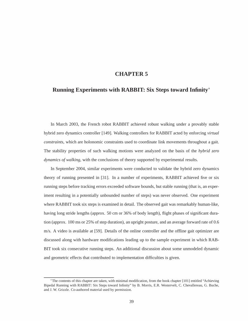
CHAPTER 5

Running Experiments with RABBIT: Six Steps toward Infinity ∗

In March 2003, the French robot RABBIT achieved robust walking under a provably stable

hybrid zero dynamics controller [149]. Walking controllers for RABBIT acted by enforcingvirtual

constraints, which are holonomic constraints used to coordinate link movements throughout a gait.

The stability properties of such walking motions were analyzed on the basis of thehybrid zero

dynamics of walking, with the conclusions of theory supported by experimental results.

In September 2004, similar experiments were conducted to validate the hybrid zero dynamics

theory of running presented in [31]. In a number of experiments, RABBIT achieved five or six

running steps before tracking errors exceeded software bounds, but stable running (that is, an exper-

iment resulting in a potentially unbounded number of steps)was never observed. One experiment

where RABBIT took six steps is examined in detail. The observed gait was remarkably human-like,

having long stride lengths (approx. 50 cm or 36% of body length), flight phases of significant dura-

tion (approx. 100 ms or 25% of step duration), an upright posture, and an average forward rate of 0.6

m/s. A video is available at [59]. Details of the online controller and the offline gait optimizer are

discussed along with hardware modifications leading up to the sample experiment in which RAB-

BIT took six consecutive running steps. An additional discussion about some unmodeled dynamic

and geometric effects that contributed to implementation difficulties is given.

∗The contents of this chapter are taken, with minimal modification, from the book chapter [101] entitled “AchievingBipedal Running with RABBIT: Six Steps toward Infinity” by B.Morris, E.R. Westervelt, C. Chevallereau, G. Buche,and J. W. Grizzle. Co-authored material used by permission.

39

(a) RABBIT

q1

q2

q3

q4

q5

(i) (ii) (iii)

xcm

ycm

y1

x1

y2

x2θs(q)

(b) Phases of running and coordinate conventions.

Figure 5.1: Phases of running and coordinate conventions. Astick figure of RABBIT is shown (i) at

the end of the stance phase with the stance leg in bold; (ii) during flight with the previous stance leg

in bold; and (iii) at the beginning of the stance phase just after landing and coordinate swap, with

the stance leg of the upcoming stance phase in bold. To avoid clutter, the coordinate conventions

have been spread out over the stance and flight phases. Anglesare positive in thecounterclockwise

direction.

The remainder of this chapter is a self-contained description of the theoretical development and

hardware modifications leading up to one example of an experiment in which RABBIT took six con-

secutive running steps. To facilitate implementation, thecontroller hypotheses of [31] are slightly

relaxed, leading to controllers that are easier to design than those proposed in [31] but which still

lend the closed-loop system to a reduced dimensionality stability test. Philosophy and motivation

of the modified control law are given in Section 5.1.1 with a detailed development of the hybrid

controller in Sections 5.1.3 to 5.1.7. The resulting closed-loop model of RABBIT and its stability

properties are discussed in Sections 5.1.8 and 5.1.9. Beyond this, Section 5.2 outlines a method for

the design of stable gaits using constrained nonlinear optimization and includes a numerical exam-

ple. Section 5.3 presents results from the first experimental implementation of running on RABBIT

and a discussion outlining a number of possible reasons why stable running was not observed. Con-

clusions are drawn in Section 5.4. Supplemental material not appearing in [101] is provided in

Section 5.5.

40

5.1 Controller Derivation

5.1.1 Summary and Philosophy

The overall philosophy of HZD control is to use the freedom available in feedback design

to achieve a parameterized family of closed-loop systems whose stability analysis is analytically

tractable. This allows the use of numerical optimization tosearch among the family of closed-loop

systems to find those that yield a desired behavior, such as stable running at a pre-determined speed

with upper bounds on peak actuator power and the coefficient of static friction between the leg end

and the ground.

Parameterization is achieved through the use of virtual constraints in both the stance and flight

phases. Perfect enforcement of virtual constraints results in low dimensional surfaces that are in-

variant under the differential equations of the closed-loop model and are also invariant under the

transition maps. To achieve the invariance at landing, a deadbeat action is incorporated in the flight

phase controller that steers the robot to land in a pre-determined configuration, while respecting

conservation of angular momentum about the robot’s center of mass. This hybrid controller creates

a 1DOF HZD that allows the stability of a running motion to be analyzed in closed form on the

basis of a one-dimensional Poincare map.

5.1.2 Parameterized Control with Impact Updated Parameters

In the first running experiment attempted on RABBIT, there was not sufficient time1 to imple-

ment completely the controller of [31]. The controller thatwas implemented used virtual constraints

in both the stance and flight phases, but the deadbeat action of the flight phase controller was not im-

plemented to regulate the final configuration of the robot at touchdown. Instead, to account for the

changing configuration of the robot at touchdown, the transition controller of [152] was adopted2.

Key points of the related analysis are highlighted in Section 5.1.9.

1A total of two weeks were available to perform the experiments.2The transition controller of this chapter takes into account the joint angles of the robot at touchdown but not the joint

angular velocities. As a result a true HZD of running is not created, and the resulting analysis of Section 5.1.9 (based on[60]) is modified accordingly.

41

5.1.3 Parameterized Virtual Constraints

For notational convenience, the stance phase and flight phase virtual constraints will be parame-

terized separately byas andaf , respectively. These parameter sets, which lie in the parameter spaces

As = IRns andAf = IRnf , can be updated at takeoff and landing events but are otherwise constant.

With this notation, the virtual constraints for stance and flight are, respectively,3

y = qb − hd,s(θs(qs), as) (5.1a)

y = qb − hd,f(θf(qf , af), af). (5.1b)

5.1.4 Stance Phase Control

The controller for the stance phase acts by updating the parametersas and by enforcing the

virtual constraints (5.1a). As a result of enforcing the virtual constraints, in stance phase, the robot

behaves as an unactuated 1 DOF system whose properties can betuned by choosing different con-

straint parameters. Apart from different boundary conditions on the virtual constraints, this control

is identical to the walking controllers developed in [153, 149]. The stance phase parameter vector,

as, can be expressed as

as = (as,0, as,1, . . . , as,ms−1, as,ms , θ−s , θ+s ), (5.2)

wherems ≥ 3, as,i ∈ IR4 for i ∈ {0, 1, . . . ,ms − 1,ms}, andθ−s , θ+s ∈ IR. Note thatns =

4 (ms + 1) + 2. The termsθ−s andθ+s are the values of the functionθs(qs) evaluated at the end and

the beginning of the stance phase. In [153, 149],hd is expressed in terms of Bezier polynomials.

Here, a slightly different class of polynomials4 is used that satisfy the following:

hd,s(θ+s , as) = as,0

ddθs

hd,s(θ−s , as) = as,ms−1

ddθs

hd,s(θ+s , as) = as,1 hd,s(θ

−s , as) = as,ms .

(5.3)

The stance phase virtual constraints are imposed on the dynamics by using a controlus : Xs×As →

IR4 that drives (5.1a) to zeroin finite time. The specific assumptions are as in [60, 153].

3Terms that are constant during the continuous phases of motion, and potentially updated at phase transitions, will beconsideredparameters.

4Any class of smooth functions satisfying these properties can be used to define virtual constraints.

42

5.1.5 Flight Phase Control

The development of the flight phase controller is similar to that of the stance phase controller.

The key difference is the choice ofθf in (5.1b) to be a function of the position of the center of mass.

The flight phase parameter vector,af , is defined as

af = (af,0, af,1, . . . , af,mf−1, af,mf, x+

cm,f , x+cm,f , Tf), (5.4)

wheremf ≥ 3, af,i ∈ IR4 for i ∈ {0, 1, . . . ,mf − 1,mf}, andx+cm,f , x

+cm,f , Tf ∈ IR. Note that

nf = 4 (mf + 1) + 3. The termsx+cm,f , x+

cm,f , andTf are, respectively, the horizontal position of

the center of mass at the beginning of the flight phase, the horizontal velocity of the center of mass

at the beginning of the flight phase, and the estimated5 duration of the flight phase. The flight phase

virtual constraints (5.1b) are given by

θf(qf , af) =1

Tf

(

xcm − x+cm,f

x+cm,f

)

, (5.5)

andhd,f , which, as in the stance phase, is a smooth, vector-valued function that satisfies

hd,f(0, af ) = af,0d

dθfhd,f(1, af) = af,mf−1

ddθf

hd,f(0, af ) = af,1 hd,f(1, af) = af,mf.

(5.6)

For a given stride, lettf denote the elapsed time within the flight phase. By conservation of linear

momentum,x+cm,f is constant during flight, which implies thattf = (xcm − x+

cm,f)/x+cm,f . As a

result,θf = tf/Tf is a valid substitute for (5.5), and for this reason, the given flight phase virtual

constraints are said to betime scaled. Flight phase virtual constraints are enforced using any smooth

state feedback controlleruf : Xf ×Af → IR4 that drives (5.1b) to zero exponentially quickly.

Note that finite time convergence is not used in the flight phase. A finite time controller is used

in the stance phase to render the stance phase constraint surface finite time attractive so that the

analysis of running will be similar to that of walking [60]. For further discussion of this point, refer

to Section 5.1.9.5Calculation ofTf requires the height of the center of mass at landing,y−

cm,f , to be knowna priori, which is onlypossible if the virtual constraints are exactly enforced throughout the flight phase.

43

5.1.6 Transition Control: Landing

In the event that landing occurs with the state of the robot not satisfying the virtual constraints,

the control parameters of the subsequent stance phase,as, are updated to ensure that the config-

uration of the robot satisfiesqb − hd,s(θ+s , as) = 0.6 The parameter updates are governed by the

differentiable functionw(f→s) : S(f→s) → As, such that foras = w(f→s)(x−f ),

as,0 = q+b

as,1 = a∗s,1

...

as,ms−1 = a∗s,ms−1

as,ms = a∗s,ms.

θ+s = θs(q

+s )

θ−s = θ−∗s

(5.7)

In the above,q+s is calculated using∆(f→s)(x

−f ), and the termsθ−∗

s anda∗s,i ∈ IR4, i ∈ {1, . . . ,ms−

1,ms} are constant parameters chosen during design.

If the stance phase finite time controller can satisfy the virtual constraints (5.1a) before the

liftoff event occurs, and the parameter updates obey (5.7),then the stance phase will terminate with

qb − hd,s(θ−s , as) = 0, or equivalently, withq− = q−∗.

5.1.7 Transition Control: Takeoff

At takeoff, the parameters of the flight phase virtual constraints, af , are updated so that the

duration of the planned motion of the robot is equal to the estimated flight time. Parameter up-

dates are governed by a continuously differentiable function w(s→f) : S(s→f) → Af , such that for

af = w(s→f)(x−s ),

6Our velocity estimates were rather noisy, so we did not update as,1. Updatingas,0 andas,1 would allow that justafter landing, the full state satisfied the virtual constraints.

44

af,0 = a∗f,0

af,1 = a∗f,1

...

af,mf−1 = a∗f,mf−1

af,mf= a∗f,mf

xcm+f = Υxcm(q−s )

x+cm,f =

∂Υxcm

∂qs(q−s ) q−s

Tf =y+cm,f

g+

√

(y+cm,f)

2 − 2g(y−∗cm,f − y+

cm,f)

g.

(5.8)

where,g is the magnitude of the acceleration of gravity andy−∗cm,f is the height of the center of

mass at the end of the flight phase, on the limit cycle. The terms a∗f,i ∈ IR4, i ∈ {0, 1, . . . ,mf −

1,mf} are parameters chosen during design. Initiation of the takeoff event is a control decision,

designated to occur whenθs(q) = θ−s . In the closed-loop model the switching hypersurface is

S(s→f) = {(xs, as) ∈ Xs ×As | H(s→f)(xs, as) = 0} whereH(s→f)(xs, as) = θs(qs) − θ−s .

5.1.8 Resulting Closed-Loop Model of Running

To form the closed-loop model of running, the state space of the open-loop model, (4.4), is

enlarged to include the parameters of the flight and stance phases. Define the augmented state

spaces

Xfe = Xf ×Af

Xse = Xs ×As

with elements given by

xfe = (qf , qf , af)

xse = (qs, qs, as).

The closed-loop dynamics can then be written as

ffe(xfe) =

ff(xf) + gf(xf)u(xf , af)

0Nf×1

fse(xse) =

fs(xs) + gs(xs)u(xs, as)

0Ns×1

.

45

The zero vectors reflect that the virtual constraint parameters do not change during the continuous

phases of running. The closed-loop impact maps include the parameter update laws,

∆(f→s)e(x−

fe) =

∆(f→s)(x−f )

w(f→s)(x−f )

∆(s→f)e(x−

se) =

∆(s→f)(x−s )

w(s→f)(x−s )

.

The closed-loop hybrid model is then

Σfe :

xfe = ffe(xfe) x−fe 6∈ S(f→s)e

x+se = ∆(f→s)e

(xfe) x−fe ∈ S(f→s)e

(5.9a)

Σse :

xse = fse(xse) x−se 6∈ S(s→f)e

x+fe = ∆(s→f)e

(xse) x−se ∈ S(s→f)e

,

(5.9b)

which may be written as

Σfe =(

Xfe,S(f→s)e,∆(f→s)e

, ffe

)

Σse =(

Xse,S(s→f)e,∆(s→f)e

, fse

)

.

5.1.9 Existence and Stability of Periodic Orbits

The first step to evaluate the stability of a running gait using the method of Poincare is to

construct a system with impulse effects (that is, a single-chart hybrid model) that has the same

Poincare map as (5.9). Following [31, Eq. (62)], define

Σ :

˙x = f(x) x− 6∈ S

x+ = ∆(x−) x− ∈ S,

where x = xse, f = fse, ∆ = ∆(f→s)e◦ φTI ,f ◦ ∆(s→f)e

, and S = S(s→f)e. In words, this

system consists of the differential equation of the closed-loop stance phase model of (5.9) and a

generalized impact map∆ that includes the transition map from stance to flight, the flight phase

dynamics, and the impact map from flight to stance. The generalized impact map is the result of

event-based sampling of the solution of (5.9) at takeoff events.

Because the virtual constraints in the stance phase are enforced using a continuous finite time

controller [17], the reduction technique of [60, Thm. 2] is applicable. Because the parameter updates

46

in the stance phase can be computed in terms of the state of therobot at takeoff, the analysis of

periodic orbits can be reduced to the computation of a one-dimensional restricted Poincare map,ρ,

havingS(s→f)eas a Poincare section.

5.2 Design of Running Motions with Optimization

5.2.1 Optimization Parameters

To design a running motion, a numerical routine is used to search the parameter spacesAs

andAf for a set of parameters that results in a desirable gait (periodic orbit of (5.9)). Common

requirements on the gait are achieved by incorporating constraints into the numerical search. Such

constraints address actuator limits, allowable joint space, and unilateral ground contact forces. For

the experiments reported here, the gait was designed using an optimization approach that combined

the ideas of [30] and [153]; the optimization was performed directly on the parameters of the virtual

constraints in order tosimultaneouslydetermine a periodic running motion and a controller that

achieves it. This is in contrast with the approach of [31] where virtual constraints are designed by

regression against optimal, pre-computed, periodic trajectories.

Virtual constraints are assumed to be satisfied on the periodic orbit, which has two conse-

quences: first, the integration of the closed-loop system dynamics can be performed using the

stance and flight phase zero dynamics (see [31] for details),resulting in short computation times;

and second, the virtual constraint parameters,as andaf , are not independent. Once the independent

parameters have been identified, standard numerical optimization routines can be used to search for

desirable gaits. The implementation of such a procedure is outlined in the following subsections.

5.2.2 Boundary Conditions of the Virtual Constraints

The transition maps of takeoff and landing can be used to identify redundancies between the

virtual constraint parameter vectorsas andaf . Given the state corresponding to the end of the limit

cycle stance phase,x−∗s = (q−∗

s , q−∗s ), the state at the beginning of the subsequent flight phase can

be computed asx+∗f = (q+∗

f , q+∗f ) = ∆(s→f)(x

−∗s ). For bothx−∗

s and x+∗f to satisfy the virtual

47

constraints of their respective phases, the following relations must hold,

a∗s,ms−1 = q−∗b,s /θ−∗

s a∗f,0 = q+∗b,f

a∗s,ms= q−∗

b,s a∗f,1 = q+∗b,f T ∗

f ,

(5.10)

which are derived by applying (5.3), (5.5), (5.6), and (5.8)to (5.1). These are the boundary condi-

tions associated with the liftoff event of the periodic orbit. The state of the robot at the beginning

of the stance phase,x+∗s = (q+∗

s , q+∗s ), can be related to the state at the end of the previous flight

phase,x−∗f = (q−∗

f , q−∗f ), by the landing map,x+∗

s = ∆(f→s)(x−∗f ), to yield the following addi-

tional design constraints,

a∗s,0 = q+∗b,s a∗f,mf−1 = q−∗

b,f T ∗f

a∗s,1 = q+∗b,s /θ+∗

s a∗f,mf= q−∗

b,f .

(5.11)

The update law presented here enforces fewer boundary conditions than the update law of [31].

The extra boundary conditions associated with takeoff are already satisfied by (5.10), but those

of landing are not met by (5.11); they are more difficult to satisfy due to conservation of angular

momentum in the flight phase. The main theoretical result of this chapter is that invariance of the

flight and stance phase constraint surfaces over the landingevent is not a necessary condition for

achieving provably stable running. As noted earlier, relaxing this condition makes running motions

significantly easier to design.

5.2.3 Optimization Algorithm Details

Trial gaits for the running experiments were generated using the constrained nonlinear opti-

mization routinefmincon of MATLAB’s Optimization Toolbox. Three quantities are involved in

optimization:J, a scalar cost function to be minimized on the periodic orbit, EQ, a vector of equality

constraints, andINEQ, a vector of inequality constraints. The following is a description of the op-

timization procedure that was implemented. The independent and dependent terms7 of optimization

are given in Table 5.1. Note that when the optimizer terminates with the constraints satisfied,x+∗s

will be a point located on a closed-loop periodic orbit and the virtual constraints will be given by

(5.2) and (5.4).7“Terms” is used to describe those variables used in optimization; these are different from the “parameters” of the

virtual constraints.

48

Algorithm

1. Selectx−∗f = (q−∗

f , q−∗f ), the state corresponding to the end of the flight phase.

2. Using the flight-to-stance transition function,∆(f→s), calculatex+∗s = (q+∗

s , q+∗s ), the state

corresponding to the beginning of the subsequent stance phase.

3. Calculateθ+∗s by (5.7) anda∗s,0, a∗s,1 by (5.11).

4. Selecta∗s,2, . . . , a∗s,ms

, andθ−∗s to complete the stance phase parameter vectoras.

5. Using parametersas and the initial conditionx+∗s , integrate the equations of motion of stance

and apply the stance-to-flight transition operator,∆(s→f), to obtainx+∗f = (q+∗

f , q+∗f ).

6. Calculatea∗f,0, a∗f,1 by (5.10);a∗f,mf−1, a∗f,mfby (5.11); andx+∗

cm,f , x+∗cm,f , andT ∗

f by (5.8).

7. Selecta∗f,2, . . . , a∗f,mf−2 to complete the flight phase parameter vectoraf .

8. Using parametersaf , and initial conditionx+∗f , integrate the equations of motion of flight to

obtainx−f .

9. EvaluateJ, EQ, andINEQ.

10. Iterate Steps 1 to 9 untilJ is (approximately) minimized, each entry ofEQ is zero, and each

entry ofINEQ is less than zero.

5.2.4 An Example Running Motion

A sample running gait designed by the above algorithm is now presented. A stick diagram of

this motion is given in Figure 5.2(a). The stability analysis outlined in Section 5.1.9 was applied to

the resulting running motion. Figure 5.2(b) gives the restricted Poincare map, which indicates that

the motion is locally exponentially stable. The gait was designed to minimize the integral of torque

squared per distance traveled, with the following constraints:

Equality constraints, EQ

• error associated with finding a fixed point||x−f − x−∗

f ||

49

Terms of Optimization

Independent Dependent

x−∗f ∈ IR14 θ+∗

s ∈ IR

a∗s,2, . . . , a∗s,ms

∈ IR4 a∗s,0, a∗s,1 ∈ IR4

θ−∗s ∈ IR x+∗

s ∈ IR10

a∗f,2, . . . , a∗f,mf−2 ∈ IR4 a∗f,0, a∗f,1 ∈ IR4

a∗f,mf−1, a∗f,mf∈ IR4

x+∗cm,f , x+∗

cm,f , T ∗f ∈ IR

x−f ∈ IR14

Table 5.1: Independent and dependent terms used in optimization. The choice of the independent

terms is non-unique and depends on the specific optimizationprocedure. The parameters below

correspond to the algorithm in Section 5.2.3, which is one straightforward method to ensure the

boundary conditions of the virtual constraints are met.

• deviation from the desired running rate

• required frictional forces at the leg ends are zero just before takeoff and just after landing (to

prevent slipping at these transitions)

Inequality constraints, INEQ

• magnitude of the required torque at each joint less than 100 Nm

• knee angles to lie in(0◦,−70◦) and hip angles to lie in(130◦, 250◦) (see Figure 5.1(b) for

measurement conventions)

• minimum height of the swing foot during stance greater than 7cm

• required coefficient of friction of the stance phase less than 0.7

• flight time greater than or equal to 25% of total gait duration

• landing foot impacts the ground at an angle of approach less than45◦ from vertical

• joint angular velocities less than 5 rad/s

50

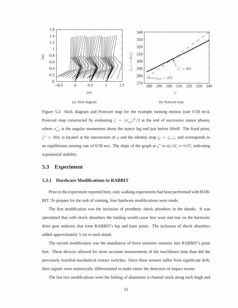
−0.5 0 0.5 1 1.5

0.4

0.6

1.2

0.2

0.8

1.4

1.6

0

1

(m)

(m)

(a) Stick diagram

280 290 300 310 320 330 340270

280

290

300

310

320

330

340

ζi

ζ i+

1=

ρ(ζ

i)

ζmin = 275

ζ∗ = 303

(b) Poincare map

Figure 5.2: Stick diagram and Poincare map for the example running motion (rate 0.58 m/s).

Poincare map constructed by evaluatingζ = (σ−s,1)

2/2 at the end of successive stance phases,

whereσ−s,1 is the angular momentum about the stance leg end just before liftoff. The fixed point,

ζ∗ = 303, is located at the intersection ofρ and the identity mapζi = ζi+1, and corresponds to

an equilibrium running rate of 0.58 m/s. The slope of the graph atζ∗ is dρ/dζ ≈ 0.67, indicating

exponential stability.

5.3 Experiment

5.3.1 Hardware Modifications to RABBIT

Prior to the experiment reported here, only walking experiments had been performed with RAB-

BIT. To prepare for the task of running, four hardware modifications were made.

The first modification was the inclusion of prosthetic shock absorbers in the shanks. It was

speculated that with shock absorbers the landing would cause less wear and tear on the harmonic

drive gear reducers that form RABBIT’s hip and knee joints. The inclusion of shock absorbers

added approximately 5 cm to each shank.

The second modification was the installation of force sensitive resistors into RABBIT’s point

feet. These devices allowed for more accurate measurement of the touchdown time than did the

previously installed mechanical contact switches. Since these sensors suffer from significant drift,

their signals were numerically differentiated to make easier the detection of impact events.

The last two modifications were the bolting of aluminum u-channel stock along each thigh and

51

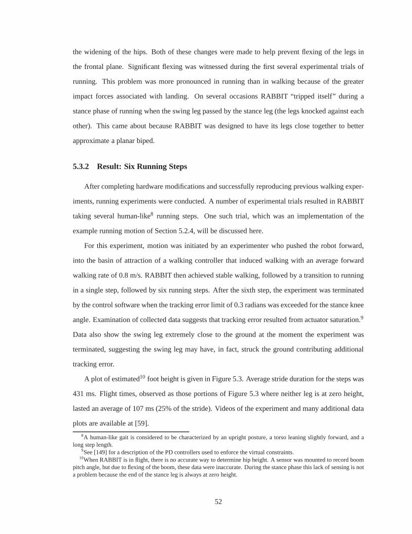
the widening of the hips. Both of these changes were made to help prevent flexing of the legs in

the frontal plane. Significant flexing was witnessed during the first several experimental trials of

running. This problem was more pronounced in running than inwalking because of the greater

impact forces associated with landing. On several occasions RABBIT “tripped itself” during a

stance phase of running when the swing leg passed by the stance leg (the legs knocked against each

other). This came about because RABBIT was designed to have its legs close together to better

approximate a planar biped.

5.3.2 Result: Six Running Steps

After completing hardware modifications and successfully reproducing previous walking exper-

iments, running experiments were conducted. A number of experimental trials resulted in RABBIT

taking several human-like8 running steps. One such trial, which was an implementation of the

example running motion of Section 5.2.4, will be discussed here.

For this experiment, motion was initiated by an experimenter who pushed the robot forward,

into the basin of attraction of a walking controller that induced walking with an average forward

walking rate of 0.8 m/s. RABBIT then achieved stable walking, followed by a transition to running

in a single step, followed by six running steps. After the sixth step, the experiment was terminated

by the control software when the tracking error limit of 0.3 radians was exceeded for the stance knee

angle. Examination of collected data suggests that tracking error resulted from actuator saturation.9

Data also show the swing leg extremely close to the ground at the moment the experiment was

terminated, suggesting the swing leg may have, in fact, struck the ground contributing additional

tracking error.

A plot of estimated10 foot height is given in Figure 5.3. Average stride duration for the steps was

431 ms. Flight times, observed as those portions of Figure 5.3 where neither leg is at zero height,

lasted an average of 107 ms (25% of the stride). Videos of the experiment and many additional data

plots are available at [59].

8A human-like gait is considered to be characterized by an upright posture, a torso leaning slightly forward, and along step length.

9See [149] for a description of the PD controllers used to enforce the virtual constraints.10When RABBIT is in flight, there is no accurate way to determinehip height. A sensor was mounted to record boom

pitch angle, but due to flexing of the boom, these data were inaccurate. During the stance phase this lack of sensing is nota problem because the end of the stance leg is always at zero height.

52

18.5 19 19.5 20 20.5 21 21.5

0.16

0.12

0.08

0.04

0es

timat

edhe

ight

(m)

time (sec)

Figure 5.3: Estimated height of RABBIT’s point feet during the reported running experiment. RAB-

BIT’s left foot is indicated in bold. Flight phases occur when neither foot is at zero height.

Several problematic issues related to RABBIT’s hardware did not appear until running was

attempted. (For a discussion of general implementation issues of walking including unmodeled

effects of the boom, gear reducers, and an uneven walking surface see [149].) Future running

experiments—whether on RABBIT or another, similar mechanism—should take into account the

following issues.

Boom dynamics

The perturbing effects of the boom were found to be much more significant during flight phases

than during stance phases. When RABBIT is modeled as a planarsystem, an analysis of the three-

dimensional mechanics shows that the contribution of the boom to the center of mass dynamics is

significant. Specifically,q5 is no longer, in general, a cyclic variable during flight. However, if boom

masses are appropriately distributed, the parabolic motion of the center of mass, as modeled in a

planar system, is recovered. Unfortunately, this special mass distribution was impossible because

RABBIT does not have a counterweight system.

Walking surface

The walking surface was also a source of problems. This surface—consisting of rubber over el-

evated plywood supported on the edges by a wood frame—was originally built to provide a uniform,

level surface. Although the surface appears uniform, walking experiments demonstrated otherwise.

It was found that the surface has “fast” and “slow” areas corresponding to varying floor stiffness

53

and coefficient of friction.

Limited joint space

For safety, RABBIT’s joints have hard stops that limit its joint space, which, for example, pre-

vent the shank from contacting the thigh. Although the available joint space was sufficient for

walking, it became a significantly limiting factor in the design of running gaits. These hard stops

prevented the swing leg from being folded close to the hip, which is a natural and desirable motion

that minimizes the leg’s rotational inertia.

5.4 Conclusion

A novel approach to the control of running in planar bipeds and its first experimental imple-

mentation on RABBIT have been presented. The control law is hybrid, consisting of continuous

actions in the stance and flight phases and discrete actions at the transitions between these phases.

In the stance and flight phases, the controller coordinates the relative motions of the robot’s links by

imposing virtual constraints at the actuated joints. At thetransition from stance to flight, the con-

troller adjusts the virtual constraints for the flight phaseas a function of estimated flight duration

to ensure that the former swing leg is advanced properly to take up its role as the next stance leg.

At the transition from flight to stance, the controller updates the virtual constraints of the stance

phase to account for the orientation of the robot at landing.For the nominal periodic running mo-

tion, the parameters of the virtual constraints are determined by numerical optimization in order to

meet actuator power limits, friction bounds, joint limits,etc. For running experiments, RABBIT’s

mechanical and electrical systems were modified: shock absorbers were added to the shanks; the

ground contact sensors were improved; the stiffnesses of legs in the frontal plane were increased;

and the hips were widened.

The main theoretical result of this chapter was the development of a running controller that

is based on the HZD methodology, but easier to design and implement while still resulting in a

reduced dimensionality stability test. The main experimental result of this chapter was the physical

realization of six consecutive running steps with a human-like gait and identification of hardware

difficulties of running with RABBIT that were not present in walking.

54

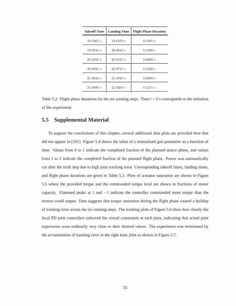
Takeoff Time Landing Time Flight Phase Duration

19.5465 s 19.6470 s 0.1005 s

19.9545 s 20.0835 s 0.1290 s

20.4255 s 20.5215 s 0.0960 s

20.8695 s 20.9715 s 0.1020 s

21.3045 s 21.3945 s 0.0900 s

21.6990 s 21.8205 s 0.1215 s

Table 5.2: Flight phase durations for the six running steps.Timet = 0 s corresponds to the initiation

of the experiment.

5.5 Supplemental Material

To support the conclusions of this chapter, several additional data plots are provided here that

did not appear in [101]. Figure 5.4 shows the value of a normalized gait parameter as a function of

time. Values from 0 to 1 indicate the completed fraction of the planned stance phase, and values

from 1 to 2 indicate the completed fraction of the planned flight phase. Power was automatically

cut after the sixth step due to high joint tracking error. Corresponding takeoff times, landing times,

and flight phase durations are given in Table 5.2. Plots of actuator saturation are shown in Figure

5.5 where the provided torque and the commanded torque levelare shown in fractions of motor

capacity. Flattened peaks at1 and−1 indicate the controller commanded more torque than the

motors could output. Data suggests that torque saturation during the flight phase caused a buildup

of tracking error across the six running steps. The trackingplots of Figure 5.6 show how closely the

local PD joint controllers enforced the virtual constraints at each joint, indicating that actual joint

trajectories were ordinarily very close to their desired values. The experiment was terminated by

the accumulation of tracking error in the right knee joint asshown in Figure 5.7.

55

18.5 19 19.5 20 20.5 21 21.5 220

0.5

1

1.5

2

time (s)

norm

aliz

ed g

ait p

aram

eter

Figure 5.4: Normalized gait parameter showing the existence of six running steps. Values from 0

to 1 indicate the completed fraction of the planned stance phase, and values from 1 to 2 indicate the

completed fraction of the planned flight phase.

56

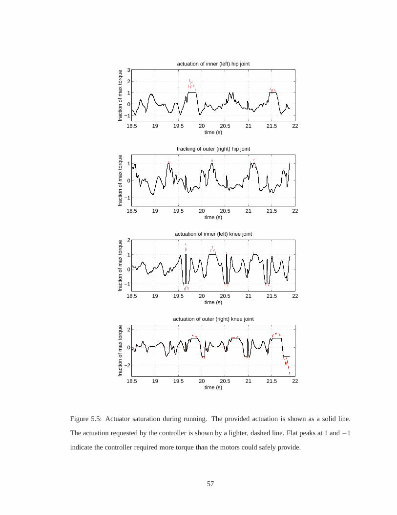
18.5 19 19.5 20 20.5 21 21.5 22

−1

0

1

2

3actuation of inner (left) hip joint

time (s)

frac

tion

of m

ax to

rque

18.5 19 19.5 20 20.5 21 21.5 22

−1

0

1

tracking of outer (right) hip joint

time (s)

frac

tion

of m

ax to

rque

18.5 19 19.5 20 20.5 21 21.5 22

−1

0

1

2actuation of inner (left) knee joint

time (s)

frac

tion

of m

ax to

rque

18.5 19 19.5 20 20.5 21 21.5 22

−2

0

2

actuation of outer (right) knee joint

time (s)

frac

tion

of m

ax to

rque

Figure 5.5: Actuator saturation during running. The provided actuation is shown as a solid line.

The actuation requested by the controller is shown by a lighter, dashed line. Flat peaks at1 and−1

indicate the controller required more torque than the motors could safely provide.

57

18.5 19 19.5 20 20.5 21 21.5 22

3

3.5

4

tracking of inner (left) hip joint

time (s)

rad

18.5 19 19.5 20 20.5 21 21.5 22

3

3.5

4

tracking of outer (right) hip joint

time (s)

rad

18.5 19 19.5 20 20.5 21 21.5 22

−1.2

−1

−0.8

−0.6

−0.4

tracking of inner (left) knee joint

time (s)

rad

18.5 19 19.5 20 20.5 21 21.5 22

−1.2

−1

−0.8

−0.6

−0.4

tracking of outer (right) knee joint

rad

time (s)

Figure 5.6: Joint tracking performance during running. Theobserved trajectory is shown as a solid

line, the reference trajectory, by a lighter, dashed line.

58

18.5 19 19.5 20 20.5 21 21.5 22

−0.1

0

0.1

tracking error of inner (left) hip joint

rad

time (s)

18.5 19 19.5 20 20.5 21 21.5 22−0.1

−0.05

0

0.05

tracking error of outer (right) hip joint

rad

time (s)

18.5 19 19.5 20 20.5 21 21.5 22

−0.1

0

0.1

tracking error of inner (left) knee joint

rad

time (s)

18.5 19 19.5 20 20.5 21 21.5 22−0.2

0

0.2

tracking error of outer (right) knee joint

rad

time (s)

Figure 5.7: Joint tracking error during running. An accumulation of error in the outer knee triggered

safety conditions that automatically terminated the experiment.

59

Notation Introduced in Chapter 5

Symbol Meaning Defined

As parameter space of the virtual constraints of stance Section 5.1.3

Af parameter space of the virtual constraints of flight Section 5.1.3

hd,s, θs functions defining the virtual constraints of stance Section 5.1.3

hd,f , θf functions defining the virtual constraints of flight Section 5.1.3

w(f→s) parameter updates at landing Section 5.1.6

w(s→f) parameter updates at liftoff Section 5.1.7

Xse state manifold of the closed-loop stance phase Section 5.1.8

Xfe state manifold of the closed-loop flight phase Section 5.1.8

xse state of the robot in closed-loop stance Section 5.1.8

xfe state of the robot in closed-loop flight Section 5.1.8

fse vector field of the closed-loop stance phase Section 5.1.8

ffe vector field of the closed-loop flight phase Section 5.1.8

∆(s→f)e

closed-loop liftoff map Section 5.1.8

∆(f→s)e

closed-loop landing map Section 5.1.8

Σse model of the closed-loop stance phase Section 5.1.8

Σfe model of the closed-loop flight phase Section 5.1.8

60

CHAPTER 6

Sample-Based HZD Control for Robustness and Slope Invariance of

Planar Passive Bipedal Gaits∗

To explore potential connections between passive dynamic walkers and hybrid zero dynamics

controllers, this chapter presents new analysis results and tools for the HZD framework. These in-

clude (i) analysis of the effects of walking on a slope, (ii) analysis of dynamic singularities resulting

from enforcing virtual constraints, and (iii) an alternative method for designing virtual constraints.

Extensions are motivated by a desire to make the gaits of passive walkers robust to disturbances.

As noted in Chapter 2, passive bipedal walkers have the ability to walk stably down a slope without

the use of actuation [96] and typically suffer from sensitivity to initial conditions and to external

disturbances. The new results and tools facilitate the design of controllers to make such passive

gaits robust.

The first result, analysis of walking on a slope, is an extension of [153, 149] in which compo-

nents of the closed-loop system dynamics are examined to determine the overall effects of changing

ground slope. Results make indirect use of observations given in [133] regarding the fact that planar

rotations of the robot are a group symmetry of the robot’s kinetic energy but not of its potential

energy.

The second result sheds light onto the condition of decoupling matrix invertibility. For an HZD

controller to be valid, the decoupling matrix associated with performing input-output linearization of

∗The contents of this chapter are taken, with minimal modification, from the journal article [154] entitled “AnalysisResults and Tools for the Control of Planar Bipedal Gaits using Hybrid Zero Dynamics” by E. R. Westervelt, B. Morris,and K. D. Farrell. Co-authored material used by permission.

61

the robot’s dynamics must be invertible [78, Chp. 5]. The closed-loop system is said to encounter a

dynamic singularityat points where the decoupling matrix is noninvertible. This definition is used to

parallel the notion of a kinematic singularity1. Dynamic singularities, like kinematic singularities,

represent configurations of the robot at which there is a reduction in the number of DOFs. But,

unlike kinematic singularities—which arise from the mechanism’s kinematics and involve only its

kinematic parameters—dynamic singularities involve bothkinematic and inertial parameters. One

type of dynamic singularity related to bipedal walking involves the decoupling matrix used in HZD

feedback controllers. Other types of dynamic singularities will not be considered. It is shown that

decoupling matrix singularities can be computed with a relatively simple, closed form expression.

Interpretations of dynamic singularities are given as wellas analysis of the effects of approaching a

singularity.

The third result, an alternative method for designing virtual constraints, expands the set of refer-

ence gaits controllable within the HZD framework, separating gait design and controller design into

two distinct steps. In previous work, the virtual constraints were chosen using numerical optimiza-

tion over a pre-chosen, finitely parameterized family of constraints. This technique is acceptable

when the objective of controller design is to find a gait with certain stability and energetic proper-

ties. However, when the goal is to exactly achieve a given gait, existing techniques can do no better

than to project the motion onto the closest member of the parameterized family of constraints. The

alternative method, termedsample-based HZD control, does not use a pre-chosen family of virtual

constraints. In essence, a given (period-one) gait is sampled to obtain full state information at cho-

sen instants of time. Certain normalized quantities are computed from this full state information

and are used to define the virtual constraints of an HZD controller. The sampled gait can be ob-

tained from, for example, a gait induced by a potentially unknown control strategy, or a gait whose

corresponding control strategy is not equivalent to imposing holonomic constraints. An example

of the latter is the work of [30] where joint motions were designed to be polynomial functions of

time, rather than of state. By using this approach, it is usually not possible toexplicitly represent the

motions as following holonomic constraints [28].2

With regard to passive gaits, sample-based HZD control enables the design of controllers that

1For other definitions of dynamic singularities relating to spacecraft manipulators, see [105, 158].2What this section provides is a computationally tractableimplicit representation of the holonomic constraints that

correspond to such motions.

62

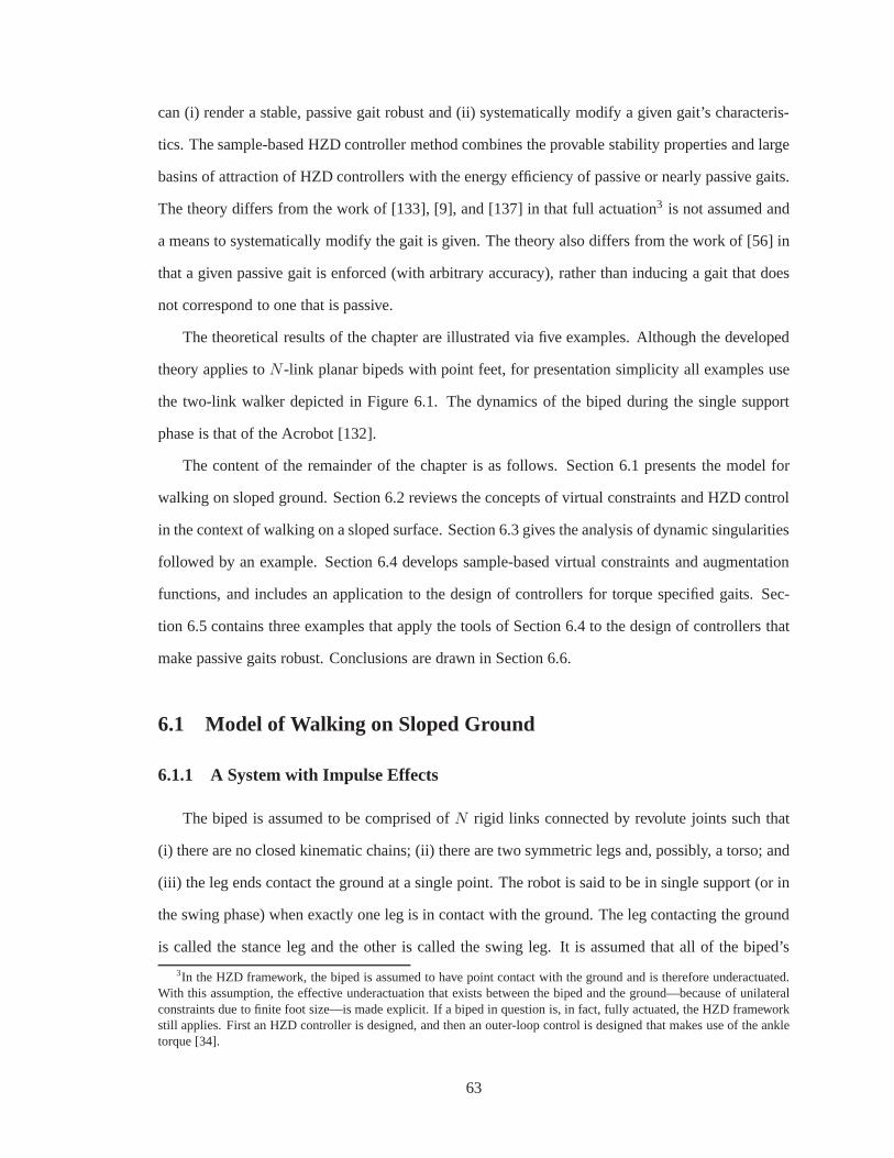
can (i) render a stable, passive gait robust and (ii) systematically modify a given gait’s characteris-

tics. The sample-based HZD controller method combines the provable stability properties and large

basins of attraction of HZD controllers with the energy efficiency of passive or nearly passive gaits.

The theory differs from the work of [133], [9], and [137] in that full actuation3 is not assumed and

a means to systematically modify the gait is given. The theory also differs from the work of [56] in

that a given passive gait is enforced (with arbitrary accuracy), rather than inducing a gait that does

not correspond to one that is passive.

The theoretical results of the chapter are illustrated via five examples. Although the developed

theory applies toN -link planar bipeds with point feet, for presentation simplicity all examples use

the two-link walker depicted in Figure 6.1. The dynamics of the biped during the single support

phase is that of the Acrobot [132].

The content of the remainder of the chapter is as follows. Section 6.1 presents the model for

walking on sloped ground. Section 6.2 reviews the concepts of virtual constraints and HZD control

in the context of walking on a sloped surface. Section 6.3 gives the analysis of dynamic singularities

followed by an example. Section 6.4 develops sample-based virtual constraints and augmentation

functions, and includes an application to the design of controllers for torque specified gaits. Sec-

tion 6.5 contains three examples that apply the tools of Section 6.4 to the design of controllers that

make passive gaits robust. Conclusions are drawn in Section6.6.

6.1 Model of Walking on Sloped Ground

6.1.1 A System with Impulse Effects

The biped is assumed to be comprised ofN rigid links connected by revolute joints such that

(i) there are no closed kinematic chains; (ii) there are two symmetric legs and, possibly, a torso; and

(iii) the leg ends contact the ground at a single point. The robot is said to be in single support (or in

the swing phase) when exactly one leg is in contact with the ground. The leg contacting the ground

is called the stance leg and the other is called the swing leg.It is assumed that all of the biped’s

3In the HZD framework, the biped is assumed to have point contact with the ground and is therefore underactuated.With this assumption, the effective underactuation that exists between the biped and the ground—because of unilateralconstraints due to finite foot size—is made explicit. If a biped in question is, in fact, fully actuated, the HZD frameworkstill applies. First an HZD controller is designed, and thenan outer-loop control is designed that makes use of the ankletorque [34].

63

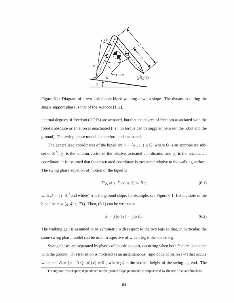
α

(ph2 ,pv

2)

x

y

q1

q2

lcl

COM

Figure 6.1: Diagram of a two-link planar biped walking down aslope. The dynamics during the

single support phase is that of the Acrobot [132].

internal degrees of freedom (DOFs) are actuated, but that the degree of freedom associated with the

robot’s absolute orientation is unactuated (i.e., no torque can be supplied between the robot and the

ground). The swing phase model is therefore underactuated.

The generalized coordinates of the biped areq = (qa, qu) ∈ Q, whereQ is an appropriate sub-

set ofRN , qa is the column vector of the relative, actuated coordinates,andqu is the unactuated

coordinate. It is assumed that the unactuated coordinate ismeasured relative to the walking surface.

The swing phase equation of motion of the biped is

D(q)q + F [α](q, q) = Bu, (6.1)

with B = [ I 0 ]′ and where4 α is the ground slope; for example, see Figure 6.1. Let the state of the

biped bex = (q, q) ∈ TQ. Then, (6.1) can be written as

x = f [α](x) + g(x)u. (6.2)

The walking gait is assumed to be symmetric with respect to the two legs so that, in particular, the

same swing phase model can be used irrespective of which leg is the stance leg.

Swing phases are separated by phases of double support, occurring when both feet are in contact

with the ground. This transition is modeled as an instantaneous, rigid body collision [74] that occurs

whenx ∈ S = {x ∈ TQ | pv2(x) = 0}, wherepv

2 is the vertical height of the swing leg end. The

4Throughout this chapter, dependence on the ground slope parameter is emphasized by the use of square brackets.

64

transition model, which includes a permutation of the coordinates to account for the swapping of

the legs’ roles, is algebraic and can be written as

x+ = ∆(x−), (6.3)

where the superscript “+” (resp. “−”) refers to the value at the beginning (resp. end) of a step.

The overall model is expressed as a single-charted system with impulse effects:

Σ :

x = f [α](x) + g(x)u, x− 6∈ S

x+ = ∆(x−), x− ∈ S.

(6.4)

Walking gaits will be analyzed as periodic orbits of (6.4), with stability of a walking gait referring to

stability of the corresponding periodic orbit. For formal definitions of solutions, orbits, and stability

relating to (6.4), see [60].

6.1.2 Example Model: A Two-Link Walker

For presentation simplicity, the results of this chapter will be illustrated on a two-link biped

walker—a biped with the fewest number of links to which the results apply. The biped is depicted

in Figure 6.1, and its parameters are given in Table 6.1. The terms of the equations of motion for

the walker are as follows. The (symmetric) mass inertia matrix is

D11(q1) = (l − lc)2 m + J (6.5a)

D12(q1) = m l(l − lc) cos(q1) − (l − lc)2 m − J (6.5b)

D22(q1) = −2m l(l − lc) cos(q1) +(2(l2c + l2) − 2 lc l

)m + 2J. (6.5c)

The vector of Coriolis, centrifugal, and gravity terms is

F1[α](q, q) = −m l sin(q1)(l − lc)q22 + m g0 sin(q1 − q2 − α)(l − lc) (6.6a)

F2[α](q, q) = −m l sin(q1)(l − lc)(q1 − q2)q1 + m l sin(q1)(l − lc)q1q2

+ m g0

((lc − l) sin(q1 − q2 − α) − sin(q2 + α)(lc + l)

). (6.6b)

Leg scuffing that necessarily occurs during the swing phase of the two-link walker is ignored.

65

Parameter Units Value

Leg length,l m 1.0

Leg COM location,lc m 0.8

Leg mass,m kg 0.3

Leg inertia about leg COM,J kg·m2 0.03

Acceleration due to gravity,g0 m/s2 9.81

Table 6.1: Parameters of the two-link model. (Parameters taken from [48, Tab. 4.1].)

6.2 HZD Framework for the Control of Walking on Sloped Ground

6.2.1 Defining Virtual Constraints

Virtual constraints are holonomic constraints that are imposed on the robot’s configuration by

feedback. These constraints are parameterized by a scalar function of the robot’s configuration,

and, when enforced by feedback, effectively reduce the closed-loop DOFs of the robot. When

virtual constraints satisfying certain invariance properties are exactly enforced, the HZD of walking

results.

To formally define virtual constraints, consider the following output on (6.2),

θ(q) : Q → Rθ ⊂ R (6.7a)

s(θ) : Rθ → [ 0, 1 ] (6.7b)

hd(s) : [ 0, 1 ] → RN−1 (6.7c)

y = h(q) = qa − hd ◦ s ◦ θ(q) (6.7d)

whereθ(q) is a function that is monotonic over a step and has a compact imageRθ, s(θ) is a

bijection with respect toRθ and normalizesθ to the unit interval, andhd(s) is a twice continuously

differentiable function that gives the actuated coordinates of the robot. For notational simplicity,

definehd(θ) = hd ◦ s(θ) so that (6.7d) can be written

y = qa − hd ◦ θ(q) . (6.8)

Let θ+ andθ− denote, respectively, the values ofθ(q) at the beginning and the end of a step. Then,

66

a valid choice fors, is s(θ) = (θ − θ+)/(θ− − θ+) with

θ = c q, (6.9)

wherec = (c1, c2), c1 ∈ RN−1 andc2 ∈ R with c2 nonzero. This choice will be assumed for the

remainder of the chapter. Virtual constraints are said to besatisfied or enforced wheny ≡ 0. The

constraint surfaceZ is defined as the subset ofTQ where the virtual constraints are satisfied,

Z = {x ∈ TQ | h(x) = 0, Lfh(x) = 0}. (6.10)

Note that it can be easily verified thatLgh(x) = 0 for all x ∈ TQ.

When viewed within the context of the hybrid model (6.4), thevirtual constraints are required

to have two types of invariance: forward invariance (or continuous phase invariance) and impact in-

variance (or invariance across the impact event). Continuous phase invariance refers to the property

that once a solution of (6.4) is within the constraint surface, the solution remains in the constraint

surface until the end of the single support phase. This type of invariance is achieved by the appro-

priate design of a feedback controller. The virtual constraints are invariant across the impact event if

lying within the constraint surface before impact guarantees that the solution will lie within the con-

straint surface after impact. This type of invariance is a property of virtual constraints themselves

and is independent of the feedback controller.

6.2.2 A Feedback yielding Continuous Phase Invariance

Assume a constraint of the form (6.7), which may or may not be impact invariant. The controller

given in this subsection will render it continuous phase invariant. The controller’s development

begins by taking the first two derivatives of the constraint,

y = qa −∂hd(θ)

∂θθ, (6.11a)

y = Υ(θ) q −∂2hd(θ)

∂θ2θ2, (6.11b)

Υ(θ) =

[

H −∂hd(θ)

∂θc

]

, (6.12)

H =

[

I(N−1)×(N−1) 0(N−1)×1

]

. (6.13)

67

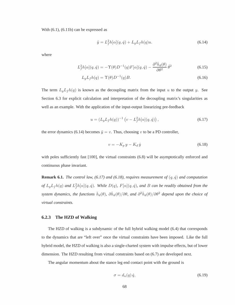
With (6.1), (6.11b) can be expressed as

y = L2fh[α](q, q) + LgLfh(q)u. (6.14)

where

L2fh[α](q, q) = −Υ(θ)D−1(q)F [α](q, q) −

∂2hd(θ)

∂θ2θ2 (6.15)

LgLfh(q) = Υ(θ)D−1(q)B. (6.16)

The termLgLfh(q) is known as the decoupling matrix from the inputu to the outputy. See

Section 6.3 for explicit calculation and interpretation ofthe decoupling matrix’s singularities as

well as an example. With the application of the input-outputlinearizing pre-feedback

u = (LgLfh(q))−1(v − L2

fh[α](q, q)), (6.17)

the error dynamics (6.14) becomesy = v. Thus, choosingv to be a PD controller,

v = −Kp y − Kd y (6.18)

with poles sufficiently fast [100], the virtual constraints(6.8) will be asymptotically enforced and

continuous phase invariant.

Remark 6.1. The control law, (6.17) and (6.18), requires measurement of(q, q) and computation

of LgLfh(q) and L2fh[α](q, q). WhileD(q), F [α](q, q), andB can be readily obtained from the

system dynamics, the functionshd(θ), ∂hd(θ)/∂θ, and ∂2hd(θ)/∂θ2 depend upon the choice of

virtual constraints.

6.2.3 The HZD of Walking

The HZD of walking is a subdynamic of the full hybrid walking model (6.4) that corresponds

to the dynamics that are “left over” once the virtual constraints have been imposed. Like the full

hybrid model, the HZD of walking is also a single-charted system with impulse effects, but of lower

dimension. The HZD resulting from virtual constraints based on (6.7) are developed next.

The angular momentum about the stance leg end contact point with the ground is

σ = dn(q) q, (6.19)

68

wheredn is the last row ofD. In a neighborhood of any point where the decoupling matrix is

invertible, (y, y, θ, σ) is a valid change of coordinates5 on TQ. Furthermore, the inverse of the

coordinate change is given by

q = Φq(θ, y) (6.20a)

q = Φq(θ, σ, y, y), (6.20b)

where

Φq(θ, y) =

H

c

−1

hd(θ) + y

θ

(6.21a)

Φq(θ, σ, y, y) =

Υ(θ)

dn(q)

−1∣∣∣∣∣∣∣∣q=Φq(θ,y)

y

σ

. (6.21b)

Assuming that the decoupling matrix is invertible, the zerodynamics manifold can be written as

Z =

(q, q) ∈ TQ

∣∣∣∣∣∣∣

q = Φq(θ, 0), q = Φq(θ, σ, 0, 0),

θ ∈ [θ+, θ−], σ ∈ R

. (6.22)

With the output given by (6.7), and a few additional technical assumptions (see [153, Thm. 1]), the

swing phase zero dynamics—the maximum dynamics that are compatible withy ≡ 0—are

θ =1

I(θ, 0)σ, (6.23a)

σ = Mt g0 xcm[α](θ, 0), (6.23b)

where

I(θ, y) = (cΦq(θ, 1, y, 0))−1 (6.24)

and whereMt is the total mass of the biped,g0 is the magnitude of the acceleration of gravity, and

xcm[α](θ, y) is the horizontal position of the center of mass measured with respect to the stance leg

end [29, Eq. (15)]. It can be shown that if the virtual constraints are impact invariant, then at an

impact,

σ+ = δzero σ−, (6.25)

5Note that a valid change of coordinates onQ is (θ, y), regardless of decoupling matrix invertibility. This factis usedin Theorem 6.7.

69

whereδzero is a constant readily computed using the definition ofσ, (6.3), (6.20), and (6.21). Taking

z = (θ, σ) as a state vector, the single-charted HZD is,

Σzero :

z = fzero[α](z), z− 6∈ S ∩ Z

z+ = ∆zero(z−), z− ∈ S ∩ Z.

(6.26)

The HZD is said to bewell-definedif the virtual constraints are both forward and impact invari-

ant. Forward invariance means that solutions of the HZD are also solutions of the full system (6.4),

which, in the context of this chapter, is equivalent to the decoupling matrix,LgLfh(q), being in-

vertible along solutions of the HZD. If an HZD is well-defined, thenθ will be a monotonic quantity,

either increasing or decreasing along the continuous portions of a walking gait [153, Prop. 1]. For

the remainder of the chapter it will be assumed thatθ+ < θ−, or equivalently, thatθ is monotoni-

cally increasing along the continuous phase of the orbit.

6.2.4 Gait Stability

A primary benefit of the HZD approach to the control of bipedalwalking is the simple stability

metric that it affords: the stability of a walking gait (periodic orbit of (6.4)) can be verified by

checking two inequality constraints. Assume that the HZD iswell-defined and that the virtual

constraints are perfectly enforced. Sinceθ(t) is monotonic over a step, the coordinate change

ζ =1

2σ2 (6.27)

allows (6.23) to be integrated and rewritten as

ζ(θ) = ζ+ − Vzero[α](θ) (6.28a)

σ(θ) = signum(σ+)√

2 ζ(θ) (6.28b)

where

Vzero[α](θ) = −

∫ θ

θ+

I(ϑ, 0)Mt g0 xcm[α](ϑ, 0)dϑ (6.29)

[153, Thm. 3]. With the impact map,ζ− is related toζ+ by

ζ+ = δ2zeroζ

−. (6.30)

The step-to-step evolution ofζ−—the restricted Poincare map—is therefore given by

ζ−(k + 1) = δ2zeroζ

−(k) − Vzero[α](θ−). (6.31)

70

The fixed point of this map is

ζ−∗ = −Vzero[α](θ−)

1 − δ2zero

(6.32)

as long as

ζ−∗ ≥V max

zero [α]

δ2zero

(6.33)

whereV maxzero = maxθ+≤θ≤θ− Vzero(θ). The fixed point is exponentially stable if

δ2zero < 1. (6.34)

Hence, a stable gait will exist in the full model (6.4) if the HZD is well-defined, if (6.33) and (6.34)

hold, and if the virtual constraints are enforced by a sufficiently fast controller (6.18).

6.2.5 Effects of Varying Ground Slope

The effects of varying the ground slope on the existence of (stable) gaits are now presented. The

presentation begins with two propositions summarizing several important facts.

Proposition 6.2. Under the assumption that the unactuated coordinate is measured relative to the

walking surface, the following functions and surfaces are independent of ground slope,α:

i) the transition model,∆(x),

ii) the restricted switching surface,S ∩ Z,

iii) the restricted impact coefficient,δzero, and

iv) the decoupling matrix,LgLfh(q).

Proof. Proof of part (i) is trivial by inspection of [153, Eqns. 6 and7]. Condition (ii) holds sinceS

is independent ofα, which is trivial by inspection, and because the output (6.7) is independent ofα.

Condition (iii) holds by (i) and becauseσ and (6.20) are independent ofα. Part (iv) is trivial.

Proposition 6.3. Under the assumption that the unactuated coordinate is measured relative to the

walking surface, if the HZD is well-defined for a given groundslopeα, then it will be well-defined

for an arbitrary α.

71

Proof. Invariance of the virtual constraints with respect to impacts andα holds by Proposition 6.2

parts (i) and (ii). Invariance of the decoupling matrix withrespect toα holds by Proposition 6.2 part

(iv).

By Proposition 6.3, the minimum ground slope required for stable walking can be determined

by finding the smallestα such that

−Vzero[α](θ−)

V maxzero [α]

=1 − δ2

zero

δ2zero

. (6.35)

Note that the loss of stability amounts to the fixed point moving outside the restricted Poincare

map’s domain of definition and not a change in the map’s eigenvalue. Calculation of the maximum

ground slope is more tedious and involves consideration of the ground reaction forces and actuator

limits. The next proposition gives an interesting observation regarding the loss of stability due to

ground slope decrease.

Proposition 6.4. The effects of ground slope on (6.35) are due to the change in the relative hori-

zontal distance between the COM and the contact point over a step.

Proof. Consider (6.29). Since the functionI(θ, 0) is independent of the absolute coordinate it is

also independent of the ground slope, leavingxcm[α](θ, 0) as the only term dependent onα.

This result makes indirect use of observations given in [133]. Namely, the results hold in part

due to the fact that planar rotations of the robot are a group symmetry of the robot’s kinetic energy

but not of its potential energy.

6.3 Analysis of a Dynamic Singularity

By definition, a manipulator encounters a kinematic singularity at a configuration where its

manipulator Jacobian is rank deficient. At a kinematic singularity, end effector motion in one or

more directions cannot be achieved—not because of inertialconsiderations or actuator limits—but

because of the geometry of the manipulator itself. Dynamic singularities, which are less common

and defined in a variety of ways, are states of a robot that are impossible to attain for causes related

to the robot’s dynamics, and not the robot’s kinematics alone.

72

As an example of a dynamic singularity, consider an idealized figure skater, viewed from above,

that is rotating in place. Assume that the skater is masslessexcept for point mass hands, and that

the point of rotation is frictionless. For any nonzero rate of rotation the skater will be unable to

bring both of their hands to the axis of rotation, due to conservation of angular momentum. Having

both hands on the axis of rotation—resulting in the skater’sinertia being zero—is a type of dynamic

singularity. For other notions of dynamic singularities, see [105, 158].

The remainder of this section develops mathematical and physical explanations for one type of

dynamic singularity that is encountered in the control of bipedal walking. The dynamic singular-

ity occurs when the effective moment of inertia about the stance leg end is zero. The condition is

characterized by rank deficiency of the decoupling matrix, whose inverse is required in the compu-

tation of the feedback controller (6.17). A numerical example is given in which the two-link walker

encounters such a dynamic singularity.

6.3.1 Singularity in the Decoupling Matrix

Independent of slope, implementation of the HZD controller(6.17) requires inversion of the

decoupling matrix (6.16), which is not necessarily full rank over the entire state space. At points

where the decoupling matrix is rank deficient, the closed-loop system is said to encounter a dynamic

singularity. At a point of singularity, the controller (6.17) is no longer valid and so the zero dynamics

(6.23) and all associated analysis are meaningless. This section develops a means of identifying

dynamic singularities so that they may be avoided in controller design. Physical interpretation of a

dynamic singularity is also developed as it applies to bipedal walking.

The development begins by noting that the decoupling matrix(6.16) is a continuous function

of the configurationq. As a result, as long as the decoupling matrix is invertible along the periodic

orbit, it will be invertible on the constraint surfaceZ and also in some open region containing the

constraint surface6; see [108, Section V.B]. In this case, keeping the solution of the closed-loop

system sufficiently close to the constraint surface will ensure that dynamic singularities are avoided.

However, ensuring that the solution remains close to the constraint surface requires careful initial-

6The decoupling matrix is invertible along the orbit if, and only if, it is invertible for allq = Φq(θ, 0) for θ ∈ [θ+, θ−].This same set of configurations appears in the description ofzero dynamics manifold (6.22). So, invertibility along theorbit implies invertibility along the entire zero dynamicsmanifold. By continuity arguments, the decoupling matrix isinvertible in some open region ofTQ containing the zero dynamics manifoldZ.

73

ization of the system’s state and, possibly, the use of largecontrol gains. Although singularities are

avoided with this approach, no insight is provided into their origin.

6.3.2 A Closed Form Inverse

Finding the region of invertibility of the decoupling matrix is a nontrivial task in general. For

the class of output functions given by (6.7), however, both the decoupling matrix’s inverse and its

region of invertibility can be computed in closed form. These results are developed next.

Application of the partial linearizing feedback,

u = D(q)v + F [α](q, q), (6.36)

where

D(q) = D11(q) − D12(q)D−122 (q)D21(q) (6.37a)

F [α](q, q) = F1[α](q, q) − D12(q)D−122 (q)F2[α](q, q), (6.37b)

to the swing phase equations of motion (6.1) results in

qa

qu

=

0(N−1)×1

−D−122 (q)F2[α](q, q)

︸ ︷︷ ︸

f

+

I(N−1)×(N−1)

−D−122 (q)D21(q)

︸ ︷︷ ︸

g

v. (6.38)

The decoupling matrix relating the inputv and outputy, (6.16), can then be expressed as

LgLfh(q) = I(N−1)×(N−1) −∂hd(θ)

∂θc

I(N−1)×(N−1)

−D−122 (q)D21(q)

. (6.39)

Proposition 6.5 (Decoupling matrix inverse in closed form). The decoupling matrix (6.39) is in-

vertible everywhere thatS(q) 6= 0, with S(q) given by

S(q) = 1 − c

I(N−1)×(N−1)

−D−122 (q)D21(q)

∂hd(θ(q))

∂θ. (6.40)

The inverse of the decoupling matrix, when defined, is

LgLfh(q)−1 = I(N−1)×(N−1) + S(q)−1 ∂hd(θ(q))

∂θc

I(N−1)×(N−1)

−D−122 (q)D21(q)

. (6.41)

74

Proof. The proof follows from direct application of the Sherman-Morrison formula.7 In this case,

the matrices involved are

∂hd(θ(q))

∂θand c

I(N−1)×(N−1)

−D−122 (q)D21(q)

. (6.42)

Although Proposition 6.5 gives a simplified means of finding dynamic singularities—by find-

ing zeros ofS(q)—it does not provide physical insight into the origin of the singularities. Such

interpretations are developed next.

6.3.3 Interpretations

Development of physical interpretations of dynamic singularities involves analysis of the coor-

dinates of the zero dynamics, (6.19) and (6.9). First, (6.19) is expanded to obtain

σ = D21(q)qa + D22(q)qu, (6.43)

and (6.9) is manipulated to yield

qu = c−12 θ − c−1

2 c1qa. (6.44)

Use of (6.8), (6.11a), (6.43), and (6.44), results in

σ = D21(θ, y)

(∂hd(θ)

∂θθ + y

)

+ D22(θ, y)

(

c−12 θ − c−1

2 c1

(∂hd(θ)

∂θθ + y

))

, (6.45)

= I(θ, y)θ + Iy(θ, y)y (6.46)

where

Iy(θ, y) = D21(θ, y) − c−12 D22(θ, y)c1 (6.47a)

I(θ, y) = c2−1D22(θ, y)S(θ, y) (6.47b)

= IRB(θ, y) + IAB(θ, y) (6.47c)

and

IRB(θ, y) = c−12 D22(θ, y) (6.48a)

IAB(θ, y) =(D21(θ, y) − c−1

2 c1D22(θ, y)) ∂hd(θ)

∂θ(6.48b)

7TheSherman-Morrison formulastates that the matrix(In×n − PQ), P ∈ Rn×m, Q ∈ R

m×n is invertible if, andonly if, (Im×m − QP ) is invertible, in which case(In×n − PQ)−1 = In×n + P (Im×m − QP )−1Q.

75

Here, the termsI andIRB are named thevirtual inertia and therigid body inertia. The rigid body

inertia is the mass inertia of the robot (assumingqa is constant) about the ground contact point, and,

hence,IRB(θ, y)θ is the rigid body angular momentum about this same point. ThetermsIAB(θ, y)θ

andIy(θ, y)y arearticulated body angular momenta8, contributions to the angular momentum about

the ground contact point due to internal motions of the robot(variations ofqa). Note that while

IAB(θ, y)θ participates in the zero dynamics,Iy(θ, y)y does not sincey = 0 on the zero dynamics

manifold by definition.

In the context of (6.46), dynamic singularities have physical interpretations as given in the fol-

lowing theorem.

Theorem 6.6. The following are equivalent:

(i) The decoupling matrix,LgLfh(q), is singular.

(ii) S(q) = 0.

(iii) The virtual inertia I(θ, y) is zero.

(iv) IRB(θ, y) + IAB(θ, y) = 0

Proof. (i)⇔ (ii) Since the rank properties and singularities of the decoupling matrixLgLfh(q), are

not altered by pre-feedback (6.36), singularities ofLgLfh(q) are the same as those ofLgLfh(q).

The invertibility condition ofLgLfh(q) is given by Proposition 6.5.

(ii) ⇔ (iii) Using (6.47b), since the scalarc2 is nonzero by hypothesis and the scalarD22(q) is

nonzero by positive definiteness ofD(q), I(θ, y) = 0 if, and only if,S(q) = 0.

(iii) ⇔ (iv) The result follows from (6.47c) and (6.48).

Regarding the physical interpretation of condition(iv), the planned motion (constraint) will

result in a dynamic singularity if, and only if, the motion (constraint) is such that the rigid body

inertia IRB is equal and opposite in sign to the inertial term associatedwith the articulated body

angular momentum,IAB.

8Note that the inertial term associated with the articulatedbody angular momentum,IAB, does not correspond to theusual notion of the articulated body inertia, as defined, forexample, by [46].

76

6.3.4 Approaching a Dynamic Singularity

Although the HZD controller is not well-defined at a dynamic singularity, when approaching

such a point the closed loop system will exhibit the following behaviors:

Theorem 6.7. Suppose that within the state space of the zero dynamics (6.23) there exists a unique

value θs ∈ [θ+, θ−] whose associated configurationqs = Φq(θs, 0) corresponds to a singularity

of the decoupling matrix, i.e.,S(qs) = 0. If a solution of the zero dynamics approachesθs with

nonzero angular momentum, i.e.,limθրθsσ(θ) 6= 0 with σ(θ) as in (6.28b), then

(i) the time from step start to singularity is finite,

(ii) the magnitudes ofθ, θ, θ(3), etc. grow without bound, and

(iii) the angular velocity, acceleration, etc. of at least one joint grow without bound.

Proof. (i) The time to singularity from initialization is (see [153, Eqn. 81])

Ts =

∫ θs

θ+

I(θ, 0)

σ(θ)dθ, (6.49)

whereI(θ, y) andσ(θ) are given by (6.24) and (6.28b).Ts is finite since the integrand is a bounded

function on the bounded interval[θ+, θs].

(ii) Using (6.23a),θ can be parameterized byθ, i.e., forθ ∈ [θ+, θs),

θ(θ) =1

I(θ, 0)σ(θ). (6.50)

Observe thatI(θ, y) andσ(θ) are continuous functions, thatI(θs, 0) = 0 by Theorem 6.6, and that

limθրθsσ(θ) 6= 0 by assumption. As a result,limθրθs

θ(θ) = ∞. Proof of unboundedness ofθ,

θ(3), etc. can be formalized by contradiction againstθ unbounded in finite time.

(iii) Becauseθ is a linear combination of the joint angles (see (6.9)), the above implies that asθ and

θ grow without bound, so must the magnitudes of angular velocity and acceleration of at least one

joint.

It is worth emphasizing that Theorem 6.7 (iii) shows that near a singularity, angular velocities

q can become unbounded while angular momentum about the contact point,σ, remains finite. In

77

addition to the predictions of Theorem 6.7, an obvious behavior associated with approaching a dy-

namic singularity is that the HZD controller (6.17) will typically command extremely large torques,

which will quickly result in actuator saturation—yet another motivation for avoiding singularities.

6.3.5 Example 1: A Singularity for the Two-Link Walker

For the two-link walking model of Section 6.1.2 with parameters given in Table 6.1, assume that

the robot is walking on level ground, i.e.,α = 0, and choosec1 = 0 andc2 = 1. Condition (iv) of

Theorem 6.6 states that at a singularity,IRB = −IAB , or in this case,

− 2(ml(l − lc) cos(q1) −

(l2 − lc l + l2c

)m − J

)

=(ml(l − lc) cos(q1) − (l − lc)

2 m − J) ∂hd

∂θ. (6.51)

Recall that when the state is in the constraint surfacey ≡ 0, which impliesq1 = hd(θ). Therefore,

the singularity condition (6.51) implies that a singularity will occur when the state is in the constraint

surface if, and only if,

∂hd

∂θ= 2

ml(l − lc) cos(q1) −(l2 − lc l + l2c

)m − J

ml(l − lc) cos(q1) − (l − lc)2 m − J. (6.52)

Suppose that the singularity occurs for someθ = θs wherehd(θs) = 0, i.e., when the legs are

together. Then, the condition for singularity is that whenq = (0, θs) = qs,

q =

−743

1

θ = qs(θ). (6.53)

Note thatσ = dn(qs)qs(θ) = 0 for all θ ∈ R. As a result, at the instant of singularity onlyθ = 0 is

compatible with (6.23). And so, the only motion compatible with the constraint is one in which the

robot is at rest atθ = θs.

A motion was designed such that condition (6.52) is satisfiedat θ = θs = 0 andq1 = hd =

0. Figure 6.2 gives plots of the joint angles, joint velocities, and joint torque for a simulation in

which θ 6= 0. Note that the control effort becomes unbounded as the singularity is approached, at

approximately1.19 seconds, resulting in unbounded joint velocities as predicted by Theorem 6.7.

78

−0.5

0

0.5

1

1.5

−40

−20

0

20

40

0 0.5 1

−400

−200

0

q(r

ad)

q(r

ad/s

ec)

u(N

m)

t (sec)

Figure 6.2: Illustrations of the effect of a decoupling matrix singularity. The singularity occurs at

approximately1.19 seconds. Curves corresponding toq1 andq2 are solid and dashed, respectively.

6.4 Development of Additional Tools for the HZD Framework

In a typical HZD controller design procedure, the output function hd(θ) is selected by numerical

optimization from a pre-chosen, finitely parameterized family of constraints. The first and second

derivatives required by the controller,∂hd(θ)/∂θ and∂2hd(θ)/∂θ2, are found by differentiating the

output function itself. Using the typical design method, controllers cannot be designed around a

given, arbitrary gait since it is unlikely that the associated holonomic constraints will lie within the

family chosen for optimization.

6.4.1 Sample-Based Virtual Constraints

The following method can be used to design an HZD controller around an arbitrary, period-one

gait. Defineq(t) as the time evolution of the coordinatesq on the limit cycle. Similarly, defineq(t),

q(t), Θ(t), Θ(t), Θ(t) as the time evolution ofq, q, θ, θ, andθ, on the limit cycle. By monotonicity,

θ = Θ(t) has a well-defined inverse,t = Θ−1(θ).

Proposition 6.8. Assume an output of the form (6.7). Given a period-one periodic orbit of (6.4),

79

the associated controller functionshd(θ), ∂hd(θ)/∂θ, and∂2hd(θ)/∂θ2 are

hd(θ) ≡ qa(t)|t=Θ−1(θ) (6.54a)

∂hd

∂θ(θ) ≡

qa(t)

Θ(t)

∣∣∣∣t=Θ−1(θ)

(6.54b)

∂2hd

∂θ2(θ) ≡

(

qa(t)

Θ2(t)−

qa(t)Θ(t)

Θ3(t)

)

t=Θ−1(θ)

. (6.54c)

Proof. On the periodic orbity ≡ 0 by assumption. Successive differentiation of (6.8) and (6.11)

show that on the periodic orbit,

0 = qa(t) − hd(θ(t)) (6.55a)

0 = qa(t) −∂hd(θ(t))

∂θθ(t) (6.55b)

0 = qa(t) −∂2hd(θ(t))

∂θ2θ(t)2 −

∂hd(θ(t))

∂θθ(t). (6.55c)

Evaluate (6.55) att = Θ−1(θ) and manipulate to complete the derivation.

Because the controller (6.17) and (6.18) is being used, the implicitly defined virtual constraints

(6.54) will be continuous phase invariant. It can be shown that such virtual constraints are automati-

cally invariant over the impact event. Thus, the outputs produced by Proposition 6.8 result in a valid

HZD, and so the analysis of Sections 6.2.4 and 6.2.5 holds.

When given full state information about the periodic orbit,the above proposition shows how to

compute the output function and its derivatives in closed form. By Remark 6.1, knowledge of the

model and the terms of Proposition 6.8 are enough information to compute the feedback lawu(x)

of (6.17). Note that in practice it may be impossible to solvefor t = Θ−1(θ) in closed form. Cubic

spline interpolation can be used to circumvent this problem, as well as improve the efficiency of

computing the control lawu(x).

Proposition 6.9. The termhd(θ) and its derivatives can be reproduced with arbitrary accuracy by

sampling full state information of the periodic orbit and applying cubic spline interpolation between

sample points.

80

Proof. First, sample the full state information associated with the periodic orbit:q(t), q(t), q(t),

Θ(t), Θ(t), Θ(t). Calculate the quantities of Proposition 6.8 for each unique value ofθ. Cu-

bic spline interpolation between sample points will resultin estimates ofhd(θ), ∂hd(θ)/∂θ, and

∂2hd(θ)/∂θ2 each having an accuracy ofO(|τ4|), whereτ is the distance to the nearest sample

point [40, Ch. 5].

Thus, given an existing limit cycle the associated HZD controller termshd(θ), ∂hd(θ)/∂θ, and

∂2hd(θ)/∂θ2 can be approximated arbitrarily accurately using sample-based virtual constraints,

without a closed-form representation ofhd(θ). For computational efficiency, the sampled functions

hd(θ), ∂hd(θ)/∂θ, and∂2hd(θ)/∂θ2 may be pre-computed and stored in a lookup table. By the

contrapositive of (iii) of Theorem 6.7, these sample-basedvirtual constraints cannot lead to a dy-

namic singularity on the periodic orbit—if a dynamic singularity were encountered, at least one

joint velocity qi would be unbounded.

Note that the method of Proposition 6.9 is not equivalent to fitting hd(θ) to a set of splines

and then differentiating the splines to obtain∂hd(θ)/∂θ and∂2hd(θ)/∂θ2. Differentiation tech-

niques would leavehd(θ) with an accuracy ofO(|τ4|), ∂hd(θ)/∂θ an accuracy ofO(|τ3|), and

∂2hd(θ)/∂θ2 an accuracy ofO(|τ2|) [40, Ch. 5]. Another alternative method of obtaininghd(θ)

would be to regress joint trajectories against a single polynomial of θ and differentiate the fit. In

practice the authors have observed that polynomial degreeshigh enough to obtain sufficiently accu-

rate fits to joint motion result in poor fits to the motion’s derivatives.

6.4.2 Augmentation Functions

A constraint augmentation function is a finitely parameterized function, such as a polynomial,

that gives a means to systematically modify a set of sample-based virtual constraints. As in previous

work, the parameters of the augmentation function can be chosen via optimization. Augmentation

functions can be used to make passive gaits zero slope capable, as will be demonstrated in Sec-

tion 6.5.4, or to modify any other kinematic or dynamic property of the induced motion, while

retaining, as much as possible, the robot’s original unactuated dynamic behavior.

Consider the decomposition ofhd, into

hd(s) = hd,0(s) + hd,δ(s), (6.56)

81

wheres ∈ [ 0, 1 ], hd,0 is a nominal desired motion, andhd,δ is an augmentation function. The

functionhd,δ will be finitely parameterized and used to change the properties of the nominal motion

associated withhd,0. So that the analysis of Section 6.2 can be applied, the function hd,δ is required

to be such that the virtual constrainthd is impact invariant.

Let the augmentation function’s parameters be denoted bya. Then, augmenting the nominal

motion withhd,δ, will result in the functionVzero and the constantδzero being parameterized bya.

The parametersa can therefore be used to tune the restricted Poincare map (6.31) to select its fixed

point, the fixed point’s stability properties, and the lowerbound of the map. The use of augmentation

functions is illustrated in Example 5 in Section 6.5.4.

6.4.3 Example 2: Sampling a Torque Specified Gait

This example illustrates how the technique of sample-basedconstraints can be used to design

controllers9 for gaits found by direct optimization of the steady-state torque profile. In the first

part of the example a periodic orbit is found from which virtual constraints are calculated in the

second part of the example. With this approach, the joint motions are not slaved to finitely param-

eterized functions, but rather to the motions they naturally achieve on the limit cycle with a finitely

parameterized torque profile.

Consider again the two-link walking model of Section 6.1.2 with parameters given in Table 6.1

and assume that the robot is walking on level ground, i.e.,α = 0. The pre-chosen family of steady-

state torque profiles is chosen to be

u(t) = A cos

((2π

T

)

(t − t+) + φ

)

, (6.57)

whereA, T , andφ are to be chosen andt+ is the time of the most recent initialization of the swing

phase. To fully describe the gait, the initial conditionx0 and values for the parametersA, T , andφ

must be found such the corresponding trajectory is a periodic orbit of the hybrid model, (6.4). Using

numerical optimization valid parameters were found to beA = 0.445, T = 0.728, φ = −1.22, with

initial conditionx0 = (−0.356, −0.178, 0.135, 0.756).

To design a controller for the torque parameterized gait, the periodic orbit is densely sampled to

obtain the output function and its derivatives (see Figure 6.3). A plot of S(q) verifies, as expected,9The resulting HZD controller will not necessarily stabilize the gait, although in the authors’ experience this is usually

the case. The test for stability is discussed in Section 6.2.4.

82

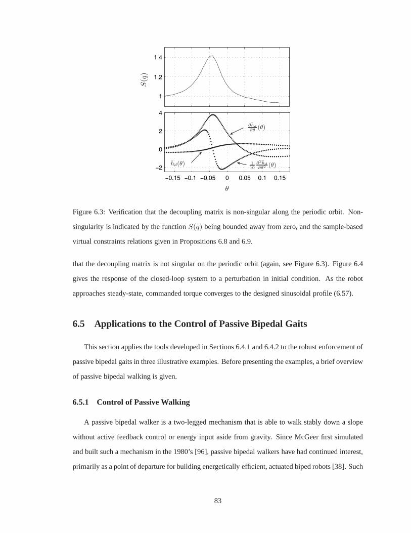
−0.15 −0.1 −0.05 0 0.05 0.1 0.15

−2

0

2

4

1

1.2

1.4

S(q

)

hd(θ)

∂hd

∂θ(θ)

110

∂2hd

∂θ2 (θ)

θ

Figure 6.3: Verification that the decoupling matrix is non-singular along the periodic orbit. Non-

singularity is indicated by the functionS(q) being bounded away from zero, and the sample-based

virtual constraints relations given in Propositions 6.8 and 6.9.

that the decoupling matrix is not singular on the periodic orbit (again, see Figure 6.3). Figure 6.4

gives the response of the closed-loop system to a perturbation in initial condition. As the robot

approaches steady-state, commanded torque converges to the designed sinusoidal profile (6.57).

6.5 Applications to the Control of Passive Bipedal Gaits

This section applies the tools developed in Sections 6.4.1 and 6.4.2 to the robust enforcement of

passive bipedal gaits in three illustrative examples. Before presenting the examples, a brief overview

of passive bipedal walking is given.

6.5.1 Control of Passive Walking

A passive bipedal walker is a two-legged mechanism that is able to walk stably down a slope

without active feedback control or energy input aside from gravity. Since McGeer first simulated

and built such a mechanism in the 1980’s [96], passive bipedal walkers have had continued interest,

primarily as a point of departure for building energetically efficient, actuated biped robots [38]. Such

83

0 0.2 0.4−3

−2

−1

0

1

(Nm

)

t (sec)0 5 10

−3

−2

−1

0

1

t (sec)

Figure 6.4: Torque evolution for a torque specified gait initialized off the orbit. Simulation is of

twenty (20) steps on level ground for the torque specified gait of Example 2. The initial error is

δx0 = (0.025, 0.0125, 3, 0). Note that the torque requirements converge rapidly to the steady-

state sinusoidal profile.

walkers, however, have two fundamentally limiting features. The first is that the basins of attraction

associated with their orbits are small—meaning passive bipedal walkers are easily toppled. The

second is a lack of variety of available walking motions; a gait’s features can only be changed by

robot redesign or by ground slope change.

Actuation can remedy both of these shortcomings. Ideal actuation10 under active feedback con-

trol can be used to increase robustness and to change a gait’scharacteristics, such as the minimum

slope on which the biped is able to walk.11 Since the energetic cost of passive dynamic walking

is, in fact, nonzero—work must be done to lift the mechanism to the top of the slope—the loss

of stable passive gaits does not preclude the use of energetic efficiency as a metric in achieving a

given objective, such as walking at a certain rate, walking on flat ground, or walking with increased

robustness.

Although the basin of attraction of the biped with the sample-based HZD controller may be

larger, the closed-loop system will, in general, not be capable of achieving a variety of different

gaits. To address this shortcoming, a constraint augmentation function can be used.

10The addition of non-ideal actuation often results in the loss of all stable, passive gaits. This is because the usualmeans of actuating a biped is with actuators that are collocated with the biped’s joints. In such a configuration, theactuator’s dynamics are coupled with the biped’s. An example where this does not occur is Collins’s powered 3D biped[38], which is powered by impulsive foot action.

11Although there do theoretically exist stable gaits for passive bipeds at arbitrarily small slopes, the basins of attractionscan be impractically small [49].

84

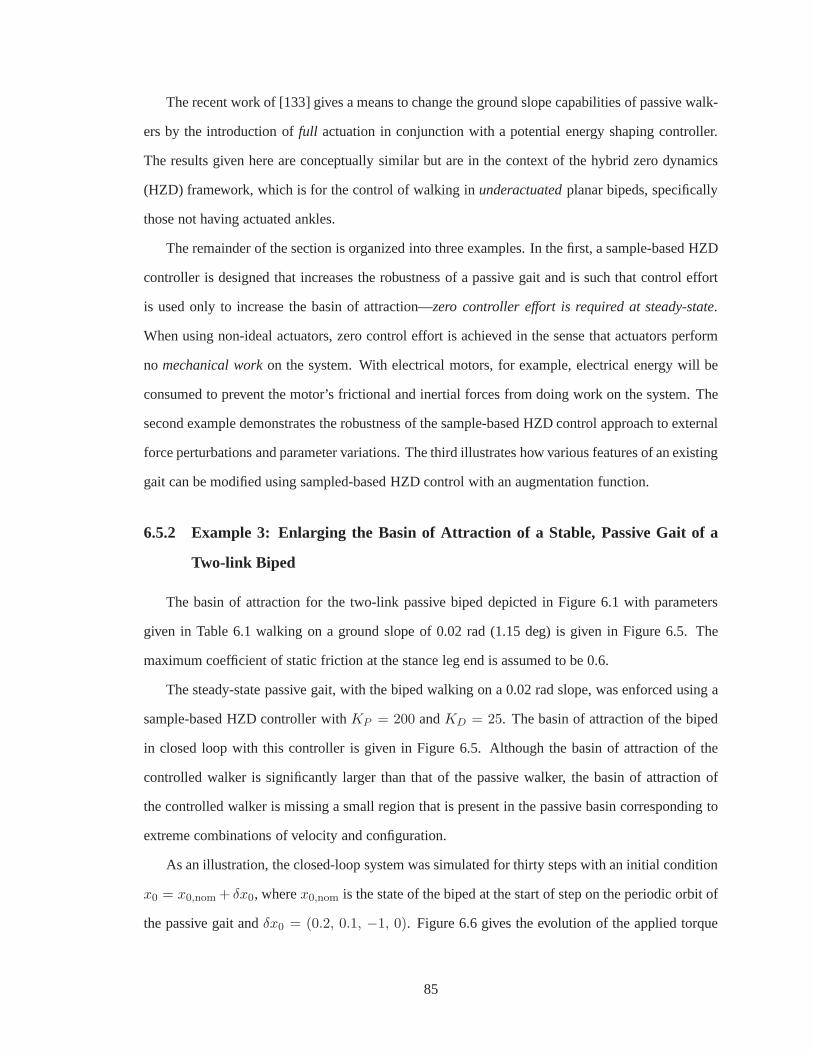
The recent work of [133] gives a means to change the ground slope capabilities of passive walk-

ers by the introduction offull actuation in conjunction with a potential energy shaping controller.

The results given here are conceptually similar but are in the context of the hybrid zero dynamics

(HZD) framework, which is for the control of walking inunderactuatedplanar bipeds, specifically

those not having actuated ankles.

The remainder of the section is organized into three examples. In the first, a sample-based HZD

controller is designed that increases the robustness of a passive gait and is such that control effort

is used only to increase the basin of attraction—zero controller effort is required at steady-state.

When using non-ideal actuators, zero control effort is achieved in the sense that actuators perform

no mechanical workon the system. With electrical motors, for example, electrical energy will be

consumed to prevent the motor’s frictional and inertial forces from doing work on the system. The

second example demonstrates the robustness of the sample-based HZD control approach to external

force perturbations and parameter variations. The third illustrates how various features of an existing

gait can be modified using sampled-based HZD control with an augmentation function.

6.5.2 Example 3: Enlarging the Basin of Attraction of a Stable, Passive Gait of a

Two-link Biped

The basin of attraction for the two-link passive biped depicted in Figure 6.1 with parameters

given in Table 6.1 walking on a ground slope of 0.02 rad (1.15 deg) is given in Figure 6.5. The

maximum coefficient of static friction at the stance leg end is assumed to be 0.6.

The steady-state passive gait, with the biped walking on a 0.02 rad slope, was enforced using a

sample-based HZD controller withKP = 200 andKD = 25. The basin of attraction of the biped

in closed loop with this controller is given in Figure 6.5. Although the basin of attraction of the

controlled walker is significantly larger than that of the passive walker, the basin of attraction of

the controlled walker is missing a small region that is present in the passive basin corresponding to

extreme combinations of velocity and configuration.

As an illustration, the closed-loop system was simulated for thirty steps with an initial condition

x0 = x0,nom + δx0, wherex0,nom is the state of the biped at the start of step on the periodic orbit of

the passive gait andδx0 = (0.2, 0.1, −1, 0). Figure 6.6 gives the evolution of the applied torque

85

δq1 (rad)

δq1

(rad

/sec

)

Figure 6.5: Basins of attraction: passive walker vs. HZD stabilized walker. Two-dimensional slices

of the initial condition basin of attraction for walking on a0.02 rad slope. The basin for the passive

walker is dark gray, the basin for the controlled walker withKP = 200 andKD = 25 is light gray,

and the basin for the controlled walker with a magnitude torque limit of 3 Nm and a coefficient of

static friction at the stance leg end of 0.6 is medium gray. Other slices of the basins of attraction are

similarly proportioned. Hereδq2 = 0. The initial conditions for Examples 3 and 5 are indicated.

u. Note that the peak control effort is relatively small and that the control effort goes to zero as the

state approaches the passive orbit.

An interesting observation is that, for this example, increased controller gains (the proportional

and derivative control gainsKP andKD) result in a smaller basin of attraction. This effect is more

pronounced for increases inKD, as can be seen in Figure 6.7. An increase in the control gains

results in larger transient control signals, and, potentially, larger ground reaction force magnitudes.

The former may result in actuator saturation, and the lattermay result in the coefficient of static

friction being exceeded.

6.5.3 Example 4: Demonstration of Robustness to External Force Perturbations and

Mass and Inertia Variations

As a test of robustness, the controlled two-link biped of Example 3 was simulated with hori-

zontal, aperiodic forces acting on its hip and swing leg end and mismatch between the model and

86

0 0.2 0.4

−0.5

0

0.5

1

1.5

(Nm

)

t (sec)0 10 20

−0.5

0

0.5

1

1.5

t (sec)

Figure 6.6: Torque evolution of walking on a slope for thirtysteps. Simulation is done assuming

a ground slope ofα = 0.02 rad using a sample-based HZD controller. Torque evolution over first

step is left and the torque evolution over all steps is right.Note that the applied torque approaches

zero as the state converges to the limit cycle. The peak torque is 1.6 Nm.

controller in leg mass,m, and leg inertia,J . Between4.6 and 4.75 seconds, a horizonal force

of 15 Nm acted at the hips opposite to the direction of forward progression, and between6.1 and

6.3 seconds a horizontal force of9.25 Nm acted at the swing leg end in the same direction as the

first. The controller’s values for the leg mass and leg inertia were set to 80% and 120%, respectively,

of the parameters given in Table 6.1. Figure 6.8 gives plots of the joint angles, joint velocities, and

joint torque. Note that because of the parameter mismatch, the steady-state control effort is no

longer zero. Also note the rather modest control effort required to reject these force perturbations.

6.5.4 Example 5: Changing the Minimum Slope Capability of a Motion

For the two-link biped of Example 3, the minimum ground sloperequired for stable walking was

found numerically (using (6.35)) to be0.0171 rad (0.980 deg). With numerical optimization, the

augmentation function depicted in Figure 6.9 was found suchthat the resulting closed-loop system

was capable of walking uphill on a slope of−0.01 rad (−0.523 deg). As an illustration, the closed-

loop system was simulated on zero slope, i.e.,α = 0, for an initial conditionx0 = x0,nom + δx0,

wherex0,nom is the state of the biped at the start of step on the periodic orbit of the passive gait on

the nominal slope,α = 0.02 rad, andδx0 = (0.025, 0.0125, 3, 0). Figure 6.10 gives the evolution

of the applied torqueu. Note that peak control effort is relatively small.

87

δq1 (rad)

δq1

(rad

/sec

)

Figure 6.7: Basins of attraction for walking on a slope with different controller gains. Two-

dimensional slices of the initial condition basin of attraction slices for walking on a 0.02 rad slope

for three different sets of controller gains. The basin for the passive walker is dark gray. The basin

with KP = 200 andKD = 25 is outlined in with a dashed line, the basin withKP = 700 and

KD = 25 is light gray, and the basin withKP = 500 andKD = 75 is medium gray. A maximum

torque limit of 3 Nm and a coefficient of static friction at thestance leg end of 0.6 were assumed.

Hereδq2 = 0.

6.6 Conclusions

This chapter presented new analysis and control tools for the control of planar bipedal walking

using hybrid zero dynamics (HZD) based control. HZD controlacts by imposing virtual constraints

on the biped’s configuration as a function of forward progression. The benefits of the HZD ap-

proach include explicit (analytical) calculation of the induced gait’s stability properties and robust

performance.

The new analysis results include analysis of the effects of walking on a slope and analysis of

dynamic (decoupling matrix) singularities. The former wasused in the design of controllers that

render passive gaits zero slope capable. The latter provides insights into the nature of constraints

that require infinite control effort to enforce, yet impose motions that are otherwise kinematically

feasible (i.e., the mechanism does not encounter a kinematic singularity).

88

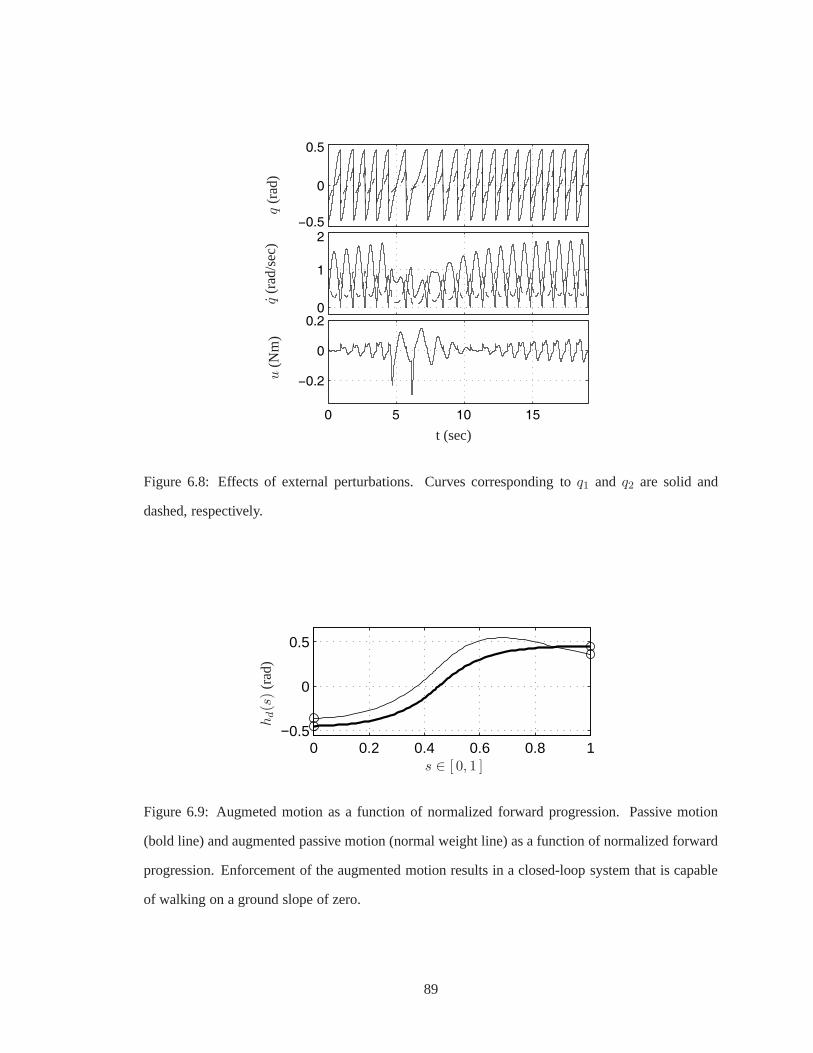
−0.5

0

0.5

0

1

2

0 5 10 15

−0.2

0

0.2

q(r

ad)

q(r

ad/s

ec)

u(N

m)

t (sec)

Figure 6.8: Effects of external perturbations. Curves corresponding toq1 and q2 are solid and

dashed, respectively.

0 0.2 0.4 0.6 0.8 1−0.5

0

0.5

s ∈ [ 0, 1 ]

hd(s

)(r

ad)

Figure 6.9: Augmeted motion as a function of normalized forward progression. Passive motion

(bold line) and augmented passive motion (normal weight line) as a function of normalized forward

progression. Enforcement of the augmented motion results in a closed-loop system that is capable

of walking on a ground slope of zero.

89

0 0.5

−2

−1.5

−1

−0.5

0

0.5

(Nm

)

t (sec)0 10 20

−2

−1.5

−1

−0.5

0

0.5

t (sec)

Figure 6.10: A zero slope capable motion. Torque evolution for a simulation of thirty (30) steps

on zero slope using a sample-based HZD controller. Torque evolution over first step is left and the

torque evolution over all steps is right. The peak torque is 2.0 Nm.

The new control tools provide an alternative method for choosing virtual constraints via sam-

pling and interpolation. The technique was used to enlarge the basin of attraction of the gait of

a passive dynamic walker. Unlike other approaches to the robust enforcement of passive bipedal

gaits, the control acts without the need for full actuation—no actuation is assumed between the

robot and the ground. The new control tools were also used to design controllers for torque spec-

ified gaits. Constraint augmentation functions were introduced, defined as finitely parameterized

functions added to the nominal, sample-based constraints that enable the kinematic and dynamic

properties of the gait to be modified.

90

Notation Introduced in Chapter 6

Symbol Meaning Defined

l, lc, m, J ,

g0

parameters of the two-link model Table 6.1

α ground slope Figure 6.1

S switching surface; Poincare section Section 6.1.1

Σ full dynamics walking model Section 6.1.1

u control input Section 6.1.1

x = (q, q) state vector of the full dynamics Section 6.1.1

[α]functional dependence onα; emphasized with square

bracketsSection 6.1.1

qa vector of actuated coordinates Section 6.1.1

qu unactuated coordinate (scalar) Section 6.1.1

D(q) inertial matrix of the full dynamics Section 6.1.2

F [α](q, q)Coriolis, centrifugal, gravitational terms of the full

dynamicsSection 6.1.2

hd(s),

hd(θ)desired joint angles of the actuated joints Section 6.2.1

θ(q)scalar function that is a surrogate for time; monotonic overa

stepSection 6.2.1

θ+, θ− values ofθ at the beginning and ending of a gait Section 6.2.1

y = h(q) output defining virtual constraints Section 6.2.1

s(θ) normalization function forθ Section 6.2.1

Z zero dynamics manifold; constraint surface Section 6.2.1

Kp, Kd PD controller gains Section 6.2.2

LgLfh(q) decoupling matrix from inputu to outputy Section 6.2.2

91

Symbol Meaning Defined

Σzero HZD model of walking Section 6.2.3

σ angular momentum about pivot foot Section 6.2.3

z = (θ, σ) state vector of the restricted (zero) dynamics Section 6.2.3

LgLfh(q) decoupling matrix from inputv to outputy Section 6.3.2

S(q) function used to determine invertibility of decoupling matrix Section 6.3.2

I(θ, y) closed-loop virtual inertia Section 6.3.3

Iy(θ, y) virtual inertia of transverse dynamics Section 6.3.3

IRB(θ, y) rigid body inertia Section 6.3.3

IAB(θ, y)inertia associated with the articulated body angular

momentumSection 6.3.3

θs value ofθ corresponding to a singularity Section 6.3.4

Ts time from step start to singularity Section 6.3.4

a augmentation function parameter vector Section 6.4.2

92

CHAPTER 7

A Restricted Poincare Map for Determining Exponentially Stable

Periodic Orbits in the Presence of Smooth Transverse Dynamics

When the method of Poincare sections is applied in practical problems, it is very common

to see the Jacobian linearization of the Poincare map estimated numerically and the exponential

stability of a fixed point (i.e., a periodic orbit) deduced onthe basis of the eigenvalues. Although

straightforward in principle, this process can become computationally unwieldy when the dimension

of the system under study is large or when stability needs to be evaluated repeatedly as part of an

iterative procedure to design a feedback controller. In order to simplify its application to nonlinear

systems with impulse effects, this chapter develops reduced dimensionality stability tests based on

the method of Poincare sections, emphasizing the role played by(hybrid) invariance, attractivity,

andtimescale separation. Simple properties are identified that govern the stabilityof periodic orbits

that lie within hybrid zero dynamics manifolds—when the transverse dynamics of a given system is

rendered exponentially stable with a sufficiently fast convergence rate, the stability of the periodic

orbit can be evaluated on the basis of the zero dynamics alone.

The work presented in this chapter is primarily an extensionof the work on restricted Poincare

maps by Grizzle, Abba, and Plestan in [60] in which a set of hypotheses required that an invariant

manifold be rendered finite time1 attractive through a feedback that was continuous but not Lipschitz

continuous. Hybrid invariance was introduced by Westervelt, Grizzle, and Koditschek in [153], but

the requirement of a finite time converging transverse dynamics remained. The results presented

here relax this requirement to exponential convergence at a“sufficiently rapid” rate, enabling the

1See [17] for an introduction to finite time controllers.

93

use of smooth feedback controllers and the stability analysis of periodic orbits inC1 systems with

impulse effects.

If the task of weakening controller hypotheses seems mundane, consider this: as observed in

the running experiments on RABBIT in Chapter 5, the presenceof strong hypotheses on controller

properties can complicate the procedure of controller design. The property of “configuration de-

terminism” at landing, required by the HZD running controllers of [31] could not be met in the

time alloted for experiments. A failure to meet this condition necessitated the use of transition

controllers—a much simpler way of arriving at a similar stability test. The stability theorems of this

chapter are designed to have weaker hypotheses so that they are compatible with a broader range

of potentially stabilizing controllers. The strongest hypothesis of this chapter, a reliance on impact

invariance, can be achieved by the methods of Chapter 8.

The remainder of this chapter is organized as follows: Section 7.1 presents a reduced dimension-

ality stability test for periodic orbits in systems with impulse effects. Use of the theorem requires

the existence of special coordinates, a hybrid invariant manifold, and a restricted Poincare map. A

similar result is derived in Section 7.2 where these hypotheses are weakened to eliminate the re-

quirement of the existence of a particular set of coordinates. The benefits of these stability tests

are demonstrated in a case study in Section 7.4. Both sets of hypotheses are verified, and both re-

duced dimensional tests are used to evaluate the stability aperiodic orbit corresponding to RABBIT

walking on flat ground.

7.1 Coordinate Dependent Hypotheses and Stability Test

The first set of hypotheses is coordinate dependent and pertains to a family of systems with

impulse effects that depends on a real parameterǫ > 0, where for each fixed value ofǫ

Σǫ :

x = f ǫ(x) x− 6∈ S

x+ = ∆(x−) x− ∈ S

(7.1)

is aC1 system with impulse effects. Following the convention established in Chapter 3, the solution

of the autonomous systemx = f ǫ(x) is written asφǫ(t, x0), the time-to-impact function isT ǫI , and

the Poincare map isP ǫ : S → S. In addition, assume that this family of systems has a periodic

orbit, coordinate transform, and invariant manifold meeting the following hypotheses:

94

Hypotheses 7.1:

i) There exist global coordinatesx = (z, η) for X ⊂ IRn, such thatz ∈ IRk, andη ∈ IRn−k,

1 < k < n, in which f ǫ has the form

f ǫ(x) = f ǫ(z, η) =

f1:k(z, η)

f ǫk+1:n(η)

;

ii) the setZ = {(z, η) ∈ X | η = 0} is such thatS∩Z is a(k−1)-dimensional,C1-embedded

submanifold satisfying the property that

∆(S ∩ Z) ⊂ Z; (7.2)

iii) the autonomous systemΣǫ has a periodic orbitO that is contained inZ, and hence the

orbit is independent ofǫ;

iv) x∗ = O ∩ S ∩ Z is a singleton;

v) LfǫH(x∗) 6= 0; and

vi) f ǫk+1:n(η) = A(ǫ)η with limǫց0 eA(ǫ) = 0.

The above conditions can be interpreted as follows: Hypotheses H7.1-i and H7.1-vi imply that

the setZ is invariant under the continuous part of the model,x = f ǫ(x), so that ifx0 ∈ Z then for

all t in its maximal domain of existence,φǫ(t, x0) ∈ Z. Hypothesis H7.1-ii implies thatZ remains

invariant across the impact event. Together, H7.1-i and H7.1-ii show that the restriction ofΣǫ to

the manifoldZ is a well-defined system with impulse effects, which will be called therestriction

dynamics,

Σǫ|Z :

z = f ǫ|Z(z) z− 6∈ S ∩ Z

z+ = ∆|Z(z−) z− ∈ S ∩ Z.

(7.3)

Hybrid invariance ofZ further implies that

P ǫ(S ∩ Z) ⊂ S ∩ Z. (7.4)

From H7.1-iii,O is a periodic orbit of the restriction dynamics that is period-one by H7.1-iv. The

restriction off ǫ toZ removes any dependence onǫ. This fact can be used to show thatφZ = φǫ|Z ,

TI,Z = T ǫI |Z , andP ǫ|Z are also independent ofǫ, and hence,

t∗ = T ǫI (∆(x∗)) (7.5)

= TI,Z(∆Z(x∗)), (7.6)

95

is independent ofǫ. On the basis of (7.4), therestricted Poincare map, ρ : S ∩ Z → S ∩ Z, can be

defined asρ = P ǫ|Z , or equivalently,

ρ(z) = φZ(TI,Z ◦ ∆Z(z),∆Z (z)), (7.7)

and is independent ofǫ. From H7.1-iv, it follows thatx∗ is a fixed point ofP ǫ andρ, and from

H7.1-v, the orbit is transversal toS, and hence also toS ∩ Z. Hypothesis H7.1-vi says that the

dynamics transversal toZ is “strongly” exponentially contracting with the rate of convergence

becoming arbitrarily fast asǫ decreases to zero. When the solution of (7.1) is not on the periodic

orbit, η(t) 6= 0. In many situations, such as bipedal walking, the impact mapincreases the norm ofη

at each impact; see Figure 7.5. Hypothesis H7.1-vi providescontrol over the speed with whichη(t)

converges to zero during the continuous phase, so that, overa cycle consisting of an impact event

followed by continuous flow, the solution may converge to theorbit. Based on these hypotheses, a

reduced dimensional stability test is given by the following theorem:

Theorem 7.2(Coordinate Dependent Reduced Dimensional Stability Test). Under Hypotheses

H7.1, there existsǫ > 0 such that for0 < ǫ < ǫ, the following are equivalent:

i. x∗ is an exponentially stable fixed point ofρ;

ii. x∗ is an exponentially stable fixed point ofP ǫ.

In other words, forǫ > 0 sufficiently small, an exponentially stable periodic orbitof the re-

striction dynamics is also an exponentially stable periodic orbit of the full order model. The proof

is based on evaluatingDP ǫ(x∗), the linearization of the Poincare map about the fixed point, in a

set of local coordinates. This is a commonly employed technique even for systems with impulse

effects [55, 141, 90, 39]. The usual approach to finding the eigenvalues ofDP ǫ(x∗) is to smoothly

extend the domain ofP ǫ from S to X and then to evaluate the linearization of the resultingn × n

Jacobian linearization. It must subsequently be shown thatone of the eigenvalues of this matrix is

always equal to unity and the remainingn − 1 eigenvalues are those ofDP ǫ(x∗) : Tx∗S → Tx∗S;

see [106, 70]. Here, local coordinates onS will be used so thatDP ǫ(x∗) is computed directly as

an(n − 1) × (n − 1) matrix. This method will give an expression forDP ǫ(x∗) that brings out its

structure due to Hypotheses H7.1.

96

7.2 Coordinate-Free Hypotheses and Stability Test

A stability test similar to the one above can be achieved under a much weaker set of hypotheses.

In this case assume there exists a system

Σ :

x = f(x) x− 6∈ S

x+ = ∆(x−) x− ∈ S,

(7.8)

for which there are setsO ⊂ X andZ ⊂ X such that

Hypotheses 7.3:

i) Z is hybrid invariant;

ii) S ∩ Z is aC1 embedded submanifold and has dimension one less thanZ; and

iii) O is a periodic orbit that is transversal toS and is contained inZ.

The list in H7.3 is a weaker set of hypotheses than H7.1. Condition H7.3-i is implied by H7.1-i,

H7.1-ii, and H7.1-vi. Condition H7.3-ii is implied by H7.1-ii, and H7.3-iii is implied by H7.1-iii.

The benefit of these weaker hypotheses is that they are easierto meet in practice. The drawback is

that the following theorem and its proof are somewhat more abstract.

Theorem 7.4 (Structure of the Linearized Return Map). Consider aC1 autonomous system

with impulse effectsΣ = (X ,S,∆, f) and assume there exists aC1 embeddedk-dimensional

submanifoldZ such that H7.3 are satisfied. Then, there exist local changesof coordinates

Γ : U → IRk−1 × IRn−k and Ψ : V → IRk × IRn−k, aboutx∗ = O ∩ S and ∆(x∗), respectively,

such that when the Poincare map of the systemΣ is represented in the new coordinates, its Jacobian2

about the fixed pointx∗ is

DP (z∗, η∗) =

Dρ(z∗) ⋆

0 SφTI(z∗, η∗)S∆(z∗, η∗)

, (7.9)

where3 P = Γ◦P ◦Γ−1, ρ is the restricted map of(7.7), SφTI(z∗, η∗) = D2(Γ2◦φTI

◦Ψ−1)(z∗, η∗),

and S∆(z∗, η∗) = D2(Ψ2 ◦ ∆ ◦ Γ−1)(z∗, η∗), for (z∗, η∗) = (Γ1(x∗),Γ2(x

∗)) = Γ(x∗) and

(z∗, η∗) = Ψ ◦ ∆(x∗) = (Ψ1 ◦ ∆(x∗),Ψ2 ◦ ∆(x∗)).

2For a differentiable functiong(x1, x2, ..., xp), the notationDig(y1, y2, ..., yp) refers to ∂g/∂xi evaluated at(x1, x2, ..., xp) = (y1, y2, ..., yp). The argumentxi may be a vector.Dg(y1, ..., yp) is (∂g/∂x1, . . . , ∂g/∂xp) evaluatedat (x1, ..., xp) = (y1, ..., yp).

3Γ1(x) andΓ2(x) refer to the firstk − 1 and lastn − k coordinates ofΓ(x), andΨ1(x) andΨ2(x) refer to the firstk and lastn − k coordinates ofΨ(x), respectively.

97

The above theorem identifies two features present in the linearized Poincare map when it is

evaluated at a fixed point lying in a hybrid invariant manifold. The first is the upper triangular struc-

ture, which is immediate from the hybrid invariance ofZ; see (7.4). The second, more interesting

result is that the bottom right block is the product ofSφTIandS∆, which are the sensitivities of the

transverse dynamics with respect to the continuous flow and impact map, respectively. If either of

the sensitivitiesSφTIor S∆ can be made sufficiently small, then the spectral radius ofDP will be

determined solely by the restricted Poincare map. Corollary 7.6 below is based on the observation

that continuous flow sensitivity,SφTI, can be made arbitrarily small through sufficiently rapid con-

vergence of the transverse dynamics. Chapter 8 will addressS∆ by showing that this term can be

made arbitrarily small by controlling the behavior of the impact map.

To develop a second reduced dimensional stability test, assume there exists a family of systems,

Σǫ :

x = f ǫ(x) x− 6∈ S

x+ = ∆(x−) x− ∈ S,

(7.10)

for which there exist setsO ⊂ X andZ ⊂ X satisfying H7.3 and also satisfying the following

Hypotheses 7.5:

i) the submanifoldZ and fixed pointx∗ are independent ofǫ;

ii) f ǫ restricted toZ is independent ofǫ; and

iii) there exists a functionK : (0,∞) → [0,∞) such thatlimǫց0 K(ǫ) = 0, and∀ ǫ > 0, ∃

δ > 0 such that4

∀ x0 ∈ Bδ(∆(x∗)), dist(φTI

ǫ(x0),Z) ≤ K(ǫ) dist(x0,Z).

The fact that H7.5-i and H7.5-ii are implied by H7.1-i, H7.1-ii, and H7.1-iii is obvious. Less

obvious is the connection between H7.5-iii and H7.1-vi. Hypothesis H7.5-iii can be interpreted as

a Lipschitz bound describing the relationship between the distance to the manifoldZ just after an

impact and the distance to the manifoldZ just before the next impact. This hypothesis is claiming

that the flow of the system is attracted to the manifoldZ in a way that is uniform with respect to

the initial distance, but not necessarily uniformly with respect to time. Also notice that H7.5-iii is a

statement about pre- and post-impact boundary conditions,whereas H7.1-vi is a statement about an

4Throughout this chapter, the notationBr(x) refers to an open ball of radiusr about the pointx.

98

entire transverse dynamics. The following corollary showshow these weaker hypotheses are used

to achieve virtually the same stability test as developed inTheorem 7.2.

Corollary 7.6 (Coordinate Independent Reduced Dimensional Stability Test). Consider a fam-

ily of C1 autonomous systems with impulse effects,Σǫ =(X ,S,∆, f ǫ

), with the vector field of

each member depending on a real parameterǫ > 0. Assume that for each value ofǫ ∈ (0,∞), Hy-

potheses H7.3 and H7.5 are met. Then the restriction dynamics Σǫ|Z =(Z,S ∩ Z,∆|S∩Z , f ǫ|Z

)

is independent ofǫ. In addition, there existsǫ > 0 such that for0 < ǫ < ǫ, the following are

equivalent:

i) x∗ is an exponentially stable fixed point ofρ, and

ii) x∗ is an exponentially stable fixed point ofP ǫ.

The proof of the corollary is given in the appendix and shows that H7.5-iii is sufficient for

achievinglimǫց0 SǫφTI

= 0. In other words, forǫ > 0 sufficiently small, an exponentially stable

periodic orbit of the restriction dynamicsΣǫ|Z =(Z,S ∩ Z,∆|S∩Z , f ǫ|Z

)is an exponentially

stable periodic orbit of the full modelΣǫ =(X ,S,∆, f ǫ

).

7.3 Feedback Design to Meet Stability Hypotheses

The next result shows how to construct a closed-loop system meeting the hypotheses of Corol-

lary 7.6. Given a control system with impulse effects,

Σ :

x = f(x) + g(x)u x− 6∈ S

x+ = ∆(x−) x− ∈ S,

(7.11)

assume there exists an output functionh such that the following are satisfied:

Hypotheses 7.7:

i) h(x) has uniform vector relative degreek;

ii) there exists a pointx such thath(x) = 0, Lfh(x) = 0, . . . , Lk−1f h(x) = 0; and

iii) the distributionspan{g1(x), · · · , gm(x)} is involutive.

99

Corollary 7.8 (Feedback Design for Reduced Dimension Stability Testing).Given a control

system with impulse effectsΣ = (X ,S, ∅,U ,∆, f, g) and a smooth outputh : X → IRm satisfying

Hypotheses H7.7 the following hold:

i) the setZ = {x ∈ X | h(x) = 0, Lfh(x) = 0, · · · , Lk−1f h(x) = 0} is a smooth embedded

submanifold ofX ,

ii) for any ǫ > 0 and scalar constantsK0, . . . ,Kk−1 chosen so thatsk + Kk−1sk−1 + · · ·+ K0

is Hurwitz, the feedback

uǫ(x) = −(

LgLk−1f h(x)

)−1(

Lkfh(x) +

∑k−1i=0

1ǫk−i KiL

ifh(x)

)

, (7.12)

applied toΣ rendersZ forward invariant in the family of closed-loop systems

Σǫ =(X ,S,∆, f ǫ

)

for f ǫ(x) = f(x) + g(x)uǫ(x); and

iii) the family of systemsΣǫ and the manifoldZ satisfy conditions H7.5.

The most significant contribution of the corollary is the interpretation that for a broad class of

feedbacks (7.12), Hypotheses H7.7 imply the satisfaction of Hypotheses H7.5. Corollaries 7.6 and

7.8 provide precise guidelines for designing a closed-loopsystem where the stability of a periodic

orbit can be determined on the basis of a restriction dynamics. This result is similar to that of

Theorem 7.2, but is stated without reference to a specific setof coordinates.

7.4 Case Study: RABBIT Walking on Flat Ground

The following example shows in detail how the theorems of this section can be used to design

controllers to induce stable walking on flat ground in a 5 DOF bipedal model resembling the biped

RABBIT. Both the coordinate dependent hypotheses of Theorem 7.2 and the coordinate independent

hypotheses of Theorem 7.4 and its corollaries will be verified. This comparison will help to highlight

the differences between the two proposed methods of reduceddimensionality stability testing.

100

7.4.1 Open-Loop Model

A model of RABBIT with coordinatesq = (q1, . . . , q5) ∈ Q as shown in Figure 7.1 is briefly

summarized. Following [29], the method of Lagrange leads tothe standard mechanical model

D(q)q + C(q, q)q + G(q) = Bu, with B =

I

0

. (7.13)

The impact (i.e., switching) surface isS = {(q, q) ∈ X | y2(q) = 0, x2(q) > 0}, the set of points

where the swing leg height is zero and in front of the stance leg. When the swing leg contacts

the ground an inelastic collision gives rise to a jump in the velocity coordinates5. An impact map

∆ : S → X can be computed as in [74, 60, 29]. Definingx = (q, q), the mechanical model is

expressed in state variable form as a controlled system withimpulse effects:

Σ :

x = f(x) + g(x)u x− /∈ S

x+ = ∆(x−) x− ∈ S,(7.14)

where the vector of control torques isu ∈ IR4.

In [153, Section V-VII], it is shown how to design output functions y = h(x) using Bezier

polynomials and (nonconstructive) numerical optimization to meet many of the assumptions made

so far, as they relate to RABBIT: invertibility of the decoupling matrix LgLfh, impact invariance

∆(S ∩ Z) ⊂ Z, the existence of a periodic orbit lying withinZ that is transversal toS ∩ Z. These

conditions can often be met while simultaneously meeting other performance objectives involving

walking speed, actuator power, and the contact forces at theleg ends. Since RABBIT has five

degrees of freedom in the stance phase and four independent actuators, the restricted Poincare map

is scalar valued, and hence the Jacobian linearization of the restricted Poincare map is a scalar. What

remains is to design a feedback controller so that the resulting closed-loop system meets conditions

on reduced dimensionality stability testing.

7.4.2 Feedback Design

The feedback designs developed in [153] are based on virtualconstraints, which are holonomic

constraints on the robot’s configuration that are asymptotically imposed through feedback control.5So that the same mechanical model can be used independent of which leg is the stance leg, the coordinates must

also be relabeled, giving rise to a jump in the configuration variables as well; see[60, 153, 29]. The impact map satisfies∆(S) ∩ S = ∅.

101

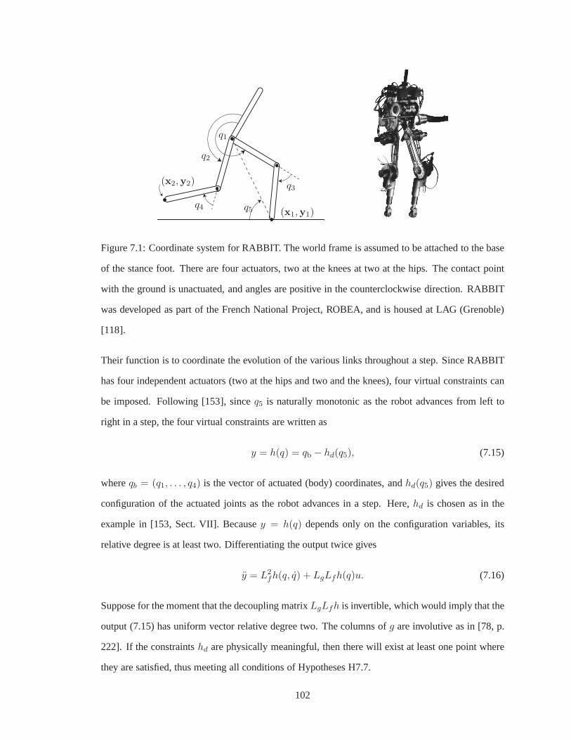
q2

q1

q4

q3

q5 (x1,y1)

(x2,y2)

Figure 7.1: Coordinate system for RABBIT. The world frame isassumed to be attached to the base

of the stance foot. There are four actuators, two at the kneesat two at the hips. The contact point

with the ground is unactuated, and angles are positive in thecounterclockwise direction. RABBIT

was developed as part of the French National Project, ROBEA,and is housed at LAG (Grenoble)

[118].

Their function is to coordinate the evolution of the variouslinks throughout a step. Since RABBIT

has four independent actuators (two at the hips and two and the knees), four virtual constraints can

be imposed. Following [153], sinceq5 is naturally monotonic as the robot advances from left to

right in a step, the four virtual constraints are written as

y = h(q) = qb − hd(q5), (7.15)

whereqb = (q1, . . . , q4) is the vector of actuated (body) coordinates, andhd(q5) gives the desired

configuration of the actuated joints as the robot advances ina step. Here,hd is chosen as in the

example in [153, Sect. VII]. Becausey = h(q) depends only on the configuration variables, its

relative degree is at least two. Differentiating the outputtwice gives

y = L2fh(q, q) + LgLfh(q)u. (7.16)

Suppose for the moment that the decoupling matrixLgLfh is invertible, which would imply that the

output (7.15) has uniform vector relative degree two. The columns ofg are involutive as in [78, p.

222]. If the constraintshd are physically meaningful, then there will exist at least one point where

they are satisfied, thus meeting all conditions of Hypotheses H7.7.

102

As described in Corollary 7.8, choose scalarsKD andKP such that

s2 + KDs + KP = 0 (7.17)

has distinct roots with negative real parts, and letǫ > 0. Then the feedback law

u(x) = −(LgLfh(x))−1

(

L2fh(x) +

1

ǫKDLfh(x) +

1

ǫ2KP h(x)

)

(7.18)

applied tox = f(x) + g(x)u results in

y = −1

ǫKDy −

1

ǫ2KP y. (7.19)

7.4.3 Closed-Loop Analysis

Having met the coordinate-free hypotheses of H7.7, Corollary 7.8 states that the set

Z = {x ∈ X | h(x) = 0, Lfh(x) = 0}

is a smooth two-dimensional submanifold ofX and is invariant under the closed-loop dynamics

f ǫ(x) = f(x) + g(x)uǫ(x).

We now turn our attention to Corollary 7.6; assume thatZ is impact invariant, thatS ∩ Z has

codimension one inZ, and that there exists a periodic orbit withinZ that is transversal toS (all

common constraints used in choosing the output function (7.15)). With H7.5 satisfied by Corollary

7.8 and H7.3 satisfied by assumption, Corollary 7.6 shows that for sufficiently smallǫ > 0, the

periodic orbit is stable in the zero dynamics if and only if itis stable in the full dynamics.

When testing stability based on Theorem 7.2, our first objective will be to putf ǫ in the proper

coordinates so that Hypotheses H7.1 can be checked. Note that becauseh(q) = qb − hd(q5),

Ψ(q) =

h(q)

q5

(7.20)

is a global diffeomorphism onQ. It follows that

z1

z2

η1:4

η5:8

=

q5

d5(q)q

h(q)

∂h∂q (q)q

(7.21)

103

is a global diffeomorphism onX = TQ, whered5 is the last row of the inertia matrixD, and

σ = d5(q)q is the angular momentum of the biped about the end of the stance leg end [29]. In these

coordinates [78, pp. 224],

f ǫ(z, η) =

f1:2(z, η)

A(ǫ)η

, (7.22)

where

A(ǫ) =

0 I4×4

−kP

ǫ2 I4×4−kD

ǫ I4×4

, (7.23)

thus meeting H7.1-i. As mentioned earlier, conditions H7.1-ii, H7.1-iii, H7.1-iv, and H7.1-v (in-

cluding impact invariance and the existence of a periodic orbit lying within Z) are ensured by

the correct selection of an output function. To verify the final hypotheses we will show that

limǫց0 eA(ǫ) = 0. Note that

A(ǫ) = Π(ǫ)1

ǫA0Π

−1(ǫ), (7.24)

where

A0 =

0 I4×4

−kP I4×4 −kDI4×4

(7.25)

and

Π(ǫ) =

ǫI4×4 0

0 I4×4

. (7.26)

Since (7.17) is a Hurwitz polynomial,

limǫց0

e1ǫA0 = 0

and hence

limǫց0

eA(ǫ) = 0,

thus fulfilling H7.1-vi. Applying Theorem 7.2, forǫ > 0 sufficiently small the feedback law (7.18)

exponentially stabilizes in the full order model a periodicorbit that is exponentially stable in the

restriction dynamics.

104

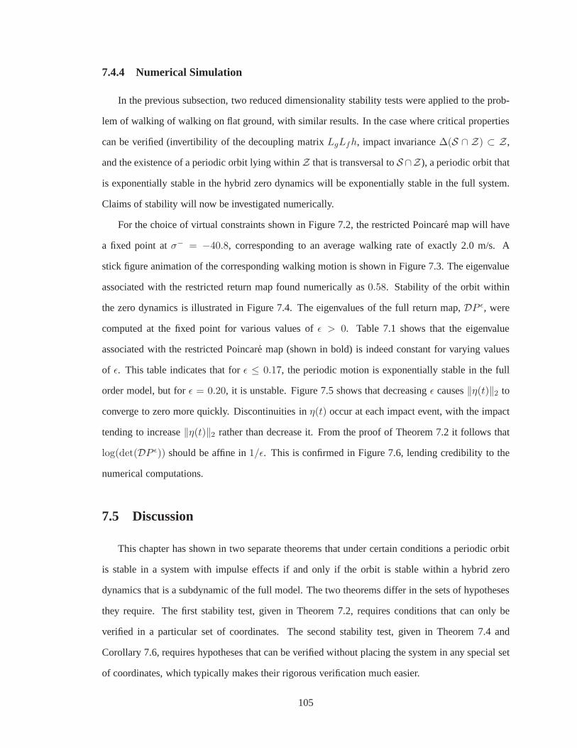
7.4.4 Numerical Simulation

In the previous subsection, two reduced dimensionality stability tests were applied to the prob-

lem of walking of walking on flat ground, with similar results. In the case where critical properties

can be verified (invertibility of the decoupling matrixLgLfh, impact invariance∆(S ∩ Z) ⊂ Z,

and the existence of a periodic orbit lying withinZ that is transversal toS ∩Z), a periodic orbit that

is exponentially stable in the hybrid zero dynamics will be exponentially stable in the full system.

Claims of stability will now be investigated numerically.

For the choice of virtual constraints shown in Figure 7.2, the restricted Poincare map will have

a fixed point atσ− = −40.8, corresponding to an average walking rate of exactly 2.0 m/s. A

stick figure animation of the corresponding walking motion is shown in Figure 7.3. The eigenvalue

associated with the restricted return map found numerically as0.58. Stability of the orbit within

the zero dynamics is illustrated in Figure 7.4. The eigenvalues of the full return map,DP ǫ, were

computed at the fixed point for various values ofǫ > 0. Table 7.1 shows that the eigenvalue

associated with the restricted Poincare map (shown in bold) is indeed constant for varying values

of ǫ. This table indicates that forǫ ≤ 0.17, the periodic motion is exponentially stable in the full

order model, but forǫ = 0.20, it is unstable. Figure 7.5 shows that decreasingǫ causes‖η(t)‖2 to

converge to zero more quickly. Discontinuities inη(t) occur at each impact event, with the impact

tending to increase‖η(t)‖2 rather than decrease it. From the proof of Theorem 7.2 it follows that

log(det(DP ǫ)) should be affine in1/ǫ. This is confirmed in Figure 7.6, lending credibility to the

numerical computations.

7.5 Discussion

This chapter has shown in two separate theorems that under certain conditions a periodic orbit

is stable in a system with impulse effects if and only if the orbit is stable within a hybrid zero

dynamics that is a subdynamic of the full model. The two theorems differ in the sets of hypotheses

they require. The first stability test, given in Theorem 7.2,requires conditions that can only be

verified in a particular set of coordinates. The second stability test, given in Theorem 7.4 and

Corollary 7.6, requires hypotheses that can be verified without placing the system in any special set

of coordinates, which typically makes their rigorous verification much easier.

105

1.3 1.4 1.5 1.6 1.7 1.8 1.93.4

3.6

3.8

4

4.2

4.4

1.3 1.4 1.5 1.6 1.7 1.8 1.90

0.5

1

1.5

θ (rad)

θ (rad)

desi

red

angl

e(r

ad)

desi

red

angl

e(r

ad) q1 stance hip

q2 swing hip

q3 stance kneeq4 swing knee

Figure 7.2: A graphical representation of the virtual constraints.

−0.6 −0.4 −0.2 0 0.2 0.4 0.6 0.8 10

0.2

0.4

0.6

0.8

1

1.2

1.4

1.6

Figure 7.3: A stick figure animation of the walking motion used in the example.

106

1.3 1.4 1.5 1.6 1.7 1.8 1.9

20

25

30

35

40

θ

|σ|

Figure 7.4: System response within the hybrid zero dynamicsmanifold. The initial condition (noted

with an asterisk) lies within the hybrid zero dynamics manifold. Convergence to the orbit is rapid,

with an estimated eigenvalue of0.58. Stability of an orbit within the zero dynamics manifold is

independent of the value ofǫ.

ǫ = 0.12 ǫ = 0.17 ǫ = 0.20

0.58 −0.62 −1.91

0.48 0.58 0.58

−0.12 + 4.4 × 10−2 i −0.19 + 0.14 i −0.12 + 0.27 i

−0.12 − 4.4 × 10−2 i −0.19 − 0.14 i −0.12 − 0.27 i

−0.11 + 5.4 × 10−2 i −0.17 + 0.16 i −0.15 + 0.25 i

−0.11 − 5.4 × 10−2 i −0.17 − 0.16 i −0.15 − 0.25 i

2.5 × 102 0.14 0.21

9.2 × 10−3 − 1.8 × 10−2 i −8.2 × 10−2 −4.2 × 10−2

9.2 × 10−3 + 1.8 × 10−2 i 8.0 × 10−3 7.6 × 10−3

Table 7.1: Eigenvalues ofDP ǫ for three values ofǫ, ranked by magnitude. The eigenvalue ofDρ is

shown in bold.

107

0 0.5 1 1.5 2

0.2

0 0.5 1 1.5 20

0.2

0.4

0.4

0 0.5 1 1.5 20

2

4

Time (s)

ǫ = 0.12

ǫ = 0.17

ǫ = 0.20

‖η‖2

‖η‖2

‖η‖2

Figure 7.5: Error profiles for three values ofǫ. The restricted system corresponds toη ≡ 0. As ǫ

decreases to zero,η(t) converges more quickly to zero. Note that the orbit is unstable for ǫ = 0.2

even though it is exponentially stable in the restricted dynamics and the “transversal part” of the

closed-loop ODE is decoupled, linear, and exponentially stable.

5 10 15 20−50

−40

−30

−20

−10

1/ǫ

log(d

et(D

Pǫ))

Figure 7.6: The graph oflog(det(DP ǫ)) versus1/ǫ. The correlation should be affine when the

controller (7.18) is used. The circles locate the numerically estimated values oflog(det(DP ǫ)) for

five different values ofǫ. The solid line is an affine fit.

108

Both of these theorems improve upon the previous work by relaxing the requirement of finite

time attractivity (previously used in theorems on restricted Poincare stability testing) with a more

general requirement for sufficiently fast exponential attractivity. This relaxation of requirements

allows a wider class of feedback control laws to be considered for the task of stabilizing locomotion

in bipedal robots. The utility of the two new theorems was highlighted in a case study. A periodic

orbit whose design was carried out on the basis of a two-dimensional restriction dynamics (i.e., the

hybrid zero dynamics of walking) could be systematically rendered exponentially stable in the full

order model by using a smooth state variable feedback, as predicted by both the coordinate-based

stability test of Theorem 7.2 and the coordinate-free stability test of Theorem 7.4 and its corollaries.

109

Notation Introduced in Chapter 7

Symbol Meaning Defined

ǫa strictly positive scalar parameter used for tuning the rate of

convergence to a hybrid invariant manifoldZSection 7.1

Σǫa family of systems with impulse effects, where for a fixed

value ofǫ, each member is aC1 system with impulse effectsSection 7.1

φǫ(t, x0) solution of the autonomous systemx = fǫ(x) Section 7.1

T ǫI (x) theǫ-dependant time-to-impact function forΣǫ Section 7.1

P ǫ(x) theǫ-dependant Poincare return map forΣǫ Section 7.1

Σǫ|Z the restriction ofΣǫ to a hybrid invariant manifoldZ Section 7.1

DP ǫ(x∗)the Jacobian linearization ofP ǫ as evaluated at the fixed

pointx∗Section 7.1

Tx∗S the tangent space ofS at the pointx∗ Section 7.1

η coordinates of the transverse dynamics Section 7.1

z coordinates of the zero dynamics Section 7.1

DP (z∗, η∗)the Jacobian linearization of a Poincare map for an au-

tonomous system with impulse effects, written in special co-

ordinates

Section 7.2

Γ, Ψ coordinate transforms proposed by Theorem 7.4 Section 7.2

SφTI

sensitivity of the transverse dynamics to the continuous flow

of an autonomous system with impulse effectsSection 7.2

S∆

sensitivity of the transverse dynamics to the impact map of

an autonomous system with impulse effectsSection 7.2

110

CHAPTER 8

Parameter Updates for Achieving Impact Invariance

In the context of systems with impulse effects, hybrid invariance occurs when a manifold is

invariant under both the continuous (ODE) portion and the discrete (impact) map of the model.

Chapter 7 has shown that the property of hybrid invariance can significantly reduce the computa-

tional burden associated with testing the stability of a periodic orbit in a system with impulse effects.

In the special case of models based on RABBIT, designing hybrid invariant manifolds is quite easy

because of special structures that arise when the virtual constraints have uniform vector relative

degree two, and previously published works in hybrid zero dynamics only address these types of

outputs. In the case of robots with series springs, relevantoutputs do not necessarily have uniform

vector relative degree two, and achieving hybrid invariance is much more difficult.

Forward invariance in ODE models is a rich, well-studied subject. In particular the methods

developed by Byrnes and Isidori in the area ofzero dynamicscan be used to design forward invariant

manifolds, not necessarily resulting from outputs having uniform vector relative degree two. A less

well-studied and hence more challenging problem is how to achieve impact invariance in more

general classes of output functions than those previously considered. To address the problem, this

chapter introduces the tool ofparameterized extensions, a type of dynamic extension for systems

with impulse effects. With the introduction of parameterized outputs, a discrete feedback element

becomes available—the parameter update law. When used properly, a discrete feedback controller

can provide impact invariance, with a separately designed continuous feedback controller providing

forward invariance.

A valid concern when using parameter update schemes is the potential for introducing unstable

111

modes into the system. Albeit discrete, unstable parameterdynamics could destabilize an otherwise

stable system control system. For this reason, the proposedhybrid extensions aredeadbeat, or put

differently, memoryless in the parameters. Deadbeat parameter extensions introduce no additional

dynamics, discrete or continuous, stable or unstable.

The remainder of this chapter gives two solutions for achieving impact invariance of manifolds

resulting from outputs having arbitrary uniform vector relative degree. Under the assumption that

an appropriate parameter update function can be found, Section 8.2 presents a deadbeat hybrid

extension for achieving impact invariance. Because derivation of this function is often difficult, the

result of Section 8.3 provides an alternative solution for achieving impact invariance, one in which

the original output function is modified so that the parameter update scheme is known in closed

form. The closed-loop properties of both parameter update schemes are explored in Chapter 9 in a

case study examining walking in a planar robot with compliance.

8.1 Definition and Properties of Parameter Extensions

Let Σ = (X ,S, ∅,U ,∆, f, g) be a control system with impulse effects1 and letA be an open

subset ofIRq, q ≥ 1. Then, the system

Σe :

(x, α) = (f(x) + g(x)u, 0) (x−, α−) 6∈ S × A

(x+, α+) = (∆(x−), v) (x−, α−) ∈ S ×A

(8.1)

is called aparameterized extensionof Σ and can be denoted in alternative notation as

Σe = (Xe,Se,A,U ,∆e, fe, ge)

(with elements of the 7-tupleΣe defined in the obvious way). When a parameter update law is

chosen to be independent of the parameter itself, that is,∆v : S → A, the resultant system

Σe =(Xe,Se, ∅,U , ∆e, fe, ge

)

with ∆e(xe) = (∆(x),∆v(x)) andxe = (x, α), is called anopen-loop deadbeat hybrid extension.

A closed-loop deadbeat hybrid extensionis an autonomous system denoted

Σe =(Xe,Se, ∆e, fe

)

1Note thatV = ∅, indicating an absence of control authority over the impactmap.

112

wherefe(xe) = fe(xe) + ge(xe)u(xe) for some state feedback lawu : Xe → U .

8.2 Nonconstructive Parameter Extensions for Hybrid Invariance

One critical aspect of applying Theorems 7.2 or 7.4 in the context of bipedal locomotion is the

selection of an outputh(x) that leads to a hybrid invariant manifold. Appropriately choosing an out-

put so that its zeroing manifold is impact invariant is a nontrivial task, in general. In previous work,

[153, Section V, Thm. 4] identified a class of holonomic2, uniform vector relative degree two outputs

for which it is straightforward to meet the impact invariance condition. The reasoning employed in

[153] relied heavily on the fact that both the impact map∆ andLfh were linear in the generalized

velocity coordinate. This linearity property breaks down already forL2fh (equivalently, for outputs

with uniform vector relative degree, which are relevant in the context of compliant actuation). With-

out linearity of both the boundary conditions of the virtualconstraints and the impact map itself,

giving verifiable conditions for impact invariance can become hard. The following remark gives a

restatement of the condition of impact invariance that is more amenable to the development of a

parameter update law leading to impact invariance.

Remark 8.1. When a system with impulse effects

Σ :

x = f(x) + g(x)u x− 6∈ S

x+ = ∆(x−) x− ∈ S,

(8.2)

has an outputh(x) with uniform vector relative degreek, with

Z = {x ∈ X | h(x) = 0, Lf h(x) = 0, · · · , Lk−1f h(x) = 0},

then the following are equivalent:

a) ∆(S ∩ Z) ⊂ Z;

b) ∀x ∈ ∆(S ∩ Z) and∀0 ≤ i ≤ k − 1, Lifh(x) = 0.

If the output functionh(x) is dependent on a vector of realsα ∈ A ⊂ IRq and the setS ∩ Z

is independent ofα, then conditionb) above can be restated as a condition on controlled impact

2The output functionh depended only on the configuration variables of the robot, hence the terminology “holonomic”.

113

invariance:

∀x ∈ ∆(S ∩ Z) ∃α ∈ A such thatLifh(x, α) = 0 ∀0 ≤ i ≤ k − 1. (8.3)

The following theorem illustrates the use of a parameter update law to achieve the controlled in-

variance described above. Under the given conditions, the extra dimensionality associated with the

parameters does not significantly complicate the Poincarereturn map. The theorem is labeled as

“nonconstructive” because no closed form parameter updatescheme is given.

Theorem 8.2(Invariance by Nonconstructive Deadbeat Hybrid Extension). Consider aC1 sys-

tem with impulse effects

Σ :

x = f(x) + g(x)u x− 6∈ S

x+ = ∆(x−) x− ∈ S

(8.4)

with ann-dimensional state manifoldX andm-dimensional inputsu. LetA be an open subset of

IRq, for someq ≥ 1, and leth : X ×A → IRm be an output function. Suppose furthermore that

Hypotheses 8.3:

i) ∀α ∈ A, the outputy = h(x, α) has uniform vector relative degreek;

ii) there exists a non-emptyC1 submanifoldZ such that∀α ∈ A,

Zα = {x ∈ X | h(x, α) = 0, · · · , Lk−1f h(x, α) = 0}

is diffeomorphic toZ;

iii) S ∩ Zα is independent ofα and equalsS ∩ Z;

iv) S ∩ Z is C1 and has dimension one less thanZ; and

v) there exits aC1 function∆v : S → A such that,∀x ∈ S ∩ Z, the valuesξ = ∆(x),

α = ∆v(x) result in

h(ξ, α) = 0

Lfh(ξ, α) = 0

. . .

Lk−1f h(ξ, α) = 0.

114

Then for anyǫ > 0 the closed-loop deadbeat hybrid extension,

Σǫe :

(x, α) = (f(x) + g(x)uǫ(x, α), 0) (x−, α−) 6∈ S × A

(x+, α+) = (∆(x−),∆v(x−)) (x−, α−) ∈ S ×A

(8.5)

with feedbackuǫ(x, α) modified from(7.12)

uǫ(x, α) = −(

LgLk−1f h(x, α)

)−1(

Lkfh(x, α) +

∑k−1i=0

1ǫk−i KiL

ifh(x, α)

)

, (8.6)

has a hybrid zero dynamicsΣǫe|Ze

. Moreover,

a) the hybrid zero dynamics manifold of(8.5) isZe = ∪α∈A(Zα, α),

b) Ze ∩ (S ×A) = (S ∩ Z) ×A, and

c) the Poincare mapP ǫe |Ze

: (S ∩ Z) ×A → (S ∩ Z) ×A for the restriction dynamics is

P ǫe |Ze

(z, α) = (ρe(z),∆v(z)), (8.7)

whereρe : S ∩ Z → S ∩ Z is independent ofǫ.

Remark 8.4. Suppose thatΣ = (X ,S, ∅,U ,∆, f, g) has a periodic orbitO. Define the parameter

vectorα∗ = ∆v(x∗) for x∗ = O∩S. Then the setOe = O × α∗ is a periodic orbit of the open-loop

deadbeat hybrid extensionΣe. The orbitOe will be called the trivial lift ofO into Σe.

Given an appropriate parameter update function∆v, the above theorem shows how to construct

a deadbeat hybrid extension to produce a hybrid invariant manifold. The restricted Poincare map

P ǫe |Ze

(z, α) has the additional property that its spectral radius is determined solely by the properties

of ρ(z, a). Using Theorem 8.2, observe that

∂ P ǫe |Ze

(z, α)

∂(z, α)=

∂ρe(z)∂z

∂ρe(z)∂α

∂∆v(z)∂z

∂∆v(z)∂α

=

∂ρe(z)∂z 0

∂∆v(z)∂z 0

(8.8)

and notice that

max

∣∣∣∣eig

(∂ P ǫ

e |Ze(z, α)

∂(z, α)

)∣∣∣∣= max

∣∣∣∣eig

(∂ρe(z)

∂z

)∣∣∣∣. (8.9)

Stability implications of (8.8) and (8.9) will be investigated in the next section.

A major drawback of Theorem 8.2 is that the control designer must first find a satisfactory

∆v before the theorem can be applied. Hypothesis H8.3-v gives aclear statement of the required

115

properties of∆v but provides no insight into its selection. The following proposition, stated without

proof, describes conditions under which a satisfactory∆v is known to exist. As the result depends

on the Implicit Function Theorem, the proposition asserts only existence of the parameter update

function and does not provide its closed-form expression.

Proposition 8.5. If there exists a periodic orbitO and a vectorα = α∗ on which the outputh(x, α)

is identically zero, and the Jacobian

∂

∂α

h(ξ, α)

Lfh(ξ, α)

. . .

Lk−1f h(ξ, α).

ξ = ∆(x∗)

α = α∗

(8.10)

has full row rank, then by the Implicit Function Theorem there exists a parameter update function

∆v : S → A such that∀x ∈ S ∩ Z, the valuesξ = ∆(x), α = ∆v(x) result in

h(ξ, α) = 0

Lfh(ξ, α) = 0

. . .

Lk−1f h(ξ, α) = 0.

A different method for achieving hybrid invariant manifolds is presented in the following sec-

tion. The result involves the use of deadbeat hybrid extensions, but outputs are chosen in such a

way that leads to a closed-form expression of the required parameter update law.

8.3 Constructive Parameter Extensions for Hybrid Invariance

Theorem 8.6(Impact Invariance by Construction). Consider a smooth control system with im-

pulse effects3 Σ = (X ,S, ∅,U ,∆, f, g), withU ⊂ IRm. Assume there exists a periodic orbitO that

is transversal toS and that in addition

Hypotheses 8.7:

3Once again note thatV = ∅, indicating an absence of control authority over the impactmap.

116

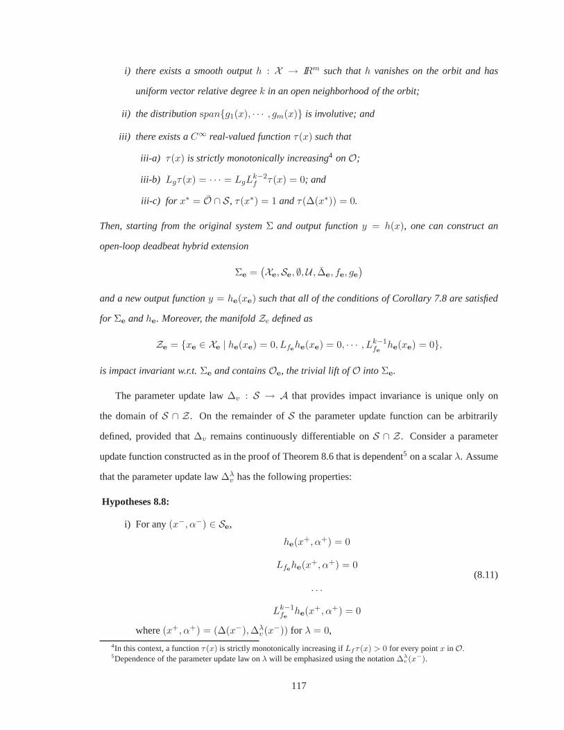
i) there exists a smooth outputh : X → IRm such thath vanishes on the orbit and has

uniform vector relative degreek in an open neighborhood of the orbit;

ii) the distributionspan{g1(x), · · · , gm(x)} is involutive; and

iii) there exists aC∞ real-valued functionτ(x) such that

iii-a) τ(x) is strictly monotonically increasing4 onO;

iii-b) Lgτ(x) = · · · = LgLk−2f τ(x) = 0; and

iii-c) for x∗ = O ∩ S, τ(x∗) = 1 andτ(∆(x∗)) = 0.

Then, starting from the original systemΣ and output functiony = h(x), one can construct an

open-loop deadbeat hybrid extension

Σe =(Xe,Se, ∅,U , ∆e, fe, ge

)

and a new output functiony = he(xe) such that all of the conditions of Corollary 7.8 are satisfied

for Σe andhe. Moreover, the manifoldZe defined as

Ze = {xe ∈ Xe | he(xe) = 0, Lfehe(xe) = 0, · · · , Lk−1fe

he(xe) = 0},

is impact invariant w.r.t.Σe and containsOe, the trivial lift of O into Σe.

The parameter update law∆v : S → A that provides impact invariance is unique only on

the domain ofS ∩ Z. On the remainder ofS the parameter update function can be arbitrarily

defined, provided that∆v remains continuously differentiable onS ∩ Z. Consider a parameter

update function constructed as in the proof of Theorem 8.6 that is dependent5 on a scalarλ. Assume

that the parameter update law∆λv has the following properties:

Hypotheses 8.8:

i) For any(x−, α−) ∈ Se,

he(x+, α+) = 0

Lfehe(x+, α+) = 0

. . .

Lk−1fe

he(x+, α+) = 0

(8.11)

where(x+, α+) = (∆(x−),∆λv (x−)) for λ = 0,

4In this context, a functionτ (x) is strictly monotonically increasing ifLfτ (x) > 0 for every pointx in O.5Dependence of the parameter update law onλ will be emphasized using the notation∆λ

v (x−).

117

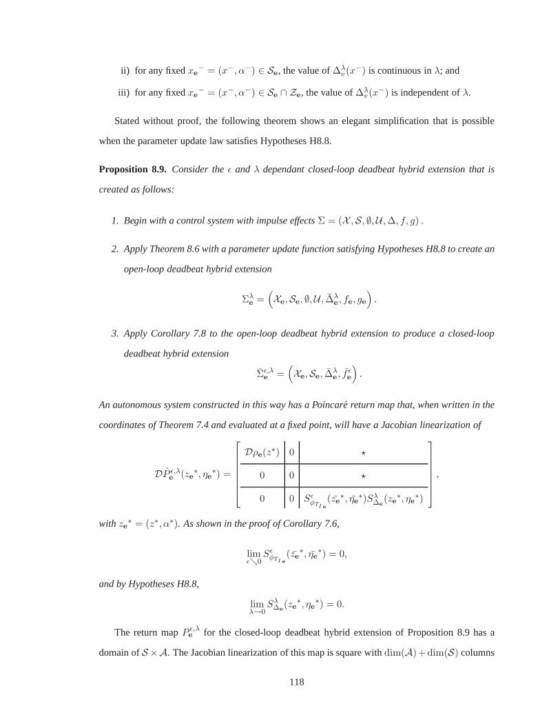
ii) for any fixedxe− = (x−, α−) ∈ Se, the value of∆λ

v (x−) is continuous inλ; and

iii) for any fixedxe− = (x−, α−) ∈ Se ∩ Ze, the value of∆λ

v (x−) is independent ofλ.

Stated without proof, the following theorem shows an elegant simplification that is possible

when the parameter update law satisfies Hypotheses H8.8.

Proposition 8.9. Consider theǫ and λ dependant closed-loop deadbeat hybrid extension that is

created as follows:

1. Begin with a control system with impulse effectsΣ = (X ,S, ∅,U ,∆, f, g) .

2. Apply Theorem 8.6 with a parameter update function satisfying Hypotheses H8.8 to create an

open-loop deadbeat hybrid extension

Σλe =

(

Xe,Se, ∅,U , ∆λe , fe, ge

)

.

3. Apply Corollary 7.8 to the open-loop deadbeat hybrid extension to produce a closed-loop

deadbeat hybrid extension

Σǫ,λe =

(

Xe,Se, ∆λe , f ǫ

e

)

.

An autonomous system constructed in this way has a Poincare return map that, when written in the

coordinates of Theorem 7.4 and evaluated at a fixed point, will have a Jacobian linearization of

DP ǫ,λe (ze

∗, ηe∗) =

Dρe(z∗) 0 ⋆

0 0 ⋆

0 0 SǫφTI e

(ze∗, ηe

∗)Sλ∆e

(ze∗, ηe

∗)

,

with ze∗ = (z∗, α∗). As shown in the proof of Corollary 7.6,

limǫց0

SǫφTI e

(ze∗, ηe

∗) = 0,

and by Hypotheses H8.8,

limλ→0

Sλ∆e

(ze∗, ηe

∗) = 0.

The return mapP ǫ,λe for the closed-loop deadbeat hybrid extension of Proposition 8.9 has a

domain ofS ×A. The Jacobian linearization of this map is square withdim(A)+dim(S) columns

118

and rows. To test the stability of this return map (without utilizing any of its special properties)

would require checking the eigenvalues of a(dim(A) + dim(S)) × (dim(A) + dim(S)) matrix.

In contrast, if a feedback controller were designed directly for the original control system with

impulse effects considered in Proposition 8.9, the resulting autonomous system would not have

an accompanying parameter spaceA, and thus the Poincare return map would have a domain of

S. To test the stability properties of this return map would require checking the eigenvalues of a

dim(S) × dim(S) matrix.

What then is the benefit of parameter augmentation? Proposition 8.9 shows that the Jacobian

linearization ofP ǫ,λe , when evaluated at the fixed point and written in special coordinates, has a

structure such that

max |DP ǫ,λe (ze

∗, ηe∗)| = max |eig(Dρe(z

∗))|,

for ǫ andλ constant and sufficiently close to zero. The stability of thereturn mapDP ǫ,λe (ze

∗, ηe∗)

is determined by the eigenvalues of the(dim(S ∩ Z)) × (dim(S ∩ Z)) Jacobian linearization

of Dρe(z∗), showing that parameter augmentation does not complicate the reduced dimensional

stability tests of Chapter 7.

8.4 Discussion

Motivated by the problem of creating exponentially stable periodic orbits in bipedal robots with

underactuation and actuator dynamics, Chapter 7 extended the hybrid zero dynamics (HZD) frame-

work of [153] to nonlinear systems with impulse effects where the outputs have vector relative

degree greater than two. Describing the required conditions of simultaneous invariance under the

continuous dynamics and the impact map was straightforward.

The more challenging aspect of the extension is addressed inthis chapter—how to meet the

impact invariance condition when the relative degree is greater than two. The result on impact

invariance in [153] could not be extended in a direct way. A novel embedding of the original system

into a system with event-based parameter updates was therefore introduced. The additional dynamic

elements in the larger system can be tailored to meet the boundary conditions associated with impact

invariance. This result was formalized in Theorem 8.2, which gave a nonconstructive solution for

the impact map yielding impact invariance. The proposed dynamic extension is deadbeat in that the

119

additional states are updated only at impacts, and their newvalues depend only on the states of the

original system, not the previous values of the parameters.

Based strongly on spline-like transition functions, the constructive outputs proposed in Theorem

8.6 allow the use of a constructive parameter update law thatleads to impact invariance. Although

both improve upon previously published results, the constructive solution of Theorem 8.6 is a far

more powerful solution than its nonconstructive counterpart, Theorem 8.2.

Overall this chapter demonstrates the important fact that impact invariance can be achieved

under mild conditions by a deadbeat parameter update that introduces no additional dynamics to the

original system with impulse effects. The proposed parameter updates are fully compatible with the

stability tests derived in Chapter 7. Both parameter updateschemes of this chapter are illustrated in

Chapter 9, which is a case study of walking in a biped with series compliant actuation.

120

Notation Introduced in Chapter 8

Symbol Meaning Defined

Σe

a parameterized system with impulse effects, or an open-loop

deadbeat hybrid extension (depending on context)Section 8.1

Athe parameter space of a parameterized system with impulse

effectsSection 8.1

∆v

the parameter update function of an open- or closed-loop

deadbeat hybrid extensionSection 8.1

Σe

the closed-loop deadbeat hybrid extension of a system with

impulse effectsSection 8.1

Σǫe

anǫ-dependent family of closed-loop deadbeat hybrid exten-

sionsSection 8.1

Ze a hybrid invariant manifold forΣe or Σǫe

Section 8.2

Pe

ǫtheǫ-dependent Poincare return map ofΣǫ

eSection 8.2

τ (x) a function that is strictly monotonic on a periodic orbitO Section 8.3

∆λv (x) aλ-dependent parameter update function Section 8.3

λa scalar determining the convergence properties of the im-

pact map w.r.t. an impact invariant manifoldSection 8.3

Σǫ,λe

anǫ andλ dependant closed-loop deadbeat hybrid extensionSection 8.3

DP ǫ,λe

the Jacobian linearization of the Poincare return map ofΣǫ,λe

Section 8.3

SǫφTI e

theǫ-dependant sensitivity of the transverse dynamics to the

continuous flow ofΣǫ,λe

Section 8.3

Sλ∆e

theλ-dependant sensitivity of the transverse dynamics to the

impact map ofΣǫ,λe

Section 8.3

121

CHAPTER 9

Case Study: A Biped with Compliance Walking on Flat Ground

As an illustration of the stability tests of Chapter 7 and theparameter augmentation schemes

of Chapter 8, this chapter provides an extended simulation study of a five-link planar biped with

compliance walking on rigid flat ground. The model is similarto the anthropomorphic biped pic-

tured in Figure 9.1. Parameter values for the model are listed in Table 9.1. This study illustrates the

utility of the new theory, which provides provable stability on a model that was beyond the domain

of application of previously published results on HZD controllers.

The remainder of this chapter is organized as follows: Section 9.1 motivates the use of series

springs in walking robots and remarks on the additional degrees of freedom that they introduce.

Section 9.2 derives a model of walking in a biped with compliance that is based on the model of a

(rigid) biped without compliance. Key properties of the models are given in Section 9.3. Having

derived an appropriate model and established its properties, Theorem 8.2 is used to achieve impact

invariance for a class of outputs that has uniform vector relative degree four. The required parameter

update function is derived by hand (with the lengthy derivation omitted). Theorem 8.6 is used

to achieve impact invariance with a slightly different class of vector relative degree four output

functions with a parameter update function that is easily derived. To compare the application of

these theorems to the stabilization of walking gaits, both are used to stabilize the same steady-state

walking gait having an average forward rate of 0.8 m/s.

122

qmot

q rel

Figure 9.1: A class of compliant models. Left: A representative example, intentionally anthropo-

morphic, of the class ofN -link biped robot models considered. Right: A schematic of arotational

joint with series compliant actuation.

Parameter Units Value

Length of each Link m 0.5

Mass of the Torso kg 27.5

Mass of each Femur and Tibia kg 0.5

CoM Inertia of the Torso kg · m2 0.5729

CoM Inertia of each Tibia kg · m2 0.0104

CoM Inertia of each Femur kg · m2 0.0391

Reflected Inertia of Rotors kg · m2 0.03584

Transmission Ratio (unitless) 8 : 1

Spring Constant N/m 550

Table 9.1: Parameters of the five-link model with compliant actuation. All links have uniform mass

distribution except the torso, whose COM is 0.15 m from the hip joint.

123

9.1 Benefits and Drawbacks of Compliance

In legged robots, the physical introduction of tuned springs into an otherwise rigid mechanism

can significantly improve energy efficiency. The energetic benefits are twofold: within the strides

of walking and running, springs can store and release some ofthe energy that would otherwise be

lost as actuators do negative work [7]; and at foot touchdownevents, springs isolate reflected motor

inertias from the energy dissipating effects of rigid collisions. These and other uses of flexible

elements have been demonstrated onrunning robots such as RHex [122], Scout [109], Sprawlita

[26], Raibert’s 2D and 3D hoppers [114], and the notably efficient ARL Monopod II [6]. And

while the benefits of energy storage are most evident in running, in practice many robots must quite

literally walk before they can run. In these cases compliance must be taken into account in the

design and control ofwalkinggaits, either explicitly by modeling or implicitly by treating nonrigid

effects as disturbances to a fully rigid model.

Obtaining the energetic benefits of compliance is not without cost: delivering torque through

compliant elements poses several challenges for control design. There is an obvious increase in the

degrees of freedom of the robot model, and hence, the degree of underactuation. This is a widely

recognized issue in robotics; see [129, 130, 10] and references therein. An additional challenge

particular to legged robots arises from the impulsive effects occurring when the swing leg impacts

the ground. When torque at a joint is generated by a motor and drivetrain in series with a spring (as in

this chapter) the spring isolates the motor and drivetrain from the effects of an impact. Post-impact

values of rotor position and velocity match their pre-impact values, and similar boundary conditions

arise for joint torque. Seemingly benign, these additionalpost-impact boundary conditions alter the

structure of the impact map and can significantly complicatecontroller design.

The method of hybrid zero dynamics, as presented in [153] forthe control of planar walking, as-

sumed that any actuator dynamics were sufficiently fast thatthey could be neglected in the controller

design process. The novel element of Chapters 7 and 8 is the extension of the hybrid zero dynamics

framework to address unique aspects of stabilizing walkingmotions using actuators with nontrivial

series compliance. Treating actuator dynamics in this framework will lead to reduced dimensional-

ity stability tests for closed-loop walking gaits despite the increased degrees of underactuation that

accompany compliant actuation.

124

See Figure 9.1 for a description of the class of robots considered in this chapter, along with

a schematic diagram of a flexible actuator. One example of thepictured compliant mechanism

is the MIT Series Elastic Actuator, which uses stiff springsand an inner-loop feedback controller

to achieve reliable force control [112, 111]. Another, the AMASC (Actuator with Mechanically

Adjustable Series Compliance) designed by Hurst [76], consists of a drive motor connected in series

with a pair of large, variable stiffness springs. Unlike theMIT Series Elastic Actuator, the AMASC

is designed to mechanically store significant amounts of energy that would otherwise be wasted

when the actuator does negative work.

9.2 A Biped with Uniform Series Compliant Actuation

Recall that the model of walking for a class of rigid robots was derived in Chapter 4. To dis-

tinguish this previously derived rigid model from a compliant model (to be derived shortly) the

additional subscript “r” will be appended to each term of therigid walking model of Chapter 4, and

a subscript “c” will be appended to each term of the compliantwalking model. The stance phase

dynamics of the rigid walker are now written as

Ds,r(qs,r)qs,r + Cs,r(qs,r, qs,r)qs,r + Gs,r(qs,r) = Bs,ru (9.1)

where the configuration vectorqs,r = (qb, qN ), whereqb is the vector of actuated body coordinates

andqN is the unactuated global coordinate. This stance model is combined with a rigid impact

model and is written as a system with impulse effects

Σs,r :

xs,r = fs,r(xs,r) + gs,r(xs,r)u x−s,r 6∈ Ss,r

x+s,r = ∆s,r(x

−s,r) x−

s,r ∈ Ss,r.

(9.2)

Alternatively, this system with impulse effects can be written compactly as

Σs,r =(

Xs,r,Ss,r, ∅, IR(N−1),∆s,r, fs,r, gs,r

)

. (9.3)

To investigate the effects of introducing springs at each actuated joint, a second simulation

model is constructed that is identical to the rigid one above, except for the presence of series springs

separating each independent actuator from its associated joint. In this case the compliant robot’s

125

stance phase dynamics can be written as

Ds,r(qs,r)qs,r + Cs,r(qs,r, qs,r)qs,r + Gs,r(qs,r) = Bs,rK(qm − qb)

Jqm + K(qm − qb) = u.

where the configuration vectorqs,c = (qs,r, qm) = (qb, qN , qm) whereqb is the vector of indirectly

actuated body coordinates,qN is the unactuated global coordinate, andqm is the vector correspond-

ing to the angular coordinates of the motor shafts that wind and unwind the series springs. The

stance phase model of a robot with compliance can be written alternatively as

Ds,c(qs,c)qs,c + Cs,c(qs,c, qs,c)qs,c + Gs,c(qs,c) = Bs,cu (9.4)

where the inertia matrixDs,c, Coriolis termsCs,c, and potential forcesGs,c are related to their rigid

counterparts by

Ds,c(qs,c) =

Ds,r(qs,r) 0

0 J

Cs,c(qs,c, qs,c) =

Cs,r(qs,r, qs,r) 0

0 0

Gs,c(qs,c) =

Gs,r(qs,r) − Bs,rK(qm − qb)

K(qm − qb)

.

The impact map for the motor coordinatesqm andqm is trivial to derive. Series springs, whose

relative tension or compression is unchanged by the impulsive torques, isolate the actuation sub-

system by exerting constant nonimpulsive force during the impact event. Neglecting coordinate

relabeling, the impact map of the actuation subsystem is simply the identity map

(q+m, q+

m) = (q−m, q−m).

The model of walking in a compliant robot can now be written as

Σs,c :

xs,c = fs,c(xs,c) + gs,c(xs,c)u x−s,c 6∈ Ss,c

x+s,c = ∆s,c(x

−s,c) x−

s,c ∈ Ss,c.

(9.5)

Alternatively, this system can be written more compactly as

Σs,c =(

Xs,c,Ss,c, ∅, IR(N−1),∆s,c, fs,c, gs,c

)

. (9.6)

126

Remark 9.1. In the derivation of dimension reducing controllers of Chapters 7 and 8, we only

required that the impact map be some continuously differentiable function of the pre-impact state. In

the case of walking in a biped with springs, the isolation effects of series compliance are beneficial

from a standpoint of energy efficiency, but by no means necessary to achieve dimension reduction.

Similarly, partial linearity of the velocity impact map, employed heavily in [153], is a property that

has not been used in the derivation of HZD the controllers of Chapters 7 and 8.

9.3 Model Properties

The following propositions highlight properties of the rigid model (9.3) and the compliant model

(9.6) that are useful for comparing the processes of designing stabilizing controllers for walking

motions in each of the models. For the following propositions let the unactuated coordinateqN be

relabeled asθ, and recall that quantityσ is the angular momentum of the robot about the ground

contact point.

Proposition 9.2. The stance phase models of the rigid and compliant robots have the following

properties:

a) the inertia matricesDs,r andDs,c of (9.1)and (9.4)are independent ofθ;

b) the stance phase model for the rigid robot is feedback equivalent to

σ = −∂V

∂θ(q)

θ =σ

dNN (qb)+ R(qb)qb

qb = w,

whereV is the potential energy of the robot model,di,j are the individual elements ofD

R(qb) = −

[dN,1(qb)

dN,N (qb), · · · ,

dN,N−1(qb)

dN,N (qb)

]

;

and

127

c) the stance phase model for the compliant robot is feedbackequivalent to

σ = −∂V

∂θ(q)

θ =σ

dNN (qb)+ R(qb)qb

q(4)b = w.

The proof and the required feedback are given in [61] and are based on [135, 117].

By Proposition 9.2, the compliant model is a dynamic extension of the rigid model, and hence

by [78], the problem of designing controllers to zero outputs having a uniform vector relative degree

is, from a theoretical perspective, no more difficult for thecompliant model than for the rigid model.

In particular, parts (a) and (b) of Proposition 9.2 show thatif an output functionh(q) for the rigid

modelΣs,r satisfies H7.7-i, H7.7-ii, and H7.7-iii of Corollary 7.8, then the same output function

when used with the compliant modelΣs,c will also satisfy H7.7-i, H7.7-ii, and H7.7-iii of Corollary

7.8. Creating a forward invariant manifold is straightforward in each case.

Proposition 9.3. Include the same smooth output functiony = h(q) in the rigid modelΣs,r and the

compliant modelΣs,c. Then the following hold,

a) h has uniform vector relative degree two for the continuous portion of the rigid stance model

(9.2) if, and only if, it has uniform vector relative degree four for the continuous portion of

the compliant stance model(9.5);

b) the decoupling matrices depend only onq and they are equal, that isLgs,rLfs,rh = Lgs,cL3fs,c

h;

c) for h(q) = qb − hd(θ), det(LgLfh)(q) = 1 − R(qb)∂hd(θ)

∂θ ;

d) if the output functionh(q) = qb − hd(θ) has uniform vector relative degree two for the

continuous portion of the rigid stance model, then the zero dynamics manifold for the rigid

model is

Zs,r =

{

(q, q) ∈ Xs,r

∣∣∣∣qb = hd(θ), qb =

∂hd(θ)

∂θθ

}

(9.7)

and in the coordinates(θ, σ), the continuous phase of the restriction dynamicsΣs,r|Zs,r is

σ =−∂V

∂θ

∣∣∣∣qb=hd(θ)

(9.8)

θ =σ

dN,N (θ)

(

1 − R(θ)∂hd(θ)

∂θ

)−1

, (9.9)

128

where,dN,N (θ) = dN,N |qb=hd(θ) andR(θ) = R|qb=hd(θ);

e) the zero dynamics manifold of the rigid stance phase modelwill be diffeomorphic to the zero

dynamics manifold of the compliant stance phase model; and

f) when well-defined, the restriction dynamics of rigid stance phase model will be diffeomorphic

to a well-defined restriction dynamics of the compliant stance phase model.

All parts of the above follow directly from Proposition 9.2 with the exception of part c) whose

derivation requires the Sherman-Morrison-Woodbury formula [15].

9.4 An Application of Theorem 8.2 on Nonconstructive Extensions

The following procedure will be used to derive dimension reducing HZD controllers for the

model of walking in a compliant robot:

1. Begin with the model of walking in a robot with compliance

Σs,c =(

Xs,c,Ss,c, ∅, IR(N−1),∆s,c, fs,c, gs,c

)

.

2. Select an output functionh : Xs,c×A → IRm and a parameter update function∆v : Ss,c → A

satisfying Hypotheses H8.3.

3. Form the open-loop and closed-loop deadbeat hybrid extensions of Theorem 8.2.

Motivated by Proposition 9.3 and [153], the output is selected as

y = h(q, α) = qb − hd

(θ − θi

θf − θi, α

)

(9.10)

wherehd : IR × A → IR4 is a4 × 1 vector of Bezier polynomials of degree seven.1 The terms

θi andθf are constants, equal to the values ofθ at the beginning and end, respectively, of a steady

state gait. For any choice2 of α = (α0, α1, α2, α3) ∈ A = IR4×4, the set of outputs (9.10) is relative

1Seventh degree Bezier polynomials have eight independentparameters. This can be shown to be the minimumnumber of free parameters needed to design the parameter update law and guarantee thatSe ∩ Ze,α is independent ofα.

2Note that although the Bezier polynomials ofh(q, α) each have 8 coefficients, only the first four components aretreated by the parameter update function. The last four mustremain constant—after the computation of a periodic orbit—so thatSe ∩ Ze,α is independent ofα.

129

degree two with respect to the biped model without actuator dynamics, and so by Proposition 9.3

(a) is relative degree four with respect to the biped model with compliant actuation.

With hd(θ, α) selected as a Bezier polynomial, it can be shown that∀α ∈ A, ∀xe ∈ ∆e(Se ∩ Ze),

h(xe, α) = A0(xe)α0 + B0(xe)

Lfh(xe, α) = A1(xe)α1 + B1(xe, α0)

L2fh(xe, α) = A2(xe)α2 + B2(xe, α0, α1)

L3fh(xe, α) = A3(xe)α3 + B3(xe, α0, α1, α2)

(9.11)

with Ai’s invertible. This property guarantees that there exists an impact update law∆v satisfying

Hypothesis H8.3-v of Theorem 8.2. Hypotheses H8.3-iii and H8.3-iv are satisfied by noting that

for a five-link biped without impact updated parameters or actuator dynamics,S ∩ Z is smooth

and has dimension one less thanZ [153], and that the same derivation applies as long asS ∩ Zα

is independent ofα. (Such independence has been established earlier by specifying that the last

four coefficients of each Bezier polynomial are unaffectedby the update law.) Hypothesis H8.3-i

and H8.3-ii have already been established by Proposition 9.3. Thus, the conditions of Theorem 8.2

are met. To apply the theorem, form an open-loop deadbeat hybrid extension of the model with

compliant actuation as

Σe :

xe = fe(xe) + ge(xe)u x−e 6∈ Se

x+e = ∆e(x

−e ) x−

e ∈ Se,

(9.12)

with an output of

y = he(xe) = qb − hd

(θ − θi

θf − θi, α

)

,

where (for∆v as implicitly defined above),xe = (xs,c, α), Xe = Xs,c ×A, Se = Ss,c ×A,

fe(xe) =

fs,c(xs,c)

0

,

ge(xe) =

gs,c(xs,c)

0

,

∆e(x−e ) =

∆s,c(x−s,c)

∆v(x−s,c)

.

130

In the context of this extended model, differentiating the output four times yields

y(4) = L4fehe(xe) + LgeL

3fehe(xe)u,

where the domain of invertibility of the decoupling matrix,LgeL3fe

he(xe) is computable using

Proposition 9.3 parts (b) and (c). The zero dynamics manifold associated with this output is

Ze =

xe ∈ Xe

∣∣∣∣∣∣∣

he(xe) = 0, Lfehe(xe) = 0,

L2fe

he(xe) = 0, L3fe

he(xe) = 0

,

and is diffeomorphic to the zero dynamics manifold (9.7). The feedback

uǫ(xe) = −(

LgeLk−1fe

he(xe))−1

(

Lkfe

he(xe) +∑k−1

i=01

ǫk−i KiLife

he(xe)

)

, (9.13)

modified from (7.12) will renderZe invariant and exponentially attractive in the continuous phase

of the closed-loop system. Note that this feedback is definedusing a constantǫ > 0 that is tuned

so thatZe can be made exponentially attractive with arbitrarily fastconvergence. Applying the

feedback (9.13) to the open-loop deadbeat hybrid extension(9.12) results in a closed-loop deadbeat

hybrid extension

Σǫe :

xe = f ǫe(xe) x−

e 6∈ Se

x+e = ∆e(x

−e ) x−

e ∈ Se,

(9.14)

denoted alternatively as

Σǫe =

(Xe,Se, ∆e, f

ǫe

).

To apply the stability test of Corollary 7.6 to the closed-loop deadbeat hybrid extension of

(9.14), all that remains is to find a periodic orbit and a constant parameter vector for which the

output function (9.10) is zeroed at every point of the orbit.This can be done quite efficiently on the

basis of the HZD using an optimization technique developed in [151] for finding periodic orbits in

the HZD subject to constraints on stability, torque, energyefficiency, ground friction, etc. Using this

method, a gait was designed using MATLAB’sfmincon function to achieve a forward progression

rate of 0.8 m/s and to minimize an approximation of motor electrical energy consumed per distance

traveled.

Figure 9.2 gives a stick animation of the sample gait. Valuesof θ below each frame show that

θ is monotonically increasing within a stride. The percentage value indicates the amount of total

131

θ=2.77 0%

θ=2.86 4%

θ=2.92 13%

θ=2.99 28%

θ=3.09 55%

θ=3.19 77%

θ=3.33 93%

θ=3.45 100%

Figure 9.2: Stick figure of walking in a biped with complianceat 0.8 m/s. Values ofθ are monoton-

ically increasing.

step time elapsed, which has a nonlinear relationship withθ. Rotor angles for the sample motion

are shown in Figure 9.3. As required by the impact model, values of rotor position and velocity are

constant across the impact event, up to joint relabeling. Figure 9.4 illustrates one interpretation of

Corollary 7.8, namely that while the feedback law of (9.13) will renderZe forward invariant and

continuous phase exponentially attractive for any value ofǫ > 0, only for ǫ sufficiently small does

it render the manifold exponentially attractive in a hybridsense. The reason is that for state values

outside the zero dynamics manifold, application of the impact map will tend to push the state further

away—an effect that can be overcome by sufficiently fast convergence in the continuous phase. This

conclusion is reinforced in Figure 9.5, where the spectral radius of the Poincare return map of the

closed-loop system is plotted along with the eigenvalue of the return map associated with the HZD.

Figure 9.6 then shows that the trajectories of the HZD converge to a periodic orbit.

9.5 An Application of Theorem 8.6 on Constructive Extensions

A numerical example is provided here to illustrate the application Theorem 8.6 to the task of

stabilizing the same walking gait that was considered in thelast section, the gait pictured in Figure

9.2. The procedure of Proposition 8.9 gives an explicit set of steps for constructing a closed-loop

deadbeat hybrid extension having a Poincare return map with favorable stability properties, allowing

132

0 0.2 0.4 0.6 0.8 1 1.2 1.4 1.63

3.5

4

4.5

5

time (s)

hip

roto

ran

gle

(rad

)

0 0.2 0.4 0.6 0.8 1 1.2 1.4 1.6−1.6

−1.4

−1.2

−1

−0.8

−0.6

−0.4

time (s)

knee

roto

ran

gle

(rad

)

Figure 9.3: Values of the motor anglesqm along two cycles of the periodic orbit. Stance knee and

hip rotors are plotted with a solid line, swing knee and hip rotors with a dashed line. Moments of

impact are noted with a circle. Consistent with the impact model, rotor positions and velocities are

continuous across the impact.

133

0 0.5 1 1.5 2 2.5 3 3.5 40

500

1000

1500

0 0.5 1 1.5 2 2.5 3 3.5 40

100

200

300‖η

‖‖η

‖

t (s)

ǫ = 0.075

ǫ = 0.070

Figure 9.4: Behavior of the transverse dynamics for two values ofǫ. Under the feedback (7.12), for

the choice of gainsK0 = 1, K1 = 4, K2 = 6, K3 = 4, the zero dynamics manifold is attractive

for ǫ = 0.070 but not forǫ = 0.075. Plotted on the vertical axis is the euclidian norm ofηe =

(he(xe);Lfehe(xe);L2fe

he(xe);L3fe

he(xe)). The horizontal axis is time. The observed behavior is

consistent with Corollary 7.8, where the zero dynamics manifold Ze is made exponentially attractive

for sufficiently smallǫ with the feedback (7.12). Initial conditions for the two plots are the same

and indicated by an asterisk.

0.05 0.055 0.06 0.065 0.07 0.075 0.080

0.5

1

1.5

2

2.5

3

max

(∣∣∣∣eig

(

∂P ǫe(xe)

∂xe

∣∣∣x∗e

)∣∣∣∣

)

eig

(

∂P ǫe(xe)

∂xe

∣∣∣x∗e

)

equal to∂ρ(z)

∂z

∣∣∣z∗

ǫ

Figure 9.5: The dependence of closed-loop eigenvalues on the parameterǫ. As ǫ approaches zero,

one eigenvalue remains constant, equal to the eigenvalue ofthe hybrid zero dynamics∂ρ(z)/∂z,

while all other eigenvalues go to zero. The eigenvalue associated with the 1 DOF HZD is0.567.

134

1.2 1.3 1.4 1.5 1.6 1.7 1.8 1.910

20

30

40

θ|σ|

Figure 9.6: System response from a perturbation in initial condition. The initial condition (noted

with an asterisk) lies within the hybrid zero dynamics but not on the periodic orbit. The state

converges exponentially quickly back to the periodic orbit.

the stability test of Theorem 7.4 to be carried out on an orbitthat is a trivial lift3 of the original. For

completeness, the steps are copied here with notation appropriate for the task of stabilizing walking

in a compliant robot.

1. Begin with the open-loop modelΣs,c =(Xs,c,Ss,c, ∅, IR

(N−1),∆s,c, fs,c, gs,c

).

2. Apply Theorem 8.6 with a parameter update function satisfying Hypotheses H8.8 to create an

open-loop deadbeat hybrid extension

Σλe =

(

Xe,Se, ∅,U , ∆λe , fe, ge

)

.

3. Apply Corollary 7.8 to the open-loop deadbeat hybrid extension to produce a closed-loop

deadbeat hybrid extension

Σǫ,λe =

(

Xe,Se, ∆λe , f ǫ

e

)

.

To prepare for the application of Theorem 8.6, choose the output

y = h(q, β) = qb − hd(θ, β),

wherehd is, as in the previous section, a4 × 1 vector of seventh degree Bezier polynomials. With

the polynomial coefficientsβ∗, the initial conditionx0 ∈ Xc and gait progression function

τ(x) =θ − θi

θf − θi

3See Remark 8.4 for a definition of the trivial lift of an orbit.

135

satisfy the properties that

i) x0 lies in a periodic orbitO of the system

Σs,c :

xs,c = fs,c(xs,c) + gs,c(xs,c)u(xs,c) x−s,c 6∈ Ss,c

x+s,c = ∆s,c(x

−s,c) x−

s,c ∈ Ss,c,

where

u(xs,c) = −(

Lgs,cLk−1fs,c

h(xs,c, β∗))−1 (

Lkfs,c

h(xs,c, β∗))

;

ii) the outputsy = qb − hd(τ(x), β∗) vanish on the orbitO and have uniform vector relative

degree four in an open neighborhood ofO; and

iii) the functionτ(x) is strictly monotonic on the orbit.

Thus, the orbit and output function satisfy Hypotheses H8.7. Apply Theorem 8.6 with a parameter

update function satisfying Hypotheses H8.8 to create an open-loop deadbeat hybrid extension with

an output

Σλe :

xe = fe(xe) + ge(xe)u x−e 6∈ Se

x+e = ∆λ

e(xe) x−e ∈ Se

(9.15)

denoted alternatively as

Σλe =

(

Xe,Se, ∅,U , ∆λe , fe, ge

)

wherexe = (xs,c, α), Xe = Xs,c ×A, Se = Ss,c ×A,

fe(xe) =

fs,c(xs,c)

0

,

ge(xe) =

gs,c(xs,c)

0

,

∆λe(x−

e ) =

∆s,c(x−s,c)

∆λv (x−

s,c)

,

and where the parameter spaceA and a new output functiony = he(xe) are as defined in the proof

of Theorem 8.6. As noted in the statement of Theorem 8.6, system (9.15) satisfies Hypotheses H7.7

136

0 0.2 0.4 0.6 0.8 10

0.5

1

1.5

2

ǫ

max

|eig

(Sǫ φ

TI,eS

λ ∆,e)|

λ = 10λ = 5λ = 1λ = 0.1

Figure 9.7: Effects of the controller parametersǫ andλ on the transverse sensitivity matrices. As

λ is held fixed andǫ decreases to zero, the eigenvalues of the matrix product converge to zero.

Similarly, asǫ is held fixed andλ approaches zero, the eigenvalues converge to zero.

of Corollary 7.8. Using Corollary 7.8, form the autonomous system

Σǫ,λe :

xe = f ǫe(xe) x−

e 6∈ Se

x+e = ∆λ

e(xe−) x−

e ∈ Se

(9.16)

where

fe

ǫ(xe) = fe(xe) + ge(xe)u

ǫ(xe) (9.17)

by applying the feedback

uǫ(xe) = −(

LgeLk−1fe

he(xe))−1

(

Lkfe

he(xe) +∑k−1

i=01

ǫk−i KiLife

he(xe)

)

,

with K0 = 1, K1 = 4, K2 = 6, K3 = 4, to the open-loop deadbeat hybrid extension (9.16).

Figure 9.7 compares eigenvalues of the transverse sensitivity matrix

SǫφTI

,e(ze∗, ηe

∗)Sλ∆,e(ze

∗, ηe∗)

of the closed-loop deadbeat hybrid extension at various values ofǫ andλ. As eitherǫ or λ is held

constant and the other approaches zero, the eigenvalues of the transverse sensitivity matrix converge

to zero.4 Oncemax |eig(SǫφTI

,e(ze∗, ηe

∗)Sλ∆,e(ze

∗, ηe∗))| < 1, the stability of the periodic orbit is

determined solely by the partial mapρe of (8.7), whose eigenvalues are unaffected by eitherǫ or λ.

For this example, the eigenvalues of the transverse sensitivity matrix are known in closed-form as

4Theory predicts that as long asλ = 0, stability of the transverse dynamics can be obtained any value of ǫ > 0. Oursimulations indicated that the region of attraction of the controller becomes vanishingly small whenǫ is large.

137

40 45 50 55 6040

45

50

55

60

|σ|

|ρe(σ

)|

Figure 9.8: The restricted return mapρe. The fixed point is located at the point whereσ = ρe(σ),

at approximately|σ| = 45 kg m2/s. The slope at the fixed point is approximately 0.55, indicating

that the discrete time systemσk+1 = ρe(σk) is locally exponentially stable. The dashed line is the

identity map.

SǫφTI

,e(ze∗, ηe

∗)Sλ∆,e(ze

∗, ηe∗) = λeAt∗/ǫ, for t∗ equaling the period of the orbit and the constant

matrix

A =

04×4 I4×4 04×4 04×4

04×4 04×4 I4×4 04×4

04×4 04×4 04×4 I4×4

−1 · I4×4 −4 · I4×4 −6 · I4×4 −4 · I4×4

. (9.18)

The one nonzero eigenvalue unaffected by eitherǫ or λ can be found as slope ofρe at the fixed

point; see Figure 9.8.

For parameter choices ofǫ = 0.07 andλ = 1, the magnitudes of the eigenvalues of the trans-

verse sensitivity matrix are well below zero, the eigenvalues associated with parameter updates

are identically zero (see (8.7)), and the eigenvalue of the partial mapρe is approximately equal to

0.55—indicating that the trivial liftOe is a stable periodic orbit in the closed-loop deadbeat hybrid

extensionΣǫ,λe . A visualization of convergence is given in Figure 9.9. The most important feature

of this plot is that the parameters (i.e.,α coordinates) are indeed constant within a stride, and stride-

to-stride they converge to zero. In the figure, the initial condition is marked with an asterisk and the

solution progresses from stride-to-stride in the direction of the arrow.

138

0.12

0.1

0.08

0.06

0.04

0.02

0

3.53.33.12.92.7

20

30

40

50

θ

|σ|

max

(|α|)

2.7 2.8 2.9 3 3.1 3.2 3.3 3.4 3.50

0.05

0.1

0.15

2.7 2.8 2.9 3 3.1 3.2 3.3 3.4 3.520

30

40

50

θ

θ

|σ|

max

(|α|)

Figure 9.9: Projections of a solution converging back to theperiodic orbit. Plots correspond to

parameter values ofǫ = 0.07 andλ = 1. The initial condition is marked with an asterisk. Within a

given stride, values ofα are constant and converge from step to step toα = 0. The initial condition

is marked as an asterisk in the different projections. The solution progresses stride-to-stride in the

direction of the arrows.

139

9.6 Discussion

In an application of the results of previous chapters, this chapter carried out an extended simula-

tion study on the use of smooth continuous phase controllers(of Chapter 7) and discrete parameter

update schemes (of Chapter 8) to design an exponentially stabilizing controller for a periodic walk-

ing gait in a robot with series compliant actuation. Section9.4 presented a set of steps demonstrating

the use of Theorem 8.2 in the derivation of a nonconstructivedeadbeat hybrid extension for achiev-

ing impact invariance, and Section 9.5 presented a second set of steps demonstrating the use of

Theorem 8.6 in the constructive assembly of a deadbeat hybrid extension, also for the purpose of

meeting impact invariance conditions. In order to carefully compare the uses of the theorems, the

same gait was stabilized using both constructive and nonconstructive techniques.

Because the constructive technique of achieving impact invariance involves modification of the

output function provided by the control designer, the controllers of Section 9.4 and Section 9.5 result

in different zero dynamics manifolds and different hybrid zero dynamics. In the chosen example,

the controller of Section 9.4 results in a 1 DOF hybrid zero dynamics with a Poincare map having

an eigenvalue of 0.567 while the controller of Section 9.5 results in a 1 DOF hybrid zero dynamics

with a Poincare map having an eigenvalue of 0.55. Similarly, different values ofǫ are required to

stabilize the transverse dynamics, even when the nominal continuous phase gain matrix (9.18) is the

same for both controllers. For the controller of Section 9.4, a value ofǫ = 0.075 is insufficient to

stabilize the transverse dynamics (in a hybrid sense). To contrast, for the controller of Section 9.5,

the nominal values ofλ = 1 andǫ = 1 result in a stable transverse dynamics. In order to provide

more robustness to external disturbances, the constructive controller of Figure 9.9 is chosen to have

ǫ = 0.07.

In the general case, any modification of the output functions, either by Theorem 8.6 or otherwise,

will result in changes in the stability properties of the hybrid zero dynamics. It has been observed

that for planar walkers with a 1 DOF hybrid zero dynamics, theconfiguration at impact is by far

the most dominant property affecting the eigenvalue of the resulting Poincare map. This means

that while changing the parameter update scheme used to achieve impact invariance may have some

effect on the stability properties of the hybrid zero dynamics, as long as the configuration at impact

remains the same, the effect will be minimal.

140

While this chapter has demonstrated the use of the theory of previous chapters in the design

of stabilizing controllers for robots with compliant actuation, no investigation (either theoretical or

computational) was made into the relative control effort ofstabilization as compared to that of a

robot without springs. It’s known that in each case, decreasing the convergence parameterǫ (equiv-

alently, increasing the control gains to reject errors evermore aggressively) will result in transverse

dynamics that are stable in the hybrid sense. In all likelihood, the introduction of springs could ne-

cessitate the need for higher gains (lower values ofǫ) to stabilize the resulting transverse dynamics.

This could be seen as an acceptable tradeoff if the introduction of springs allowed significantly more

efficient steady-state gaits to be found.

What is still unclear is the role that parameter augmentation could play in reducing the magni-

tude of the continuous phase control gains required to provide stability. As noted in Section 9.5, for

the proposed parameter update scheme, whenλ = 0 the value ofǫ can be arbitrarily large (equiva-

lently, controller gains can be arbitrarily small) and the closed-loop system will still have transverse

dynamics that are exponentially stable in the hybrid sense.In this case, the role of the controller

gains could be similar to that proposed by Morris, Westervelt, and Farrell in [154], where control

of the transverse dynamics is doneonly to increase the size of the basin of attraction and not to pro-

vide stability. Ultimately, the wisdom of including springs in a biped robot will be demonstrated or

refuted in experiment, where electrical noise, signal delay, quantization, saturation, modeling error,

and parameter mismatch will be the true test of a controller’s stabilizing properties.

141

CHAPTER 10

Concluding Remarks

10.1 Summary of New Contributions

In light of experiments on RABBIT and in preparation for the new robot MABEL, this thesis

has developed extensive new design tools that address the performance limiting aspects of previous

HZD controllers. Such limitations included the requirement of “configuration determinism” at the

landing event of running [31], the dependence of previous reduced-dimensionality stability tests

on finite-time converging transverse dynamics [60, 153], and the potentially restrictive gait design

procedure of [151] that prevented HZD control from being applied to gaits designed using other

procedures—existing HZD techniques could do no better thanto project the motion onto the closest

member of a parameterized family of constraints. The use of transition functions1, and a general

trend toward the relaxation of previous controller hypotheses are features of this thesis that tie

together the original contributions of Chapters 5 through 9.

As noted in Chapter 5, the property of “configuration determinism” at landing required by the

HZD running controllers of [31] could not be met in the time alloted for experiments. The proposed

solution was to use transition-on-landing controllers, also given in Chapter 5, to bring about stability

under a similar dimension-reducing control scheme.

A key application of the new tools of Chapter 6 is the design ofHZD controllers that render a

passive bipedal gait robust to disturbances, without the use of full actuation, and while still requiring

zero control effort at steady-state. The new tools can also be used to design controllers for gaits

1The transition functions of previous chapters are similar to those proposed by Westervelt et al in [152].

142

having an arbitrary steady-state torque profile. Other results of this chapter include the analysis of

walking on a slope and the analysis of dynamic (decoupling matrix) singularities. Five examples

are given showing how these new results support each other and extend the framework of hybrid

zero dynamics.

Chapter 7 presents two new sets of hypotheses for autonomoussystems with impulse effects,

both of which lead to reduced dimensionality stability tests for periodic orbits lying in invariant

manifolds with smooth transverse dynamics. The first set of hypotheses describes a special set of

coordinates for which the linearization of the return map has a special upper triangular structure.

With sufficiently rapid convergence of the transverse dynamics, all eigenvalues of the linearized

return map are shown to converge to zero except those of the hybrid zero dynamics. The existence

of a special set of coordinates simplifies the representation of the transverse dynamics and allows for

a more direct computation of the linearization of the Poincare map. The second set of hypotheses is

a coordinate-free description of conditions that lead to the same upper triangular form. In practice,

these coordinate-free hypotheses are easier to verify thantheir coordinate-specific counterparts.

The design of output functions that lead to invariance underthe impact map is the topic of

Chapter 8, where the novel use of parameter extensions allows the satisfaction of impact invariance

hypotheses. The proposed parameter extensions are deadbeat, introducing no additional dynamic

modes to the system, either discrete or continuous, stable or unstable. Two new theorems are given

that rigorously describe the use of deadbeat hybrid extensions in achieving impact invariance. The

method of the first theorem is nonconstructive and can be difficult to carry out in practice. Involving

the use of spline-like transition functions, the method of the second theorem is constructive and

should be significantly more straightforward to implement.

A capstone example showing a biped with uniform compliant actuation walking on flat ground

ties together many of the new contributions of this thesis: the need for springs as motivated by

Chapter 5, the transition polynomials of Chapter 6, the stability tests of Chapter 7, and the parameter

augmentation of Chapter 8.

143

10.2 Perspectives on Future Work

Following the experimental and theoretical investigations reported in this thesis, two directions

of future research are readily apparent: the opportunity for testing model-based controllers on the

newly completed biped MABEL, and an opportunity to address problematic issues of computa-

tional complexity currently associated with gait design, symbolic controller derivation, and numeric

controller deployment.

Construction of the mechanical portion of the five-link planar bipedal robot MABEL was re-

cently completed by Jonathan Hurst of Carnegie Mellon University, under the supervision of Matt

Mason and Al Rizzi. With final wiring yet to be performed, a significant amount of work will soon

be put into developing and testing safety systems, calibrating sensors and actuators, and performing

system identification experiments. Only after these steps are completed can meaningful model-

based controllers be tested. Remaining hardware issues yetto be addressed include determining

the working limits of motor and software performance; deriving model-based observers to estimate

link velocities from encoder data; modeling and attenuating boom dynamics; and tuning the series

springs to enhance dynamic performance. To successfully address these issues will require both

mechanical insight and the support of computer simulations.

In the near future, problems of numerical conditioning and computational complexity could

create a bottleneck in the process of SQP optimization that is currently used to design candidate

walking and running gaits for stabilization by HZD controllers. This effect will become most pro-

nounced when the nonuniform actuation of MABEL’s joints arerigorously addressed in a theoretical

framework. The decoupling matrix associated with imposingvirtual constraints on MABEL could

easily be an order of magnitude more complex than the equivalent decoupling matrix for RAB-

BIT. Already, the decoupling matrix for the compliant modelof Chapter 9 in its standard form of

LgL3fh(x) is far too complex to be computed in MATLAB’s symbolic toolbox. Intermediate terms

of this matrix, when output to a text file, can fill 10 to 100 megabytes of disk space. Numerical

bottlenecks such as these must be addressed, whether in the authorship of more efficient software

for symbolic derivation, or in a complexity-conscious revisitation of the theoretical foundations of

hybrid zero dynamics.

144

As a theoretical framework, the paradigm of hybrid zero dynamics offers unparalleled versa-

tility, mathematical rigor, and breadth of potential use. With this thesis containing the theoretical

extensions necessary for encompassing walking in bipeds with compliance, attention can be turned

toward the more physically motivated issues of experimentation on hardware and the development

of efficient software. Research in these extensions will notbe easy, but when completed could pay

large dividends in the form of providing a clear path from thederivation of model-based controllers

to their computationally efficient, low complexity, realtime implementation on the hardware of the

newly constructed biped MABEL.

145

APPENDIX

146

APPENDIX A

Proofs

A.1 Proof of Theorem 3.1:

Method of Poincare Sections for Systems with Impulse Effects

The equivalences for stability in the sense of Lyapunov and asymptotic stability are proven in

[60, 103]. The equivalence for exponential stability is proven here. For aC1 autonomous system

with impulse effects having an orbit that is transversal to the impact surface, the functionTI ◦ ∆

is continuous in a neighborhood ofx∗ [60, App. B]. By the assumption thatS ∩ ∆(S) = ∅, the

post-impact time-to-next-impact function is strictly positive on all ofS, that isTI ◦∆(x) > 0 for all

x ∈ S. By continuous differentiability off it follows that there exists an open ballBr(x∗), r > 0,

and strictly positive scalarsT∗ andT ∗ such that for everyx0 ∈ Br(x∗)∩S, 0 < T∗ ≤ TI ◦∆(x0) ≤

T ∗ < ∞, and∀x ∈ ∆(Br(x∗)), a solution to the autonomous systemx = f(x) exists on[0, T ∗].

To show that ii) implies i) assume thatO is an exponentially stable periodic orbit. If neces-

sary, shrinkδ > 0 such thatNe−γT∗δ < r so that the return map will be well defined for all

x0 ∈ Bδ(x∗) ∩ S. Letxk+1 = P (xk), k ≥ 0. Then by induction‖xk −x∗‖ ≤ Ne−kγT∗‖x0 −x∗‖.

To show that i) implies ii) assume thatx∗ is an exponentially stable fixed point ofP . Expo-

nential stability ofx∗ implies stability i.s.L. ofx∗, and the Method of Poincare Sections for the

case of stability i.s.L [60] further implies thatO is stable i.s.L. Hence, there existsδ > 0 such that

dist(x0,O) < δ implies dist(ϕ(t, x0),O) ≤ r, t ≥ 0. Let K = {x ∈ X | dist(x, O) ≤ r}.

SinceK is compact andf and ∆ are differentiable, there exists a constantL < ∞ such that

‖f(x) − f(x)‖ ≤ L‖x − x‖, for all x, x ∈ K. And, ‖∆(x) − ∆(x)‖ ≤ L‖x − x‖, for all

147

x, x ∈ K ∩ S. Let L = LeLT ∗

. Then, using standard bounds for the Lipschitz dependence of

the solution of the autonomous systemx = f(x) w.r.t. its initial condition [87, pp. 79], it follows

that forx ∈ Bδ(x∗) ∩ S,

sup0≤t≤TI◦∆(x)

dist(φ(t,∆(x)),O) ≤ sup0≤t≤T ∗

‖φ(t,∆(x)) − φ(t,∆(x∗))‖ ≤ L‖x − x∗‖.

From this inequality, it follows easily that whenx∗ is an exponentially stable fixed point ofP , the

corresponding orbitO is exponentially stable.

A.2 Proof of Theorem 7.2

(Coordinate Dependent Reduced Dimensional Stability Test)

In the coordinatesx = (z, η), H7.1-iv implies thatx∗ = (z∗, 0). Sincef ǫk+1:n(0) = 0, H7.1-

v is equivalent to∂H∂z (z∗, 0)f1:k(z∗, 0) 6= 0, which, writing z = (z1, · · · , zk), is equivalent to

∑ki=1

∂H∂zi

(z∗, 0)fi(z∗, 0) 6= 0. If necessary, the components ofz can always be re-ordered so that

∂H

∂z1(z∗, 0)f1(z

∗, 0) 6= 0; (A.1)

this will allow (z2:k, η), wherez2:k = (z2, · · · , zk), to be used as coordinates forS. Indeed, (A.1)

implies that∂H∂z1

(z∗, 0) 6= 0, and hence by the Implicit Function Theorem, there exists a continuously

differentiable scalar functionΓ on an open neighborhood ofx∗ such that

(z1, z2:k, η) ∈ S ⇔ z1 = Γ(z2:k, η).

It follows that

(z1, z2:k, η) ∈ S ∩ Z ⇔ z1 = Γ(z2:k, 0) andη = 0.

Letting ∆ be the representation of∆ in local coordinates onS gives

∆(z2:k, η) = ∆(Γ(z2:k, η), z2:k, η).

Defining the projectionπ by

π(z1, z2:k, η) = (z2:k, η), (A.2)

then allowsP ǫ to be expressed in local coordinates(z2:k, η) onS by

P ǫ(z2:k, η) = π ◦ φǫ(

T ǫI ◦ ∆(z2:k, η), ∆(z2:k, η)

)

.

148

Similarly, the restricted Poincare map in local coordinatesz2:k onS ∩ Z is given by

ρ (z2:k) = π2 ◦ P ǫ ◦ I (z2:k) ,

where

π2(z2:k, η) = z2:k, andI (z2:k) = (z2:k, 0).

The remainder of the proof is broken down into three lemmas which together prove Theorem

7.2. The first involves thetrajectory sensitivity matrixof x = f ǫ(x), which is defined by1

Φǫ(t, x0) = D2φǫ(t, x0)

for t in the maximal domain of existence ofφǫ(t, x0). PartitionΦǫ(t, x0) compatible with(z1, z2:k, η),

viz

Φǫ(t, x0) =

Φǫ11(t, x0) Φǫ

12(t, x0) Φǫ13(t, x0)

Φǫ21(t, x0) Φǫ

22(t, x0) Φǫ23(t, x0)

Φǫ31(t, x0) Φǫ

32(t, x0) Φǫ33(t, x0)

.

Lemma A.1. For all x0 ∈ Z, the entries of the sensitivity matrixΦǫ(t, x0) satisfy:

i) Φǫ31(t, x0) = Φǫ

32(t, x0) = 0;

ii) Φǫ11(t, x0), Φǫ

21(t, x0), Φǫ12(t, x0), andΦǫ

22(t, x0) are independent ofǫ; and

iii) Φǫ33(t, x0) = eA(ǫ)t.

Proof. The trajectory sensitivity matrix can be calculated as follows [106]:

x

Φ

=

f ǫ(x)

Df ǫ(x)Φ

with i.c.

x0

I

.

Hypothesis H7.1-i implies that fori ∈ {1, 2, 3}, Difǫ1:k(z1, z2:k, η) is independent ofǫ and that

D1fǫk+1:n(z1, z2:k, η) = 0, D2f

ǫk+1:n(z1, z2:k, η) = 0, andD3f

ǫk+1:n(z1, z2:k, η) = A(ǫ). By the

1For a differentiable functiong(x1, x2, ..., xp), the notationDig(y1, y2, ..., yp) refers to ∂g/∂xi evaluated at(x1, x2, ..., xp) = (y1, y2, ..., yp). The argumentxi can be a vector.Dg(y1, ..., yp) is (∂g/∂x1, . . . , ∂g/∂xp) eval-uated at(x1, ..., xp) = (y1, ..., yp).

149

Peano-Baker formula, the trajectory sensitivity matrix satisfies

Φǫ(t, x0) = I +∫ t0 Kǫ(τ1, x0) dτ1+

∫ t0

∫ τ10 Kǫ(τ1, x0)K

ǫ(τ2, x0) dτ2dτ1+

∫ t0

∫ τ10

∫ τ20 Kǫ(τ1, x0)K

ǫ(τ2, x0)Kǫ(τ3, x0) dτ3dτ2dτ1+

· · ·

where, sincex0 ∈ Z, andZ is invariant under the solution ofx = f ǫ(x),

Kǫ(t, x0) = Df ǫ(x)|x=φZ (t,x0).

Evaluating the expansion term-by-term then verifies the lemma.

Lemma A.2. Let (z∗1 , z∗2:k, η∗) = x∗ represent the fixed point andt∗ = T ǫ

I ◦ ∆(z∗2:k, η∗) be the

fundamental period of the periodic orbitO. Then,

DP ǫ(z∗2:k, η∗) = C(FT + Q)R. (A.3)

When partitioned compatibly with(z1, z2:k, η), these matrices have the indicated structure2:

C = Dπ(z∗1 , z∗2:k, η∗) =

0 I 0

0 0 I

(A.4a)

F = D1φǫ(t∗, ∆(z∗2:k, η

∗)) =

F1

F2

0

(A.4b)

T = DT ǫI (∆(z∗2:k, η

∗)) =

[

T1 T2 Tǫ3

]

(A.4c)

Q = Φǫ(t∗, ∆(z∗2:k, η∗)) =

Q11 Q12 Qǫ13

Q21 Q22 Qǫ23

0 0 eA(ǫ)t∗

(A.4d)

2For a related decomposition, using a slightly different structure, see [36].

150

R = D∆(z∗2:k, η∗) =

R11 R12

R21 R22

0 R32

. (A.4e)

Proof. Equation (A.3) follows from the chain rule, using

(z∗1 , z∗2:k, η∗) = φǫ(T ǫ

I ◦ ∆(z∗2:k, η∗), ∆(z∗2:k, η

∗))

= φZ(TI,Z ◦ ∆(z∗2:k, η∗), ∆(z∗2:k, η∗)),

t∗ = T ǫI ◦ ∆(z∗2:k, η∗)

= TI,Z ◦ ∆(z∗2:k, η∗),

Φǫ(t∗, ∆(z∗2:k, η∗)) = D2φǫ(

t∗, ∆(z∗2:k, η∗))

.

The structure ofC is immediate from the definition ofπ in (A.2). From [106, App. D],F =

f ǫ(z∗1 , z∗2:k, η∗), leading toF3 = 0 becauseη∗ = 0. Also from [106, App. D],T ǫ

I is differentiable

due to the transversality condition H7.1-v with

DT ǫI (∆(z∗2:k, η

∗)) = −(LfǫH(x∗))−1

(∂H

∂x(x∗)

)T

Φǫ(t∗, ∆(z∗2:k, η∗)).

The structure ofQ is given by Lemma A.1, and the form ofR follows from H7.1-ii, namely, (7.2).

Lemma A.3. At the fixed pointx∗, the linearization of the Poincare map is

DP ǫ(z∗2:k, η∗) =

M11 M ǫ12

0 M ǫ22

, (A.5)

and the linearization of the restricted Poincare map is

Dρ(z∗2:k) = M11, (A.6)

where

M11 = (F2T1 + Q21)R11 + (F2T2 + Q22)R21,

M ǫ12 = (F2T1 + Q21)R12 + (F2T2 + Q22)R22

+(F2Tǫ3 + Qǫ

23)R32,

M ǫ22 = eA(ǫ)t∗R32.

(A.7)

151

Proof. Multiplying out (A.3) using the structure in (A.4) proves (A.5). The second part follows

because the Poincare map leavesS ∩ Z invariant. In local coordinates, direct calculation yields

Dρ(z∗2:k) = Dπ2(z∗2:k, η

∗) DP ǫ(z∗2:k, η∗) DI(z∗2:k)

=

[

I 0

]

M11 M ǫ12

0 M ǫ22

I

0

= M11.

The completion of the proof of Theorem 7.2 is as follows: Suppose thatx∗ is an exponentially

stable fixed point ofρ. Then by (A.6), the eigenvalues ofM11 have magnitude less than one.

By H7.1-vi and (A.7),limǫց0 M ǫ22 = limǫց0 eA(ǫ)t∗R32 = 0, and therefore, because eigenvalues

depend continuously on the entries of the matrix, there exists ǫ > 0 such that for0 < ǫ < ǫ, the

eigenvalues ofM ǫ22 all have magnitude less than one, and hence,x∗ is an exponentially stable fixed

point ofP ǫ. The other direction of the proof is trivial.

A.3 Proof of Theorem 7.4

(Structure of the Linearized Return Map)

The (local) coordinate transformΓ represents elements of the submanifoldS ∩ Z in preferred

coordinates, so that3 i) for any point4 x ∈ S ∩ Z ∩ U , Γ2(x) = 0, and ii) for any pointx ∈

S ∩ U , Γ−1(Γ1(x), 0) ∈ S ∩ Z ∩ U . Similarly, the coordinate transformΨ represents elements

of Z in preferred coordinates: i) for anyx ∈ Z ∩ V , Ψ2(x) = 0, and ii) for any pointx ∈ V ,

Ψ−1(Ψ1(x), 0) ∈ Z ∩ V . The coordinate transformsΓ andΨ must exist by virtue of the fact that

S ∩ Z andZ are embedded submanifolds. Conditions H7.3-ii and the transversality portion of

H7.3-iii are sufficient conditions under which the return map is differentiable at the pointx∗. Let

P1(z, η) = Γ1 ◦ P ◦ Γ−1(z, η) andP2(z, η) = Γ2 ◦ P ◦ Γ−1(z, η) so that the Jacobian of the return

3Facts i) and ii) are properties easily derived from the definition of preferred coordinatesin [20, p. 76].4By definition, the domainU of Γ is a subset ofS and thus(U ∩ S) = U . To emphasize this fact, we prefer to

designate the domain ofΓ as(U ∩ S).

152

map can be written as

DP (z, η) =

D1P1(z, η) D2P1(z, η)

D1P2(z, η) D2P2(z, η)

,

which, when evaluated at(z∗, η∗) = Γ(x∗), reduces to (7.9). By H7.3-iii, the fixed pointx∗ lies

within Z, and as a consequence of property i) ofΓ, η∗ = Γ2(x∗) = 0. By the definition ofP1 above

andρ in (7.7), P1(z, 0) ≡ ρ(z), implying thatD1P1(z∗, η∗) = Dρ(z∗) and proving the form of

the upper left block of (7.9). The hypothesis on hybrid invariance, H7.3-i, is a sufficient condition

for (7.4) and (by property i) ofΓ) implies thatP2(z, 0) = 0 at all points(z, 0) of its domain.

Differentiation with respect to thez coordinates givesD1P2(z∗, η∗) = 0, which is the lower left

block of (7.9). Applying the chain rule5 to the alternative form of the return map gives

D2P2(z∗, η∗) = D2(Γ2 ◦ φTI

◦ ∆ ◦ Γ−1)(z∗, η∗)

= D2

((Γ2 ◦ φTI

◦ Ψ−1) ◦ (Ψ ◦ ∆ ◦ Γ−1))(z∗, η∗)

= D1(Γ2◦φTI◦Ψ−1)(z∗, η∗) D2(Ψ1◦∆ ◦Γ−1)(z∗, η∗)

+ D2(Γ2◦φTI◦Ψ−1)(z∗, η∗) D2(Ψ2 ◦ ∆ ◦ Γ−1)(z∗, η∗).

Forward invariance ofZ implies thatD1(Γ2 ◦ φTI◦ Ψ−1)(z∗, η∗) = 0, leading to the expression

D2P2(z∗, η∗) = SφTI

(z∗, η∗)S∆(z∗, η∗), which completes the derivation of the form (7.9).

Lemma A.4. Suppose that for somer > 0, F : Br(0) → IRn satisfies

i) ∃L < ∞ such that∀x ∈ Br(0), ‖F (x)‖ ≤ L‖x‖; and

ii) F is continuously differentiable at every point inBr(0).

Then,‖∂F (0)/∂x‖i ≤ L where‖ · ‖i is the induced norm.

Proof. By ii) and Taylor’s theorem,F (x) = F (0) + (∂F (0)/∂x)x + R(x) where

limx→0 ‖R(x)‖/‖x‖ = 0. By i), F (0) = 0 and‖(∂F (0)∂x) x + R(x)‖ = ‖F (x)‖ ≤ L‖x‖. By

compactness of closed unit balls inIRn, there existsx such that‖(∂F (0)/∂x) x‖ = ‖(∂F (0)/∂x)‖i

and‖x‖ = 1. Lettingx = δx, for any value ofδ > 0, ‖ (∂F (0)/∂x) (δx/‖δx‖)

+ (R(δx)/‖δx‖) ‖ = ‖(∂F (0)/∂x) x + (R(δx)/‖δx‖)‖ ≤ L. It follows that

limδց0 ‖(∂F (0)/∂x) x + (R(δx)/‖δx‖)‖ = ‖(∂F (0)/∂x)‖i and hence‖(∂F (0)/∂x)‖i ≤ L.

5For any differentiable functionsF1 : IRm × IRn → IRu, F2 : IRm × IRn → IRv, F (x1, x2) =(F1(x1, x2), F2(x1, x2)), andG : IRu × IRv → IRp, application of the chain rule shows thatD2(G ◦ F )(x1, x2) =D1G · D2F1 + D2G · D2F2.

153

Remark A.5. Any parameterized functionF ǫ : Br(ǫ)(0) → IRn, r(ǫ) > 0 that satisfies

i) for eachǫ > 0, F ǫ(0) = 0;

ii) for each ǫ > 0, there existsδ(ǫ) > 0 such thatF ǫ(x) is continuously differentiable on

Bδ(ǫ)(0); and

iii) ‖F ǫ(x)‖ ≤ L(ǫ)‖x‖ with limǫց0 L(ǫ) = 0,

must (by Lemma A.4) have the property thatlimǫց0

∥∥∂F ǫ

∂x (0)∥∥

i= 0.

A.4 Proof of Corollary 7.8

(Coordinate Independent Reduced Dimensional Stability Test)

The first claim of the corollary is trivial to prove: the system Σǫ restricted to the hybrid invariant

manifoldZ is independent ofǫ. By H7.5-i and H7.5-ii, the manifoldZ is independent ofǫ and

so is the vector fieldf ǫ|Z . For the second claim of the corollary, the Method of Poincare Sections

is used to establish a relationship between the eigenvaluesof the Jacobian of a Poincare map and

the stability of the underlying orbit. Because they are unaffected by coordinate transforms, the

eigenvalues ofDP ǫ(x∗) are equal to the eigenvalues ofDP ǫ(z∗, η∗). As shown in Theorem 7.4,

the matrixDP ǫ(z∗, η∗) is block upper triangular for all values ofǫ, and therefore

eig(DP ǫ(x∗)) = eig(Dρ(z∗)) ∪ eig(SǫφTI

(z∗, η∗)S∆(z∗, η∗)).

Assume thatlimǫց0 SǫφTI

(z∗, η∗) = 0 (a fact to be proven below). In this case, forǫ sufficiently

small, the maximum eigenvalue ofDP ǫ(x∗) is equal to the maximum eigenvalue ofDρ(z∗), and

by the Method of Poincare Sections, the orbitO is exponentially stable in the full systemΣǫ if and

only if the same orbit is exponentially stable in the restricted systemΣZ .

To show thatlimǫց0 SǫφTI

(z∗, η∗) = 0, invoke the convergence property of H7.5-iii in the

application of Taylor’s theorem in Lemma A.4. To start, notethat the functionΓ is differentiable

and therefore locally Lipschitz continuous. That is, thereexistsLΓ > 0 such that for allx in an

open neighborhood ofU ∩ S containing the pointx∗,

dist(x,Z) = infy∈Z ‖x − y‖ ≥ infy∈Z1

LΓ‖Γ(x) − Γ(y)‖

= infy∈Z1

LΓ‖(Γ1(x),Γ2(x)) − (Γ1(y), 0)‖.

(A.8)

154

The last line in the above is obtained using property i) of thepreferred coordinates given byΓ (as

used in the proof of Theorem 7.4). By property ii) ofΓ, ∀x ∈ U ∩ S,Γ−1(Γ1(x), 0) ∈ U ∩ S ∩ Z.

Stated differently,∀x ∈ U ∩S,∃ y ∈ U ∩S ∩Z such thatΓ1(x) = Γ1(y). Applying this to the last

line of (A.8) shows that

dist(x,Z) ≥ 1LΓ

‖(Γ1(x),Γ2(x)) − (Γ1(x), 0)‖ = 1LΓ

‖Γ2(x)‖. (A.9)

Next, by the triangle inequality, for anyx0 in an open neighborhood ofV containing∆(x∗),

dist(x0,Z) ≤ ‖x0 − Ψ−1(Ψ1(x0), 0)‖.

Writing x0 as the identityx0 = Ψ−1(Ψ1(x0),Ψ2(x0)) gives

dist(x0,Z) ≤ ‖Ψ−1(Ψ1(x0),Ψ2(x0)) − Ψ−1(Ψ1(x0), 0)‖

≤ LΨ−1‖(Ψ1(x0),Ψ2(x0)) − (Ψ1(x0), 0)‖ = LΨ−1‖Ψ2(x0)‖,

(A.10)

for some finiteLΨ−1 > 0 (asΨ−1 is also locally Lipschitz).

Recall the following facts:∆(x∗) lies within the open setV ; for everyǫ > 0, φTI

ǫ(∆(x∗)) = x∗

lies within the open setU ∩ S; and for everyǫ > 0, ∆(x∗) lies within the open setBδ(∆(x∗)) for

δ from H7.5-iii. The function∆ is continuous, as isφTI

ǫ for each value ofǫ > 0. Thus, for every

ǫ > 0 there existsµ > 0 such thatBµ(∆(x∗)) ⊂ V , φTI

ǫ(Bµ(∆(x∗))) ⊂ (U ∩ S), andµ < δ.

Together, (A.9), (A.10), and H7.5-iii imply that∀x0 ∈ Bµ(∆(x∗))

1LΓ

‖Γ2 ◦ φTI

ǫ(x0)‖ ≤ dist(φTI

ǫ(x0),Z) ≤ K(ǫ) dist(x0,Z) ≤ K(ǫ)LΨ−1‖Ψ2(x0)‖.

Setting(z, η) = Ψ(x0) leads to‖Γ2 ◦ φTI

ǫ ◦ Ψ−1(z, η)‖ ≤ LΓLΨ−1K(ǫ)‖η‖. The periodic orbitO

is contained inZ and thus for allǫ > 0, η∗ = (Γ2 ◦ φTI

ǫ ◦ Ψ−1)(z∗, η∗) = 0. Thus, the function

(Γ2 ◦ φTI

ǫ ◦ Ψ−1)(z∗, η∗) meets the criteria of Lemma A.4 and Remark A.5, which imply that

limǫց0 D2(Γ2 ◦ φTI

ǫ ◦ Ψ−1)(z∗, η∗) = 0, or, equivalentlylimǫց0 SǫφTI

(z∗, η∗) = 0, which was to

be shown.

A.5 Proof of Corollary 7.8

(Feedback Design for Reduced Dimension Stability Testing)

Forward invariance and the submanifold property ofZ follow from applying the general results

of [78, Ch.5] to the drift and control vector fields ofΣ. Condition H7.5-i of Corollary 7.6 is trivially

155

satisfied becauseǫ does not participate in the definition ofZ. Similarly, the feedback (7.12) is

independent ofǫ on the manifoldZ and therefore the closed-loop flowf(x) + g(x)uǫ(x) when

restricted toZ is independent ofǫ.

Under the feedback (7.12), the manifoldZ is exponentially attractive withǫ-dependant conver-

gence parametersc andγ satisfying6 ∀ 0 ≤ t < T ǫI (x0) dist(φǫ(t, x0),Z) ≤ c(ǫ)e−γ(ǫ)tdist(x0,Z)

andlimǫց0 c(ǫ)e−γ(ǫ) = 0. For a givenǫ > 0, chooseδ > 0 such thatφTI

ǫ(x0) exists for allx0 in

theclosedball Bδ(∆(x∗)). On this compact set, the differentiable functionT ǫI (x) achieves a mini-

mum value. If necessary, further restrictδ so that this minimum value is strictly greater than one half

of the periodt∗ of the orbitO. Then for the chosenǫ and correspondingδ, eachx0 in theopenball

Bδ(∆(x∗)) satisfies dist(φTI

ǫ(x0),Z) ≤ c(ǫ)e−γ(ǫ)T ǫI (x0)dist(x0,Z) ≤ c(ǫ)e−γ(ǫ) 1

2t∗dist(x0,Z).

DefineK(ǫ) = c(ǫ)e−γ(ǫ) 12t∗ . Then for each value ofǫ > 0 there existsδ > 0 such that for all

x0 ∈ Bδ(∆(x∗)), dist(φTI

ǫ(x0),Z) ≤ K(ǫ) dist(x0,Z), with limǫց0 K(ǫ) = 0. Thus Hypothesis

H7.5-iii of Corollary 7.6 is satisfied, completing the proofof Corollary 7.8.

A.6 Proof of Theorem 8.2

(Invariance by Nonconstructive Deadbeat Hybrid Extension)

Hypotheses H8.3-i and H8.3-ii imply two things: that∀α ∈ A the continuous part of (8.4)

has a well-defined, zero dynamics manifold7 Zα, and that the continuous portion of (8.5) has a

well-defined zero dynamics manifold, denoted temporarily by Z . Again using H8.3-ii, it follows

that Z = ∪α∈A(Zα, α), and hence the setZ = Ze is a zero dynamics manifold of the continuous

portion of (8.5). Next, note that by Hypothesis H8.3-iii,

Ze ∩ (S ×A) = (∪α∈A(Zα, α)) ∩ (∪α∈A(S, α))

= ∪α∈A (S ∩ Zα, α)

= ∪α∈A (S ∩ Z, α)

= (S ∩ Z) ×A,

6As specified earlier, the initialization time forφ(t, x0) is always assumed to bet0 = 0.7This does not imply that there exists a value ofα for whichZα is a hybrid zero dynamics manifold of (8.4). No such

value forα need exist.

156

establishing part b) of the theorem. This and Hypothesis H8.3-iv imply thatZe ∩ (S ×A) is aC∞

submanifold ofX ×A, and has dimension one less thanZe. By Hypothesis H8.3-v,Ze ∩ (S ×A)

is invariant under the impact map of (8.5). It follows that (8.5) has an HZD with zero dynamics

manifoldZe, proving part a) of the theorem. The corresponding restriction dynamics of (8.5) is

Σ∣∣Ze

:

(z, α) = (f |Ze(z, α), 0) (z−, α−) 6∈ (S ∩ Z) ×A

(z+, α+) = (∆|S∩Z (z−),∆1|S∩Z(z−)) (z−, α−) ∈ (S ∩ Z) ×A

from which the form of the Poincare map is immediate, thus proving part c).

A.7 Proof of Theorem 8.6

(Impact Invariance by Construction)

This section constructs the open-loop deadbeat hybrid extension

Σeλ =

(

Xe,Se, ∅,U , ∆λe , fe, ge

)

and output functionye = he(xe) used in the proof of Theorem 8.6. A proof of the theorem is then

given. To begin the construction ofye = he(xe), choose any functionB : IR × IRmk → IRm

satisfying the properties8

i) for any b = (b0, . . . , bk−1), b0, . . . , bk−1 ∈ IRm

B(s, b)|s=0 = b0,∂∂sB(s, b)|s=0 = b1, . . . ,

∂k−1

∂sk−1 B(s, b)|s=0 = bk−1;

ii) for any b = (b0, . . . , bk−1), b0, . . . , bk−1 ∈ IRm

B(s, b)|s=1 = 0, ∂∂sB(s, b)|s=1 = 0, . . . , ∂k

∂sk B(s, b)|s=1 = 0;

iii) ∀s ∈ IR,B(s, 0) ≡ 0;

iv) ∀b ∈ IRmk, the functionB(s, b) is Ck+1 in s; and

v) ∀s ∈ IR, each of the functionsB(s, b), ∂∂sB(s, b), . . . , ∂k

∂sk B(s, b) is continuous inb.

8That is,B is a vector-valuedCk+1 spline.

157

Continuing, define a functions : X × IR → IR as s(x, s0) = 2τ(x) + s0, and note that by

monotonicity ofτ(x) (Hypothesis H8.7-iiis(x, s0) will be strictly monotonically increasing (that

is, Lfs(x, s0) = 2Lf (x)τ > 0 on O) for any choice ofs0. Define the parameter vectorα =

(b, s0) ∈ IRmk+1 for b ∈ IRmk ands0 ∈ IR, and designate an extended state vector asxe = (x, α).

With this notation, the constructed output function is written as

he(xe) =

h(x) + B(s(x, s0), b) for s(x, s0) < 1

h(x) otherwise.(A.11)

Motivated by the parameter vector of the constructed output(A.11), letA = IRmk+1. In general,

there are uncountably many parameter update functions thatcould be constructed to satisfy Theorem

8.6. One family of such updates is indexed by a scalarλ ∈ IR with

vλ(x−) = (bλ0(x−), . . . , bλ

k−1(x−), s0(x

−))

wheres0(x−) = −2τ(x+), bλ

0(x−) = λh(x−) − h(x+), and

bλn(x−) = (2Lf τ(x+))−n

(

−Lnfh(x+) + λLn

fh(x−) −R(1)n (x+, b0(x

−), . . . , bn−1(x−)))

(A.12)

for x− ∈ S, x+ = ∆(x−), and1 ≤ n ≤ k − 1. The termR(1)n (x+, b0, . . . , bn−1) will be defined

shortly, following Remark A.6. LettingXe = X × A, Se = S × A, ∆λe(xe) =(∆(x), vλ(x)

),

xe = (x, α), fe(xe) = (f(x), 0), andge(xe) = (g(x), 0) leads to the final construction of the

open-loop deadbeat hybrid extension,Σeλ =

(Xe,Se, ∅,U , ∆λ

e , fe, ge

).

Remark A.6. For the compositionB(s(x, s0), b), Faa di Bruno’s formula [80] for thenth partial

derivative generalizes9 to a formula for thenth Lie derivative

Lnf B(s(x, s0), b) =

∑

Jn

n!

j1! j2! . . . jn!

∂jB(s(x, s0), b)

∂sj

n∏

i=1

(

Lifs(x, s0)

i!

)ji

, (A.13)

wherej = j1 + · · ·+ jn and the summation is over the setJn of all n-tuples of nonnegative integer

values(j1, . . . , jn) satisfyingj1 + 2j2 + · · · + njn = n.

For use in (A.12), letR(1)n (x, α) represent the summation of (A.13) over the index setJ

(1)n =

Jn \ {(n, 0, . . . , 0}, so that withα = (b, s0) andxe = (x, α),

Lnfehe(xe) = Ln

f h(x) + R(1)n (x, α) +

∂nB(s(x, s0), b)

∂sn(Lfs(x, s0))

n. (A.14)

9This generalization is only possible because the functions is scalar-valued.

158

By property i) ofB, whenx ands0 are such thats(x, s0) = 0, the value ofR(1)n (x, α) is dependent

only onx and the parametersb0, . . . , bn−1, and the notationR(1)n (x, b0, . . . , bn−1) becomes appro-

priate. For use in the proof of Lemma A.7, letR(2)n (x, α) represent the summation of (A.13) over

the index setJ (2)n = Jn \ {(0, . . . , 0, 1)}, so that withα = (b, s0) andxe = (x, α),

Lnfehe(xe) = Ln

fh(x) + R(2)n (x, α) +

∂B(s(x, s0), b)

∂sLn

f s(x, s0). (A.15)

Lemma A.7. The outputhe(xe) of (A.11) has uniform vector relative degreek for all xe in an

open neighborhood of theOe, which is the trivial lift ofO into Σe.

Proof. For allxe ∈ Xe, 0 ≤ n ≤ k − 1

Lnfehe(xe) =

Lnf h(x) + Ln

f B(s(x, s0), b) for s(x, s0) < 1

Lnf h(x) otherwise.

(A.16)

By H8.7-i, the claim of the Lemma is trivial for allxe ∈ Xe for which s(x, s0) > 1. Using the

termR(2)n (x, α) developed after Remark A.6, expand the first line of (A.16) toobtain that for all

xe = (x, α) ∈ Xe such thats(x, s0) < 1, for 0 ≤ n ≤ k − 1,

Lnfehe(xe) = Ln

fh(x) + R(2)n (x, α) +

∂B(s(x, s0), b)

∂sLn

f s(x, s0), (A.17)

which is (A.15). Each additive term ofR(2)n (x, α) containsLi

fs(x, s0) for some0 ≤ i ≤ n−1. From

its definition, the functions(x, s0) satisfies the property that∀x ∈ X , ∀s0 ∈ IR and0 ≤ n ≤ k− 1,

LgLnf s(x, s0) = 2LgL

nf τ(x). And, by H8.7-iii,LgL

nf τ(x) = 0 for 0 ≤ n ≤ k − 2. With omitted

chain-rule calculations left to the reader, this further implies that for allxe = (x, α) = (x, b, s0) ∈

Xe such thats(x, s0) < 1, 0 ≤ n ≤ k − 2, it holds thatLgR(2)n (x, b, s0) = 0. Accordingly, for all

xe = (x, α) ∈ Xe such thats(x, s0) < 1, for 0 ≤ n ≤ k − 2, LgeLnfe

he(xe) = 0, which is part of

the definition uniform vector relative degree (3.2). In the case ofn = k − 1, (A.17) simplifies to

LgeLk−1fe

he(xe) = LgLk−1f h(x) + Lg

(∂B(s(x, s0), b)

∂sLk−1

f s(x, s0)

)

giving the decoupling matrix as

LgeLk−1fe

he(xe) = LgLk−1f h(x) +

∂B(s(x, s0), b)

∂sLgL

k−1f s(x, s0).

159

Applying the Sherman-Morrison-Woodbury formula [15], thedecoupling matrix is invertible at

each pointxe = (x, b, s0) ∈ Xe where the continuous scalar function

1 + LgLk−1f s(x, s0)

(

LgLk−1f h(x)

)−1 ∂B(s(x, s0), b)

∂s(A.18)

is nonzero. AlongOe, the trivial lift of O, the parameterb takes a value of0 ∈ IRmk and thus

by property iii) of B, for all (x, b, s0) ∈ Oe, ∂B(s(x, s0), b)/∂s = 0. As a result, the function

in (A.18) has a constant value of1 on the orbitOe. Because (A.18) is continuous and nonzero

on Oe, it must be nonzero in an open neighborhood ofOe. Equivalently, the decoupling matrix

LgeLk−1fe

he(xe) is invertible in an open neighborhood ofOe, which fulfills the invertibility portion

of the definition of uniform vector relative degree (3.2).

The proof of Theorem 8.6 is as follows: By Lemma A.7, the parameterized extension,Σλe

and output functionhe together fulfill H7.7-i of Corollary 7.8. Hypothesis H8.7-iof Theorem 8.6

implies that H7.7-ii of Corollary 7.8 is true—indeed every point on the trivial lift Oe meets this

condition. Hypothesis H8.7-ii of Theorem 8.6 implies that the open-loop deadbeat hybrid extension

meets H7.7-iii. The manifoldZe is impact invariant if and only for allxe− = (x−, α−) ∈ Se ∩Ze,

he(x+, α+) = 0, Lfehe(x

+, α+) = 0, . . . , Lk−1fe

he(x+, α+) = 0

with x+ = ∆(x−) andα+ = vλ(x−). The above Lie derivatives can be expanded as in (A.14);

∀x− ∈ S with x+ = ∆(x−) and0 ≤ n ≤ k − 1,

Lnfehe(x

+, α) = Lnf h(x+) + R(1)

n (x+, α) +∂nB(s(x+, s0), b)

∂sn(Lfs(x+, s0))

n, (A.19)

for anyα ∈ A. By the construction ofs, Lfs(x, s0) = 2Lf τ(x) (independent of the value ofs0).

After the update ofs0 = −2τ(x+), the value ofs(x+, s0) is necessarily zero. Using property i) of

B, then = 0 case of (A.19) is simplified tohe(x+, b, s0) = h(x+) + b0, and for1 ≤ n ≤ k − 1,

Lnfe

he(x+, b, s0) = Ln

f h(x+) + bn(2Lf τ(x+))n +R(1)n (x+, b0, . . . , bn−1). The parameter updates

of (A.12) are derived by settingLnfe

he(x+, b, s0) = λLn

f h(x−) and solving forbn. In this way,

impact invariance ofZe is achieved by construction. Lastly, Hypothesis H8.7-i andproperty iii) of

B imply that the orbitOe is in Ze, which is the final claim of the theorem.

160

BIBLIOGRAPHY

161

BIBLIOGRAPHY

[1] Japan’s humanoid robots: Better than people.The Economist, December 2005.

[2] Boston dynamics web site. http://www.bostondynamics.com/, December 2007.

[3] Yobotics web site. http://www.yobotics.com/, December 2007.

[4] G. Abba and N. Chaillet. Robot dynamic modeling using a power flow approach with appli-cation to biped locomotion.Autonomous Robots, 6(1):39–52, 1999.

[5] J. A. Acosta, R. Ortega, A. Astolfi, and A. D. Mahindrakar.Interconnection and dampingassignment passivity-based control of mechanical systemswith underactuation degree one.IEEE Transactions on Automatic Control, 50(12):1936–1955, December 2005.

[6] M. Ahmadi and M. Buehler. The ARL Monopod II running robot: Control and energetics. InIEEE International Conference on Robotics and Automation, pages 1689–1694, May 1999.

[7] R. McN. Alexander. Three uses for springs in legged locomotion. International Journal ofRobotics Research, 9(2):53–61, 1990.

[8] A. D. Ames and R. D. Gregg. Stably extending two-dimensional bipedal walking to three. InProc. of the 2007 American Control Conference, New York, NY, 2007.

[9] F. Asano, M. Yamakita, N. Kamamichi, and Z.W. Luo. A novelgait generation for bipedwalking robots based on mechanical energy constraint.IEEE Transactions on Robotics andAutomation, 20(3):565–73, 2004.

[10] A. Astolfi and R Ortega. Immersion and invariance: A new tool for stabilization and adap-tive control of nonlinear systems.IEEE Transactions on Automatic Control, 48(4):590–606,2003.

[11] K.J. Astrom. Astrom’s homepage. http://www.control.lth.se/∼kja/, 2007.

[12] D.D. Bainov and P.S. Simeonov.Systems with Impulse Effects : Stability, Theory and Appli-cations. Ellis Horwood Limited, Chichester, 1989.

[13] BBC News / Health. Bear robot rescues wounded troops.http://news.bbc.co.uk/2/low/health/6729745.stm, June2007.

[14] K. Berns. The Walking Machine Catalogue. http://www.walking-machines.org/, 2007.

[15] Dennis S. Bernstein.Matrix mathematics : theory, facts, and formulas with application tolinear systems theory. Princeton, N.J. : Princeton University Press, 2005.

162

[16] S. P. Bhat and D. S. Bernstein. Continuous finite-time stabilization of the translational and ro-tational double integrators.IEEE Transactions on Automatic Control, 43(5):678–682, 1998.

[17] S. P. Bhat and D. S. Bernstein. Finite-time stability ofcontinuous autonomous systems.SIAMJournal on Control and Optimization, 38:751–766, 2000.

[18] B.Hindle and S. Lubar.Engines of Change: The American Industrial Revolution, 1790-1860.Smithsonian Institution Press, 1986.

[19] R. Bockbrader. Design of a five-link planar bipedal running mechanism. Master’s thesis, TheOhio State University, 2006.

[20] W. M. Boothby. An Introduction to Differentiable Manifolds and Riemannian Geometry.Academic Press, New York, 1975.

[21] B. Brogliato. Nonsmooth Impact Dynamics: Models, Dynamics and Control, volume 220 ofLecture Notes in Control and Information Sciences. Springer, London, 1996.

[22] M. Buhler, D. E. Koditschek, and P. J. Kindlmann. Planning and control of a juggling robot.International Journal of Robotics Research, 13(2):101–18, 1994.

[23] C. Byrnes and A. Isidori. Asymptotic stabilization of nonlinear minimum phase systems.IEEE Transactions on Automatic Control, 376:1122–37, 1991.

[24] Rony Caballero, Manuel A. Armada, and Pedro Alarcon. Methodology for zero-momentpoint experimental modeling in the frequency domain.Journal of Vibration and Control,12(12):1385–1406, 2006.

[25] C. Canudas. On the concept of virtual constraints as a tool for walking robot control andbalancing.Annual Reviews in Control, 28:157–66, 2004.

[26] J. G. Cham, S. A. Bailey, J. E. Clark, R. J. Full, and M. R. Cutkosky. Fast and robust:Hexapedal robots via shape deposition manufacturing.International Journal of RoboticsResearch, 21(10-11):869–882, 2002.

[27] V. Chellaboina, S. P. Bhat, and W. M. Haddad. An invariance principle for nonlinear hybridand impulsive dynamical systems.Nonlinear Analysis, 53:527–50, 2003.

[28] C. Chevallereau. Time-scaling control for an underactuated biped robot.IEEE Transactionson Robotics and Automation, 19(2):362–368, 2003.

[29] C. Chevallereau, G. Abba, Y. Aoustin, F. Plestan, E. R. Westervelt, C. Canudas, and J. W.Grizzle. RABBIT: a testbed for advanced control theory.IEEE Control Systems Magazine,23(5):57–79, October 2003.

[30] C. Chevallereau and Y. Aoustin. Optimal reference trajectories for walking and running of abiped robot.Robotica, 19(5):557–69, September 2001.

[31] C. Chevallereau, E. R. Westervelt, and J. W. Grizzle. Asymptotically stable running for afive-link, four-actuator, planar bipedal robot.International Journal of Robotics Research,24:431–64, 2005.

[32] J. H. Choi. Model-based Control and Analysis of Anthropomorphic Walking. PhD thesis,University of Michigan, 2005.

163

[33] J. H. Choi and J. W. Grizzle. Feedback control of an underactuated planar bipedal robot withimpulsive foot action.Robotica, 23:567–80, September 2005.

[34] J. H. Choi and J. W. Grizzle. Planar bipedal walking withfoot rotation. InProc. of the 2005American Control Conference, Portland, OR, pages 4909–16, 2005.

[35] D. B. Cleveland. The Role of Services in the Modern U.S. Economy. U.S Department ofCommerce, International Trade Administration, Office of Service Industries, January 1999.

[36] M. J. Colemen, A. Chatterjee, and A. Ruina. Motions of a rimless spoked wheel: a simple3D system with impacts. InDynamics and Stability of Systems, volume 12, pages 139–60,1997.

[37] S. H. Collins and A. Ruina. A bipedal walking robot with efficient and human-like gait. InProc. of the 2005 IEEE International Conference on Roboticsand Automation, Barcelona,Spain, pages 1983–8, 2005.

[38] S. H. Collins, A. Ruina, R. Tedrake, and M. Wisse. Efficient bipedal robots based on passive-dynamic walkers.Science, 307:1082–85, 2005.

[39] S. H. Collins, M. Wisse, and A. Ruina. A three-dimensional passive-dynamic walking robotwith two legs and knees.International Journal of Robotics Research, 20(7):607–15, July2001.

[40] C. De Boor.A Practical Guide to Splines. Springer-Verlag, 1978.

[41] D. Djoudi and C. Chevallereau.Fast motions in Biomechanics and Robotics, chapter Stabilityanalysis of bipedal walking with control or monitoring of the center of pressure, pages 95–120. Lecture Notes in Control and Information Sciences. Springer, Heidelberg, Germany,2006.

[42] V. Duindam. Port-Based Modeling and Control for Efficient Bipedal Walking Robots. PhDthesis, University of Twente, March 2006.

[43] G. Endo, J. Nakanishi, J. Morimoto, and G. Cheng. Experimental studies of a neural oscillatorfor biped locomotion with qrio. InProceedings of the IEEE International Conference onRobotics and Automation, April 2005.

[44] K. Erbatur, A. Okazaki, K. Obiya, T. Takahashi, and A. Kawamura. A study on the zero mo-ment point measurement for biped walking robots. InProc. of the 2002 IEEE InternationalWorkshop on Advanced Motion Control, Maribor, Slovenia, pages 431–6, 2002.

[45] B. Espiau and A. Goswani. Compass gait revisited. InProc. of the IFAC Symposium on RobotControl, Capri, Italy, pages 839–846, September 1994.

[46] R. Featherstone. The calculation of robot dynamics using articulated-body inertias.Interna-tional Journal of Robotics Research, 2(1):13–30, 1983.

[47] C. Francois and C. Samson. A new approach to the control of the planar one-legged hopper.International Journal of Robotics Research, 17(11):1150–66, 1998.

[48] M. Garcia. Stability, Scaling, and Chaos in Passive-Dynamic Gait Models. PhD thesis,Cornell University, 1999.

164

[49] M. Garcia, A. Chatterjee, and A. Ruina. Efficiency, speed, and scaling of two-dimensionalpassive-dynamic walking.Dynamics and Stability of Systems, 15(2):75–99, June 2000.

[50] M. Garcia, A. Chatterjee, A. Ruina, and M. Coleman. The simplest walking model: Stability,complexity, and scaling.ASME Journal of Biomechanical Engineering, 120(2):281–8, April1998.

[51] L. Geppert. Qrio, the robot that could.Spectrum, IEEE, 41:34 – 37, May 2004. Rank1.

[52] M. Gienger, K. Loffler, and F. Pfeiffer. A biped robot that jogs. InProc. of the 2000 IEEEInternational Conference on Robotics and Automation, San Francisco, CA, pages 3334–9,2000.

[53] J. M. Goncalves, A. Megretski, and M. A. Dahleh. Global stability of relay feedback systems.IEEE Transactions on Automatic Control, 46(4):550–62, April 2001.

[54] A. Goswami. Postural stability of biped robots and the foot-rotation indicator (FRI) point.International Journal of Robotics Research, 18(6):523–33, June 1999.

[55] A. Goswami, B. Espiau, and A. Keramane. Limit cycles andtheir stability in a passivebipedal gait. InProc. of the 1996 IEEE International Conference on Roboticsand Automa-tion, Minneapolis, MN, pages 246–51, 1996.

[56] A. Goswami, B. Espiau, and A. Keramane. Limit cycles in apassive compass gait biped andpassivity-mimicking control laws.Autonomous Robots, 4(3):273–86, 1997.

[57] A. Goswami, B. Thuilot, and B. Espiau. A study of the passive gait of a compass-like bipedrobot: Symmetry and chaos.International Journal of Robotics Research, 17(12):1282–301,1998.

[58] A. A. Grishin, A. M. Formal’sky, A. V. Lensky, and S. V. Zhitomirsky. Dynamical walking ofa vehicle with two telescopic legs controlled by two drives.International Journal of RoboticsResearch, 13(2):137–47, 1994.

[59] J. W. Grizzle. Jessy Grizzle’s publications. http://www.eecs.umich.edu/∼grizzle/papers/robotics.html, 2007.

[60] J. W. Grizzle, G. Abba, and F. Plestan. Asymptotically stable walking for biped robots:Analysis via systems with impulse effects.IEEE Transactions on Automatic Control, 46:51–64, January 2001.

[61] J. W. Grizzle, C. H. Moog, and C. Chevallereau. Nonlinear control of mechanical systemswith an unactuated cyclic variable.IEEE Transactions on Automatic Control, 30(5):559–576,May 2005.

[62] J. Guckenheimer and P. Holmes.Nonlinear Oscillations, Dynamical Systems, and Bifurca-tions of Vector Fields, volume 42 ofApplied Mathematical Sciences. Springer-Verlag, NewYork, 1996.

[63] J. Guckenheimer and S. Johnson. Planar hybrid systems.In Hybrid Systems II, Lecture Notesin Computer Science, pages 203–25. Springer-Verlag, 1995.

[64] W. M. Haddad, S. G. Nersesova, and V. Chellaboina. Energy-based control for hybrid port-controlled Hamiltonian systems.Automatica, 39:1425–35, 2003.

165

[65] K. Hirai. Current and future perspective of Honda humanoid robot. InIEEE/RSJ Interna-tional Conference on Intelligent Robots and Systems, volume 2, pages 500–508, 1997.

[66] K. Hirai. The Honda humanoid robot: development and future perspective.Industrial Robot,26(4):260–6, 1999.

[67] K. Hirai, M. Hirose, Y. Haikawa, and T. Takenake. The development of Honda humanoidrobot. In Proc. of the 1998 IEEE International Conference on Roboticsand Automation,Leuven, Belgium, pages 1321–26, 1998.

[68] H. Hirukawa, F. Kanehiro, K. Kaneko, S. Kajita, K. Fujiwara, Y. Kawai, F. Tomita, S. Hirai,K. Tanie, T. Isozumi, K. Akachi, T. Kawasaki, S. Ota, K. Yokoyama, H. Handa, Y. Fukase,J. Maeda, Y. Nakamura, S. Tachi, and H. Inoue. Humanoid robotics platforms developed inhrp. Robotics and Autonomous Systems, 48(4):165–75, 2004.

[69] I. A. Hiskens. Stability of hybrid system limit cycles:application to the compass gait bipedrobot. InProc. of the 2001 IEEE International Conference on Decisionand Control, Orlando,FL, pages 774–9, 2001.

[70] I. A. Hiskens. Stability of limit cycles in hybrid systems. InProc. of the 34th Annual HawaiiInternational Conference on System Sciences, pages 756–61, 2001.

[71] Honda Corporation. ASIMO: Frequently Asked Questions. http://asimo.honda.com/downloads/pdf/asimo-technical-faq.pdf, 2007.

[72] Honda Corporation. ASIMO’s Homepage. http://world.honda.com/ASIMO/, 2007.

[73] Y. Hurmuzlu, F. Genot, and B. Brogliato. Modeling,stability and control of biped robots - ageneral framework.Automatica, 40(10):1647–1664, 2004.

[74] Y. Hurmuzlu and D. B. Marghitu. Rigid body collisions of planar kinematic chains withmultiple contact points.International Journal of Robotics Research, 13(1):82–92, 1994.

[75] Y. Hurmuzlu and D. Moskowitz. The role of impact in the stability of bipedal locomotion.Dynamics and Stability of Systems, 1(3):217–34, 1986.

[76] J. W. Hurst, J. E. Chestnutt, and A. A. Rizzi. An actuatorwith physically variable stiffnessfor highly dynamic legged locomotion. InProc. of the 2004 IEEE International Conferenceon Robotics and Automation, New Orleans, LA, pages 4662–7, 2004.

[77] A. Isidori. Nonlinear Control Systems: An Introduction. Springer-Verlag, Berlin, 2nd edition,1989.

[78] A. Isidori. Nonlinear Control Systems. Springer-Verlag, Berlin, third edition, 1995.

[79] Japanese Robot Association. Summary report on technology strategy for creating a robotsociety in the 21st century. http://www.jara.jp/e/index.html, 2001.

[80] W. P. Johnson. The curious history of faa di bruno’s formula. American MathematicalMonthly, 109:217–234, March 2002.

[81] S. Kajita, F. Kanehiro, K. Kaneko, K. Fujiwara, K. Yokoi, and H. Hirukawa. A realtimepattern generator for biped walking. InProc. of the 2002 IEEE International Conference onRobotics and Automation, Washington, D.C., pages 31–7, 2002.

166

[82] S. Kajita, T. Nagasaki, K. Kaneko, K. Yokoi, and K. Tanie. A hop towards running humanoidbiped. InProc. of the 2004 IEEE International Conference on Roboticsand Automation, NewOrleans, LA, pages 629–35, 2004.

[83] N. Kanehira, T.U. Kawasaki, S. Ohta, T. Ismumi, T. Kawada, F. Kanehiro, S. Kajita, andK. Kaneko. Design and experiments of advanced leg module (HRP-2L) for humanoid robot(HRP-2) development. InProc. of the 2002 IEEE/RSJ International Conference on IntelligentRobots and Systems, Lausanne, Switzerland, pages 2455–60, 2002.

[84] K. Kaneko, F. Kanehiro, S. Kajita, K. Yokoyama, K. Akachi, T. Kawasaki, S. Ota, andT. Isozumi. Design of prototype humanoid robotics platformfor HRP. InProc. of the 2002IEEE/RSJ International Conference on Intelligent Robots and Systems, Lausanne, Switzer-land, pages 2431–6, 2002.

[85] K. Kasaoka and Y. Sankai. Predictive control estimating operator’s intention for stepping-up motion by exo-skeleton type power assist system HAL. InIn IEEE/RSJ InternationalConference on Intelligent Robots and Systems, pages 1578–1583, 2001.

[86] H. Kazerooni, R. Steger, and L. Huang. Hybrid control ofthe berkeley lower extremityexoskeleton (bleex).International Journal of Robotics Research, 25(5-6):561 – 573, May-June 2006.

[87] H. K. Khalil. Nonlinear Systems - 2nd Edition. Prentice Hall, Upper Saddle River, 1996.

[88] D. E. Koditschek and M. Buhler. Analysis of a simplifiedhopping robot. InternationalJournal of Robotics Research, 10(6):587–605, 1991.

[89] V.R. Kumar and K.J. Waldron. A review of research on walking vehicles. In O. Khatib,J.J. Craig, and T. Lozano-Perez, editors,The robotics review 1, pages 243–66. MIT Press,Cambridge, MA, 1989.

[90] A. D. Kuo. Stabilization of lateral motion in passive dynamic walking.International Journalof Robotics Research, 18(9):917–30, 1999.

[91] A. D. Kuo. Energetics of actively powered locomotion using the simplest walking model.Journal of Biomechanical Engineering, 124(1):113–20, 2002.

[92] A.D. Kuo. Choosing your steps carefully.Robotics & Automation Magazine, IEEE,14(2):18–29, 2007.

[93] A.D Kuo, J. M. Donelan, and A. Ruina. Energetic consequences of walking like an invertedpendulum: Step-to-step transitions.Exercise and Sport Sciences Reviews, 33:88–97, 2005.

[94] K. Loffler, M. Gienger, F. Pfeiffer, and H. Ulbrich. Sensors and control concept of a bipedrobot. IEEE Transactions on Industrial Electronics, 51(5):972–80, 2004.

[95] T. McGeer. Passive bipedal running.Proceedings of the Royal Society of London,240(1297):107–34, May 1990.

[96] T. McGeer. Passive dynamic walking.International Journal of Robotics Research, 9(2):62–82, April 1990.

[97] T. A. McMahon, G. Valiant, and E. C. Frederick. Groucho running. Journal of AppliedPhysiology, 62(6):2326–37, June 1987.

167

[98] P. Michel, J. Chestnutt, J. Kuffner, and T. Kanade. Vision-guided humanoid footstep planningfor dynamic environments. InIEEE-RAS International Conference on Humanoid Robots,pages 13–18, 2005.

[99] K. D. Mombaur, R. W. Longman, H. G. Bock, and J. P. Schloder. Open-loop stable running.Robotica, 23:21–33, 2005.

[100] B. Morris and J. W. Grizzle. A restricted Poincare mapfor determining exponentially stableperiodic orbits in systems with impulse effects: Application to bipedal robots. InProc.of the 2005 IEEE International Conference on Decision and Control / European ControlConference, Seville, Spain, pages 4199–206, 2005.

[101] B. Morris, E. R. Westervelt, C. Chevallereau, G. Buche, and J. W. Grizzle.Fast Motions Sym-posium on Biomechanics and Robotics, chapter Achieving Bipedal Running with RABBIT:Six Steps toward Infinity, pages 277–97. Lecture Notes in Control and Information Sciences.Springer-Verlag, Heidelberg, Germany, 2006.

[102] R. M. Murray, Z. Li, and S. Sastry.A Mathematical Introduction to Robotic Manipulation.CRC Press, 1994.

[103] S. G. Nersesov, V. Chellaboina, and W. M. Haddad. A generalization of Poincare’s theorem tohybrid and impulsive dynamical systems.International Journal of Hybrid Systems, 2:39–55,2002.

[104] M.W. Ortega, R.and Spong and F Gomez-Estern. Stabilization of underactuated mechanicalsystems via interconnection and damping assignment.IEEE Trans. Aut. Control, 47, 2002.

[105] E. Papadopoulos and S. Dubowsky. Dynamic singularities in free-floating space manipu-lators. Journal of Dynamic Systems Measurement and Control-Transactions of the ASME,115(1):44–52, March 1993.

[106] T. S. Parker and L. O. Chua.Practical Numerical Algorithms for Chaotic Systems. Springer-Verlag, New York, 1989.

[107] F. Pfeiffer, K. Loffler, and M. Gienger. The concept ofJogging JOHNNIE. InProc. of the2002 IEEE International Conference on Robotics and Automation, Washington, D.C., pages3129–35, 2002.

[108] F. Plestan, J. W. Grizzle, E. R. Westervelt, and G. Abba. Stable walking of a 7-DOF bipedrobot. IEEE Transactions on Robotics and Automation, 19(4):653–68, August 2003.

[109] I. Poulakakis, J. A. Smith, and M. Buehler. Modeling and experiments of untetheredquadrupedal running with a bounding gait: The Scout II robot. International Journal ofRobotics Research, 24(4):239–256, 2005.

[110] G.A Pratt. Legged robots at MIT: What’s new since Raibert. IEEE Robotics and AutomationMagazine, 7(3):15–19, 2000.

[111] J. Pratt, B. Krupp, and C. Morse. Series elastic actuators for high fidelity force control.Industrial Robot Journal, 29(3):234–241, 2002.

[112] J. E. Pratt and B. T. Krupp. Series elastic actuators for legged robots.SPIE, UnmannedGround Vehicle Technology VI, 5422(1):135–144, 2004.

168

[113] M. Buehler R. Playter and M. Raibert. Bigdog. InProc. SPIE Defense&Security Symposium,Unmanned Systems Technology, Orlando, FL, April 2006.

[114] M. H. Raibert.Legged Robots that Balance. MIT Press, Cambridge, MA, 1986.

[115] M. H. Raibert, S. Tzafestas, and C. Tzafestas. Comparative simulation study of three con-trol techniques applied to a biped robot. InProc. of the IEEE International Conference onSystems, Man and Cybernetics Systems Engineering in the Service of Humans, Le Touquet,France, pages 494–502, October 1993.

[116] J.R. Rebula, P.D. Neuhaus, B.V. Bonnlander, M.J. Johnson, and J.E. Pratt. A controller for thelittledog quadruped walking on rough terrain. InProceedings of the 2007 IEEE InternationalConference on Robotics and Automation, April 2007.

[117] M. Reyhanoglu, A. van der Schaft, N.H. McClamroch, andI. Kolmanovsky. Dynamics andcontrol of a class of underactuated mechanical systems.IEEE Transactions on AutomaticControl, 44(9):1663–71, 1999.

[118] ROBEA: Robotics and Artificial Entities. http://robot-rabbit.lag.ensieg.inpg.fr/English/.2007.

[119] M. E. Rosheim.Robot Evolution: The Development of Anthrobotics. Wiley, New York, 1994.

[120] A. V. Roup, D. S. Bernstein, S. G. Nersesov, W. M. Haddad, and V. Chellaboina. Limit cycleanalysis of the verge and foliot clock escapement using impulsive differential equations andPoincare maps.International Journal of Control, 76(17):1685–98, 2003.

[121] Y. Sakagami, R. Watanabe, C. Aoyama, S. Matsunaga, N. Higaki, and K. Fujimura. The intel-ligent ASIMO: system overview and integration. InProc. of the 2002 IEEE/RSJ InternationalConference on Intelligent Robots and Systems, Lausanne, Switzerland, pages 2478–83, 2002.

[122] U. Saranli, M. Buhler, and D. E. Koditschek. RHex: A simple and highly mobile hexapodrobot. International Journal of Robotics Research, 20(7):616–31, July 2001.

[123] U. Saranli, W. Schwind, and D. E. Koditschek. Toward the control of a multi-jointed,monoped runner. InProc. of the 1998 IEEE International Conference on Roboticsand Au-tomation, Leuven, Belgium, pages 2676–82, 1998.

[124] P. Sardain and G. Bessonnet. Forces acting on a biped robot. Center of pressure-zero momentpoint. IEEE Transactions on Systems, Man and Cybernetics, Part A, 34:630 – 637, September2004.

[125] A. Saunders, D. I. Goldman, R. J. Full, and M. Buehler. The rise climbing robot: Body andleg design. InProc. SPIE Defense&Security Symposium, Unmanned Systems Technology,Orlando, FL, April 2006.

[126] J. P. Schmiedeler, E. R. Westervelt, and A. R. Dunki-Jacobs. Integrated design and control ofa biped robot. InProceedings of the 2005 ASME International Design Engineering TechnicalConference, Long Beach, CA, 2005.

[127] E. Sofge. Nerves of steel.Popular Mechanics, April 2006.

169

[128] G. Song and M. Zefran. Stabilization of hybrid periodic orbits with application to bipedalwalking. InProc. of the 2006 American Control Conference, Minneapolis, MN, pages 2504–9, 2006.

[129] M. W. Spong. Modeling and control of elastic joint robots. Journal of Dynamic Systems,Measurement, and Control, 109:310–9, December 1987.

[130] M. W. Spong. Adaptive control of flexible joint manipulators. Systems & Control Letters,13:15–21, 1989.

[131] M. W. Spong. Partial feedback linearization of underactuated mechanical systems. InProc.of the 1994 IEEE/RSJ International Conference on Intelligent Robots and Systems, Munich,Germany, pages 314–21, September 1994.

[132] M. W. Spong. The swing up control problem for the Acrobot. IEEE Control Systems Maga-zine, 15(1):49–55, February 1995.

[133] M. W. Spong and F. Bullo. Controlled symmetries and passive walking.Automatic Control,IEEE Transactions on, 50(7):1025–31, 2005.

[134] M. W. Spong, S. Hutchinson, and M. Vidyasagar.Robot Modeling and Control. John Wiley& Sons, 2005.

[135] M.W. Spong. Energy based control of a class of underactuated mechanical systems. InProc.of IFAC World Congress, San Francisco, CA, pages 431–5, 1996.

[136] M.W. Spong and F. Bullo. Controlled symetries and passive walking. IEEE Transactions onAutomatic Control, 2003.

[137] S. Suzuki, K. Furuta, Y. Pan, and S. Hatakeyama. Biped walking robot control with passivewalker model by new vsc. InProc. of the 2001 American Control Conference, Arlington, VA,volume 1, pages 107–12, 2001.

[138] F. W. Taylor.The Principles of Scientific Management. W. W. Norton & Company, 1967.

[139] R. Tedrake. Applied Optimal Control for Dynamically Stable Legged Locomotion. PhDthesis, Massachusetts Institute of Technology, 2004.

[140] R. Tedrake, T. W. Zhang, and H. S. Seung. Stochastic policy gradient reinforcement learningon a simple 3D biped. InProc. of the 2004 IEEE/RSJ International Conference on IntelligentRobots and Systems, volume 3, pages 2849–54, 2004.

[141] B. Thuilot, A. Goswami, and B. Espiau. Bifurcation andchaos in a simple passive bipedalgait. InProc. of the 1997 IEEE International Conference on Roboticsand Automation, Albu-querque, NM, pages 792–8, 1997.

[142] D. J. Todd.Walking Machines: An Introduction to Legged Robotics. Chapman & Hall, 1985.

[143] S. Tzafestas, M. Raibert, and C. Tzafestas. Robust sliding-mode control applied to a 5-linkbiped robot.Journal of Intelligent and Robotic Systems: Theory & Applications, 15(1):67–133, 1996.

170

[144] R.Q. van der Linde. Design, analysis, and control of a low power joint for walking robots,by phasic activation of mckibben muscles.IEEE Transactions on Robotics and Automation,15(4):599–604, August 1999.

[145] B. Verrelst, O. Stasse, K. Yokoi, and B. Vanderborght.Dynamically stepping over obstaclesby the humanoid robot hrp-2. InIEEE-RAS International Conference on Humanoid Robots,pages 117–123, December 2006.

[146] M. Vukobratovic and B. Borovac. Zero-moment point—thirty five years of its life.Interna-tional Journal of Humanoid Robotics, 1(1):157–73, 2004.

[147] M. Vukobratovic, B. Borovac, and V. Potkonjak. ZMP: Areview of some basic misunder-standings.International Journal of Humanoid Robotics, 3(2):153–75, June 2006.

[148] M. Vukobratovic, B. Borovac, D. Surla, and D. Stokic.Biped Locomotion. Springer-Verlag,Berlin, 1990.

[149] E. R. Westervelt, G. Buche, and J. W. Grizzle. Experimental validation of a framework forthe design of controllers that induce stable walking in planar bipeds.International Journalof Robotics Research, 23(6):559–82, 2004.

[150] E. R. Westervelt, G. Buche, and J. W. Grizzle. Inducingdynamically stable walking in anunderactuated prototype planar biped. InProc. of the 2004 IEEE International Conferenceon Robotics and Automation, New Orleans, LA, pages 4234 –9, 2004.

[151] E. R. Westervelt and J. W. Grizzle. Design of asymptotically stable walking for a 5-linkplanar biped walker via optimization. InProc. of the 2002 IEEE International Conferenceon Robotics and Automation, Washington, D.C., pages 3117–22, 2002.

[152] E. R. Westervelt, J. W. Grizzle, and C. Canudas. Switching and PI control of walking motionsof planar biped walkers.IEEE Transactions on Automatic Control, 48(2):308–12, February2003.

[153] E. R. Westervelt, J. W. Grizzle, and D. E. Koditschek. Hybrid zero dynamics of planar bipedwalkers.IEEE Transactions on Automatic Control, 48(1):42–56, January 2003.

[154] E. R. Westervelt, B. Morris, and K. D. Farrell. Analysis results and tools for the control ofplanar bipedal gaits using hybrid zero dynamics.Autonomous Robots, 23:131–45, 2007.

[155] M. Wisse. Essentials of Dynamic Walking: Analysis and design of two-legged robots. PhDthesis, TU Delft, 2004.

[156] M. Wisse, A. L. Schwab, R. Q. van der Linde, and F. C. T. van der Helm. How to keep fromfalling forward: Elementary swing leg action for passive dynamic walkers.IEEE Transac-tions on Robotics, 21(3):393–401, 2005.

[157] M. Wisse, A.L. Schwab, and R.Q. van der Linde. A 3D passive dynamic biped with yaw androll compensation.Robotica, 19(3):275–84, 2001.

[158] F. Xi and R.G. Fenton. On the inverse kinematics of space manipulators for avoiding dy-namic singularities. InProc. of the 1994 IEEE International Conference on RoboticsandAutomation, San Diego, CA, volume 4, pages 3460–5, 1994.

171

[159] T. Yang, E. R. Westervelt, and A. Serrani. A framework for the control of stable aperiodicwalking in underactuated planar bipeds. InProc. of the 2007 IEEE International Conferenceon Robotics and Automation, Rome, Italy, pages 4661–6, 2007.

[160] H. Ye, A. N. Michel, and L. Hou. Stability theory for hybrid dynamical systems.IEEETransactions on Automatic Control, 43(4):461–74, April 1998.

[161] K. Yokoi, F. Kanehiro, K. Kaneko, S. Kajita, K. Fujiwara, and H. Hirukawa. Experimentalstudy of humanoid robot HRP-1S.International Journal of Robotics Research, 23(4-5):351–362, 2004.

[162] E. Yoshida, C. Esteves, T. Sakaguchi, J.P. Laumond, and K. Yokoi. Smooth collision avoid-ance: Practical issues in dynamic humanoid motion. InIEEE/RSJ International Conferenceon Intelligent Robots and Systems, pages 827–832, 2006.

172