Stability properties of steady-states for a network of

ferromagnetic nanowires

Stephane Labbe∗ Yannick Privat† Emmanuel Trelat‡

Abstract

We investigate the problem of describing the possible stationary configurations ofthe magnetic moment in a network of ferromagnetic nanowires with length L con-nected by semiconductor devices, or equivalently, of its possible L-periodic stationaryconfigurations in an infinite nanowire. The dynamical model that we use is based onthe one-dimensional Landau-Lifshitz equation of micromagnetism. We compute allL-periodic steady-states of that system, define an associated energy functional, andthese steady-states share a quantification property in the sense that their energy canonly take some precise discrete values. Then, based on a precise spectral study of thelinearized system, we investigate the stability properties of the steady-states.

Keywords: Landau-Lifshitz equation, steady-states, elliptic functions, spectral theory,stability.

1 Introduction

Ferromagnetic materials are nowadays in the heart of innovating technological applica-tions. A concrete example of current use concerns magnetic storage for hard disks, mag-netic memories MRAMs or mobile phones. In particular, the ferromagnetic nanowires areobjects that establish themselves in the domain of nanoelectronics and in the conceptionof the memories of the future. Indeed, the storage of magnetic bits all along nanowiresseems to be a promising option not only in terms of footprint but also in terms of speedaccess to the informations (see [29, 30]). The conception of three dimensional memoriesbased on the use of spin injection permits to hope access millions times shorter than theone observed nowadays in hard disks. In view of such potential application issues to rapidmagnetic recording, it is of interest to be able to describes all possible stationary configu-rations of the magnetic moment and to investigate their natural stability properties; thisis also a first step towards potential control issues, where the control may be for instance

∗Univ. Grenoble, Laboratoire Jean Kuntzmann, Tour IRMA, 51 rue des Mathematiques, BP 53, 38041

Grenoble Cedex 9, France; stephane.labbe@imag.fr†ENS Cachan Bretagne, CNRS, Univ. Rennes 1, IRMAR, av. Robert Schuman, F-35170 Bruz, France;

yannick.privat@bretagne.ens-cachan.fr‡Univ. d’Orleans, Labo. MAPMO, CNRS, UMR 6628, Federation Denis Poisson, FR 2964, Bat. Math.,

BP 6759, 45067 Orleans cedex 2, France; emmanuel.trelat@univ-orleans.fr

1

hal-0

0492

758,

ver

sion

1 -

16 J

un 2

010

an external magnetic field, or an electric current crossing the magnetic domain, in orderto act on the configuration of the magnetic moment.

The most common model used to describe the static behavior of ferromagnetic mate-rials was introduced by W.-F. Brown in the 60’s (see [4]). From this point of view, theequilibrium states of the magnetization are seen as the minimizers of a given functionalenergy, consisting of several components. When we consider a ferromagnetic material oc-cupying a domain Ω ⊂ R

3, characterized by the presence of a spontaneous magnetizationm almost everywhere, of norm 1 in Ω, the associated energy E(m) takes the form (see[18])

E(m) = A

∫

Ω|∇m|2 dx −

∫

ΩHa · m dx +

1

2

∫

R3

|Hd(m)|2dx, (1)

and other relevant terms can be added for a more accurate physical model (e.g. anisotropicbehavior of the crystal composing the ferromagnetic material) but these terms alreadyexplain a wide variety of phenomena. The first term is usually called “exchange term”,and A > 0 is the exchange constant. The second term is the external energy, resultingfrom the possible presence of an external magnetic field Ha and the last term is the so-called “demagnetizing-field”, which reflects the energy of the stray-field Hd(m) inducedby the distribution m and is obtained by solving

div(Hd + m) = 0 in D′(R3),curl(Hd) = 0 in D′(R3),

(2)

where m is extended to R3 by 0 outside Ω, and D′(R3) denotes the space of distributions

on R3.

The dynamical aspects of micromagnetism are usually described by the Landau-Lifshitzequation introduced in the 30’s in [27], written as

∂m

∂t= −m ∧ He(m) − m ∧ (m ∧ He(m)), (3)

where m(t, x) is the magnetic moment of the ferromagnetic material at time t, and He =∆u + Hd(u) + Ha is called the effective field. The existence of global weak solutions ofthat equation has been studied in [3, 34]. Results on strong solutions locally in time andinitial data have been derived in [9]. For more details about modelization, stability andhomogenization properties, we refer the reader to [10, 11, 12, 13, 14, 15, 16, 17, 18, 19,20, 21, 32, 33, 34] and references therein. Numerical aspects have been investigated e.g.in [1, 13, 26], and control issues using such models have been addresses in [2, 7, 8] forparticular magnetic domains.

Notice that, given a solution m of (3), there holds

d

dt(E(m(t, ·)) = −

∫

Ω‖He(m(t, x)) − 〈He(m(t, x)),m(t, x)〉m(t, x)‖2dx,

and thus this energy functional is naturally nonincreasing along a solution of (3). Everysteady-state of (3) must satisfy m ∧ He(m) = 0 since both terms appearing in the right-hand side of (3) are orthogonal, and as expected the set of steady-states coincides withextremal points of the energy functional (1).

2

hal-0

0492

758,

ver

sion

1 -

16 J

un 2

010

In this article, we consider a one-dimensional model of a ferromagnetic nanowire,for which Γ convergence arguments permit to derive the one-dimensional version of theLandau-Lifshitz equation

∂u

∂t= −u ∧ h(u) − u ∧ (u ∧ h(u)), (4)

(see [32], see also [6] for arguments concerning a finite length nanowire) where u(t, x) ∈ R3

denotes the magnetization vector, for every x ∈ R and every time t (recall that it is a unit

vector), and where h(u) = ∂2u∂x2 − u2e2 − u3e3. Here, (e1, e2, e3) denotes the canonical basis

of R3 and the nanowire coincides with the real axis Re1.Given a positive real number L, our aim is to obtain a complete description of the L-

periodic steady-states of (4) and to investigate their stability properties. The motivationof this question is double. First, the equation above, combined with L-periodic conditionson u and ∂u

∂x , is the limit model for a straightline network of ferromagnetic nanowires oflength L, connected by semiconductor devices. In that case, the period L is imposed bythe physical setting. Second, our study will provide a description of all possible periodicsteady-states of an infinite length one-dimensional ferromagnetic nanowire, which can beseen as the limit case of L-periodic steady-states in a finite length nanowire where L isvery small compared with the length of the nanowire. Note that the authors of [5] havestudied particular steady-states called travelling walls for straight ferromagnetic nanowiresof infinite length. In [6], the stability of one particular steady-state is investigated in afinite length nanowire with Neumann boundary conditions.

The article is organized as follows. We compute all possible L-periodic steady-statesof (4) in Section 2 and prove that they share an energy quantification property, in thesense that there exists an energy functional taking a discrete set of values on the set ofsteady-states. The stability properties of these steady-states are investigated in details inSection 3, based on a spectral study of the linearized system. In particular, we prove thatthe eigenvalues are simple except for certain discrete values of L; this property may beuseful for instance in view of possible control issues.

2 Computation of all periodic steady states

2.1 Main result

In what follows, the prime stands for the derivation with respect to the space variable x,and S

2 denotes the unit sphere of R3 centered at the origin.

Definition 1. A L-periodic steady-state of (4) is a function u ∈ C2(R, S2) such that

u ∧ h(u) = 0 on (0, L),u(0) = u(L), u′(0) = u′(L).

(5)

Denoting as previously (e1, e2, e3) the canonical basis of R3, with the agreement that

the nanowire coincides with the axis Re1, every steady-state can be written as u = u1e1 +

3

hal-0

0492

758,

ver

sion

1 -

16 J

un 2

010

u2e2 + u3e3, and (5) yields

u1u′′3 − u′′

1u3 − u1u3 = 0 on (0, L),u2u

′′3 − u3u

′′2 = 0 on (0, L),

u1u′′2 − u′′

1u2 − u1u2 = 0 on (0, L),u2

1 + u22 + u2

3 = 1 on (0, L),u(0) = u(L), u′(0) = u′(L).

(6)

The integration of the second equation of (6) yields the existence of a real number α suchthat u2u

′3 − u′

2u3 = α on [0, L]. Moreover, since u takes its values in S2, we set

u1(x) = cos θα(x),

u2(x) = cos ωα(x) sin θα(x),

u3(x) = sin ωα(x) sin θα(x),

for every x ∈ R. Then, we infer from (6) that

2θ′′α sin ωα + ω′′α cos ωα sin(2θα) − (ω′2

α + 1) sin ωα sin(2θα)

+ 4ω′αθ′α cos ωα cos2 θα = 0,

2θ′′α cos ωα + ω′′α sin ωα sin(2θα) − (ω′2

α + 1) cos ωα sin(2θα)

− 4ω′αθ′α sin ωα cos2 θα = 0,

ω′α sin2 θα = α,

θα(0) = θα(L) [2π], θ′α(0) = θ′α(L),

ωα(0) = ωα(L) [2π], ω′α(0) = ω′

α(L).

(7)

Multiplying the first equation by sinωα, the second one by − cos ωα and adding these twoequalities, it follows that (θα, ωα) is solution of

ω′α sin2 θα = α,

− θ′′α +1

2

(ω′2

α + 1)sin(2θα) = 0,

θα(0) = θα(L) [2π], θ′α(0) = θ′α(L),

ωα(0) = ωα(L) [2π], ω′α(0) = ω′

α(L).

(8)

At this step, the parameter α plays a particular role. First of all, observe that, if thereexists x0 ∈ [0, L] such that sin2 θα(x0) = 0, then there must hold α = 0. In that case, ω0

is constant, and θ0 satisfies the pendulum equation

θ′′0 − 1

2sin(2θ0) = 0, (9)

with periodic boundary conditions

θ0(0) = θ0(L) [2π], θ′0(0) = θ′0(L). (10)

4

hal-0

0492

758,

ver

sion

1 -

16 J

un 2

010

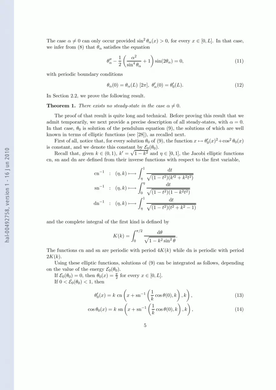
The case α 6= 0 can only occur provided sin2 θα(x) > 0, for every x ∈ [0, L]. In that case,we infer from (8) that θα satisfies the equation

θ′′α − 1

2

(α2

sin4 θα+ 1

)sin(2θα) = 0, (11)

with periodic boundary conditions

θα(0) = θα(L) [2π], θ′α(0) = θ′0(L). (12)

In Section 2.2, we prove the following result.

Theorem 1. There exists no steady-state in the case α 6= 0.

The proof of that result is quite long and technical. Before proving this result that weadmit temporarily, we next provide a precise description of all steady-states, with α = 0.In that case, θ0 is solution of the pendulum equation (9), the solutions of which are wellknown in terms of elliptic functions (see [28]), as recalled next.

First of all, notice that, for every solution θ0 of (9), the function x 7→ θ′0(x)2+cos2 θ0(x)is constant, and we denote this constant by E0(θ0).

Recall that, given k ∈ (0, 1), k′ =√

1 − k2 and η ∈ [0, 1], the Jacobi elliptic functionscn, sn and dn are defined from their inverse functions with respect to the first variable,

cn−1 : (η, k) 7−→∫ 1

η

dt√(1 − t2)(k′2 + k2t2)

sn−1 : (η, k) 7−→∫ η

0

dt√(1 − t2)(1 − k2t2)

dn−1 : (η, k) 7−→∫ 1

η

dt√(1 − t2)(t2 + k2 − 1)

and the complete integral of the first kind is defined by

K(k) =

∫ π/2

0

dθ√1 − k2 sin2 θ

.

The functions cn and sn are periodic with period 4K(k) while dn is periodic with period2K(k).

Using these elliptic functions, solutions of (9) can be integrated as follows, dependingon the value of the energy E0(θ0).

If E0(θ0) = 0, then θ0(x) = π2 for every x ∈ [0, L].

If 0 < E0(θ0) < 1, then

θ′0(x) = k cn

(x + sn−1

(1

kcos θ(0), k

), k

), (13)

cos θ0(x) = k sn

(x + sn−1

(1

kcos θ(0), k

), k

), (14)

5

hal-0

0492

758,

ver

sion

1 -

16 J

un 2

010

for every x ∈ [0, L], with E0(θ0) = k2. The period of θ0 is T = 4K(k) = 4K(√

E0(θ0)).This case corresponds to the closed curves of Figure 1.

If E0(θ0) = 1, then

θ′0(x) = 1/cosh(x + argth−1 (cos θ(0))

), (15)

cos θ0(x) = tanh(x + argth−1 (cos θ(0))

). (16)

This case corresponds to the separatrices (in bold) of the phase portrait drawn on Figure1.

If E0(θ0) > 1, then

θ′0(x) =1

kdn(x

k+ sn−1 (cos θ(0), k) , k

), (17)

cos θ0(x) = sn(x

k+ sn−1 (cos θ(0), k) , k

), (18)

for every x ∈ [0, L], with E0(θ0) = 1/k2. Moreover, θ0(x + T ) = θ0(x) + 2π for everyx ∈ [0, L] with T = 2kK(k) = 2K(1/

√E0(θ0))/

√E0(θ0). This case corresponds to the

curves located above and under the separatrices of Figure 1.

K1 0 1 2 3 4

K2

K1

1

2

Figure 1: Phase portrait of (9) (in the plane (θ, θ′))

Every steady-state must moreover satisfy the boundary conditions (10), with the periodL. These boundary conditions appear as an additional constraint to be satisfied by thesolutions above, which turns into a quantification property, as explained in the next result.

Theorem 2. Set N0 =[

L2π

], where the bracket notation stands for the integer part. Then,

there exists a family (En)16n6N0of elements of (0, 1) and a countable family (En)n∈N∗ of

elements of (1,+∞) such that, for every steady-state,

• if 0 6 E0(θ0) < 1, then E0(θ0) ∈ E1, . . . , EN0;

6

hal-0

0492

758,

ver

sion

1 -

16 J

un 2

010

• if E0(θ0) > 1, then E0(θ0) ∈ En | n ∈ N∗.

Note that, if L < 2π, there is no solution satisfying E0(θ0) < 1.

Proof. To take into account the boundary conditions (10), we have to impose that L isequal to an integer multiple of the period T of θ0. The expression of T using the ellipticfunction K has been given previously, depending on the energy E0(θ0). Recall that K isan increasing function from [0, 1) into [π/2,+∞). The graph of the period T as a functionof E0(θ0) is given on Figure 2. The conclusion follows easily.

0 1 2 3 4 5 60

2

4

6

8

10

12

Figure 2: Graph of the period T in function of E0(θ0) (case α = 0)

2.2 Proof of Theorem 1

Consider a L-periodic steady-state in the case α 6= 0. It follows from (11) that the function

x 7→ θ′α(x)2 +α2

sin2 θα(x)+ cos2 θα(x)

is constant, and we define the functional

Eα(θα) = θ′2α +α2

sin2 θα+ cos2 θα. (19)

As in the previous subsection, it is a kind of energy that is not related to the energy definedby (1). Recall that, since α 6= 0, there must hold sin θα(x) 6= 0, for every x ∈ [0, L], andhence θα(x) ∈ (pπ, (p+1)π), for some p ∈ Z. The phase portrait of (11), drawn on Figure3 is then very different of the one of the pendulum studied previously. The vertical linesθ = 0 [π] are made of singular points. The region of the phase portrait of the pendulum(Figure 1) inside the separatrices can be seen as a sort of compactification process in which

7

hal-0

0492

758,

ver

sion

1 -

16 J

un 2

010

both vertical lines θ = 0 and θ = π would join to form the separatrices. The trajectoriesthat are outside the separatrices of the phase portrait of the pendulum do not exist in thecase α 6= 0.

K1 0 1 2 3 4

K2

K1

1

2

Figure 3: Phase portrait of (11) (case α 6= 0)

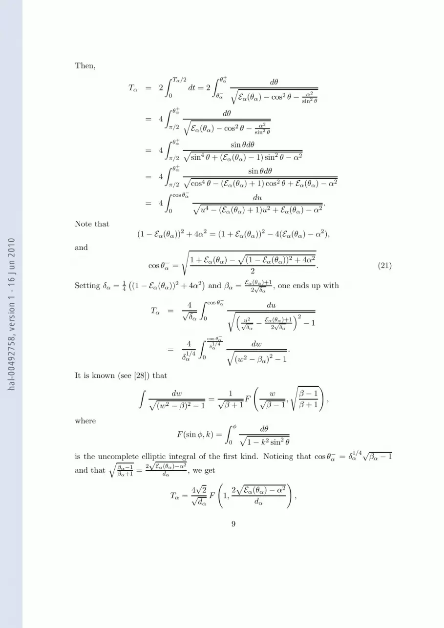
First of all, note that there must hold necessarily Eα(θα) > α2. It can be easily provedthat every solution of (11) is periodic.

Lemma 1. Let θα be a solution of (11). Then, its period is

Tα =4√

2√dα

K

(2√

Eα(θα) − α2

dα

), (20)

where dα = Eα(θα) + 1 +√

(1 − Eα(θα))2 + 4α2.

Proof. We assume that θα(x) ∈ (0, π). Denote by θ−α and θ+α the extremal values of θα(x).

They are computed by solving the equation

sin4 θ + (Eα(θα) − 1) sin2 θ − α2 = 0.

This leads to

θ−α = arcsin

√1 − Eα(θα) +

√(Eα(θα) − 1)2 + 4α2

2, θ+

α = π − θ−α .

8

hal-0

0492

758,

ver

sion

1 -

16 J

un 2

010

Then,

Tα = 2

∫ Tα/2

0dt = 2

∫ θ+α

θ−α

dθ√Eα(θα) − cos2 θ − α2

sin2 θ

= 4

∫ θ+α

π/2

dθ√Eα(θα) − cos2 θ − α2

sin2 θ

= 4

∫ θ+α

π/2

sin θdθ√sin4 θ + (Eα(θα) − 1) sin2 θ − α2

= 4

∫ θ+α

π/2

sin θdθ√cos4 θ − (Eα(θα) + 1) cos2 θ + Eα(θα) − α2

= 4

∫ cos θ−α

0

du√u4 − (Eα(θα) + 1)u2 + Eα(θα) − α2

.

Note that(1 − Eα(θα))2 + 4α2 = (1 + Eα(θα))2 − 4(Eα(θα) − α2),

and

cos θ−α =

√1 + Eα(θα) −

√(1 − Eα(θα))2 + 4α2

2. (21)

Setting δα = 14

((1 − Eα(θα))2 + 4α2

)and βα = Eα(θα)+1

2√

δα, one ends up with

Tα =4√δα

∫ cos θ−α

0

du√(u2√δα

− Eα(θα)+1

2√

δα

)2− 1

=4

δ1/4α

∫ cos θ−α

δ1/4α

0

dw√(w2 − βα)2 − 1

.

It is known (see [28]) that

∫dw√

(w2 − β)2 − 1=

1√β + 1

F

(w√

β − 1,

√β − 1

β + 1

),

where

F (sin φ, k) =

∫ φ

0

dθ√1 − k2 sin2 θ

is the uncomplete elliptic integral of the first kind. Noticing that cos θ−α = δ1/4α

√βα − 1

and that√

βα−1βα+1 =

2√

Eα(θα)−α2

dα, we get

Tα =4√

2√dα

F

(1,

2√

Eα(θα) − α2

dα

),

9

hal-0

0492

758,

ver

sion

1 -

16 J

un 2

010

with dα = Eα(θα) + 1 +√

(Eα(θα) − 1)2 + 4α2, which is the expected result.

Remark 1. For α = 0, we recover the period obtained in the previous section for trajec-tories that are inside the separatrices. Indeed, taking α = 0 in (20) leads to

T0 =4√

2√E0(θ0) + 1 + |E0(θ0) − 1|

K

(2√

E0(θ0)

E0(θ0) + 1 + |E0(θ0) − 1|

), (22)

and hence

T0 =

4K(

√E0(θ0)) if 0 6 E0(θ0) < 1,

+∞ if E0(θ0) = 1.

The function T0 defined by (22) is also defined for E0(θ0) > 1, however it differs fromthe period of trajectories of the pendulum phase portrait (see previous section) that areoutside the separatrices. This is not surprising, since these trajectories do not exist in thecase α 6= 0, as explained formerly.

Considering Tα as a function of E0(θ0), this function is smooth on (α2,+∞), for α 6= 0,and, setting E0(θ0) = α2 + η, a lengthy computation shows that

T ′α(α2 + η) =

4√

2

(f1(η))3/2

(f ′1(η)

2K

(2√

η

f1(η)

)+

1√ηK ′(

2√

η

f1(η)

)

− f ′1(η)K

(2√

η

f1(η)

)),

for every η > 0, where f1(η) = η+α2 +1+√

(η + α2 − 1)2 + 4α2, and K ′(k) = − 1kK(k)+

1k K(k), with

K(k) =

∫ π/2

0

dθ

(1 − k2 sin2 θ)3/2.

Moreover,

T ′α(α2 + η) ∼

η→0

π(1 − 2α2)

2(α2 + 1)5/2, (23)

andT ′

α(α2 + η) ∼η→+∞

− π

η3/2. (24)

A tedious but straightforward study leads to the following result, describing the mono-tonicity properties of that function.

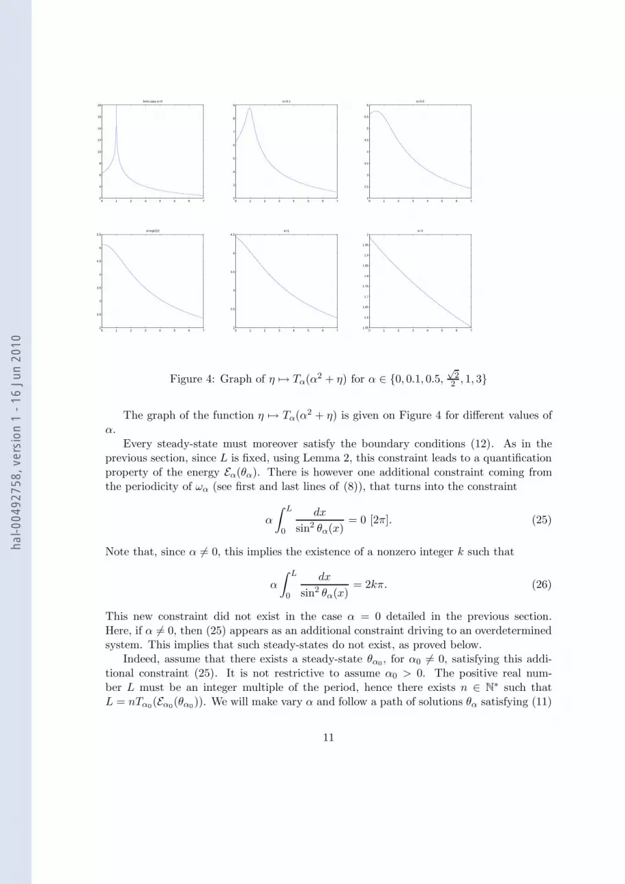
Lemma 2. For every α ∈ (0,√

22 ), there exists E∗

α ∈ (α2, 1 + α2) such that the functionE0(θ0) 7→ Tα(E0(θ0)) is increasing on (α2, E∗

α) and decreasing on (E∗α,+∞). Moreover,

Tα(E∗α) → +∞ and E∗

α → 1 whenever α → 0.

For every α >

√2

2 , the function E0(θ0) 7→ Tα(E0(θ0)) is decreasing on (α2,+∞).Moreover, for every α > 0, Tα(E0(θ0)) → 0 whenever E0(θ0) → +∞.

10

hal-0

0492

758,

ver

sion

1 -

16 J

un 2

010

0 1 2 3 4 5 6 72

4

6

8

10

12

14

16

18limit case α=0

0 1 2 3 4 5 6 72

3

4

5

6

7

8

9α=0.1

0 1 2 3 4 5 6 72

2.5

3

3.5

4

4.5

5

5.5

6α=0.5

0 1 2 3 4 5 6 72

2.5

3

3.5

4

4.5

5

5.5α=sqrt2/2

0 1 2 3 4 5 6 72

2.5

3

3.5

4

4.5α=1

0 1 2 3 4 5 6 71.55

1.6

1.65

1.7

1.75

1.8

1.85

1.9

1.95

2α=3

Figure 4: Graph of η 7→ Tα(α2 + η) for α ∈ 0, 0.1, 0.5,√

22 , 1, 3

The graph of the function η 7→ Tα(α2 + η) is given on Figure 4 for different values ofα.

Every steady-state must moreover satisfy the boundary conditions (12). As in theprevious section, since L is fixed, using Lemma 2, this constraint leads to a quantificationproperty of the energy Eα(θα). There is however one additional constraint coming fromthe periodicity of ωα (see first and last lines of (8)), that turns into the constraint

α

∫ L

0

dx

sin2 θα(x)= 0 [2π]. (25)

Note that, since α 6= 0, this implies the existence of a nonzero integer k such that

α

∫ L

0

dx

sin2 θα(x)= 2kπ. (26)

This new constraint did not exist in the case α = 0 detailed in the previous section.Here, if α 6= 0, then (25) appears as an additional constraint driving to an overdeterminedsystem. This implies that such steady-states do not exist, as proved below.

Indeed, assume that there exists a steady-state θα0, for α0 6= 0, satisfying this addi-

tional constraint (25). It is not restrictive to assume α0 > 0. The positive real num-ber L must be an integer multiple of the period, hence there exists n ∈ N

∗ such thatL = nTα0

(Eα0(θα0

)). We will make vary α and follow a path of solutions θα satisfying (11)

11

hal-0

0492

758,

ver

sion

1 -

16 J

un 2

010

and (12), such that θα = θα0for α = α0, in order to raise some contradiction for some

well chosen value of α.At this step, we have to distinguish between two cases.

Case 0 < α0 <√

2/2. Standard arguments for ordinary differential equations show thatwe can decrease α (at least in a neighborhood of α0) and follow a path of solutions θα

satisfying (11) and (12), such that θα = θα0for α = α0. Using Lemma 2 and in particular

the fact that the maximum Tα(E∗α) tends to +∞, it is clear that it is possible to make α

decrease down to 0 and to follow a path such that Eα(θα) < 1. Moreover, combining theexpression of T0 and the formula (21), it is clear that this path shares the following crucialproperty: there exists ε > 0 such that, for every α ∈ (0, α0), there holds ε 6 θα(x) 6 π−ε.This implies that there exists M > 0 such that, for every α ∈ (0, α0),

∫ L

0

dx

sin2 θα(x)6 M.

Besides, using (26) and the continuity with respect to α, there must hold

α

∫ L

0

dx

sin2 θα(x)= 2kπ,

for every α ∈ (0, α0). We obtain a contradiction for α small enough.

Case α0 >√

2/2. Similarly, standard arguments for ordinary differential equations showthat we can increase α (at least in a neighborhood of α0) and follow a path of solutionsθα satisfying (11) and (12), such that θα = θα0

for α = α0. Using Lemma 1, there holds

Tα(α2) =2π√

α2 + 1.

Hence, it is possible to increase α up to a value α1 satisfying

Tα1(α2

1) = L/n.

This implies Eα1(θα1

) = α21. On the phase portrait of Figure 3, this corresponds to following

trajectories shrinking to the center point θ = π/2, θ′ = 0. The value α1 is characterizedby

2π√α2

1 + 1=

L

n. (27)

For α < α1, α close to α1, we set Eα(θα) = α2 + η, with η > 0 small. In what follows, weare going to expand the solution θα at the first order and express, at the first order, theconstraints (26) and Tα(α2 + η) = L/n, in order to raise a contradiction.

Using (11) and (19), we get, at the first order,

θ(x) − π

2∼√

η

1 + α2sin(

√1 + α2 x),

12

hal-0

0492

758,

ver

sion

1 -

16 J

un 2

010

for η > 0 small and α1 − α > 0 small. Using (11), we get

α

∫ L

0

dx

cos2(√

η1+α2 sin

(√1 + α2 x

)) = 2kπ, (28)

and, using (23), we infer from the constraint Tα(α2 + η) = L/n that

2π√α2 + 1

+ ηπ

2

1 − 2α2

(1 + α2)5/2=

L

n, (29)

for η > 0 small and α1 − α > 0 small. A simple asymptotic computation of the integralterm of (28) leads to

αL +αη

4(1 + α2)3/2

(2√

1 + α2L − sin(2√

1 + α2L))

= 2kπ.

Combining that equation with (29) yields

αL +α

2π

α2 + 1

1 − 2α2

(L

n− 2π√

α2 + 1

)(2√

1 + α2L − sin(2√

1 + α2L))

= 2kπ,

for every α < α1 sufficiently close to α1. This is a contradiction.The proof of Theorem 1 is complete.

3 Stability properties of the steady-states

In order to investigate the stability properties of the steady-states, we compute the lin-earized system around a given steady-state and study its spectral properties. In whatfollows, define the spaces

H1per(0, L; R3) = u ∈ H1(0, L; R3) | u(0) = u(L),

H2per(0, L; R3) = u ∈ H2(0, L; R3) | u(0) = u(L) and u′(0) = u′(L).

Endowed respectively with the usual H1 and H2 inner product, these are Hilbertian spaces.Let M0 be a steady-state. The results of the previous section show that, in the spherical

coordinates (θ, ω) that have been used, the component ω is constant. Clearly, the equation(4) is invariant with respect to rotations around the axis Re1. Then, up to a rotation ofangle ω around the axis Re1, we assume that

M0(x) =

cos θ(x)sin θ(x)

0

,

where θ is solution of (9), (10) as described in Section 2. In Section 3.1, we compute thelinearized system around this steady-state. The operator underlying this linearized systemis a matrix of one-dimensional operators, one of which, denoted A, plays an important role.

13

hal-0

0492

758,

ver

sion

1 -

16 J

un 2

010

We study in details the spectral properties of A in Section 3.2. Based on this preliminarystudy, we investigate in Section 3.3 the stability properties of the steady-state M0. Noticethat the linearized system is as well invariant with respect to rotations around the axisRe1, and hence these results hold for every L-periodic steady-state. Finally, Section 3.4 isdevoted to prove that the eigenvalues of the linearized system are simple except for certaindiscrete values of L.

3.1 Linearization of (4) around a steady-state

Let u be a solution of (4). As in [5], we complete M0 into the mobile frame (M0(x),M1(x),M2),where M1 and M2 are defined by

M1(x) =

− sin θ(x)cos θ(x)

0

, M2 =

001

.

Considering u as a perturbation of the steady-state M0, since |u(t, x)| = 1 pointwisely, wedecompose u : R+ × R −→ S

2 ⊂ R3 in the mobile frame as

u(t, x) =√

1 − r21(t, x) − r2

2(t, x)M0(x) + r1(t, x)M1(x) + r2(t, x)M2. (30)

Easy but lengthy computations show that u is solution of (4) if and only if r =

(r1

r2

)

satisfies∂r

∂t= Lr + R(x, r, rx, rxx), (31)

where

R(x, r, rx, rxx) = G(r)rxx + H1(x, r)rx + H2(r)(rx, rx),

and

• L =

(A + Id A + E0(θ)Id

−(A + Id) A + E0(θ)Id

)with A = ∂2

xx − 2 cos2 θ Id defined on the domain

D(A) = H2per(0, L),

• G(r) is the matrix defined by

G(r) =

r1r2√1−|r|2

r22√

1−|r|2+√

1 − |r|2 − 1

− r21√

1−|r|2−√

1 − |r|2 + 1 − r1r2√1−|r|2

,

• H1(x, r) is the matrix defined by

H1(x, r) =2θ′(x)√1 − |r|2

(r2

√1 − |r|2 − r1r

22 −r2(1 − r2

1)

r2(1 − r22)

√1 − |r|2r2 + r1r

22

),

14

hal-0

0492

758,

ver

sion

1 -

16 J

un 2

010

• H2(r) is the quadratic form on R2 defined by

H2(r)(X,X) =(1 − |r|2)X⊤X + (r⊤X)2

(1 − |r|)3/2

(√1 − |r|2r1 + r2√1 − |r|2r2 − r1

),

with the estimates

G(r) = O(|r|2),H1(r) = O(|r|),H2(r) = O(|r|).

It is not difficult to prove that there exists a constant C > 0 such that, if |r|2 612 , then,

there holds for every x ∈ R, for every (p, q) ∈ (R2)2,

|R(x, r, p, q)| 6 C(|r|2|q| + |r|.|p| + |r|.|p|2).

This a priori estimate shows that R(x, r, rx, rxx) is a remainder term in (31).

3.2 Spectral study of the operator A = ∂2xx − 2 cos2 θ Id

In this section, we derive spectral properties of the operator A appearing in the expressionof the linearized operator L, which will be useful for the stability analysis of Section 3.3.The domain of A is H2

per(0, L; R3), but of course it is equivalent to study A on the domainD(A) = H2

per(0, L; R) (denoted shortly H2per(0, L)).

Every eigenpair (λ, u) of A must satisfy

u′′ − 2 cos2 θ u = λu,

u(0) = u(L), u′(0) = u′(L).

This is a particular case of Sturm-Liouville type problems with real coupled self-adjointboundary conditions (see [23, 24, 25]). The following result provides some spectral prop-erties of A.

Proposition 1. The operator A, defined on D(A) = H2per(0, L), is selfadjoint in L2(0, L)

and there exists a hilbertian basis (ek)k∈N of L2(0, L), consisting of eigenfunctions of A,associated with real eigenvalues λk that are at most double, with

−∞ < · · · 6 λk 6 · · · 6 λ1 6 λ0, (32)

and λk → −∞ as k → +∞. Moreover,

• there cannot be two successive equalities in (32);

• the eigenfunction e0 vanishes 0 or 1 time on [0, L];

• the eigenfunction ek vanishes k − 1 or k or k + 1 times on [0, L].

15

hal-0

0492

758,

ver

sion

1 -

16 J

un 2

010

Remark 2. A simple computation shows that

A sin θ = −E0(θ) sin θ,

Aθ′ = −θ′,

A cos θ = −(1 + E0(θ)) cos θ.

Hence, sin θ, θ′ and cos θ are eigenfunctions of A associated respectively with the eigen-values −E0(θ),−1,−(1 + E0(θ)). We are not able to exhibit nor compute explicitly someother eigenelements of A.

Note that, if the steady-state under consideration satisfies E0(θ) > 1 (that is, thecorresponding trajectory on the phase portrait of Figure 1 is outside the separatrices),then the function θ′ does not vanish, and it follows from Proposition 1 that λ0 = −1, thatis, −1 is the largest eigenvalue of A, and e0 = θ′.

If the steady-state under consideration satisfies E0(θ) < 1 (that is, the correspondingtrajectory on the phase portrait of Figure 1 is inside the separatrices), then the functionsin θ does not vanish, and it follows from Proposition 1 that λ0 = −E0(θ), that is, −E0(θ)is the largest eigenvalue of A, and e0 = sin θ.

In the particular case θ = π/2 (corresponding to E0(θ) = 0), one has θ′ = 0 andcos θ = 0 and thus they are not eigenfunctions. In that case, λ0 = 0, and e0 = 1. By theway, all eigenvalues can be easily computed.

Proof. We first prove that the operator A is diagonalisable. Consider the ordinary differ-ential equation with boundary conditions

− u′′ + (2 cos2 θ + 1)u = f,

u(0) = u(L), u′(0) = u′(L).(33)

This problem is equivalent to the problem of determining u ∈ H2per(0, L) such that b(u, v) =

g(v) for every v ∈ H1per(0, L), where the bilinear form b and the linear form g are defined

by

b(u, v) =

∫ L

0u′(x)v′(x)dx +

∫ L

0(2 cos2 θ(x) + 1)u(x)v(x)dx,

g(v) =

∫ L

0f(x)v(x)dx.

Moreover, it is clear that

‖u‖2H1(0,L) 6 b(u, u),

|b(u, v)| 6 4‖u‖H1(0,L)‖v‖H1(0,L),

|g(v)| 6 ‖f‖L2(0,L)‖v‖H1(0,L),

for all u, v ∈ H1per(0, L). This implies that b is continuous and coercive, and g is continuous.

Lax-Milgram’s Theorem then implies the existence of a unique weak solution in H1per(0, L),

and it is easy to prove that this solution is strong and belongs to H2per(0, L), using a

standard bootstrap argument.

16

hal-0

0492

758,

ver

sion

1 -

16 J

un 2

010

It is then possible to define the linear operator

F : L2(0, L) −→ L2(0, L)f 7−→ u

where u is the unique solution of (33).The operator F is self-adjoint. Indeed, let f1, f2 ∈ L2(0, L) and set u1 = Ff1 and

u2 = Ff2. Then,

〈Ff1, f2〉L2(0,L) = 〈u1, f2〉L2(0,L) = b(u1, u2) = 〈f1, Ff2〉L2(0,L).

The operator F is compact. Indeed, let u = Ff , for f ∈ L2(0, L). Then,

‖u‖2H1(0,L) 6 b(u, u) 6 ‖f‖L2(0,L)‖u‖H1(0,L),

and hence ‖u‖H1(0,L) = ‖Ff‖H1(0,L) 6 ‖f‖L2(0,L). Since the imbedding of H1(0, L) intoL2(0, L) is compact, it follows that the operator F is compact.

Since F is compact and selfadjoint, it follows that the operator A is diagonalisablewith real eigenvalues satisfying (32). The eigenvalues λk are at most double because theassociated eigenfunctions are solutions of a linear ordinary differential equation of ordertwo. There cannot be two successive equalities in (32) because the eigenproblem associatedto λn has exactly two linearly independent solutions. The two last assertions concerningthe zero properties of the eigenfunctions follow from [25].

3.3 Stability properties of the steady-states

Consider the linear system

∂z

∂t= Lz

z(t, 0) = z(t, L), z′(t, 0) = z′(t, L),(34)

obtained in Section 3.1 by linearizing the Landau-Lifschitz equation (4) around the steadystate M0. For every k > 0, set

zk(t) = 〈z(t, ·), ek〉L2(0,L),

where (ek)k∈N is the hilbertian basis of eigenfunctions of A introduced in Lemma 1. Then,(34)) is equivalent to the series of 2 × 2 linear systems

∂zk

∂t= Lkz,

zk(0) = zk(L), z′k(0) = z′k(L),

for every k ∈ N, where

Lk =

(λk + 1 λk + E0(θ)

−(λk + 1) λk + E0(θ)

).

Recall that a matrix is said Hurwitzian whenever all its eigenvalues have their real partlower than 0. One has the following result.

17

hal-0

0492

758,

ver

sion

1 -

16 J

un 2

010

Lemma 3. For every k ∈ N, the matrix Lk is Hurwitzian if and only if λk < min(−1,−E0(θ)).

Proof. Set m = min(−1,−E0(θ)) and M = max(−1,−E0(θ)). The matrix Lk is Hurwitzianif and only if its determinant is positive and its trace is negative, that is, if and only if(λk + 1)(λk + E0(θ)) > 0 and 2λk + 1 + E0(θ) < 0. The trace condition yields λk < m+M

2 ,and the determinant condition yields λk < m or λk > M . The conclusion follows.

To establish spectral properties of the steady-states, we distinguish between four cases,depending on value of the energy E0(θ) of the steady-state under consideration.

3.3.1 Case E0(θ) = 0

In this case, there holds θ = π/2 and θ′ = 0. Hence, A = ∂2xx, and in that case all

eigenvalues of A are explicitly computed as λk = −(

2kπL

)2, for k ∈ N. Unstable modes

correspond to the eigenvalues λk satisfying λk > −1, and hence there are exactly[

L2π

]+ 1

unstable modes whenever L2π is not integer, and L

2π whenever it is an integer. In particular,there is always at least one unstable mode, corresponding to the eigenvalue 0 and theeigenfunction 1.

3.3.2 Case E0(θ) ∈ (0, 1)

This case corresponds to periodic trajectories of the pendulum phase portrait (see Figure1) that are inside the separatrices.

Lemma 4. The operator A + E0(θ)Id admits the factorization

A + E0(θ)Id = −ℓ∗ℓ,

where the operator ℓ is defined by ℓ = ∂x − θ′cotanθ Id on the domain D(ℓ) = H1per(0, L).

As a consequence, the largest eigenvalue of A is λ0 = −E0(θ).

Proof. First of all, note that sin θ(x) 6= 0 for every x ∈ [0, L]. Indeed, the identityθ′2(x)+cos2 θ(x) = E0(θ) < 1 yields cos2 θ(x) < 1 for every x ∈ [0, L] and hence sin θ(x) 6=0. Defining ℓ as in the statement of Lemma 4, there holds ℓ∗ = −∂x − θ′cotan θ Id,with D(ℓ∗) = D(ℓ) = H1

per(0, L). One has H2per(0, L) = D(A + E0(θ)Id) ⊂ D(ℓ) and

ℓ(D(A + E0(θ)Id)) ⊂ D(ℓ∗), and one computes

−ℓ∗ℓ = −(−∂x − θ′cotanθ Id) (∂x − θ′ cotan θ Id)

= ∂2xx − θ′′ cotanθ Id +

θ′2

sin2 θId − θ′cotanθ ∂x

+θ′cotanθ ∂x + θ′2cotan 2θ Id

= ∂2xx + (E0(θ) − 2 cos2 θ)Id,

since θ′2 = E0(θ)− cos2 θ. It follows from this factorization that the operator A + E0(θ)Idis nonpositive, and hence, since −E0(θ)Id is an eigenvalue of A, λ0 = −E0(θ).

18

hal-0

0492

758,

ver

sion

1 -

16 J

un 2

010

From Lemma 3, the matrix Lk is Hurwitzian if and only if λk < −1. Then, thereis always a finite number of unstable modes, corresponding to the eigenvalues λk suchthat −1 < λk 6 −E0(θ). In particular, using Remark 2, e0 = sin θ is an unstable modeassociated with λ0 = −E0(θ). Moreover, if L is large, then, when solving T = L/n as in theproof of Theorem 2, the steady-state may be such that the integer n may be large (notethat n ∈ 1, . . . , N0 with N0 = [ L

2π ]). On the phase portrait of the pendulum (Figure 1),this means that, for this situation, the corresponding trajectory turns n times around thecenter point θ = π/2, θ′ = 0 on the interval [0, L], and hence θ′ vanishes 2n times; it thenfollows from Proposition 1 that θ′ is the kth eigenfunction, with k ∈ 2n − 1, 2n, 2n + 1.Therefore, in that situation, since the eigenvalue −1 is at most double, there exist at least2n − 1 and at most 2n + 1 unstable modes.

The eigenvalue −1 (associated at least with the eigenfunction θ′, from Remark 2),corresponds to a central manifold for the nonlinear system (4) around the steady-stateM0.

All other eigenvalues λk, such that λk < −1, correspond to stable modes (in infinitenumber).

Notice that, since n 6 N0, for every L-periodic steady-state such that E0(θ) ∈ (0, 1),there are at most 2[ L

2π ] + 1 unstable modes.

3.3.3 Case E0(θ) = 1

In this case, there must hold either θ = θ′ = 0, or θ = π and θ′ = 0. Hence, cos θis constant, equal to 1 or −1. Since it does not vanish, it follows from Proposition 1and Remark 2 that λ0 = −2. Actually, in that case, one has A = ∂xx − 2Id, and alleigenvalues can be easily computed. The corresponding steady-state is M0 = (1, 0, 0)T , orM0 = (−1, 0, 0)T (the resulting magnetic field is constant, tangent to the nanowire). It islocally asymptotically stable for the system (4).

3.3.4 Case E0(θ) > 1

This case corresponds to periodic trajectories of the pendulum phase portrait (see Figure1) that are outside the separatrices.

Note that, in that case, the factorization of Lemma 4 does not hold. This is due tothe fact that sin θ vanishes.

From Lemma 3, the matrix Lk is Hurwitzian if and only if λk < −E0(θ). The situationis similar to the case E0(θ) ∈ (0, 1), except that the roles of −1 and −E0(θ) are exchanged.More precisely, there is always a finite number of unstable modes, corresponding to theeigenvalues λk such that −E0(θ) < λk 6 −1. In particular, using Remark 2, e0 = θ′ is anunstable mode associated with λ0 = −1. Moreover, as previously, when solving T = L/nas in the proof of Theorem 2, the steady-state may be such that the integer n may belarge (and contrarily to the case E0(θ) ∈ (0, 1), there exist steady-states such that n isarbitrarily large). This means that, for this situation, sin θ vanishes a 2n times; it thenfollows from Proposition 1 that sin θ is the kth eigenfunction, with k ∈ 2n−1, 2n, 2n+1.Therefore, in that situation, since −E0(θ) is at most double, there exist at least 2n−1 and

19

hal-0

0492

758,

ver

sion

1 -

16 J

un 2

010

at most 2n + 1 unstable modes.Notice that, for every integer p, there exists a L-periodic steady-state for which E0(θ) >

1, such that the corresponding operator A admits at least p unstable modes.

3.4 On the simplicity of the eigenvalues of A

In this section, we investigate the simple character of the eigenvalues of A seen as functionsof L. This question may be important in view of potential controllability issues.

Theorem 3. For every L-periodic steady-state associated with a function θ, every eigen-value of the corresponding operator A is simple except for certain isolated values of L.

Remark 3. Since there is a countable number of eigenvalues, the theorem implies thatall eigenvalues of A are simple except for a countable set of values of L.

Proof. Consider a steady-state associated with the L-periodic function θ. To derive thetheorem, we distinguish between three cases. The first case is when E0(θ) < 1, that is, thecorresponding trajectory on the phase portrait of Figure 1 is inside the separatrices. Thesecond case is when E0(θ) = 1, and in that case the eigenvalues are explicitly computedand the conclusion is immediate. The third case, E0(θ) > 1, is more difficult to treat; itcorresponds on the phase portrait of Figure 1 to a trajectory outside the separatrices.

First case: E0(θ) < 1. Assume that the period is such that 4K(k) = L/n, for some n ∈N∗ (see Section 2). The idea is to decrease continuously L and to follow the corresponding

continuous path of associated functions θL. The corresponding eigenvalues of A (nowrather denoted AL, to point out the dependence on L) depend continuously on L. Thisassertion indeed follows from a standard result of continuous dependence of eigenvalues(see e.g. [24]). It is possible to make L decrease down to 2nπ. This corresponds onthe phase portrait of Figure 1 to make the trajectory (θL, θ′L) shrink to the center pointθ = π/2, θ′ = 0. For L1 = 2nπ, the constraint 4K(k) = L/n indeed implies that k = 0,E0(θL1

) = 0, and θL1= π/2, θ′L1

= 0. Then, for L = L1, there holds AL1= ∂xx; in that

case, and as mentioned formerly, all eigenvalues are computed explicitly as λk = −(

2kπL1

)2,

for every k ∈ N, and moreover all eigenvalues are simple. It follows from [24, Theorem 3.1and Lemma 3.2] that all eigenvalues of the operator AL are simple, for every L close toL1, with L > L1. We have thus proved the following lemma.

Lemma 5. There exists ε > 0 such that all eigenvalues of the operator AL are simple, forevery L ∈ [L1, L1 + ε).

Our aim is now to use an analyticity argument in order to prove the exceptionalcharacter of double eigenvalues. First of all, recall that, from Rellich’s Theorem (see [31]or [22]), since the spectrum of the operator A is separated (see Proposition 1), everyeigenvalue of AL is an analytic function of L.

20

hal-0

0492

758,

ver

sion

1 -

16 J

un 2

010

Let λ(L) be an eigenvalue of AL, associated to an eigenfunction uL. This means thatthe couple (λ(L), uL) is solution of the boundary value problem

u′′ − cos2 θL u = λu,

u(0) = u(L), u′(0) = u′(L),(35)

which is equivalent, setting Y = (u, u′)T , to the boundary value problem

Y ′ =

(0 1

λ + cos2 θL 0

)Y, (36)

Y (0) = Y (L). (37)

Moreover, the multiplicity of λ(L) is the dimension of the associated space of solutionsof (36)-(37). For every real number λ, denote by Φ(·, λ) be the resolvent of (36), withΦ(0, λ) = I2, where I2 is the 2 × 2 identity matrix. Note that Φ is analytic. Using theresolvent, every solution Y (·) of (36) is written as Y (·) = Φ(·, λ)Y (0), and every solution(λ, Y (·)) of the boundary value problem (36)-(37) must satisfy (Φ(L, λ)− I2)Y (0) = 0 andthus δ(λ) = 0, with

δ(λ) = det(Φ(L, λ) − I2). (38)

Note that the function λ 7→ δ(λ) defined by (38) is an analytic function. It is usually calledthe characteristic function of the eigenvalue problem (35), and the equation δ(λ) = 0 iscalled transcendental equation (see [24]). Its zeros are exactly the eigenvalues of AL.Moreover, λ is a double eigenvalue of AL if and only if the space of solutions of (36)-(37)is of dimension 2, and this is equivalent to Φ(L, λ) − I2 = 0. We sum up these results inthe following lemma.

Lemma 6. Denoting by λk(L) the kth eigenvalue of AL, the function L 7→ λk(L) isanalytic, for every k ∈ N. The eigenvalues of AL are exactly the zeros of the analyticfunction δ(·) defined by (38). Moreover, λ is a double eigenvalue of AL if and only ifΦ(L, λ) = I2.

Let k an integer. From Lemma 6, the eigenvalue λk(L) is double if and only ifΦ(L, λk(L)) = I2. By analyticity, either this equality may only occur for isolated valuesof L, or this equality holds for every L > L1. Lemma 5 implies that the latter possibilitydoes not happen. Therefore, every eigenvalue of AL is simple except for isolated values ofL.

Second case: E0(θ) = 1. In this case, as mentioned formerly, there must hold eitherθ = θ′ = 0, or θ = π and θ′ = 0. It follows that A = ∂xx − 2Id, and all eigenvalues can be

explicitly computed as λk = −2 −(

2kπL

)2, for every k ∈ N, and moreover all eigenvalues

are simple, for every value of L.

21

hal-0

0492

758,

ver

sion

1 -

16 J

un 2

010

Third case: E0(θ) > 1. This case is more difficult to treat than the case E0(θ) < 1.Assume that the period is such that 2kK(k)=L/n, for some n ∈ N

∗ (see Section 2). In afirst step, we proceed similarly as in the case E0(θ) < 1, and follow a path a solutions θL,making L decrease down to a small value L1, to be chosen later. Notice that, observingFigure 2, it follows that E0(θL1

) is large. On the phase portrait of Figure 1, this correspondsto considering a trajectory that is far from the separatrices.

Lemma 7. If L1 is small enough, then all eigenvalues of the operator AL1, defined on

D(AL1) = H2

per(0, L1), are simple.

Proof. In order to prove this lemma, we will consider the same differential operator ∂xx −2 cos2 θL1

Id on different domains. For every p ∈ N∗, denote by AL1,p the differential

operator ∂xx − 2 cos2 θL1Id defined on the domain D(AL1,p) = H2

per(0, pL1). Note thatAL1,1 coincides with AL1

.In particular, this means that we consider the function θL1

on the interval [0, pL1]. Ofcourse, its energy E0(θL1

) is still the same, for every p ∈ N∗.

It is obvious that, if λ is an eigenvalue of AL1,1 associated with an eigenvector u, thenλ is an eigenvalue of AL1,p associated with the same eigenvector u, for every p ∈ N

∗;moreover, if λ is simple for AL1,p then it is simple as well for AL1,1. This fact is crucial inour argument.

For L1 small enough, as mentioned formerly E0(θL1) is large, and it follows from the

relation θ′2L1

+ cos2 θL1= E0(θL1

) that θ′L(x) =√E0(θL1

) + o(1), where the term o(1)denotes a negligible term with respect to 1 whenever E0(θL1

) tends to +∞, and then,θL(x) = (

√E0(θL1

)+o(1))x. Choosing the integer p large enough implies that the functionx 7→ 2 cos2(θL1

(x)) is close to the constant function 1 in L1(0, pL1). Therefore, the operatorAL1,p is close, in this precise L1 sense, to the operator ∂xx−Id on the domain H2

per(0, pL1).Clearly, all eigenvalues of the latter operator are simple, and it follows from [24, Theorem3.1 and Lemma 3.2] that all eigenvalues of the operator AL1,p are simple as well.

Therefore, all eigenvalues of the operator AL1,1 are simple. This ends the proof of thelemma.

To derive the theorem in that third case, we then combine the result of Lemma 7 withthe analyticity arguments of the first case. The result follows.

References

[1] F. Alouges. A new finite element scheme for Landau-Lifshitz equations. DiscreteContin. Dyn. Syst. Ser. S 1 (2008), no. 2, 187–196.

[2] F. Alouges, K. Beauchard. Magnetization switching on small ferromagnetic ellipsoidalsamples. ESAIM Control Optim. Calc. Var. 15 (2009), no. 3, 676–711.

[3] F. Alouges, A. Soyeur. On global weak solutions for Landau-Lifshitz equations: ex-istence and nonuniqueness. Nonlinear Anal. 18 (1992), 1070–1084.

[4] F. Brown. Micromagnetics. Wiley, New York, 1963.

22

hal-0

0492

758,

ver

sion

1 -

16 J

un 2

010

[5] G. Carbou, S. Labbe. Stability for walls in ferromagnetic nanowire. Numerical math-ematics and advanced applications, 539–546. Springer, Berlin, 2006.

[6] G. Carbou, S. Labbe. Stabilization of walls for nanowires of finite length. PreprintHal (2009).

[7] G. Carbou, S. Labbe, E. Trelat. Control of travelling walls in a ferromagneticnanowire. Discrete Contin. Dyn. Syst. Ser. S 1 (2008), no. 1, 51–59.

[8] G. Carbou, S. Labbe, E. Trelat. Smooth control of nanowires by means of a magneticfield. Comm. Pure Appl. Anal. 8 (2009), no. 3, 871–879.

[9] G. Carbou, P. Fabrie. Regular solutions for Landau-Lifschitz equation in R3. Com-

mun. Appl. Anal. 5 (2001), no. 1, 17–30.

[10] G. Carbou, P. Fabrie, O. Gues. On the ferromagnetism equations in the non staticcase. Commun. Pure Appl. Anal. 3 (2004), no. 3, 367–393.

[11] A. De Simone. Energy minimizers for large ferromagnetic bodies. Arch. RationalMech. Anal. 125 (1993), no. 2, 99–143.

[12] A. De Simone, H. Knupfer, F. Otto. 2−d stability of the Neel wall. Calc. Var. PartialDifferential Equations 27 (2006), 233–253.

[13] A. De Simone, R. Kohn, S. Muller, F. Otto. Two-dimensional modelling of softferromagnetic films. R. Soc. Lond. Proc. Ser. A Math. Phys. Eng. Sci. 457 (2001),no. 2016, 2983–2991.

[14] A. De Simone, R. Kohn, S. Muller, F. Otto. A reduced theory for thin-film micro-magnetics. Comm. Pure Appl. Math. 55 (2002), no. 11, 1408–1460.

[15] A. De Simone, R. Kohn, S. Muller, F. Otto. Recent analytical developments inmicromagnetics, The Science of Hysteresis, G. Bertotti and I. Mayergoyz, Eds., vol.2., Academic Press (2006), chap. 4, 269–381.

[16] H. Haddar, P. Joly. Stability of thin layer approximation of electromagnetic wavesscattering by linear and nonlinear coatings. J. Comput. Appl. Math. 143 (2002),201–236.

[17] L. Halpern, S. Labbe. La theorie du micromagnetisme. Modelisation et simulationdu comportement des materiaux magnetiques. Matapli 66 (2001), 77–92.

[18] A. Hubert, R. Schafer. Magnetic domains: the analysis of magnetic microstructures.Springer-Verlag, 2000.

[19] R. Ignat, B. Merlet. Lower bound for the energy of Bloch Walls. To appear in Arch.Rat. Mech. Anal.

[20] R. Ignat, F. Otto. A compactness result in thin-film micromagnetics and the opti-mality of the Neel wall. J. Eur. Math. Soc. 10 (2008), no. 4, 909–956.

23

hal-0

0492

758,

ver

sion

1 -

16 J

un 2

010

[21] J. L. Joly, G. Metivier, J. Rauch. Global solutions to Maxwell equations in a ferro-magnetic medium. Ann. Henri Poincare 1 (2000), no. 2, 307–340.

[22] T. Kato. Perturbation theory for linear operators. Classics in Mathematics. Springer-Verlag, Berlin, 1995. Reprint of the 1980 edition.

[23] Q. Kong, A. Zettl. Dependence of eigenvalues of Sturm-Liouville problems on theboundary. J. Diff. Equations 126 (1996), no. 2, 389–407.

[24] Q. Kong, A. Zettl. Eigenvalues of regular Sturm-Liouville problems. J. Diff. Equations131 (1996), no. 1, 1–19.

[25] Q. Kong, H. Wu, A. Zettl. Dependence of the nth Sturm-Liouville eigenvalue on theproblem. J. Diff. Equations 156 (1999), no. 2, 328–354.

[26] S. Labbe. Fast computation for large magnetostatic systems adapted for micromag-netism. SIAM J. Sci. Comput. 26 (2005), no. 6, 2160–2175.

[27] L. Landau and E. Lifshitz. ”Electrodynamics of continuous media”, Course of the-oretical Physics, Vol. 8. Pergamon Press, Oxford-London-New York-Paris; Addison-Wesley Publishing Co., Inc., Reading, Mass, 1960. Translated from the russian byJ.B. Sykes and J.S. Bell.

[28] D. F. Lawden. Elliptic functions and applications. Springer Verlag, New York, 1989.

[29] S. Parkin et al. Magnetic domain-wall racetrack memory. Science 320 (2008), 190–194.

[30] S. Parkin et al. Magnetically engineered spintronic sensors and memory. Proceedingsof IEEE, vol. 91, no. 5 (2003), 661–680.

[31] M. Reed, B. Simon. Methods of modern mathematical physics. IV. Analysis of oper-ators. Academic Press, New York, 1978.

[32] D. Sanchez. Behaviour of the Landau-Lifshitz equation in a periodic thin layer.Asymptot. Anal. 41 (2005), no. 1, 41–69.

[33] K. Santugini-Repiquet, Modelization of a split in a ferromagnetic body by an equiv-alent boundary condition. Asymptot. Anal. 47 (2006), no. 3-4, 227–259 (Part I),261–290 (Part II).

[34] A. Visintin. On Landau-Lifshitz equations for ferromagnetism. Japan J. Appl. Math.2 (1985), no. 1, 69–84.

24

hal-0

0492

758,

ver

sion

1 -

16 J

un 2

010