Article

Stability Control for Electric Vehicles with FourIn-Wheel-Motors Based on Sideslip Angle

Kun Yang 1,* , Danxiu Dong 1, Chao Ma 1, Zhaoxian Tian 2, Yile Chang 1 and Ge Wang 1

�����������������

Citation: Yang, K.; Dong, D.; Ma, C.;

Tian, Z.; Chang, Y.; Wang, G. Stability

Control for Electric Vehicles with

Four In-Wheel-Motors Based on

Sideslip Angle. World Electr. Veh. J.

2021, 12, 42. https://doi.org/

10.3390/wevj12010042

Received: 6 December 2020

Accepted: 8 March 2021

Published: 12 March 2021

Publisher’s Note: MDPI stays neutral

with regard to jurisdictional claims in

published maps and institutional affil-

iations.

Copyright: © 2021 by the authors.

Licensee MDPI, Basel, Switzerland.

This article is an open access article

distributed under the terms and

conditions of the Creative Commons

Attribution (CC BY) license (https://

creativecommons.org/licenses/by/

4.0/).

1 School of Transportation and Vehicle Engineering, Shandong University of Technology,Zibo 255000, China; dongdanxiu_sdut@163.com (D.D.); mcsdut@163.com (C.M.);changyile_sdut@163.com (Y.C.); wg_sdut@163.com (G.W.)

2 Zhongtong Bus Holding Co., Ltd., No.261 Huanghe Road, Economic Development Area,Liaocheng 252000, China; tianzhaoxian_sdut@163.com

* Correspondence: yangkun_sdut@163.com; Tel.: +86-18553366809

Abstract: Tire longitudinal forces of electrics vehicle with four in-wheel-motors can be adjustedindependently. This provides advantages for its stability control. In this paper, an electric vehiclewith four in-wheel-motors is taken as the research object. Considering key factors such as vehiclevelocity and road adhesion coefficient, the criterion of vehicle stability is studied, based on phaseplane of sideslip angle and sideslip-angle rate. To solve the problem that the sideslip angle of vehiclesis difficult to measure, an algorithm for estimating the sideslip angle based on extended Kalmanfilter is designed. The control method for vehicle yaw moment based on sliding-mode control andthe distribution method for wheel driving/braking torque are proposed. The distribution methodtakes the minimum sum of the square for wheel load rate as the optimization objective. Based onMatlab/Simulink and Carsim, a cosimulation model for the stability control of electric vehicles withfour in-wheel-motors is built. The accuracy of the proposed stability criterion, the algorithm forestimating the sideslip angle and the wheel torque control method are verified. The relevant researchcan provide some reference for the development of the stability control for electric vehicles with fourin-wheel-motors.

Keywords: electric vehicle; in-wheel-motor; stability control; sideslip angle; phase plane; extendedKalman filtering; sliding-mode control

1. Introduction

Unlike traditional vehicles and centralized-driving electric vehicles, electric vehicleswith in-wheel-motors (IWMs) can save the chassis space and reduce the weight of vehicleeffectively by integrating drive motors into wheel hubs and eliminating the drive shaft andother transmission parts. This makes it possible to equip a larger energy storage systemand improve the ride comfort [1–4]. However, the use of IWMs results in a substantialincrease in the unsprung mass of the vehicle and the moment of inertia for the drivingwheels, which affects the handling and stability characteristics of the vehicle seriously. Thevehicle stability control can solve the above problems and it plays an important role invehicle active safety [5–7]. It is the basis for giving full play to the high performance ofelectric vehicles with IWMs [8]. At the same time, in terms of vehicle stability control,electric vehicles with four IWMs also have the following advantages: First, the drivingtorque and braking torque of each IWM can be adjusted independently [9,10]. The stabilitycontrol can be achieved based on wheel torque vectoring control to improve the drivingstability and maneuverability of electric vehicles with IWMs, but traditional vehiclesand centralized-driving electric vehicles achieve the vehicle stability control mainly bycontrolling the driving forces of drive unit and differential braking forces [11,12]. Second,the adjusting speed and precision for IWM torque is better. The response delay for themotor torque control is among 20 to 30 ms, while the response delay for the electronic

World Electr. Veh. J. 2021, 12, 42. https://doi.org/10.3390/wevj12010042 https://www.mdpi.com/journal/wevj

World Electr. Veh. J. 2021, 12, 42 2 of 15

hydraulic brake system is among 50 to 60 ms [13]. Third, the motor torque can be calculatedaccurately [14,15], but the engine torque and hydraulic braking force mainly depend on theestimation. Therefore, the electric vehicle with four IWMs has great potential in improvingthe performance of vehicle stability control, such as control speed and control accuracy.

In recent years, with gradual maturity of the technology for centralized-driving electricvehicles, stability control for electric vehicles with IWMs has attracted the attention ofscholars. The related research mainly focuses on two aspects: One is how to judge whethera vehicle is unstable or not. This is also one of the key problems for the stability controlof centralized-driving vehicles. The other is how to use different control algorithms andstrategies to give full play to the advantages of independent adjustable torque of theelectric vehicles with IWMs. In judging whether a vehicle is unstable or not, the methodof threshold values and the method of phase plane are commonly used. The method ofthreshold values uses the linear vehicle model with two degrees of freedom (2-DOF) toobtain the reference value of the yaw rate or the sideslip angle of vehicle. When the actualvalue of the yaw rate or sideslip angle exceeds its threshold value, the stability controlsystem will work. However, compared with the actual state of the vehicle, the 2-DOF linearmodel makes a lot of simplification. Therefore, in a practical application, in order to ensurethe effectiveness of the stability control, we often use a smaller threshold value for reliability,so as to narrow the effective working range of the stability control system. Therefore, themethod of threshold values may cause frequent start and stop of the stability control system.The method of phase plane draws a phase trajectory according to the stability states ofvehicle and divides the stability states of vehicle according to the phase-plane theory. It canavoid frequent start and stop of the stability control system. The non-linear vehicle modelwith 2-DOF is often used to draw the phase plane, because it is simple and can expressthe stability of the vehicle to a certain extent [16–18]. However, the nonlinear vehiclemodel with 2-DOF ignores the wheel rotation and body movement, and this still leads toerrors between the calculated value and the actual value. The errors may cause judgmenterrors under certain working conditions. In making full use of the advantages of electricvehicles with IWMs, one of the common methods is to control the motor torque throughcoordinated work of different control subsystems. In the literature [19], the appropriatefour-wheel angle and required yaw moment is obtained through the integrated controlstrategy, so that the vehicle’s yaw rate and sideslip angle can track its reference value well.Resources [20,21] took four-wheel independent driving electric vehicles as the researchobject and proposed a distribution strategy for motor torque and braking torque, whichcan improve the driving stability of the vehicle and reduce the demand for motor torques.The second method commonly used is to optimize the control algorithm to improve theaccuracy and fault tolerance of the motor torque vectoring [15,22]. However, there is noconsistent conclusion on how to make full use of the torque of each wheel [23], and howto make full use of the torque of each wheel is still the research focus of electric vehicleswith IWMs.

In view of the above problems, this paper takes an electric vehicle with four IWMs asthe research object. Firstly, the key problem in the vehicle stability control, that is, how to de-termine the vehicle is stable or not, is studied in depth. Sideslip angle (β−

.β) phase planes

are constructed by building a 7-DOF vehicle model, and this can improve the accuracy ofthe stability judgment basis. On the premise of considering key factors such as vehiclevelocity and road adhesion coefficient, stability boundaries in phase planes are studiedin depth, and a criterion for vehicle stability based on phase planes is established. Sec-ondly, considering the problem that the sideslip angle is difficult to measure, the extendedKalman filter algorithm is selected to estimate the sideslip angle. The control method forvehicle yaw moment based on sliding-mode control and the distribution method for wheeldriving/braking torque are proposed. The distribution method takes the minimum sumof the square for wheel load rate as the optimization objective. Finally, a cosimulationplatform for an electric vehicle with four IWMs based on Carsim and Matlab/Simulinkis built. Carsim is a mature commercial software, and it contains vehicle models with

World Electr. Veh. J. 2021, 12, 42 3 of 15

high precision. However, the Carsim software lacks the model for electric vehicles withIWMs. Therefore, on the basis of Carsim’ centralized-driving vehicle model and the IWMmodel based on Matlab/Simulink, a cosimulation model based on MATLAB/Simulinkand Carsim is built to verify the accuracy of the proposed stability criterion, the algorithmfor estimating the sideslip angle, and the wheel torque control method.

2. Vehicle Model

In this paper, a 7-DOF vehicle model is built, which includes longitudinal motion,lateral motion, yaw motion of vehicle body, and rotation of four wheels. The diagram of7-DOF vehicle model is shown in Figure 1

World Electr. Veh. J. 2021, 12, x FOR PEER REVIEW 3 of 16

Matlab/Simulink is built. Carsim is a mature commercial software, and it contains vehicle models with high precision. However, the Carsim software lacks the model for electric vehicles with IWMs. Therefore, on the basis of Carsim’ centralized-driving vehicle model and the IWM model based on Matlab/Simulink, a cosimulation model based on MATLAB/Simulink and Carsim is built to verify the accuracy of the proposed stability criterion, the algorithm for estimating the sideslip angle, and the wheel torque control method.

2. Vehicle Model In this paper, a 7-DOF vehicle model is built, which includes longitudinal motion,

lateral motion, yaw motion of vehicle body, and rotation of four wheels. The diagram of 7-DOF vehicle model is shown in Figure 1

Figure 1. The seven degrees of freedom (DOF) vehicle mode.

When the front wheel angle is δf, longitudinal forces, lateral forces, and the yaw mo-ment at the vehicle center of mass are as follows.

x x y x1 x2 f y1 y2 f x3 x4( ) ( )cos ( )sinF m V V F F F F F Fγ δ= − = + − + δ + + (1)

y y x x1 x2 f y1 y2 f y3 y4( ) ( )cos ( )sinF m V V F F F F F Fγ δ δ= − = + + + + + (2)

x Z f y1 y2 f x1 x2 f

r y3 y4 y1 y2 f x1 x 2 f x3 x 4

[( )cos ( )cos ]

( ) [( sin ( )cos ]2

M I l F F F Fdl F F F F F F F F

γ δ δ

δ δ

= = + − +

− + − − − − + −

） (3)

Among them, Fxi and Fyi are calculated according to the magic formula tire model.

[ ]}{}{

1x 2x 3x 4x 3x 3x

1y 2y 3y 4y 3x 3y

( ) sin arctan ( arctan( ))

( ) sin arctan ( arctan( ))

xi i i i i

yi i i i i

F x x x x x x

F x x x x x x

λ λ λ λ

α α α α

= − −

= − −

(4)

In formulas (1)–(4), m is the mass of vehicle. Iz is the inertia moment of vehicle. Vx is the longitudinal velocity of vehicle. Vy is the lateral velocity of vehicle. γ is the yaw rate. δf is the front-wheel angle. lf is the distance from the center of gravity to front axle. lr is the distance from the center of gravity to rear axle. d is the wheelbase. Fxi is the longitudinal forces of each wheel and Fyi is the lateral forces of each wheel. Subscripts 1, 2, 3, and 4 indicate the left-front wheel, right-front wheel, left-rear wheel, and right-rear wheel re-spectively. λi is the tire slip rate. 𝛼 is the sideslip angle of the tire. x1x,x2x,x3x, and x4x are the parameters determined by road conditions to get Fxi. x1y,x2y,x3y, and x4y are the param-eters determined by road conditions to get Fyi.

The differential equation for the sideslip angle can be expressed as the following equation.

1yF

2yF4yF

3yF

1xF

2xF4xF

3xF

2α

3α

4α

1α fδ

xV

yV V

rl fl

dβγ

fδ

Figure 1. The seven degrees of freedom (DOF) vehicle mode.

When the front wheel angle is δf, longitudinal forces, lateral forces, and the yawmoment at the vehicle center of mass are as follows.

∑ Fx = m(.

Vx −Vyγ) = (Fx1 + Fx2) cos δf − (Fy1 + Fy2) sin δf + Fx3 + Fx4 (1)

∑ Fy = m(.

Vy −Vxγ) = (Fx1 + Fx2) cos δf + (Fy1 + Fy2) sin δf + Fy3 + F y4 (2)

∑ Mx = IZ.γ = lf[(Fy1 + Fy2) cos δf − (Fx1 + Fx2) cos δf]

−lr(Fy3 + Fy4)− d2 [(Fy1 − Fy2(sin δf − (Fx1 − Fx2) cos δf + Fx3 − Fx4]

(3)

Among them, Fxi and Fyi are calculated according to the magic formula tire model.{Fxi(λi) = x1x sin{ x2xarctan[x3xλi − x4x(x3xλi − arctan(x3xλi))]}Fyi(αi) = x1y sin

{x2yarctan

[x3yαi − x4y(x3xαi − arctan(x3yαi))

]} (4)

In Formulas (1)–(4), m is the mass of vehicle. Iz is the inertia moment of vehicle. Vxis the longitudinal velocity of vehicle. Vy is the lateral velocity of vehicle. γ is the yawrate. δf is the front-wheel angle. lf is the distance from the center of gravity to front axle.lr is the distance from the center of gravity to rear axle. d is the wheelbase. Fxi is thelongitudinal forces of each wheel and Fyi is the lateral forces of each wheel. Subscripts 1,2, 3, and 4 indicate the left-front wheel, right-front wheel, left-rear wheel, and right-rearwheel respectively. λi is the tire slip rate. αi is the sideslip angle of the tire. x1x,x2x,x3x, andx4x are the parameters determined by road conditions to get Fxi. x1y,x2y,x3y, and x4y are theparameters determined by road conditions to get Fyi.

World Electr. Veh. J. 2021, 12, 42 4 of 15

The differential equation for the sideslip angle can be expressed as the following equation.

.β =

∑ Fy

mVx−∫

∑ Mz

Izdt (5)

where β is the sideslip angle and Mz is the yaw moment. The other letters are shown above.

3. Stability Criterion Based on β −.β Phase Planes

Phase planes have been widely used to study the stability of nonlinear systems [24,25].The vehicle is a typical nonlinear system, and the sideslip angle is the key parameter whichcan reflect its stability. The vehicle stability is greatly affected by factors such as vehiclevelocities and road adhesion coefficients. Therefore, this paper analyzes the criterion ofvehicle stability based on β−

.β phase planes under the premise of considering the key

factors such as vehicle velocities and road adhesion coefficients.

3.1. Boundary Equation of β−.β Phase Planes

According to the phase-plane theory, the β−.β plane is divided into two parts: stable

region and unstable region. In the stable region, any point on trajectories of vehicle motionstate can quickly converge to the stable foci. That is to say, the vehicle can return to stablestate by its own dynamic characteristics. In order to use β−

.β phase planes as the criterion

of vehicle stability, we divide a phase plane into stable region and unstable region by usingleft and right boundary lines, the equation of boundary lines is:{ .

β = −Aβ + B.β = −Aβ− B

(6)

Stable region of β−.β phase planes can be expressed by the following formula:∣∣∣ .

β + Aβ∣∣∣ < B (7)

In Formulas (6) and (7), A and B are coefficients related to structural parameters of avehicle, driving states and road adhesion coefficients. Other letters are shown above. IfFormula (7) is possible, the vehicle is running stably. Otherwise, it will lose its stability.

3.2. Influence of Driving Conditions on β−.β Phase Planes

Phase trajectories in β−.β phase planes change with vehicle driving states and road

conditions, and the main influencing factors are road adhesion coefficients and vehiclevelocities. Therefore, for comparative analysis 100 groups of phase portraits are drawnunder different road adhesion coefficients from 0.1 to 1 and different vehicle velocities from60 to 150 km/h. Taking β−

.β phase portraits of several typical driving conditions shown in

Figure 2 as the example, the corresponding influencing factors are explained. In the figure,−A is the inclination of the boundary line, and −B/A and B/A are the intersection pointsof two boundary lines and the lateral axis, which are used to characterize the limit sideslipangle of the vehicle which

.β = 0. Compared with the Figure 2a–c, it can be seen that the

absolute value of −B/A and B/A decreases with the increase of the vehicle velocity andthe decrease of the road adhesion coefficient. The change of road adhesion coefficients hasa greater influence on the size of stability region. When the absolute value of −B/A andB/A decrease, the stability region is reduced, and the vehicle is more likely to lose stability.

World Electr. Veh. J. 2021, 12, 42 5 of 15World Electr. Veh. J. 2021, 12, x FOR PEER REVIEW 5 of 16

(a) (b)

(c)

Figure 2. Phase plane in different driving conditions (a) Vx = 120 km/h, μ = 0.8; (b) Vx = 80 km/h, μ = 0.8; and (c) Vx = 80 km/h, μ = 0.5.

3.3. Parameters Determination for Boundary Lines of β β− Phase Planes

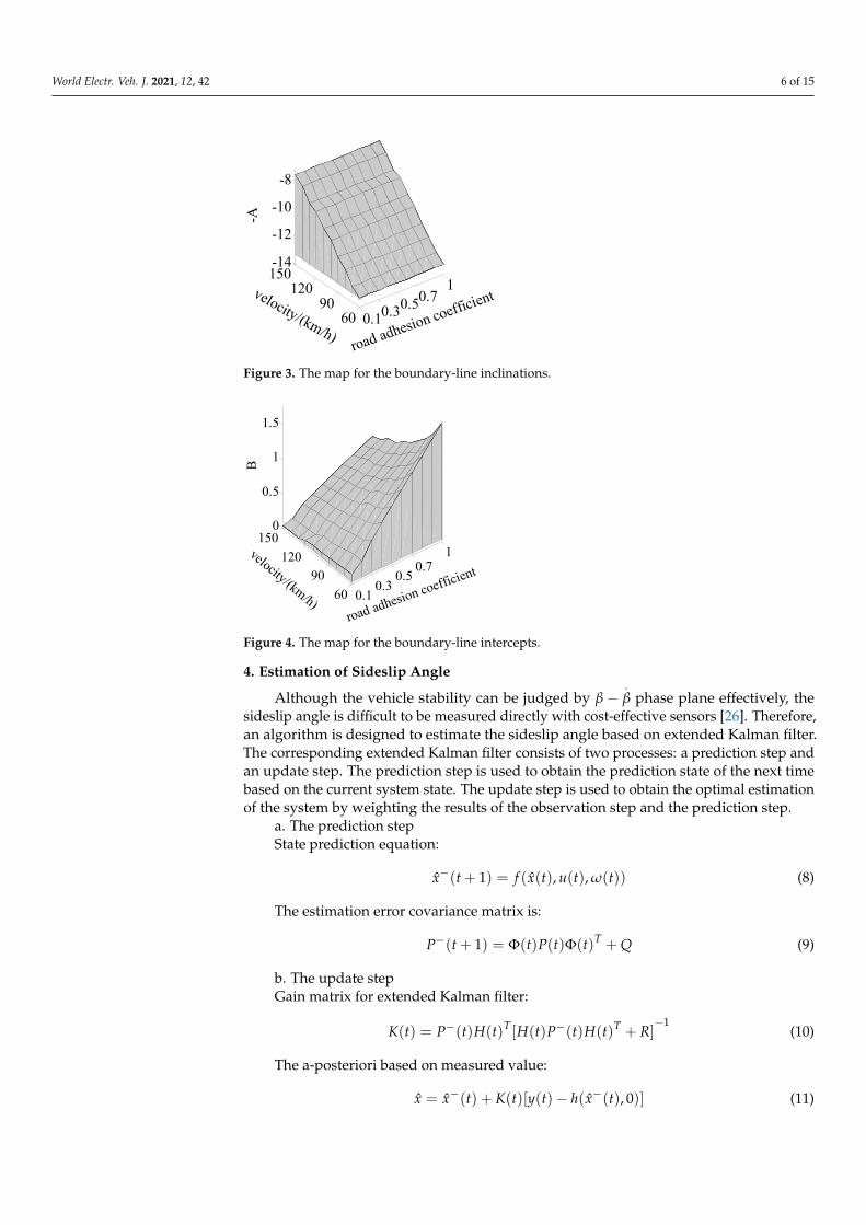
Based on the 100 groups of phase-plane diagrams drawn above, the intercepts and inclinations of 100 groups of boundary lines are obtained, and maps of the inclinations and intercepts are shown in Figures 3 and 4. On the premise of considering the velocity and accuracy of simulation, the parameters of boundary lines can be determined by a two-dimensional look-up table according to the above maps and driving conditions, so as to reasonably judge the vehicle stability, based on 𝛽 − 𝛽 phase planes.

-0.3 -0.2 0.1 0 0.1 0.2 0.3-1

-0.5

0

0.5

sideslip angle/rad

sides

lip a

ngle

/(ra

d/s)

-A=9.1B/A=0.08

-B/A=-0.08

-0.3 -0.2 -0.1 0 0.1 0.2 0.3-1

-0.5

0

0.5

1

sideslip angle/rad

sides

lip a

ngle

rate

/(rad

/s)

-A=12-B/A=-0.088

B/A=0.088

-0.3 -0.2 -0.1 0 0.1 0.2 0.3-1

-0.5

0

0.5

1

sideslip angle/rad

sides

lip a

ngle

rate

/(rad

/s)

-B/A=-0.057 -A=-12

B/A=0.057

Figure 2. Phase plane in different driving conditions (a) Vx = 120 km/h, µ = 0.8; (b) Vx = 80 km/h,µ = 0.8; and (c) Vx = 80 km/h, µ = 0.5.

3.3. Parameters Determination for Boundary Lines of β−.β Phase Planes

Based on the 100 groups of phase-plane diagrams drawn above, the intercepts andinclinations of 100 groups of boundary lines are obtained, and maps of the inclinationsand intercepts are shown in Figures 3 and 4. On the premise of considering the velocityand accuracy of simulation, the parameters of boundary lines can be determined by atwo-dimensional look-up table according to the above maps and driving conditions, so asto reasonably judge the vehicle stability, based on β−

.β phase planes.

World Electr. Veh. J. 2021, 12, 42 6 of 15World Electr. Veh. J. 2021, 12, x FOR PEER REVIEW 6 of 16

Figure 3. The map for the boundary-line inclinations.

Figure 4. The map for the boundary-line intercepts.

4. Estimation of Sideslip Angle Although the vehicle stability can be judged by 𝛽 − 𝛽 phase plane effectively, the

sideslip angle is difficult to be measured directly with cost-effective sensors [26]. There-fore, an algorithm is designed to estimate the sideslip angle based on extended Kalman filter. The corresponding extended Kalman filter consists of two processes: a prediction step and an update step. The prediction step is used to obtain the prediction state of the next time based on the current system state. The update step is used to obtain the optimal estimation of the system by weighting the results of the observation step and the predic-tion step.

a. The prediction step State prediction equation:

))(),(),(ˆ()1(ˆ ttutxftx ω=+− (8)

The estimation error covariance matrix is:

( 1) ( ) ( ) ( )TP t t P t t Q− + = Φ Φ + (9)

b. The update step Gain matrix for extended Kalman filter:

1( ) ( ) ( ) [ ( ) ( ) ( ) ]T TK t P t H t H t P t H t R− − −= + (10)

The a-posteriori based on measured value:

)]0),(ˆ()()[()(ˆˆ txhtytKtxx −− −+= (11)

Prediction matrix for the error covariance:

0.10.30.50.71

6090

120150-14

-12

-10

-8

road adhesion coefficientvelocity/(km/h)

-A

0.10.3

0.50.7

1

6090

120150

0

0.5

1

1.5

road adhesion coefficientvelocity/(km/h)

B

Figure 3. The map for the boundary-line inclinations.

World Electr. Veh. J. 2021, 12, x FOR PEER REVIEW 6 of 16

Figure 3. The map for the boundary-line inclinations.

Figure 4. The map for the boundary-line intercepts.

4. Estimation of Sideslip Angle Although the vehicle stability can be judged by 𝛽 − 𝛽 phase plane effectively, the

sideslip angle is difficult to be measured directly with cost-effective sensors [26]. There-fore, an algorithm is designed to estimate the sideslip angle based on extended Kalman filter. The corresponding extended Kalman filter consists of two processes: a prediction step and an update step. The prediction step is used to obtain the prediction state of the next time based on the current system state. The update step is used to obtain the optimal estimation of the system by weighting the results of the observation step and the predic-tion step.

a. The prediction step State prediction equation:

))(),(),(ˆ()1(ˆ ttutxftx ω=+− (8)

The estimation error covariance matrix is:

( 1) ( ) ( ) ( )TP t t P t t Q− + = Φ Φ + (9)

b. The update step Gain matrix for extended Kalman filter:

1( ) ( ) ( ) [ ( ) ( ) ( ) ]T TK t P t H t H t P t H t R− − −= + (10)

The a-posteriori based on measured value:

)]0),(ˆ()()[()(ˆˆ txhtytKtxx −− −+= (11)

Prediction matrix for the error covariance:

0.10.30.50.71

6090

120150-14

-12

-10

-8

road adhesion coefficientvelocity/(km/h)

-A

0.10.3

0.50.7

1

6090

120150

0

0.5

1

1.5

road adhesion coefficientvelocity/(km/h)

B

Figure 4. The map for the boundary-line intercepts.

4. Estimation of Sideslip Angle

Although the vehicle stability can be judged by β −.β phase plane effectively, the

sideslip angle is difficult to be measured directly with cost-effective sensors [26]. Therefore,an algorithm is designed to estimate the sideslip angle based on extended Kalman filter.The corresponding extended Kalman filter consists of two processes: a prediction step andan update step. The prediction step is used to obtain the prediction state of the next timebased on the current system state. The update step is used to obtain the optimal estimationof the system by weighting the results of the observation step and the prediction step.

a. The prediction stepState prediction equation:

x̂−(t + 1) = f (x̂(t), u(t), ω(t)) (8)

The estimation error covariance matrix is:

P−(t + 1) = Φ(t)P(t)Φ(t)T + Q (9)

b. The update stepGain matrix for extended Kalman filter:

K(t) = P−(t)H(t)T [H(t)P−(t)H(t)T + R]−1

(10)

The a-posteriori based on measured value:

x̂ = x̂−(t) + K(t)[y(t)− h(x̂−(t), 0)] (11)

World Electr. Veh. J. 2021, 12, 42 7 of 15

Prediction matrix for the error covariance:

P(t) = (I − K(t)H(t))P−(t) (12)

State equation and observation equation for the nonlinear system are as follows:{ .x(t) = f (x(t), u(t), ω(t))

y(t) = h(x(t), v(t))(13)

In Equations (8)–(13), x(t) is the state variable, u(t) is the input vector, y(t) is the outputvector, ω(t) is the process noise, v(t) is the measurement noise, Φ(t) is the state transitionmatrix, H(t) is the Jacobian matrix of the partial derivatives of function h(x(t),v(t)) to statex(t), Q is the process noise covariance matrix, R measurement noise covariance, and I is theidentity matrix.

For the research object, the following state equation is obtained based on 3 DOFvehicle model [27]:

.γ =

(l2f k f +l2

r kr)γ

IzVx+

(l f k f−lrkr)β

Iz− l f k f δ f

Iz.β = (

l f k f−lrkr

mV2x− 1)γ +

(k f +kr)β

mVx− k f δ f

mVx.Vx = βγVx + ax

(14)

The system measurement equation is as follows:

ay =(l f k f − lrkr)γ

mVx+

(k f + kr)β

m−

k f δ f

m(15)

After linearizing the model, we can get:

F(t) =

(l2

f k f +l2r kr)γ

IzVx

(l f k f−lrkr)

Iz−

(l2f k f +l2

r kr)γ

IzV2x

(l f k f−lrkr)

mV2x− 1)

(k f +kr)

mVx− 2(l f k f−lrkr)γ

mV3x

− (k f +kr)β

mV2x

+k f δ fmVx

βVx γVx βγ

(16)

H =[

(l f k f−lrkr)

mVx

(k f +kr)

m(lrkr−l f k f )

mV2x

]T(17)

Φ(t) = eF(t)∗∆t ≈ I + F(t) ∗ ∆t (18)

In the Equations (14)–(18), ay is the lateral acceleration, kf is the cornering stiffness offront axle, kr is the cornering stiffness of rear axle, F(t) is the Jacobian matrix of the partialderivatives of function f (x(t),u(t),w(t)) to state x(t), and ∆t is the sampling time. The otherletters are shown above.

When P-(t) is given an initial value of I3×3, and x̂−(t) is given an initial value of[0,0,0]T, the estimation of sideslip angle can be obtained by forming a circulative processcontinuously of the prediction step and the update step of the extended Kalman filter.

5. Design of Stability Control System for Electric Vehicle with Four IWMs5.1. Calculation of Yaw Moment

Control parameters and external disturbance have great influence on the stabilitycontrol system for electric vehicles with four IWMs [15]. In order to solve this problem,this paper selects sliding-mode control algorithm with strong robustness to determinethe required yaw moment of the vehicle. Based on the influence analysis of the drivingconditions on β −

.β phase plane, it is known that the sideslip angle under medium or

low µ road surfaces has a great impact on vehicle stability control, and the smaller thesideslip angle is, the better the vehicle handling stability is. Therefore, the sideslip angle isselected as the control variable under middle or low µ road surfaces. When the sideslip

World Electr. Veh. J. 2021, 12, 42 8 of 15

angle is introduced into the calculation of compensating yaw moment, the equation of2-DOF vehicle is:

.β =

(k f +kr)β

mVx+ (

l f k f−lrkrmVx

− 1)γ− k f δ fmVx

.γ =

(k f−kr)β

Iz+

(l f2k f +lr2kr)γ

IzVx− l f k f δ f

Iz+

∆Mβ

Iz

(19)

where ∆Mβ is the yaw moment based on β−.β phase plane. The other letters are shown above.

The design of sliding-mode controller includes the definition of sliding surface andselection of approaching rate. In order to reduce the chattering of control system, saturationfunction should be designed to replace the original sign function sgn(sβ).

The sliding surface of the sideslip angle is defined as follows:

sβ =.β−

.βd (20)

where.βd is the derivation of the ideal sideslip angle. In this paper, exponential approaching

rate is chosen to make the system reach a sliding surface quickly. The expression isas follows:

.sβ = εsgn(sβ)− ksβ (21)

where ε and k are the parameters of exponential approaching rate.The yaw moment can be obtained by deriving the above sliding surface, combining

the exponential approaching rate and the 2-DOF vehicle equation with the yaw moment.

∆Mβ = −IZ{(k f +kr)

mVx[(k f +kr)β

mVx+

(l f k f−lrkr)

mVx− 1)[

(l f k f−lrkr)β

IZ+

(l2f k f +l2

rkr)γ

IZVx− l f k f δ f

IZ]

− k f.δ f

mVx−

.βd + εβsgn(Sβ) + kβsβ}(

(l f k f−lrkr)

mVx− 1)

−1 (22)

where.δ f is the derivative of front-wheel angle and kβ is the parameter of exponential

approaching rate based on β−.β decision. The letters are shown above.

In order to eliminate chattering causes by sliding-mode control near the sliding surface,the boundary layer φ = 0.01 is introduced near sliding surface. That is the sign functionsgn(sβ) which is replaced by the saturation function sat(sβ/φ). The saturation function isas follows:

sat(sβ

φ) =

{sgn(sβ),

∣∣sβ

∣∣ > φsβ

φ ,∣∣sβ

∣∣ ≤ φ(23)

The letters are shown above.

5.2. Distribution of Wheel Longitudinal Forces

For realizing the control of vehicle stability, the yaw moment of the vehicle should beconverted to the input torques of each wheel. First of all, the torques of each wheel shouldmeet the requirements of vehicle longitudinal forces and yaw moment. In addition, theconstraints for electric vehicle with four IWMs include the limit of driving/braking forcesof IWM and road adhesion coefficients.{

∑ Fx = (T1 + T2 + T3 + T4)/R∆MZ = d[(T1 − T2) cos δ f + (T3 − T4)]/2/R (24)

Txi ≤ min(µRFzi, Tmax) (25)

where T1, T2, T3, and T4 represent the output torque of left-front wheel, right-front wheel,left-rear wheel and right-rear wheel, respectively; R is the wheel radius; Txi is torques ofeach in-wheel-motor; Fzi is the vertical forces of each wheel; and i = 1–4; Tmax is the peaktorque of in-wheel-motors. The other letters are shown above.

World Electr. Veh. J. 2021, 12, 42 9 of 15

In order to avoid the control failure caused by the longitudinal/lateral forces satu-ration of a tire, this paper takes the minimum sum of squares of wheel load rates as theoptimization objective to optimize the wheel torque distribution. The minimum sum ofsquares of wheel load rates is defined as follows:

ηi =

√F2

xi + F2yi

µFzi(26)

Considering that it is difficult to control the tire lateral forces accurately, the opti-mization objective can be simplified to minimize the sum of squares of wheel load ratesgenerated by the wheel longitudinal forces. The objective function is as follows:

minJ =4

∑i=1

F2xi

(µFzi)2 =

4

∑i=1

T2xi

(µRFzi)2 (27)

where Fxi is the longitudinal forces of each wheel. The other letters are shown above.Based on the above optimization objective function, equality constraints and inequality

constraints, a quadratic programming mathematical model is established.

minJ =12

xT Hx + CTxC (28)

where x= [Fx1 Fx2 Fx3 Fx4]T,C is a null matrix, and the expression of H is as follows:

H =

1

(µFZ1)2 0 0 0

0 1(µFZ2)

2 0 0

0 0 1(µFZ3)

2 0

0 0 0 1(µFZ4)

2

(29)

For the quadratic programming problem with equality or inequality constraints, theoptimum can be obtained by using the active set methods.

6. Cosimulation Model Based on Matlab/Simulink and Carsim

In order to assess phase planes, sideslip-angle estimation algorithm, optimal algorithmof torque distribution, and torque control method proposed in the paper, a simulationmodel for the stability control system of electric vehicles with four IWMs is built based onMatlab/Simulink and Carsim. The architecture for cosimulation model is presented in theFigure 5. The driver–vehicle–road model is established in Carsim. The other two modelsare established in Matlab/Simulink. The first is the criterion of vehicle stability model,including the estimation model of sideslip angle and 7-DOF vehicle model. The secondis the vehicle stability control model, including the calculation model of yaw momentbased on the sideslip angle, the wheel longitudinal forces distribution model, and theIWM model.

6.1. Vehicle Model

The advantage of using Carsim in the cosimulation model is that Carsim can providereliable driver–vehicle–road models to ensure the accuracy of simulation. However, thereis no electric vehicle with IWM model in Carsim. Therefore, in this paper, the electricvehicle model with 4 IWMs is obtains by changing the power transmission system schemeof traditional vehicle model in Carsim. The method is as follows: the power transmissionsystem of the traditional vehicle in Carsim is changed to external components; the IWMmodel is built in Matlab/Simulink; and the torque output from the in-wheel-motor modelis transmitted to the wheel module of Carsim.

World Electr. Veh. J. 2021, 12, 42 10 of 15

World Electr. Veh. J. 2021, 12, x FOR PEER REVIEW 10 of 16

6. Cosimulation Model Based on Matlab/Simulink and Carsim In order to assess phase planes, sideslip-angle estimation algorithm, optimal algo-

rithm of torque distribution, and torque control method proposed in the paper, a simula-tion model for the stability control system of electric vehicles with four IWMs is built based on Matlab/Simulink and Carsim. The architecture for cosimulation model is pre-sented in the Figure 5. The driver–vehicle–road model is established in Carsim. The other two models are established in Matlab/Simulink. The first is the criterion of vehicle stability model, including the estimation model of sideslip angle and 7-DOF vehicle model. The second is the vehicle stability control model, including the calculation model of yaw mo-ment based on the sideslip angle, the wheel longitudinal forces distribution model, and the IWM model.

Figure 5. Architecture diagram for cosimulation platform.

6.1. Vehicle Model The advantage of using Carsim in the cosimulation model is that Carsim can provide

reliable driver–vehicle–road models to ensure the accuracy of simulation. However, there is no electric vehicle with IWM model in Carsim. Therefore, in this paper, the electric ve-hicle model with 4 IWMs is obtains by changing the power transmission system scheme of traditional vehicle model in Carsim. The method is as follows: the power transmission system of the traditional vehicle in Carsim is changed to external components; the IWM model is built in Matlab/Simulink; and the torque output from the in-wheel-motor model is transmitted to the wheel module of Carsim.

6.2. IWM Model Based on the research objectives, the first order time-delayed system for is selected

IWM model [13]:

max

1( )min( , ) 1

TG sT T sξ∗ =

⋅ + (30)

where T is the actual torque of motor, T* is the target torque of motor, ξ is a constant determined by the motor parameters, and s is the Laplace operator. Tmax is the maximum torque at the current speed. When the motor speed is lower than the base speed, Tmax is a constant. When the motor speed is higher than the base speed, Tmax is a function of the motor speed.

Figure 5. Architecture diagram for cosimulation platform.

6.2. IWM Model

Based on the research objectives, the first order time-delayed system for is selectedIWM model [13]:

G(s)T

min(T∗, Tmax)=

1ξ · s + 1

(30)

where T is the actual torque of motor,T* is the target torque of motor, ξ is a constantdetermined by the motor parameters, and s is the Laplace operator. Tmaxis the maximumtorque at the current speed. When the motor speed is lower than the base speed, Tmax is aconstant. When the motor speed is higher than the base speed, Tmax is a function of themotor speed.

7. Simulation Evaluation7.1. Evaluation of Sideslip-Angle Estimation

The accuracy of sideslip-angle estimation is the premise of the stability control systemfor an electric vehicle with four IWMs. Therefore, we assessed the accuracy of sideslip-angle estimation through several working conditions this paper, such as double-lanechange maneuver, square-wave incremental steering, sinusoidal delay steering, etc. In thispaper, the effect of sideslip-angle estimation is illustrated by taking double-lane changemaneuvers under two velocities as examples. The road adhesion coefficient is 0.8, and thevehicle velocity is 40 km/h and 100 km/h, respectively. The simulation results are shownin Figures 6 and 7.

World Electr. Veh. J. 2021, 12, x FOR PEER REVIEW 11 of 16

7. Simulation Evaluation 7.1. Evaluation of Sideslip-Angle Estimation

The accuracy of sideslip-angle estimation is the premise of the stability control sys-tem for an electric vehicle with four IWMs. Therefore, we assessed the accuracy of side-slip-angle estimation through several working conditions this paper, such as double-lane change maneuver, square-wave incremental steering, sinusoidal delay steering, etc. In this paper, the effect of sideslip-angle estimation is illustrated by taking double-lane change maneuvers under two velocities as examples. The road adhesion coefficient is 0.8, and the vehicle velocity is 40 km/h and 100 km/h, respectively. The simulation results are shown in Figures 6 and 7.

(a) (b)

Figure 6. Estimation for sideslip angle (when Vx is 40 km/h and μ is 0.8) (a) Lateral acceleration. (b) Sideslip angle.

It can be seen from Figure 6 that when the vehicle velocity is 40 km/h, the lateral acceleration of vehicle is less than 0.4 g, and the vehicle is in a stable state. The estimation of sideslip angle by the extended Kalman filter algorithm can well follow the output value of Carsim.

(a) (b)

Figure 7. Estimation for sideslip angle (when Vx is 100 km/h and μ is 0.8) (a) Lateral acceleration. (b) Sideslip angle.

It can be known from Figure 7 that the lateral acceleration of the vehicle is more than 0.4 g when the vehicle velocity is 100 km/h, indicating that the vehicle is in an unstable state. The estimation of sideslip angle by the extended Kalman filter algorithm is slightly less than the output value of Carsim at the peak value, and other parts can follow the output value of Carsim well.

The simulation results show that the proposed estimation algorithm for sideslip an-gle can follow the output value of Carsim, no matter if the vehicle is stable or unstable, and can meet the requirements of stability control system of electric vehicle with four IWMs.

0 2 4 6 8 10 12 14 16-0.4

-0.3

-0.2

-0.1

0

0.1

0.2

0.3

time/s

late

ral a

ccel

erat

ion/

g

0 2 4 6 8 10 12 14 16-0.015

-0.01

-0.005

0

0.005

0.01

0.015

time/s

side

slip

angl

e/ra

d

estimated valuevalue from Carsim

0 2 4 6 8 10-0.8

-0.6

-0.4

-0.2

0

0.2

0.4

0.6

0.8

time /s

late

ral a

ccel

erat

ion/

g

0 2 4 6 8 10-0.05-0.04-0.03-0.02-0.01

00.010.020.030.040.05

time/s

side

slip

angl

e/ra

d

estimated valuevalue from Carsim

Figure 6. Estimation for sideslip angle (when Vx is 40 km/h and µ is 0.8) (a) Lateral acceleration. (b) Sideslip angle.

World Electr. Veh. J. 2021, 12, 42 11 of 15

World Electr. Veh. J. 2021, 12, x FOR PEER REVIEW 11 of 16

7. Simulation Evaluation 7.1. Evaluation of Sideslip-Angle Estimation

The accuracy of sideslip-angle estimation is the premise of the stability control sys-tem for an electric vehicle with four IWMs. Therefore, we assessed the accuracy of side-slip-angle estimation through several working conditions this paper, such as double-lane change maneuver, square-wave incremental steering, sinusoidal delay steering, etc. In this paper, the effect of sideslip-angle estimation is illustrated by taking double-lane change maneuvers under two velocities as examples. The road adhesion coefficient is 0.8, and the vehicle velocity is 40 km/h and 100 km/h, respectively. The simulation results are shown in Figures 6 and 7.

(a) (b)

Figure 6. Estimation for sideslip angle (when Vx is 40 km/h and μ is 0.8) (a) Lateral acceleration. (b) Sideslip angle.

It can be seen from Figure 6 that when the vehicle velocity is 40 km/h, the lateral acceleration of vehicle is less than 0.4 g, and the vehicle is in a stable state. The estimation of sideslip angle by the extended Kalman filter algorithm can well follow the output value of Carsim.

(a) (b)

Figure 7. Estimation for sideslip angle (when Vx is 100 km/h and μ is 0.8) (a) Lateral acceleration. (b) Sideslip angle.

It can be known from Figure 7 that the lateral acceleration of the vehicle is more than 0.4 g when the vehicle velocity is 100 km/h, indicating that the vehicle is in an unstable state. The estimation of sideslip angle by the extended Kalman filter algorithm is slightly less than the output value of Carsim at the peak value, and other parts can follow the output value of Carsim well.

The simulation results show that the proposed estimation algorithm for sideslip an-gle can follow the output value of Carsim, no matter if the vehicle is stable or unstable, and can meet the requirements of stability control system of electric vehicle with four IWMs.

0 2 4 6 8 10 12 14 16-0.4

-0.3

-0.2

-0.1

0

0.1

0.2

0.3

time/s

late

ral a

ccel

erat

ion/

g

0 2 4 6 8 10 12 14 16-0.015

-0.01

-0.005

0

0.005

0.01

0.015

time/s

side

slip

angl

e/ra

d

estimated valuevalue from Carsim

0 2 4 6 8 10-0.8

-0.6

-0.4

-0.2

0

0.2

0.4

0.6

0.8

time /s

late

ral a

ccel

erat

ion/

g

0 2 4 6 8 10-0.05-0.04-0.03-0.02-0.01

00.010.020.030.040.05

time/s

side

slip

angl

e/ra

d

estimated valuevalue from Carsim

Figure 7. Estimation for sideslip angle (when Vx is 100 km/h and µ is 0.8) (a) Lateral acceleration. (b) Sideslip angle.

It can be seen from Figure 6 that when the vehicle velocity is 40 km/h, the lateralacceleration of vehicle is less than 0.4 g, and the vehicle is in a stable state. The estimationof sideslip angle by the extended Kalman filter algorithm can well follow the output valueof Carsim.

It can be known from Figure 7 that the lateral acceleration of the vehicle is more than0.4 g when the vehicle velocity is 100 km/h, indicating that the vehicle is in an unstablestate. The estimation of sideslip angle by the extended Kalman filter algorithm is slightlyless than the output value of Carsim at the peak value, and other parts can follow theoutput value of Carsim well.

The simulation results show that the proposed estimation algorithm for sideslip anglecan follow the output value of Carsim, no matter if the vehicle is stable or unstable, andcan meet the requirements of stability control system of electric vehicle with four IWMs.

7.2. Evaluation of Torque Distribution

The double-lane change maneuver is used to verify the correctness of quadraticprogramming torque distribution. The road adhesion coefficient is 0.8, and the vehiclevelocity is 130 km/h. The simulation results are as follows:

As shown in Figure 8a, vehicle trajectories without stability control have a largedeviation from the target trajectories. The vehicle tends to be unstable. However, the directyaw moment control (DYC), based on the average torque distribution and the optimaltorque distribution, can make the deviation between the actual trajectories and the targettrajectories smaller. As shown in Figure 8b, the DYC, based on optimal torque distribution,can make the vehicle yaw rate closer to the target value than the average distributionmethod. As shown in Figure 8c,d, the sideslip angle, based on optimal torque distributionmethod, is limited to a small range, and the β −

.β phase portraits return to the origin

more quickly than that without control. This shows that the vehicle is more stable, andit can be known that the control effect of optimal torque distribution method is betterthan the average distribution method. As shown in Figure 8e–g, the torque value of eachwheel, based on the optimal torque distribution, is consistent with trend of the wheelvertical forces. This distribution mode enables each wheel to adjust the longitudinal forcesreasonably and avoid the vertical forces from reaching the longitudinal forces saturationrapidly, especially if the tire vertical force is small. As shown in Figure 8h, the sum ofthe wheel load rates based on the optimal torque distribution method is smaller than thatof average torque distribution method. This shows that the optimal torque distributioncontrol can make the torque distribution of each wheel more reasonable, and the adjustablemargin of longitudinal forces is larger, which can make the vehicle more stable.

World Electr. Veh. J. 2021, 12, 42 12 of 15

World Electr. Veh. J. 2021, 12, x FOR PEER REVIEW 12 of 16

7.2. Evaluation of Torque Distribution The double-lane change maneuver is used to verify the correctness of quadratic pro-

gramming torque distribution. The road adhesion coefficient is 0.8, and the vehicle veloc-ity is 130 km/h. The simulation results are as follows:

As shown in Figure 8a, vehicle trajectories without stability control have a large devia-tion from the target trajectories. The vehicle tends to be unstable. However, the direct yaw moment control (DYC), based on the average torque distribution and the optimal torque distribution, can make the deviation between the actual trajectories and the target trajecto-ries smaller. As shown in Figure 8b, the DYC, based on optimal torque distribution, can make the vehicle yaw rate closer to the target value than the average distribution method. As shown in Figure 8c,d, the sideslip angle, based on optimal torque distribution method, is limited to a small range, and the 𝛽 − 𝛽 phase portraits return to the origin more quickly than that without control. This shows that the vehicle is more stable, and it can be known that the control effect of optimal torque distribution method is better than the average distribution method. As shown in Figure 8e–g, the torque value of each wheel, based on the optimal torque distribution, is consistent with trend of the wheel vertical forces. This distribution mode enables each wheel to adjust the longitudinal forces reasonably and avoid the vertical forces from reaching the longitudinal forces saturation rapidly, espe-cially if the tire vertical force is small. As shown in Figure 8h, the sum of the wheel load rates based on the optimal torque distribution method is smaller than that of average torque distribution method. This shows that the optimal torque distribution control can make the torque distribution of each wheel more reasonable, and the adjustable margin of longitudinal forces is larger, which can make the vehicle more stable.

(a) (b)

(c) (d)

0 70 140 210 280 0 70 140 210-1

0

1

2

3

4

longitudinal displacement/m

late

ral d

ispla

cem

ent/m

target trajectoryuncontrolledaverage distribution of torqueoptimal distribution of torque

0 2 4 6 8

-0.3

-0.2

-0.1

0

0.1

0.2

0.3

0.4

time/s

yaw

rate

/(rad

/s)

target aim valueaverage distribution of torqueoptimal distribution of torque

0 1 2 3 4 5 6 7 8-0.1

-0.05

0

0.05

0.1

time/s

sides

lip a

ngle

/rad

average distribution of torqueoptimal distribution of torque

-0.1 -0.05 0 0.05 0.1-0.4

-0.3

-0.2

-0.1

0

0.1

0.2

0.3

0.4

sideslip angle /rad

sides

lip ra

te /(

rad/

s)

uncontrolledaverage distribution of torqueoptimal distribution of torque

World Electr. Veh. J. 2021, 12, x FOR PEER REVIEW 13 of 16

(e) (f)

(g) (h)

Figure 8. Verification of optimal torque distribution (a) trajectory, (b) yaw rate, (c) sideslip angle, (d) 𝛽 − 𝛽 phase plane, (e) wheel torque when average distribution, (f) wheel torque when optimal distribution, (g) vertical load of each wheel, and (h) sum of wheel load rates.

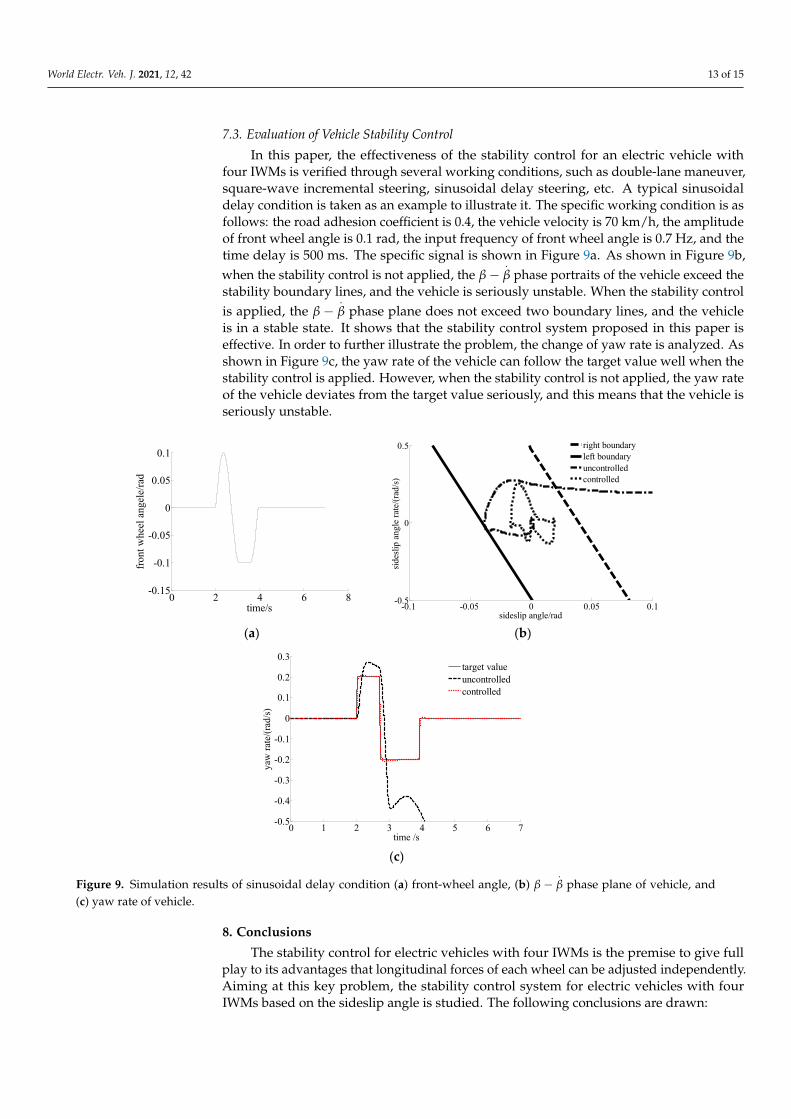
7.3. Evaluation of Vehicle Stability Control In this paper, the effectiveness of the stability control for an electric vehicle with four

IWMs is verified through several working conditions, such as double-lane maneuver, square-wave incremental steering, sinusoidal delay steering, etc. A typical sinusoidal de-lay condition is taken as an example to illustrate it. The specific working condition is as follows: the road adhesion coefficient is 0.4, the vehicle velocity is 70 km/h, the amplitude of front wheel angle is 0.1 rad, the input frequency of front wheel angle is 0.7 Hz, and the time delay is 500 ms. The specific signal is shown in Figure 9a. As shown in Figure 9b, when the stability control is not applied, the 𝛽 − 𝛽 phase portraits of the vehicle exceed the stability boundary lines, and the vehicle is seriously unstable. When the stability con-trol is applied, the β-β phase plane does not exceed two boundary lines, and the vehicle is in a stable state. It shows that the stability control system proposed in this paper is ef-fective. In order to further illustrate the problem, the change of yaw rate is analyzed. As shown in Figure 9c, the yaw rate of the vehicle can follow the target value well when the stability control is applied. However, when the stability control is not applied, the yaw rate of the vehicle deviates from the target value seriously, and this means that the vehicle is seriously unstable.

0 1 2 3 4 5 6 7 8-300

-200

-100

0

100

200

300

time/s

whe

el to

rque

/Nm

torque of left front wheel torque of right front wheel torque of left rear wheel torque of right rear wheel

0 1 2 3 4 5 6 7 8-300

-200

-100

0

100

200

300

time/s

whe

el to

rque

/Nm

torque of left front wheeltorque of right front wheeltorque of left rear wheeltorque of right rear wheel

0 1 2 3 4 5 6 7 81500

2000

2500

3000

3500

4000

4500

time/s

verti

cal f

orce

/N

force of left front wheel force of right front wheelforce of left rear wheelforce of right rear wheel

0 1 2 3 4 5 6 7 80

0.5

1

1.5

2

2.5

3

time/s

sum

of w

heel

load

rate

s

average distribution of torqueoptimal distribution of torque

Figure 8. Verification of optimal torque distribution (a) trajectory, (b) yaw rate, (c) sideslip angle, (d) β−.β phase plane,

(e) wheel torque when average distribution, (f) wheel torque when optimal distribution, (g) vertical load of each wheel, and(h) sum of wheel load rates.

World Electr. Veh. J. 2021, 12, 42 13 of 15

7.3. Evaluation of Vehicle Stability Control

In this paper, the effectiveness of the stability control for an electric vehicle withfour IWMs is verified through several working conditions, such as double-lane maneuver,square-wave incremental steering, sinusoidal delay steering, etc. A typical sinusoidaldelay condition is taken as an example to illustrate it. The specific working condition is asfollows: the road adhesion coefficient is 0.4, the vehicle velocity is 70 km/h, the amplitudeof front wheel angle is 0.1 rad, the input frequency of front wheel angle is 0.7 Hz, and thetime delay is 500 ms. The specific signal is shown in Figure 9a. As shown in Figure 9b,when the stability control is not applied, the β−

.β phase portraits of the vehicle exceed the

stability boundary lines, and the vehicle is seriously unstable. When the stability controlis applied, the β−

.β phase plane does not exceed two boundary lines, and the vehicle

is in a stable state. It shows that the stability control system proposed in this paper iseffective. In order to further illustrate the problem, the change of yaw rate is analyzed. Asshown in Figure 9c, the yaw rate of the vehicle can follow the target value well when thestability control is applied. However, when the stability control is not applied, the yaw rateof the vehicle deviates from the target value seriously, and this means that the vehicle isseriously unstable.

World Electr. Veh. J. 2021, 12, x FOR PEER REVIEW 14 of 16

(a) (b)

(c)

Figure 9. Simulation results of sinusoidal delay condition (a) front-wheel angle, (b) 𝛽 − 𝛽 phase plane of vehicle, and (c) yaw rate of vehicle.

8. Conclusions The stability control for electric vehicles with four IWMs is the premise to give full

play to its advantages that longitudinal forces of each wheel can be adjusted inde-pendently. Aiming at this key problem, the stability control system for electric vehicles with four IWMs based on the sideslip angle is studied. The following conclusions are drawn:

(1) Considering the key factors such as vehicle velocities and road adhesion coeffi-cients, the criterion of vehicle stability based on 𝛽 − 𝛽 phase planes is established, and 𝛽 − 𝛽 phase planes are got by a 7-DOF vehicle model. On the premise of considering the velocities and accuracy of simulation, maps of inclinations and intercepts for boundary lines of 𝛽 − 𝛽 phase planes are established based on a large number of simulations, and it is used in the stability control system for electric vehicles with four IWMs through look-ing up a two-dimensional table.

(2) To solve the problem that sideslip angle is difficult to measure directly, an esti-mation algorithm for sideslip angle based on the extended Kalman filter is designed. Based on sliding-mode control, the DYC is proposed, together with wheel driving/braking torque distribution control method which takes the minimum sum of squares of wheel load rates as the optimization objective.

(3) Based on MATLAB/Simulink and Carsim, a cosimulation model for stability con-trol of electric vehicles with four IWMs is built. The accuracy of 𝛽 − 𝛽 phase plane, esti-mation algorithm for sideslip angle, optimal algorithm of torque distribution, and torque control method are assessed. Relevant research can provide some references for the de-velopment of stability control system of electric vehicles with four IWMs.

0 2 4 6 8-0.15

-0.1

-0.05

0

0.05

0.1

time/s

front

whe

el a

ngel

e/ra

d

-0.1 -0.05 0 0.05 0.1-0.5

0

0.5

sideslip angle/rad

sides

lip a

ngle

rate

/(rad

/s)

right boundaryleft boundaryuncontrolledcontrolled

0 1 2 3 4 5 6 7-0.5

-0.4

-0.3

-0.2

-0.1

0

0.1

0.2

0.3

time /s

yaw

rate

/(rad

/s)

target valueuncontrolledcontrolled

Figure 9. Simulation results of sinusoidal delay condition (a) front-wheel angle, (b) β−.β phase plane of vehicle, and

(c) yaw rate of vehicle.

8. Conclusions

The stability control for electric vehicles with four IWMs is the premise to give fullplay to its advantages that longitudinal forces of each wheel can be adjusted independently.Aiming at this key problem, the stability control system for electric vehicles with fourIWMs based on the sideslip angle is studied. The following conclusions are drawn:

World Electr. Veh. J. 2021, 12, 42 14 of 15

(1) Considering the key factors such as vehicle velocities and road adhesion coefficients,the criterion of vehicle stability based on β−

.β phase planes is established, and β−

.β phase

planes are got by a 7-DOF vehicle model. On the premise of considering the velocities andaccuracy of simulation, maps of inclinations and intercepts for boundary lines of β−

.β

phase planes are established based on a large number of simulations, and it is used inthe stability control system for electric vehicles with four IWMs through looking up atwo-dimensional table.

(2) To solve the problem that sideslip angle is difficult to measure directly, an estima-tion algorithm for sideslip angle based on the extended Kalman filter is designed. Based onsliding-mode control, the DYC is proposed, together with wheel driving/braking torquedistribution control method which takes the minimum sum of squares of wheel load ratesas the optimization objective.

(3) Based on MATLAB/Simulink and Carsim, a cosimulation model for stabilitycontrol of electric vehicles with four IWMs is built. The accuracy of β−

.β phase plane,

estimation algorithm for sideslip angle, optimal algorithm of torque distribution, andtorque control method are assessed. Relevant research can provide some references for thedevelopment of stability control system of electric vehicles with four IWMs.

Author Contributions: Conceptualization, K.Y.; Formal analysis, D.D. and Z.T.; Funding acquisition,K.Y.; Methodology, K.Y. and D.D.; Project administration, K.Y.; Software, C.M. and Z.T.; Validation,K.Y. and Y.C.; Writing—original draft, Y.C. and G.W.; Writing—review and editing, K.Y. and D.D. Allauthors have read and agreed to the published version of the manuscript.

Funding: This research was funded by National Natural Science Foundation of China (Grant No.51605265) and Key research and development program of Shandong province of China (Grant No.2018GGX105010).

Conflicts of Interest: The authors declare no conflict of interest.

References1. Asiabar, A.; Kazemi, R. A direct yaw moment controller for a four in-wheel motor drive electric vehicle using adaptive sliding

mode control. Proc. Inst. Mech. Eng. Part K J. Multi Body Dyn. 2019, 233, 549–567. [CrossRef]2. Han, Z.; Xu, N.; Chen, H. Energy-efficient control of electric vehicles based on linear quadratic regulator and phase plane analysis.

Appl. Energy 2018, 213, 639–657. [CrossRef]3. Rauh, J.; Ammon, D. System dynamics of electrified vehicles: Some facts, thoughts, and challenges. Veh. Syst. Dyn. 2011, 49,

1005–1020.4. Vignati, M.; Sabbioni, E.; Tarsitano, D. Torque vectoring control for IWM vehicles. Int. J. Veh. Perform. 2016, 3, 202–324.5. Li, M.X.; Jia, Y.M.; Matsuno, F. Attenuating diagonal decoupling with robustness for velocity-varying 4WS vehicles. Control Eng.

Pract. 2016, 56, 49–59. [CrossRef]6. Jin, H.; Li, S.J. Research on vehicle stability control based on limit velocity. Automot. Eng. 2018, 40, 48–56.7. Zhang, R.Y.; Huang, H.; Zhao, L.F.; Yang, J. Coordinated control of EPS and ESP based on function allocation and multi-objective

fuzzy decision. J. Mech. Eng. 2014, 50, 99–106. [CrossRef]8. Jian, L. Research Status and Development Prospect of Electric Vehicles Based on Hub Motor. In Proceedings of the China

International Conference on Electricity Distribution (CICED), Tianjin, China, 17–19 September 2018; pp. 126–129.9. Lin, C.; Cheng, X.Q. A Traction Control Strategy with an Efficiency Model in a Distributed Driving Electric Vehicle. Sci. World J.

2014, 2014, 261085. [CrossRef] [PubMed]10. Kim, D.; Hwang, S.; Kim, H. Vehicle Stability Enhancement of Four-Wheel-Drive Hybrid Electric Vehicle Using Rear Motor

Control. IEEE Trans. Veh. Technol. 2008, 57, 727–735.11. Mousavinejad, E.; Han, Q.L.; Yang, F.W.; Zhu, Y.; Vlacic, L. Integrated control of road vehicles dynamics via advanced terminal

sliding mode control. Veh. Syst. Dyn. 2017, 55, 268–294. [CrossRef]12. Song, Y.; Chen, W.W.; Chen, L.Q. Research on integrated control of vehicle stability system and four-wheel steering system. China

Mech. Eng. 2014, 25, 2788–2794.13. Wu, D.M. Research on Dynamic Control Mechanism and Control Strategy of Distributed Drive Electric Vehicle. Ph.D. Thesis, Jilin

University, Changchun, China, 2015.14. Kim, H.; Park, J.; Jeon, K. Integrated control strategy for torque vectoring and electronic stability control for in wheel motor EV. In

Proceedings of the 2013 World Electric Vehicle Symposium and Exhibition (EVS27), Barcelona, Spain, 17–20 November 2013;pp. 1–7.

World Electr. Veh. J. 2021, 12, 42 15 of 15

15. Gutierrez, J.; Romo, J.J.; Gonz’lez, M.I.; Canibano, E.; Merino, J.C. Control Algorithm Development for Independent WheelTorque Distribution with 4 In-wheel Electric Motors. In Proceedings of the 2011 UKSim 5th European Symposium on ComputerModeling and Simulation, Madrid, Spain, 16–18 November 2011; pp. 257–262.

16. Yu, Z.P.; Leng, B.; Xiong, L.; Feng, Y. Vehicle Stability Criteria Combined with Double Line Method and Yaw Velocity Method.J. Tongji Univ. Nat. Sci. Ed. 2015, 12, 1841–1849.

17. Jin, X.; Yin, G.; Chen, J.; Chen, N. Analysis of Lateral Stability Region for Lightweight Electric Vehicle Using Phase Plane Approach.In Proceedings of the 2019 Chinese Control. And Decision Conference (CCDC), Nanchang, China, 3–5 June 2019; pp. 5461–5466.

18. Ksjonov, A.; Ricciardi, V.; Vodovozov, V.; Augsburg, K. Trajectory Phase-Plane Method—Based Analysis of Stability andPerformance of a Fuzzy Logic Controller for an Anti-Lock Braking System. In Proceedings of the 2019 IEEE InternationalConference on Mechatronics (ICM), Ilmenau, Germany, 18–20 March 2019; pp. 602–607.

19. Shen, H.; Tan, Y.S. Vehicle handling and stability control by the cooperative control of 4WS and DYC. Mod. Phys. Lett. B 2017, 31,19–21. [CrossRef]

20. Sitthiracha, S.; Koetniyom, S.; Phanomchoeng, G. Combination of Active Braking and Torque Vectoring in Electronic StabilityControl for Four-Wheel Independent Drive Electric Vehicle. In Proceedings of the 2019 Research, Invention, and InnovationCongress (RI2C), Bangkok, Thailand, 11–13 December 2019; pp. 1–5.

21. Zhai, L.; Sun, T.; Wang, J. Electronic Stability Control Based on Motor Driving and Braking Torque Distribution for a FourIn-Wheel Motor Drive Electric Vehicle. IEEE Trans. Veh. Technol. 2016, 65, 4726–4739. [CrossRef]

22. Li, J.W.; Cui, X.L. Steering stability improvement of electric vehicle by DYC based on new target defination. In Proceedings of the2009 IEEE International Conference on Intelligent Computing and Intelligent Systems, Shanghai, China, 20–22 November 2009;pp. 457–461.

23. Chung, T.; Yi, K. Design and Evaluation of Sideslip Angle-Based Vehicle Stability Control Scheme on a Virtual Test Track. IEEETrans. Control. Syst. Technol. 2006, 14, 224–234. [CrossRef]

24. Zhang, C.C.; Xiao, Q.S.; He, L. The influence of centroid side Angle on vehicle stability. Automot. Eng. 2011, 33, 277–282.25. Guo, Y.S.; Lu, Y.P.; Fu, R.; Yang, F. Simulation Analysis of Transverse Stability of Large Bus. China J. Highw. Transp. 2018, 31,

156–164.26. Xie, X.Y. Research on Integrated Control Method of Control Stability of Distributed Electric Vehicle. Ph.D. Thesis, Jilin University,

Changchun, China, 2018.27. Lin, C.; Peng, C.L.; Cao, W.K. Sliding Mode Variable Structure Control for Stability of Independently Driven Electric Vehicle.

Automot. Eng. 2015, 37, 132–138.