Stability and conditioning in numerical analysis

European Society of Computational Methodsin Sciences and Engineering (ESCMSE)

Journal of Numerical Analysis,Industrial and Applied Mathematics

(JNAIAM)vol. 1, no. 1, 2006, pp. 91-112

ISSN 1790–8140

Stability and Conditioning in Numerical Analysis

Felice Iavernaro∗, Francesca Mazzia∗ and Donato Trigiante†

∗ Dipartimento di Matematica, Universita di Bari, Via Orabona 4, I-70125 Bari (Italy),[email protected], [email protected], fax:+39 080 5460612.

† Dip. di Energetica, Universita di Firenze, via C. Lombroso 6/17, I-50134 Firenze (Italy),[email protected].

Received 1 February, 2006; accepted in revised form 13 March, 2006

Abstract: The terms stability and conditioning are used with a variety of meanings inNumerical Analysis. All of them have in common the general concept of the response of acomputational algorithm to perturbations arising either from the data or from the specificarithmetic used on computers. In this paper we shall review the two concepts by usingsimple examples taken from both linear algebra and numerical methods for ODEs.

c© 2006 European Society of Computational Methods in Sciences and Engineering

Keywords: Conditioning, stability, stiffness, dynamical systems, boundary value problems,ordinary differential equations, numerical linear algebra

Mathematics Subject Classification: 65F35, 65L20.

1 Introduction

Even though I have not always been able to makedifficult things easy, never have I made easy thingsdifficult.

F. G. Tricomi

The notion of stability in mathematics derives from the analogous notion in mechanics. In itssimplest form, it regards the behavior of the motion of a system when the state vector is moved awayfrom its equilibrium. Three ingredients enter the definition: the existence of a reference solution,i.e. the equilibrium (usually a point or a periodic orbit in the phase space), the perturbation ofthe initial status (e.g. the initial conditions) and the duration of the motion, which is supposedto be infinite. The definition was then extended to more general systems and to different kinds ofperturbations, and now it is one of the most important concepts in the qualitative theory of bothdifferential and difference equations.

One of the important things to be analysed concerned the different behavior of the solutionaround the equilibrium. To allow this to be done, it was necessary to add, to the older concepts

92 Felice Iavernaro, Francesca Mazzia and Donato Trigiante

(i.e. stability, asymptotic stability and instability), new ones such as contractivity, uniform sta-bility, orbital stability etc. Starting from the pioneering work of Poincare, the qualitative studyof dynamical systems became so wide as to encompass different branches of investigation suchas bifurcation theory, generalizations of dynamics to topological and probability spaces, ergodictheory, holomorphic dynamics, shadowing theory.

Not all of them are considered in Numerical Analysis (NA in the following), for reasons thatwill be clear in the following sections. On the contrary, however, there are specific facets that areconsidered more important in NA than elsewhere.

More general perturbations than those introduced in the initial conditions are likewise consid-ered in the qualitative theory of dynamical systems. An example of this is the important conceptof stability under perturbation of the whole system (usually called total stability). This kind ofperturbation is often considered in NA where the source of errors, due to the finite precisionarithmetic, can be viewed as a perturbation of the entire set of computations. In other words, anumerical algorithm is not only perturbed by the errors in the data (perturbation with respect tothe initial data), but also by the errors arising in the process of computation.

Many problems either do not last for a long (in principle, infinite) time, and/or do not havean equilibrium at all. For example, a boundary value problem has a solution on a finite interval oftime and for this problem the above concept of stability no longer applies as it stands. Analystsused to distinguish such problems as being well posed or ill-posed, depending on whether thesolution depends continuously on the boundary conditions or not. This is not enough for the NApurpose, where a more refined distinction is needed. Numerical Analysts would like to know if suchdependence, although continuous, could be disastrous for the error growth. This need has requiredthe introduction of the concept of conditioning of a problem. The notion of conditioning is, toa certain extent, more general than that of stability. On the other hand, it does not distinguishbetween the different kinds of qualitative behavior, which are useful in many questions. In thefollowing sections we shall report the respective precise definitions and we shall present a few simpleexamples showing where they are used in NA.

Often, in the literature, two or more concepts, such as, e.g., discretization (in the case wherethe original problem is continuous), the stability of the algorithms and the ability of the arithmeticsystem implemented on the computers to perform operations with acceptable relative errors, areinterlaced. We agree almost completely with the following statements taken from Lax and Richmyer[17], (written in 1956!).

We shall not be concerned with rounding errors..., but it will be evident to the reader that thereis an intimate connection between stability and practicality of the equations from the point of viewof growth and the amplification of rounding errors... ( Some authors) define stability in terms of thegrowth of rounding errors. However we have a slight preference for the ( our) definition, (i.e. inde-pendent of the rounding errors) because it emphasizes that stability still has to be considered, evenif the rounding errors are negligible, unless, of course, the initial data are chosen with diabolic careso as to be exactly free of those components that would be unduly amplified if they were present.

Similar concepts were stated by Dahlquist at almost the same time [11, 12].

The slight modification that, fifty years later, we would introduce is only a deeper considerationof the practicality of the equations.

Seldom, will we consider the effect of the rounding errors, but for sake of clarity, it is convenientto consider the questions as being distinct as long as possible. Most of the examples presented here-after have been deliberately chosen to be as trivial as possible in order to facilitate the elucidationof the concepts introduced.


Stability and conditioning in Numerical Analysis 93

2 Conditioning and stiffness in discrete dynamics

More often than it is thought, numerical algorithms can be considered as discrete dynamical systemsaround critical points (equilibria), see e.g. [19, 23]. The spaces where such dynamics is placed mayvary considerably, ranging from R, or RN , to the space of N×N real or complex matrices. For thisreason, we shall refer to the well established concepts of stability used in the theory of dynamicalsystems (either continuous or discrete). In particular we shall consider Asymptotic Stability (AS),(marginal) stability and instability. Their precise definition can be found for example in [16].

Remark 2.1 Stability and AS refer to particular solutions (usually equilibria) and not to equa-tions (and then to methods in NA). Of course, if the equilibrium is unique, then the equation ischaracterized by the behavior of the solutions around it. The same may be true when the equilibriaare many and all of them show up the same qualitative behavior (this is the case, for example, ofNewton’s method). In such cases it is possible to use, without ambiguity, terminology such as stableequations, stable methods, stable problems, etc. We shall use such an extension of the terminology,because it is of common use in NA.

Not all problems however fit in the above framework. For example, Boundary Value Problems(BVPs) do not have equilibria at all and then the definitions of stability do not apply. For thepurposes of NA, knowing that the process of computation takes place around an asymptoticallystable equilibrium point is often not enough. Furthermore, the information that the solutionwill tend to an equilibrium or, equivalently, that the difference between the solution and theequilibrium will eventually tend to zero does not prevent the intermediate value of the solutionbecoming dangerously large. It is necessary to introduce parameters which monitor such behavior.

In the present section we will consider discrete dynamical systems coupled with either initialor boundary conditions. In order to make the introduction and interpretation of the monitoringparameters as easy as possible, we will consider the class of linear autonomous systems of the form

{zn+1 = Azn + b,B0z0 +B1zN+1 = η,

(1)

where zn, b ∈ Cs and A,B0, B1 ∈ Cs×s. In the next sections we will present more general (nonautonomous/nonlinear) systems, as well as their definitions for continuous systems, including anoutline of their use to attain a correct simulation of a continuous system by means of a numericalmethod.

The matrices B0 and B1 appearing in the additional condition will be assumed to be such thatdet(B0 +B1A

N+1) 6= 0, which guarantees the existence and uniqueness of the solution of (1). Wealso observe that the choice B0 = I (I is the identity matrix of appropriate size) and B1 = 0 makes(1) an Initial Value Problem (IVP). In such a case, if λ = 1 is not an eigenvalue of A, (1) willadmit a unique equilibrium point z = (I − A)−1b. Furthermore one can allow N to be arbitrarylarge to carry out a study of the long time behavior of the solution as required by the stabilityanalysis.

A perturbation δ introduced in the data η will produce a perturbed solution zn satisfyingzn+1 = Azn + b and B0z0 +B1zN+1 = η + δ, and therefore the error yn = zn − zn will satisfy theautonomous system

{yn+1 = Ayn,B0y0 +B1yN+1 = δ,

(2)


https://www.researchgate.net/publication/266255258_Theory_of_Difference_Equation-Numerical_Methods_and_Applications?el=1_x_8&enrichId=rgreq-d1529630-6182-4eb4-855a-302d77def991&enrichSource=Y292ZXJQYWdlOzI2NTk1NDY4MTtBUzoxNjE2NzE5MjY1MjU5NTJAMTQxNTU1Njk5OTIzNw==

https://www.researchgate.net/publication/247632689_Stability_of_Difference_Equations_and_Convergence_of_Iterative_Processes?el=1_x_8&enrichId=rgreq-d1529630-6182-4eb4-855a-302d77def991&enrichSource=Y292ZXJQYWdlOzI2NTk1NDY4MTtBUzoxNjE2NzE5MjY1MjU5NTJAMTQxNTU1Njk5OTIzNw==

https://www.researchgate.net/publication/200175477_Dynamical_Systems_and_Numerical_Analysis?el=1_x_8&enrichId=rgreq-d1529630-6182-4eb4-855a-302d77def991&enrichSource=Y292ZXJQYWdlOzI2NTk1NDY4MTtBUzoxNjE2NzE5MjY1MjU5NTJAMTQxNTU1Njk5OTIzNw==


which we assume as our test problem. In order to study the way the perturbation term δ affectsthe error yn, we introduce the following parameters:

κd(N, δ) =1

‖δ‖ maxi=0,...,N+1

‖yi‖, κd(N) = maxδκd(N, δ),

γd(N, δ) =1

N‖δ‖N∑

i=1

‖yi‖, γd(N) = maxδγd(N, δ).

(3)

Note that in the IVP case, the stability properties of linear systems being global in character,the perturbation term δ may be of any size; likewise linearity also implies that κd and γd remaininvariant under a rescaling of the vector δ which therefore can be assumed of unitary norm.

Remark 2.2 For practical purposes, one may use the cheaper set of parameters κd(N, δ) andγd(N, δ) instead of κd(N) and γd(N); essentially, the difference between the two sets is describedin the sentence “ unless the initial data are chosen with diabolic care . . . ” by Lax-Richtmyer,quoted in the Introduction.

The parameters defined in (3) are related to the conditioning of the problem expressed in twodifferent norms, namely ‖ · ‖∞ and ‖ · ‖1. More precisely, the linear space S ⊂ (Rs)N+1 of thesequences Y = {yn}Nn=0 that are the solution of (2), will be equipped with the following two norms:

‖Y ‖∞ ≡ maxi=0,...,N+1

‖yi‖ and ‖Y ‖1 ≡1

N

N∑

i=1

‖yi‖.

We note that ‖Y ‖1 is indeed a norm if we make the additional (but general) assumption that thematrix A in (2) is nonsingular. We stress that this particular choice makes it easier to detectstiffness (see the definition below) in the class (1); however, as will be clear later, when the discreteproblem comes from the discretization of a continuous one by means of a numerical method, eachterm in the sum will be scaled by the local stepsize of integration hi. By interpreting the `1 normon S as the rectangle quadrature formula over the sequence {‖yn‖} one concludes that using in the

above definition the more standard forms ‖Y ‖1 ≡∑N+1i=1 hi‖yi‖ or ‖Y ‖1 ≡

∑Ni=0 hi‖yi‖, is more

appropriate.The following upper bounds for the error yn = zn − zn are then easily retrieved:

‖{zi − zi}‖∞ = max0≤i≤N+1

‖zi − zi‖ ≤ κd(N)‖δ‖,

and

‖{zi − zi}‖1 =1

N

N∑

i=1

‖zi − zi‖ ≤ γd(N)‖δ‖.

The `∞ and `1 norms of the error give us information about the local and global behavior ofneighboring solutions of (1) and it turns out that a problem may be ill conditioned in one normand well conditioned in another.

In addition to κd(N) and γd(N) we also consider σd(N, δ) = κd(N, δ)/γd(N, δ) and σd(N) =maxδ σd(N, δ), which is referred to as a stiffness parameter. By using the above parameters weintroduce the following classification of problems:

(a) κd(N), γd(N) and σd(N) are of moderate size: (1) is well conditioned and non-stiff ;

(b) γd(N) is of moderate size but σd(N)� 1: (1) is well conditioned and stiff ;

(c) both κd(N)� 1 and γd(N)� 1: (1) is ill conditioned.



α β κd(N, δ) γd(N, δ) κd(N, δ)/γd(N, δ) classified as

−7/4 1 1.08 100 7.27 10−1 1.49 100 non stiff

−3 1 1 1.24 10−2 8.10 101 mildly stiff

−100 1 1 2.02 10−4 4.95 103 stiff

−3/2 .55 1.11 106 1.28 105 8.62 100 mildly ill conditioned

10 12 1.66 1014 6.66 1012 2.5 101 ill conditioned

Table 1: Classification of the test problem (2) as defined in Example 2.3, for different values of theparameters α and β.

While the meaning of well/ill conditioning is the usual one discussed above, the concept of stiff-ness is understood here as a situation in which a great deal of computation and/or memory usageis spent during the solution of the problem in an “inefficient” way, unless a careful implementationis used. Roughly speaking, in a stiff problem, only a small amount of the work done contributes tothe bulk of information in the result, while the remaining part, although naturally involved, hasa minor or even negligible role in building up the solution itself. This will be better elucidatedduring the discussion of the following simple examples that now focus on the AS aspect (less trivialexamples can be found in [16]).

Example 2.3 We choose

A =

(0 1−β −α

),

N = 100, and the boundary condition

(1 00 0

)y0 +

(0 00 1

)yN =

(−1−1

). (4)

Table 1 reports the values of the parameters κd(N, δ) and γd(N, δ) (here δ = [−1,−1]T ) for severalchoices of α and β. A comparison between the order of magnitude of κd(N, δ) and γd(N, δ) andthe behavior of the corresponding solution (see Figure 1) reveals the ability of such parameters todetect situations where the solutions undergo smooth or rapidly varying oscillations. The presenceof layers for the choices (α, β) = (−100, 1) and (α, β) = (−3, 1) confirm that the system is stiffwhich, roughly speaking, means that regions of rapid change in the values of the solution arefollowed and/or preceded by regions where the solution remains mildly bounded (presence of twodifferent time scales). In such cases, it turns out that the problem has a conditioning in ‖·‖∞ muchworse than that in ‖ · ‖1, since the most remarkable changes between the solution and neighboringperturbed solutions only take place in a small interval of time and will thus result in a large valueof κd and a small value of γd.

Example 2.4 The simplest example to explain how the control parameters κd, γd and σd arerelated to the long time behavior of the solution of a dynamical system is

yn+1 = αyn, y0 fixed (5)

where yn ∈ R (or C), and α is real (or complex). Its solution yn = αny0 shows that the equilibriumis at the origin and it is AS for |α| < 1, stable for |α| = 1 and unstable for |α| > 1. Problem (5) isderived from the class (2) by choosing A = {α} (so that s = 1), B0 = 1, B1 = 0 and δ = y0; againwe choose 0 ≤ n ≤ N , but here we allow N to be arbitrarily large.


https://www.researchgate.net/publication/266255258_Theory_of_Difference_Equation-Numerical_Methods_and_Applications?el=1_x_8&enrichId=rgreq-d1529630-6182-4eb4-855a-302d77def991&enrichSource=Y292ZXJQYWdlOzI2NTk1NDY4MTtBUzoxNjE2NzE5MjY1MjU5NTJAMTQxNTU1Njk5OTIzNw==


0 50 100−2

0

2

α=−7

/4, β

=1

0 50 100−1

−0.5

0

α=−3

, β=1

0 50 100

−1

−0.5

0

α=−1

00, β

=1

0 50 100−10

−5

0x 10

5

α=−3

/2, β

=0.5

5

0 50 100

−1

0

1

x 1014

α=10

, β=1

2Figure 1: Behavior of the first component of the solution of (2) for the values of α and β reportedin Table 1.

A measure of the dependence of the solution on the initial condition would depend on the kindof information we are looking for. For example, if we are interested in knowing the maximum valuereached by the solution, we immediately obtain max ‖yn‖ = κd(N)‖y0‖, with κd(N) = 1 in thecase of asymptotic stability and κd(N) growing exponentially with N in the case of instability.We may, however, need other information on the behavior of the solution. For example, we maybe interested in knowing how fast the solution returns to the equilibrium position in the case ofAS. Such information is provided by γd(N, y0) which, in this case, is equal to γd(N) and can becalculated explicitly as

γd(N) =|α|N

1− |α|N(1− |α|) .

In the case of AS of the equilibrium, the largest value ranges between the values 0 and |α|. Theparameter γd(N) is a sort of information measure in the sense that its smallness informs us that weare using large values of N , i.e. we are computing terms already too small (smaller, for example,than the machine precision or a given threshold value). By interpreting γd(N) as the rectangleformula applied to the decreasing positive function exp(x log(|α|))/N in the interval [0, N ] we getthe following upper bound:

γd(N) =1

N

N∑

j=1

ej log(|α|) ≤ 1

N

∫ N

0

ex log(|α|) dx = − 1− |α|NN log(|α|) =

1− 10−RN

RN log 10≤ 1

RN log 10,

whereR = − log10(|α|). The quantityR is already known in NA and is usually called the asymptoticrate of convergence. It is useful because its inverse measures approximatively the number ofiterations needed to approximate the equilibrium within a precision of 10−1, starting at y0 = 1.If we require a precision of 10−m, that is if we want to iterate until the solution enters the ballB(0, 10−m) centered at the equilibrium point and with radius r = 10−m, then we must performapproximately N∗ ' mR−1 iterations: values of N larger than N ∗ are useless because they do not



improve the piece of information that we require. In terms of N ∗, we have

γd(N) ≤ N∗

N

1

m log 10; σd(N) ≥ N

N∗m log 10.

Therefore, since m log 10 is moderately small, the problem may be classified as being non-stifffor N ≤ N∗. Finally, it is easily seen that the problem is ill conditioned if |α| > 1 (both κd and γdare large) and stiff when |α| < 1 and N � N ∗.

Example 2.5 The next step in explaining the use of the parameters κd, γd and σd is to considerthe initial value problem obtained from (2) by setting B0 = I, B1 = 0 and A = diag(α1, α2), with0 < |α2| � |α1| < 1. The origin is AS, but a generic solution approaches the equilibrium withtwo different modes, one slow and the other fast, which can be activated separately by choosingas initial starting points e1 = [1, 0]T and e2 = [0, 1]T , respectively. One usually would need toiterate until the slower one enters a given neighborhood of the equilibrium, say B(0, 10−d). Thiswould require N∗1 ' − d

log10 |α1| iterations, a value much larger than the corresponding N ∗2 , needed

by the faster solution to approach the origin within the same tolerance. The problem is expectedto be stiff since a relevant part of the work performed (in terms of computational effort) is nottransformed into a piece of information during the process of simulation. For this problem we get

κd(N, e1) = 1, γd(N, e1) ' |α1|N(1− |α1|)

,

κd(N, e2) = 1, γd(N, e2) ' |α2|N(1− |α2|)

,

and therefore

σd(N∗1 ) ' d(1− |α2|)

|α2 log10 |α1| |= O

(d

α2(1− α1)

).

For example, by setting α1 = 0.9 and α2 = 10−5 and d = 12, we get N∗1 ' 263, N∗2 ' 24 andσd(N

∗1 ) ' 2.6 107. In general, large values of σd(N) denote the presence of two time scales in

the problem. There is a way to reduce the stiffness in this case as well: for this special systemsof uncoupled equations we could use two different time scales along the computation of the two

modes, by defining the new state vector zn ≡ (z(1)n , z

(2)n ) as z

(1)n = y

(1)µn and z

(2)n = y

(2)n , where

µ = [log |α2|/ log |α1|] in order to let N∗1 ' N∗2 . In the more general case of coupled equations,one could still change the time scale after the fastest mode has became less than 10−d: this isaccomplished by considering the modified problem

{zn+1 = Azn, n = 1, . . . , N∗2 ,zn+1 = Aµzn, n = N∗2 + 1, . . . , 2N∗2 ,

where the integer µ is selected as above. In other words, changing stepsizes may reduce the stiffnessof the problem.

Example 2.6 Large values of both kd and γd mean that small changes in the initial data y0 willin general produce large variations in the solution in both norms. For IVPs such a situation mayoccur not only in the case of instability but also when the equilibrium point is AS. It turns out thatit may be associated to a loss of uniform stability of the solution with respect to the dimensionof the system itself. To show this, we consider the equation yn+1 = Ayn, with yn ∈ Rs andA = αIs − βKs, with Is the identity matrix of dimension s and

Ks =

0 0 . . . 0

1. . .

. . ....

.... . .

. . . 00 . . . 1 0

.


https://www.researchgate.net/publication/26429422_One_parameter_family_of_linear_difference_equations_and_the_stability_problem_for_the_numerical_solution_of_ODE_s?el=1_x_8&enrichId=rgreq-d1529630-6182-4eb4-855a-302d77def991&enrichSource=Y292ZXJQYWdlOzI2NTk1NDY4MTtBUzoxNjE2NzE5MjY1MjU5NTJAMTQxNTU1Njk5OTIzNw==

https://www.researchgate.net/publication/26429422_One_parameter_family_of_linear_difference_equations_and_the_stability_problem_for_the_numerical_solution_of_ODE_s?el=1_x_8&enrichId=rgreq-d1529630-6182-4eb4-855a-302d77def991&enrichSource=Y292ZXJQYWdlOzI2NTk1NDY4MTtBUzoxNjE2NzE5MjY1MjU5NTJAMTQxNTU1Njk5OTIzNw==


The solution to this problem is

yn = αns−1∑

i=0

(ni

)(β

α

)iKiy0. (6)

Here again, for |α| < 1, we have asymptotic stability of the zero solution, but the solution maygo far from the equilibrium before starting to converge to it (see Figure 2). For example, if theproblem comes from a discretization of a Partial Differential Equation, then A is an operator thatusually depends on the space variable. In this case the problem is studied with different values ofs and the quasi-eigenvalues (or pseudo-spectrum) enter into play [16, 24, 15]. In order to keep theintermediate values moderately small, a more stringent condition, such as 1 > |α| > |β|, is needed(see, e.g., [16] Chap. 7).

0 500 1000 1500 200010

−10

10−5

100

105

1010

s=2

s=3

s=4

s=5

2 2.5 3 3.5 4 4.5 510

0

102

104

106

108

κd

γd

Figure 2: Transition to ill conditioning: although the solution (6) eventually converges to theequilibrium, its intermediate values depend on the dimension s of the system. The left pictureplots ‖yn‖∞ for four solutions corresponding to the dimensions s = 2, 3, 4, 5, starting at y0 =(1, 0, . . . , 0)T , in the time interval [0, 2000]. We chose α = 0.99 and β = 1.01. The right picturereports the corresponding (growing) values of κd and γd.

In the context of dynamics, perturbations of the whole system rather than of the initial/boundaryconditions are also considered. This is often referred to as structural (or global) stability analysisand a system is called generic if the topology of the solutions in the phase space does not changewhen the system is subject to small (but general) perturbations. In NA this kind of analysisis done, the perturbations introduced in the system being those derived by the finite arithmeticcalculations. The only difference is that one is not allowed to decide how small the perturbationsshould be, because their size would depend on the specific floating point arithmetic used. It turnsout that asymptotic stability is not enough to guarantee small perturbations in the solution whenthe data is perturbed by a small amount. The following trivial examples show how the two differentkinds of perturbations (one on the initial data and the other on the system) may sensibly changethe behavior of the solution.

Example 2.7 If the computer arithmetic is taken into account, then even the equilibrium solutionmay change. In the case of Example 2.4 the perturbed equation is

yn+1 = αyn + εn



where the terms εn take into account the errors generated by the use of finite arithmetic. Usuallythey have a polynomial dependence on n. The solution is

yn = αny0 +

n−1∑

j=0

εjαn−j ,

which show that the terms are exponentially amplified when the problem is unstable, even in theabsence of perturbations of the initial data. In the case of AS things go much better but the motionmay change even in this case. Suppose, for example that we are in the favorable case of constanterrors, i.e. εj = ε: the equilibrium point changes from 0 to y = ε

1−α which, even if ε is small, maybecome large. The solution will tend asymptotically to such a quantity when |α| < 1. The entiredynamics of the solutions may then change significantly.

Example 2.8 (Miller [22]) A famous example of a class of unstable problems is Miller’s pro-blem. We mention it here because of the very striking way in which this problem is solved. Inthe fifties J.C.P. Miller considered the problem of computing the value of Bessel functions whichsatisfy a second order difference equation (with respect to the discrete variable, keeping fixed thecontinuous one), whose generic solution is a linear combination of two basic solutions. One ofthe two basic solutions (dominant solution) grows whereas the other (minimal solution) decreases.The initial conditions are chosen so as to compute the minimal solution but due to roundoff error,a small component of the data activating the dominant solution is introduced. The growth ofthe computed solution was such that after few iterations the solution had no correct digits. Theinstability was clear, but, still, the Bessel functions needed to be computed. The problem wassolved by Miller in a very clever form, by defining a different problem whose solution approximatesthe minimal solution of the original one, excluding the fastest component (see Example 5.1 below).More information can be found in Olver [20, 21], Zahar [25], Gautschi [14], Cash [7, 8, 9].

3 Conditioning and stiffness for continuous problems

The definitions of critical points, stability, asymptotic stability and instability apply to discreteproblems as well as continuous ones. The only change is the fact that now the variable t iscontinuous.

Following the analysis described in the previous section for discrete systems, it is possible tocompute similar conditioning parameters for continuous problems. We consider the following classof linear problems:

y′(t) = A(t)y(t), t0 ≤ t ≤ T, B0y(t0) +B1y(T ) = δ. (7)

The parameters κc([t0, T ], δ) and γc([t0, T ], δ) are defined in a way very similar to the discreteanalog:

κc([t0, T ], δ) =1

‖δ‖ maxt0≤t≤T

‖y(t)‖, κc([t0, T ]) = maxδκc([t0, T ], δ),

γc([t0, T ], δ) =1

(T − t0)‖δ‖

∫ T

t0

‖y(t)‖dt, γc([t0, T ]) = maxδγc([t0, T ], δ).

(8)

These parameters have been introduced in [5, 6] and, as in the discrete case, they are related tothe conditioning of the problem expressed in two different norms, namely ‖ · ‖∞ and ‖ · ‖1. Thedefinitions of well conditioned, stiff and ill conditioned problems apply to the continuous case aswell, the stiffness ratio being

σc([t0, T ]) = maxδ

κc([t0, T ], δ)

γc([t0, T ], δ).



This definition is slightly different from but essentially equivalent to, the one presented in [5, 6].To give a simple example of a continuous stiff problem we consider the scalar equation

y′ = λy, λ < 0, y(0) = y0, t ∈ (0, T ). (9)

We have

κc([0, T ]) = 1, γc([0, T ]) =1− eλT|λT | ≈

1

|λT | , σc ≈ |λT | =T

T ∗,

where T ∗ = |1/λ|, i.e. σc([0, T ]) is the ratio of the two values of time characterizing the problem.In the non scalar case, σc is the ratio between the largest and the smallest eigenvalues, which isone of the most used definitions of stiffness.

The following example shows how a change of the boundary conditions may transform a wellconditioned problem into an ill-conditioned one.

Example 3.1 (Shooting method) The shooting method has been introduced in order to solvea boundary value problem by using the well known theory of IVPs. The solution of the BVP iscomputed by solving a sequence of related IVPs (although this is not always the correct mannerto handle a BVP). We consider the following linear autonomous BVP:

d

dt

(y1

y2

)=

(0 1

100 99

)(y1

y2

), 0 ≤ t ≤ 1,

y1(0) = 1, y1(1) = e−1,

whose solution is

y(t) = e−t(

1−1

).

It is easy to check that y(t) = G(t)η, where η = (1, e−1)T and

G(t) =

(−1 + e101te−101 −(−1 + e101t)e−100

1 + 100e101te−101 −(1 + 100e101t)e−100

)/(et(e−101 − 1)).

The conditioning parameters are

κc([0, 1]) = maxt0≤t≤T

‖G(t)‖∞ ≈ 137, γc([0, 1]) =

∫ T

t0

‖G(t)‖∞ ≈ 2.

They are not large and this means that the problem is well conditioned in both norms. Theproblem is equivalent to the IVP

d

dt

(y1

y2

)=

(0 1

100 99

)(y1

y2

), 0 ≤ t ≤ 1,

y1(0) = 1, y2(0) = −1,

which of course admits the same solution as the previous one. Nevertheless, this latter problemturns out to be very ill conditioned, in fact the dependence of the solution on the initial valueη = (1,−1)T is y(t) = G(t)η, where

G(t) =

(e101t + 100 −1 + e101t

−100 + 100e101t 1 + 100e101t

)/(101et),

and one easily realizes that both κc([0, 1)] and γc([0, 1]) are now very large and close to e100. Asmall perturbation on the initial data will produce a very large perturbation in the solution.



4 Discrete representation of a continuous problem

A great deal of Numerical Analysis considers the definition and the study of discrete representationsof a continuous problem. Usually, for practical purposes, the representation is made by using a nonuniform discretization of the interval of integration. This is important especially for stiff problems,in order to avoid the use of unnecessary small steps. We shall use the following definition.

Definition 4.1 A continuous problem will be said to be well-represented by a discrete problem ifκd(π) ≈ κc([t0, T ]) and γd(π) ≈ γc([t0, T ]) where π = {t0, t1, . . . , tN = T} is the mesh used in thediscrete representation.

There is a relevant difference between the discrete and the continuous case, i.e. the discreteparameters depend on the mesh used in the discretization (this has been emphasized by using thenotation κd(π), γd(π) instead of κd(N), γd(N)). Often one can act appropriately on the choice ofthe mesh in order to make the continuous problem well represented by the discrete one. Althoughthis point needs a more detailed treatment (see [6]), we will provide here a simple example.

Example 4.2 We solve equation (9), with λ = −103 and T = 1, by means of the Implicit Eulermethod with uniform mesh. For all values of h ∈ (0, 1) we have that both κd(π) and γd(π) areequal, up to the machine precision, to their continuous analog. This means that this methodrepresents the continuous problem well even if we use a uniform mesh. If the Explicit Eulermethod is used, in order to have the conditioning parameters close to the continuous ones, we needto use a stepsize h less than 10−3 and this corresponds to the classical absolute stability property.For h = 10−3 the relative error |γd − γc|/|γc| is equal to one, and it starts decreasing with thestepsize. For the Trapezoidal method, in order for the relative error to be less than one, we mustrequire h < 2.0 · 10−3. This constraint on the stepsize is mainly due to the fact that the rootgenerating the numerical scheme should approximate the exponential ehλ well in order to have agood representation of the continuous problem. This corresponds to asking that hλ is in the regionof ε relative stability, whose definition for one step methods (see [5] for a more general one) isreported below.

Definition 4.3 Consider the one step linear method applied to the test equation (9) yn+1 = z(q)yn,with q = hλ. Let ε > 0. The region of the complex plane

R(ε) = {q ∈ C :|z(q)− exp(q)|| exp(q)| < ε}

is called the region of ε-relative stability of the method.

In the previous example we showed how to choose the constant stepsize in order to havethe continuous problem well represented. Of much greater utility is exploiting the conditioningparameters to get information on the choice of a non-uniform mesh π that makes the continuousproblem well represented (a complete discussion on this topic may be found in [10, 18]).

4.1 Test equations

In the process of constructing methods for approximating the solutions of initial value ODEs thenotions of stability and asymptotic stability have played a central role. In fact the numericalmethods have been essentially modeled on the two test equations:

y′ = 0; (10)

y′ = λy, <(λ) < 0. (11)



The origin is a (marginally) stable equilibrium for equation (10), while it is AS for (11). There is afundamental difference between the two cases. The latter may be considered a model representativeof more difficult (non linear) equations, while the former may not. A general theorem of dynamicalsystems, known as the first approximation theorem, supports such a model. We now state this inits simplest form (Perron).

Theorem 4.4 Considery′ = λ(y − y) + g(y), (12)

where g(0) = 0 and

limy→y

‖g(y)‖‖y − y‖ = 0.

If the y is AS for the the linear part of (12), then it is AS for the complete equation (12).

It is not by chance that a theorem essentially similar to the above one was established independentlyby Ostrowski in the context of iterative procedures to find the zeros of nonlinear equations (seeOrtega [19]). The linear test equation (11) is then more representative.

No similar general results are available in the case of marginal stability. The test equation(10) however plays an important role in designing numerical methods. It is known in fact thatif a consistent numerical method generates a stable discrete problem when applied to (10) (suchmethods are said 0−stable1), then the solution of the discrete problem will converge to the solutionof the continuous problem. This was proved independently by Lax [17] and by Dahlquist [13]. Thetest equation (11) appeared later in N.A. but its use has become the focus of the studies of numericalmethods for ODEs.

4.2 Linear Multistep Methods

A numerical method applied to solve (11) should generate a solution with the same asymptoticbehavior as the continuous one, i.e. the discrete problem should still have the origin as an as-ymptotically stable equilibrium point. The values of q = hλ for which the origin is asymptoticallystable for the discrete problem define a region of the complex plane called the region of absolutestability of the method. This approach is now in common use and can be found in all major booksdealing with the problem. Here we would like to present the problem in a slightly more generalform, which will allow us to consider simultaneously both the initial and the boundary value cases.

Before that, a question needs to be settled. A Linear Multistep Method (LMM) generates adiscrete problem of order k and then it will need k conditions in order to yield a unique solution.One of them is inherited from the continuous problem and it is fixed, in the case of IVPs, at thebeginning of the interval. The others are at our convenience. Traditionally they are all placed atthe beginning of the interval; we will instead split them partly at the beginning and partly at theend of the time interval. Of course the resulting solution will be asked to be close to the solutionof the continuous problem, in a way very similar to Miller’s algorithm described in Example 2.8.

We shall take advantage of the Toeplitz matrix notation in order to define and study a LMMfor handling both IVPs and BVPs. In the following we assume that all numerical methods we referto are of order p ≥ 1.

5 Stiffness of Toeplitz matrices

The study of the conditioning of Toeplitz matrices fits very well in the framework of AS. Aninteresting and very simple example is the solution of lower triangular systems.

1we use this notation instead of the more common zero-stable.



Example 5.1 Consider a lower bidiagonal Toeplitz matrix A = αIN + βKN , where IN and KN

are defined in Example 2.6, and a vector b1 = (αy1, 0, . . . , 0)T . The entries of the solution to Ay = bsatisfy the difference equation

y1 = y1

αyn+1 = βyn, n = 1, 2, . . . , N − 1. (13)

The solution is yn = (y1)zn−1 where z = β/α is the root of the polynomial αz − β. The solutionswill remain bounded with respect to N if the origin is AS for (13), i.e. if the root z is less than 1 inmodulus. This is the simplest appearance of the so called root condition which plays an importantrole in NA. In this case, the perturbation of the solution caused by a perturbation of the initialdata depends on the first column of the inverse of the matrix A and we obtain

κ(1)d (N) = max

0≤n≤N−1|z|n, γ

(1)d (N) =

1

N

N−1∑

i=0

|z|i.

We now change the problem by choosing as right hand side bj = αyj eTj , with ej the jth unit

vector in RN . Since the matrix is lower triangular, we get y0 = y1 = · · · = yj−1 = 0 andyj = yj ; therefore we obtain the same IVP as (13) but of smaller dimension. For j = 1, . . . , N , theparameters associated with each problem are:

κ(j)d (N) = max

0≤n≤N−j|z|n, γ

(j)d (N) =

1

N

N−j∑

i=0

|z|i.

For this problem the computation of the two conditioning parameters gives us also informationabout the conditioning of the matrix. In fact we have that

‖A−1‖1 = N maxj=1,...,N

γ(j)d (N) = Nγ

(1)d (N).

The meaning of the parameters associated with the matrix are the same as described in Example2.4.

The very simple results above are easily extended to banded linear systems. The next examplerefers to the tridiagonal case and it is related to Example 2.3 recast in a different form.

Example 5.2 Consider the tridiagonal N × N Toeplitz matrix A = αIN + βKN + γKTN , with

α, β, γ ∈ R. Finding the solution of Ay = y0e1, where e1 ≡ (1, 0. . . . , 0)T is the first unit vector inRN , is equivalent to solving the following discrete BVP:

γyn+1 + αyn + βyn−1 = 0, n = 1, 2, . . . , N,y0 given, yN+1 = 0.

The solution can be expressed in terms of the roots of the polynomial

p(z) = γz2 + αz + β,

(in the context of Toeplitz matrices one says that p(z) represents the matrix A). Let z1, z2 be suchroots; the solution is yn = c1z

n1 + c2z

n2 . After imposing the boundary conditions, we obtain,

yn = y0zn1

(z1z2

)N−n− 1

(z1z2

)N− 1

,

from which it can be deduced that:



1. in order for the solution to be well defined, the two roots need to be distinct. Actually theyshould have distinct moduli in order to prevent the denominator becoming too small; thisimplies, in the present case, that the roots must be real;

2. the solution is essentially generated by the root of minimum modulus, say z1;

3. if |z2| > 1 and |z1| < 1 the solution is bounded with respect to N.

Even when |z1| > 1, small perturbations of the initial data will cause perturbations growing as zn1and not as the faster mode zn2 . This explains the success of Miller’s algorithm (Example 2.8).

It is possible to compute the values of the conditioning parameters associated with a perturba-tion of the boundary conditions. As in the previous example, they are related to the first and the

last column of the inverse of A. It is an easy matter to show that both κ(1)d (N) and γ

(1)d (N) grow

at an exponential rate for |z1| > 1 and are bounded with respect to N when |z1| < 1, whereas

κ(N)d (N) and γ

(N)d (N) grow for |z2| < 1 and remain bounded with respect to N when |z2| > 1.

To show how the location of the roots, the conditioning parameters, and the structure of theinverse of A are related, we consider the following problem:

{yn+1 + αyn + c(α)yn−1 = 0,

y0 = −1, yN+1 = −1,(14)

with

α ∈ [−10, 10] and c(α) =

1, if α ≤ 0,1− α

4 , if 0 < α < 4,2(α− 4), if α ≥ 4.

We are interested in classifying the different behaviour, in terms of conditioning and stiffness,shown by the solution of (14) as the free parameter α ranges in [−10, 10].

By inserting the two boundary conditions in the difference equation, problem (14) is recastas the linear system Ay = b, where A is the Toeplitz tridiagonal matrix having α, c(α) and 1 asmain diagonal, sub-diagonal and upper-diagonal entries respectively, and b = [c(α), 0, · · · , 0, 1]T .

In general, the inverse matrix A−1 ≡ (a(−1)ij ) will loose the sparsity pattern of A but, as we show

hereafter, for some values of α, A−1 is essentially a band matrix because all entries outside asuitable band can be neglected, since their absolute values are smaller than the machine precision(ε ' 2.2 · 10−16 in the example). The law that accounts for the behaviour of the entries of A−1 aswe move away from its main diagonal, is dictated by the location in the complex plane of the rootsof the characteristic polynomial pα(z) = z2 + α z + c(α). The range of the parameter α and thedefinition of c(α) provide all three different situations listed above in the points (a)–(c) of section2. Denoting by z1 and z2 the two roots of pα(z) ordered as |z1| ≤ |z2| (their dependence on α hasnot been explicitly mentioned to simplify the notation), we sketch out the three cases that mayoccur (for a proof see [2]):

1. |z1| < 1 < |z2|: |a(−1)ij | decays exponentially as s = |i− j| grows;

2. |z1| < 1 and |z2| < 1 or |z1| > 1 and |z2| > 1: |a(−1)ij | decays/grows exponentially as

q = i− j > 0 grows, while it grows/decays at an exponential rate as r = j − i > 0 increases;

3. |z1| = |z2| = 1: if the two roots are distinct, |a(−1)ij | remains bounded independently of i, j

and N .

Apart from the case 3, we can argue that if N is large enough, then for large values of |i − j|either |a(−1)

ij | becomes eventually smaller than ε, or it causes overflow. In [2] the authors showthat case 2 implies an ill conditioning of the matrix A; in the case 1 the conditioning of A remains



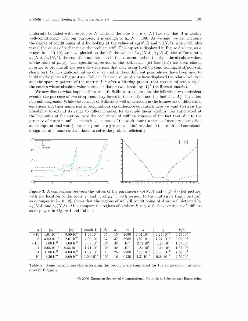
uniformly bounded with respect to N while in the case 3 it is O(N) (we say that A is weaklywell-conditioned). For our purposes, it is enough to fix N = 100. As we said, we can measurethe degree of conditioning of A by looking at the values of κd(N, δ) and γd(N, δ), which will alsoreveal the values of α that make the problem stiff. This aspect is displayed in Figure 3 where, as αranges in [−10, 10], we have plotted on the left the values of κd(N, δ), γd(N, δ), the stiffness ratioκd(N, δ)/γd(N, δ), the condition number of A in the ∞-norm, and on the right the absolute valuesof the roots of pα(z). The specific expression of the coefficient c(α) (see (14)) has been chosenin order to provide all the possible situations that may occur (well/ill conditioning, stiff/non-stiffcharacter). Some significant values of α, related to these different possibilities, have been used tobuild up the plots in Figure 4 and Table 2. For each value of α we have displayed the related solutionand the sparsity pattern of the matrix A−1 after a filtering process that consists of removing allthe entries whose absolute value is smaller than ε (we denote by A−1

f the filtered matrix).We now discuss what happens for α = −10. Stiffness translates into the following two equivalent

events: the presence of two steep boundary layers in the solution and the fact that A−1f has a few

non null diagonals. While the concept of stiffness is well understood in the framework of differentialequations and their numerical approximations via difference equations, here we want to stress thepossibility to extend its range to different areas, for example linear algebra. As anticipated atthe beginning of the section, here the occurrence of stiffness consists of the fact that, due to thepresence of essential null elements in A−1, most of the work done (in terms of memory occupationand computational work), does not produce a great deal of information in the result and one shoulddesign suitable numerical methods to solve the problem efficiently.

−10 −5 0 5 1010−5

100

105

1010

1015

kγk/γcond(A)

−10 −9 −8 −7 −6 −5 −4 −3 −2 −1 0 1 2 3 4 5 6 7 8 9 100

1

2

3

4

5

6

7

8

9

10|z

1|

|z2|

Figure 3: A comparison between the values of the parameters κd(N, δ) and γd(N, δ) (left picture)with the location of the roots z1 and z2 of pα(z) with respect to the unit circle (right picture),as α ranges in [−10, 10], shows that the regions of well/ill conditioning of A are well detected byκd(N, δ) and γd(N, δ). Also, compare the regions of α where k � γ with the occurrence of stiffnessas displayed in Figure 4 and Table 2.

α |z1| |z2| cond(A) d1 d2 m k γ k/γ

−10 1.01 10−1 9.89 100 1.49 100 15 15 2690 1.01 10−1 2.24 10−3 4.49 101

−3 3.82 10−1 2.61 100 4.99 100 37 37 5968 3.82 10−1 1.24 10−2 3.09 101

−1.5 1.00 100 1.00 100 3.63 102 102 102 104 2.77 100 1.76 100 1.57 100

1 8.66 10−1 8.66 10−1 1.71 107 102 102 104 1.84 106 1.14 105 1.62 101

4 0.00 100 4.00 100 1.67 100 1 25 2200 2.50 10−1 3.33 10−3 7.50 101

10 1.39 100 8.60 100 1.09 1015 102 16 6430 2.31 1014 9.24 1012 2.50 101

Table 2: Some parameters characterizing the problem are compared for the same set of values ofα as in Figure 4.



0 20 40 60 80 100−1

−0.5

0

α=−1

0

0 50 100

0

50

100

0 20 40 60 80 100−1

−0.5

0

α=−3

0 50 100

0

50

100

0 20 40 60 80 100−5

0

5

α=−1

.5

0 50 100

0

50

100

0 20 40 60 80 100−2

0

2x 106

α=1

0 50 100

0

50

100

0 20 40 60 80 100−1

−0.5

0

0.5

α=4

0 50 100

0

50

100

0 20 40 60 80 100−5

0

5x 1014

α=10

0 50 100

0

50

100

Figure 4: For α ∈ {−10,−3,−1.5, 1, 4, 10}, we report a plot of the solution y (columns 1 and 3)together with a visualization of the sparsity pattern of the matrix A−1

f (columns 2 and 4). It isworth noting that the appearance of strong layers in the solution corresponds to the case whereA−1f is banded. The pictures should be viewed in combination with Table 2.

5.1 Well conditioning of a one parameter family of Toeplitz matrices

The results of the above examples can be generalized to banded N × N Toeplitz matrices, withk1 lower diagonals and k2 upper diagonals. Such a matrix is well conditioned if the roots of itsassociated polynomial are such that k1 of them are inside and k2 are outside the unit disk (see[2, 5] for more details). The analysis of the stability properties of numerical methods for ODEsrequires the study of the conditioning of Toeplitz matrices depending on a complex parameter.This is done by considering the conditioning in a region of the complex plane. Consider the matrixA of Example 5.2, and take α = a−λ, with a ∈ R and λ ∈ C. By setting T = A+λI, the problembecomes (T − λI)y = b. Now, the roots of the polynomial p(z)− λz = γz2 + (a− λ)z + β depend

on the complex parameter λ. In correspondence of the values of λ such that(z2(λ)z1(λ)

)N= 1 the

solution does not exist: such values are the eigenvalues of T.

Now, suppose we want the system to be well conditioned for all values of λ in a given region,for example C−. This means that for all λ ∈ C− the two roots need to be such that one is insideand the other is outside the unit circle. Suppose that it is known that for a value λ∗ ∈ C− theroots are such that one is inside and the other is outside the unit disk; by exploiting a continuityargument, the best way to check whether the two roots remain in the same position with respectto the unit disk is to monitor if they cross the unit circle for λ ∈ C−. This leads us to consider

Γ ={λ(θ) ≡ p(eiθ)

eiθ, 0 ≤ θ ≤ 2π

}, which is referred to as the boundary locus and is the locus of the

values of λ where one or both of the roots z1(λ), z2(λ) cross the unit circle. Of course, if such acurve completely lies in C+, then the matrix T − λI will be well conditioned in C−. In Figure 5 atypical boundary locus is represented. Note that the eigenvalues are all inside the region boundedby Γ.

The matrix is well conditioned in a region D if there exists λ∗ ∈ D such that T = A + λ∗Iis well conditioned, and D

⋂Γ = ∅. If λ ∈ ∂Γ, i.e. if it is allowed for some roots to be on the

unit circle, then the matrix is weakly well conditioned. In the latter case the condition numbergrows polynomially. Special importance arises when the roots of unit modulus are simple, i.e. thecondition number grows linearly.



0 0.5 1 1.5 2 2.5 3−2

−1.5

−1

−0.5

0

0.5

1

1.5

2BC with eigenvalues

real(λ)

imag

(λ)

Figure 5: Typical boundary locus. The eigenvalues are the points inside.

Generalizations to more general banded Toeplitz matrices are easily obtainable. Let TN =AN − qBN , and assume that

- AN and BN are banded Toeplitz matrices;

- k + 1 is the maximum value of the bandwidth of TN .

- ρ(z) and σ(z) are the two representative polynomials of AN and BN respectively, both ofdegree k;

- q ∈ D ⊂ C;

- π(z, q) = ρ(z)− qσ(z);

- Γ = {q(θ) = ρ(eiθ)σ(eiθ)

), 0 ≤ θ < 2π};

- k1 is the number of lower diagonals and k2 the number of upper diagonals of TN .

Then, the more general form of the root condition is as in the following theorem [5].

Theorem 5.3 The N × N banded Toeplitz matrix TN is well conditioned in a region D of thecomplex plane, i.e. cond(TN − λIN ) is independent of N for all q ∈ D, if there exists q∗ ∈ D suchthat TN (q∗) is well conditioned, and Γ

⋂D = ∅.

It is worth stressing here the convenience of using the position of the roots with respect tothe unit circle as compared to the more popular use of the localization of the eigenvalues of thematrices TN . In fact, when N is large, the latter are not enough to describe the conditioning ofthe Toeplitz matrices. New entries such as quasi-eigenvalues or pseudo-spectrum need to be takeninto account. On the contrary, the boundary locus is defined in a simple algebraic way and oftenits position can be obtained in a relatively easy manner (see, e.g.[5]). To be more clear, referring



to Figure 5, the pseudo-spectrum is the interior part of the bounded region of the complex planesurrounded by Γ deprived of the eigenvalues. In other words, Γ is a sort of Pandora’s box: all thevalues of q where T (q) is singular or ill conditioned are inside of it2.

5.2 Stability of Linear Multistep Methods

Let y0, y1, . . . , yk1−1 be the initial data and yN+k1+1, yN+k1+2, . . . , yN+k1+k2be the final data. A

LMM applied to the test equation (11) with the above boundary conditions leads to the discreteproblem

(AN − qBN )yN = b,

where AN and BN are Toeplitz matrices having k1 lower non zero diagonals and k2 upper non zerodiagonals. The case k2 = 0 corresponds to the classical choice of using discrete IVPs.

The non zero entries of the matrix A are the coefficients of the polynomial ρ, while those of Bare the coefficients of the polynomial σ. To the matrix CN (q) = AN − qBN we may apply eitherthe generalized root condition or the boundary locus condition. The representative polynomial isnow π(z, q) = ρ(z)−qσ(z). The matrix CN will be well conditioned if k1 roots are inside and k2 areoutside the unit disk. The convergence is ensured if Γ is a Jordan curve (this will prevent havingdouble roots on the unit circle) and 0 ∈ Γ.

The extension of the theory to the discretization of continuous BVPs is made without difficulty.If the choice k2 = 0 is made, in order to have the discrete problem asymptotically stable in a

non empty region of the negative half plane, the polynomial π(z, q) = ρ(z)− qσ(z) needs to haveall the roots inside the unit circle for q in a non empty region D of the complex plane. The caseD k C− is the most interesting (A−stability).

The request is however conflicting with the order conditions, as established by the Dahlquistbarrier [11]. If, however, the additional conditions are split, i.e. part of them, say k1 are imposedat the beginning of the interval and part, say k2, at the end of the integration interval, then theconflict disappears. The discrete problem becomes a boundary value one.

Example 5.4 (Midpoint method) The midpoint rule applied to the test equation, yn+1 =yn−1 + 2qyn, may generate two different discrete methods: the classical one where the additionalcondition is y1, and the Boundary Value Method (BVM) where the additional condition is yN+1.In the first case the matrix CN (q) is

C(1)N (q) =

1−q 1−1 −q 1

. . .. . .

. . .

. . .. . .

. . .

N×N

,

while in the second case it is

C(2)N (q) =

−q 1−1 −q 1

−1 −q 1. . .

. . .. . .

N×N

.

2The only thing wrong with this metaphor is that, according to the usual convention in complex analysis, thepart of the two regions defined by Γ where T (q) is ill conditioned is the external one which, for the example reportedin Figure 5, coincides with the bounded region.



The representing polynomial π(z, q) = z2 − 2qz − 1 is the same in the two cases but the firstmatrix has two lower diagonals, while the second has only one. Except for the values of q onthe segment I = (−i, i), the roots of π(z, q) are always one outside and one inside the unit disk.

This implies that the matrix C(2)N is well conditioned for q ∈ C\I and weakly well conditioned for

q ∈ I. Concerning the value of the conditioning parameters, trivially κc ' 1 for <(λ) < 0 andκc ' e<(λ)T for <(λ) > 0. For the second discrete problem we have κd ' |z1|0 ≤ 1 for <(q) ∈ C\I.The continuous problem is then not well represented by the BVM midpoint method for <(q) > 0,and never well represented by the IVM midpoint for q 6= 0.

As far as dissipative problems are considered, i.e. problems having asymptotically stable equi-libria, it is not important that the continuous problem is not well represented in C+. In othercases, for example for conservative systems, it may be important that the continuous problem iswell represented in all of C. A necessary condition for this is that the boundary locus coincideswith the imaginary axis. Methods showing such a property are usually called perfectly stable. Asan example of perfectly stable methods we present the methods having the highest order allowedto a k step formula.

Example 5.5 (Top Order Methods) The methods having the highest order of convergencehave been studied by Dahlquist in [13]. They were proved to be unstable (i.e. not 0− stable)and then not even convergent. If instead we define the correct discrete boundary value problemsthey are however convergent. In [5, sections 4.4, 4.5] the convergence theorem was generalized inorder to include such methods as well. The sufficient conditions for convergence are:

1. consistency;

2. the roots of the polynomial ρ(z) must satisfy the condition (0k1,k2stability)

|z1| ≤ |z2| ≤, . . . |zk1| ≤ 1 < |zk1+1| ≤ . . . ≤ |zk1+k2

|,

being simple the roots of unit modulus.

The second condition is equivalent to asking that the matrix AN is weakly well conditioned.Concerning the polynomial p(z, q) = ρ(z)− qσ(z), it turns out that when k = 2ν + 1, it has ν + 1roots inside and ν roots outside the unit disk, for all q ∈ C−. The boundary locus is the imaginaryaxis (see [5, 1] ).

6 Solution of Linear Systems

It is well known that iterative methods for the solution of linear systems Ax = b fit very well intothe framework of AS dynamical systems. Infact the splitting technique is nothing but a strategy totransform the solution y = A−1b into the AS equilibrium point of an appropriate linear dynamicalsystem. What is usually less emphasized is that even in the so called direct methods the AS playa central role, not only when dealing with structured matrices (as seen in section 5), but also inthe more general case. Hereafter we give an example of the use of the conditioning parameters inan unusual setting, i.e. not deriving from a differential problem.

Example 6.1 LU factorization Let A be a real N ×N matrix. Consider the sequence

A0 = A, AN = IN

Aj = L−1j Aj−1U

−1j , j = 1, N ;



where

Lj =

Ij−1

1a−1j sj IN−j

, Uj =

Ij−1

aj tTjIN−j

, Aj =

Ij−1

1QN−j

,

with sj and tj appropriately defined vectors. The final matrix is IN . The matrices L =∏j=1,N−1 Lj

and U =∏j=1,N−1 UN−j , for j = 1, N − 1 define the LU factorization of A.

We would like to study the stability of the algorithm performed in finite precision arithmetic. Herethe dynamics is not uniquely defined in that there is a certain freedom in the choice of both Ljand Uj . One is able to maintain the entries of Lj to be small by the pivoting strategy, but still theentries of Aj and consequently Uj may grow. For simplicity we suppose that A has already beenpermuted so that no row pivoting is necessary. Parameters which monitor how the perturbationintroduced by the floating point arithmetic change the initial data in a backward error analysis,called growth factors, have been defined by Wilkinson and more recently by Amodio and Mazzia[3]. When such parameters grow exponentially with N the problem is said to be unstable. Acomputation of the parameter κd for this problem yields

κd =maxj=1,...,N ‖Aj‖∞

‖A‖∞,

and this is essentially the same value of the growth factor ρ defined in [3].

7 Conclusions

We have analyzed the differences between two key concepts in NA, i.e. stability and conditioning,as well as the relations between the specific use of the term stability in NA and the same term usedin other fields of Mathematics. The notion of conditioning appears to be more general than thatof stability, and potentially able to settle in a unified framework all sensitivity problems arisingin NA. In order to support and elucidate this point of view, we have introduced two parametersthat measure the conditioning of a problem using two different norms. The information providedby them allowed us to redefine the classical notion of stiffness for ODEs and extend it to otherbranches of NA and in particular numerical linear algebra. An interesting and curious result wasthat a “stiff” Toeplitz banded matrix is a matrix whose inverse is still a banded matrix (up to themachine precision).

Acknowledgement.

Work supported by GNCS-INDAM and Italian MIUR.

References

[1] L. Aceto, R. Pandolfi, D. Trigiante, One Parameter Family of Linear Difference Equationsand the Stability Problem for the Numerical Solution of ODEs, In press.

[2] P. Amodio, L. Brugnano, The conditioning of Toeplitz band matrices, Mathematical and Com-puter Modelling 23, No. 10 (1996), 29–42.

[3] P. Amodio, F. Mazzia, A new Approach to Backward Error Analysis of LU Factorization, BIT39 (1999), 385–402.



[4] L. Brugnano and D. Trigiante, A new mesh selection strategy for ODEs, Appl. Numer. Math.,24 No. 1 (1997), 1–21.

[5] L. Brugnano, D. Trigiante, Solving Differential Problems by Multistep Initial and BoundaryValue Methods, Gordon & Breach, 1998.

[6] L. Brugnano, D. Trigiante, On the characterization of stiffness for ODEs, Dynamics of Con-tinuous, Discrete and Impulsive Systems, 2 (1996), 317–335.

[7] J. R. Cash, A Note on the Numerical Solutions of Linear Recurrence Relations, Num. Math34 (1981), 371–386.

[8] J. R. Cash, An extension of Olver’s method for the numerical solution of linear differenceequations, Math Comp. 32 (1978), 497–510.

[9] J. R. Cash, Stable Recursions, Academic Press, London, 1979.

[10] J. R. Cash and F. Mazzia, A new mesh selection algorithm, based on conditioning, for two-point boundary value codes, J. Comput. Appl. Math., 184(2) (2005), 362–381.

[11] G. Dahlquist, A special stability problem for linear multistep methods, BIT 3 (1963), 27–43.

[12] G. Dahlquist, 33 Years of Numerical Instability, Part I, BIT 25 (1985), 188–204.

[13] G. Dahlquist, Convergence and stability in the numerical integration of ordinary differentialequations, Math Scan. 4 (1956), 33–53.

[14] W. Gautschi, Computational Aspects of three-terms Recurrence Relations, SIAM Rev. 9(1967), 24–82.

[15] F. Iavernaro, F. Mazzia and D. Trigiante, Eigenvalues and quasi-eigenvalues of banded Toeplitzmatrices: some properties and applications, Numerical Algorithms 31(1-4) (2002), 157–170.

[16] V. Lakshmikantham, D. Trigiante, Theory of Difference Equations, Numerical methods andApplications, Second Edition, Marcel Dekker, New York, 2002.

[17] P. Lax, R. D. Richtmyer, Survey of the Stability of Linear Finite Difference Equations, PartI, Comm. on Pure and Appl. Math. IX (1956), 267-293.

[18] F. Mazzia and D. Trigiante. A hybrid mesh selection strategy based on conditioning for bound-ary value ODE problems, Numer. Algorithms, 36(2) (2004), 169–187.

[19] J. M. Ortega, Stability of difference equations and convergence of iterative processes, SIAM J.Numer. Anal. 10 (1973), 268–282.

[20] F. W. J. Olver, Numerical Solutions of Second Order Linear Difference Equations, J. Res.N.B.S. 71B (1967) 111–129.

[21] F. W. J. Olver, Error bounds for Linear Recurrence Relations, Math. Comp. 60 (1988), 481–499.

[22] J. C. P. Miller, Bessel functions, Part II, Math. Tables, vol. X, British Association for theAdvancement of Sciences, Cambridge University Press, 1952.

[23] A. M. Stuart, A. R. Humphries, Dynamical Systems and Numerical Analysis, CambridgeUniversity Press, 1966.



[24] L. N. Trefethen, M. Embree, Spectra and pseudospectra. The behavior of nonnormal matricesand operators, Princeton University Press, Princeton, NJ, 2005.

[25] R. V. M. Zahar, Mathematical analysis of Miller’s algorithm, Num. Math., 27 (1977), 427–447.


Stability and conditioning in numerical analysis

Documents

Transcript of Stability and conditioning in numerical analysis