water

Article

SPI Drought Class Predictions Driven by the NorthAtlantic Oscillation Index Using Log-Linear Modeling

Elsa E. Moreira 1,*, Carlos L. Pires 2 and Luís S. Pereira 3

1 Center of Mathematics and Applications (CMA), Faculty of Sciences and Technology,New University of Lisbon, Caparica 2829-516, Portugal

2 Instituto Dom Luiz (IDL), Faculty of Sciences, University of Lisbon, Lisboa 1749-016, Portugal;clpires@fc.ul.pt

3 Research Center for Landscape, Environment, Agriculture and Food (LEAF), Institute of Agronomy,University of Lisbon, Lisbon 1349-017, Portugal; lspereira@isa.ulisboa.pt

* Correspondence: efnm@fct.unl.pt; Tel.: +351-212-948-300 (ext. 10867)

Academic Editor: Athanasios LoukasReceived: 13 October 2015; Accepted: 27 January 2016; Published: 30 January 2016

Abstract: This study aims at predicting the Standard Precipitation Index (SPI) drought classtransitions in Portugal, considering the influence of the North Atlantic Oscillation (NAO) as one of themain large-scale atmospheric drivers of precipitation and drought fields across the Western Europeanand Mediterranean areas. Log-linear modeling of the drought class transition probabilities on threetemporal steps (dimensions) was used in an SPI time series of six- and 12-month time scales (SPI6 andSPI12) obtained from Global Precipitation Climatology Centre (GPCC) precipitation datasets with1.0 degree of spatial resolution for 10 grid points over Portugal and a length of 112 years (1902–2014).The aim was to model two monthly transitions of SPI drought classes under the influence of the NAOindex in its negative and positive phase in order to obtain improvements in the predictions relative tothe modeling not including the NAO index. The ratios (odds ratio) between transitional probabilitiesand their confidence intervals were computed in order to estimate the probability of one droughtclass transition over another. The prediction results produced by the model with the forcing of NAOwere compared with the results produced by the same model without that forcing, using skill scorescomputed for the entire time series length. Overall results have shown good prediction performance,ranging from 73% to 76% in the percentage of corrects (PC) and 56%–62% in the Heidke skill score(HSS) regarding the SPI6 application and ranging from 82% to 85% in the PC and 72%–76% in theHSS for the SPI12 application. The model with the NAO forcing led to improvements in predictionsof about 1%–6% (PC) and 1%–8% (HSS), when applied to SPI6, but regarding SPI12 only seven of thelocations presented slight improvements of about 0.4%–1.8% (PC) and 0.7%–3% (HSS).

Keywords: 3-dimensional log-linear models; drought class transitions; odds; confidence intervals

1. Introduction

Drought is a natural temporary imbalance of water availability, consisting of a persistentlower-than-average precipitation, of uncertain frequency, duration and severity, and of unpredictableor difficult-to-predict occurrence, resulting in diminished water resource availability and carryingcapacity of ecosystems [1]. The importance of early warning to water users for timely implementationof preparedness and mitigation measures is well known and has been widely addressed by severalauthors [1–3]. Developing prediction tools appropriate for the climatic and agricultural conditionsprevailing in different drought-prone areas constitutes a research challenge. Drought prediction isa major concern for water managers, farmers and other water end-users because it constrains theirdecisions. Since droughts have a slow initiation, it is possible to release a timely prediction so that

Water 2016, 8, 43; doi:10.3390/w8020043 www.mdpi.com/journal/water

Water 2016, 8, 43 2 of 18

measures and policies can be taken in order to mitigate the effects of the drought [3,4]. Short-termdrought predictions, from one to three months, may be used to alert farmers and water managersabout the initiation, continuation or end of a drought and about the need for preparedness measuresbefore a drought is effectively installed or for a post-drought period. However, forecasting when adrought is likely initiating or to coming to an end is a difficult task.

Drought severity is usually identified through indices such as the Standardized Precipitation Index(SPI), the Palmer Drought Severity Index (PDSI) and the MedPDSI [5–7]. However, in the InterregionalWorkshop on Indices and Early Warning Systems for Drought 2009, several organizations, including theWorld Meteorological Organization (WMO) and the United States National Oceanic and AtmosphericAdministration (NOAA), recommended that the SPI be used by all national meteorological andhydrological services around the world to characterize meteorological droughts as well as agriculturaland hydrological droughts because the SPI is an index that is simple to understand, is easy to calculateand is statistically relevant and meaningful [8]. In fact, precipitation is the only required inputparameter and it considers in its conception the different impacts on groundwater, reservoir storage,soil moisture, snowpack and stream-flow through the different time scales of computation [5,8].The SPI is based on the probability of precipitation for any time scale. The probability of observedprecipitation is then transformed into an index that supports assessing drought severity and mayprovide early warning of drought.

The precipitation occurrence and/or its inhibition leading to drought on different time and spatialscales is driven by atmospheric forcings which may range from the mesoscale (hundreds of km) upto the planetary scale (tens of thousands of km). The large-scale atmospheric state may roughly bedescribed by a time-varying state vector filled with a few numbers of leading principal componentsof the sea-level pressure (SLP) field. That state vector either exhibits a transient behavior or persistsnear certain states, the so-called weather regimes (WRs) or atmospheric circulation patterns, whichare detectable by cluster analysis [9]. Therefore, the projection or pattern correlation of the SLP fieldonto the main WRs acts as large-scale atmospheric circulation indices, which are useful indicatorsof the rainfall field. In particular, several large-scale indices of the Euro-Atlantic and NorthernHemisphere SLP field [10,11] are well correlated with the cumulated precipitation in certain targetregions, namely Portugal [12]. We recall the main four Euro-Atlantic atmospheric WRs as: (1) theblocking regime, with a large anomalous high pressure over Scandinavia; (2) the zonal regime (positivephase of the North Atlantic Oscillation: NAO+), characterized by an intense zonal flow crossingthe North Atlantic area, reinforcing the Icelandic low and the Azores’ high pressure centers; (3) theAtlantic Ridge regime, exhibiting a positive anomaly over the North Atlantic and low pressure overnorthern Europe; and (4) the Greenland anticyclone pattern (negative phase of the North AtlanticOscillation: NAO´), showing a strong positive pressure anomaly centered over western Greenland.Since some of the WRs display nearly symmetric anomalies, the corresponding projections of the SLPfield are not independent. The overall main features of the Euro-Atlantic large-scale atmosphericfield are then well captured by a set of large-scale indices: the North Atlantic Oscillation (NAO)index [13], the EAP (East-Atlantic Pattern) index, the SCAND (Scandinavian Pattern) index [14] andthe East-Atlantic Western Russia (EAWR) index, all available at the National Centers for EnvironmentalPrediction (NCEP) website.One of the main patterns governing wet and dry rainfall regimes in mostof Europe is the NAO [14]. The NAO index is commonly given by the difference in normalizedSLP anomalies between a southern node, located in continental Iberia or the Azores, and a northernnode, usually in southwest Iceland [13,15]. Strong positive phases of the NAO (i.e., NAO+) tendto be associated with above-average temperatures in the eastern United States and across northernEurope and below-average temperatures in Greenland and oftentimes across southern Europe andthe Middle East. The NAO+ regime is also associated with above-average precipitation over northernEurope and Scandinavia in the winter, and below-average precipitation or drought over southern andcentral Europe, Mediterranean regions and the north of Africa. Opposite patterns of temperature and

Water 2016, 8, 43 3 of 18

precipitation anomalies are typically observed during strong negative phases of the NAO available atthe National Centers for Environmental Prediction (NCEP) website.

Pires and Perdigão [16] have shown high levels of correlation between the NAO index and theSPI reaching the negative value ´0.60 for the winter months for some locations in northern Portugal,which convert the NAO in an interesting tool for the improvement of drought predictions. The NAOinfluences on the precipitation regimes and droughts in Portugal and the Iberian Peninsula are alsoreported by other researchers [17,18]. Santos et al. [12] have shown that dry weather conditions prevailwhen the NAO index is positive (NAO+). The drought frequency in Portugal has been increasing as aconsequence of a drying signal in the Mediterranean region attributable to a trend in the atmosphericcirculation forcing, namely a decadal scale enhancement of the positive phase of the North AtlanticOscillation [19].

Several statistical and physical-based techniques as well as the combination of both (hybridtechniques) have been proposed for the forecasting of droughts and the cumulated precipitation ona monthly basis. The state-of-the-art physical models used for weather and climate prediction suchas that of the European Center for Medium Range Weather Forecasts (ECMWF) have been used forobtaining probabilistic ensemble-based forecasts up to six months in advance of the SPI worldwideon scales of three, six and 12 months [20]. Since the computational burden of those predictions isvery high and they depend on the availability of a physical model, a reasonable alternative for themeteorological community started by developing simple statistical models of the monthly and seasonalcumulated precipitation [21,22]. Those models often apply multivariate statistical techniques suchas the Canonical Correlation Analysis (CCA), robust multilinear regression, and Singular SpectrumAnalysis (SSA), among others [23], and they rely on a set of previously well-chosen physical predictorsthat are able to capture the main boundary layer’s forcing of the atmospheric dynamics (e.g., the seasurface temperature (SST), the snow cover and land moisture fields) and the intrinsic predictablefeatures such as the internal (not externally forced) oscillations of the climatic system. In regardto hybrid predictions, we must refer to several techniques. On one hand, we have the mixing byBayesian probabilistic averaging, either of different physical-based predictions [24] or of physical andstatistical models [25]. On the other hand, we may use the optimal regression of physical precursorsand dynamical forecasts of drought indices [26].

Hereby we will focus on statistical methods of drought prediction only. Combining the stochasticproperties of the SPI with weather pattern indices such as NAO is a challenge for the short-termprediction of droughts by statistical methods. The stochastic properties of the SPI time series havebeen explored for analyzing and predicting drought class transitions in the Portuguese context [27–32].

The methodologies include regression analysis [33], time series modeling such as ARIMA andseasonal ARIMA [34,35], artificial neural network models (ANN) [36,37] and stochastic and probabilitymodels such as Markov chains [38–40], log-linear models [31,41] and others [42,43]. Also, hybridmodels combining two techniques have been used, for instance wavelet transforms and neuralnetworks [44], stochastic and neural network modeling [45], wavelet and fuzzy logic models [46],adaptive neuro-fuzzy inference [47] and data mining and ANFIS techniques [48]. Each methodology,independently of its complexity, has advantages and limitations. Mishra and Singh [49] recentlyreviewed and discussed the methodologies used so far for drought modeling.

Approaches to drought forecasting using drought indices associated with atmospheric-oceanicanomaly indices have been suggested for predictions on monthly and seasonal scales. Examplesinclude the use of artificial neural networks and time series of drought indices additionally drivingthe NAO index [37], and the use of probabilistic models that result from evaluating conditionalprobabilities of future SPI classes with respect to current SPI and NAO classes [43].

Three-dimensional (3D) log-linear models allow modeling the state of a variable at time t + 1knowing its state at time t and t ´ 1 [50]. Those models were used to predict SPI drought classtransitions one and two months ahead, knowing the drought class of the last two months [31]. In thisapproach, log-linear models are fitted to 3D contingency tables of drought class transitions counts,

Water 2016, 8, 43 4 of 18

corresponding to two time-step transitions relative to the SPI drought classes at months t ´ 1, t andt + 1 obtained from categorical time series of SPI drought classes. Then, ratios of expected frequencies(odds) relative to the most probable transition for the next month and their confidence intervals arecomputed. This approach allows predictions with a leading time of two or more months and hasshown potential to be improved, namely with the inclusion of new categories in the contingency tables.Recently, the introduction of a new variable representing the wet or the dry season of the year wastested in order to improve the predictions [41].

Considering the advances in drought predictions reviewed above and the reported NAO influenceon precipitation and drought in Portugal, the objectives of this work consist of improving log-linearmodeling of the SPI drought class transitions when driven by the negative or positive phases of theNAO index. This approach is an advance relative to the previous study [31] since it was based uniquelyon the assessment of SPI drought classes. In the current study, long series of monthly precipitation ofmore than 100 years were used, which brings advantages in model-fitting and allows better estimatesfor the transition probabilities.

2. Materials and Methods

2.1. Data, SPI and NAO

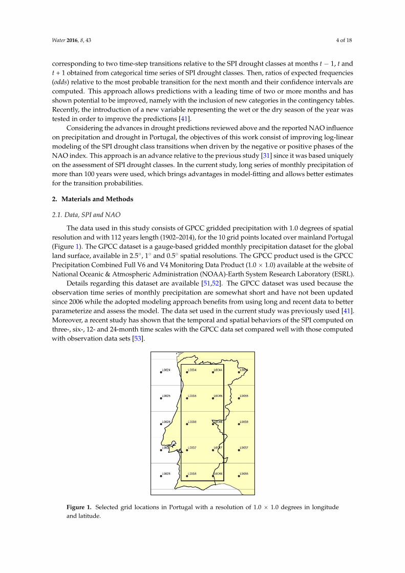
The data used in this study consists of GPCC gridded precipitation with 1.0 degrees of spatialresolution and with 112 years length (1902–2014), for the 10 grid points located over mainland Portugal(Figure 1). The GPCC dataset is a gauge-based gridded monthly precipitation dataset for the globalland surface, available in 2.5˝, 1˝ and 0.5˝ spatial resolutions. The GPCC product used is the GPCCPrecipitation Combined Full V6 and V4 Monitoring Data Product (1.0 ˆ 1.0) available at the website ofNational Oceanic & Atmospheric Administration (NOAA)-Earth System Research Laboratory (ESRL).

Details regarding this dataset are available [51,52]. The GPCC dataset was used because theobservation time series of monthly precipitation are somewhat short and have not been updatedsince 2006 while the adopted modeling approach benefits from using long and recent data to betterparameterize and assess the model. The data set used in the current study was previously used [41].Moreover, a recent study has shown that the temporal and spatial behaviors of the SPI computed onthree-, six-, 12- and 24-month time scales with the GPCC data set compared well with those computedwith observation data sets [53].

Water 2016, 8, 43 4 of 18

improved, namely with the inclusion of new categories in the contingency tables. Recently, the introduction of a new variable representing the wet or the dry season of the year was tested in order to improve the predictions [41].

Considering the advances in drought predictions reviewed above and the reported NAO influence on precipitation and drought in Portugal, the objectives of this work consist of improving log-linear modeling of the SPI drought class transitions when driven by the negative or positive phases of the NAO index. This approach is an advance relative to the previous study [31] since it was based uniquely on the assessment of SPI drought classes. In the current study, long series of monthly precipitation of more than 100 years were used, which brings advantages in model-fitting and allows better estimates for the transition probabilities.

2. Materials and Methods

2.1. Data, SPI and NAO

The data used in this study consists of GPCC gridded precipitation with 1.0 degrees of spatial resolution and with 112 years length (1902–2014), for the 10 grid points located over mainland Portugal (Figure 1). The GPCC dataset is a gauge-based gridded monthly precipitation dataset for the global land surface, available in 2.5°, 1° and 0.5° spatial resolutions. The GPCC product used is the GPCC Precipitation Combined Full V6 and V4 Monitoring Data Product (1.0 × 1.0) available at the website of National Oceanic & Atmospheric Administration (NOAA)-Earth System Research Laboratory (ESRL).

Details regarding this dataset are available [51,52]. The GPCC dataset was used because the observation time series of monthly precipitation are somewhat short and have not been updated since 2006 while the adopted modeling approach benefits from using long and recent data to better parameterize and assess the model. The data set used in the current study was previously used [41]. Moreover, a recent study has shown that the temporal and spatial behaviors of the SPI computed on three-, six-, 12- and 24-month time scales with the GPCC data set compared well with those computed with observation data sets [53].

Figure 1. Selected grid locations in Portugal with a resolution of 1.0 × 1.0 degrees in longitude and latitude.

SPI values on a six-month (SPI6) and 12-month time scale (SPI12) were computed for the 10 precipitation time series referred above. The SPI12 is more appropriate to identify dry and wet periods of relatively long duration and relates better with impacts of drought on the hydrologic

Figure 1. Selected grid locations in Portugal with a resolution of 1.0 ˆ 1.0 degrees in longitudeand latitude.

Water 2016, 8, 43 5 of 18

SPI values on a six-month (SPI6) and 12-month time scale (SPI12) were computed for the10 precipitation time series referred above. The SPI12 is more appropriate to identify dry and wetperiods of relatively long duration and relates better with impacts of drought on the hydrologicregimes [54]. Shorter time scales of six months or less are likely more useful to detect agriculturaldroughts, reflecting a better change of class instead of its persistence [54].

Categorical time series of monthly drought classes were computed based on Table 1, relative toboth SPI6 and SPI12 time series; however, the severe and extremely severe drought classes in Table 1were grouped because transitions referring to the extremely severe drought classes are much lessfrequent than those for other classes, therefore avoiding too many zeros in the contingency tables thatmay cause problems in the fitting.

Table 1. Drought class classification of SPI (modified from MCKEE et al. [55]).

Code Drought Classes SPI Values

1 Non-drought SPI ě 02 Near normal ´1 < SPI < 03 Moderate ´1.5 < SPI ď ´14 Severe/Extreme SPI ď ´1.5

Monthly tabulated NAO indices, based on a Principal Component Approach of the Sea LevelPressure field and dating back to 1950, are available from the National Centers for EnvironmentalPrediction (NCEP) Climate Prediction Center. However, in order to cover the full period ofthe precipitation data (1902–2014), we used an extended historical record (starting in 1864) of astation-based NAO index relying upon the difference of normalized SLP between Lisbon (Portugal)and Reykjavik (Iceland).

Before moving on to modeling, a correlation study was performed in order to find the lag betweenthe NAO index and SPI time series that maximizes the correlation between them both. The Pearsoncorrelation coefficient was computed between the monthly NAO index and the SPI6 and SPI12 timeseries for each grid location and a lag of five months for the SPI6 and 11 months for the SPI12 wasfound. In both cases, these lags indicate that the largest influence of NAO occurs near the startingmonth of the precipitation accumulation period for the SPI which is explained by the large memory ofthe NAO index and the contemporaneous (no lag) large correlation between monthly precipitationand the NAO index [16]. For the purposes of this modeling, when the NAO index for a given month isequal or greater than zero, then the NAO state in that month is positive, otherwise it is negative.

2.2. Modeling

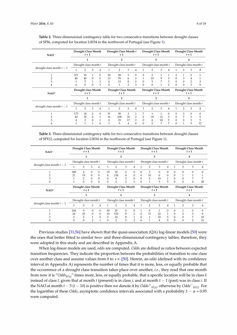
For modeling purposes, the number of two-step monthly transitions between any SPI droughtclass was counted separately for the negative and positive NAO state to form two three-dimensional(4 ˆ 4 ˆ 4) contingency tables [50] with N = 64 cells each. These two contingency tables for NAO´ andNAO+ have three categories: the drought class at month t ´ 1, t and t + 1 with four levels for each one(drought classes 1, 2, 3, and 4 defined in Table 1). Given the previously mentioned lag between theNAO and the SPI and considering that predictions focus on month t + 1, the NAO index was evaluatedat month t ´ 4 or t ´ 10 which correspond to lags of 5 or 11 months for, respectively, the SPI6 andSPI12. Examples of these contingency tables are presented in Tables 2 and 3 for the SPI6 and SPI12.If the NAO state at month t ´ 4 (t ´ 10) was negative then the transition was counted for the tableNAO´, otherwise it was counted for the table NAO+.

Log-linear modeling input consists of the observed frequency nijk, i, j, k = 1, ..., 4 reported in thecontingency tables (e.g., Tables 2 and 3), which consist of the number of times that in a given monththe drought class i was followed by the drought class j in the next month (one-step transitions) andthen by the drought class k in the month after that (two-step transitions). The model computes theexpected frequency mijk, i, j, k = 1, ..., 4, i.e., the expected value E(nijk) of nijk, i, j, k = 1, ..., 4.

Water 2016, 8, 43 6 of 18

Table 2. Three-dimensional contingency table for two consecutive transitions between drought classesof SPI6, computed for location L0034 in the northwest of Portugal (see Figure 1).

NAO´

Drought Class Montht + 1

Drought Class Month t+ 1

Drought Class Montht + 1

Drought Class Montht + 1

1 2 3 4

drought class month t ´ 1Drought class month t Drought class month t Drought class month t Drought class month t

1 2 3 4 1 2 3 4 1 2 3 4 1 2 3 4

1 271 10 1 0 30 38 3 0 2 2 1 1 3 1 2 12 40 40 0 0 13 70 6 2 1 10 9 3 0 3 4 13 1 5 1 3 0 13 8 0 0 5 7 3 0 0 2 34 6 0 0 3 0 1 3 3 0 0 1 2 0 0 3 9

NAO+Drought class Month

t + 1Drought Class Month

t + 1Drought Class Month

t + 1Drought Class Month

t + 1

1 2 3 4

drought class month t ´ 1Drought class month t Drought class month t Drought class month t Drought class month t

1 2 3 4 1 2 3 4 1 2 3 4 1 2 3 4

1 173 18 2 0 51 38 2 1 7 1 1 0 0 3 0 02 40 35 0 1 16 108 10 2 2 18 12 3 0 7 3 53 4 3 0 1 0 19 17 2 0 6 18 5 0 2 3 54 1 1 1 0 1 5 4 0 0 2 7 7 0 1 5 12

Table 3. Three-dimensional contingency table for two consecutive transitions between drought classesof SPI12, computed for location L0034 in the northwest of Portugal (see Figure 1).

NAO´

Drought Class Montht + 1

Drought Class Montht + 1

Drought Class Montht + 1

Drought Class Montht + 1

1 2 3 4

drought class month t ´ 1Drought class month t Drought class month t Drought class month t Drought class month t

1 2 3 4 1 2 3 4 1 2 3 4 1 2 3 4

1 308 4 0 0 19 18 0 0 0 2 0 0 0 0 0 02 21 19 0 0 4 134 4 0 0 10 6 0 0 1 1 13 1 2 0 0 0 8 3 0 0 0 19 1 0 0 7 74 1 0 0 0 0 2 2 1 0 1 5 5 0 0 4 28

NAO+Drought class Month

t + 1Drought Class Month

t + 1Drought Class Month

t + 1Drought Class Month

t + 1

1 2 3 4

drought class month t ´ 1Drought class month t Drought class month t Drought class month t Drought class month t

1 2 3 4 1 2 3 4 1 2 3 4 1 2 3 4

1 244 9 0 0 30 29 0 0 1 0 1 0 0 1 0 02 24 23 0 0 10 152 8 2 0 17 10 1 0 2 3 03 2 2 1 0 0 14 8 1 0 1 22 5 0 0 7 104 0 0 2 1 0 2 2 2 0 1 4 9 0 0 2 21

Previous studies [31,56] have shown that the quasi-association (QA) log-linear models [50] werethe ones that better fitted to similar two- and three-dimensional contingency tables; therefore, theywere adopted in this study and are described in Appendix A.

When log-linear models are used, odds are computed. Odds are defined as ratios between expectedtransition frequencies. They indicate the proportion between the probabilities of transition to one classover another class and assume values from 0 to +8 [50]. Herein, an odds (defined with its confidenceinterval in Appendix A) represents the number of times that it is more, less, or equally probable thatthe occurrence of a drought class transition takes place over another, i.e., they read that one monthfrom now it is “Oddskl|ij” times more, less, or equally probable, that a specific location will be in class kinstead of class l, given that at month t (present) is in class j, and at month t ´ 1 (past) was in class i. Ifthe NAO at month t´ 5 (t´ 10) is positive then we denote it by Odds`kl|ij, otherwise by Odds´kl|ij. Forthe logarithm of these Odds, asymptotic confidence intervals associated with a probability 1 ´ α = 0.95were computed.

Water 2016, 8, 43 7 of 18

Odds confidence intervals, besides reflecting the sampling variability of the observed droughttransitions internal to each time series, also indicate if a given odds is significantly different from 1.For a 5% significance level, if the confidence interval for an odds includes the value 1, then there isa 95% probability that the odds in fact equals 1, meaning that the drought transition from class i toclass j to class k and the drought transition from class i to class j to class l are not significantly different.Otherwise, there is also a 95% probability that the odds is in fact larger (smaller) than 1, meaning thatthe first transition is significantly more (less) probable than the second. If the confidence interval of agiven odds is too large then the reliability of the prediction is small.

For obtaining the most probable class transition for the month t + 1, the odds for the threeclosest class transitions, starting from the drought class at month t, are computed as well as theirconfidence intervals. The most probable transition is chosen. For instance, if the drought classes atmonth t ´ 1 and t are equal to 3 and 4, respectively, then Odds34|34, Odds24|34 and Odds23|34 will becomputed. If the values and respective confidence intervals obtained for those odds are, for instance,Odds43|34 “ 2.45r1.18, 3.89s, Odds42|34 “ 5.35 r3.92, 8.62s and Odds32|34 “ 1.99 r0.76, 5.01s, then class 4is more probable than class 3 and much more probable than class 2, obviously because a jump from aclass to another with a one-point difference is always more probable than that to a class with two orthree points of difference. At last, class 3 is more probable than class 2, resulting in that class 4 is themost probable for the month t + 1, thus meaning maintenance of the previous class.

2.3. Model Performance

The model performance was assessed using the Heidke skill score (HSS) [23,57]. The HSSmeasures the fractional improvement of the forecast over a random prediction. The range of the HSS is´8 to 1. Negative values indicate that the chance forecast is better than the model prediction, HSS = 0means no skill, while a perfect forecast obtains a HSS of 1. The computation of the HSS involvesbuilding the contingency table presented in Table 4 which is used in HSS and defined as follows:

HSS “

˜

4ÿ

i“1

pii ´

4ÿ

i“1

pi p1i

¸

{

˜

1´4ÿ

i“1

pi p1i

¸

(1)

where pii is the proportion of predictions that agreed with the observations for class i and pik is theproportion of events with predictions at class i and observed at class k with i ‰ k, and pi and p1i are themarginal totals in Table 4. This approach was previously tested [41].

Table 4. Contingency table for the prediction of four drought classes for computing the Heidkeskill score.

Drought Classes Observed

predicted 1 2 3 4 Marginal total1 p11 p12 p13 p14 p'1 = Σp1k2 p21 p22 p23 p21 p'2 = Σp2k3 p31 p32 p33 p34 p'3 = Σp3k4 p41 p42 p43 p44 p'4 = Σp4k

Marginal total p1 = Σpi1 p2 = Σpi2 p3 = Σpi3 p4 = Σpi4 100%

The measure that gives the total number of agreements, called the proportion of corrects (PC), iseasily obtained from Table 4, and is simply given by:

PC “4ÿ

i“1

pii (2)

Water 2016, 8, 43 8 of 18

3. Results and Discussion

Both contingency tables for NAO´ and NAO+, either relative to the SPI6 (Table 2) or the SPI12(Table 3), present higher frequency values for the transitions that imply the maintenance of theprecedent drought classes and smaller frequencies for the transitions that imply the increase/decreaseof the drought classes, particularly when changing by two or three values. As for previousstudies [31,41], this maintenance trend results from the fact that droughts (of six- and 12-monthtemporal scales) install slowly, tend to remain for a relatively long time, and have a slow dissipation.These maintenance characteristics are less evident when using the SPI6 since it responds quickly toincreases or decreases in the precipitation because the computation cumulative period is shorter thanfor SPI12. Data in Tables 2 and 3 show that NAO´ favors the transitions from drought class 1 to itself,i.e., maintaining a non-drought condition, while the NAO+ favors transitions from drought class 3and 4 to themselves, although not significantly, i.e., the maintenance of moderate and severe droughtclasses, particularly when considering the SPI6.

Tables 5 and 6 present results for four out of the 10 locations using, respectively, SPI6 and SPI12data (L0035, L0038, L0045 and L0048). These tables allow us to compare the drought classes “OBS”when calculated from observed data and predicted with the log-linear modeling driven and not drivenby NAO, respectively referred to as “predicted w/NAO” and “predicted”. The period selected for thecomparison, October 2011 to February 2013, refers to a drought event, therefore including its initiation,development and dissipation. For each site, the observed SPI6 (SPI12) drought class at months t ´ 1and t are presented, as well as the classes at month t + 1 “observed” and “predicted w/NAO” and“Predicted”. In addition, the NAO index values at month t ´ 4 (t ´ 10) are also presented. When twoor three drought classes are equally probable, then the predicted drought class is identified as “1 or 2”or “2 or 3 or 4”, for instance, which means that probabilities for the transitions into classes 1 or 2 or intoclasses 2 or 3 or 4 are similar. The cells in Tables 5 and 6 are highlighted in grey when the predictionsdo not match the observations.

Results in Tables 5 and 6 show that the model performs very well in predicting the maintenanceof the drought class, but generally does not perform well when a decrease or increase of the droughtclass category occurs which breaks with the drought class established in the preceding two months.Because of the negative correlation between the NAO index and precipitation in Iberia [12,16,17], thewet and less dry classes, i.e., classes 1 and 2 (see Table 1), tend to occur when the NAO index is negative.However, with the log-linear model driven by NAO, some cases of class change could be predictedbetter, namely those in the negative NAO regime (NAO´) (e.g., 13 February and 12 August for SPI6in L0035), leading to wet conditions in western Iberia. That is because the sensitivity of precipitationto the NAO index is generally stronger in the wetter regimes, in accordance with the asymmetriccorrelations between NAO and SPI presented by Pires and Perdigão [16].

From comparing predictions relative to SPI6 (Table 5) with those of SP12 (Table 6), it couldbe observed that the number of disagreements is large for SPI6. This behavior is likely due to thelarger number of class changes in the case of SPI6, since this index denotes a shorter time span of thecumulated precipitation than SPI12 and therefore produces a quicker response to the variability ofprecipitation which results in more frequent changes of drought classes. Results for the other locationsand for other drought events simulated have shown behaviors similar to those referred above.

Water 2016, 8, 43 9 of 18

Table 5. SPI6: comparison between observed (OBS) and predicted drought class transitions (“Predicted w/NAO” and “Predicted” for four locations during the periodOctober 2011 to February 2013).

L0035 NAO Drought Class at Drought Class at Month t + 1 L0038 Drought Class at Drought Class at Month t + 1

Date Month t ´ 4 Month t ´ 1 Month t OBS Predicted w/NAO Predicted date Month t ´ 1 Month t OBS Predicted w/NAO Predicted

October-2011 ´1.58 3 3 2 2 or 3 or 4 2 or 3 or 4 October-2011 1 1 1 1 1November-2011 ´3.39 3 2 2 1 or 2 2 November-2011 1 1 2 1 1December-2011 ´0.18 2 2 3 2 2 December-2011 1 2 2 2 2January-2012 2.97 2 3 4 2 or 3 or 4 2 or 3 or 4 January-2012 2 2 2 2 2February-2012 1.45 3 4 4 4 4 February-2012 2 2 2 2 2March-2012 0.74 4 4 4 4 4 March-2012 2 2 2 2 2April-2012 3.2 4 4 4 4 4 April-2012 2 2 3 2 2May-2012 2.05 4 4 4 4 4 May-2012 2 3 2 2 or 3 2 or 3June-2012 1.28 4 4 3 4 4 June-2012 3 2 2 2 2July-2012 1.78 4 3 2 2 or 3 or 4 2 July-2012 2 2 2 2 2

August-2012 ´2.36 3 2 1 1 or 2 2 August-2012 2 2 2 2 2September-2012 ´0.83 2 1 1 1 1 September-2012 2 2 2 2 2October-2012 ´2.58 1 1 2 1 1 October-2012 2 2 1 2 2November-2012 ´1.31 1 2 2 1 or 2 2 November-2012 2 1 1 1 1December-2012 ´0.44 2 2 1 2 2 December-2012 1 1 1 1 1January-2013 ´1.44 2 1 2 1 1 January-2013 1 1 1 1 1February-2013 ´3.21 1 2 1 1 or 2 2 February-2013 1 1 1 1 1

L0045 NAO Drought Class at Drought Class at Month t + 1 L0048 Drought Class at Drought Class at Month t + 1

Date Month t ´ 4 Month t ´ 1 Month t OBS Predicted w/NAO Predicted date Month t ´ 1 Month t OBS Predicted w/NAO Predicted

October-2011 ´1.58 3 4 2 2 or 3 or 4 4 October-2011 1 1 1 1 1November-2011 ´3.39 4 2 3 2 2 November-2011 1 1 2 1 1December-2011 ´0.18 2 3 4 2 or 3 or 4 2 or 3 or 4 December-2011 1 2 2 2 2January-2012 2.97 3 4 4 3 or 4 4 January-2012 2 2 3 2 2February-2012 1.45 4 4 4 4 4 February-2012 2 3 3 2 or 3 2 or 3March-2012 0.74 4 4 4 4 4 March-2012 3 3 3 2 or 3 2 or 3April-2012 3.2 4 4 4 4 4 April-2012 3 3 4 2 or 3 2 or 3May-2012 2.05 4 4 4 4 4 May-2012 3 4 4 3 or 4 4June-2012 1.28 4 4 3 4 4 June-2012 4 4 4 3 or 4 4July-2012 1.78 4 3 2 2 or 3 or 4 2 or 3 July-2012 4 4 2 3 or 4 4

August-2012 ´2.36 3 2 1 1 or 2 2 August-2012 4 2 2 1 or 2 2September-2012 ´0.83 2 1 2 1 1 September-2012 2 2 2 2 2October-2012 ´2.58 1 2 1 1 or 2 2 October-2012 2 2 1 2 2November-2012 ´1.31 2 1 1 1 1 November-2012 2 1 1 1 1December-2012 ´0.44 1 1 1 1 1 December-2012 1 1 1 1 1January-2013 ´1.44 1 1 1 1 1 January-2013 1 1 2 1 1February-2013 ´3.21 1 1 1 1 1 February-2013 1 2 1 2 2

Water 2016, 8, 43 10 of 18

Table 6. SPI12: comparison between observed (OBS) and predicted drought class transitions (“Predicted w/NAO” and “Predicted” for four locations during theperiod October 2011 to February 2013).

L0035 NAO Drought Class at Drought Class at Month t + 1 L0038 Drought Class at Drought Class at Month t + 1

Date Month t ´ 10 Month t ´ 1 Month t OBS Predicted w/NAO Predicted date Month t ´ 1 Month t OBS Predicted w/NAO Predicted

October-2011 ´4.62 2 2 2 2 2 October-2011 1 1 1 1 1November-2011 ´1.38 2 2 3 2 2 November-2011 1 1 1 1 1December-2011 2.79 2 3 4 2 or 3 or 4 3 December-2011 1 1 1 1 1January-2012 ´0.44 3 4 4 4 3 or 4 January-2012 1 1 1 1 1February-2012 2.39 4 4 4 4 4 February-2012 1 1 2 1 1March-2012 1.08 4 4 4 4 4 March-2012 1 2 2 2 2April-2012 ´1.58 4 4 4 4 4 April-2012 2 2 2 2 2May-2012 ´3.39 4 4 4 4 4 May-2012 2 2 2 2 2June-2012 ´0.18 4 4 4 4 4 June-2012 2 2 2 2 2July-2012 2.97 4 4 4 4 4 July-2012 2 2 2 2 2

August-2012 1.45 4 4 4 4 4 August-2012 2 2 2 2 2September-2012 0.74 4 4 3 4 4 September-2012 2 2 2 2 2October-2012 3.2 4 3 4 2 or 3 or 4 2 or 3 or 4 October-2012 2 2 2 2 2November-2012 2.05 3 4 4 3 or 4 3 or 4 November-2012 2 2 2 2 2December-2012 1.28 4 4 2 4 4 December-2012 2 2 2 2 2January-2013 1.78 4 2 2 2 2 January-2013 2 2 1 2 2February-2013 ´2.36 2 2 1 2 2 February-2013 2 1 1 1 1

L0045 NAO Drought Class at Drought class at Month t + 1 L0048 Drought Class at Drought Class at Month t + 1

Date Month t ´ 10 Month t ´ 1 Month t OBS Predicted w/NAO Predicted date Month t ´ 1 Month t OBS Predicted w/NAO Predicted

October-2011 ´4.62 2 2 2 2 2 October-2011 1 1 1 1 1November-2011 ´1.38 2 2 3 2 2 November-2011 1 1 1 1 1December-2011 2.79 2 3 4 3 3 December-2011 1 1 1 1 1January-2012 ´0.44 3 4 4 4 3 or 4 January-2012 1 1 1 1 1February-2012 2.39 4 4 4 4 4 February-2012 1 1 2 1 1March-2012 1.08 4 4 4 4 4 March-2012 1 2 2 2 2April-2012 ´1.58 4 4 4 4 4 April-2012 2 2 3 2 2May-2012 ´3.39 4 4 4 4 4 May-2012 2 3 3 2 or 3 2 or 3June-2012 ´0.18 4 4 4 4 4 June-2012 3 3 3 3 3July-2012 2.97 4 4 4 4 4 July-2012 3 3 3 3 3

August-2012 1.45 4 4 4 4 4 August-2012 3 3 3 3 3September-2012 0.74 4 4 4 4 4 September-2012 3 3 3 3 3October-2012 3.2 4 4 4 4 4 October-2012 3 3 3 3 3November-2012 2.05 4 4 3 4 4 November-2012 3 3 2 3 3December-2012 1.28 4 3 2 2 or 3 or 4 2 or 3 or 4 December-2012 3 2 2 2 2January-2013 1.78 3 2 2 2 2 January-2013 2 2 2 2 2February-2013 ´2.36 2 2 1 2 2 February-2013 2 2 1 2 2

Water 2016, 8, 43 11 of 18

In order to have a true picture of the performance of the model driven by the NAO compared tothe model that is not driven by the NAO, the proportion of corrects (PC) and the Heidke skill score(HSS) were computed for the entire period of the time series. PC and HSS results are shown in Tables 7and 8 respectively, for the SPI6 and the SPI12. These results show that improvements in the predictionsoccur when using the model with the NAO driven compared to the model without that driven: relativeto SPI6, improvements of the PC score range from 1% to 5.6%, averaging 3%, while the HSS showsimprovements ranging from 1.3% to 8.5% with an average of 4.5% (Table 7); for SPI12, three locationsdid not show any improvement when using modeling driven by the NAO, while the other sevenlocations’ improvements were quite small, ranging from 0.4% to 2% for PC and 0.7% to 3.2% for HSS(Table 8).

Table 7. SPI6: results for the proportion of corrects (PC) and the Heidke skill score (HSS) for the modelwith the NAO driven (Model w/NAO) and the model without the NAO driven (Model) and thedifference between both.

SPI6PC HSS

Model w/NAO Model Difference Model w/NAO Model Difference

L0034 75.95% 72.17% 3.78% 59.98% 53.99% 5.99%L0035 77.37% 74.18% 3.19% 62.27% 57.41% 4.86%L0036 73.94% 70.83% 3.10% 56.96% 52.08% 4.88%L0037 75.51% 72.62% 2.89% 58.40% 54.74% 3.67%L0038 75.13% 74.10% 1.03% 58.85% 57.51% 1.34%L0044 76.55% 70.91% 5.64% 61.02% 52.49% 8.53%L0045 77.07% 73.74% 3.34% 61.90% 56.97% 4.93%L0046 74.24% 73.29% 0.95% 57.50% 55.80% 1.69%L0047 75.36% 71.95% 3.41% 59.06% 53.69% 5.36%L0048 76.63% 73.81% 2.82% 61.27% 57.22% 4.05%

The application of the log-linear modeling driven by the NAO produces larger improvementsof predictions when applied to the SPI6 compared to SPI12,which is likely due to the fact that thecorrelation between the NAO index (always taken as the monthly value at the beginning of theprecipitation accumulation period—PAP) and SPI6 is larger than that with SPI12. This is quiteunderstandable due to the decreasing lagged cross-correlation function between a monthly NAO indexvalue and the forthcoming monthly precipitation values and due to the fact that the PAP of SPI12is larger compared to that of SPI6. This may also be explained by the slow response to changes inprecipitation of SPI12, which produces fewer changes in drought classes compared with SPI6.

The overall modeling performances are good: PC scores ranged from 73.9% to 77.3% and 82.6%to 85.5% when using SPI6 and SPI12, respectively, while HSS scores ranged from 57.0% to 62.3% and72.3% to 76.4% (HSS) for SPI6 and SPI12, respectively. Those scores normally decrease with the forecastlag (a single month here). Much of the scores are explained by the time overlapping between the SPIprecipitation accumulation period of the forecast class and those used as predictors (the previoustwo months), in our case: five out of six months in SPI6 and 11 out of 12 months in SPI12.

Water 2016, 8, 43 12 of 18

Table 8. SPI12: results for the proportion of corrects (PC) and the Heidke skill score (HSS) for themodel with the NAO driven (Model w/NAO) and the model without the NAO driven (Model) andthe difference between both.

SPI12PC HSS

Model w/NAO Model Difference Model w/NAO Model Difference

L0034 83.90% 83.11% 0.79% 73.84% 72.62% 1.22%L0035 84.04% 82.96% 1.08% 73.99% 72.06% 1.93%L0036 83.30% 84.15% ´0.85% 72.86% 74.56% ´1.70%L0037 82.55% 82.14% 0.41% 72.27% 71.56% 0.71%L0038 85.47% 83.63% 1.84% 76.40% 73.52% 2.88%L0044 84.27% 82.22% 2.05% 74.08% 70.89% 3.19%L0045 84.72% 83.78% 0.94% 75.08% 73.52% 1.56%L0046 84.04% 83.26% 0.78% 74.10% 72.77% 1.33%L0047 82.62% 83.18% ´0.56% 72.33% 73.10% ´0.77%L0048 83.07% 83.18% ´0.11% 72.71% 72.83% ´0.12%

The better performances obtained with the modeling application of SPI12 are likely related to theless frequent change of drought classes with SPI12, which favors capturing the behavior of changes indrought classes in the preceding months. Indeed, the number of changes in drought class is almostdouble that of SPI6 when compared with the SPI12. These numbers were computed and are presentedin Table 9, jointly with other relevant information explained later in the next paragraph. For both SPI12and SPI6, when the maintenance in a given class breaks due to an increase or decrease of rainfall, themodeling fails in predicting the future drought class. Nevertheless, the maintenance in a given class iswell captured by the model.

Table 9. Percentage of correct class change predictions relative to the total number of cases in whichthe observed drought class at month t + 1 differs from the drought class in the previous month for themodel with and without NAO, as well as the total number of class changes for the SPI6 and SPI12.

SPI6 L0034 L0035 L0036 L0037 L0038 L0044 L0045 L0046 L0047 L0048 Average

Model w/NAO 16.2 17.1 15.8 17.3 25.8 20.0 20.1 13.2 17.9 21.9 18.5Model 11.3 11.0 14 13.4 17.3 7.4 12.1 12.9 13.6 14.5 12.8

Difference 4.9 6.1 1.8 3.9 8.5 12.6 8 0.3 4.3 7.4 5.8Nr. class changes 421 403 443 421 438 404 422 432 431 421 423.6

SPI12 L0034 L0035 L0036 L0037 L0038 L0044 L0045 L0046 L0047 L0048 Average

Model w/NAO 10.4 15.0 8.5 6.5 17.2 11.4 15.2 19.3 7.3 6.2 11.7Model 5.6 10.1 14.1 3.2 9.8 2.4 11.7 16.7 9.7 6.2 9.0

Difference 4.8 4.9 -5.6 3.3 7.4 9 3.5 2.6 ´2.4 0 2.8Nr. class changes 249 267 248 248 244 246 256 270 278 241 254.7

The percentage of correct predictions when a drought class change occurs relative to the totalnumber of cases when the observed drought class at month t + 1 differs from the drought class inthe previous month was computed. Results are presented in Table 9 and refer to the entire timeseries length regarding the NAO driven predictions, the predictions without the NAO driven andtheir difference. These results show that the percentage of “predictions w/NAO” that agree with theobserved class when there was a class change ranges from 13.2% to 25.8% with an average of 18.5% forSPI6 and from 6.2% to 19.2% with an average of 11.5% for SPI12. Relative to the model with the NAOforcing, those percentages are indeed slightly higher, showing an increase in the percentage of correctsranging from 0.3% to 12.6% with an average of 5.8% for SPI6. For SPI12, this increase occurs in sevenlocations ranging from 2.6% to 9%, showing consistency with Table 8 where the same remaining threelocations did not present improvement in the predictions.

These results show that log-linear modeling applied to both SPI6 and SPI12 actually cannotadequately predict the correct class change when there is a break relative to the drought classestablished in the previous two months. Those are cases where the rainfall regime during the two last

Water 2016, 8, 43 13 of 18

months of the SPI precipitation period was totally different from the remaining ones. Maybe in thesecases, though not a priori detectable, the lag between the NAO index and the SPI should be smallerin respect to the NAO´ conditioned probability transition matrices. However, the fact that some ofthese cases can be predicted indicates that it may be possible to further use the model and particularlyimprove the way it is driven by NAO, namely using shorter time lags between NAO and SPI despitethe fact that these do not correspond to the best correlation results. Another modification in modelingconsists in considering three NAO states—very negative, around zero and very positive—insteadof two, negative and positive, as used in this study. In fact, under the influence of a very negative(positive) NAO state, the model may be forced to strongly favor a decrease (increase) of drought class.The middle state, near zero, should not favor any transition.

4. Conclusions

This paper has contributed to the improvement of the log-linear forecasting models of droughtclass transitions [31,32] by conceiving a general method which includes the dependence of pastdrought SPI classes on a set of mutually exclusive weather regimes or large-scale mid-latitudeatmospheric patterns. Its usefulness relies on the influence of Euro-Atlantic WRs, with particularrelevance of the North Atlantic Oscillation on the large-scale European rainfall field [13,16,18], andon target regions such as Portugal and the Iberian Peninsula [12,17], through the influence of WRson the meridional shifting of the polar front and storm-tracks [13]. Despite the availability either ofstatistical forecasting models (e.g., those based on multivariate linear regression) of the cumulatedquantitative precipitation [21,22], which could eventually be converted into SPI classes, or of stochasticcontinuous models of the drought indices [34–37], the log-linear modeling assigns the SPI classes’forecasted probabilities, which might potentially be useful as input into economic value decisionmodels. Moreover, the log-linear models have the advantage of choosing the SPI partition set ina suited manner for discriminating different levels of drought severity (negative SPI values) or inalternative, different levels of rain exceedances and floods (positive SPI values). Another relevant issueis the fact that drought forecasting has essentially the same nature of the seasonal-to-annual weatherforecasting problem, i.e., they are both probabilistic in essence due to the determinist chaotic natureof atmospheric dynamics. They have been evaluated, though not still operationally by the ECMWFintegrated seasonal forecasted system [20], and therefore, simple probabilistic log-linear models, suchas that designed in the paper, may capture some signals of the probability forecasts of drought.

In particular, for the developed model, the log-linear modeling of SPI drought class transitionsdriven by the NAO brought some improvements in the predictions when applied to SPI6 in comparisonto the model not driven by the NAO. The improvement is relatively modest since much of the NAOinfluence on SPI is already implicit, even in a transition model without the explicit NAO forcing. Thatis because of the tight correlation of about ´0.60 between monthly precipitation and the NAO index inwestern Iberia [16]. Regarding the application to SPI12, it cannot be concluded that a real improvementin predictions exists since only seven of the locations presented slight improvements.

The overall performances of the log-linear modeling are good, so it can be concluded that thelog-linear modeling, when applied to SPI6 and SP12, performs well in predicting the drought classone month ahead while knowing the drought classes of the two previous months, although it fails inpredicting many transitions to a drought class that is different than the drought classes in the previoustwo months; nevertheless, it captures the maintenance of the drought class very well. With the use ofthe model driven by the NAO, some transitions of class can be correctly predicted, namely those underthe influence of negative NAO. On those events under the negative NAO phase, the class predictionstend to be shifted to wetter classes as compared to the predictions without the explicit forcing of NAO.Conversely and consistently, a strengthening or maintenance of the drought became more probable inthe NAO-driven predictions throughout the subset of events under the positive phase of the NAO. Asa whole, the skill of drought classes’ forecasts is consistent with that of linear statistical schemes of thecontinuous quantitative precipitation referred to in the introduction.

Water 2016, 8, 43 14 of 18

Overall, results show that the log-linear approach driven by NAO may be used with droughtmonitoring and forecasting since it provides useful information to water managers and users, helpingthem in their decisions to mitigate drought. Future research will focus on considering shorter timelags between SPI and NAO indices, using a NAO index with three states, as well as including otherweather regime indices (e.g., NAO, EAP, SCAND and EAWR [13,14]) into the log-linear modeling or aMarkov chain approach. Another approach could consider time averages (e.g., three or six months ofaveraging) other than the monthly averages of the NAO index used here.

Acknowledgments: This work was partially supported by the Fundação para a Ciência e a Tecnologia (PortugueseFoundation for Science and Technology) through the project PTDC/GEO-MET/3476/2012 on “Predictabilityassessment and hybridization of seasonal drought forecasts in western Europe” and through the projectUID/MAT/00297/2013 (Centro de Matemática e Aplicações).

Author Contributions: The Elsa Moreira performed modeling, and wrote the paper in collaboration with theother authors. Carlos Pires led the NAO approaches and, together with Luís Pereira, contributed to writing and tothe review of the study.

Conflicts of Interest: The authors declare no conflict of interest.

Appendix A—Technical Details on the Log-Linear Modeling and Odds

The observed frequency nijk, i, j, k = 1, ..., 4 reported in the contingency tables consists of thenumber of times that, in a given month, the drought class i was followed by the drought class j in thenext month, and then by the drought class k in the month after that (two-step transitions). Denoted bymijk, i, j, k = 1, ..., 4, the expected frequency, which is the expected value E(nijk) of nijk, i, j, k = 1, ..., 4, ofthe QA log-linear model is given by:

logmijk “ λ` λai ` λb

j ` λck ` βij` αik` η jk` τijk` δ1i Ipi “ jq ` δ2i Ipi “ kq ` δ3j Ipj “ kq ` δ4i Ipi “ j “ kq (A1)

where:

‚ λ is the constant parameter also designated by grand mean;‚ λa

i , λbi and λc

i are the effects of the i, j and k levels of category A, B and C, respectively (droughtclass at month t ´ 1, t and t + 1 ), with i, j, k = 1, ..., 4;

‚ β, α, η and τ are the linear association parameters between the categories;‚ δ1i, δ2i, δ4i, are the parameters associated with the i-th diagonal element of category A; δ3j is

associated with the j-th diagonal element of category B;‚ I takes the value 1 when the condition holds and the value 0 otherwise.

The expected frequencies mijk represent the expected number of two transitions between thedrought classes i, j, and k in two consecutive months during the study period. The ratios of expectedfrequencies are the odds, which indicate the proportion between the probabilities of occurrence for twodifferent events and assume values from 0 to +8 [50]. Odds is defined as:

Oddskl|ij “ mijk{mijl , k ‰ l, and i, j, k, l “ l, ..., 4 (A2)

For the logarithm of these Odds, asymptotic confidence intervals associated with a probability1´ α can be computed, which are given by:

”

Log Oddskl|ij ´ q1´α{2

b

VpLog Oddskl|ijq, Log Oddskl|ij ´ q1´α{2

b

VpLog Oddskl|ijqı

(A3)

where q1´α{2 is the 1´ α{2 quantile of a standard normal variable and VpLog Oddskl|ijq is the varianceof the Log Oddskl|ij. The estimates of the odds and corresponding asymptotic confidence intervals areobtained by exponentiation of the respective interval borders for the logarithm of the odds.

The QA log-linear models allow for linear-by-linear association of the main diagonal of thecontingency tables and are adequate to fit tables where the number of levels per category is the

Water 2016, 8, 43 15 of 18

same and have ordered categories, resulting from a pairwise comparison of dependent samples,which is the case [39]. In adjusting these models, it is assumed that the nijk, i, j, k = 1,..., 4 are valuestaken by independent Poisson distributed variables and the parameter estimators λ, λa

i , λbj , λc

k, β, δhand mi,j,h, h, j = 1,..., 4, obtained using the maximum likelihood method, are asymptotically normallydistributed [50]. The assumption of independency of nijk, i, j, k = 1,..., 4 could be considered becausetransitions between drought classes in successive months mainly depend on the amount of precipitationoccurring in those months, not on transitions in previous months [40].

Not all the parameters in the model are linearly independent because of the constraint:

4ÿ

i“1

λai “

4ÿ

j“1

λbj “

4ÿ

k“1

λck (A4)

which is required in this kind of modeling in order to make the parameters identifiable [50]. As aresult, it was assumed λa

1 “ λb1 “ λc

1 “ 0, thus simplifying the model as in previous studies [31].To ease the computations, a matrix notation may be used. The linearly independent parameters

in the model are 30:

pλ, λa2, λa

3, λa4, λb

2, λb3, λb

4, λc2, λc

3, λc4,α,β,η, τ, δ11, δ12, δ13, δ14, δ21, δ22, δ23, δ24, δ31, δ32, δ33, δ34, δ41, δ42, δ43, δ44q

and they constitute the parameter vector θ, with components θ1, ..., θ30, where, for instance, θ2“ λa2.

The corresponding maximum likelihood estimators of the parameters will constitute the vector θ. Let,n and m be, respectively, the vectors of observed frequencies and expected frequencies all orderedaccording to the index s = 16i + 4j + k ´ 20. This ordering is required because the QA log-linear modelshave to be rewritten in a matrix notation for computational purposes. The model matrix X, containingknown constants, is a 64 ˆ 30 matrix derived from Equation (A1). This matrix X is the same for allcontingency tables because it relates to the QA log-linear model and does not depend on the data set.The QA log-linear model in matrix notation is then:

Log pmq “ Xθ (A5)

Considering that a rather long time span was used [50], it may be assumed that the vector θ ofthe estimates has a normal distribution with mean value θ and with the variance-covariance matrix:

COV “ pXTDpmqXq´1 (A6)

where Dpmq is the diagonal matrix whose principal elements are the expected frequency estimates and´1 indicates the inverse of the matrix. Moreover, the vector θ is independent from the residual deviance

G2 “ 2ÿ

i

ÿ

j

ÿ

k

nijkLog´

nijk{mijk

¯

(A7)

working as the measure for the goodness of fit of the log-linear model. G2 is asymptotically distributedas a central Chi-Square with four degrees of freedom, since there are 16 cells in the contingency tablesand 12 linearly independent parameters to be adjusted [50]. As a result, to validate the adjustmentof the model, the Chi-Square test with statistic G2 may be used [50,58]. The null hypothesis that themodel fits well and the data is not rejected for those models having a residual deviance not exceedingthe Chi-Square quantile for a probability 1 ´ α = 0.95 and the corresponding degrees of freedom, i.e.,the models presenting a test p-value exceeding the chosen significance level are considered well fitted.

Water 2016, 8, 43 16 of 18

For obtaining the confidence intervals for the odds, we need to compute VpLog Oddskl|ijq. So, letus consider the row vectors of the matrix X designated by xs with s = 1, ..., 64. From Equation (A5), thelogarithms of the expected frequencies are given by:

zS “ xTs θ, s “ 1, ..., 64 (A8)

where T stands for transpose. Those values are also normally distributed with variance:

VpzSq “ xTs pX

TDpmqXqxs, s “ 1, ..., 64 (A9)

For large samples, the Oddskl|ij have asymptotic normal distribution and the logarithmic transformLog Oddskl|ij “ Log Eijk ´ Log Eijl converges more rapidly to a normal distribution. Thus,

Log Oddskl|ij “ zS1 ´ zS2 (A10)

where s1 and s2 correspond to the class transitions ijk and ijl, respectively, which is sorted accordingto the index s. So the variance for the Log Odds to be used in Equation (A3) can be easily computedas follows:

VpLog Oddskl|ijq “ pxs1 ´ xs2qTpXTDpmqXqpxs1 ´ xs2q (A11)

References

1. Pereira, L.S.; Cordery, I.; Iacovides, I. Coping with Water Scarcity. In Addressing the Challenges; Springer:Berlin, Germany, 2009; p. 382.

2. Wilhite, D.A., Sivakumar, M.V.K., Wood, D.A., Eds.; Early Warning Systems for Drought Preparedness andDrought Management. In Proceedings of an Expert Group Meeting, Lisbon, Portugal, 5–7 September 2000;World Meteorological Organization: Geneva, Switzerland, 2000; p. 208.

3. Pozzi, W.; Sheffield, J.; Stefanski, R.; Cripe, D.; Pulwarty, R.; Vogt, J.V.; Heim, R.R., Jr.; Brewer, M.J.;Svoboda, M.; Westerhoff, R.; et al. Toward global drought early warning capability: Expanding internationalcooperation for the development of a framework for monitoring and forecasting. Am. Meteorol. Soc. 2013, 94,776–785. [CrossRef]

4. Pulwarty, R.S.; Sivakumar, M.V.K. Information systems in a changing climate: Early warnings and droughtrisk management. Weather Clim. Extremes 2014, 3, 14–21. [CrossRef]

5. McKee, T.B.; Doesken, N.J.; Kleist, J. The relationship of drought frequency and duration to time scales.In Proceedings of 8th Conference on Applied Climatology, California, CA, USA, 17–22 January 1993;pp. 179–184.

6. Palmer, W.C. Meteorological Drought; US Department of Commerce: Washington, DC, USA, 1965.7. Paulo, A.A.; Rosa, R.D.; Pereira, L.S. Climate trends and behavior of drought indices based on precipitation

and evapotranspiration in Portugal. Nat. Hazards Earth Syst. Sci. 2012, 12, 1481–1491. [CrossRef]8. World Meteorological Organization. Standardized Precipitation Index User Guide; WMO: Geneva, Switzerland,

2012. Available online: http://www.wamis.org/agm/pubs/SPI/WMO_1090_EN.pdf (accessed on8 December 2015).

9. Vautard, R. Multiple weather regimes over the North Atlantic: Analysis of precursors and successors.Mon. Weather Rev. 1990, 118, 2056–2081. [CrossRef]

10. Michelangeli, P.A.; Vautard, R.; Legras, B. Weather regimes: Recurrence and quasi stationarity. J. Atmos. Sci.1995, 52, 1237–1256. [CrossRef]

11. Cassou, C.; Terray, L.; Hurrell, J.; Deser, C. North Atlantic climate regimes: Spatial asymmetry, stationaritywith time, and oceanic forcing. J. Clim. 2004, 17, 1055–1068. [CrossRef]

12. Santos, J.A.; Corte-Real, J.; Leite, S.M. Weather regimes and their connection to the winter rainfall in Portugal.Int. J. Climatol. 2005, 25, 33–50. [CrossRef]

13. Hurrell, J.W. Decadal trends in the North Atlantic Oscillation: Regional temperatures and precipitation.Science 1995, 269, 676–679. [CrossRef] [PubMed]

Water 2016, 8, 43 17 of 18

14. Barnston, A.G.; Livezey, R.E. Classification, seasonality and persistence of low-frequency atmosphericcirculation patterns. Mon. Weather Rev. 1987, 115, 1825–1850. [CrossRef]

15. Jones, P.D.; Jonsson, T.; Wheeler, D. Extension to the North Atlantic oscillation using early instrumentalpressure observations from Gibraltar and south-west Iceland. Int. J. Climatol. 1997, 17, 1433–1450. [CrossRef]

16. Pires, C.A.; Perdigão, R. Non-Gaussianity and asymmetry of the winter monthly precipitation estimationfrom the NAO. Mon. Weather Rev. 2007, 135, 430–448. [CrossRef]

17. Trigo, R.M.; Pozo-Vázquez, D.; Osborn, T.J.; Castro-Díez, Y.; Gámiz-Fortis, S.; Esteban-Parra, M.J. NorthAtlantic Oscillation influence on precipitation, river flow and water resources in the Iberian Peninsula. Int. J.Climatol. 2004, 24, 925–944. [CrossRef]

18. López-Moreno, J.I.; Vicente-Serrano, S.M. Positive and negative phases of the wintertime North AtlanticOscillation and drought occurrence over Europe: A multitemporal-scale approach. J. Clim. 2008, 21,1220–1243. [CrossRef]

19. Hoerling, M.; Eischeid, J.; Perlwitz, J.; Quan, X.; Zhang, T.; Pegion, P. On the Increased Frequency ofMediterranean Drought. J. Clim. 2012, 25, 2146–2161. [CrossRef]

20. Dutra, E.; Pozzi, W.; Wetterhall, F.; Di Giuseppe, F.; Magnusson, L.; Naumann, G.; Barbosa, P.; Vogt, J.;Pappenberger, F. Global meteorological drought—Part 2: Seasonal forecasts. Hydrol. Earth Syst. Sci. 2014, 18,2669–2678. [CrossRef]

21. Barnston, A.G. Linear statistical short-term climate predictive skill in the Northern Hemisphere. J. Clim.1994, 7, 1513–1564. [CrossRef]

22. Coelho, C.A.S.; Stephenson, D.B.; Balmaseda, M.; Doblas-Reyes, F.J.; van Oldenborgh, G.J. Towards anintegrated seasonal forecasting system for South America. J. Clim. 2006, 19, 3704–3721. [CrossRef]

23. Wilks, D.S. Statistical Methods in the Atmospheric Sciences, 3rd ed.; Academic Press: Cambridge, MA, USA,2011; p. 704.

24. Wang, Q.J.; Schepen, A.; Robertson, D.E. Merging Seasonal Rainfall Forecasts from Multiple StatisticalModels through Bayesian Model Averaging. J. Clim. 2012, 25, 5524–5537. [CrossRef]

25. Stephenson, D.B.; Coelho, C.A.S.; Doblas-Reyes, F.J.; Balmaseda, M. Forecast Assimilation: A UnifiedFramework for the Combination of Multi-Model Weather and Climate Predictions. Tellus 2005, 57A, 253–264.[CrossRef]

26. Ribeiro, A.; Pires, C.A. Seasonal drought predictability in Portugal using statistical-dynamical techniques.J. Phys. Chem. Earth 2015, 17, 1701–1717. [CrossRef]

27. Martins, D.S.; Raziei, T.; Paulo, A.A.; Pereira, L.S. Spatial and temporal variability of precipitation anddrought in Portugal. Nat. Hazards Earth Syst. Sci. 2012, 12, 1493–1501. [CrossRef]

28. Moreira, E.; Mexia, J.T.; Pereira, L.S. Assessing homogeneous regions relative to drought class transitionsusing an ANOVA-like inference. Application to Alentejo, Portugal. Stoch. Environ. Res. Risk Assess. 2012, 27,183–193. [CrossRef]

29. Moreira, E.E.; Mexia, J.T.; Pereira, L.S. Are drought occurrence and severity aggravating? A study on SPIdrought class transitions using log-linear models and ANOVA-like inference. Hydrol. Earth Syst. Sci. 2012,16, 3011–3028. [CrossRef]

30. Santos, J.F.; Pulido-Calvo, I.; Portela, M. Spatial and temporal variability of droughts in Portugal. Water Resour.Res. 2010, 46, W03503. [CrossRef]

31. Moreira, E.E.; Coelho, C.A.; Paulo, A.A.; Pereira, L.S.; Mexia, J.T. SPI-based drought category predictionusing log-linear models. J. Hydrol. 2008, 354, 116–130. [CrossRef]

32. Paulo, A.A.; Pereira, L.S. Stochastic prediction of drought class transitions. Water Resour. Manag. 2008, 22,1277–1296. [CrossRef]

33. Liu, W.T.; Negron-Juarez, R.I. ENSO drought onset prediction in northeast Brazil using NDVI. Int. J.Remote Sens. 2001, 22, 3483–3501. [CrossRef]

34. Han, P.; Wang, P.; Zhang, S.; Zhu, D. Drought forecasting based on the remote sensing data using ARIMAmodels. Math. Comput. Model. 2010, 51, 1398–1403. [CrossRef]

35. Mishra, A.K.; Desai, V. Drought forecasting using stochastic models. Stoch. Environ. Res. Risk Assess. 2005,19, 326–339. [CrossRef]

36. Mishra, A.; Desai, V. Drought forecasting using feed-forward recursive neural network. Ecol. Model. 2006,198, 127–138. [CrossRef]

Water 2016, 8, 43 18 of 18

37. Morid, S.; Smakhtin, V.; Bagherzadeh, K. Drought forecasting using artificial neural networks and time seriesof drought indices. Int. J. Climatol. 2007, 27, 2103–2111. [CrossRef]

38. Lohani, V.K.; Loganathan, G.V. An early warning system for drought management using the Palmer DroughtIndex. J. Am. Water Resour. Assoc. 1997, 33, 1375–1386. [CrossRef]

39. Lohani, V.K.; Loganathan, G.V.; Mostaghimi, S. Long-term analysis and short-term forecasting of dry spellsby Palmer Drought Severity Index. Hydrol. Res. 1998, 29, 21–40.

40. Paulo, A.A.; Pereira, L.S. Prediction of SPI drought class transitions using Markov chains. Water Resour.Manag. 2007, 21, 1813–1827. [CrossRef]

41. Moreira, E.E. SPI drought class prediction using log-linear models applied to wet and dry seasons. Phys. Chem.Earth 2015. in press. [CrossRef]

42. Cancelliere, A.; Di Mauro, G.; Bonaccorso, B.; Rossi, G. Drought forecasting using the StandardizedPrecipitation Index. Water Resour. Manag. 2007, 21, 801–819. [CrossRef]

43. Bonaccorso, B.; Cancelliere, A.; Rossi, G. Probabilistic forecasting of drought class transitions in Sicily(Italy) using Standardized Precipitation Index and North Atlantic Oscillation. J. Hydrol. 2015, 526, 136–150.[CrossRef]

44. Kim, T.; Valdes, J.B. Nonlinear model for drought forecasting based on a conjunction of wavelet transformsand neural networks. J. Hydrol. Eng. 2003, 8, 319–328. [CrossRef]

45. Mishra, A.; Desai, V.; Singh, V. Drought forecasting using a hybrid stochastic and neural network model.J. Hydrol. Eng. 2007, 12, 626–638. [CrossRef]

46. Ozger, M.; Mishra, A.; Singh, V. Long lead time drought forecasting using a wavelet and fuzzy logiccombination model: A case study in Texas. J. Hydrometeorol. 2012, 13, 284–297. [CrossRef]

47. Bacanli, U.; Firat, M.; Dikbas, F. Adaptive neuro-fuzzy inference system for drought forecasting.Stoch. Environ. Res. Risk Assess. 2009, 23, 1143–1154. [CrossRef]

48. Farokhnia, A.; Morid, S.; Byun, H.R. Application of global SST and SLP data for drought forecasting onTehran plain using data mining and ANFIS techniques. Theor. Appl. Climatol. 2011, 104, 71–81. [CrossRef]

49. Mishra, A.K.; Singh, V.P. Drought modeling—A review. J. Hydrol. 2011, 403, 157–175. [CrossRef]50. Agresti, A. Categorical Data Analysis; J. Wiley & Sons: New York, NY, USA, 1990.51. Schneider, U.; Becker, A.; Meyer-Christoffer, A.; Ziese, M.; Rudolf, B. Global Precipitation Analysis Products of

the GPCC; Global Precipitation Climatology Centre (GPCC): Boulder, CO, USA, 2010.52. Trenberth, K.E.; Dai, A.; van der Schrier, G.; Jones, P.D.; Barichivich, J.; Briffa, K.R.; Sheffield, J. Global

warming and changes in drought. Nat. Climate Chang. 2014, 4, 17–22. [CrossRef]53. Raziei, T.; Martins, D.; Bordi, I.; Santos, J.F.; Portela, M.M.; Pereira, L.S.; Sutera, A. SPI modes of drought

spatial and temporal variability in Portugal: Comparing observations, PT02 and GPCC gridded datasets.Water Resour. Manag. 2015, 29, 487–504. [CrossRef]

54. Paulo, A.A.; Pereira, L.S. Drought concepts and characterization: Comparing drought indices applied atlocal and regional Scales. Water Int. 2006, 31, 37–49. [CrossRef]

55. McKee, T.B.; Doesken, N.J.; Kleist, J. Drought monitoring with multiple time scales. In Proceedings of 9thConference on Applied Climatology, Dallas, TX, USA, 15–20 January 1995; pp. 233–236.

56. Moreira, E.E.; Paulo, A.A.; Pereira, L.S.; Mexia, J.T. Analysis of SPI drought class transitions using log-linearmodels. J. Hydrol. 2006, 331, 349–359. [CrossRef]

57. Jolliffe, I.T.; Stephenson, D.B. Forecast Verification: A Practitioner’s Guide in Atmospheric Science; Wiley:Hoboken, NJ, USA, 2003.

58. Nelder, J.A. Log-linear models for contingency tables: A generalization of classical least squares. Appl. Stat.1974, 23, 323–329. [CrossRef]

© 2016 by the authors; licensee MDPI, Basel, Switzerland. This article is an open accessarticle distributed under the terms and conditions of the Creative Commons by Attribution(CC-BY) license (http://creativecommons.org/licenses/by/4.0/).