spectrophotometric determination ofa - Oregon State University

Abstract approved:

AN ABSTRACT OF THE THESIS OF

Dawn Marie McDaniel for the degree of Master of Science

in Chemistry presented on December 13., 198j_.....

Title: Chemical Analysis for Boron in Nuclear Reactor

Coolant Water

Signature redacted for privacy.John C. Westali

Two chemical methods for the determination of boron

in aqueous solution have been investigated: 1) a

potentiometric titration of a boron/mannitol complex, and

2) a spectrophotometric determination ofa

boron/azomethine H complex.

Potentiometric titrations are a rapid, simple, and

reliable method for the determination of boron in aqueous

samples. Because boric acid is a weak acid, the endpoint

of the titration is difficult to detect. Mannitol is

added to solutions of boric acid to improve the clarity of

the titration endpoint. The conditions of the boric

acid/mannitol titration have been investigated to develop

an understanding of all the equilibria in the system.

Azomethine H has been employed in the quantitative

determination of boron in aqueous samples. Equilibrated

aqueous solutions of azomethine, A, and boron, B, contain

species of stoichiometry A, B, A2, AB and A2B. The

stability constants and molar absorptivities of the

boron/azomethine complexes have been determined. They

are: LAB 7.9,. x 5PA2B = 12 10' CAB = 6.7 x 103 A.U. cm-1

11-1 pB = 2.0 x 104 A.U. cm-1M-1. The formation of the

2

AB and A2B complexes have been described with the

following rate laws

djABl = kf1 [A][B] kbl [AB]dt

d[A2B] = kf2 (A]2[B] kb2[A2B]

dt

Values for the forward rate constants have been determined

from interpretation of initial rate data kf/ = 1.8 x

10-3 s-1 M-1,x f2 = 4.7 s Values for the backward

rate constants have been determined from the equilibrium

stability constants; kb/ = 2.3 x 10-4s-1 kb2 = 4.0 x 10-5

s-1. It is shown that the determined constants represent

the data very well over the concentration range

considered. The applicability of three different modes of

analysis: stopped flow, continuous flow, and flow

injection is discussed.

Both the potentiometric titration method and the

spectrophotometric method have been evaluated for

determination of boron concentration in nuclear reactor

coolant water. The purpose of the evaluation was to test

the chemical methods and associated equipment under

experimental conditions representative of those in nuclear

power plants.

Chemical Analysis for Boron inNuclear Reactor Coolant Water

by

Dawn Marie McDaniel

A THESIS

submitted to

Oregon State University

in partial fulfillment ofthe requirements for the

degree of

Master of Science

Completed December 13, 1983

Commencement June 1984

APPROVED:

ii

Signature redacted for privacy.

1)-rotissor of Chemistry in charge of major


Chairman of Department of Chemistry


Dean of

GradnC

t,3 School (r

Date thesis is presented December 11, 1983

Typed by A A S Wordprocessing for Dawn Marie McDaniel

ACKNOWLEDGEMENT

I wish to acknowledge the advice and help received

during my graduate career from my major professor, Dr.

J.C. Westall. In addition, I wish to acknowledge the

advice received from other faculty members especially Dr.

J.D. Ingle, and from fellow graduate students, whose aid

and suggestions were invaluable. Finally, I wish to

recognize the grant received from the Electric Power

Research Institute, the summer support received from the

Tartar Fellowship, and the grant received from the Oregon

State University Computer Center.

DEDICATION

To my family without whose support and aid I could

not have accomplished this. In particular to the joys of

my life, my husband Dave and my cat Traci.

TABLE OF CONTENTS

Page

INTRODUCTION 1

POTENTIOMETRIC TITRATION 4

Introduction 4

Theory 5

Potentiometry 5

Chemical Equilibrium 12Boric Acid/Borate Equilibrium System 15Boric Acid/Mannitol Equilibrium System 22

Experimental 31Apparatus 31Reagents 34

Procedure 34Results and Discussion 35Conclusion 45

SPECTROPHOTOMETRIC ANALYSIS 48

Introduction 48Theory 50

Spectrophotometry 50Chemical Equilibrium 54Chemical Kinetics 58

Experimental 60Apparatus 61Reagents 61Procedure 62

Results and Discussion 62Equilibrium 62Kinetics 79

Application 95

Flow System Design 97

Flow System Testing 107Conclusion 117

CONCLUSION 121

Nuclear Chemistry Application 123

BIBLIOGRPAHY 125

APPENDICES

Appendix A. Nuclear Power Plant Review 128Appendix B. Testing of pH Electrode Pair 139Appendix C. Program Listing for Flow System 153

Control

LIST OF FIGURES

Figure Page

Master Variable Diagram for the B(011)3 System 18with TB = 0.0010 M.

Master Variable Diagram for the B(OH)3 System 19with TB = 0.010 M.



Theoretical Titration of B(OH)3 with Li0H. 23

Master Variable Diagram for the 27B(OH)3/Mannitol System with TB = 0.0010 M, TM

= 0.0010 M.

Master Variable Diagram for the 28B(OH)3/Mannitol System with TB = 0.0010 M, TM= 0.010 M.

Master Variable Diagram for the 29B(OH)3/Mannitol System with TB = 0.0010 M, TM

= 0.10 M.

Theoretical Titration of B(OH)3 in Mannitol. 30

Glass and Reference Electrodes. 32

Titration of 0.53 M B(0103 with 1.00 M Li0H. 36

Titration of 0.10 M B(OH)3 with 1.00 M Li0H. 37

Titration of 0.010 M B(011)3 with 0.10 M MOH. 38

Titration of 0.0010 M B(OH)3 with 0.10 M Li0H. 39

Titration of 0.50 M B(0103 in Mannitol. 42

Titration of 0.050 M B(OH)3 in Mannitol. 43

Titration of 0.0050 M B(OH)3 in Mannitol. 44

Figure

Structure of Azomethine H. 53

Absorbance Spectra. 56

UV Absorbance of Azomethine H. 65

Visible Absorbance of Azomethine H. 66

Absorbance of Azomethine H. 71

Equilibrium Absorbance. 75

Absorbance of Individual Species. 78

Initial Rate Analysis. 81

Initial Kinetics of Individual Reactions. 83

Initial Kinetics of Reactions: TA = 5 x 10-4M. 86



Kinetics of Reactions: TA = 5 z 10-4M. 89

Kinetics of Reactions: TA = 1 x 10-3M. 90

32 Kinetics of Reactions: TA = 2 z 10-3M. 91

Kinetics of Individual Reactions. 93Concentration Versus Time.

Kinetics of Individual Reactions. Absorbance 94Versus Time.

Flow System for Spectrophotometric Analysis. 98

Absorbance Flow Cell. 103

Stopped Flow Analysis. 109

Continuous Flow Analysis. 110

Flow Injection Analysis. 111

LIST OF TABLES

Table Page

Description of Symbols. 8

Components and Species Considered in the 17B(OH)3/B(OH)4 Equilibrium Problem.

Reactions and Configurations the 24Borate/Mannitol Complexes.

Components and Species Considered in 26B(OH)3/Mannitol Equilibrium Problem.

B(OH)3 Sample Breakdown and List of 41Analysis Procedures.

Fraction Titrated by Fixed Endpoint Detection. 46

Experimental Concentrations. 63

Azomethine H Equilibrium Constants. 70

Azomethine H/B(OH)3 Equilibrium Constants. 74

Comparison of Experimental and 77

Calculated Equilibrium Absorbances.

Kinetic Rate Constants. 85

Flow System Components. 101

Flow System Experimental Conditions. 108

XIV. DeterminationAnalysis.

[B(OH)3] by Stopped Flow 112

Determination of [B(01)3) by Continuous Flow 113Analysis.

Determination of [B(011)3) by Flow Injection 114Analysis.

Comparison of Flow System Analysis Modes. 118

CHEMICAL ANALYSIS FOR BORON

IN NUCLEAR REACTOR COOLANT WATER

INTRODUCTION

Two chemical methods for the determination of boron

in nuclear reactor coolant water have been investigated

and are presented: 1) the potentiometric titration of a

boron/mannitol complex, and 2) the spectrophotometric

determination of a boron/azomethine H complex.

Potentiometric titrations can provide rapid and

reliable results. Mannitol is used to improve the

clarity of the endpoint of a titration of boric acid. The

reactions of borate and mannitol in aqueous solution have

been interpreted in terms of 1:1, 2:1, and 1:2 complexes

in various degrees of protonation (1-3). The values of

the stability constants of these complexes are available

(4). The goal of the studies presented here was to

develop a complete understanding of all the equilibria in

the system, and the stoichiometry of all of the species

and their stability constants.

The spectrophometric method using azomethine H as the

color producing reagent has been previously developed for

use in the 0.10-10 mg/L concentration range (5). The

studies presented here focus on determining the stability

constants and molar absorptivities for each species and

the rate constants for each chemical reaction.

Determination of these values enabled calculation of the

absorbance signal for any set of boric acid concentration,

azomethine H concentration, and time conditions. A flow

system has been designed and tested for the determination

of boric acid concentration. The flow system was under

the control of a microprocessor to increase the ease and

accuracy of the analysis.

Both the potentiometric titration method and the

spectrophotometric method have been evaluated for


coolant water. The research in this thesis is related to

a project, the purpose of which was to test the chemical

methods and associated equipment under experimental

conditions representative of those in nuclear power

plants. A chemical method must work satisfactorily under

controlled laboratory conditions before it can be

considered for application in process monitoring. The

criteria which were considered in the evaulation of the

chemical methods, plus a brief review of the reactor

operations are provided in Appendix A.

The results in this thesis are divided into two

sections, those pertaining to potentiometry and those

pertaining to spectrophotometry. Each section is

developed independently with an introduction, theoretical,

3

experimental, and discussion section. A general

conclusion covering both the potentiometric and

spectrophotometric experiments as they apply to the

monitoring of boron in nuclear reactor coolant water is

included in the final section of this thesis.

POTENTIOMETRIC TITRATION

Introduction

Boric acid is a weak acid (pKa=9).

4

When a solution

of a weak acid is titrated, it is often difficult to

observe a titration endpoint at low acid concentrations.

In the mid 1800's it was reported that the addition of

sugars or other polyhydroxyl compounds caused boric acid

solutions to become more acidic. In the years following

many workers tested series of compounds and determined

that the complexes formed between boric acid and the

polyhydroxyl compounds were more acidic than boric acid

(lower pKa values). When a solution of these complexes is

titrated, the titration endpoint is more distinct,

allowing for accurate titrations to be performed at lower

boric acid concentrations. Mannitol (C6 H14°6) is a

readily available polyhydroxyl compound. Titration of

the boric acid/mannitol complex is a common method for the

determination of boron. In solution mannitol reacts with

borate to yield complexes with borate to mannitol ratios

of 1:1, 2:1, and 1:2, in various degrees of protonation

(1-3). Values of the formation constants of these

complexes are available (4).

Initial studies focused on developing a complete

understanding of all the equilibria in the system, and the

5

stoichiometry of all of the species and their stability

constants. In each case, after the stoichiometry and

equilibria were confirmed, a theoretical potentiometric

titration curve was computed for comparison with the

experimental data.

Final po tent i ome try studies focused on the

application of the method for the determination of boron

concentration. The method of analysis currently employed

by the nuclear industry was evaluated and found to be

suitable for determining boric acid in the range

specified.

Theory

In the following sections the theories applied in the

interpretation of the experimental data are discussed.

Potentiometry

The theory behind potentiometry can be found in

numerous texts (6-9). An attempt is made here to

describe briefly the principles according to which the ion

selective electrode functions.

In potentiometry the electrical potential which

develops between two reversible electrodes is measured.

One electrode is selectively sensitive to the species of

interest and the other is at a fixed potential, providing

6

a stable reproducible reference potential. The potential

developed between the two electrodes is related to the

concentration of the ion x (Cx), to which the indicator

electrode is selective, by a form of the Nernst equation:

E = E° + $ log(C1) (1)

where E is the measured cell potential, and E° and s are

the calibration constants which ideally remain constant

with time. One can measure a series of standard samples

for which Cx is known and determine the value for E0 and $

for a particular electrode pair.

A glass membrane indicating electrode selective for

the hydrogen ion, 114", with an Ag/AgC1 internal reference

and a double junction Ag/AgC1 external reference electrode

were employed in this study. The electrochemical cell can

be represented by:

external reference internal referenceelectrode

Ag;AgClii+,e1

sample electrode

ie,NO3-1 H+ 1114-,C1-1AgC1;Ag

/ t

liquid ionselectivejunctions membrane

In the schematic representation above, each vertical line

indicates an electrodesolution interface across which

an electrical potential exists. The potential indicated

by a voltmeter, Eceli, is the sum of these potentials:

(11'1 + V'1) (11'2 + V'2) + V'2

where the subscripts 1 and 2 indicate the right and left

boundary solutions respectively.

U = 2 Ci01, cations

V ' E C.0., anions

= E Cixoi Izii, cations

= E anions

Eli is a function of the concentration and the mobilities

7

Ecell = Eint Em + Eext (2)

where each of the potentials is given by (symbols

described in Table I):

internal reference electrode potential:

Eint = EAgCl/Ag in (aci(internal)) (3)

ionselective membrane potential:

Em= RT In (a H+ (sample))(4)

(all+ (internal))

liquid junction potentials,

approximated by a form of the Henderson equation

(6):

Eli = RT (U1 V1) (U2 V2) ln U'l + V'l(5)

Table I. Description of Symbols.

Symbol Units Description

8

R 8.314 V C K-1 mo1-1 gas constant

F 96,487 C mo1-1 Faraday constant

T K absolute temperature

Eo V standard potential of a

particular electrode, E° isa function of temperature

VAgCl/Ag = 0.222 V at 298K

a activity of the ion

Ci M concentration of the ion i

Xo cm2S-2-1eq-1 mobilities of the ion atinfinite dilution

z charge of the ion i

9

of ions in both bulk solutions. In Equation 5 the ionic

mobilities have been taken as equal to the mobilities at

infinite dilution. In practice the liquid junction

potential is on the order of two millivolts for these

solutions.

external reference electrode potential:

- RI lnEext = VAg/AgC1 (aCl (external))F

Equation I can be rewritten as:

ocell = E'eil + $ log all+ (sample)

where the theoretical expressions for the calibration01

constants Ecell and s are:

o'

RIcell = Eint Elj Eext ln a11+(internal) (8)

s = RT In 10 = 0.05916 volts at 25°C (9)

The empirical calibration, Equation 1, is similar to

Equation 7 with Cx substituted for ae. The activity is

the effective concentration. The relationship between

activity and concentration is given by

(10)

where yi is the activity coefficient. The activity

coefficient can be estimated from the DebyeHuckel

expression (6):

Az .2(1)1/210

log yi

1 + Ba(1)1/2

where I = 1/2 E zi2Ci (12)

i ; all ions i in the solution

zi = the charge of the ion i

Ci = the concentration of the ion i

A = 0.5115 at 25°C

B = 0.3291 at 25°C

a = ion size parameter (set equal to 9 for all

ions)

Any electrode responds to the activity of the ion to which

it is selective. The glass electrode responds to

The pH is defined as log ae, From Equation 8 it is seen

that the term Egell includes the potentials of the

reference electrode and of the liquid junctions between

the reference half cell and the sample solution. The

value of E°'cell may change for one of the following

reasons:

intrusion of sample solution into the reference

half cell, diluting the reference electrolyte;

clogging of the porous frit of the liquid

junction of the reference electrode creating

erroneous liquid junction potentials;

mechanical damage to the glass membrane;

particularly high liquid junction potentials

11

developed on account of highly concentrated

sample solutions;

(v) changes in solution temperature.

The first three reasons are primarily mechanical in nature

and the effects can be minimized with proper maintenance

of the electrodes. The last two effects can be minimized

by knowledge of the sample and proper control over

analysis conditions. The theoretical response slope from

Equation 9 is 59.16 mV at 25°C, but in practice may be 2

to 3 mV less than the theoretical value. The slope varies

with the condition of the active surface of the glass

electrode and temperature.

A potentiometric titration involves sequential

additions of the titrant to the sample solution. The cell

potential is measured and recorded after each addition.

Sufficient time must be allowed for the attainment of

equilibrium after each addition of titrant. The titration

is ordinarily carried well beyond the endpoint by

additions of excess titrant.

Two methods for endpoint detection have been

considered: (i) the sample solution is titrated to a

fixed potential, and (ii) the first or second derivative

is taken in the region of the steeply changing portion of

the curve to determine the location of the inflection

point. The first method requires reproducible endpoint

12

potentials for all solutions within the necessary range.

The latter method requires a relatively noise free signal.

Chemical Equilibrium

Graphical representation of chemical information has

found wide application in the interpretation of chemical

equilibrium. From a graph, quick insight into the

chemical equilibria can be gained. These insights

include: how the distribution of all species in the

system change when the concentration of one species is

changed, which species in the system are predominant in

the material balance equations, and which species in the

system are negligible. The graph used frequently to

illustrate chemical equilibria is obtained by plotting the

logarithm of the concentration of every species against

the logarithm of the concentration of the hydrogen ion.

Such a diagram is called a master variable diagram.

The chemical equilibrium problems considered in this

section have been solved with the Basic computer program

MICROQL (10). Chemical equilibrium problems are expressed

mathematically in the following way. Species are defined

as every chemical entity to be considered in the problem.

A set of components is defined in such a way that every

species can be written as the product of a reaction

13

involving only the components. No component can be

written as the product of a reaction involving other

components. While the set of components is not unique,

once it has been defined the representation of the species

in terms of compo.nents is unique. Associated with each

component is a material balance equation

Yj = ajj Ci Tj (13)

and with each species is a mass law equation

log Ci = log Ki + Eaij log Xj (15)

where

i ; a species i in solution

j ; a component j in solution

C. = concentration of species i

Ki = stability constant of species i

Tj = total concentration of component j

a-. = stoichiome try of species i in terms of

component j

X3 equilibrium concentration of component j

Y. = the error, or remainder in the material./

balance equation for component j

These two sets of equations define the chemical

equilibrium problem. To solve the problem the Newton-

Raphson method, an iterative technique, is used. First,

14

an initial estimate of the concentration of each component

is made, and the concentration of each species is

computed. Second, the error in the material balance

equation is computed. The value of each equilibrium

component concentration is improved such that the error,

Y., decreases. The problem is solved when Yj = 0.

Once the equilibrium concentration of each component is

determined, the free concentrations of each species is

calculated.

The procedure above calculates the free concentration

of each species from the total concentration of each

component. The computing of the equilibrium speciation of

a solution at a fixed pH requires a small modification to

allow for calculation of the total hydrogen ion

concentration from the free hydrogen ion concentration.

In the previous discussion activity coefficients are

assumed to be constant. This assumption is valid in very

dilute electrolyte solutions or in solutions with a

constant ionic strength. In the potentiometric titration

being considered the assumption of constant activity

coefficients is not valid. The changing ionic strength

affects the apparent stability constant. This conditional

stability constant can be calculated from

log Ki = log K°1 + log Gi (15)

15

where Gi is a correction factor defined by:

log Gi = E aij log yj log Ti (16)

; a component j in the solution

; a species i in the solution

Kio = the stability constant of species

infinite dilution

K. = the apparent stability constant of species i1

dependent upon the ionic strength of the

solution

= the activity coefficient calculated from

Equation 11.

The value calculated for K1 . is used as the stability

constant of species i in computing the equilibrium

concentration of species

Boric Acid/Borate Eguilibrium System

Before an attempt is made to discuss-the interaction

of mannitol with boric acid, it is useful to consider the

boric acid/borate equilibria by itself. Boric acid is a

weak acid. In solution boric acid is in equilibrium with

the borate anion and many polyborate species.

The question is, at what concentration do the

polyborate species become significant. The species which

have been considered in the equilibrium problem and the

literature values of their stability constants are

all species is necessary at total borate concentrations

16

provided in Table II. MICROQL was used to solve the

equilibrium problem. The results are presented as master

variable diagrams in Figures 1-4. The log of the

concentration of each species is plotted versus the log of

the hydrogen ion concentration log Cle, for solutions of

0.0010, 0.010, 0.10, and 0.93 M total borate, TB. (0.93 M

is the solubility of boric acid at 25°C) (11). The

diagrams illustrate the relative concentration change of

the different species at varying log CH+ values. Of

major interest is the relative concentrations of the

polyborate species with respect to the monomeric borate

and boric acid species. The maximum concentration for the

polymeric species occurs around log CH+ = 9. This is not

surprising because there is the largest amount of both

borate and boric acid present. As the total borate

concentration increases, the equilibrium concentration of

the polyborate species increase. In the 0.0010 M solution

the polymeric concentrations are always five orders of

magnitude less than the monomeric species. At the maximum

in the 0.010 M solution three orders of magnitude

difference is observed, and one order of magnitude

difference in the 0.10 M solution. High concentrations of

all borate species are expected at the solubility limit

around a log CH+ of 9. From these diagrams, inclusion of

Table II. Component.s and Species Considered in the B(OH)3/B(OH)4-Equilibrium Problem (4).

Components: B(011)4- and le

Reaction Species Symbol log Ka

B(011)4- = B(OH)4- B-

H+ u+ H+

-le + H20 = OH- OH- -14.00a

3 B(OH)4- + 2 le - 5 1120 = B303(011)4- H2B3- 20.07b

10.4b3 B(OH)4- + 11 - 4 1120 = B303(011)52- 11B32-

4 B(OH)4- + 2 le - 7 1120 = B405(OH)42- 112B42 20.9b-

38.2b5 B(OH)4- + 4 lein 14-__ _2_0 = B506(OH)4- 115B6-

B(OH)4- + - 1120 = B(OH)3 HB 8.971

aT = 298K, I = 0.0. 1. = 298K, I = 3.0.C For computations at I = 3.0 M the constants were used as shown in the

table. For computations at other ionic strengths, Equation 11 and 15were used to correct the constants for the activity coefficients,although it is recognized that use of Equation 11 is unjustified up to I= 3.0 M.

0

-14-14 -12 -10 -8 -6

log CH+

18

Figure 1. Master Variable Diagram for the B(OH)3 Systemwith TB = 0.0010 M. T = 25°C, I = 3.0. Theequilibrium system is defined in Table II.

0

-14-14 -12 -10 -8 -6

log CH+

19

Figure 2. Master Variable Diagram for the B(011)3 Systemwith TB = 0.010 M. T = 25°C, I = 3.0. Theequilibrium system is defined in Table II.

Figure 3.

-14-14 -12 -10 -8 -6

log CH+

20

Master Variable Diagram for the B(OH)3 Systemwith TB = 0.10 M. T = 25°C, I = 3.0. Theequilibrium system is defined in Table II.

HB

-14-14 -12 -10 -8 -6

log CH+

21

Figure 4. Master Variable Diagram for the B(OH)3 Systemwith TB = 0.93 M. T = 25°C, I = 3.0. Theequilibrium system is defined in Table II.

22

greater than 0.01 M for equilibrium calculations. For

consistency of calculating, however, all species have been

included at all concentrations.

Figure 5 provides the computed titration curves,

plotted as the log of the hydrogen ion activity versus the

fraction titrated, of successively dilute boric acid

solutions. The fraction titrated represents moles of base

added per mole of acid. As the solution becomes less

concentrated the titration endpoint becomes less distinct,

until the titration curve appears as a straight line. The

titration curves indicate that solution concentrations

greater than 0.10M B(OH)3 are necessary for observance of

an endpoint.

Boric Acidaiannitol Egailibrium System

Mannitol is used to improve the clarity of the

endpoint of a titration of boric acid. Mannitol is

readily available, inexpensive, and the stability

constants for its complexes with boric acid and borate are

available (1). The reaction of borate and mannitol in

aqueous solution has been interpreted in terms of 1:1,

2:1, and 1:2 complexes (Table III) in various degrees of

protonation.

The question is, what is the effect of increasing

mannitol concentrations on the boric acid equilibria. The

-6

[3(OH)i (M)A 0.10B 0.010C 0.0010D 0.00010

23

0.00 0.50 1.00Fraction Titrated

Figure 5. Theoretical Titration of B(OH)3 with Li0H.T = 25°C, I = 3.0. Fraction titratedrepresents moles of base added per mole of acid.The equilibrium system is defined in Table II.

Table III. Reactions and Configurations of theBorate/Mannitol Complexes.

x B(OH)4- + y C6111406 --> complex-x + z H2O

Ratio x y z Configuration

1:1 1 1 2 1

HC-0 OH1 \1 B

1 /\HC-0 OR

1

1:2 1 2 4 1 1

HC-0 0-CH\/ 1

1 B 1

1 /\ 1

HC-0 0-CH

2:1 2 1 4 1 2-HO 0-CH\/B 1/\ 1

HO O-CH1

HC-0 OH1 \/1 B1 /\

HC-0 OH1

24

25

species which have been considered in the equilibrium

problem and the literature values of their stability

constants are provided in Table II and Table IV. Computed

master variable diagrams of 1, 10, and 100 millimolar

concentration of mannitol with a 1mM total borate

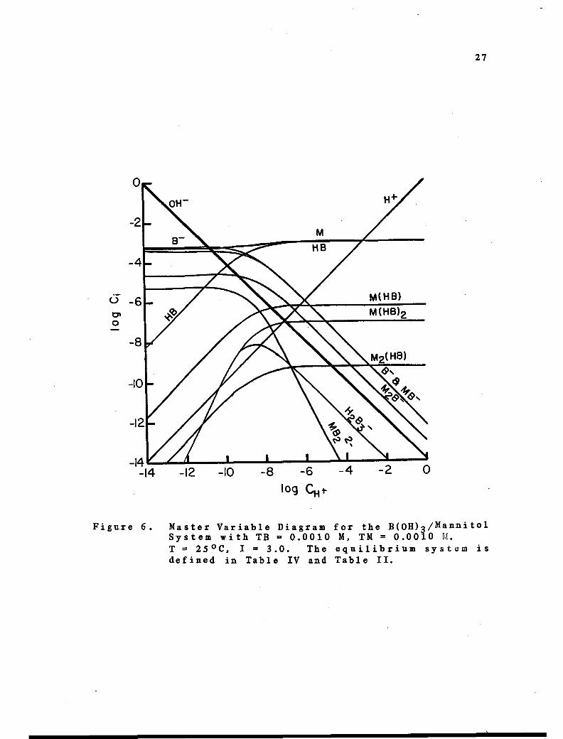
concentration are shown in Figures 6 8. Figure 9

illustrates the effect of the concentration of mannitol

upon the titration curve of 0.0010 M boric acid. A change

in the order of the predominant species occurs with

increases in the concentration of mannitol. With equal

concentrations of mannitol and borate the order of species

predominance in the basic domain is MB M2B and

the order of species predominance in the acidic domain

is HB > M(KB) > M(HB)2 > M2(HB). With a 10 fold excess of

mannitol the order of species predominance in the basic

domain changes to M2B MB > B, with no change in the

order of species predominance in the acidic domain. With

a 100 fold excess of mannitol the order of species

predominance changes to M2B > MB > and KB > M(HB)

M(HB) M (HB).2 As the concentration of mannitol

increases the clarity of the titration endpoint improves

and the inflection point shifts to lower log CH-1. values.

The figures illustrate that a factor of 100 excess

mannitol to total borate is necessary to accurately

determine low concentrations of boron.

aT = 298K, I = 3.0 M. For computations at I = 3.0 M the constants wereused as shown in the table. For computations at other ionic strengths,Equations 11 and 15 were used to correct the constants for the activitycoefficients, although it is recognized that use of Equation 11 isunjustified up to I = 3.0 M.

Table IV. ComponentsEquilibrium

Components:

and Species Considered in the B(OH)3/MannitolProblem. (1)

B(OH)4-, Mannitol (LH4), and 111-

Reaction Species Symbol logKa

"4 = LH4 M

B(OH)4- + LH4 - 2 1120 = LH2B(OH)2- MB- 2.99

B(OH)4- + 2L114 _4 1120 = I, -(LH2,2B -M2B 5.07

2B(011)4- + LH 4 - 4 H20 = L(B(OH)2)22- MB22- 4.41

2B(011)4- + LH4 + 2 H+ - 6 1120 = L(B(OH))2 M(HB)2 20

B(OH)4- + LH4 + le - 3 1120 = LH2B(OH) M(HB) 8.79

-B(O11)4 + 2LH4 + H - 4 H20 = (LH2)(LH3)B M 2 (HB) 8.77

2B(OH)4- + LH4 + le - 5 1120 = L(B(OH)2)(B(011))- MB(HB)- 7.2

-14-14 -12 -10 -8 -6

log Ctif

27

Figure 6. Master Variable Diagram for the B(OH) 1/MannitolSystem with TB = 0.0010 M, TM = 0.0010 H.T = 25°C, I = 3.0. The equilibrium system isdefined in Table IV and Table II.

-10

-12

OH-

-14-14 -12 -10 -8 -6

log CH+

28

Figure 7. Master Variable Diagram for the B(OH)3/MannitolSystem with TB = 0.0010 M, TM = 0.010 M.T = 25°C, I = 3.0. The equilibrium system isdefined in Table IV and Table II.

-14-14 -12 -10 -8 -6

I og CH+

29

Figure 8. Master Variable Diagram for the B(OH)3/MannitolSystem with TB = 0.0010 M, TM = 0.10 M.T = 25°C, I = 3.0. The equilibrium systemis defined in Table IV and Table II.

0.00

Fraction Titrated

Figure 9. Theoretical Titration of B(0103 in Mannitol.T = 25°C, I = 3.0. Fraction titratedrepresents moles of base added per mole of acid.Titrant was Li0H. The equilibrium system isdefined in Table IV and Table II.

[Mannitoi (M)

30

A 0.0B 0.001C 0.01D 0.1

31

Experimental

Several boric acid solutions (with and without

mannitol) have been titrated with Li011.

Apparatus

An Ingold glass pH ionselective electrode, model

5055-07, was employed as the indicating electrode (Figure

10). The glass membrane is 5 mm in diameter and designed

for use at temperatures between 00 70°C in the pH range

of 0 11. The special flat membrane surface allows for

use in small sample volumes, because less solution is

required for emersion of the membrane surface in a fiat

cell. Electrical resistance of the membrane is between

120 250 1152 at 25°C. The interior electrolyte, which

surrounds the Ag/AgC1 electrode, is a pH 7 buffer solution

with a defined potassium chloride concentration. An

internal shield extends the length of the electrode body

providing electrical shielding.

A GamRad double junction reference electrode model,

PEE 54473, was also employed (Figure 10). The upper

chamber is filled with a 4 M KC1 saturated AgC1 gel, and

the lower chamber is filled with a 4 M 1NO3 gel. Both

chambers were rinsed and refilled per recommended handling

instructions. The electrode has an Ag/AgC1 internal

Upper chamber4M KC1

hield

Internal referencesolution

Lower chamber4M

KNO3

Lead-off electrode

Glass membrane

Glass Electrode Double JunctionReference Electrode

Figure 10. Glass and Reference Electrodes.

32

33

reference element and the junctions are porous ceramic

cemented into a nylon base.

An Orion 701A digital pH/mV meter was used to measure

the potential between the electrode pair. The meter has

an input impedance of 1013

The performance of the H+ ionselective

electrode/double junction reference electrode pair was

tested before it was used for boron concentration

determinations. The results of these tests are given in

Appendix B. Good consistency was found between

calibrations with activity standards and with

concentration standards. Activity standards have been

used to calibrate the electrode pair in this study.

An automatic titration system, developed by C.M.

Seyfert (12), was used for all experimental titrations.

In the titration system the response of the electrode pair

is continually monitored to ensure that the change in the

potential with time, m, is less than a specified threshold

(m = 0.001 mV/s), before the next addition of titrant.

For a given set of time and potential data (tiEj), the

potential is expressed as a linear function of time

Ei = . + p (17)

The values of m and p are calculated to yield the best fit

to the experimental data by minimizing the sum of squares,

Yi, with respect to the parameters m and p

Y mti + p Ei

The automatic titration system was built with a

Metrohm 655 Dosimat to deliver titrant solution under the

control of a Rockwell AIM-65 microprocessor. The

millivolt response is read and stored by the

microcomputer and made available for print out and data

manipulation following the completion of the titration.

From previously determined ec ell and s values the pH at

each equilibrium point is calculated and included in the

final print out.

Realients

The chemicals used in this study were all reagent

grade and diluted with deionized water to the desired

concentration. (The deionized water was prepared by

passing house deionized water through a

catalog #2030 000 70, system consisting of an activated

charcoal bed and two mixed ion exchange beds). Solutions

were stored in polyethylene bottles to minimize

contamination from the borosilicate glass.

Procedure

The sample volume was pipetted into a water jacketted

34

(18)

35

beaker, thermostated to 25°C unless otherwise specified.

The solution was stirred at a constant rate and nitrogen

gas passed over the surface of the solution during

electrochemical measurement. The solution was titrated

with LiOH to an excess of 1.5 moles base per mole boric

acid. At the conclusion of each analysis the sample

solution was removed by suction and the cell rinsed

several times with deionized water.

Results and Discussion

Titrations of 0.0010 M, 0.010 M, 0.10 M, and 0.53 M

B(OH)3 were performed in the absence of mannitol. Figures

11-14 provide a comparison between the experimental and

computed titration curves. The log of the H+ activity is

plotted versus the fraction tit rated.

The experimental and theoretical titration curves are

contiguous at log all+ values less than 11. A slight

deviation is observed at log all+ values greater than or

equal to 11. This deviation is caused by the glass

electrode responding to other ions (i.e. Li+) in solution,

alkaline error. The deviation is less than 0.2 log all+

units in magnitude, which is consistent with expected

values. The correspondence of the experimental and

computed titration curves supports the equilibrium model

of the boric acid/borate system. The inflection point of

0

0

4

-8

10

12

Experimental Results

Equilibrium Model

36

0 0.50 1.00

FRACTION TITRATED

Figure 11. Titration of 0.53 M B(OH)3 with 1.00 M Li0H.T = 25°C. Fraction titrated represents molesof base added per mole of acid.

0

0


Equilibrium Model

0.50 1.00

FRACTION TITRATED

37

Figure 12. Titration of 0.10 M B(OH)3 with 1.00 M Li0H.T = 25°C. Fraction titrated represents molesof base added per mole of acid.

-4

10

12

1 i 1 t

0.50 1.00

FRACTION TITRATED

Figure 13. Titration of 0.010 M B(OH)3 with 0..100 M L10H.T = 25°C. Fraction titrated represents molesof base added per mole of acid.


Equilibrium Model

38

-4

4.

0

-10

-12

1


Equilibrium Model

39

0 0.50 LOU

FRACTION TITRATED

Figure 14. Titration of 0.0010 M B(OH)3 with 0.100 M

Li OH. T = 25°C. Fraction titratedrepresents moles of base Padded per mole ofacid.

40

the potentiometric titration curve is observed to occur at

the equivalence point of the titration (fraction titrated

equal to 1.0). It is important to note that the inflection

point of the potentiometric titration curve is difficult

to detect at the lower concentrations.

In a subsequent set of experiments the effect of

mannitol was investigated. From the equilibrium

calculations which included mannitol, the potential of the

electrode at the equivalence point was observed to be

dependent upon both the concentration of mannitol and

boric acid, Figure 9. Of further concern is the amount of

mannitol to be added per titration, the method of

titration endpoint detection, and the volume of sample

required per analysis. Titrations of the boric

acidimannitol solutions were performed using the

laboratory titration apparatus which had been programmed

to function as a typical commercial analyzer (13). Sample

volumes are initially determined by the operator based on

the expected boric acid concentration. Table V provides a

list of the analysis procedure, the breakdown of sample

concentration to sample volume, and the excess of mannitol

present. If, after completion of the titration, the boric

acid concentration falls outside of the predetermined

sample range, a second analysis is performed.

Titrations were performed on samples from within each

Range[B(OH)3](mg/L)

RangeIB(OH)3](M)

SampleVolume(mL)

ExcessMannitol

TB < 200 < 0.02 10 100a

200 < TB < 2000 < 0.20 2.5 10a

TB > 2000 >0.20 0.5 5b

a moles mannitol/moles maximum boric acidmoles mannitol/moles minimum boric acid

Analysis Procedures

Sample volume pipetted into the water jackettedbeaker.

10 mL deionized water is added to cover tip of pHelectrode.

If the solution is basic, 0.1 M HC1 is added to bringsolution to pH = 4.

2.5 mL of 0.5 M mannitol is added.

Solution is titrated with 0.100 M LiOH to pH = 8.5.

The microcomputer computes [B(OH)3]

Solution is removed by suction and the beaker rinsedseveral times with deionized water.

41

Table V. B(OH)3 Sample Breakdown and List of AnalysisProcedures.

4

6

-8

-10

-12

1.0

111,

MIR


Equilibrium Model

42

1


Figure 15. Titration of 0.50 M B(OH)3 in Mannitol.Titrant = 0.100 M Li0H, Volume of sample =0.50 mL, Volume of 0.5 M mannitol = 2.5 mL,Volume of 1120 = 10.0 mL, T = 25°C. Fractiontitrated represents moles of base added permole of acid.

-4

-6

8

-10

-12

NOW

M=Ilr

Ex perimental Results

Equilibrium Model

0.00 0.50 1.00

Fraction Titrated

Figure 16. Titration of 0.050 M B(011)3 in Mannitol.Titrant = 0.100 M Li0H, Volume of sample = 2.5mL, Volume of 0.5 M mannitol = 2.5 mL, Volumeof H20 = 10.0 mL, T = 25°C. Fraction titratedrepresents moles of base added per mole ofacid.

43

o WM,

4-

6

-8

12

=MP


Equilibrium Model


Figure 17. Titration of 0.0050 M B(011)3 in Mannitol.Titrant = 0.100 M L10H, Volume of sample =10.0 mL, Volume of 0.5 M mannitol = 2.5 mL,Volume of 1120 = 10.0 mL, T = 25°C. Fractiontitrated represents moles of base added permole of acid.

44

MEP

WIMP

0

10

45

concentration range. The experimental and computed

titration curves are illustrated in Figures 15-17. The

agreement between the curves is good. The good agreement

between the experimental and computed titration curves

is consistent with the stoichiometry and equilibria of the

boric acid/borate/mannitol system. The inflection point

of the potentiometric titration curve occurs at the

endpoint of the titration. Commercial titration

apparatuses titrate to a fixed endpoint of log an+ = 8.5.

Within this concentration range the inflection point of

the titration curve corresponds to log an+ = 8.5 0.02.

Table VI lists the fraction titrated determined at the

fixed log an+ = 8.5, and the percent relative error. The

titration to a fixed endpoint of log an+ = 8.5 was found

to be adequate for samples in the concentration range.

Conclusion

The concentrations and volumes of mannitol, titrant

and sample used were found to be suitable for determining

the concentration of boric acid in the range specified.

The addition of mannitol to sharpen the endpoint is

necessary below 0.10 M boric acid concentration. Mannitol

should be in excess relative to boric acid by

approximately a factor of ten below 0.10 M and a factor of

100 below 0.01 M boric acid.

[B(OH)3](M)

EndpointFractionTitrated

% RelativeError (%)a

46

Table VI. Fraction Titrated by Fixed Endpoint Detection.

where 1.00 is the fraction titrated at theequivalence point of the titration.

0.0050 1.023 2.3

0.050 1.005 0.5

0.50 0.996 -0.4

a % Relative Error =

fraction titrated log a11-8.5 -1.00x 100

1.00

The titration to a fixed endpoint of log

47

H+ = 8.5

was found to be adequate for samples in the range,

provided the electrodes are frequently standardized.

Evaluation of the pH electrode Appendix B, indicated

that the most likely interference will be a change in the

value of Ho', Equation 7. The interference will not alter

the equivalence point, but will alter the position of the

endpoint relative to the log aH+ of 8.5. It is therefore

recommended that the detection of the endpoint by a

derivative technique be employed.

48

SPECTROPHOTOMETRIC ANALYSIS

Introduction

A number of reagents have been employed for the

spectrophotometric determination of boron. Of them, the

most widely used reagents are curcumin (14, 15) and

carminic acid (16,17). The curcumin method involves

evaporation of an acidified boron/curcumin solution to

dryness, followed by dissolution of the residue into ethyl

alcohol. The carminic acid method requires use of

concentrated sulfuric acid and a lengthly equilibration

step. Both methods are unsuited for rapid analysis or

automated procedures.

Azomethine H, 4hydroxy-5[[(2hydroxyphenyl)

methylenelamino]-2,7napththalene disulphonic acid, has

been recommended by Korenman (18) as a reagent for

detecting boron qualitatively. In recent years several

researchers have demonstrated the use of azomethine H for

quantitative determination of boron concentration in steel

(19), raw water (5) and plant tissue (20) samples. The

procedure for its use is suitable for automation. Other

advantages for use of this reagent over use of other

spectrophotometric reagents include rapid analysis time,

simplicity of procedure, and small sample volumes.

Because of these advantages, azomethine H was selected for

49

use in the spectrophometric determination of boron

concentrations in this study.

The initial spectrophotometry studies focused on the

determination of the stability constants and molar

absorptivities for each species, and the rate constants

for each chemical reaction. Determination of these values

enabled calculation of the absorbance signal for any set

of boric acid concentration, azomethine H concentration,

and time conditions. In these studies the pH was

maintained at 5.0+0.2 with a buffer consisting of 0.147 M

acetic acid and 0.097 M ammonium acetate. The pH range

was selected because of previous studies by Capelle (19).

The buffer also maintains a constant ionic strength

environment, I 0.1 M. Within this pH range, at boric

acid concentrations below 0.1 M, the only significant

boron species present (determined in the previous section

of this thesis) is the monomeric boric acid species. A

temperature of 250C was selected to provide consistency

between the potentiometry and spectrophotometry studies.

The final spectrophotometry studies focused on the

design and testing of a flow system for the determination

of boron concentration via three analysis modes: stopped

flow, continuous flow, and flow injection. In stopped

flow analysis, the reagent and boron containing sample are

mixed and pumped into the spectrophotometer cell, flow is

stopped, and the formation of the complex is monitored as

50

time passes. Long reaction times are possible, allowing

for detection of lower boron concentrations. In

continuous flow analysis, the reagent and samples are

mixed and pass continuously through the spectrophotometer

cell, allowing for detection of more samples per hour. In

flow injection analysis, a plug of the sample is injected

into a flowing stream of the reagent. The sample reacts

with components of the carrier stream as it passes through

a mixing coil to the spectrophotometer cell. The

advantage of this mode is the small sample volumes

required.

Theory

In the following sections the theories applied in the

interpretation of the experimental data are discussed.

Spectrophotometry

Spectrophotometric methods are based upon the

measurement of decrease in radiant power of a beam of

light as it passes through an absorbing medium of known

dimension. When light of a small wavelength range passes

through a sample containing an absorbing species, the

radiant power of the beam is progressively decreased as

more of the energy is absorbed by molecules in solution.

The decrease in radiant power depends upon the

51

concentration of the absorber and the length of the path

traversed by the beam. The transmittance, T, of a

solution is defined as the ratio of the intensity of light

transmitted through the sample solution to the intensity

of light transmitted through a blank solution which does

not absorb light. The experimental absorbance is defined

as log T, and has been given the symbol abs. The Beer

Lambert law relates the absorbance to the concentration C

of the absorbing species and the optical path length b as

follows:

abs = ebC (19)

In this equation, E is the molar absorptivity, which is

dependent on wavelength. In spectrophotometric

determinations a calibration curve of abs versus C is

prepared from measurements of absorbance standards. This

curve is then used to determine C in a sample from the

measured absorbance for the sample.

The total absorbance of a solution at a given

wavelength is equal to the sum of the absorbances of the

individual species present. Thus, for a multicomponent

system

abstotal = E absi = e-bC- (20)

where the subscript i refers to all absorbing substances.

To obtain accurate results with spec trophotometry it is

52

desirable for the absorbance measured to be due

predominately to the analyte. Absorption due to other

species should be compensated by a blank measurement. The

absorbance signal should generally be in the range of 0.01

to 2.0 absorbance ,units (A.U.) for highest accuracy.

Below 0.01 A.U. or above 2.0 A.U. the precision decreases.

Although many substances absorb strongly in the

visible and near UV wavelength regions, many others do

not. Boric acid is one of those substances which do not

absorb. To determine the concentration of the

nonabsorbing boron, B(OH)3 is reacted with a reagent to

form an absorbing reaction product. It is important that

the reagent be selective for the species to be determined,

in order to prevent interference from other species in

solution. The reagent azomethine H has been selected for

use in this study because of the rapid analysis time and

the simplicity of its procedure. Azomethine H is readily

available as the condensation product of Hacid, 8amino-

1naphtho 1-3 , 6 disulphonic acid, and sal icaldehyde.

(Since only the H acid derivative was used in this study,

azomethine H will be referred to as azomethine). In

aqueous solution azomethine, Figure 18, is orange, whereas

Hacid and salicaldehyde are practically colorless. Boron

is complexed by the oxygen of the hydroxyl groups of the

azomethine molecule.

SO3H

Figure 18. Structure of Azomethine H.

N=CH

OHOH

53

Chemical Eguilibrium

As will be shown, an equilibrated solution of

azomethine, A, and boron, B, contains: free azomethine

and boron, an azomethine dimer, and 1:1 and 2:1 azomethine

boron complexes. The reactions for the formation of these

complexes can be expressed as

2A A2 (21)

A + B AB (22)

2A + B a2)3 (23)

where AB and A2B are the 1:1 and 2:1 complexes, and A2 is

the azomethine dimer. Whether some component of the

buffer was involved in the formation of the dimer was not

investigated.

Capelle (19) determined that the development of the

azomethine/boron complexes during the initial two hours is

fairly rapid, but 10 to 14 hours are necessary for the

system to equilibrate (T = 200 + 5°C, pH = 5.2). In this

section the theory and equations which characterize the

azomethine/boron system in equilibrium are presented, time

> 12 hours. Chemical kinetics which characterize the

system before equilibrium is reached are discussed in the

next section.

The absorption spectra for an equilibrted solution of

azomethine and boron and for the azomethine reagent are

54

= IABl_ (28)[A][13]

55

shown in Figure 19. The azomethine/boron complexes

exhibit a broad band centered at 412.5 nm. The azomethine

monomer and dimer exhibits a broad peak centered at 341

urn. Capelle (19) observed that the maximum equilibrium

absorbance signal from the complexes was obtained with

solutions buffered to pH 5.2, but that the absorbance

signal remained constant within the pH range 4.8 to 5.6.

The measured absorbance signal can be expressed as

abs = EA[A] 6A "23 EABEAB1 EA BEA2B1 + EB[B] (24)2 2

from Equation 20. All absorbance values have been

normalized to al cm path length. The absorbance due to

boric acid is insignificant within the wavelength range

studied. Materi-al balance equations for the total

azomethine and boron concentrations, TA and TB may be

written.

TA = [A] + 2[A2] + [AB] + 2[A2B] (25)

TB = [B] + [AB] + [A2B] (26)

The relationship between the concentration of the

complexes and reactants can be expressed as

KA = [A2] (27)

TiTI

I.00_

0.80

0.60

00.0

0.400co

.c3

0.20

0.00 A

300 350 400 450 500wavelength (rim)

Figure 19. Absorbance Spectra.Buffer: 0.147 M acetic acid/0.097 M ammoniumacetate, pH = 5. Azomethine H: 1.0 x 10-4 M.B(OH)3 = 0.1 M.Curve A: Buffer vs Buffer.Curve B: Azomethine H/Buffer vs Buffer.Curve C: B(OH)3/Azomethine H/Buffer vsBuffer.

56

57

where KA is the stability constant for the azomethine

dimer, K1 is the step wise stability constant for the AB

complex, and 02 is the cumulative stability"constant for

the A2B complex. Thus, to completely characterize the

absorbance of the system the values for the molar

absorptivities and stability constants must be determined.

Spectrophotometry is a widely used technique for the

study and determination of stability constants. However,

complications arise when fitting to absorbance

measurements because not only are the stability constants

to be determined but also the molar absorptivities for

each species. The computer program FITEQL (21) is used in

determining stability constants and molar absorptivities

for the boron/azomethine species. The program is general

in scope, having the capability to evaluate constants for

any species which can be expressed as the product of the

components. A set of components is defined such that

every species can be written as the product of a reaction

involving only the components. The representation of the

species in terms of the components is unique. Specific

parameters (e.g. stability constants and molar

absorptivities) in the chemical equilibrium problem are

adjusted to yield the optimal fit of the model to the

r32

(A2B](29)

58

experimental data. The optimization procedure involves

the iterative application of a linear approximation of the

chemical equilibrium equations and a linear least squares

fit. Whereas MICROQL (10) (described in the potentiometry

section) is used to determine total or free component

concentrations from given stability constants, FITEQL (21)

is used to determine stability constants from total and

free component concentrations.

Chemical Kinetics

The rate of a reaction is expressed as the change in

concentration of a reactant or product with time. An

equation that gives the reaction rate as a function of

concentration is referred to as a rate law. The rate law

for any chemical reaction must be determined

experimentally. A rate law which can be used to describe

the formation of the AB and A2B complexes has been

determined to be

&LAE. = kf1[A][8] kbi[AB] (30)dt

d[A2B] = kf2[A]2[B] kb2[A2B] (31)

dt

where kf, and kb, are the forward and backward rate

constants. The rate law can be expressed in terms of

only the complex concentrations and the total azomethine

59

and boron concentrations by combining Equations 25 and 26

with Equations 30 or 31.

Atal = kfl(TA-2[A2B]-EABD(TB-[A2B] -EABil-kbi[AB] (32)dt

d[A2B] = kf2(TA7-2[A2B](AB1)2(TB(A2B](AB]) kb2[A2B] (33)

dt

The concentration of the A2 species (Equation 25) is found

to be negligible. The reaction order with respect to the

concentration of one particular species, Ci, is defined as

order with respect to species i =

(salSi rate (34)slog Ci ) cj

where the reaction rate is evaluated under conditions such

that the concentrations of the other species, C.J'

constant. The definition of Equation 34 and the graph of

log rate versus log concentration are used in practice as

a means of formulating an alegebraic relation between

rection rate and species concentration. A rate law

involving reaction orders greater than I cannot always be

solved directly. In this case the solution to the rate

equation can be approximated by numerical integration,

whereby the concentrations of the species are repetitively

determined for small changes in time. This numerical

integration has been performed according to the

trapezoidal rule.

are

60

Insight into the problems of kinetic analysis can be

gained when certain simplifying assumptions are made with

regards to Equation 30 and 31.

Case I. The reaction does not approach equilibriumduring the period of time under considerationand the magnitude of the back reaction isnegligible compared to that of the forwardreactions:

4dAR1 = kn. (TA-2[A213]-(ABD(TB-[A2B]-[AB]) (35)dt

d [A2 = kf2 (TA-2[A2131 [AB] )2(TBIA2B] [AB]) (36)

dt

Case II. The assumption in Case I holds. Also theconcentration of either complex formed isnegligible compared to the total concentrationof boron or azomethine thus [B] TB and [A]TA are effectively constant:

d[AB] = kn. TA TB (37)

dt

d[A2B] kf2 TA2TE (38)

dt

These cases can be applied to a reaction whether it is the

only reaction or one of many occurring in solution. The

assumptions which apply, however, must be specified for

each case.

Ex2erimental

The experimental section has been divided into two

61

parts. In the first section the apparatuses, reagents and

procedures used in determining the equilibrium and kinetic

constants are described. In the second section the design

and operation of a flow system for the determination of

boron concentration are described.

Aknaratus

A Cary 118C UVvis spectrophotometer with 1 and 10 cm

glass cells and an ISCO V4 variable detector with 0.5 cm

glass flow cell were used for all spectrophotometric

measurements. All absorbance values have been normalized

to a 1 cm path length.

Res/ents

The chemicals used in the study were all reagent

grade. Deionized water was used for dilution to the

desired concentration. Solutions were stored in

polyethylene bottles to minimize possible contamination

from borosilicate glass. Aqueous solutions of the

azomethine reagent are stable for 12 hours. After this

period, the solution shows signs of decomposition,

probably due to oxidation and/or hydrolysis. Ascorbic

acid (2.2 grams per gram of azomethine) is added as a

stabilizer. The ascorbic acid does not absorb within the

wavelength range of interest. Aqueous solutions of

62

the reagent and ascorbic acid are stable for 24 hours.

The buffer consisted of 0.147 M acetic acid and 0.097 M

ammonium acetate.

Procedure

Solutions were prepared by first mixing the boric

acid and buffer in a volumetric flask, followed by

addition of the azomethine reagent, and dilution with

deionized water to volume. Solutions were kept in a

constant temperature bath except during absorbance

measurements. The concentrations of azomethine and boric

acid for four sets of experiments are given in Table VII.

The change in absorbance versus time was recorded

continuously for 10 minutes. Additional absorbance

measurements were made at two hour intervals for 25 hours.

If the absorbance of a solution exceeded 2 A.U., the

solution was diluted in a 1:4 ratio with the buffer

solution. Dilution was performed in the absorbance cell.

Disassociation of the complexes upon dilution was not

detected within the time of measurement.

Results and Discussion

Eguilibrium

Before an attempt is made to discuss the interaction

of azomethine with boron, it is useful to consider the

Table VII. Experimental Concentations.

1.00 x 10-5 - 2.5 x 10-3 0.00

Experiment TA (M) TB (M)

II 5.00 x 10-4, 1.00 x 10-3, 5.00 x 10-4, 1.00 x

1.00 x 10-3 2.00 x 10-3

III 1.00, 2.0, 5.0 x 10 x 10-3

-41.00, 2.0, 5.0 x 10

1.00, 2.0, 5.0 x 10-3

IV 1.00 x 10-4 1.00, 5.00 x 10-4

1.00, 5.00 x 10-3

1.00, 5.00 x 10-2

1.00, x 10-1

64

aqueous chemistry of azomethine alone. In Experiment I

the absorbance signal of the azomethine solution remained

constant during the time of measurement. A linear

relationship between absorbance and the total azomethine

concentration was observed with solutions less

concentrated than 2.0 x 10-4 M. Figure 20 illustrates

this relationship at a wavelength, X, of 341 nm, the

absorption maximum of the azomethine reagent. With

sample concentrations greater than 2.0 x 10-4 M a

quadratic relationship was observed between absorbance

versus total azomethine concentrations. Figure 21

illustrates this relationship at X = 412.5 nm. Because

the wavelength of maximum absorbance for the

boron/azomethine complexes is known to be 412.5 nm, the

data collected at this wavelength have been interpreted.

The quadratic relationship provides evidence for the

existence of more than a simple azomethine species. The

data are interpreted in terms of two species: an

azomethine monomer, A and an azomethine dimer, A2.

The mass action equation for the formation of the

dimer, the mass balance equation for azomethine, and

Beer's law can be combined to form a relationship between

the absorbance and EA, EA2 and KA. From this relationship

and the experimental data, values for the constants are

determined.

2.00

0.000.0E+00 1..0E-04

[TA] CM)2.0E-04

Figure 20. UV Absorbance of Azomethine H.Wavelength = 341 nm, Acetate Buffer = 0.244 M, T = 25° C.Data from Experiment I.

%moo

0.10

0.75

0.50

izt 0.25

0.000.0

Figure 21. Visible Absorbance of Azomethine H.Wavelength = 412.5 nm, Acetate Buffer = 0.244 M, T = 25°C.Data from Experiment I.

2.51.0 1.5

11.4 (rnm)0.5 2.0

67

The material balance equation for total azomethine, TA,

in the absence of boron can be expressed as

TA = [A] + 2[A2] (39)

Equation 27 and 39 can be solved for (Al and (A2]

[A] = 1 + (1 + 8 KATA)1/2 (40)

4KA

[A2] = 1 + 4KATA (1 + 8 K TA)1/2 (41)

8KA

If the product 8KATA is small compared to 1, the square

root term can be approximated by polynomial expansion

161

The appropriate roots from the quadratic equation have

been chosen as not to violate the material balance

equation. The absorbance is expressed as

= CA[A] EA 2[A2](42)

Substituting Equations 40 and 41 into Equation 42 yields

= EA 4ICATA + (CA 2cA)(1 (1 + 8KATA)1/2) (43)2 2

(1+8KATA)1/2 = 1 + 4KATA 8(KATA)2 + 32(KATA)3 + ... (44)

68

If KA and TA are small (so that little of the dimer is

formed) only the first two terms need to be included in

the approximation.

(1 + 8KATA)1/2 q, 1 + 4KATA (45)

and the absorbance is expressed as

a b s E ATA (46)

The experimental data were observed to fit Equation 46 when

the total azomethine concentration was less than 2.0 x

10-4 M. As TA is increased, inclusion of the third term

in the square root approximation becomes necessary

(1 + 8KATA)1/2 1, 1 + 4KATA 8(KATA)2 (47)

and the absorbance is expressed as

AhA EATA + (EA 2 EA)KATA2 (48)2

The experimental data were observed to fit Equation 48

when the total azomethine concentration was greater than 2

x 10-4 M. Inclusion of additional polynomial terms in the

square root approximation was not required

concentrations less than 0.01 M TA.

Values for EA and the product (EA 2EA )KA have2

been determined from the first and second order

69

coefficients of a leastsquares fit to the polynomial in

Equation 48. If a second linear region had been observed

at higher TA concentrations, where conversion of the

monomer to the dimer was essentially complete, values of

CA and KA could have been resolved from the product2

CA KA This condition, however, was never observed. For2

convenience, KA has been assigned the value of 1, which is

consistent with the experimental observation that a

negligible fraction of the azomethine is converted to the

dimer over the concentration range studied. The values

determined for CA, EA , and KA are presented in Table2

VIII. The experimental absorbances along with the

calculated absorbances have been graphed in Figure 22.

Excellent agreement over the entire concentration is seen,

supporting the validity of the model.

With an understanding of the azomethine equilibria it

is possible to characterize the azomethine/boron

equilibria. In Experiments II, III, and IV equilibrium

was reached after 50 kilosecon.ds. A quadratic

relationship was observed between absorbance and the total

azomethine concentrations for a given constant total boron

concentration. The relationship between the absorbance

versus total azomethine suggests the presence of an A2B

species. There was also evidence for an AB species was in

the equilibrium speciation. Equation 25-29 completely

define the azomethine/boron system.

Table VIII. Azomethine H Equilibrium Constants.

Monomer A 14

Dimer A2 KA = 1

70

Stability MolarSpecies Symbol Constant Absorbitivity

(A.U. cm

0.10

0.05

tr

co

0.000-0E-4-00

ON,

10E-04 2.0E-03[TA] (M)

3-0E-03

Figure 22. Absorbance of Azomethine H.Wavelength = 412.5 um, Acetate Buffer = 0.244 M, T = 25°C.* Experimental Absorbances, Experiment I.--- Calculated Absorbances, Equation 48 and Table VIII.

sy2(m)

SOS = 1E2----

(m)

aTA

y )2

aTB

2

sTA (in)

in

in

2

sTB (m)

72

The equilibrium constant and molar absorptivity values for

the azomethine monomer and diner have been previously

discussed. Values for the stability constants and molar

absorptivity values for the boron/azomethine complexes

have been determined using FITEQL (21). In the program

the parameter adjustment procedure is based on minimizing

the sum of squares, SOS, over all the experimental data

points, in

(49)

where Y(m) is the difference between the calculated and

the experimental absorbances. The calculated absorbance

is determined from Equation 24, where the species

concentrations have been determined using Equations 25

29 with the current values for the adjustable parameters.

The propagation of experimental error, 5Y(m) is calculated

from

(50)

(Y-8ab

2

tabs (m)in

73

where sTA, sTB, and sabs are the estimated errors in the

experimental data. It is assumed that the errors in each

term are independent (noncorrelated) such that the sum

of the cross terms is equal to zero. The derivatives that

appear in the error propagation equation are calculated

from the chemical equilibrium equations. The estimated

errors in the experimental data have been calculated from

the following formulae

sTA = 1 x 10-6 M + 0.01 TA

sTB = 1 x 10-6 M + 0.01 TB

sabs = 4 x 10-3 A.B. + 0.01 abs

where the first number in the formula is an estimation of

the absolute error and the second is an estimation of the

relative error in the experimental measurements.

Values for the stability constants and molar

absorptivities for five equilibrium species have been

calculated and are listed in Table IX. The experimental

and calculated equilibrium absorbances have been graphed

in Figure 23. The absorbances greater than 2.0 A.B. are

effective absorbances, abseff, determined from

measurements of diluted samples. A comparison of the

Table IX. Azomethine R/B(OH)3 Equilibrium Constants.

S.D.a ofMolar Molar

Absorptivity Absorptivity(AU. cm-114-1) (A.B. cm-1 M-1)

Azomethine R A -- __ 14monomer

Azomethine H A2 KA = 1 -- 9.7 x 103 --

B(OH)3 B -- 0.00

1:1 complex AB K1 = 7.9 13 6.7 x 103 .+ 1 0 x 104

2:1 complex A2B $2 = 1.2 x 105 + 7.5 x 103 2.0 x 10 + 9.8 x 1024

a Number of data points = 18.Data from Experiments II and III. Constants for A and A2 determinedpreviously using data from Experiment I.

S.D.a ofStability Stability

Species Symbol Constant Constant

0.0xla[TA] (m)

75

Figure 23. Equilibrium Absorbance.Acetate buffer = 0.244 M, T = 25°C. Solidline represents calculated absorbance.For absexp > 2.0 A.U., abseff = absexp x 5.Data from Experiment II.

76

experimental and calculated absorbances is presented in

Table X. The relative error in the difference between the

calculated and experimental absorbances is about 3%. When

equilibrium constants and molar absorptivities are

determined simultaneously from spectrophotometric data,

there is a covariability in the values determined. Thus

while the constants determined here represent the data

very well, they are not necessarily the only combinations

of E and K which could represent the data. Some of the

problems associated with this affect have been discussed

by Johnansson (22). But, regardless of its lack of

uniqueness, the equilibrium model is an excellent

representation of the experimental data over the

concentration range considered.

From Equations 25-29 a comparison of the absorbance

contribution from each species is possible, Figure 24.

The effective absorbance versus total azomethine has been

plotted for total boron concentration 2 x 10-3 M. The A2B

species is the predominate absorbing species. The

absorbance contributions from the azomethine monomer and

dimer are comparable. The concentration of the monomer is

large but its molar absorptivity is small, while the

concentration of the dimer is small but its molar

absorptivity is large. As the concentration of total

azomethine is increased, formation of the A2B species over

Table X. Comparison of Experimental and CalculatedEquilibrium Absorbance s.

a relative difference = absc" abscal

abs

TA(M)

TB(M)

abse"(A.U.)

abscal absc" abs cal(A.B.)

relativedifferencea(%)

2 x 10-3 2 x 10-3 6.822 6.765 0.057 0.842 x 1 x 10-3 4.266 4.427 0.20 4.72 x 10-3 5 'lc 10-4 2.552 2.634 0.082 3.2

1 x 10-3 2 x 10-3 2.444 2.498 0.054 2.11 x 10-3 1 x 10-3 1.590 1,565 0.025 1.61 x 10-3 5 x 10-4 0.937 0.909 0.028 3.0

5 x 10-4 2 x 10-3 0.810 0.830 0.020 2.45 x 1 x 10-3 0.491 0.489 0.002 0.415 x 10-4 5 x 10-4 0.280 0.272 0.008 2.9

8.00

6.00

/-s

1 4.00

2.00

0.00

0.100

0.050

/A, 71.

Figure 24. Absorbance of Individual Species.TB = 2.0 x 10-3 M, Acetate Buffer = 0.244 M,T = 25°C.--- Total abs -- A abs---A2B abs _._ A2 abs

AB abs

-k1:3

78

79

the AB species is favored. Because the A2B species

complexes two azomethine molecules, there is less and less

of an increase in the free azomethine concentration per

increase in the total azomethine concentration. This

effect is observed in the bending over of the AB and A

absorbance curves, and a bending up of the A2B and A2

absorbance curves.

Kinetics

The course of the reactions can be divided into two

periods the initial period (t < 1000 s) in which the

concentration of free azomethine and free boric acid

remain approximately constant, and the long term (1000 s <

t < 60 ks) in which the concentration of the complexes

becomes significant.

In Experiments II, III, and IV the absorbance during

the initial 600 s was recorded as a function of time.

From these recordings the initial rate, d(abs/b)/dt, has

been calculated. During the initial 600 s the

concentration of both complexes is negligible compared to

the total boron and azomethine concentrations, and

therefore Case II has been used to interpret the data.

The plot of log rate versus log TA at constant TB defined

a straight line with a slope of 2, and the plot of log

rate versus log TB at constant TA defined a straight line

d(abs)AB/b) =

dt

kfiTATB (53)

The value for the forward rate constant has been

80

with a slope of 1. These plots suggest that the initial

reaction is first order with respect to TB and second

order with respect to TA.

A graph of the initial rate versus TA2TB is shown in

Figure 25. The solid line represents the function

= mTA2TB + c (51)dt

which is a linear approximation describing the rate as a

function of the product TA2TB. The first term has been

interpreted in terms of the formation of the A 2B complex.

The value of the intercept c is small and corresponds to

the contribution from the AB complex.

The initial rate law for the formation of the A2B

complex can be expressed as

d(abs A B/b) = E2kf2 TA2TB (52)2

dt

The value of the forward rate constant has been determined

from the slope of the initial rate versus TA2TB. The

initial rate law for the formation of the AB complex can

be expressed as

B.0E-04

6.0E-04

4.0E-04

2.0E-04

0.0E4-000.0E-4-00 2.0E-09 4.0E-09 6.0E-09 8.0E-09

TA2TB (M)3

Figure 25. Initial Rate Analysis. Acetate Buffer = 0.244 M, T = 25°C,Rate = 93079 TA2TB + 9.6 x 10-6.Data from Experiments II, III, and IV.

82

determined by optimizing the fit of the calculated rates

given by Equations 52 and 53 to the observed rate.

A graph of absorbance versus time for TA = 5 x 10-4

M, TB = 2 x 10-3 M during the initial 1000s is shown in

Figure 26. These experimenal conditions favor the

formation of the AB complex. The solid circles represent

the experimental absorbance signal. The dashed line

represents the absorbance contribution from the formation

of the A2E complex, and the dotted line represents the

absorbance contribution from the formation of the AB

complex. The solid line represents the total calculated

absorbance as the sum of the absorbance from the A2B and

AB complexes. It is seen that even for experimental

conditions favoring the formation of the AB species, the

contribution of the AB species to the total absorbance is

small and becomes less with time.

The above discussion assumes that the concentration

of free azomethine and free boric acid remain

approximately constant, and that the back reactions are

insignificant (Case II). However, when considering the

entire approach to equilibrium, the concentration of the

complexes becomes significant in the material balance

equations and the back reactions must be considered. To

be consistent over the entire course of the reaction, from

initial to equilibrium conditions, it is necessary to

express the reaction rate as

c.)

2002. /I

C:C

0.06

0.04e/

0.0Qu.00 0.50

Time (ks)

1.00

83

Figure 26. Initial Kinetics of Individual Reactions.TA = 5.0 x 10-4 M, TB = 2.0 x 10-3 M, AcetateBuffer = 0.244 M, T = 25°C.

absexp A2B abs + A2 abs

--- Total abs AB abs

OOOOO

.w .m.im empla

......

dilbsLki = EAd[A] "I' EA dIA2] EABd[AB] + e ArA Bl (54)A B---2dt 2 2

dt dt dt dt

where the rate equations for the AB and A2B complexes are

expressed in Equations 30 and 31. The relative values of

the forward and backward rate constants are fixed by the

relationsfi 2 k f 2 / kb2 and IC

kfl/kbi. Values for the backward rate constants have

been determined from the equilibrium stability constants.

Values for both sets of rate constants are listed in Table

XI.

The concentration of each complex during the approach

to equilibrium has been approximated by simultaneous

numerical integration of Equations 30 and 31 subject to

Equations 25 and 26 at 10 second intervals (constants from

Tables IX and XI). For each 10 s interval the rate

integral is estimated by the area of a trapezoid. The sum

of each of these areas results in an approximation of the

total absorbance for a time t.

The experimental and computed absorbances have

been plotted versus time. Figures 27-29 illustrate the

absorbance development during the initial 1000s and

Figures 30-32 illustrate the absorbance development during

the entire approach to equilibrium. The experimental

absorbances greater than 2.0 A.B. are effective

absorbances, abs eff, determined from measurements of

solutions which have been diluted. In each figure TA is

84

constant. The solid line represents the calculated

Table XI. Kinetic Rate Constants.

SpeciesStabilityConstant

Forward Rate Backward RateConstant Constant

AB 7.9 1.8 x 10-3 s-1M-1 2.3 x 10-4s-1

A2B 1.2 x 105 4.7 s-1M-2 4.0 x 10-5s-1

0.600

0.600CIE

0.400ala

0.200-0

0.0000.0 200.0 400..0 600.0

Time (s)

Figure 27. Initial Kinetics of Reaction: TA = 5.0 x 10-4 M.Acetate Buffer = 0.244 M, T = 25°C.Solid line represents calculated absorbance.* TB = 2.0 x 10-3 M, + TB = 1.0 x 10-3M, x TB = 4.0 x 10-4M.

800.0 1000.0

Q ) 0.40000la0

0.200

400.0

Time (s)

Figure 28. Initial Kinetics of Reaction: TA = 1.0 x 10-3 M.Acetate Buffer = 0.244 M, T = 25°C.Solid line represents calculated absorbance.* TB = 2.0 x 10-3 M, + TB = 1.0 x 10 M, x TB = 5.0 x 10-4 M.

co

0.800

0.6000

a) 0.400C

_o

0.200.C1

0.0000.0 200.0 400.0

Time (s)

Figure 29. Initial Kinetics of Reactions: TA = 2.0 x 10-3 M.Acetate Buffer = 0.244 M, T = 25°C.Solid line represents calculated absorbance.* TB = 2.0 x 10-3 M, + TB = 1.0 x 10-3 M, x TB = 5.0 x 10-4 M. oo

600.0 800.0 1000.0

1.00

0-75

0-50

0.00-25

20-00 40.00 60.00

Time (ks)

Figure 30. Kinetics of Reaction: TA = 5.0 x 10-4 M.Acetate Buffer = 0.244 M, T = 25°C.Solid line repre§ents calculated absogbance.* TB = 2.0 x 10.° M, + TB = 1.0 x 10 M, x TB = 5.0 x 10-4 M.

3.00

2..00

Figure 31. Kinetics of Reaction: TA = 1.0 x 10-3 M.

Acetate buffer = 0.244 M, T = 25°C.Solid line represents calculated absorbance.* TB = 2.0 x 10-3 M, + TB = 1.0 x 10-3 M, x TB = 5.0 x 10-4 M.For absexp > 2.0 A.U., abs eff = abs x 5.

20.00 40.00

Time (ks)60.00

20.00 40.00 60.00

Time (ks)

Figure 32. Kinetics of Reaction: TA = 2.0 x 10-3 M.Acetate Buffer = 0.244 M, T = 25°C.Solid line represents calculated absorbance

Lc)* TB = 2.0 x 10-3 M, + TB = 1.0 x 10-3 M, x TB = 5.0 x 10-4 M.For absexp > 2.0 A.U.p abseff = absexp x 5.

92

absorbance at time t by the integration described in the

preceding paragraph. The * +, and x represent the

experimental absorbances for TB = 2 x 10 M, 1 x lo-3 m,

and 5 x 10-4 M, respectively.

The absorbance development is linear with respect

to time during the initial 1000s. Figures 27-29 have been

graphed on the same absorbance axis scales to illustrate

that the increase in the rate is greater per increase in

TA as compared to the same increase in TB. Higher

concentrations of TA will enable determination of lower

boron concentrations for a fixed measurement time because

a greater absorbance signal is obtained.

Figures 30-32 have been graphed on different

absorbance axis scales to illustrate that the absorbance

development curves follow the same general shape. The

equilibrium absorbances have been previously discussed and

are graphed in Figure 23. The length of time to

equilibrate is similar for all solutions within this

concentration range.

It is of interest to show the contribution of each

complex to the total absorbance. A graph of the computed

concentrations of each species during the approach to

equilibrium is provided in Figure 33, TA = 5 x 10-4 M and

TB = 2 x 10-3 M. These experimental conditions are

favorable for the formation of the AB complex. The

absorbance contribution for each species is provided in

Figure 34. The shape of the total absorbance versus time

20.00 40.00 60.00TIME (kS)

Figure 33. Kinetics of Individual Reactions. Concentration vs. Time.TA = 5.0 x 10-4 M, TB = 2.0 x 10-3 M,Acetate Buffer = 0.244 M, T = 25°C.

0.00

Total AbsorbanceA2BABA&A2

Figure 34. Kinetics of Individual Reactions. Absorbance vs Time.TA = 5.0 x 10-4 M, TB = 2.0 x 10-3 M,Acetate Buffer = 0.244 M, T = 25°C.

60.00

0.1300

lii

0.600

Li

0.400ED

Er

00.200

0.000 40.00(kS)

20.00TIME

95

curve is due primarily to the absorbance of the A2B

complex. The AB species has been shown to be important

during the initial 1 ks (Figure 20.

The rate equations and corresponding rate constants

have been empirically determined. Thus while the

equations and constants presented here represent the data

very well, they are not necessarily the only

interpretation which could represent the data. But,

regardless of its lack of uniqueness, the kinetic model is

an excellent representation of the experimental data over

the concentration range considered.

Predictions of the total absorbance and species

concentration during the system's approach to equilibrium

are possible. These predictions are useful in determining

optimal experimental parameters for the analysis of boron

within a specified concentration range. This application

is demonstrated in the flow system optimization section

of this thesis.

122lication

A flow system has been designed f or the

determination of boron concentration via three different

kinetic analysis modes: stopped flow, continuous flow,

and flow injection. In stopped flow analysis, the

reagents and analyte are mixed and pumped into the flow

through detector, flow is stopped and the formation of the

96

complex is monitored as time passes. Long reaction times

are possible, allowing for more complete development of

the colored complex and detection of lower concentrations.

Because the absorbance of the blank does not vary

significantly with time, although the reagent is being

constantly consumed, only a single blank measurement is

no

In continuous flow analysis, the reagents and analyte

are mixed and flow continuously through a delay loop to

the detector. The short reaction times in continuous flow

analyses increase sample throughput, but decrease

sensitivity. However, with high concentrations of boric

acid the sensitivity is sufficient.

Flow injection analysis is based on injection of a

liquid sample into a moving carrier stream of reagent.

The injected sample forms a zone that disperses on its way

to the detector. In this zone the sample reacts with

components of the carrier stream forming a colored species

to be sensed in the flow through detector. A typical

recording has the form of a sharp peak, the height of

which is related to the concentration of the analyte. The

advantage of this mode is the extremely small sample

volumes (100 PL) required. The disadvantage is the low

sensitivity due to the small sample size and short

97

reaction time. However, the low sensitivity is not a

problem with high concentrations of boric acid.

With kinetic methods the rate of formation of the

colored complexes is of importance rather than the

equilibrium absorbance signal. Kinetic methods have been

defined and classified by Pardue (23). The techniques

presented here are fixed time methods, where the

absorbance signal is recorded at.a fixed measurement time.

There are several advantages in using kinetic methods

for analytical purposes as opposed to equilibrium methods.

The kinetic method is faster since measurements are made

before equilibrium is reached. The dynamic range of

kinetic method can be extended by adjusting the time of

measurement. Kinetic methods have certain limitations

since they involve the detection of a quantity related to

the rate of reaction. These limitations include the need

for strict control of reaction conditions (e.g. pH,

temperature, time).

Flow System DesiAn

A diagram of the flow system is provided in Figure

35. For continuous and stopped flow analysis, the 2-way

valve is in position A. The 3-channel pump allows

different concentrations of the azomethine reagent and

acetate buffer to be prepared. The standards or samples

THREE

CHANNEL

PUMP

III ACETATE BUFFER

AZOMETHINE

II2

SAMPLES

STANDARDS

6-WAYVALVE

SINGLE

CHANNEL

PUMP

CONSTANT

TEMPERATURE

BATII

2-WAYVALVE

INJECTION

VALVE

1

I I

WASTE

CONSTANT

TEMPERATURE

BATH

RECORDER

I II I

COLORIMETRIC

DETECTOR

I I

I I

I I

I I

A/D

AIM-65

WASTE

Figure 35. Flow System for Spectrophotometric Analysis. Pumps, valves,and data acquisition controlled by microprocessor.

99

are selected with the 6way valve and pumped to a tee by

the single channel pump. At the tee the reagent/buffer

solution and sample solution merge, and flow through a

mixing coil submerged in a constant temperature bath, and

on to the absorbance flow cell. After measurement the

solution flows into a waste container. Continuous

measurements are made while the solution is passing

through the flow cell. In stopped flow analysis the flow

is stopped while the solution is present in the flow cell

and the progress of the reaction is monitored for the

portion of time of interest. The flow is stopped by

halting both pumps.

For flow injection measurements the 2way valve is in

position B. The reagent/buffer solution is prepared as

described previously. The selected sample is pumped to

the injection loop by the single channel pump with the

excess sample solution flowing into a waste container.

The sample is introduced as a plug into the reagent/buffer

main stream. The combined flow goes through the mixing

coil, absorbance flow cell, and into the waste container.

The flow injection measurements are made when the plug

travels through the flow cell and absorbance peak heights

are measured.

Components for the system which were adaptable to

microcomputer control were selected for use. The

injection loops and valves were equipped with pneumatic

100

activators to allow computer controlled switching. The

major components of the system are each described in

greater detail in the following paragraphs. Table XII

contains a list of the components and their sources.

Components

The 3channel pump is a microprocessor controlled

solvent delivery system, designed for pumping up to three

solvents in various compositions at precisely controlled

flow rates and pressures. External remote control of the

pump unit is made with a +5 volt pulse to either the run

or stop hook ups. The control unit monitors the flow rate

feedback loop to minimize flow variations. Flow rates

from 0.1 to 9.9 mL/min are possible with 3% accuracy. The

pump usually operates at 2.0 mL/min combined flow. The

buffer comprises 50% of the flow volume with the remaining

50% a dilution of a 0.015 M azomethine solution.

The automatic sample injector is a 6 port rotary

injector. The advantage of this injector is that a wide

range of injection loop volumes may be installed. In the

load position solvent bypasses the injection loop which

is being filled with sample. Solvent flows through the

sample loop in the inject position. With complete loop

loading volumetric precisions of 0.05% are possible. The

absorbance flow cell used in the system was designed for

Table XII. Flow System Components.

Component Source Comments

3channel pump Spectrophysics Model 8700

Automatic Sample Injector Rheodyne Model 7126, pneumatic actuatorModel 7163, solenoid valve

positive sensing switch

Constant Temperature Bath HAAKE 3 gallon, circulating pumpmaintains T + 0.1°C

2way valve Rheodyne Model 5301, slider valveModel 5300, pneumatic actuator

6way valve Rheodyne Model 5011

Singlechannel pump Fluid Metering, Inc. Model RHSY1CKC

Flow Cell ISCO 5 mm path length cat. #68-0080-045

Colorimeter ISCO Model V4 variable wavelengthdetector

Recorder Linear Instruments Model 585, duel channel

A/D Analog Devices #574 for 8 bit analog todigital interface

AIM-65 Forthought Products

102

absorbance detection in high pressure liquid

chromatography. The flow cell cross section is seen in

Figure 36. The 0.5 cm light path contains 3.5 gL of

illuminated volume. The flow path follows a zshape which

provides a longer path length than a straight through flow

configuration. The flow is away from the light source of

the V4 variable wavelength absorbance detector.

The V4 is a variable wavelength photometric detector.

The optical system includes a diffraction grating

monochromator. A tungsten lamp is the light source in the

350-750 nm range, and a deuterium lamp is the light

source in the 190-350 nm range. Wavelength accuracy is +

1 nm with + 0.5 nm repeatability. The spectral bandpass

is 5 nm. The recorder output is connected to an external

strip chart recorder and an analog to digital converter,

AID.

Teflon tubing was used for all flow paths. The

mixing coil is comprised of 15 loops, each 13 cm in

diameter.

Computer control was emphasized in the design and

construction of the flow system so that operation of the

system could be controlled by software. A Rockwell AIM-65

microcomputer has been programmed to control the entire

system.

For convenience, the main program was written to

accomplish these tasks in BASIC, while assembly language

LIGHT>

OUT

IN

ILLUMINATEDVOLUME(3.5 L)

LEAD CONNECTOR

103

Figure 36. Absorbance Flow Cell. Path length = 0.50 cm.

104

subroutines are utilized for data collection and control

of the system components. A single program is used for

all three modes. Absorbance data is stored in data files

which are read by a second program for calibration and

concentration calculations. A complete listing of both

programs is provided in Appendix C.

Optimization of Flow System Parameters

The parameters of this system have been optimized

with regards to the range of boron concentrations expected

in nuclear reactor coolant water and the signal limitation

of the colorimeter (0.01 1.00 A.U.) per absorbance range

scale setting.

The parameters considered are

flow rates

timing

total azomethine H concentration

stopped flow development time

injected sample volume

Adjustments of the flow rate of each pump were made

to obtain the desired mixing ratio of the

sample:buffer:reagent. A compromise between rapid rates

for rinse out of the flow cell and complete filling of the

sample lines and slow rates for maximum delay periods was

necessary. A 1:1:1 ratio of sample:buffer:reagent was

desired. The flow rate of the 3channel pump was set at 2

mL/min and the single channel pump was set at 1 mL/min.

105

At these flow rates 350 seconds were required to rinse out

the single channel pump and the flow cell, and to fill the

sample line. The delay time from sample/reagent mixing to

absorbance detection was 30 seconds.

The optimum value of total azomethine H concentration

can be calculated from the estimated concentration of

boron, the analysis time, and the integrated form of the

initial rate equation, Equation 51

abs = (mTA2TB + c)t (55)

In this equation m is the slope of the initial rate versus

TA2TB, and c the absorbance intercept. The maximum

concentration of B(OH)3 is approximately 0.9 M (solubility

of B(OH)3 at 25°C) (11), which will be 0.3 M in the flow

cell after online dilution. If this sample is to be

analyzed via continuous flow analysis (t 30s) and have

an absorbance signal of 1 A.U., the azomethine H

concentration in the flow cell must be 1.5 mM. The 3

channel pump reservoir has been filled with an 0.015 M

azomethine and diluted online to obtain a 1.58 mM reagent

solution.

The stopped flow development time was also determined

from Equation 55 for an absorbance of 0.01 with a 5 x 10-4

M boric acid solution. A delay time of 500 seconds would

provide enough time for color development and make the

106

total analysis time less than 20 minutes per sample.

The sample loop volume for flow injection analysis

was selected as to obtain the tallest peak possible yet

still have complete mixing of the sample plug with the

reagent flow. A 100 gL loop was best able to meet both

criteria.

The following list summarizes the parameters for the

flow system

Flow rate 3channel pump = 2 mL/minsingle channel pump = 1 mL/min

The following experiments for analysis mode testing and

comparison studies verify the values determined for each

parameter.

Azomethine H concentrationin flow cell

= 0.0015 mM

Delay in online rinsing = 350 $

Delay for continuous sample/reagent mixing

= 30 s

Stopped flow development time = 500 s

Sample loop volume = 100 gL

Flow Sgstem Testing.

Procedure

At the start of any analysis the reagent reservoirs

are filled with the appropriate solutions. The standard

and sample solutions are placed in the sample reservoirs.

Three or four standards are analyzed and a calibration

curve of abs versus C is prepared. This curve is then

used to determine the concentration of boron in a sample

from the measured absorbance for the sample. Each day,

before the flow system is shut down, the system is flushed

with deionized water. The experimental concentrations and

analysis specific conditions are provided in Table XIII.

Results

Linear calibration curves for the stopped flow,

continuous flow, and flow injection analysis are shown in

Figures 37, 38, and 39 respectively. 'Evaluations of the

calibration curves and analysis for unknowns are presented

in Tables XIV, XV, and XVI respectively. The calibration

curve is determined by linear least squares regression,

all uncertainty associated with the y variable, and all

points weighted equally. The calibration equation is

expressed as

a s = a + 1,[3(011)3] (56)

107

Table XIII. Flow System Experimental Conditions.

Analysis Mode TB Range (M) Specific Conditions

Stopped Flow 5 x 10-4 to 1 x 10-2 reaction time = 530 s

Continuous Flow 1 x 10-2 to 5 x 10-1 reaction time = 30 s

Flow Injection 1 x 10-2 to 6 x 10-1 reaction time = 30 ssample volume = 108 gL

0.0 2.0 4.0 6.0 8.0 10.0

[TB] (rnM)

Figure 37. Stopped Flow Analysis.TA = 0.0047 M, 1 mL/min.,Acetate Buffer = 0.73 M, 1 mL/min.,Sample 1 mL/min.T = 25°C,Development Time = 530

0.600

0.400

En

0 0-200

(11

0.0000.000 0..200 0.400 0-600

[TB] CM3

Figure 38. Continuous Flow Analysis.TA = 0.0047 M, 1 mL/min., Acetate Buffer = 0.73 M, 1 mL/miu.,Sample 1 mL/min.,T = 25°C, Development Time = 30 s.

0.600

0.400

Iii

0.200

0-0000-000 0.200

[TB]0.400

CM)

0.600

Figure 39. Flow Injection Analysis.TA = 0.0047 M, 1 mL/min., Acetate Buffer = 0.73 M, 1 mL/min..Sample Volume = 100 pL,T = 25°C, Development Time = 30 s.

Table XIV. Determination of [B(OH)3] by StoppedFlow Analysis.

Data

.0100 .3041

.0100 .30275.00E-3 .16685.00E-3 .16685.00E-3 .16751.00E-3 .05671.00E-3 .05671.00E-3 .05675.00E-4 .04815.00E-4 .04810 .0281

[B(OH)3lexP(M)

Data for Unknown

2.50 x 10-3

a2.50 x 10-3

absexP(A.U.)

0.09960.0982

0.09960.0996

[B(OH)3] cal

(M)S.D. [13(OH)3i0al

(M)

2.51 x 10-3 5.0 x 10-5

2.53 x 10-3 5.0 x 10-5

a Unknown sample was a solution of B(OH)3 in standardtest matrix.

112

[B(OH)3laxP absexP abs cal abseel-absaxP(M) (A.U.) (A.U.) (A.U.)

.3034 -6.5E-04

.3034 7.5E-04

.1669 1.4E-04

.1669 1.4E-04

.1669 -5.6E-04

.0577 1.0E-03

.0577 1.0E-03

.0577 1.0E-03

.0441 -4.0E-03

.0441 -1.2E-03

.0304 2.3E-03

Slope 27.30 (A.U./M)Intercept .0304 (A.U.)

Table XV. Determination of [B(OH)31 by ContinuousFlow Analysis.

a Unknown samples were solutions of B(OH)3 instandard test matrix.

113

[B(OH)3lexP(M)

absexP(A.U.)

abseal(A.U.)

abscal_absexp

(A.U.)

Data

0 .0248 .0320 7.21E-030 .0274 .0320 4.63E-030 .0280 .0320 4.07E-030 .0284 .0320 3.65E-03.0500 .0858 .0832 -2.60E-03.0500 .0855 .0832 -2.32E-03.0500 .0857 .0832 -2.54E-03.100 .1374 .1344 -3.09E-03.100 .1356 .1344 -1.25E-03.100 .1373 .1344 -2.00E-03.500 .5426 .5436 1.08E-03.500 .5394 .5436 4.21E-03.500 .5450 .5436 -1.38E-03.0500 .0894 .0832 -6.20E-03.0500 .0868 .0832 -3.62E-03.100 .1385 .1344 -4.11E-03.0100 .0400 .0423 2.24E-03.0100 .0404 .0423 1.82E-03.0100 .0411 .0423 1.12E-03


[13(OH)3]exP(M)

absexP(A. U.)

[B(OH)3] cal

(MS.D. ical[B(OH)3J

(M)

0.600a 0.6498 0.609 3.7 x 10-30.6614

0.0250a 0.0590 0.0262 2.8 x 10-30.0588

0.0250 0.0592 0.0262 2.8 x 10-30.0584

Table XVI. Determination of [B(OH)3] by FlowInjection Analysis.

[B(OH),]exP(MI

absexP(A.U.)

[B(011)/ical(MI

S.D. [B(OH)3] cal

(M)

a Unknown samples were solutions of B(OH)3 instandard test matrix.

114

Data For Unknown

0.600a 0.6340 0.599 2.8 x 10-30.6370

0.250a 0.2652 0.252 3.0 x 10-3

0.250 0.2621 0.250 2.2 x 10-30.2646

[B(OH)]exP(MI

absexP(A.U.)

abseal(A.U.)

abseal- absexP(A.U.)

Data

.0500 .0483 .0501 1.78E-03

.0500 .0485 .0501 1.54E-03

.100 .108 .1034 -4.71E-03

.100 .108 .1034 -4.63E-03

.100 .104 .1034 -1.49E.03

.500 .5294 .5302 7.82E-04

.500 .5283 .5302 1.92E-03

.500 .5312 .5302 -9.84E-04

.0100 .0044 .0074 2.94E-03

.0100 .00045 .0074 2.95E-03


Unknown concentrations are determined as

[18(011)]3"i = (absexPa)/b (57)

where absexP is the experimental absorbance and

[B(OH)3] cal the calculated boric acid concentration. The

standard deviation in the unknown concentration is

determined as

2]S.D.[B(0103ca1 = d[B(OH)3] cal 2

S-D.absexP

d absexP

+

(S.D.a2d[B(OH)3]cal 2

da

(d[13(OH)3] calS.D'13

2 1/2

db

The confidence limits, C.L. can be determined from

C.L.= S'1)*(B(0103]cal

x tad) (59)

with a the level of uncertainty and (1)=. n-2, where n is

the number of points in the calibration curve.

The methods of analysis can be compared as to: range

of detectable B(OH)3 concentration, accuracy of unknown

determination, run time, and total analysis time. The

115

(58)

116

lower limit of the concentration range can be defined in

two ways.

The theoretical limit of detection is defined as the

concentration which yields an absorbance equal to the

absorbance of the blank plus two times the standard

deviation of the absorbance of the blank.

abs tdl = abs blank + 2(S.D. abs) (60)

A more practical limit of detection for the

azomethine/boron sysem is defined similarly, but in terms

of the background absorbance (absbck), because the blank

absorbs less than the background.

abspdl = absbck + 2(S.D. ) (61)

Converted to to concentration with the calibration curve

(Equation 56), these detection limits are

Ctdl =abs2(S.D. )

Cpdl = absbck absblank + 2(S.D.abs)

The upper limit of the concentration range is defined as

the concentration of boric acid having an absorbance

which exceeds the readout of the colorimeter (1 A.U.).

Comparison of the methods was performed using the flow

117

system with the parameters listed in the optimization

section. Table XVII presents a comparison of the 3

analysis modes. For boric acid concentrations greater

than 1 mM the flow injection method provides for the

quickest analysis time and the highest accuracy. The

stopped flow analysis provides for analysis of lower boric

acid concentrations but with a longer analysis time.

Determination of the "unknown" sample concentration was

not hindered in solutions of the test matrix.

Extrapolation of the calibration curve was possible on

both the higher and lower concentration ends. The

theoretical absorbances compare favorably with the

experimental absorbances for all three analysis modes.

Conclusion

The equilibrium and kinetic calculations were proven

to be effective for describing the experimental data.

Overall accuracy of the equilibrium calculations is about

3%. The kinetic calculations are especially useful during

the initial 1000 s for determining experimental parameters

for kinetic method analysis.

The flow system described has been shown to be

effective for rapid, simple, and accurate determination

for boron at the concentrations expected by the nuclear

industry. The spectrophotometric kinetic analysis shows

Table XVII. Comparison of Flow System Analysis Modes.

Parameter Stopped Continuous FlowMeasured Flow Flow Injection

Reaction time (s) 530 30 30

Analysis time per run (s) 1200 500 450new sample

Analysis time per run (s) 1200 500 180

limit (M)

same sample

Slope of Calibration Curve 27.3 1.02 1.07. (A.U./M)

Average reagent backgroundabsorbance (A.U.)

0.0427 0.0425 0.0456

S.D. of reagent backgroundabsorbance (A.U.)

9.5 x 10-4 8.6 x 10-4 5.7 x 10-4

Theoretical concentrationlimit (M)

7.0 x 10-5 1.7 x 10-3 1.1 x 10-3

Practical concentration 5.6 x 10-4 0.012 5.0 x 10-3

Table XVII. continued.

Relative standard 2% 0.6% 0.5%deviation (%) (2.50 x 10-3M) (0.600 M) (0.600 M)(for severalunknown concen 5% 1%trations) (0.0250 M) (0.250 M)

Parameter Stopped Continuous FlowMeasured Flow Flow Injection

120

freedom from test matrix interferences. The system

provides an easy trade off between rapid analysis and

lower concentration range.

CONCLUSION

Chemical equilibrium models have been developed to

characterize the boric acid/mannitol system and the boric

acid/azomethine H system. For each system, a set of

components, species, and equations have been defined which

completely represent the equilibria, and can be used to

predict the species concentrations in solution under the

given experimental conditions.

Stability constants for the polyborate species and

the boric acid/mannitol complexes available from the

literature were found to describe the experimental results

adequately. However, since many sets of species of

various degrees of protonated forms have been involved in

explaining the experimental data, it is not clear which

species actually exist in aqueous solution. Future

studies to determine which species actually exist are

indicated, along with studies to characterize the kinetics

of the reactions yielding the boron mannitol complexes and

the reactions yielding the polyborate species.

Values for the stability constants and molar

absorptivities of the boric acid/azomethine H species have

been determined by a least square fit of chemical

equilibrium equations to experimental data. The stability

constants and molar absorptivities were adjusted to yield

121

122

the optimal fit of the equilibrium equations to the

experimental data. While there is some covariability in

the values which have been determined, the agreement

between the experimental and computed equilibrium

absorbances confirm that the values can be used to

describe the experimental absorbance signal.

The rate of formation of the colored AB and A2B

complexes has also been characterized. No attempt was

made to interpret the reaction mechanisms in determining

the empirical rate law. The kinetic model which describes

the course of the reaction is consistent with experimental

data from initial to equilibrium conditions. The

agreement between the experimental and computed rates

confirms that the rate constants and rate laws can be used

to predict the absorbance signal given the total boric

acid and azomethine concentrations, and the time. An

application of these equations was demonstrated in the

optimization of the flow system.

Future studies of the boric acid/azomethine H system

include correlation of the stability constants,

stoichiometry, and rate constants via another monitoring

technique (e.g. fluorescence). Studies could also include

the pH dependence of the equilibria and the reaction

rates.

Nuclear Chemistry Application

The intention of this research was to test the

chemical methods and associated equipment under

experimental conditions representative of those in nuclear

power plants. Both the potentiometic titation method and

the spectrophotometric method have been found suitable for


coolant water.

With the potentiometric method the amount of base

necessary to neutralize the boric acid is determined.

Since nuclear reactor coolant water is virtually a pure

B(OH)3 solution, an acid and base titration is generally

sufficient for the determination of boron. The endpoint

of the titration can be detected with a glass ion

selective electrode/reference electrode pair. Since

B(OH)3 is a weak acid the endpoint is difficult to detect

for dilute solutions. Mannitol is added to the sample to

form a more acidic B(OH) 3/mannitol complex for which the

endpoint is more easily detected. The addition of

mannitol to sharpen the endpoint was found to be necessary

below about 0.1 M B(OH)3* Mannitol should be in excess

relative to B(OH)3 by approximately a factor of ten below

0.1 M B(OH)3 and a factor of hundred below 0.01 M B(OH)3.

The use of azomethine H as the color reagent yielded

123

good results in the spectrophotometric analysis. The A2B

124

species was determined to be the predominate abosrbing

species. Solutions in the range 0.5 mM 20 mM could be

analyzed with stopped flow analysis, and 5 mM 0.9 M with

continuous flow analysis, and 5 mM 0.9 M with flow

injection analysis. The range of detectable B(OH)3

concentrations for flow injection analysis corresponds to

the concentration range of boron expected in reactor

coolant under post accident conditions.

BIBLIOGRAPHY

Kankare, J. J, "Determination of Stability Constantsof Mononuclear Complexes by Potentiostatic Titration.MannitolBoric Acid System", Analytical Chemistry,45, 2050-2056, (1973).

Knoeck, J. and Taylor, J. K, "Aqueous Boric Acid-BorateMannitol Equilibria", Analytical Chemistry,41, 1730-1734, (1969).

Connor, J. M. and Bulgrin, V. C, "Equilibria BetweenBorate Ion and Some Polyols in Aqueous Solution",Journal of InorAanic and Nuclear Chemistry, 29, 16531961, (1967).

Smith, R. M. and Martell, A. E., CriticalStability Constants vol. 3 and 4, Plenum Press, NewYork, 1976.

Edwards, R. A., "Automatic Determination of Boron(0.10-10.0 mg/L) in Raw and Waste Waters", Analyst,105, 139-146, (1980).

6 Bates, R. G, Determination of ,H. Theory and Prac-tice, John Wiley and Sons, New York, 1973.

Durst, R. A., Ed., Ion Selective Electrodes, N.B.S.Special Publication 314, U.S. Government PrintingOffice, Washington, 1969.

Eisenmann, G.,Glass Electrodes for HydroAen and OtherCations. Principles and Practice, Marcel Dekker,Inc., New York, 1967.

Bard, A. S. and Faulkner, L. R., ElectrochemicalMethods. Fundamentals and Applications, John Wileyand Sons, New York, 1980.

Westall, J.C., micRogi, A Chemical Equilibrium ProAramin BASIC. Swiss Federal Institute of TechnologyEAWAG CH-8600 Duebendorf, Switzerland, 1979.

Pourbaix, M., Atlas of Electrochemical Eggilibria inAqueous Solutions, National Association of Corrisien

,xas, 1966.

125

M, Oregon State University, unpublished

126

Perreault, R. A. and Michalek, S. A., " Application ofthe Digichem 3000 Programmable Chemical Analyzer toOnline Process Control", Analysis Instrumentation,20, 53-64, (1982).

EPA-600/4-79-020, "Methods for Chemical Analysis ofWater and Wastes", U.S.E.P.A., Cincinnati, Ohio,(1979).

Choi, W. and Chen, KY., Analysis of Boron in WaterUsing an Improved Curcumin Method , Water TechnoloAXLQuality, 153-157, March 1979.

Samsoni, Z. and Szeleczky, A., "Examination ofFactors Influencing the Sensitivity and Accuracy ofBoron Determination by Carminic Acid", MikrochimicaActa, 1, 445-453, (1980).

Standard Methods for the Examination of Water andWastewater, 14th ed., Washington, D.C., (1976).

Korenman, I. M., Zh. Analit Khimii, 2, 153, (1947).

Capelle, R., "Microdosage Colorimetrique du Bore enMilieu Aqueax, au Moyen de Reactifs i GroupmentAzoique on Imine Derives des Acides H er K", Analyztica Chimica Acta, 24, 555-572, (1961).

Basson, W. D., Bohmer, R. G., and Stanton, D. A., "AnAutomated Procedure for the Determination of Boron inPlant Tissue", Analyst, 94, 1135-1141 (1069).

Westall, J. C. FITEQL A Computer Program for Determ-ination of Chemical Eguilibrium Constants From Exper-imental Data, Department of Chemistry, Oregon StateUniversity, May 1982.

Johansson, L., "On the Use and Misuse of theSpectrophotometric Method for the Study of Inner andOutersphere Complexes in Solution', Acta ChemicaScandinavica, 25, 3569-3576, (1971).

Pardue, H. L. "A Comprehensive Classification ofKinetic Methods of Analysis Used in ClinicalChemistry", Clinical Chemist ry, 23, 2189-2201,(1977).

127

24. "Analysis for Dissolved Hydrogen, Dissolved Oxygen,Boron, Chloride, pH, and Conductivity under Normaland Post-accident Conditions", prepared forCommonwealth Edison Company by P. J. Battagic, W.

Lechnick, J. R. Riddle, R. C. Rice, Cyrus RiceDivision, NUS Corporation, October, 1980.

APPENDI CES

Reactor Descri2tion

Nuclear fission produces the energy generated by

nuclear power plants. Figure A-1 provides a cutaway

diagram of a nuclear reactor of the pressurized water

type. The fuel of the nuclear reactor is uranium-235.

Typically, uranium is enriched to about three percent

uranium-235 and used in the form of 1302 pellets. The

pellets are encased in zirconium or stainlesssteel tubes

to compose the fuel rods. Rods composed of cadmium or

boron are used to control the fission process by absorbing

neutrons. These control rods regulate the number of

neutrons present to sustain the reaction chain but prevent

the core from overheating. The reactor is started by

using a neutron source which initiates the chain reaction.

Examples of the ways that the uranium-235 nucleus splits

are:

1 235n +

0 92

APPENDIX A

Nuclear Power Plant Review

144 90 1

Cs + Rb + 2 n55 37 0

146 57 1

La + Br + 3 n57 35 0

142 91 1

Ba + Kr + 3n56 36 0

128

(A-1)

Fuel &controlrods

Reactorre

Steamgenerator

pump

Confinement Shell

Figure A-1. Diagram of a Nuclear Reactor of thePressurized Water Type.

pump

Condenser

))

Steamturbine

129

130

On the average 2.4 neutrons are produced by every fission

of uranium-235. Reactions that multiply in this fashion

are called branching chain reactions.

The primary cooling liquid (water) circulates through

the reactor core, transporting the heat generated by the

fission process to a steam generator in the secondary

coolant system. The primary coolant usually contains

boron that absorbs neutrons and provides additional

tempering of the fission process. The primary coolant

heats the secondary coolant from which steam is generated

to drive a turbine that is in turn connected to an

electrical generator. The primary coolant is in a closed

system and subsequent coolants never pass through the

reactor core. A concrete shell surrounds the entire

reactor system, shielding personnel from radiation.

As of October 1980, all licensed nuclear power plant

were required to have the capability to obtain and analyze

reactor coolant samples for the determination of

radionuclides, boron, chloride, hydrogen ion, and

dissolved hydrogen and oxygen gases. Of first chemical'

priority is boron (24). Boron is present as boric acid,

B(OK)3, or the borate anion, B(OH)4, and functions as a

moderator for the fission process as follows:

10B .4. in _a. 7Li 4He (A-2)

131

Boron-10 reacts with a neutron and decays to lithium-7 and

an alpha particle. Boron-10, which accounts for twenty

percent of the naturally occurring boron, has a high cross

section for neutron absorption. The concentration of

boron in the primary coolant system also functions to

ensure shutdown of the reactor should it become necessary.

Accident Scenario

A possible accident begins with the rupture of a

check valve in the primary coolant line. Highly

radioactive water (up to 350,000 gallons) flows out the

break into the containment building. The water collects

in the sump. Subsequent low levels of coolant in the

reactor could cause overheating of the core, in which

case, some of the fuel rods would burst or partially melt.

Steam containing radioactive iodine would escape from the

break and into the containment structure. Jets, located

within the concrete building, spray a 30% NaOH solution,

reducing the iodine to the iodide ion and adding to the

solution in the sump. To prevent further overheating of

the core, the water in the sump is partially purified and

circulated within the primary coolant flow system.

Circulation is continued to maintain water over the core

and achieve long term heat removal.

Chemical Concerns

132

The water in the sump is a complex matrix. Typical

concentrations, as determined by the Nuclear Regulatory

Commission, NRC, of the matrix components are provided in

Table AI. Under normal conditions the boron

concentration is determined by analyzing a grab or online

sample. The concern of this research is that the chemical

methods and associated equipment be tested under

experimental conditions representative ot those in nuclear

power plants. Table AII provides a list of concerns of

the nuclear power plants which are briefly described in

the following paragraphs. This list provided the

guidelines by which the investigated analytical methods

were evaluated.

The accuracy, range, and time requirements specified

by the NRC for nuclear power plants under postaccident

conditions are presented in Table AIII. The accuracy of

the calibration depends on the integrity of the standards.

If standards are renewed regularly, proper calibration

should present no problem.

A chemical interferent is any species within the

matrix which affects the analysis and leads to erroneous

results. Chemical interferences create a serious problem

in some methods. The last two constituents of the test

matrix (Table AI) have been omitted from the laboratory

133

Table A-I. Test Matrix for Postaccident Conditions (24).

Substance C[mg/kg]

Fission Products

40

Cs+ 250

Ba2+ 10

La3+ 5

Ce4+ 5

B(OH)3 (PWR) Moderator

B (III) 2000

NaOH (PWR) Containment Spray

NaOH 3000

LiOH (PWR) pH-Control

Li + 2

Cl- Impurity

Cl- 10

Corrosion Products

Oil From Sump

10 w 40 1000 mg/kg 1000

Analytical Capabilities

Accuracy, precision, rangeAnalysis timeCalibrationChemical interferencesPhysical interferencesRadiation interferences

Practical Application

AutomationEase of useMaintenance requirementsReliabilityCost

Capabilities vs. Requirements

Postaccident analysesRoutine analysesRadiation exposure to personnel

134

Table AII. Criteria for Evaluation of Chemical Analysis.

135

Table AIII. Monitoring Requirements for PostAccidentConditions (24).

Range 50 1000 mg/L BWR (5 mM 100 mM)50 6000 mg/L PWR (5 mM 600 mM)

Accuracy + 5% TB > 1000 mg/L (+ 5% TB > 100 mM)+ 50 mg/L TB < 1000 mg/L (+ 5 mN TB < 100 mN)

Time Within 3 hours

136

test solution. The corrosion products, which come from

leaching of the concrete or corroding of the metal

fittings, are minimized by an epoxy paint which covers all

exposed surfaces in the containment building. The

concentration of the corrosion products is considered

insignificant. Oil from within the sump may become

entrained in the coolant or may float to the top of the

sump and not be circulated through the coolant system.

Sample pressure and temperature, as well as the

ambient pressure and temperature are the main physical

interferences. Most analytical instrumentation for

coolant water monitoring is designed to work with samples

temperatures in the range 20-50°C and pressures in the

range 15-75 p.s.i.g. The equipment for reducing coolant

water temperature and pressure to this range is available.

However, the effect of variations in temperature and

pressure of the sample is still a matter of concern for

almost all analytical methods.

Probably the most serious problem for all methods

the interference from radiation. Radiation is not

regularly considered among possible interferences in the

development of analytical methods, and there is little

background knowledge on the effect of radiation on

analytical methods. Furthermore, most sensors are

sensitive to radiation to some degree.

137

The need to perform analyses under postaccident

conditions and to minimize the exposure of personnel to

radiation favor methods of analysis which can be

automated. In postaccident conditions, automation allows

the operator to be physically removed from the radiation

and reduces the possibility of human error induced by

stress. Furthermore, current development of analytical

instrumentation is in the direction of increased

automation. Within another decade automated methods will

predominate in many laboratories. The ease of use,

maintenance requirement, and reliability of the analysis

is generally more favorable with an automated method.

Therefore, for the nuclear power industry, for which

automation carries particular advantages, the degree of

automation should be an important criterion for evaluation

of analytical methods.

Instrumentation which can be used for analysis under

normal conditions as well as under postaccident conditions

offers the advantage that operators will be familiar with

instrumentation in case of accident, calibration standards

will be checked frequently, and equipment maintenance must

be carried out regularly. In effect, use of an instrument

for routine monitoring insures that the instrument is in

operational condition.

138

This review has briefly outlined the requirements of

nuclear power plants for the analysis of boron. Both the

potentiometric titration method and the spectrophotometric

method fulfill the criteria in Table AII and are

recommended for the determination of boron in nuclear

reactor coolant water.

APPENDIX B

TestinA of pH Electrode Pair

Calibration of Electrode Pair

139

The electrode pair can be calibrated in solutions of

known hydrogen ion activity or in solutions of known

hydrogen ion concentration. The activity standards are

often taken as the National Bureau of Standards, NBS,

standard buffers. The concentration standards are often

solutions of diluted strong acids or bases in a medium of

constant ionic composition. The advantage of using

standards of known hydrogen ion concentration is that they

can be prepared from solutions of salts and strong acids

which can be stored virtually indefinitely. The buffer

solutions used for hydrogen ion activity standards are

susceptible to bacterial contamination and should be

prepared fresh every few months. The advantage of the

buffer solution is that buffers can be chosen whose log

all+ values bracket the log aH+ values of the sample

solution, rendering a long extrapolation of the

- calibration curve unnecessary. To illustrate the

difference the electrode pair was calibrated with both

activity standard and concentration standard solutions,

Table BI. The results are presented in Figure B-1. A

calibration curve with E°1cell = 462 mV and s = 58.4 mV was

11+ activity standards (NBS Buffers)

log we

4.008

6.865

9.180

11+ concentration standards

x M HC1

(0.1x) M KC1

Composition (6)

0.0500 m potassium hydrogen phthalate

0.0250 m 2PO4, 0.0250 m Na2111304

0.100 m borax [Na2B407.10H20]

140

Table BI. Standards for Calibration of Glass Electrode.

200

100

LU

-100

350

5; 300

L1-1) 250

200

Concentration Standardsx M HCI

(l-x)M KCI

-7 -

log 0H

E°'462 mVs = 58.4 mV

= 462 mV

s =57.5 mV

-2

141

Figure B-1. Calibration of pH electrode pair with activityand concentration standards.

300Activity Standards

NBS Buffers

-3log aH

-4

142

obtained with the activity standards, and E2'e 11 = 462 mV

and s = 57.5 mV with the concentration standards.

Concentrations were converted to activities with Equations

10, 11 and 12, with I = 0.1 M, and Y H+ = 0.825. The

agreement between Heeli and s by both calibration methods

indicates that either method could be used. The activity

standard values have been used in this case for study in

the log all+ range 4 11.

Dilute Solutions

To test the performance of the electrode pair in

extremely dilute or poorly buffered solutions, it was

calibrated in one set of HC1 standards made up in

distilled waterand another set of standards made up in

0.1 M KC1, Figure B-2. The electrode pair performed

equally well in both media, indicating that reliable

measurements could be made in dilute boric acid solutions.

Long. Term Drift

To determine the frequency of calibration and long

term drift characteristics of the electrode pair, the

response of the electrode pair and the reference electrode

against another double junction reference electrode were

monitored over a three month period with the same test

solution (0.02 M HNO3 + 0.10 M KNO3) Between

400-

300

Ui

200 Medium

o 0.10M KCIA H202

-2log

aH,

Figure B-2. Calibration Plot for pH Electrode Pair ShowingEffect of Supporting Electrolyte (Ionic_Strength).

143

144

measurements, the electrodes were stored in a 0.01 M HNO3

+ 0.10 M KNO3 solution. The data in Figure B-3 indicates

a monotonic drift over the entire period with an

accumulated drift of less than 20 mV (0.35 pH units) for

the glass electrode and less than 5 mV (0.1 pH units) for

the reference electrode pair. For satisfactory

performance weekly calibration is indicated, but for

optimum performance and to insure detection of any

malfunctioning biweekly or daily calibration is

recommended.

Effect of Temperature

Probably the most significant factor affecting the

constancy of E11 and s is temperature. In principle the

electrode pair must be calibrated at the temperature at

which it is to be used. Experiments were carried out to

test this effect. Data for calibration of the electrode

with 3 NBS buffers (pH = 4, 7, and 10) at 5 different

temperatures in the range 200 50°C are shown in Figure

B-4. The dependence of EVell, s, and the log aH+ of the

buffers on temperature is summarized in Table BII.

340

320=4,

300

pH Electrode Pair in 0.02M HNO30.10 M KNO3

1 1

100 days 150

DJR1 vs. DJR2 in 0.02M HNO30.10 M KNO3

145

Figure B-3. Longterm Drift of pH Electrode Pair andDouble Junction Reference Electrodes.

200

100

0

-100

Temperature

X 20°C

25°C

A 30°C40°C

50°C

-9 -8 -7 -6 -5 -4log aw.

Figure 8-4. Calibration Plot for pH Electrode Pair ShowingEffect of Temperature.

1

146

Table BII. Effect of Temperature on Calibration.

T ( c)

0.05 mpotassium acid

phthalate

pH Electrode Pair

57.0

58.3

59.6

61.6

63.4

o'dg__ = 1.41 mV/°C ds = 0.21 mV/0CdT dT

log ail+ of Standard (6)

0.025 m 1K 2PO4

0.025 m Na2HPO40.01 mborax

147

20 4.002 6.881 9.225

25 4.008 6.865 9.180

30 4.015 6.853 9.139

40 4.035 6.838 9.068

50 4.060 6.833 9.011

T (°C) Ecell

20 460

25 467

30 476

40 490

50 502

Standard Test Matrix

The response of the pH electrode pair was monitored

in a series of solutions containing components of the

standard test matrix. Table BIII lists the cell

potential determined for each solution. No significant

interference from the constituents of the test matrix with

the performance of the glass electrode was anticipated and

none were found. The formation of Li+, Na+, and cation

complexes with borate appear to have caused a slight

increase in all+, but this cannot be regarded as an

interference with the electrode.

Alkaline Error

The pH response of most glass electrodes is

imperfect at the alkaline end of the pH scale. The

deviation is positive, or in other words, the response of

the electrode to changes of pH is less than the ideal

response. Hence, the pH value measured will be too low.

The response of the electrode to ions other than those for

which it is designated is the reason for this deviation.

Values range from 0 0.5 A pH units, but are typically

less than 0.2 A pH units in magnitude.

148

Solutiona E (mV)

Si B(OH)3 189.5

S2 B(OH)3 + fission products 191.8

S3 B(OH)3 + fission products + LiNO3 191.7

S4 B(OH)3 + fission products + LiNO3 + NaNO3 192.6

149

Table BIII. Effect of Standard Test Matrix on pHElectrode Pair.

a See Table AI for concentration of components insolution.

Effect of Radiation

A combination pH electrode was exposed to

y radiation from a "Co source at the rate of 248 rads/min

for 24 hours and 570 rads/min for 206 hours. Cell

potential data were obtained for the pH 4, 7, and 10

buffers before and after each radiation exposure to

o'ascertain if Ecell or s is affected by radiation.

150

During

exposure, the cell potential from the pH 7 buffers was

continually monitored without solution stirring.

The results of the radiation experiments are shown in

Table BIV. Although the electrode shows no permanent

damage after removal from the radiation field, cell

potentials measured while the electrode was in the field

were noisy and subject to drift. Comparison of 11 and

s data indicate that s was little affected by radiation,

o'but that Ecell varied over 50 mV. Without recalibration

during the exposure, these shifts in Ee1j could cause

errors in determining the location of the fixed titration

endpoint.

The response of the electrode before and after

irradiation appear to rule out the possibility that

significant electrolysis of the buffer solution occurred,

or that the electrical connection of the electrode to the

mV/pH meter was responsible for the noise in the signal.

Thus, the nonideal response of the electrode during

Table BTV. Exposure of Glass Electrode to Radiation.

'

Before Exposure: Eocell = 527 mV s = 57.6 mV

Exposure 1: 1.5 x 104 rads/hr x 24 hr = 3.6 x 105 rads

Maximum Drift Rate 0.5 mV/min (0.01 pH units/min)

Maximum Noise 0.2 mV (0.004 pH units)

o'After Exposure 1: Ecell = 363 mV s = 56.9 mV

Exposure 2: 3.4 x 104 rads/hr x 21 hr = 7.2 x 105 rads

Maximum Drift Rate 0.1 mV/min (0.0002 pH units/min)

Maximum Noise 1.0 mV (0.02 pH units)

o'After Exposure 2: Ecell = 406 mV $ = 57.7 mV

151

152

irradiation must be attributed to the radiation field. Of

all the possible interferences with glass electrodes, it

appears that radiation is potentially the most serious.

APPENDIX C

Prolram Listing. for Flow System Control

Main Proxram Listing.

REM ANALYSISREM DAWN M. MCDANIELREM OREGON STATE UNIVERSITYREM SEPTEMBER 1983

REM SET CONSTANTS DIM VARIABLESC1=20997: C2=20998: C3=20999: C4=2100001=256: mF2=16: MF3=2048ADS=-6.3287: ADI=0.01167D1=10: D2=100: D3=1000: D4=10000L0DITE=20995: HIBITE=20996PUMP=20480: CLOCK=20512: SIGNAL:20608BEEP=21152

STATUS=40833PUL5E=21248: PULSE1=21003: PULSE2=21004

GOSUB 2000: REM INITIALIZE CONTROL PARAMETERS

REM ANALYSIS CONTROL200 GOSUB 1800: REM ANALYSIS MODE

INPUT "FILE NAME IS";COLOR$

FILE COLOR$

O=CALL(PUMP): REM INITIALIZE PUMP STATUSGOSUB 2100: REM CONTROL SUBROUTINES

REM BEGIN BORON ANALYSIS400 I=0: 00=-1

.INPUT "SAMPLE CONCENTRATION (M)=":SCGOSUB 1900: REM FLOW SYSTEM CONFIGURATIONPRINT "k*IctStoO=CALL(CLOCK): REM START CLOCK HP PUMP

PRINT "******;,**"

PRINT " ","T(SEC)","ABS(AU)"PRINT "

REM READ TIME430 POKE 40974,64

TR=PEEK(C1)4MF1tPEEK(C2)TR=TR+MFliMF1WEEK(C3)).MF14MF1)MF1IFEEI:(C4)

POKE 40974.192IF TR-INT(TRISI)6I=0 THEN GOSUB 500IF TR=PS THEN POKE STATUS. 11: REM LP PUMP ON

IF TR=PC THEN POKE STATUS.3: REM LP PUMP OFFIF TR=TI THEN POKE STATUS-1.3: REM INJECT SAMPLE

IF TR=PH THEN POKE STATUS-1,2: REM LOAD POSITION440 IF TR=PH THEN POKE STATUS,1: REM BOTH PUMPS OFF

IF TR.)TU THEN 1000

F1=PEEK(40848)

IF F1=255 THEN 2150GOTU 430

153

REM READ AAD CONVERTER500 IF D0.-7.TR THEN RETURN

DO=TR

Q=CALL(SIGNAL): REM AID CONVERTER

AH=PEEK(HIBITE): AL=PEEK(LOBITE)A=(AH*MF24-AL/MF2)-MF3

A=A*D1/MF3A=(4-ADI)/ADSA=(INT(A*114))/D4

A=A*SE

IF I=0 THEN PRINT #1 ;Ail

IF 1=0 THEN PRINT 1;SCIF I=0 THEN PRINT #1;SI

PRINT #1;A

IF A>AU*SE THEN 1000IF PF=0 THEN 520PRINT I,TR,A

520 I=I+1

RETURN

REM SOUND BEEPER

1000 PRINT #1;-999FOR L7=1 TO 5

O=CALL(BEEP)

NEXT LiGOTO 2150

REM ANALYSIS MODE AND CONFIGURATION1800 PRINT "STOPPED FLOW :1"

PRINT "CONTINUOUS FLOW :2"PRINT "FLOW INJECTION :3"

INPUT "ANALYSIS MODE=";AMIF AM=1 THEN PRINT "STOPPED FLOW ANALYSIS" :13010 1860

IF AM=2 THEN PRINT "CONTINUOUS FLOW ANALY":GOTO 1860IF AM=3 THEN PRINT "FLOW INJECTION ANALY":GOTO 1860

GOTO 18001860 INPUT "CORRECT MODE CHOOSEN (Y/N)";A$

IF AS="Y" THEN RETURNIF AS="N" THEN 1800GOTO 1860

REM FLOW SYSTEM CONFIGURATION1900 ON AM GOTO 1910,1910,19301910 POKE STATUS-1.0: REM POS.A

RETURN1930 POKE STATUS-1,2: REM POS.B

RETURN

154

REM INITIALIZE CONTROL PARAMETERS

2000 PF=1

TU=551

SI=10

AU=1.460PS=100

PH=550

PC=450

TI=9999

SE =1

V1=1

RETURN

REM CONTROL SUBROUTINES2100 PRINT "START: START BORON ANALfSIS"

PRINT "PCP : PRINT CONTROL PARAmETERS"PRINT "CCP : CHANGE CONTROL PARAMETERS"PRINT "NEW : NEW SAMPLE VALVE POSITION"PRINT 'TTY : PREPARE FOR TH TRANSFER"PRINT "CONT : CONTINUE BORON ANALYSIS'

PRINT "CLOSE: CLOSE FILEPRINT "AGAIN: RUN ANALYSIS AGAIN"

PRINT "STOP : STOP ANALYSIS AND CLOSE FILE"2150 PRINT

PRINT "CSTART3.CPCPECCP3,ECLOSE,ENEW3"PRINT " CCONTLEAGAINLETTfLESTOP3INPUT "t";A$IF A$="START" THEN GOTO 400IF A$="PCP" THEN GOSUB 3000

IF A$="CCP" THEN GOSUB 3200IF AWNEW" THEN GOSUB 3500IF A$="TTf" THEN GOSUB 3300

IF A$="CONT" THEN 430IF A$="CLOSE" THEN CLOSE 1

IF A$="AGAIN" THEN 200IF A$="STOP" THEN GOSUB 2200PRINT "

PRINT " "

GOTO 2150

2200 REM STOP SUBROUTINECLOSE 1

STOP

155

REM PRINT CONTROL PAliAmETERS

3000 PRINT "TU: TIME uFPER LImiT (SEC) :TU=";TU

PRINT "AU: ABSORBANCE UPPER LIMIT :AU=";AU

PRINT "SI: SAMPLING INTERVAL (SEC) :SI=":SI

PRINT "PF: PRINT ALL DATA? (TOGGLE) :PF=":PF

PRINT "PS: SAMPLE PUMP ON (SEC) :PS=":PS

PRINT "PH: PUMPS BOTH HALT (SEC) :PHPHPRINT "PC: SAmPLE PUMP CEASE (SEC) :PC=" ;PC

PRINT "TI: TIME FOR SAM.INJECT (SEC):TI=";TI

PRINT "SE: SENSITIVITY SETTING :SE=":SEPRINT "V1: CURRENT SAMPLE POSITION :V1=":Y1

PRINT "R : RETURN FROm SUBROUTINE"RETURN

REM CHANGE CONTROL PARAMETERS.

3200 INPUT "Z";A$IF A$="AU" THEN INPUT "AU=";AU

IF A$="TU" THEN INPUT "TU=":TUIF A$="SI" THEN INPUT "SI=":SIIF A$="PF" THEN PF=1-PF:PRINT "PF=":PFIF A$="SE" THEN INPUT "SE=":SEIF-A$="PS" THEN INPUT "PS=";PSIF A$="PH" THEN INPUT "PH=";PH

IF A$="PC" THEN INPUT "PC=" 'PCIf AWTI" THEN INPUT "TI=";TIIF AWV1" THEN INPUT "91=":Y1IF A$="R" THEN RETURNGOTO 3200

REM PREPARE FOR TTY TRANSFER3300 POKE 42007,12

POKE 42008,194RETURN

REM NEU SAMPLE3500 PB=PEEK(STATUS-1)

POKE PULSE1,8+PB

POKE PULSE2,PBPRINT "CURRENT POSITION=":Y1

3550 INPUT "DESIRED POSITION=":Y2IF V2>6 THEN 3550

03=6-V102IF V3>6 THEN Y3=V3-6IF V3=6 THEN RETURN

FOR L8=1 TO V30=CALL(PULSE)NEXT LB

V1=V2

PRINT "CURRENT POSITION=";V1RETURN

STOP

156

Assembly LanAutt/e Subroutines:PROGRAM SUBROUTINES;storage locations

seconds

A/D low bite

AJD hi bite

Cl

02

03

04

speaker porttone length location

luse Port status onpluse port status oft

length of pulse

;main program subroutines;initialize

*= $200

AP $5000:pump

$5000

LOY #255STY $9F83 port A outputSTY $7F82 port B outputLOX #03

SIX $9F81 initialize pumpsLOX #00

STX $9F80 initialize valvesSTY $A003 port A output'NY

STY $A002 port B inputSTY $9F92 Port B inputRTS

BRK

;clock4= $5020LOX #02LOA #64STA $A00B ACR-T1 tree running-no PB7LOA #78STA $004 50 m sec countdownLDA #195

STA $A005 start clockSIX $9F81 start HP pump

157

COUNT = $5200

LOBITE = $5203

HIBITE = $5204

CLOCK1 = $5205CLOCK2 = $5206CLOCK3 = $5207CLOCK4 = $5208

SPKR $9FBDTONE $5-20A

PULSE1 = $520BPULSE2 = $5200

PULSE3 = $520D

LDA #00

STA CLOCMSTA CLOCK2STA CLOCK3STA CLOCK4LDA #20

STA COUNTLDA #00

STA $4400

LDA #81

STA $4401

LDA #1925Th WOECLI

RTS

BRK

BRK

initialize clock locations

20/50 m sec intervals (1 sec)

load vectors to interrupt

enable T1 IER control

;signal

;A/D converter

$5080Ac=

LDX #01

SIX $4001 select analog in channelLDX #224

SIX $A00C raise CB2-LDX A192SIX $A00C drop CB2-start conversionLDX #224STX $A00C raise CB2-A/D read stateLDX #0?

LDA #16

POLL BIT $4000 mask CB1 flag in IFRPOLLBEO wait for conversion end

LDA $4000 read top 8 bitsSTA HIBITE store in HIBITESIX $4001 select law bitsLDA $4000 read low 4 bitsSTA LOBITE store in LOBITERTS

BRK

BRK

;clock interrupt*= $5100PHA accumulator on stackLDA $4004 clear T1 interrupt flagDEC COUNT

BNE EXIT 1 sec elasped, no-exitLDA #20

STA COUNT reload secondsINC CLOCK1 increment clock locationsBNE EXITINC CLOCK2.

158

ONE EXIT

INC CLUC.3ONE EXIT

INC CLOCK4EXIT PLA

RhI

BRK

BRK

;beep:0= $52A0LDA 4255 tone lengthST A TONE duration of beep

LS LOX 4255 pitch valueL6 DEX

BNE L6

STA SPKR toggle speakerDEC TONEBNE LS

RIB

BRK

BRK

;6-way valve

;new sample pulse*= $5300

LDA PULSE1

STA $9F80 raise port statusLDA 464

STA $9F8B 4CR-T1 free running-no PB7STA $9F8E enable T1 interruptLDA 478

STA $9F84 50 m sec countdownLDA 4195

STA $9F85 start clockLDA 410

STA PULSE3 10150 m sec intervalsP1 BIT $9F80 wait for interrupt

BVC P1

LOA $9F84 clear Ti interrupt flagDEC PULSE3BNE P1 total time elasped?LDA PULSE2STA $9F80 lower port statusLDA 420

STA PULSE3 20/50 m sec intervalsP2 BIT $9FSD wait for interrupt

BVC P2

LDA $9F84 clear Ti interrupt flagDEC PULSE3INE P2 total time elasped?RIB

BRK

accumulator from stack

159

Data Calibration and Unknown Determination

REM DATA CALIBRATIONREM SET CONSTANTS AND DIM VARIABLES

DIM A(1000),X(50),Y(50),Z(50),F(50)DIM G(50),XU(50),YU(50).XC(50),YC(50)LR=360: UR=460

PI=/0

TM= 1000

PW=60

REM GET DATA FILE200 INPUT "FILE NAME:";COLOR$

FILE COLOR$11=0

IF END #1 THEN 300240 READ #1 ;AM

READ #1;SCREAD #1;SI1=0

250 READ #1;A(I)

IF A(1)=-999 THEN 500I=I+1

GOTO 250

300 PRINT "END OF FILE REACHED:I=";ICLOSE 1

400 INPUT "CONTINUE [C] OR STOP [S3";A$

IF A$="C" THEN 500

IF A$="S" THEN STOPGOTO 400

REM CONTROL SUBROUTINES

500 PRINT "CPCP3,CCCP3.[PRT].ETTYJ,ECAL3"

PRINT " CNE13,CNEXT3,CDATC,ESTOP3"INPUT "*":14$

IF AS="PCP" THEN GOSUB 600IF AS="CCP" THEN GOSUB 700

IF AS="PRT" THEN GOSUB BOOIF AWTTY" THEN GOSUB 900IF AWCAL" THEN 5000IF A$="NEW" THEN 200IF A$="NEXT" THEN 240IF As="DATA" THEN ON AM GOTO 1000,2000,3000IF AWSTOP" THEN STOPOGTO 500

160

REM aINT C3NTuL PARAMETER3QUO PRINT "PI: NINTING INTERVAL (:5C 1.2.3 :=';PI

PRINT "SI: SAMPLING INTERVAL(SEC): FIXED :SiPRINT "LR: LOWER RANGE LImIT(SEC): 1.2,3 :=":LRPRINT "UR: UPPER RANGE LIMIT(SEC): 1.2.3 :=R:URPRINT "TM: TIME MEASUREMENT (SEC): 1

PRINT "PW: PEAK WIDTH (SEC): 3

PRINT "R : RETURN FROM SUBROUTINE"RETURN

REM CHANGE CONTROL PARAMETERS700 INPUT "2":A$

IF AS="Pl" THEN INPUT "PI=";PrIF AWLR" THEN INPUT "LR=":LRIF Ai="UR" THEN INPUT "UR=";URIF A$="TM" THEN INPUT "TM=":TMIF AWN" THEN INPUT "n="InIF A$="R" THEN RETURN

GOTO 700

REM PRINT DATA800 IF PI=0 THEN RETURN

PRINT "

PRINT "SAMPLE CONCENTRATION=":SCPRINT "

PRINT " ","TIME(SEC)","ABS(A.U.)"PRINT

FOR P=LR/SI TO UR/SI

PRINT P,P*SI,A(P)NEXT P

PRINT

RETURN

REM PREPARE FOR TTY TRANSFER900 POKE 42007,12

POKE 42008,194

RETURN,

REM STOPPED FLOW T.13

1000 FOR I=1 Tj TMJSIS=A(I)

NEXT I

PRINTPRINT "SAMPLE CONCENTRATION=":SC

PRINT "TIME(SEC)=";TM:" ABS(A.U.)=":S

XC(I1)=SC

IC(I1)=S

I1=11+1

GOTO 500

161

REA CONTINUOUS FLOW L2:1

2000 S=0: S2=0

FOR I=LRISI TO URISIS=S+A(I)

S2=S24-A(I)*A(I)

NEXT I

N=(UR-LR)/SI1-1

5=8/N

S2=(S2-9*S4N)/(N-1)

IF 52<1E-20 THEN 31=0 ELSE 31=SOR(32)PRINT " II

PRINT "SAMPLE CONCENTRATION =°;SCPRINT "MEAN ABS(A.U.)=1T3

PRINT "VARIANCE ABS(A.U.)=";,S2

PRINT °STD. DEV. ABS(A.U.)=°;S1XC(I1)=SC

YC(I1)=S

11=11+1

GOTO 500

REM FLOW INJECTION CS]3000 3=0: 12=0: 11=0: 14=0: T5=0

FOR I=LR/SI TO UR/SI

IF S<A(I) THEN S=A(I): T=INEXT I

N=0

FOR I=LR/SI TO (T-PW/SI)T1=T1+A(I)

T2=1.2+A(I)0A(I)

N=N+1

NEXT I

N=N-1

T1=T1IN

T2=(-12-T1gT1N)/(N-1)IF ABS(T2)(1E-20 THEN T3=0 ELSE T3=30N(ABS(T2))N=0

FOR I=(T+PW/SI) TO UR/SIT4=T4+A(I)T5=T5+A(I)0(I)d=N+1

NEXT I

N=N-1

T4=T4/N

T5=(T5-T4gT4*N)/(N-1)IF ABS(T5),1E-20 THEN T6=0 ELSE T6=SOR(ABS(T5))

PRINT

PRINT "TIME(SEC)=":TSI:"PEAN MAXINUMA.U.W;SPRINT "PRIOR ABS(A.U.)=":TIPRINT " VAR(A.U.)=":T2PRINT " 310.0EY. =":1-3

PRINT "POST ADS(A.U.)=":T4PRINT " YAR(A.U.)=";T5FR:NT " STD.OEV.

162

TA=(T1+T4)/2Si =8-ti

PRINT "

PRINT "SAMPLE CONCENTRATION =";SCPRINT "PEAK HEIGHT (A.U.)=";91XC(I1)=SC

YCCI1)=S1

11=11+1

GOTG 500

REM LINEAR REGRESSION CALIBRATION5000 11=11-1: N=0: J=0

FOR I=1 TO II

IF XC(1)(0 THEN 5040N=N+1

X(N)=XCC.I)

Y(N)=YC(I)

5020 NEXT I

GOTO 5060

5040 J=J+1

XU(J)=XC(I)

YU(J)=YC(I)

GOTO 5020

5060 PRINT "DELETE EDP'PRINT "EDIT [ErPRINT "STOP [S1"

PRINT "INSERT CI]'PRINT "GO ON [G]"

PRINT "NEW EN]'

5080 PRINT

PRINT " ","CONC(M)"."ABS(A.U.)"FOR 1=1 TO N

PRINT 1,X(I),Y(I)NEXT I

5090 PRINT

INPUT "CD1,EE3,[S],[13,EGJJW;A$IF AS="D" THEN GOSUB 5100

IF A"E" THEN GOSUB 5200IF AS="S" THEN STOPIF AS="I" THEN GOSUB 5300IF AS="G" THEN 6000IF AS="N" THEN 500GOTO 5080

REh DELETE DATA PAIR

5100 INPUT "INDEX LOCATION TO BE DELETED' ;IX

FOR K=IX TO N-1

X.0.0=X(K+1)

Y(K)=Y(K+1)

NEXT K

N=N-1

RETURN

163

REM EDIT DATA PAIRS

5200 INPUT "INDEX LOCATION TO DE EDITTED";IXPRINT "ENTER NEW (X,Y) PAIR AFTER THE PROMPT"INPUT "*";X(IX),Y(IX)

RETURN

REM INSERT DATA PAIR5300 INPUT "INDEX LOCATION FOR NEW DATA PAIR":IX

FOR K=N+1 TO IX+1 STEP -1X(K)=X(K-1)

Y(K)=Y(R-1)NEXT X

N=N+1

PRINT "ENTER NEW (X,Y) PAIR AFTER THE PROMPT"

INPUT "*":X(IX),Y(IX)

RETURN

REM DETERMINE CALIBRATION CURVEREM COMPUTE SUMS_6000 U1=0: U2=0

Y1=0: Y2=0

U1=0

FOR 1=1 TO N

U1=U1+X(1)

U2=U2-+X(I)*X(1)

V1=V1+Y(I)

V2=V2+1(I)*Y(I)W1=111.+X(I)*Y(I)

NEXT I

REM PARAMETERSD=0112-U1 *(11

A0=(V1*U2-411*U1)/D

B0=(N*W1-U101)/DU=U1IN

Y=Y1/N

A1=U2/D

B1=N/D

C1=-U1/D

REM RECOMPUTESO=0

FOR I=1 TO N

F(I)=A0.+DO*X(I)

Z(1)=F(I)-1(I)

S0=S0+Z(I)*Z(I)NEXT I

S2=S0/(N-2)

A2=A1*S2

B2=B1*S2

C2=C1*S2A3=SOR(A2)

S3=SOR(S2)

C3=SOR(ABS(C2))S3=SOR(S2)

1614

REM COVARIANCE

UJ=0: V3=0: U3=0

FOR I=1 TO N

U3=U3+(X(I)-U)*(X(I)-U)V3=V3+(i(I)-V)*(Y(I)-V)

W3=W34-(X(I)-U)*(Y(I)-V)

NEXT I

U4=U3J(N-1)

V4=V3J(N-1)

W4=W3AN-1)R2=W4*W4/(U404)R=SOR(R2)

REM OUTPUT

PRINT

PRINT " II

PRINT "*******SUMMATIONS*******"PRINT "X",U1PRINT "X*X",U2PRINT "Y",Y1

PRINT "Y*Y",Y2PRINT "X*Y",U1

PRINT "*******MEANS,DETERMINANT*4*****"

PRINT "XUPRINT "Y",V

PRINT "DET",11

PRINT "*******SUM OF SOUARES,VARIANCE,STD DEV*******"PRINT "A+BX7Y",SO,S2,S3

PRINT "XX",U31U4,SOR(U4)

PRINT "YY",V3,V4,SOR(V4)PRINT "XY"0.13,W4,SOR(ABS(614))

PRINT "AA"," ",A203PRINT "BB"," ",B2,B3PRINT "AV," ",C2,03PRINT "*******REGRESSION COEFFICIENT*******"PRINT "R'2",R2

PRINT "R",SGR(ABS(R))PRINT "lfil.1.**SLOPE, INTERCEPT*..***"PRINT "B",B0

PRINTPRINT "*******DATA*******"

PRINT "I","1","Y","A+BX","A4BX-Y"FOR I=1 TO N

PRINT I,X(I),Y(I),F(I),Z(I)NEXT I

PRINT

PRINT "

165

.:EM USE CALIBRATION CURVE TO DETERMINE UNKNOWN

3000 IF J=0 THEN 9000

FOR SC=1 TO 10M=0

FOR 1=1 TO J

IF XU(I)=-SC THEN M=01+1:13(M)=1U(I)

NEXT I .

IF h=0 THEN 8800

8060 PRINT " ","UNK 4","ABS(A.U.)"-

FOR I=1 TO 01

PRINT I,-SC,G(I)NEXT I

PRINT

8080 PRINT "DELETE CD3"

PRINT "EDIT CE3"

PRINT "STOP ES]"

PRINT "INSERT LirPRINT "UNK CU]"

PRINT- "NEXT EN]"

8090 PRINT

INPUT "*";A$

IF 4WD" THEN GOSH 9500IF Ai="E" THEN GOSUB 9600IF A$="S" THEN STOP

IF A$="1" THEN GOSUB 9700

IF A$="U" THEN 8095IF A$="N" THEN 8800GOTO 8060

REM UNKNOWN DETERMINATION

8095 T=0: T2=0PRINT

FOR I=1 TO MT=T+G(I)

T2=T2+0(1)4G(I)NEXT I

T=TIM

IF 1=1 THEN 8100

T2=0"2-T*T*M)/(M-1)

IF T2<1E-20 THEN T1=0 ELSE TI=SUR(12)

3100 E2=S2/(30*B0)

E2=E2*(1101/N+(T-V)*(T-V)*N/(B0*B0*D))E1=SOR(E2)

E(T-0)/B'3PRINT "*******DATA FOR UNKNOWN NUMBER ":-SCr********"

PRINT "I","Y"FOR 1=1 TO MPRINT 1,6(1)

NEXT I

PRINT "***:*MEAN, VARIANCE, STD OEV OF UN***"PRINT "MEAN Y",T

166

IF M=1 THEN 8300

PRINT "VARIANCE Y",T2PRINT "STD DEV Y".T1

8300 PRINT "MEAN X",E

PRINT "VARIANCE X",E2PRINT "STD DEV X",E1

PRINT "

PRINT " "

8800 NEXT SC

9000 PRINT "REPEAT CRYPRINT "STOP [SrPRINT "DESIGN [Dr

9100 PRINT

INPUT "ER3,[87,CD1";A$

IF AS="R" THEN 9200

IF AS="S" THEN STOPIF A"D" THEN 5080GOTO 9100

9200 INPUT "REPEAT CALIBRATION [C] OR UNKNOWN ELW:A$IF As="C" THEN 6000IF AS="U" THEN 8000

GOTO 9200

REM DELETE UNKNON ABS

9500 INPUT "INDEX LOCATION TO BE DELETED";IXFOR K=IX TO M-1

G(K)=G(K+1)

NEXT KM=M-1

RETURN

REM EDIT UNKNOWN ABS7600 INPUT "INDEX LOCATION TO BE EDITTED";IX

PRINT "ENTER NEW UNKNOW ABS AFTER THE PROMPT"INPUT "*";G(IX)

RETURN

REM INSERT UNKNOWN ABS

9700 INPUT "INDEX .LOCATION FOR NEW UNK ADS" :IX

FOR K=M+1 TO IX+1 STEP -16(K)=6(K-1)

NEXT K

M=M+1

PRINT "ENTER NEW UNK ABS AFTER THE PROMPT"INPUT "*":6(IX)

RETURNSTOP

167

spectrophotometric determination ofa - Oregon State University

Documents

Transcript of spectrophotometric determination ofa - Oregon State University