Spawning Site Selection and Contingent Behavior in Common Snook, Centropomus undecimalis

Spawning Site Selection and Contingent Behavior inCommon Snook, Centropomus undecimalisSusan Lowerre-Barbieri1*, David Villegas-Rıos2, Sarah Walters1, Joel Bickford1, Wade Cooper1,

Robert Muller1, Alexis Trotter1

1 Florida Fish and Wildlife Conservation Commission, Florida Fish and Wildlife Research Institute, St. Petersburg, Florida, United States of America, 2 Department of

Ecology and Marine Resources, Institute of Marine Research (IIM-CSIC), Vigo, Pontevedra, Spain

Abstract

Reproductive behavior affects spatial population structure and our ability to manage for sustainability in marine anddiadromous fishes. In this study, we used fishery independent capture-based sampling to evaluate where Common Snookoccurred in Tampa Bay and if it changed with spawning season, and passive acoustic telemetry to assess fine scale behaviorat an inlet spawning site (2007–2009). Snook concentrated in three areas during the spawning season only one of which fellwithin the expected spawning habitat. Although in lower numbers, they remained in these areas throughout the wintermonths. Acoustically-tagged snook (n = 31) showed two seasonal patterns at the spawning site: Most fish occurred duringthe spawning season but several fish displayed more extended residency, supporting the capture-based findings thatCommon Snook exhibit facultative catadromy. Spawning site selection for iteroparous, multiple-batch spawning fishesoccurs at the lifetime, annual, or intra-annual temporal scales. In this study we show colonization of a new spawning site,indicating that lifetime spawning site fidelity of Common Snook is not fixed at this fine spatial scale. However, individualsdid exhibit annual and intra-seasonal spawning site fidelity to this new site over the three years studied. The number of fishat the spawning site increased in June and July (peak spawning months) and on new and full lunar phases indicating withinpopulation variability in spawning and movement patterns. Intra-seasonal patterns of detection also differed significantlywith sex. Common Snook exhibited divergent migration tactics and habitat use at the annual and estuarine scales, withcontingents using different overwintering habitat. Migration tactics also varied at the spawning site at the intra-seasonalscale and with sex. These results have important implications for understanding how reproductive behavior affects spatio-temporal patterns of fish abundance and their resilience to disturbance events and fishing pressure.

Citation: Lowerre-Barbieri S, Villegas-Rıos D, Walters S, Bickford J, Cooper W, et al. (2014) Spawning Site Selection and Contingent Behavior in Common Snook,Centropomus undecimalis. PLoS ONE 9(7): e101809. doi:10.1371/journal.pone.0101809

Editor: Jeffrey Buckel, North Carolina State University, United States of America

Received December 30, 2013; Accepted June 12, 2014; Published July 7, 2014

Copyright: � 2014 Lowerre-Barbieri et al. This is an open-access article distributed under the terms of the Creative Commons Attribution License, which permitsunrestricted use, distribution, and reproduction in any medium, provided the original author and source are credited.

Funding: This project was supported by Grant F-59 from the US Fish and Wildlife Service Sport Fish Restoration program. http://wsfrprograms.fws.gov/Subpages/GrantPrograms/SFR/SFR.htm. The funder had no role in study design, data collection and analysis, decision to publish, or preparation of themanuscript.

Competing Interests: The authors have declared that no competing interests exist.

* Email: [email protected]

Introduction

Improving knowledge of stock structure and life cycle processes

in diadromous and marine fishes is resulting in new understanding

of factors affecting productivity and how to manage for

sustainability [1–6]. Two commonly used conceptual models to

address complex stock structure are the metapopulation concept

[7,8] and contingent theory [9–11], which both focus on spatial

distribution of behavioral groups and their ultimate relationship to

reproductive isolation. However, metapopulation analysis more

commonly addresses persistence or extinction of spawning groups,

whereas a contingent is defined as ‘‘a discrete segment of a

population that diverges spatially along an alternative migratory

pathway during the course of life history’’ [11]. The majority of

recent research on contingents has been based on early life history

and otolith microchemistry, but with the advent of acoustic

telemetry, it is now possible to track individuals over time [12].

Assessing spatio-temporal patterns in reproductive behavior is

becoming more common but results from these studies need to be

integrated into concepts of population structure. This is especially

important for highly fecund marine species as they typically

support important fisheries, exhibit poor stock-recruitment rela-

tionships, and their spatio-temporal reproductive behavior may

impact productivity as much as, or more than, adult stock size

[13].

Key spatial elements of an individual’s life cycle include: where

an individual is spawned (i.e., the spawning site used by its parents)

larval retention area, juvenile nursery habitat, adult feeding

habitat and spawning site selection, which closes the life cycle and

results in either philopatry or allopatry [14]. Understanding the

range and overlap between adult feeding and spawning grounds

and individual variability in how these areas are used over time

have important implications for assessing spawning site selection,

spawning migrations, and the potential for sex to define contingent

spatial behavior. Equally important is an understanding of fine

scale spatio-temporal reproductive behavior, as this determines the

first environment all fish encounter, affecting later life cycle

processes and ultimately population structure.

The Common Snook, Centropomus undecimalis, is a catadromous,

subtropical species, exhibiting a protandric hermaphroditic gender

system and an extended spawning season from mid-April through

mid-September in the Gulf of Mexico [15]. It is highly targeted as

PLOS ONE | www.plosone.org 1 July 2014 | Volume 9 | Issue 7 | e101809

http://creativecommons.org/licenses/by/4.0/

http://wsfrprograms.fws.gov/Subpages/GrantPrograms/SFR/SFR.htm

http://wsfrprograms.fws.gov/Subpages/GrantPrograms/SFR/SFR.htm

http://crossmark.crossref.org/dialog/?doi=10.1371/journal.pone.0101809&domain=pdf

a game fish in Florida waters, supporting an economically

important fishery [16,17]. The long-held paradigm has been that

adult snook use river habitat as thermal refuge during winter

months [18] and in the spring and summer move to higher salinity

spawning habitat (. 24 %) to ensure buoyancy of fertilized eggs

[19–21]. However, recent research suggests that spatial dynamics

of adult snook are more complex than previously believed, with

some adults remaining in the rivers during spawning months [22]

while others overwinter in the estuaries [22,23]. On the east coast

of Florida, where there are fewer inlets and passes, snook form

large aggregations in these locations year after year, sustaining

high levels of catch-and-release fishing [16,24,25]. On the west

coast of Florida, Common Snook exhibit strong spawning site

fidelity [26,27], although spawning aggregations appear to be

smaller and more dispersed, with spawning occurring at numerous

passes and inlets at the mouths of estuaries and along adjacent

beaches [26–29].

In this study, we used capture-based survey data at the estuarine

scale, as well as acoustic telemetry of individuals at a recently

colonized spawning site, to evaluate both large and fine scale

spatial dynamics of Common Snook in Tampa Bay, Florida.

These data were used to test the following hypotheses: (1) spatial

trends in Common Snook abundance will differ between spawning

and non-spawning seasons; (2) Common Snook will be concen-

trated during the spawning season in high-salinity habitat near the

mouth of Tampa Bay; (3) Common Snook will exhibit falcultative

catadromy with a contingent remaining in the estuary year-round;

(4) Common Snook will exhibit spawning site fidelity at both intra-

and inter-annual temporal scales; and (5) the probability of an

individual occurring at this spawning site within the expected

window of spawning activity (seasonal and diel) will be affected by

sex, sex-specific size, date within the spawning season, and lunar

phase.

Material and Methods

EthicsNo specific permission for sampling was required, as sampling

was conducted by the Florida Fish and Wildlife Conservation

Commission’s Fish and Wildlife Research Institute. However,

every effort was made to meet all ethical standards (see below the

methods used to decrease stress in acoustically tagged fishes). No

protected species were sampled.

Study location and periodThis study was conducted at two spatial scales: in Tampa Bay,

Florida’s largest open-water estuary, and at an inlet spawning site

at the mouth of Tampa Bay (Fig 1). Tampa Bay is shallow (3.7 m

average depth) and extends over 1,000 km2 with numerous

freshwater tributaries. Mangroves dominate much of Tampa Bay’s

coastline, especially on the eastern shore. The inlet study site was

chosen because, in 2006, large numbers of actively spawning

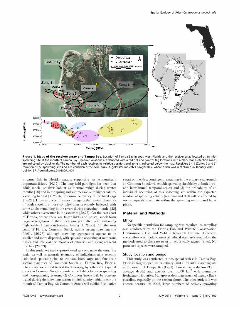
Figure 1. Maps of the receiver array and Tampa Bay. Location of Tampa Bay in southwest Florida and the receiver array located at an inletspawning site at the mouth of Tampa Bay. Receiver locations are denoted with a red dot and control tag locations with a black star. Detection zonesare indicated by black ovals. The number of each receiver, its relative position, and zone is indicated below the map. Receivers 3–19 (Zones 2 and 3)monitored the spawning site and are considered the core array. A gold star indicates Sawyer Key, where a fish was recaptured in January 2008.doi:10.1371/journal.pone.0101809.g001

Spatial Ecology of Adult Centropomus undecimalis


Common Snook were observed along the beach on the southern

shore of Shell Key (Lowerre-Barbieri, unpubl. data), which forms

the northern edge of the inlet (Fig. 1). The inlet is approximately

300 m across, with a relatively deep channel (maximum depth 8.5

m) bordered by sand bars. The bottom is predominantly shell

hash, with no submerged aquatic vegetation or oyster reefs and

currents are tidally-driven and can reach a maximum of 1 m/s (1.9

knots), decreasing as one moves eastward toward the estuary.

Individual snook (n = 31) sampled along the northern edge of the

inlet were acoustically tagged in June 2007 (see details below) and

passively monitored with a receiver array deployed at the inlet and

nearby areas. Twenty fish had tags that lasted 149 d and eleven

fish had three-year tags that remained active throughout the 2008

and 2009 spawning seasons.

Capture-based samplingEstuarine-wide Fishery-Independent Monitoring (FIM) of

Tampa Bay has been conducted monthly since 1996 using a

183-m haul seine and a stratified, random sampling design.

Sampling sites were selected from a sampling universe consisting of

one nautical mile square grids throughout Tampa Bay, which

included the inlet spawning site (see below). Tampa Bay was

divided into sampling zones based on logistical and hydrological

characteristics and each zone stratified into areas by habitat.

Monthly sampling was conducted at sites randomly selected from

the strata available for each zone [30]. Data recorded included:

abundance (including zeros, i.e. those hauls that did not catch

Common Snook), location and size, as well as salinity, water

temperature and the presence of bottom vegetation. We assessed

adult fish from this data set by selecting individuals with a standard

length (SL) $350 mm to be consistent with Winner et al. [29], but

this is considered conservative as Taylor et al. reported 50%

maturity at 250 mm total length (201 mm SL) [28].

Although the inlet spawning site was part of the FIM universe,

additional sampling was conducted here to assess reproductive

behavior. To evaluate the temporal pattern of snook presence and

spawning at this site, fish were captured with a 122-m knotless

center bag haul seine with 0.6 cm mesh, approximately weekly

from April through June. The haul seine was set along the beach,

corresponding to the northern edge of the core array (see Receiver

Array below). Prior to setting the net, we drove the length of the

beach to make visual observations of fish and/or courtship

behavior. Weather permitting, two net sets were made per date

and the net was retrieved immediately after deployment. Salinity

was measured each sampling date. Spawning activity of fish

captured at the inlet from April to June 2007 (n = 56) was

determined based on successful strip-spawning of males and

ovarian biopsies of females. Ovarian tissue was processed as

follows: fixed in 10% neutrally buffered formalin for 24 h, soaked

in water for 24 h, and stored in 70% ethanol. Samples were

embedded in glycol methacrylate, sectioned to 3–5-mm thickness,

stained with periodic acid–Schiff’s hematoxylin, and then coun-

terstained with metanil yellow [31]. Reproductive phases were

assigned following the criteria in Brown-Peterson et al. [32].

Receiver arrayWe deployed an array of 42 acoustic receivers (VR2s, Vemco

Ltd, Shad Bay, NS, Canada) to monitor the inlet and nearby areas

(Fig. 1). The array was an extension of that described in Lowerre-

Barbieri et al. 2013 [33] and designed so that a lack of detections

in the core array (Zones 2 and 3) corresponded to dates when fish

were not at the spawning site. The core array consisted of

seventeen receivers with overlapping ranges deployed off the

beach where Common Snook spawned. Long-term range testing

indicated that 85 m was the maximum range corresponding to

consistent detection (. 50%) at this site due to tidal currents [33].

Receivers were arranged so that all paths through the core array

were monitored by a minimum of three receivers. Another two

receivers were moored in the Gulf of Mexico < 200 m and < 400

m west of the core array. The remaining 23 receivers were

deployed nearby in the estuary (Fig. 1). Although this was not a

VPS (Vemco positioning system), the use of control tags [33–35],

allowed us to estimate position error [36] to determine if the

resolution of our data was sufficient for the hypotheses tested. We

deployed three control tags (69 kHz Vemco V9sc-2L 139 dB with

a 60 s fixed delay) in different zones (see below) within the array

(Fig. 1).

Fish taggingBecause we wanted to use telemetry to assess spawning site

fidelity, we did not implant any fish until spawning individuals

were captured in the haul seine samples referenced above. Fish

were sampled in the early evening (1735–2144 h) as this is the

expected time of spawning [15]. To decrease stress the bag of the

haul seine (2.4 m3) was kept submerged while by-catch items were

removed. Individual snook were kept continuously immersed in

transit from the net to the surgery station on the boat, by allowing

them to swim into a plastic sling. On the boat, fish were kept in a

live well (795 l capacity) until it was time for surgery. No more

than five fish were held at a time. To ensure the fish’s well-being,

the live well was set up as a flow-through system, allowing fish to

remain in ambient, oxygenated water [33]. Individuals selected for

surgery were removed from the live well after they voluntarily

swam into the sling.

A total of 31 snook (15F:16M) were intra-peritoneally implanted

with Vemco coded transmitters. Eleven fish (5F:6M) were

implanted with V13 tags (147 dB output, 540 d battery life, 30–

90 s random inter-pulse delay) and 20 fish (10F:10M) were

implanted with V9 tags (V9-2L-R, 146 dB output, 149 d battery

life, 15–45 s random inter-pulse delay). Based on the expected

spatio-temporal behavior of snook, the V13 tags were pro-

grammed to be active for 6 months (22 March through 20

September) to track fish during the spawning season (April-

September [15]) and inactive the remaining six months to

conserve battery life, allowing us to monitor snook over three

spawning seasons.

Fish implanted in June 2007 ranged in size from 495 to 792 mm

TL, with the average size of females (650 mm TL) being

significantly larger than that of males (591 mm TL; two-tailed t-

test, n = 31, P = 0.0308). Average surgery time was 7 m 20 s62 m

40 s SD. The surgical procedure followed that of Lowerre-Barbieri

et al.[33], with the exception that anesthesia was not used. Given

that Aqui-S is no longer approved for use in the United States with

food fish and these fish needed to be released immediately, an

alternative method to calm fish during surgery was needed.

Preliminary efforts indicated Common Snook responded well to

surgery when fish were calmed by being turned ventral side up and

having their eyes covered with a wet paper towel. Ambient,

oxygenated water was flushed over their gills throughout the

surgery. All males expressed milt on pressure and their reproduc-

tive phase was active spawning. Ovarian biopsies were taken from

all females prior to surgery for histological analysis of reproductive

state and the presence of spawning indicators [37,38]. Biopsies

were taken with a catheter composed of a 10 cc syringe equipped

with an adapter and Tygon tubing with an inner diameter of 1.6

mm. The tubing was inserted 10–20 mm into the urogenital pore

and the plunger of the syringe extended to create a vacuum to

extract oocytes. This method has been shown to be effective for



assessing reproductive state without the need for sacrificing the fish

(Lowerre-Barbieri unpubl. data). After surgery, all fish received an

external dart tag and were held in the live well for a minimum of

15 m before being released at the site of capture.

Data analysisTo understand the spatio-temporal patterns of snook estuary-

wide, catch rates from the FIM data were assessed using a two-part

hurdle model to account for zero-inflated data [39] with a

generalized linear model (GLM). Before building the model,

nominal CPUE data of snook $350 mm SL were plotted spatially

to determine if there were areas where snook catches were

concentrated in Tampa Bay and whether these areas differed with

the spawning season. Based on this analysis, Tampa Bay was

broken into two regions, one corresponding to high concentrations

of snook and the other to low concentrations during the spawning

season. These regions were spatially defined by performing a

kernel density estimate (KDE) on the spatial distribution of

nominal CPUE, selecting a contour of the KDE by which to

classify high versus low concentrations, and assigning each

sampling grid as either high versus low concentration (Fig. 2).

The two-part GLM consisted of (1) a presence-absence model that

estimated the proportion of hauls that caught snook (binomial

distribution with a logit link) and (2) a presence-only model that

estimated the number of snook $350 mm SL caught in an average

successful haul (log-normal distribution with an identity link).

Potential explanatory variables for both sub-models included year,

month, region (concentrated or not), spawning season (within:

April-September vs. outside: October-March), a region-by-spawn-

ing season interaction (i.e., to detect potential movements),

temperature grouped into 2.5uC bins, salinity grouped into

2.5% bins, and presence/absence of bottom vegetation. The

grouping of temperature and salinity was done to remove the

linear constraint from the models. The final set of sub-models was

chosen as the set with the lowest AIC using a stepwise forward-

selection procedure. Year was retained in all final sub-models to

obtain an index of abundance over time. Finally, year-specific,

marginal means estimates and their standard errors from the two

sub-models were used to generate distributions of estimates for

each sub-model from a Monte Carlo simulation (10,000 Student’s

t distributed realizations) and the product of these estimates after

back transforming from the log scales provided the distribution of

the catch rate with year-specific variability. All analyses were done

using R version 3.0.1 (R Development Core Team, 2011).

A database was developed in Access to integrate implantation

and detection data of acoustically tagged fish, with times reported

in Eastern Standard Time. Data were filtered to remove potential

spurious detections (n = 29) which were defined as a single

detection from a transmitter code (fish ID) in the core array over

a 24 h period [40]. Positions were estimated using the weighted

means method [41,42] with an hourly time bin (mean detections

per time bin equaled 9.660.09 SE) and based on two measures of

location: either UTM coordinates or VR2 receiver numbers. To

detect any abnormalities in behavior due to the stress of

implantation [33,36], data from the first 48 h (post-release period)

were analyzed separately. The study period was considered to start

after this initial 48 h. Two fish apparently died in 2009, i.e., they

exhibited no movement over an extended time period: tag 26

stopped moving on 10 June 2009 and tag 30 stopped moving on

25 June 2009. Detections from these tags were removed from the

data set after these dates, which resulted in 176,702 detections

used for subsequent analysis.

To simplify spatial interpretation, fish positions based on the

weighted means method were assigned to one of seven zones,

similar to the approach of Danylchuk et al. [43]. Zones 1–6 were

along the main channel to the inlet and within the estuary (Zone 1

being in the Gulf of Mexico and Zone 6 being the furthest within

the estuary, Fig. 1). Zone 7 was an area of shallower water to the

north of the main channel. The northern edge of Zones 2 and 3,

along the beach, corresponds to where spawning activity was

observed and actively spawning fish were sampled. Thus, the core

array was developed to cover Zones 2 and 3, and these zones are

referred to as the spawning site.

To assess the general spatial patterns of detected fish over the

three years, we plotted hourly positions of all fish by year. To test

whether the numbers of detections varied with zone, we used a

Chi-squared test. Residence time was calculated based on annual

total period of detection (TP, the number of days from the first

detection to the last detection for a given tag in a year) [44,45] and

estimated separately for the spawning site and non-spawning

zones. The number of days detected (DD) was also calculated.

Residence indices (RI) were estimated for the array (A) and for the

spawning site (SS) as the ratio of DD/TP for fish detected on five

or more dates. We used a Pearson’s correlation test to compare

RIA and RISS and a nonparametric Mann-Whitney test to assess

differences by sex.

To model the probability of detection within the spawning site

during the temporal window associated with spawning, we used a

generalized additive mixed model (GAMM) with a binomial

distribution (link = logit). Presence was coded as either 1 (present)

or 0 (absent) to identify fish detected within Zones 2 and 3 during

the spawning season and within the hours expected to correlate

with moving to the site and spawning (1400–2000 h). Analyses

were performed separately for all tagged fish in 2007 and for those

fish with three-year tags across all years. Explanatory variables

tested were: sex, sex-specific size (i.e., size was evaluated separately

for males and females due to the protandric life history of

Common Snook), detection date, and lunar phase, with year tested

in the multi-year analysis. Sex was included as a categorical

predictor and both day of the year and lunar phase were modeled

with cyclic cubic regression splines. For lunar phase, the predictor

was a continuous variable from 0 to 360 (full moon = 180, new

moon = 0 and 360). The use of alternative spline bases (thin plate

regression splines, cyclic P-splines) had a minimal effect on the

model. Because data were composed of repeated measures within

individuals, we considered its variability by including tag number

as a random factor [36]. The GAMM was fit using the gamm4

package [46] in R [47].

Results

Snook distribution in Tampa BayMore net sets captured snook during the spawning season than

in the non-spawning season, but snook were sampled in the

estuary year-round. A total of 4,920 seine hauls were conducted by

the FIM program in Tampa Bay from 1996 to 2012, and 34% of

these caught snook $350 mm SL. Snook occurred year-round in

areas close to shore throughout most of Tampa Bay (Fig. 2) but

were concentrated in three areas: on the eastern shore of the main

stem of Tampa Bay, on the eastern shore of the mouth of Old

Tampa Bay, and on the western shore at the mouth of Tampa Bay

(Fig. 2A, 2B). These areas were consequently grouped and defined

as a ‘‘concentrated’’ region. In the winter months, fish continued

to be present in the concentrated region but in lower numbers and

in fewer grids. The number of positive net sets modeled with the

binomial CPUE (lowest AIC = 5,884), included the following

explanatory variables: year, region (concentrated vs. not concen-

trated), temperature, and season (spawning vs. non-spawning).



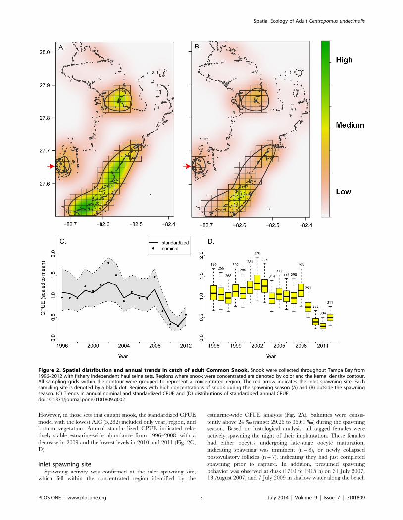
However, in those sets that caught snook, the standardized CPUE

model with the lowest AIC (5,282) included only year, region, and

bottom vegetation. Annual standardized CPUE indicated rela-

tively stable estuarine-wide abundance from 1996–2008, with a

decrease in 2009 and the lowest levels in 2010 and 2011 (Fig. 2C,

D).

Inlet spawning siteSpawning activity was confirmed at the inlet spawning site,

which fell within the concentrated region identified by the

estuarine-wide CPUE analysis (Fig. 2A). Salinities were consis-

tently above 24 % (range: 29.26 to 36.61 %) during the spawning

season. Based on histological analysis, all tagged females were

actively spawning the night of their implantation. These females

had either oocytes undergoing late-stage oocyte maturation,

indicating spawning was imminent (n = 8), or newly collapsed

postovulatory follicles (n = 7), indicating they had just completed

spawning prior to capture. In addition, presumed spawning

behavior was observed at dusk (1710 to 1915 h) on 31 July 2007,

13 August 2007, and 7 July 2009 in shallow water along the beach

Figure 2. Spatial distribution and annual trends in catch of adult Common Snook. Snook were collected throughout Tampa Bay from1996–2012 with fishery independent haul seine sets. Regions where snook were concentrated are denoted by color and the kernel density contour.All sampling grids within the contour were grouped to represent a concentrated region. The red arrow indicates the inlet spawning site. Eachsampling site is denoted by a black dot. Regions with high concentrations of snook during the spawning season (A) and (B) outside the spawningseason. (C) Trends in annual nominal and standardized CPUE and (D) distributions of standardized annual CPUE.doi:10.1371/journal.pone.0101809.g002



on the northern edge of the inlet, corresponding to the northern

edge of the core array (Zones 2 and 3). This behavior consisted of

‘‘balls’’ of five to seven fish, typically with one large fish assumed to

be female and multiple smaller fish assumed to be males. The fish

‘‘rolled’’ over each other and ‘‘flashed’’ white abdomens as they

traveled passively with the current in shallow water (, 2 m)

towards the Gulf of Mexico. Observed spawn times ranged from

1700 to 2000 h based on strip-spawning (mean = 1800 h, n = 4)

and ovulating females (n = 7) which were collected over the time

period from 1828 to 1942 h.

Some snook moved to the inlet prior to the spawning season.

Eleven snook were captured at the inlet in April and May 2007,

but no spawning indicators were observed until 22 May when the

first running ripe male was sampled. Ovarian biopsies from fish

captured in April (n = 4) confirmed that these females were not yet

spawning capable. The first spawning female was captured on 4

June.

Position error and fish survivalPosition errors in our array were less than the spatial scale of

interest (zone) and detection rates of all control tags were 99.7% or

better. Easting position error (mean and SE) of the control tags

increased towards the inlet (Zone 6: 10.9 m60.18 m; Zone 5: 39.2

m60.75 m; Zone 2: 85.9 m61.22 m) but positioning errors .200

m were rare in all zones (, 1%). The second spatial metric, mean

receiver number per hourly bin, exhibited lower error rates and

was used to plot individual movement paths. The pass control tag

(placed between receivers 9 and 10) resulted in a position based on

the mean receiver number of 9.5 to 10.560.05.

All fish survived the implantation process (n = 31), and thirty

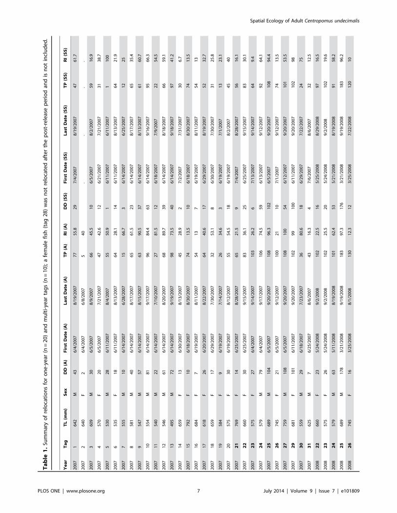
were relocated after the initial 48 h post-release period (Table 1).

On the date of implantation, fish (n = 25 detected) left the

spawning site within 4 hours of release. All fish were detected

moving towards the estuary and most of them were detected last at

receiver 23 (n = 20), just behind the tip of the barrier island (Zone

7).

Site fidelity and residence timesFish exhibited both intra-seasonal and inter-annual site fidelity,

repeatedly moving to and from the inlet spawning site within the

spawning season. Most fish (n = 28) detected in 2007 were

relocated on multiple dates in the spawning site (Table 1) and

all but one were detected for less than 24 h on any given date

(mean number of hours detected per date: 5.660.2 SE). Mean

DDSS of these fish was 39 d and ranged from 1 to 102 d. Ten fish

with multiple-year tags were detected in 2007. In 2008, nine of

these were detected and eight fish returned to the spawning site. In

2009, seven of these fish again returned and all seven fish were

relocated in the spawning site.

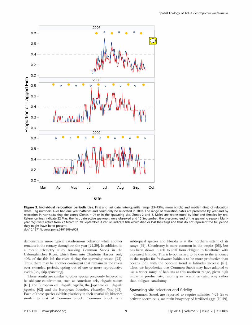
Most fish were detected in the array over a range of dates more

restricted than the period the tags were active (22 March through

20 September), but a few fish were detected over longer time

periods (Fig. 3, Table 1). In 2008, the majority of fish were first

detected both in the array and in the spawning site in mid-May.

However, three fish were detected in March: two males (tags 25

and 27) were consistently relocated throughout the period that the

tags were active and a female (tag 26) was detected one day in

March and then not again until May. These patterns remained

consistent in 2009. Even though V9 tags were active through

October 2007, the mean departure date for all three years was in

mid-August (2007: 16 August; 2008: 23 August; 2009: 19 August).

Because fish were implanted in June 2007, mean residence time

(TP) in that year was 65 d (n = 30), compared to approximately

four months in subsequent years (2008: 122 d, n = 9; 2009: 110 d,

n = 7), considerably less than the 184 d that tags were actively

transmitting. As mentioned above, two males exhibited a different

temporal pattern with TPs .180 d. Two recaptures of acoustically

tagged fish by anglers in late fall and winter also indicated some

fish remain in the area over longer time periods. Tag 18 (F) was

captured behind the barrier island near receiver 23 on 13 October

2009 and tag 31 (M) was captured at Sawyer Key on 12 January

2008 (Fig. 1).

Snook exhibited intra-seasonal fidelity to the inlet spawning site

but had varying relocation rates. RISS exhibited a strong

correlation with RIA (Pearson correlation coefficient = 0.90,

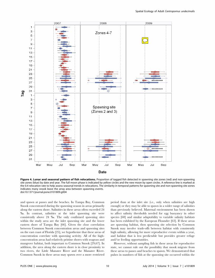
n = 38, P,0.0001). The proportion of fish detected repeatedly

spiked on dates near the new and full moons and then fell below

0.4 in between (Fig. 4). This temporal pattern in relocation rates

was similar for both spawning site zones and non-spawning site

zones, indicating many fish moved to and from the spawning site

over a larger spatial scale than monitored by the array. In 2007,

the proportion of fish relocated within the array on any given date

ranged from 0.03–0.70 (n = 1 to 21) with the most fish detected on

30 June. In 2008 and 2009, the relocation patterns were similar,

with the greatest number of fish detected in June, July, and August

and on dates near the new and full moons (Fig. 4). However,

seasonal patterns differed somewhat in their duration and peak

spawning period. In both 2007 and 2008, strong peaks occurred

early in the spawning season, with relocation rates decreasing as

the season progressed. In contrast, in 2009, peak relocation rates

remained relatively constant over a more extended spawning

season. Although both sexes had relatively high relocation rates,

male RIA values were significantly greater than female values

(Mann-Whitney Test U = 454, DF = 1, P,0.001), as were male

RISS values (Mann-Whitney Test U = 398; P,0.001, DF = 1;

Table 1).

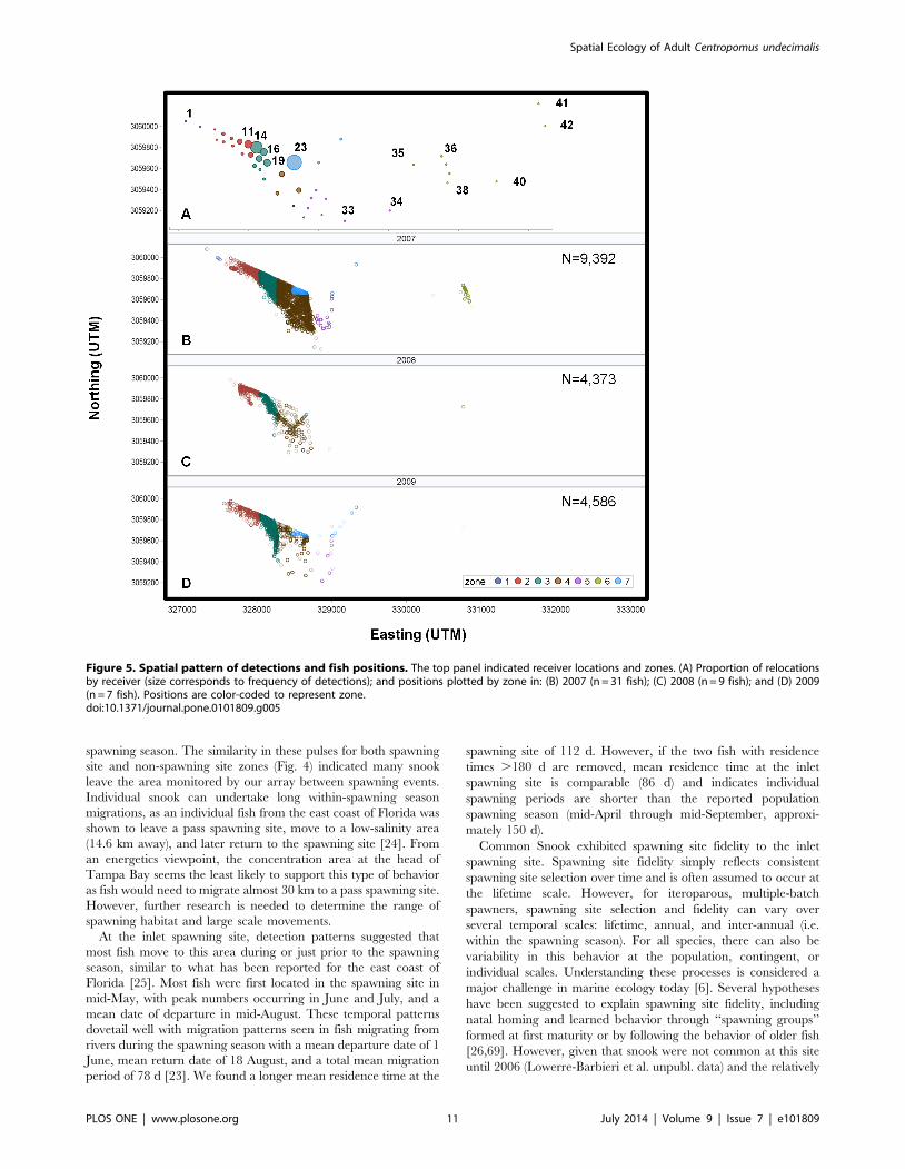
Movement patternsThe tagged fish exhibited similar spatial patterns over all three

years, with snook detected most frequently on receivers near the

barrier island and in Zones 2, 3, 4, and 7 (Fig. 5). Receiver 23,

behind the barrier island in Zone 7, had the highest proportion of

detections (0.32; Fig. 5A) with receiver 14 (in the spawning site,

Zone 3) having the second highest (0.20). Additional receivers

accounting for more than 2% of total detections were: receivers 21

and 24 in Zone 4 (cumulative 0.07), detecting fish as they moved

between the inlet spawning site and the area behind the barrier

island; receivers 19 (0.06) and 17 (0.07) in Zone 3, along the

eastern edge of the core array; and receivers 11 (0.08) and 9 (0.03)

in Zone 2 on the northern edge of the spawning site (Fig. 5A). For

zones with the greatest relocations (Zones 2, 3, 4, and 7),

detections were not equally distributed nor consistently affiliated

with zones with the greatest number of receivers (X2 = 3186.8, P,

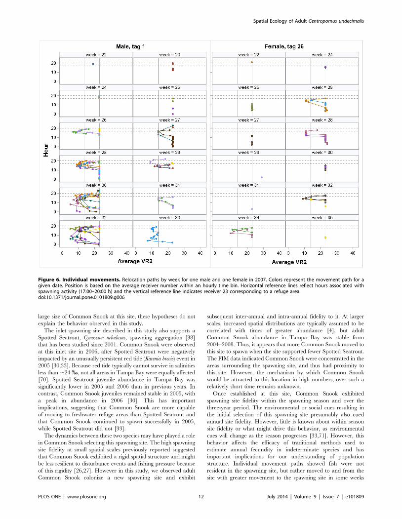
0.0001, DF = 3; Table 2). Individual daily movement paths helped

explain these patterns, as most individuals (n = 28) commonly

moved from the area behind the barrier island (detected at

receiver 23) to the inlet spawning site and back (Fig. 6). The area

monitored by receiver 23 appeared to act as a refuge, as fish were

commonly detected at this receiver for several weeks after

implantation and during hours not associated with spawning.

On some dates, movement to the inlet was associated with

spawning times, but on other dates fish moved to the inlet in the

early morning and did not leave until 2000 h or later.

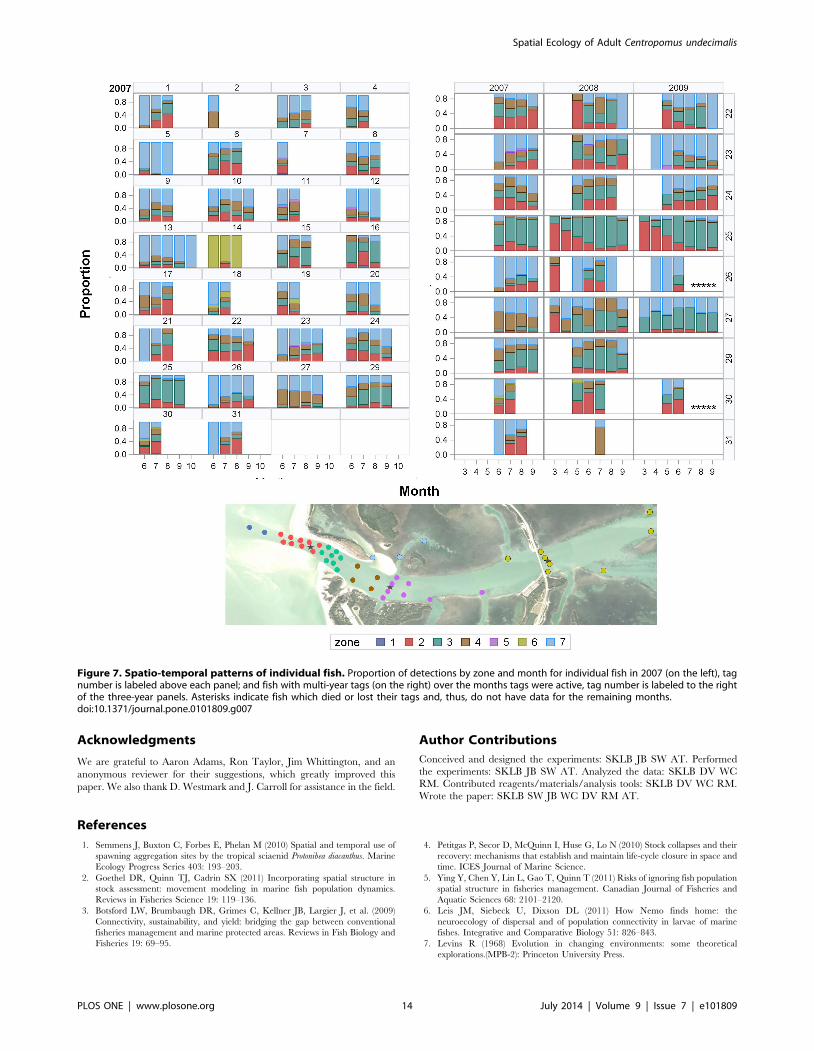
Individual spatio-temporal patterns indicated several contin-

gents. Although most fish were detected in zones associated with

the barrier island, one fish (tag 14) exhibited a spatial pattern

differing from the others, being predominantly relocated in Zone 6

(Fig. 7). The months of detection also differed by individual,



Ta

ble

1.

Sum

mar

yo

fre

loca

tio

ns

for

on

e-y

ear

(n=

20

)an

dm

ult

i-ye

arta

gs

(n=

10

);a

fem

ale

fish

(tag

28

)w

asn

ot

relo

cate

daf

ter

the

po

st-r

ele

ase

pe

rio

dan

dis

no

tin

clu

de

d.

Ye

ar

Ta

gT

L(m

m)

Se

xD

D(A

)F

irst

Da

te(A

)L

ast

Da

te(A

)T

P(A

)R

I(A

)D

D(S

S)

Fir

stD

ate

(SS

)L

ast

Da

te(S

S)

TP

(SS

)R

I(S

S)

20

07

16

42

M4

36

/4/2

00

78

/19

/20

07

77

55

.82

97

/4/2

00

78

/19

/20

07

47

61

.7

20

07

26

40

F2

6/4

/20

07

6/8

/20

07

54

0.

..

.

20

07

36

09

M3

06

/5/2

00

78

/9/2

00

76

64

5.5

10

6/5

/20

07

8/2

/20

07

59

16

.9

20

07

45

70

F2

06

/5/2

00

77

/21

/20

07

47

42

.61

26

/21

/20

07

7/2

1/2

00

73

13

8.7

20

07

55

30

M2

86

/11

/20

07

8/4

/20

07

55

50

.91

6/1

1/2

00

76

/11

/20

07

11

00

20

07

65

35

F1

86

/11

/20

07

8/1

3/2

00

76

42

8.1

14

6/1

1/2

00

78

/13

/20

07

64

21

.9

20

07

75

55

M1

06

/14

/20

07

6/2

8/2

00

71

56

6.7

36

/14

/20

07

6/2

5/2

00

71

22

5

20

07

85

81

M4

06

/14

/20

07

8/1

7/2

00

76

56

1.5

23

6/1

4/2

00

78

/17

/20

07

65

35

.4

20

07

95

47

M5

76

/14

/20

07

8/1

5/2

00

76

39

0.5

37

6/1

4/2

00

78

/13

/20

07

61

60

.7

20

07

10

55

4M

81

6/1

4/2

00

79

/17

/20

07

96

84

.46

36

/14

/20

07

9/1

6/2

00

79

56

6.3

20

07

11

54

0M

22

6/1

4/2

00

77

/10

/20

07

27

81

.51

26

/18

/20

07

7/9

/20

07

22

54

.5

20

07

12

54

6M

61

6/1

4/2

00

78

/20

/20

07

68

89

.73

96

/14

/20

07

8/1

8/2

00

76

65

9.1

20

07

13

49

5M

72

6/1

4/2

00

79

/19

/20

07

98

73

.54

06

/14

/20

07

9/1

8/2

00

79

74

1.2

20

07

14

65

9F

13

6/3

0/2

00

78

/13

/20

07

45

28

.92

7/2

/20

07

7/3

1/2

00

73

06

.7

20

07

15

79

2F

10

6/1

8/2

00

78

/30

/20

07

74

13

.51

06

/18

/20

07

8/3

0/2

00

77

41

3.5

20

07

16

68

4F

76

/19

/20

07

8/1

1/2

00

75

41

37

6/1

9/2

00

78

/11

/20

07

54

13

20

07

17

61

8F

26

6/2

0/2

00

78

/22

/20

07

64

40

.61

76

/29

/20

07

8/1

9/2

00

75

23

2.7

20

07

18

65

9F

17

6/2

9/2

00

77

/30

/20

07

32

53

.18

6/3

0/2

00

77

/30

/20

07

31

25

.8

20

07

19

58

4F

96

/19

/20

07

7/1

4/2

00

72

63

4.6

36

/19

/20

07

7/1

/20

07

13

23

.1

20

07

20

57

5F

30

6/1

9/2

00

78

/12

/20

07

55

54

.51

86

/19

/20

07

8/2

/20

07

45

40

20

07

21

76

9F

14

6/2

5/2

00

78

/28

/20

07

65

21

.59

7/4

/20

07

8/2

8/2

00

75

61

6.1

20

07

22

66

0F

30

6/2

5/2

00

79

/15

/20

07

83

36

.12

56

/25

/20

07

9/1

5/2

00

78

33

0.1

20

07

23

57

5F

27

6/4

/20

07

9/1

4/2

00

71

03

26

.26

7/1

3/2

00

79

/14

/20

07

64

9.4

20

07

24

57

9M

79

6/4

/20

07

9/1

7/2

00

71

06

74

.55

96

/13

/20

07

9/1

2/2

00

79

26

4.1

20

07

25

68

9M

10

46

/5/2

00

79

/20

/20

07

10

89

6.3

10

26

/5/2

00

79

/20

/20

07

10

89

4.4

20

07

26

74

5F

21

6/5

/20

07

9/1

2/2

00

71

00

21

10

7/1

/20

07

9/1

2/2

00

77

41

3.5

20

07

27

75

9M

10

86

/5/2

00

79

/20

/20

07

10

81

00

54

6/1

2/2

00

79

/20

/20

07

10

15

3.5

20

07

29

68

1F

10

16

/11

/20

07

9/2

0/2

00

71

02

99

10

06

/11

/20

07

9/2

0/2

00

71

02

98

20

07

30

55

9M

29

6/1

8/2

00

77

/23

/20

07

36

80

.61

86

/29

/20

07

7/2

2/2

00

72

47

5

20

07

31

62

5M

76

/25

/20

07

8/6

/20

07

43

16

.34

7/6

/20

07

8/6

/20

07

32

12

.5

20

08

22

66

0F

23

5/2

4/2

00

89

/2/2

00

81

02

22

.51

65

/25

/20

08

8/2

9/2

00

89

71

6.5

20

08

23

57

5F

26

5/2

4/2

00

89

/2/2

00

81

02

25

.52

05

/24

/20

08

9/2

/20

08

10

21

9.6

20

08

24

57

9M

63

5/1

1/2

00

88

/19

/20

08

10

16

2.4

53

5/2

1/2

00

88

/19

/20

08

91

58

.2

20

08

25

68

9M

17

83

/21

/20

08

9/1

9/2

00

81

83

97

.31

76

3/2

1/2

00

89

/19

/20

08

18

39

6.2

20

08

26

74

5F

16

3/2

5/2

00

88

/1/2

00

81

30

12

.31

23

/25

/20

08

7/2

2/2

00

81

20

10



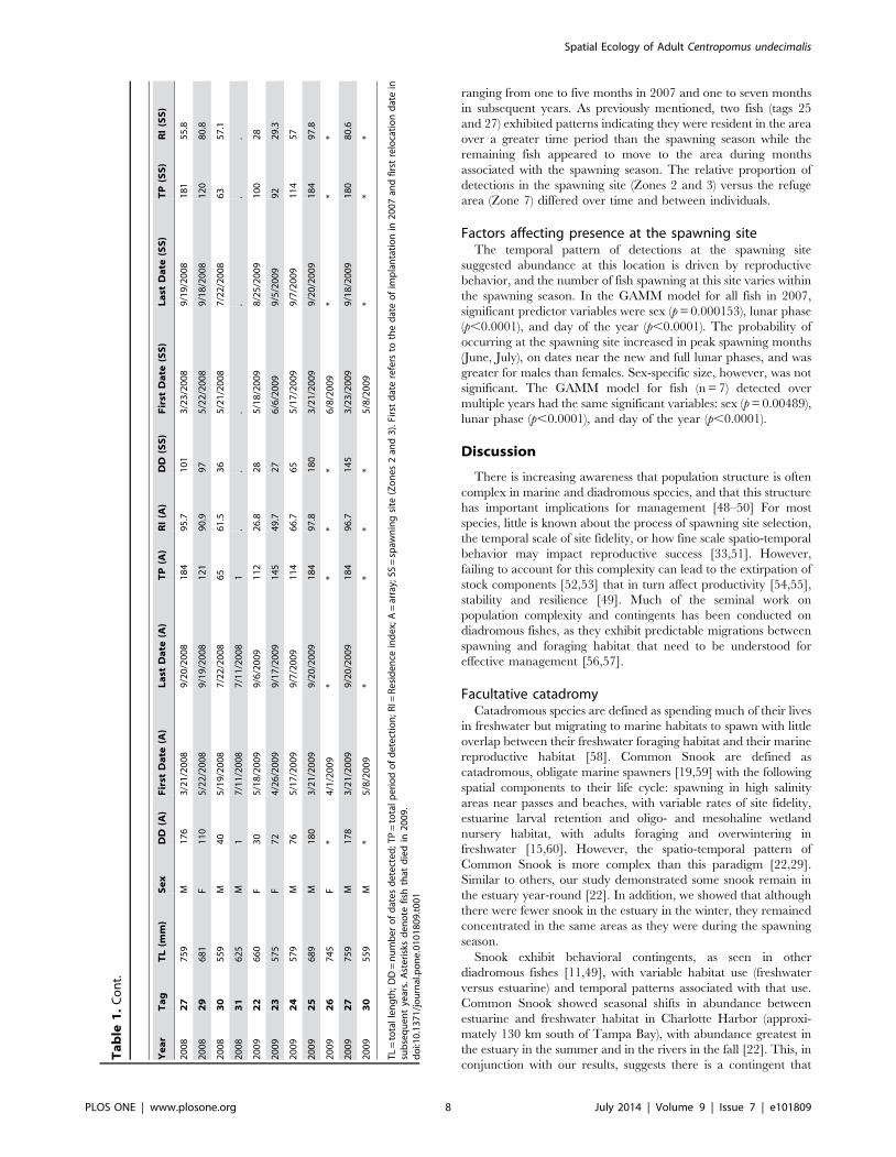
ranging from one to five months in 2007 and one to seven months

in subsequent years. As previously mentioned, two fish (tags 25

and 27) exhibited patterns indicating they were resident in the area

over a greater time period than the spawning season while the

remaining fish appeared to move to the area during months

associated with the spawning season. The relative proportion of

detections in the spawning site (Zones 2 and 3) versus the refuge

area (Zone 7) differed over time and between individuals.

Factors affecting presence at the spawning siteThe temporal pattern of detections at the spawning site

suggested abundance at this location is driven by reproductive

behavior, and the number of fish spawning at this site varies within

the spawning season. In the GAMM model for all fish in 2007,

significant predictor variables were sex (p = 0.000153), lunar phase

(p,0.0001), and day of the year (p,0.0001). The probability of

occurring at the spawning site increased in peak spawning months

(June, July), on dates near the new and full lunar phases, and was

greater for males than females. Sex-specific size, however, was not

significant. The GAMM model for fish (n = 7) detected over

multiple years had the same significant variables: sex (p = 0.00489),

lunar phase (p,0.0001), and day of the year (p,0.0001).

Discussion

There is increasing awareness that population structure is often

complex in marine and diadromous species, and that this structure

has important implications for management [48–50] For most

species, little is known about the process of spawning site selection,

the temporal scale of site fidelity, or how fine scale spatio-temporal

behavior may impact reproductive success [33,51]. However,

failing to account for this complexity can lead to the extirpation of

stock components [52,53] that in turn affect productivity [54,55],

stability and resilience [49]. Much of the seminal work on

population complexity and contingents has been conducted on

diadromous fishes, as they exhibit predictable migrations between

spawning and foraging habitat that need to be understood for

effective management [56,57].

Facultative catadromyCatadromous species are defined as spending much of their lives

in freshwater but migrating to marine habitats to spawn with little

overlap between their freshwater foraging habitat and their marine

reproductive habitat [58]. Common Snook are defined as

catadromous, obligate marine spawners [19,59] with the following

spatial components to their life cycle: spawning in high salinity

areas near passes and beaches, with variable rates of site fidelity,

estuarine larval retention and oligo- and mesohaline wetland

nursery habitat, with adults foraging and overwintering in

freshwater [15,60]. However, the spatio-temporal pattern of

Common Snook is more complex than this paradigm [22,29].

Similar to others, our study demonstrated some snook remain in

the estuary year-round [22]. In addition, we showed that although

there were fewer snook in the estuary in the winter, they remained

concentrated in the same areas as they were during the spawning

season.

Snook exhibit behavioral contingents, as seen in other

diadromous fishes [11,49], with variable habitat use (freshwater

versus estuarine) and temporal patterns associated with that use.

Common Snook showed seasonal shifts in abundance between

estuarine and freshwater habitat in Charlotte Harbor (approxi-

mately 130 km south of Tampa Bay), with abundance greatest in

the estuary in the summer and in the rivers in the fall [22]. This, in

conjunction with our results, suggests there is a contingent that

Ta

ble

1.

Co

nt.

Ye

ar

Ta

gT

L(m

m)

Se

xD

D(A

)F

irst

Da

te(A

)L

ast

Da

te(A

)T

P(A

)R

I(A

)D

D(S

S)

Fir

stD

ate

(SS

)L

ast

Da

te(S

S)

TP

(SS

)R

I(S

S)

20

08

27

75

9M

17

63

/21

/20

08

9/2

0/2

00

81

84

95

.71

01

3/2

3/2

00

89

/19

/20

08

18

15

5.8

20

08

29

68

1F

11

05

/22

/20

08

9/1

9/2

00

81

21

90

.99

75

/22

/20

08

9/1

8/2

00

81

20

80

.8

20

08

30

55

9M

40

5/1

9/2

00

87

/22

/20

08

65

61

.53

65

/21

/20

08

7/2

2/2

00

86

35

7.1

20

08

31

62

5M

17

/11

/20

08

7/1

1/2

00

81

..

..

..

20

09

22

66

0F

30

5/1

8/2

00

99

/6/2

00

91

12

26

.82

85

/18

/20

09

8/2

5/2

00

91

00

28

20

09

23

57

5F

72

4/2

6/2

00

99

/17

/20

09

14

54

9.7

27

6/6

/20

09

9/5

/20

09

92

29

.3

20

09

24

57

9M

76

5/1

7/2

00

99

/7/2

00

91

14

66

.76

55

/17

/20

09

9/7

/20

09

11

45

7

20

09

25

68

9M

18

03

/21

/20

09

9/2

0/2

00

91

84

97

.81

80

3/2

1/2

00

99

/20

/20

09

18

49

7.8

20

09

26

74

5F

*4

/1/2

00

9*

**

*6

/8/2

00

9*

**

20

09

27

75

9M

17

83

/21

/20

09

9/2

0/2

00

91

84

96

.71

45

3/2

3/2

00

99

/18

/20

09

18

08

0.6

20

09

30

55

9M

*5

/8/2

00

9*

**

*5

/8/2

00

9*

**

TL

=to

tal

len

gth

;D

D=

nu

mb

er

of

dat

es

de

tect

ed

;T

P=

tota

lp

eri

od

of

de

tect

ion

;R

I=R

esi

de

nce

ind

ex;

A=

arra

y;SS

=sp

awn

ing

site

(Zo

ne

s2

and

3).

Firs

td

ate

refe

rsto

the

dat

eo

fim

pla

nta

tio

nin

20

07

and

firs

tre

loca

tio

nd

ate

insu

bse

qu

en

tye

ars.

Ast

eri

sks

de

no

tefi

shth

atd

ied

in2

00

9.

do

i:10

.13

71

/jo

urn

al.p

on

e.0

10

18

09

.t0

01



demonstrates more typical catadromous behavior while another

remains in the estuary throughout the year [22,29]. In addition, in

a recent telemetry study tracking Common Snook in the

Caloosahatchee River, which flows into Charlotte Harbor, only

40% of the fish left the river during the spawning season [23].

Thus, there may be another contingent that remains in the rivers

over extended periods, opting out of one or more reproductive

cycles (i.e., skip spawning).

These results are similar to other species previously believed to

be obligate catadromous, such as American eels, Anguilla rostrata

[61], the European eel, Anguilla anguilla, the Japanese eel, Anguilla

japonica, [62] and the European flounder, Platichthys flesus [63].

Each of these species exhibits plasticity in their spatial life histories

similar to that of Common Snook. Common Snook is a

subtropical species and Florida is at the northern extent of its

range [64]. Catadromy is more common in the tropics [58], but

has been shown in eels to shift from obligate to facultative with

increased latitude. This is hypothesized to be due to the tendency

in the tropics for freshwater habitats to be more productive than

oceans [65], with the opposite trend as latitudes increase [61].

Thus, we hypothesize that Common Snook may have adapted to

use a wider range of habitats at this northern range, given high

estuarine productivity, resulting in facultative catadromy rather

than obligate catadromy.

Spawning site selection and fidelityCommon Snook are reported to require salinities .24 % to

activate sperm cells, maintain buoyancy of fertilized eggs [19,59],

Figure 3. Individual relocation periodicities. First and last date, inter-quartile range (25–75%), mean (circle) and median (line) of relocationdates. Tag numbers 1–20 had one year batteries and could only be relocated in 2007. The range of relocation dates are presented by year and byrelocation in non-spawning site zones (Zones 4–7) or in the spawning site, Zones 2 and 3. Males are represented by blue and females by red.Reference lines indicate 22 May, the first date active spawners were observed and 15 September, the presumed end of the spawning season. Multi-year tags were active from 22 March to 20 September. Asterisks indicate fish which died or lost their tags and thus do not represent the full periodthey might have been present.doi:10.1371/journal.pone.0101809.g003



Susan.Barbieri

Sticky Note

This graph panel belongs with figure 4

and spawn at passes and the beaches. In Tampa Bay, Common

Snook concentrated during the spawning season in areas primarily

along the eastern shore. Salinities in these areas often exceeded 24

%. In contrast, salinities at the inlet spawning site were

consistently above 24 %. The only confirmed spawning sites

within the study area are the inlet spawning site and the lower

eastern shore of Tampa Bay [66]. Given the close correlation

between Common Snook concentration areas and spawning sites

on the east coast of Florida [25], we hypothesize that these areas of

concentration correlate with spawning activity. All of the high-

concentration areas had relatively pristine shores with seagrass and

mangrove habitat, both important to Common Snook [29,67]. In

addition, the area along the eastern shore is in close proximity to

two rivers, the Little Manatee River and the Manatee River.

Common Snook in these areas may spawn over a more restricted

period than at the inlet site (i.e., only when salinities are high

enough) or they may be able to spawn in a wider range of salinities

than previously believed. Maternal environment has been shown

to affect salinity thresholds needed for egg buoyancy in other

species [68] and similar adaptability to variable salinity habitats

has been exhibited by the European Flounder [63]. If these areas

are spawning habitat, then spawning site selection by Common

Snook may involve trade-offs between habitat with consistently

high salinity, allowing for more reproductive events within a year,

and habitat that is less predictable but provides greater refuge

and/or feeding opportunities.

However, without sampling fish in these areas for reproductive

state, we cannot rule out the possibility that snook migrate from

these areas to passes and beaches to spawn. We demonstrated that

pulses in numbers of fish at the spawning site occurred within the

Figure 4. Lunar and seasonal pattern of fish relocations. Proportion of tagged fish detected in spawning site zones (red) and non-spawningsite zones (blue) by date and year. The full moon phase is indicated by yellow circles and the new moon by open circles. A reference line is marked atthe 0.4 relocation rate to help assess seasonal trends in relocations. The similarity in temporal patterns for spawning site and non-spawning site zonesindicates many snook leave the array area between spawning events.doi:10.1371/journal.pone.0101809.g004



Susan.Barbieri

Sticky Note

this graph panel belongs with figure 3.

spawning season. The similarity in these pulses for both spawning

site and non-spawning site zones (Fig. 4) indicated many snook

leave the area monitored by our array between spawning events.

Individual snook can undertake long within-spawning season

migrations, as an individual fish from the east coast of Florida was

shown to leave a pass spawning site, move to a low-salinity area

(14.6 km away), and later return to the spawning site [24]. From

an energetics viewpoint, the concentration area at the head of

Tampa Bay seems the least likely to support this type of behavior

as fish would need to migrate almost 30 km to a pass spawning site.

However, further research is needed to determine the range of

spawning habitat and large scale movements.

At the inlet spawning site, detection patterns suggested that

most fish move to this area during or just prior to the spawning

season, similar to what has been reported for the east coast of

Florida [25]. Most fish were first located in the spawning site in

mid-May, with peak numbers occurring in June and July, and a

mean date of departure in mid-August. These temporal patterns

dovetail well with migration patterns seen in fish migrating from

rivers during the spawning season with a mean departure date of 1

June, mean return date of 18 August, and a total mean migration

period of 78 d [23]. We found a longer mean residence time at the

spawning site of 112 d. However, if the two fish with residence

times .180 d are removed, mean residence time at the inlet

spawning site is comparable (86 d) and indicates individual

spawning periods are shorter than the reported population

spawning season (mid-April through mid-September, approxi-

mately 150 d).

Common Snook exhibited spawning site fidelity to the inlet

spawning site. Spawning site fidelity simply reflects consistent

spawning site selection over time and is often assumed to occur at

the lifetime scale. However, for iteroparous, multiple-batch

spawners, spawning site selection and fidelity can vary over

several temporal scales: lifetime, annual, and inter-annual (i.e.

within the spawning season). For all species, there can also be

variability in this behavior at the population, contingent, or

individual scales. Understanding these processes is considered a

major challenge in marine ecology today [6]. Several hypotheses

have been suggested to explain spawning site fidelity, including

natal homing and learned behavior through ‘‘spawning groups’’

formed at first maturity or by following the behavior of older fish

[26,69]. However, given that snook were not common at this site

until 2006 (Lowerre-Barbieri et al. unpubl. data) and the relatively

Figure 5. Spatial pattern of detections and fish positions. The top panel indicated receiver locations and zones. (A) Proportion of relocationsby receiver (size corresponds to frequency of detections); and positions plotted by zone in: (B) 2007 (n = 31 fish); (C) 2008 (n = 9 fish); and (D) 2009(n = 7 fish). Positions are color-coded to represent zone.doi:10.1371/journal.pone.0101809.g005



large size of Common Snook at this site, these hypotheses do not

explain the behavior observed in this study.

The inlet spawning site described in this study also supports a

Spotted Seatrout, Cynoscion nebulosus, spawning aggregation [38]

that has been studied since 2001. Common Snook were observed

at this inlet site in 2006, after Spotted Seatrout were negatively

impacted by an unusually persistent red tide (Karenia brevis) event in

2005 [30,33]. Because red tide typically cannot survive in salinities

less than ,24 %, not all areas in Tampa Bay were equally affected

[70]. Spotted Seatrout juvenile abundance in Tampa Bay was

significantly lower in 2005 and 2006 than in previous years. In

contrast, Common Snook juveniles remained stable in 2005, with

a peak in abundance in 2006 [30]. This has important

implications, suggesting that Common Snook are more capable

of moving to freshwater refuge areas than Spotted Seatrout and

that Common Snook continued to spawn successfully in 2005,

while Spotted Seatrout did not [33].

The dynamics between these two species may have played a role

in Common Snook selecting this spawning site. The high spawning

site fidelity at small spatial scales previously reported suggested

that Common Snook exhibited a rigid spatial structure and might

be less resilient to disturbance events and fishing pressure because

of this rigidity [26,27]. However in this study, we observed adult

Common Snook colonize a new spawning site and exhibit

subsequent inter-annual and intra-annual fidelity to it. At larger

scales, increased spatial distributions are typically assumed to be

correlated with times of greater abundance [4], but adult

Common Snook abundance in Tampa Bay was stable from

2004–2008. Thus, it appears that more Common Snook moved to

this site to spawn when the site supported fewer Spotted Seatrout.

The FIM data indicated Common Snook were concentrated in the

areas surrounding the spawning site, and thus had proximity to

this site. However, the mechanism by which Common Snook

would be attracted to this location in high numbers, over such a

relatively short time remains unknown.

Once established at this site, Common Snook exhibited

spawning site fidelity within the spawning season and over the

three-year period. The environmental or social cues resulting in

the initial selection of this spawning site presumably also cued

annual site fidelity. However, little is known about within season

site fidelity or what might drive this behavior, as environmental

cues will change as the season progresses [33,71]. However, this

behavior affects the efficacy of traditional methods used to

estimate annual fecundity in indeterminate species and has

important implications for our understanding of population

structure. Individual movement paths showed fish were not

resident in the spawning site, but rather moved to and from the

site with greater movement to the spawning site in some weeks

Figure 6. Individual movements. Relocation paths by week for one male and one female in 2007. Colors represent the movement path for agiven date. Position is based on the average receiver number within an hourly time bin. Horizontal reference lines reflect hours associated withspawning activity (17:00–20:00 h) and the vertical reference line indicates receiver 23 corresponding to a refuge area.doi:10.1371/journal.pone.0101809.g006



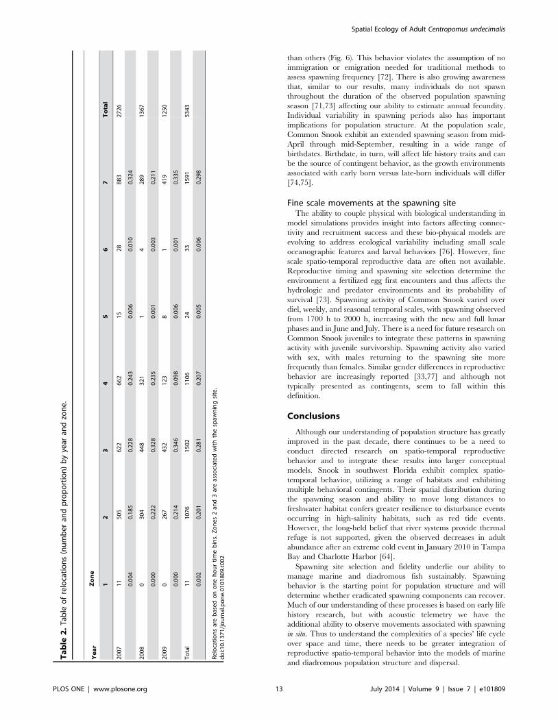
than others (Fig. 6). This behavior violates the assumption of no

immigration or emigration needed for traditional methods to

assess spawning frequency [72]. There is also growing awareness

that, similar to our results, many individuals do not spawn

throughout the duration of the observed population spawning

season [71,73] affecting our ability to estimate annual fecundity.

Individual variability in spawning periods also has important

implications for population structure. At the population scale,

Common Snook exhibit an extended spawning season from mid-

April through mid-September, resulting in a wide range of

birthdates. Birthdate, in turn, will affect life history traits and can

be the source of contingent behavior, as the growth environments

associated with early born versus late-born individuals will differ

[74,75].

Fine scale movements at the spawning siteThe ability to couple physical with biological understanding in

model simulations provides insight into factors affecting connec-

tivity and recruitment success and these bio-physical models are

evolving to address ecological variability including small scale

oceanographic features and larval behaviors [76]. However, fine

scale spatio-temporal reproductive data are often not available.

Reproductive timing and spawning site selection determine the

environment a fertilized egg first encounters and thus affects the

hydrologic and predator environments and its probability of

survival [73]. Spawning activity of Common Snook varied over

diel, weekly, and seasonal temporal scales, with spawning observed

from 1700 h to 2000 h, increasing with the new and full lunar

phases and in June and July. There is a need for future research on

Common Snook juveniles to integrate these patterns in spawning

activity with juvenile survivorship. Spawning activity also varied

with sex, with males returning to the spawning site more

frequently than females. Similar gender differences in reproductive

behavior are increasingly reported [33,77] and although not

typically presented as contingents, seem to fall within this

definition.

Conclusions

Although our understanding of population structure has greatly

improved in the past decade, there continues to be a need to

conduct directed research on spatio-temporal reproductive

behavior and to integrate these results into larger conceptual

models. Snook in southwest Florida exhibit complex spatio-

temporal behavior, utilizing a range of habitats and exhibiting

multiple behavioral contingents. Their spatial distribution during

the spawning season and ability to move long distances to

freshwater habitat confers greater resilience to disturbance events

occurring in high-salinity habitats, such as red tide events.

However, the long-held belief that river systems provide thermal

refuge is not supported, given the observed decreases in adult

abundance after an extreme cold event in January 2010 in Tampa

Bay and Charlotte Harbor [64].

Spawning site selection and fidelity underlie our ability to

manage marine and diadromous fish sustainably. Spawning

behavior is the starting point for population structure and will

determine whether eradicated spawning components can recover.

Much of our understanding of these processes is based on early life

history research, but with acoustic telemetry we have the

additional ability to observe movements associated with spawning

in situ. Thus to understand the complexities of a species’ life cycle

over space and time, there needs to be greater integration of

reproductive spatio-temporal behavior into the models of marine

and diadromous population structure and dispersal.

Ta

ble

2.

Tab

leo

fre

loca

tio

ns

(nu

mb

er

and

pro

po

rtio

n)

by

year

and

zon

e.

Ye

ar

Zo

ne

12

34

56

7T

ota

l

20

07

11

50

56

22

66

21

52

88

83

27

26

0.0

04

0.1

85

0.2

28

0.2

43

0.0

06

0.0

10

0.3

24

20

08

03

04

44

83

21

14

28

91

36

7

0.0

00

0.2

22

0.3

28

0.2

35

0.0

01

0.0

03

0.2

11

20

09

02

67

43

21

23

81

41

91

25

0

0.0

00

0.2

14

0.3

46

0.0

98

0.0

06

0.0

01

0.3

35

To

tal

11

10

76

15

02

11

06

24

33

15

91

53

43

0.0

02

0.2

01

0.2

81

0.2

07

0.0

05

0.0

06

0.2

98

Re

loca

tio

ns

are

bas

ed

on

on

eh

ou

rti

me

bin

s.Z

on

es

2an

d3

are

asso

ciat

ed

wit

hth

esp

awn

ing

site

.d

oi:1

0.1

37

1/j

ou

rnal

.po

ne

.01

01

80

9.t

00

2



Acknowledgments

We are grateful to Aaron Adams, Ron Taylor, Jim Whittington, and an

anonymous reviewer for their suggestions, which greatly improved this

paper. We also thank D. Westmark and J. Carroll for assistance in the field.

Author Contributions

Conceived and designed the experiments: SKLB JB SW AT. Performed

the experiments: SKLB JB SW AT. Analyzed the data: SKLB DV WC

RM. Contributed reagents/materials/analysis tools: SKLB DV WC RM.

Wrote the paper: SKLB SW JB WC DV RM AT.

References

1. Semmens J, Buxton C, Forbes E, Phelan M (2010) Spatial and temporal use of

spawning aggregation sites by the tropical sciaenid Protonibea diacanthus. Marine

Ecology Progress Series 403: 193–203.

2. Goethel DR, Quinn TJ, Cadrin SX (2011) Incorporating spatial structure in

stock assessment: movement modeling in marine fish population dynamics.

Reviews in Fisheries Science 19: 119–136.

3. Botsford LW, Brumbaugh DR, Grimes C, Kellner JB, Largier J, et al. (2009)

Connectivity, sustainability, and yield: bridging the gap between conventional

fisheries management and marine protected areas. Reviews in Fish Biology and

Fisheries 19: 69–95.

4. Petitgas P, Secor D, McQuinn I, Huse G, Lo N (2010) Stock collapses and their

recovery: mechanisms that establish and maintain life-cycle closure in space and

time. ICES Journal of Marine Science.

5. Ying Y, Chen Y, Lin L, Gao T, Quinn T (2011) Risks of ignoring fish population

spatial structure in fisheries management. Canadian Journal of Fisheries and

Aquatic Sciences 68: 2101–2120.

6. Leis JM, Siebeck U, Dixson DL (2011) How Nemo finds home: the

neuroecology of dispersal and of population connectivity in larvae of marine

fishes. Integrative and Comparative Biology 51: 826–843.

7. Levins R (1968) Evolution in changing environments: some theoretical

explorations.(MPB-2): Princeton University Press.

Figure 7. Spatio-temporal patterns of individual fish. Proportion of detections by zone and month for individual fish in 2007 (on the left), tagnumber is labeled above each panel; and fish with multi-year tags (on the right) over the months tags were active, tag number is labeled to the rightof the three-year panels. Asterisks indicate fish which died or lost their tags and, thus, do not have data for the remaining months.doi:10.1371/journal.pone.0101809.g007



8. Smedbol R, Wroblewski J (2002) Metapopulation theory and northern cod

population structure: interdependency of subpopulations in recovery of a

groundfish population. Fisheries Research 55: 161–174.

9. Hjort J. Fluctuations in the great fisheries of northern Europe viewed in the light

of biological research; 1914. ICES.

10. Clark J (1968) Seasonal movements of striped bass contingents of Long Island

Sound and the New York Bight. Transactions of the American Fisheries Society

97: 320–343.

11. Kraus T, Secor D (2004) Dynamics of white perch Morone americana population

contingents in the Patuxent River estuary, Maryland, USA. Marine Ecology

Progress Series 279: 247–259.

12. Cadrin SX, Secor DH (2009) Accounting for spatial population structure in

stock assessment: past, present, and future. The future of fisheries science in

North America: Springer. pp. 405–426.

13. Maunder MN, Deriso RB (2013) A stock–recruitment model for highly fecund

species based on temporal and spatial extent of spawning. Fisheries Research

146: 96–101.

14. Smedbol R, Stephenson R (2001) The importance of managing within-species

diversity in cod and herring fisheries of the north-western Atlantic. Journal of

Fish Biology 59: 109–128.

15. Taylor RG, Grier HJ, Whittington JA (1998) Spawning rhythms of common

snook in Florida. Journal of Fish Biology 53: 502–520.

16. Ley J, Allen M (2013) Modeling marine protected area value in a catch-and-

release dominated estuarine fishery. Fisheries Research 144: 60–73.

17. Muller RG, Taylor RG (2013) The 2013 stock assessment update of Common

Snook. St. Petersburg: Florida Fish and Wildlife Conservation Commission, Fish

andWildlife Research Institute.

18. Volpe AV (1959) Aspects of the biology of the common snook, Centropomus

undecimalis. Technical Series. St. Petersburg Florida: Florida State Board of

Conservation Marine Laboratory. pp. 38.

19. Ager LA, Hammond DE, Ware F (1976) Artificial spawning of snook.

Procedures of the Annual Conference of Southeastern Association of Fish and

Wildlife Agencies 30: 158–166.

20. Chapman P, Cross F, Fish W, Jones K (1982) Final report for sportfish

introductions projects. Study I. Artificial culture of snook. Florida Game and

Fesh Water Fish Commission. 1–36 p.

21. Peters KM, Matheson RE, Jr., Taylor RG (1998) Reproduction and early life

history of common snook, Centropomus undecimalis (Bloch), in Florida. Bulletin of

Marine Science 62: 509–529.

22. Blewett DA, Stevens PW, Champeau TR, R.G T (2009) Use of Rivers by

Common Snook Centropomus undecimalis in Southwest Florida: a first step in

addressing the Overrwintering Paradigm. Florida Scientist 72: 310–324.

23. Trotter AA, Blewett DA, Taylor RG, Stevens PW (2012) Migrations of

Common Snook from a tidal river with implications for skipped spawning.

Transactions of the American Fisheries Society 141: 1016–1025.

24. Lowerre-Barbieri SK, Vose FE, Whittington JA (2003) Catch-and-release fishing

on a spawning aggregation of common snook: Does it affect reproductive

output? Transactions of the American Fisheries Society 132: 940–952.

25. Young JM, Yeiser BG, Whittington JA (2014) Spatiotemporal dynamics of

spawning aggregations of common snook on the east coast of Florida. Marine

Ecology Progress Series (in press).

26. Adams A, Wolfe RK, Barkowski N, Overcash D (2009) Fidelity to spawning

grounds by a catadromous fish, Centropomus undecimalis. Marine Ecology Progress

Series 389: 213–222.

27. Adams AJ, Hill JE, Samoray C (2011) Characteristics of spawning ground

fidelity by a diadromous fish: a multi-year perspective. Environmental Biology of

Fishes: 1–9.

28. Taylor RG, J.A.. Whittington, H.J.. Grier, R.E.Crabtree (2000) Age, growth,

maturation, and protandric sex reversal in common snook, Centropomus

undecimalis, from the east and west coasts of South Florida. Fishery Bulletin 98:

612–624.

29. Winner BL, Blewett DA, McMichael Jr RH, Guenther CB (2010) Relative

abundance and distribution of common snook along shoreline habitats of Florida

estuaries. Transactions of the American Fisheries Society 139: 62–79.

30. Flaherty K, Landsberg J (2011) Effects of a persistent red tide (Karenia brevis)

bloom on community structure and species-specific relative abundance of nekton

in a Gulf of Mexico estuary. Estuaries and Coasts 34: 417–439.

31. Quintero-Hunter I, Grier H, Muscato M (1991) Enhancement of histological

detail using metanil yellow as counterstain in periodic acid Schiff’s hematoxylin

staining of glycol methacrylate tissue sections. Biotechnic & Histochemistry 66:

169–172.

32. Lowerre-Barbieri S, Brown-Peterson N, Murua H, Tomkiewicz J, Wyanski D, et

al. (2011) Emerging issues and methodological advances in fisheries reproductive

biology. Marine and Coastal Fisheries: Dynamics. Management, and Ecosystem

Science [online serial] 3: 32–51.

33. Lowerre-Barbieri SK, Walters S, Bickford J, Cooper W, Muller R (2013) Site

fidelity and reproductive timing at a Spotted Seatrout spawning aggregation site:

individual versus population scale behavior. Marine Ecology Progress Series 481:

181–197.

34. Villegas-Rıos D, Alos J, March D, Palmer M, Mucientes G, et al. (2013) Home

range and diel behavior of the ballan wrasse, Labrus bergylta, determined by

acoustic telemetry. Journal of Sea Research 80: 61–71.

35. Payne NL, Gillanders BM, Webber DM, Semmens JM (2010) Interpreting dielactivity patterns from acoustic telemetry: the need for controls. Marine Ecology

Progress Series 419: 295–301.

36. Alos J, Cabanellas-Reboredo M, Lowerre-Barbieri SK (2012) Diel behaviourand habitat utilisation by the pearly razorfish during the spawning season.

Marine Ecology Progress Series 460: 207–220.

37. Brown-Peterson N, Wyanski D, Saborido-Rey F, Macewicz B, Lowerre-BarbieriS (2011) A standardized terminology for describing reproductive development in

fishes. Marine and Coastal Fisheries: Dynamics. Management, and EcosystemScience [online serial] 3: 52–70.

38. Lowerre-Barbieri SK, Henderson N, Llopiz J, Walters S, Bickford J, et al. (2009)

Defining a spawning population(Spotted Seatrout Cynoscion nebulosus) overtemporal, spatial, and demographic scales. Marine Ecology Progress Series

394: 231–245.

39. Zuur A, Ieno E, Walker N, Saveliev A, Smith G (2009) Mixed effects models andextensions in ecology with R. New York: Springer.

40. Meyer CG, Burgess WC, Papastamatiou YP, Holland KN (2007) Use of an

implanted sound recording device (Bioacoustic Probe) to document the acousticenvironment of a blacktip reef shark (Carcharhinus melanopterus). Aquatic Living

Resources 20: 291–298.

41. Simpfendorfer CA, Heupel MR, Hueter RE (2002) Estimation of short-termcenters of activity from an array of omnidirectional hydrophones and its use in

studying animal movements. Canadian Journal of Fisheries and AquaticSciences 59: 23–32.

42. Hedger RD, Martin F, Dodson JJ, Hatin D, Caron F, et al. (2008) The

optimized interpolation of fish positions and speeds in an array of fixed acousticreceivers. ICES Journal of Marine Science: Journal du Conseil 65: 1248–1259.

43. Danylchuk A, Cooke S, Goldberg T, Suski C, Murchie K, et al. (2011)

Aggregations and offshore movements as indicators of spawning activity ofbonefish (Albula vulpes) in The Bahamas. Marine Biology 158: 1981–1999.

44. March D, Palmer M, Alos J, Grau A, Cardona F (2010) Short-term residence,

home range size and diel patterns of the painted comber Serranus scriba in atemperate marine reserve. Marine Ecology Progress Series 400: 195–206.

45. Palmer M, Balle S, March D, Alos J, Linde M (2011) Size estimation of circular

home range from fish mark-release-(single)-recapture data: case study of a smalllabrid targeted by recreational fishing. Marine Ecology Progress Series 430: 87–

97.

46. Wood S, Scheipl F (2013) Generalized additive mixed models using mgcv andIme4. R package version 02–1.

47. R Development Core Team (2013) R: A language and environment for

statistical computing. Vienna, Austria: R Foundation for Statistical Computing.

48. Secor D (1999) Specifying divergent migrations in the concept of stock: the

contingent hypothesis. Fisheries Research 43: 13–34.

49. Kerr LA, Cadrin SX, Secor DH (2010) The role of spatial dynamics in thestability, resilience, and productivity of an estuarine fish population. Ecological

Applications 20: 497–507.

50. Cardinale M, Bartolino V, Llope M, Maiorano L, Skold M, et al. (2011)Historical spatial baselines in conservation and management of marine

resources. Fish and Fisheries 12: 289–298.

51. Berkeley SA, Hixon MA, Larson RJ, Love MS (2004) Fisheries sustainability viaprotection of age atructure and spatial distribution of fish populations. Fisheries

29: 23–32.

52. Frank KT, Brickman D (2001) Contemporary management issues confronting

fisheries science. J Sea Research 45: 173–187.

53. Hutchinson WF, van Oosterhout C, Rogers SI, Carvalho GR (2003) Temporalanalysis of archived samples indicates marked genetic changes in declining North

Sea cod (Gadus morhua). Proceedings of the Royal Society of London Series B:

Biological Sciences 270: 2125–2132.

54. Svedang H, Righton D, Jonsson P (2007) Migratory behaviour of Atlantic cod

Gadus morhua: natal homing is the prime stock-separating mechanism. Marine


55. Svedang H, Andre C, Jonsson P, Elfman M, Limburg KE (2010) Migratory

behaviour and otolith chemistry suggest fine-scale sub-population structurewithin a genetically homogenous Atlantic Cod population. Environmental

biology of fishes 89: 383–397.

56. Walsh CT, Reinfelds IV, Gray CA, West RJ, van der Meulen DE, et al. (2012)Seasonal residency and movement patterns of two co-occurring catadromous

percichthyids within a south-eastern Australian river. Ecology of Freshwater Fish

21: 145–159.

57. Miles NG, Walsh CT, Butler G, Ueda H, West RJ (2014) Australian diadromous

fishes ? challenges and solutions for understanding migrations in the 21st

century. Marine and Freshwater Research 65: 12–24.

58. McDowall RM (1997) The evolution of diadromy in fishes (revisited) and its

place in phylogenetic analysis. Reviews in Fish Biology and Fisheries 7: 443–462.

59. Tucker JW, Jr. (1987) Snook and tarpon snook culture and preliminaryevaluation for commercial farming. The Progressive Fish Culturist 49: 49–57.

60. Barbour AB, Adams AJ (2012) Biologging to examine multiple life stages of an

estuarine-dependent fish. Marine Ecology Progress Series.

61. Thibault I, Dodson JJ, Caron F, Tzeng W, Iizuka Y, et al. (2007) Facultative

catadromy in American eels: testing the conditional strategy hypothesis. Marine


62. Daverat F, Limburg KE, Thibault I, Shiao J-C, Dodson JJ, et al. (2006)

Phenotypic plasticity of habitat use by three temperate eel species, Anguilla

anguilla, A. japonica and A. rostrata. Marine Ecology Progress Series 308: 231–241.



63. Daverat F, Morais P, Dias E, Babaluk J, Martin J, et al. (2012) Plasticity of

European flounder life history patterns discloses alternatives to catadromy.

Marine Ecology Progress Series 465: 267–280.

64. Adams AJ, Hill JE, Kurth BN, Barbour AB (2012) Effects of a severe cold event

on the subtropical, estuarine-dependent common snook, Centropomus undecimalis.

Gulf and Caribbean Research 24: 13–21.

65. Gross MR, Coleman RM, McDowall RM (1988) Aquatic productivity and the

evolution of diadromous fish migration. Science(Washington) 239: 1291–1293.

66. Yanes-Roca C, Rhody N, Nystrom M, Main KL (2009) Effects of fatty acid

composition and spawning season patterns on egg quality and larval survival in

common snook (Centropomus undecimalis). Aquaculture 287: 335–340.

67. Blewett DA, Hensley RA, Stevens PW, Fish F (2006) Feeding habits of common

snook, Centropomus undecimalis, in Charlotte Harbor, Florida. Gulf and Caribbean

Research 18: 1.

68. Kucera C (2002) The effect of parental acclimation to spawning salinity on the

survival of larval Cynoscion nebulosus. Journal of Fish Biology 61: 726–738.

69. Colin PL (1996) Longevity of some coral reef fish spawning aggregations. Copeia

1996: 189–192.

70. Walters S, Lowerre-Barbieri S, Bickford J, Tustison J, Landsberg JH (2013)

Effects of Karenia brevis red tide on the spatial distribution of spawning

aggregations of sand seatrout Cynoscion arenarius in Tampa Bay, Florida. Marine


71. Bijoux J, Dagorn L, Berke G, Cowley P, Soria M, et al. (2013) Temporal

dynamics, residency and site fidelity of spawning aggregations of a herbivoroustropical reef fish Siganus sutor. Marine Ecology Progress Series 475: 233–247.

72. Hunter JR, Macewicz BJ (1985) Measurement of spawning frequency in multiple

spawning fishes. In: Lasker R, editor. An egg production method for estimatingspawning biomass of pelagic fishes: application to the northern anchovy,

Engraulis mordax NOAA Technical Report NMFS. pp. 79–94.73. Lowerre-Barbieri S, Ganias K, Saborido-Rey F, Murua H, Hunter J (2011)

Reproductive timing in marine fishes: variability, temporal scales, and methods.

Marine and Coastal Fisheries: Dynamics. Management, and Ecosystem Science[online serial] 3: 71–91.

74. Lowerre-Barbieri SK, Lowerre JM, Barbieri LR (1998) Multiple spawning andthe dynamics of fish populations: inferences from an individual-based simulation

model. Canadian Journal of Fisheries and Aquatic Sciences 55: 2244–2254.75. Lozano C, Houde ED, Wingate RL, Secor DH (2012) Age, growth and hatch

dates of ingressing larvae and surviving juveniles of Atlantic menhaden Brevoortia

tyrannus. Jounral of Fish Biology 81: 1665–1685.76. Paris CB, Helgers J, van Sebille E, Srinivasan A (2013) Connectivity Modeling

System: A probabilistic modeling tool for the multi-scale tracking of biotic andabiotic variability in the ocean. Environmental Modelling & Software 42: 47–54.

77. Claydon J (2004) Spawning aggregations of coral reef fishes: characteristics,

hypotheses, threats and management. Marine Biology Annual Review 42: 265–302.



Spawning Site Selection and Contingent Behavior in Common Snook, Centropomus undecimalis

Documents

Transcript of Spawning Site Selection and Contingent Behavior in Common Snook, Centropomus undecimalis