Contingent valuation with heterogeneous reasonsfor uncertainty

Daniel R. Petrolia a,*, Tae-Goun Kim b,1

a Department of Agricultural Economics, Mississippi State University, Box 5187, Mississippi State, MS 39762, United Statesb Division of Maritime Transportation Science, Korea Maritime University, 1 Dongsam-dong, Youngdo-Gu, Busan 606-791, South Korea

1. Introduction

There has been much work over the past 15 years investigating the benefits of incorporatingrespondent uncertainty into contingent-valuation models. This has been in response to therecommendations of Arrow et al. (1993), that contingent-valuation referenda should include a ‘‘wouldnot vote’’ choice in addition to ‘‘yes’’ and ‘‘no’’. Out of this recommendation followed a number of variantsof the ‘‘would not vote/I don’t know’’ choice. For example, Li and Mattsson (1995) introduced a follow-upquestion asking respondents to indicate their level of confidence in their answer, and then using thisadditional information to improve value estimates. Wang (1997) proposed a model that assumes that

Resource and Energy Economics 33 (2011) 515–526

A R T I C L E I N F O

Article history:

Received 30 November 2009

Received in revised form 28 September 2010

Accepted 21 October 2010

Available online 30 October 2010

JEL classification:

Q51

Keywords:

Barrier islands

Cheap talk

Coastal restoration

Contingent valuation

Survey

Willingness to pay

A B S T R A C T

We test the hypothesis that respondents stating divergent reasons

for choice uncertainty differ in their probability to vote yes in a CV

setting. We introduce the use of a follow-up question used to

classify uncertain respondents according to reason for uncertainty.

Results indicate that respondents whose uncertainty derived from

concerns about unforeseen negative impacts associated with

provision of the good were more likely to vote yes, and depending

on the model, that the probability of a yes vote of these respondents

was consistently different than that of respondents whose

uncertainty derived from concern about cost of provision or

expected benefits.

� 2010 Elsevier B.V. All rights reserved.

* Corresponding author. Tel.: +1 662 325 2888; fax: +1 662 325 8777.

E-mail addresses: petrolia@agecon.msstate.edu (D.R. Petrolia), teddykim48@hhu.ac.kr (T.-G. Kim).1 Tel.: +82 51 410 4437.

Contents lists available at ScienceDirect

Resource and Energy Economics

journal homepage: www.e lsev ier .com/ locate / ree

0928-7655/$ – see front matter � 2010 Elsevier B.V. All rights reserved.

doi:10.1016/j.reseneeco.2010.10.001

respondents hold an implicit valuation distribution rather than a single true value, and that if an offeredbid is not clearly different from the mean value of one’s valuation distribution, the respondent may give a‘‘don’t know’’ answer. Loomis and Ekstrand (1998) proposed coding responses on a continuum between0 and 1 based on respondents stated certainty level rather than restricting the dependent variable to bebinary. Welsh and Poe (1998) developed a multiple-bounded polychotomous-choice technique thatallowed respondents to express their level of certainty explicitly within the question itself, answering‘‘definitely no’’, ‘‘probably no’’, ‘‘not sure’’, etc., rather than simply ‘‘yes’’ or ‘‘no’’.

However, the problem then arose as to what to do with such responses. Carson et al. (1998b) note thatthere are at least three interpretations describing how people would respond to a CV question thatincluded the ‘‘would not vote/not sure’’ option. Two of these would leave the marginal distributions ofthe ‘‘yes’’ and ‘‘no’’ categories unaffected (i.e., the ‘‘would not vote’’ option would attract responses inequal proportion from the ‘‘yes’’ and ‘‘no’’ categories), whereas the third interpretation would have adisproportionate number of ‘‘would not vote’’ responses coming from the ‘‘yes’’ category. Based on theirown estimates, however, they concluded that ‘‘would not vote’’ responses would have voted ‘‘no’’ in theabsence of the ‘‘would not vote’’ option. Comparing results of the multiple-bounded and single-boundeddichotomous-choice techniques, Welsh and Poe (1998) found that, ceteris paribus, when respondents to asingle dichotomous-choice question are unsure of their vote, they are likely to report a ‘‘yes’’ vote, i.e.,engage in ‘‘yea-saying’’. Ready et al. (2001) found that if respondents were told the degree of certainty onwhich to base their response, then the responses under alternative question formats converged. Alberiniet al. (2003), however, indicate that their results support neither the findings of Carson et al. (1998b) norWelsh and Poe (1998). They found that, in the absence of uncertain choices, people who would haveanswered ‘‘definitely yes’’ or ‘‘probably yes’’ would choose to answer ‘‘yes’’. I.e., they conclude that ‘‘yes’’responses from uncertain respondents are ‘‘true’’ ‘‘yes’’ responses, not merely yea-saying. More recently,Flachaire and Hollard (2007), who, applying the Range Model to the same Exxon Valdez dataset as Carsonet al. (1998b), found that when uncertain, individuals tend to answer ‘‘yes’’, thus reversing the findings ofCarson et al. Additionally, Broberg and Brannlund (2008) recently hypothesized that uncertainindividuals would like to state their WTP as intervals rather than precise values and that the width of theintervals is determined by the degree of uncertainty.

Alberini et al. (2003) concluded their paper by saying that ‘‘Our findings, and the contrast betweenour findings and those of previous studies that have allowed uncertain responses, suggest that moreconsideration needs to be given to the framing of the questions and response formats that allow foruncertainty, and the reasons people choose to give responses that indicate uncertainty’’ (p. 59).However, we find that little to no attention has been paid to the latter issue, i.e., the reasons peoplechoose to give uncertain responses. In this study, we hypothesize that the expected response of anuncertain respondent is a function of the reason behind the uncertainty. Thus, it may not beappropriate to assume either that all uncertain responses are truly ‘‘yes’’ votes or ‘‘no’’ votes, but ratherthat some are ‘‘yes’’ votes and some are ‘‘no’’ votes. This could be at least one possible explanation forthe contradictory findings described above.

We test our hypothesis on data from a survey on WTP for barrier-island restoration in Mississippi. Weintroduced a follow-up question to a CV referendum that attempts to classify uncertain respondents byparticular uncertainty types, and then incorporated this information into various models of WTP to testfor significant differences in expected response across types, while controlling for other factors. Ourresults indicate that respondents whose uncertainty derived from concerns about potentiallyunforeseen negative impacts associated with provision of the good were more likely to vote ‘‘yes’’relative to respondents with complete certainty. Further, we have weak evidence that those whoseuncertainty derived from concerns about cost (i.e., budgetary) concerns or concerns about the expectedbenefits of the good, were less likely to vote ‘‘yes’’. Those whose uncertainty was derived from some othersource, such as distrust of government or dissatisfaction with the payment mechanism, etc., were foundto be neither more nor less likely to vote ‘‘yes’’ relative to respondents with complete certainty.

2. Methods

The public good selected for this analysis was restoration of the Mississippi barrier-island chain,which is currently being considered by the State of Mississippi and U.S. Corps of Engineers. The chain

D.R. Petrolia, T.-G. Kim / Resource and Energy Economics 33 (2011) 515–526516

consists of five distinct islands: Cat, West Ship, East Ship, Horn, and Petit Bois. These islands likelyoriginated as submerged sand shoals that emerged from the Gulf of Mexico and aggraded as sea levelrose (Morton, 2007). They lie roughly parallel to the coast, between 9 and 12 miles offshore, and,combined, contain 6545 acres of land mass (Carter and Blossom, 2007). According to Morton (2007),the islands are undergoing rapid land loss and translocation, the principal causes of which are frequentintense storms, a relative rise in sea level, and a deficit in the sediment budget. However, the onlyfactor that has a historical trend that coincides with the progressive increase in rates of land loss is theprogressive reduction in sand supply associated with nearly-simultaneous deepening of channels fordeep-draft shipping. Neither rates of relative sea level rise nor storm parameters have long-termhistorical trends that match the increased rates of land loss since the mid-1800s. The most recent landloss acceleration, however, is likely related to increased storm activity since 1995 (Morton, 2007).

The survey instrument was designed to collect data on WTP for three different scales of restoration.The three hypothetical restoration options were constructed based on data obtained from Carter andBlossom (2007). Each restoration scale proposed to restore a given number of acres of land mass to theislands’ footprint and maintain them for a 30-year period. Specifically, the three scales were: the Status-Quo scale (small scale), which would maintain the current island footprint for a 30-year period; the Pre-Camille scale (medium), which would restore the islands to their Pre-Hurricane Camille (1969)footprint; and the Pre-1900 scale (large), which would restore the islands to their Pre-1900 footprint. Thethree restoration scales were presented to every respondent, one-by-one, followed by a dichotomous-choice referendum-style question of support for each option at the stated one-time bid versus no action.

Five bids were used for each restoration scale, based on barrier-island restoration cost estimatestaken from T. Baker Smith and Sons, Inc. (1997) and adjusted for inflation. Bids varied across surveysand were set as 50%, 100%, 150%, 200%, and 250% of baseline cost per taxpaying Mississippi household.Specifically, the bids were one-time payments of $7, $13, $20, $26, and $33 for the Status-Quo scale;$77, $153, $230, $306, and $383 for the Pre-Camille scale; and $195, $391, $586, $782, and $977 for thePre-1900 scale. Each respondent was presented with the same relative bids across the three options;e.g., a respondent that was presented the highest bid at the small scale was also presented the highestbid at the other two scales. This was done to keep the number of survey versions manageable given theother treatments in which we were interested.

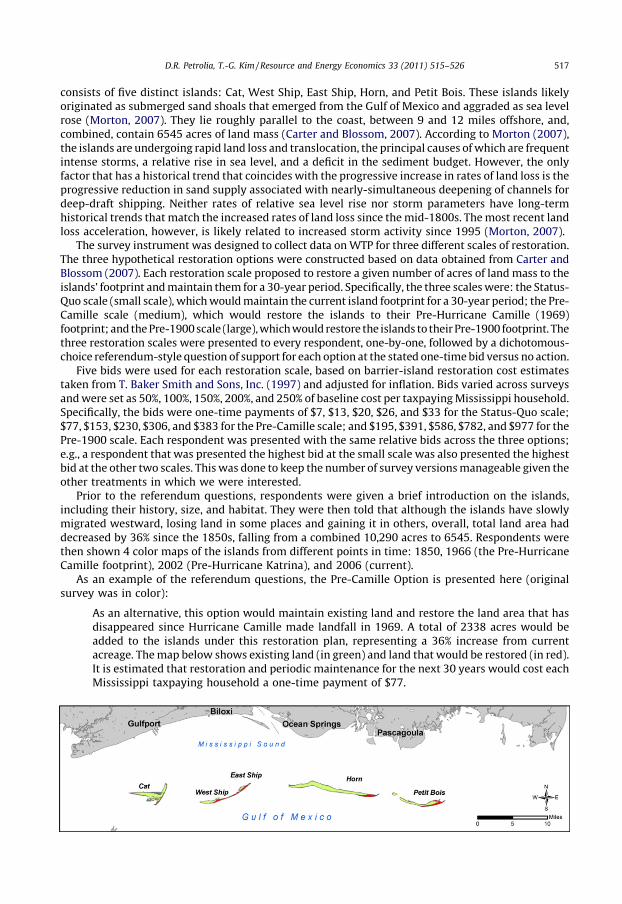
Prior to the referendum questions, respondents were given a brief introduction on the islands,including their history, size, and habitat. They were then told that although the islands have slowlymigrated westward, losing land in some places and gaining it in others, overall, total land area haddecreased by 36% since the 1850s, falling from a combined 10,290 acres to 6545. Respondents werethen shown 4 color maps of the islands from different points in time: 1850, 1966 (the Pre-HurricaneCamille footprint), 2002 (Pre-Hurricane Katrina), and 2006 (current).

As an example of the referendum questions, the Pre-Camille Option is presented here (originalsurvey was in color):

As an alternative, this option would maintain existing land and restore the land area that hasdisappeared since Hurricane Camille made landfall in 1969. A total of 2338 acres would beadded to the islands under this restoration plan, representing a 36% increase from currentacreage. The map below shows existing land (in green) and land that would be restored (in red).It is estimated that restoration and periodic maintenance for the next 30 years would cost eachMississippi taxpaying household a one-time payment of $77.

D.R. Petrolia, T.-G. Kim / Resource and Energy Economics 33 (2011) 515–526 517

Suppose a statewide referendum were held today on the Pre-Camille Option. A majority votewould be necessary to implement the project and, if passed, the payment would be collected onyour 2008 state income tax return. Would you support the Pre-Camille Option and therefore bewilling to make a one-time payment of $77 to implement it? (Yes or No).

After each referendum question, respondents were then asked: How sure are you of your answer to

the above question? (very sure, mostly sure, not very sure, or not at all sure). For those respondents whoresponded something other than ‘‘very sure’’, an additional question followed to ascertain uncertainty‘‘type’’. We classified respondent uncertainty associated with CV response as being one of three types:

1. Cost uncertainty: in this case, the respondent uncertainty derives from the uncertainty aboutactually paying the stated cost, apart from any uncertainty regarding the good itself. Thus, here wedifferentiate between the good itself and the cost of the good. For example, one may have nouncertainty about the benefits of chewing bubble-gum, but may be uncertain as to whether onereally wants to pay $1 for it. In short, this uncertainty type can be described alternatively asbudgetary uncertainty.

2. Benefits uncertainty: in this case, the respondent’s uncertainty derives from uncertainty about thekind and degree of benefits that the good will actually deliver. This type of uncertainty would derivefrom any misgivings or questions regarding the good’s description, or doubts about its accuracy.

3. Unforeseen impacts uncertainty: in this case, the respondent’s uncertainty derives fromuncertainty as to whether, in addition to the benefits and costs associated with the goodenumerated in the survey, there may be other unforeseen negative impacts heretoforeunidentified.

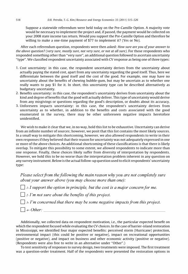
We wish to make it clear that we, in no way, hold this list to be exhaustive. Uncertainty can derivefrom an infinite number of sources; however, we posit that this list contains the most likely sources.In a small way to mitigate this shortcoming, however, we also allowed respondents to write in theirown responses if they believed that their reason for uncertainty was not adequately expressed in oneor more of the above choices. An additional shortcoming of these classifications is that there is likelyoverlap. To mitigate this possibility to some extent, we allowed respondents to indicate more thanone response. Finally, these choices likely suffer from diversity of interpretation by respondents.However, we hold this to be no worse than the interpretation problem inherent in any question onany survey instrument. Below is the actual follow-up question used to elicit respondents’ uncertaintytype:

Additionally, we collected data on respondent motivation, i.e., the particular expected benefit onwhich the respondent focused while evaluating the CV choices. In the case of barrier-island restorationin Mississippi, we identified four major expected benefits: perceived storm (Hurricane) protection,environmental impact (this could be positive or negative), impact on recreational opportunities(positive or negative), and impact on business and other economic activity (positive or negative).(Respondents were also free to write in an alternative under ‘‘Other’’.)

To test sensitivity of responses to survey design, two treatments were imposed. The first treatmentwas a question-order treatment. Half of the respondents were presented the restoration options in

D.R. Petrolia, T.-G. Kim / Resource and Energy Economics 33 (2011) 515–526518

order of smallest scale to greatest, whereas the other half were presented the opposite. Because thesurvey had three scenarios, the question-order treatment actually produces two effects: a ‘‘first’’ insequence effect, and a ‘‘preceded by a larger-scale scenario’’ effect.2 We include indicator variables foreach. The second was a variant of the ‘‘cheap talk’’ treatment, originally proposed by Cummings andTaylor (1999), and utilized subsequently by List (2001) and Lusk (2003), to address hypothetical bias.This treatment introduced language to the survey that explicitly stated the potential bias to therespondent. The present treatment differed from Cummings and Taylor in that it focused on theimpact of hypothetical bias on the respondent’s uncertainty of response rather than the responseitself. Those respondents that received the ‘‘cheap talk’’ treatment were given the following additionaltext to read just prior to beginning the referendum section:

Sometimes, people may be uncomfortable giving a simple ‘‘yes’’ or ‘‘no’’ answer to these types ofhypothetical questions. Although we want you to express your opinion, we also want you to beas comfortable as possible with your answers.Thus, we have included additional questions asking about how sure you are of each answer andthe main reasons for your answers and any concerns you may have. Additionally, you will haveanother opportunity at the end of the survey to express any remaining concerns, thoughts, oropinions you have about the questions, issues, or the survey itself. We hope that this format willallow you to express your opinion for each restoration option as completely and as comfortablyas possible.

Additionally, as a reminder, the following line was added to the end of each referendum questionfor the CT treatment:

(Remember that in the following questions you will be able to express how sure you are of youranswer as well as the main reason for your choice.)

As discussed earlier, it is claimed that respondents less familiar with the good in question should beless certain of their WTP response. As a side note, List (2001) and Lusk (2003) found that the use ofcheap talk had an effect on WTP responses, but only among respondents less knowledgeable of thegood in question. We identified two alternative measures of familiarity most relevant for this analysis:one was geographical: respondents living on the coast were expected to be more familiar with thebarrier islands; the second was experiential: respondents who have actually visited the barrier islands(irrespective of where they live) were expected to be more familiar with the barrier islands. Theseclassifications were done as follows: residents of the three coastal counties were classified as ‘‘coastalresidents’’, and the remaining as ‘‘non-coastal residents’’. The experience variable, however, was foundto be essentially interchangeable with the residence variable, and has hence not been used in theeconometric estimation.

In total, the survey instrument contained thirty-seven questions and was mailed to 3000Mississippi households on February 27, 2008, with half sent to a random sample of coastal residents(i.e., residents of Hancock, Harrison, and Jackson counties) and half sent to a random sample across theremaining 79 non-coastal counties. This oversampling of coastal residents was intentional based onthe expected low response rate from non-coastal residents, and is discussed later in the article.Reminder postcards were mailed a week later. In addition to the data discussed above, demographicdata were collected as well.

3. Data

Five-hundred ninety-four surveys were returned, for a 20% overall response rate. The low responserate may be partially explained by the fact that we sent out only a reminder postcard and not a secondsurvey, nor did we offer any incentives. It is also possible that the low response rate was a function ofthe particular population under study: Hite et al. (2002) noted at least that previous mail surveys in

2 An anonymous reviewer pointed out the fact that there are in fact two effects, not just one. We tested the model with both

the two treatment indicators and with a single question-order indicator (for each scale), and both work equally well (with

different interpretations), but we find the two-treatment approach more interesting and present that model here.

D.R. Petrolia, T.-G. Kim / Resource and Energy Economics 33 (2011) 515–526 519

Mississippi resulted in extremely low response rates. The sample was found to be biased relative to thepopulation.3 Because the purpose of this analysis is to examine methodological issues that are notnecessarily dependent on the representativeness of the sample, we do not make any attempts tomitigate sample bias.

Note that 357 respondents (61%) were classified as coastal residents and 230 (39%) were classifiedas non-coastal residents. The three coastal counties actually account for only 12% of the state’spopulation. Any significant differences in demographics across the two survey design treatments(question order and cheap talk) were tested using a Kruskal–Wallis equality of populations rank test.With the exception of age under the question-order treatment only (which was significant at the 10%probability level, and the difference in median age was 2 years), there were no significant differencesacross treatment samples. Based on these results, we proceeded assuming that the treatmentsubsamples were not biased.

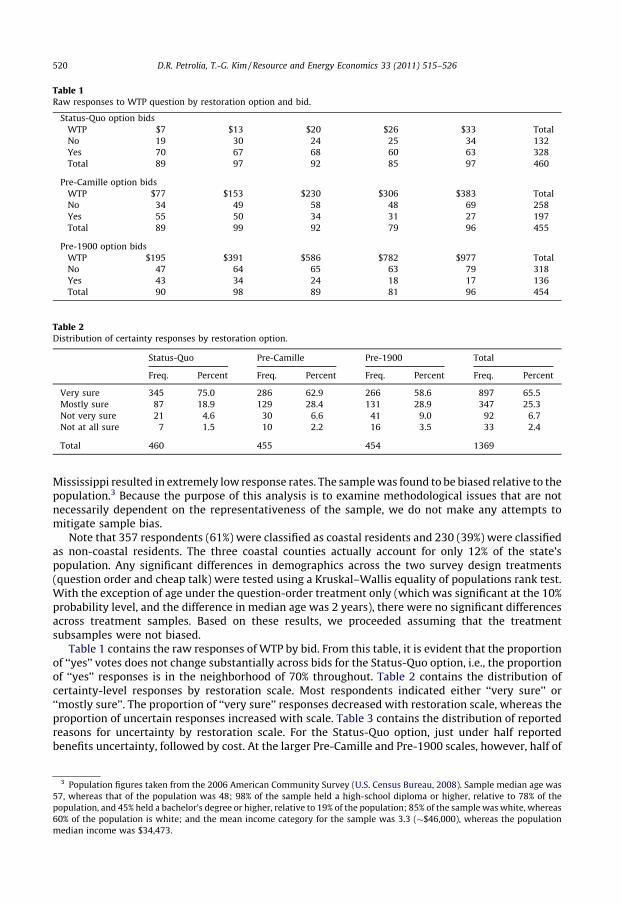
Table 1 contains the raw responses of WTP by bid. From this table, it is evident that the proportionof ‘‘yes’’ votes does not change substantially across bids for the Status-Quo option, i.e., the proportionof ‘‘yes’’ responses is in the neighborhood of 70% throughout. Table 2 contains the distribution ofcertainty-level responses by restoration scale. Most respondents indicated either ‘‘very sure’’ or‘‘mostly sure’’. The proportion of ‘‘very sure’’ responses decreased with restoration scale, whereas theproportion of uncertain responses increased with scale. Table 3 contains the distribution of reportedreasons for uncertainty by restoration scale. For the Status-Quo option, just under half reportedbenefits uncertainty, followed by cost. At the larger Pre-Camille and Pre-1900 scales, however, half of

Table 2Distribution of certainty responses by restoration option.

Status-Quo Pre-Camille Pre-1900 Total

Freq. Percent Freq. Percent Freq. Percent Freq. Percent

Very sure 345 75.0 286 62.9 266 58.6 897 65.5

Mostly sure 87 18.9 129 28.4 131 28.9 347 25.3

Not very sure 21 4.6 30 6.6 41 9.0 92 6.7

Not at all sure 7 1.5 10 2.2 16 3.5 33 2.4

Total 460 455 454 1369

Table 1Raw responses to WTP question by restoration option and bid.

Status-Quo option bids

WTP $7 $13 $20 $26 $33 Total

No 19 30 24 25 34 132

Yes 70 67 68 60 63 328

Total 89 97 92 85 97 460

Pre-Camille option bids

WTP $77 $153 $230 $306 $383 Total

No 34 49 58 48 69 258

Yes 55 50 34 31 27 197

Total 89 99 92 79 96 455

Pre-1900 option bids

WTP $195 $391 $586 $782 $977 Total

No 47 64 65 63 79 318

Yes 43 34 24 18 17 136

Total 90 98 89 81 96 454

3 Population figures taken from the 2006 American Community Survey (U.S. Census Bureau, 2008). Sample median age was

57, whereas that of the population was 48; 98% of the sample held a high-school diploma or higher, relative to 78% of the

population, and 45% held a bachelor’s degree or higher, relative to 19% of the population; 85% of the sample was white, whereas

60% of the population is white; and the mean income category for the sample was 3.3 (�$46,000), whereas the population

median income was $34,473.

D.R. Petrolia, T.-G. Kim / Resource and Energy Economics 33 (2011) 515–526520

the responses were for cost uncertainty, followed by benefits, then negative impacts and ‘‘other’’.Thus, as cost increased, uncertainty associated with cost increased as well.

4. Econometric estimation methods

Respondents were asked to consider each restoration option independently, against no action,regardless of their response to the other two options. Thus, each option could be modeledindependently as a binary-choice dependent variable, where a value of ‘‘1’’ indicates a ‘‘yes’’ vote insupport of the restoration option, and a value of ‘‘0’’ indicates a ‘‘no’’ vote. However, becauserespondents were asked to evaluate all three options in the same survey, it is likely that the errorsacross the three choices were correlated. To address this possibility, we structured the data as a paneland adopted a random-effects approach (Greene, 2000). Shaikh et al. (2007) provide a summary ofthe various ways uncertainty information has been incorporated into contingent valuation models inthe literature. In order to test the robustness of our results, we specify and estimate five differentmodels based on how the dependent variable is specified.4 The first is a random-effect probit modelwhere the dependent variable is simply the respondent’s vote, regardless of the stated certainty level.The second is a certainty-weighted random-effects probit model, where the likelihood function isweighted using respondent stated certainty level. Adapting our more-limited certainty scale to thatused by Li and Mattsson, we assigned ‘‘very sure’’ responses a weight of 1.00, ‘‘mostly sure’’, 0.75, ‘‘notvery sure’’, 0.50, and ‘‘not at all sure’’, 0.25. This model is similar to that of Li and Mattsson (1995). Thethird is an asymmetric uncertainty (ASUM) random-effects probit model, where the dependentvariable is recoded such that ‘‘yes’’ response with weak certainty levels (i.e., ‘‘not very sure’’ or ‘‘not atall sure’’) are treated as ‘‘no’’ responses. This approach is similar to that of Champ et al. (1997) andReady et al. (2001). The fourth and fifth models are symmetric uncertainty (SUM) random-effectstwo-limit tobit models, where the dependent variable is specified on a continuum from zero to oneusing vote and certainty-level data. In Model T1 (‘‘T’’ for tobit), a ‘‘very sure yes’’ is coded as a 1, a‘‘mostly sure yes’’ is 0.75, a ‘‘not very sure yes’’ is 0.625, a ‘‘not at all sure yes’’ is 0.5, a ‘‘not at all no’’ is0.5, a ‘‘not very sure no’’ is .375, a ‘‘mostly sure no’’ is 0.75, and a ‘‘very sure no’’ is coded as a zero. InModel T2, a ‘‘very sure yes’’ is coded as a 1, any other uncertain ‘‘yes’’ is coded as 0.75, any uncertain‘‘no’’ is coded as 0.25, and a ‘‘very sure no’’ is coded as a zero. These models are similar to that ofLoomis and Ekstrand (1998).

Table 4 summarizes the variables, including type, description, and mean, used in the econometricestimation. Hurricane protection and environmental impact were the two leading concerns stated byrespondents as influencing their decision-making process. Accordingly, a dummy variable wasincluded for each of these, with the remaining motives folded into the base. Additionally, a coastal-resident dummy variable was included. The Hurricane protection and coastal resident variables werehighly correlated, so an interaction term was included as well. Demographic variables include income,gender, age, and education level. Dummy variables were included to account for the threeaforementioned survey design effects.

Table 3Distribution of reasons for uncertainty by restoration optiona.

Status-Quo Pre-Camille Pre-1900 Total

Freq. Percent Freq. Percent Freq. Percent Freq. Percent

Cost 28 21.9 94 48.5 108 49.8 230 42.7

Benefits 59 46.1 57 29.4 58 26.7 174 32.3

Negative impacts 25 19.5 18 9.3 25 11.5 68 12.6

Other 16 12.5 25 12.9 26 12.0 67 12.4

Total 128 194 217 539 100.0a Because respondents could indicate more than one choice, not all observations represent individual respondents.

4 We also estimated individual models for each of the three restoration scenarios separately for each of the five model types.

We omit them here for the sake of space, but their results are consistent with the results reported in this paper.

D.R. Petrolia, T.-G. Kim / Resource and Energy Economics 33 (2011) 515–526 521

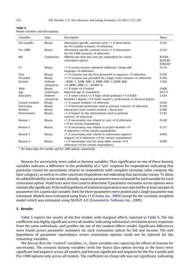
Reasons for uncertainty were coded as dummy variables. Thus significance on one of these dummyvariables indicates a difference in the probability of a ‘‘yes’’ response for respondents indicating thatparticular reason for uncertainty relative to respondents with complete certainty (who comprise thebase category), as well as to other uncertain respondents not indicating that particular reason. To allowfor added flexibility in the model, initially, separate parameters were estimated for each variable for eachrestoration option. Wald tests were then used to determine if parameter estimates across options werestatistically significant. If the null hypothesis of statistical equivalence was rejected for at least one pair ofparameters for a particular variable, then the three parameters were pooled and a single parameter wasestimated. Models were estimated using Stata 11.0 (Stata, Inc., 2009) except for the certainty-weightedmodel which was estimated using NLOGIT 4.0 (Econometric Software Inc., 2009).

5. Results

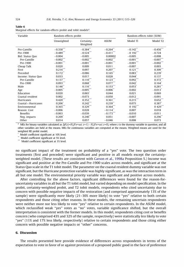
Table 5 reports the results of the five models with marginal effects reported in Table 6. The rhocoefficient was highly significant across all models, indicating substantial correlation across responsesfrom the same individuals, and justifies the use of the random-effects model. Significant differenceswere found across parameter estimates for each restoration option for bid and income. The nullhypothesis of parameter equivalence across restoration options could not be rejected for theremaining variables.

We discuss first the ‘‘control’’ variables, i.e., those variables not capturing the effects of reasons foruncertainty. The scenario dummy variables (with the Status Quo option serving as the base) weresignificant and negative across all models, and bid was significant and negative for the Pre-Camille andPre-1900 options only across all models. The coefficient on cheap talk was not significant, indicating

Table 4Model variables and descriptions.

Variables Type Description Mean

Pre-Camille Binary Alternative-specific constant term;=1 if observation

for Pre-Camille scenario;=0 otherwise

0.332

Pre-1900 Binary Alternative-specific constant term;=1 if observation

for Pre-1900 scenario;=0 otherwise

0.332

Bid Continuous Offered one-time bid (cost per respondent for stated

restoration option)

$19.86,

$228.80,

$584.04a

CT Binary =1 if survey version contained additional ‘cheap talk’

language;=0 otherwise

0.519

First Binary =1 if scenario was the first presented in sequence;=0 otherwise 0.338

Preceded Binary =1 if scenario was preceded by a larger-scale scenario;=0 otherwise 0.305

Income Ordered

categorical

<$20K=1, $20K–40K=2, $40K–60K=3, $60K–80K

=4, $80K–100K=5, >$100K=6

3.394

Male Binary =1 if male;=0 if female 0.606

Age Continuous Reported age of respondent 56.571

Education Ordered

categorical

=1 if some school;=2 if high school graduate;=3 if holds

bachelor’s degree;=4 if holds master’s, professional, or doctoral degree

2.634

Coastal resident Binary =1 if coastal resident;=0 otherwise 0.620

Hurricanes Binary =1 if Hurricane protection cited as primary concern;=0 otherwise 0.526

ResHurr Binary Interaction term: coastal resident�Hurricanes 0.346

Environment Binary =1 if impact on the environment cited as primary

concern;=0 otherwise

0.183

Reason 1 Binary =1 if uncertainty was related to cost;=0 if otherwise

(=0 for certain respondents)

0.168

Reason 2 Binary =1 if uncertainty was related to project benefits;=0

if otherwise (=0 for certain respondents)

0.127

Reason 3 Binary =1 if uncertainty was related to unforeseen negative

impacts;=0 if otherwise (=0 for certain respondents)

0.050

Reason 4 Binary =1 if uncertainty was for some other reason;=0 if

otherwise (=0 for certain respondents)

0.049

a For Status-Quo, Pre-Camille, and Pre-1900 options, respectively.

D.R. Petrolia, T.-G. Kim / Resource and Energy Economics 33 (2011) 515–526522

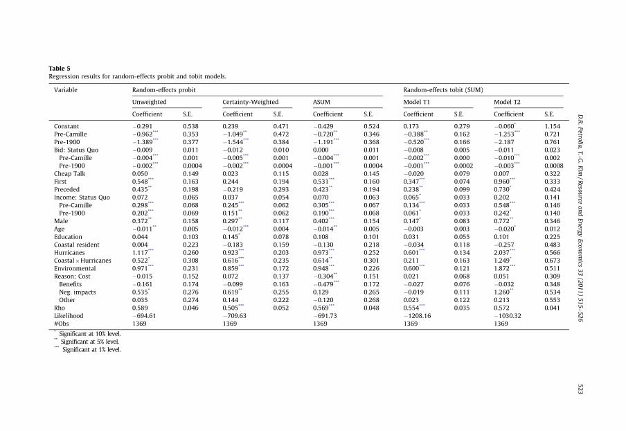
Table 5Regression results for random-effects probit and tobit models.

Variable Random-effects probit Random-effects tobit (SUM)

Unweighted Certainty-Weighted ASUM Model T1 Model T2

Coefficient S.E. Coefficient S.E. Coefficient S.E. Coefficient S.E. Coefficient S.E.

Constant �0.291 0.538 0.239 0.471 �0.429 0.524 0.173 0.279 �0.060* 1.154

Pre-Camille �0.962*** 0.353 �1.049** 0.472 �0.720** 0.346 �0.388** 0.162 �1.253*** 0.721

Pre-1900 �1.389*** 0.377 �1.544*** 0.384 �1.191*** 0.368 �0.520*** 0.166 �2.187 0.761

Bid: Status Quo �0.009 0.011 �0.012 0.010 0.000 0.011 �0.008 0.005 �0.011 0.023

Pre-Camille �0.004*** 0.001 �0.005*** 0.001 �0.004*** 0.001 �0.002*** 0.000 �0.010*** 0.002

Pre-1900 �0.002*** 0.0004 �0.002*** 0.0004 �0.001*** 0.0004 �0.001*** 0.0002 �0.003*** 0.0008

Cheap Talk 0.050 0.149 0.023 0.115 0.028 0.145 �0.020 0.079 0.007 0.322

First 0.548*** 0.163 0.244 0.194 0.531*** 0.160 0.347*** 0.074 0.960*** 0.333

Preceded 0.435** 0.198 �0.219 0.293 0.423** 0.194 0.238** 0.099 0.730* 0.424

Income: Status Quo 0.072 0.065 0.037 0.054 0.070 0.063 0.065* 0.033 0.202 0.141

Pre-Camille 0.298*** 0.068 0.245*** 0.062 0.305*** 0.067 0.134*** 0.033 0.548*** 0.146

Pre-1900 0.202*** 0.069 0.151** 0.062 0.190*** 0.068 0.061* 0.033 0.242* 0.140

Male 0.372** 0.158 0.297** 0.117 0.402*** 0.154 0.147* 0.083 0.772** 0.346

Age �0.011** 0.005 �0.012*** 0.004 �0.014** 0.005 �0.003 0.003 �0.020* 0.012

Education 0.044 0.103 0.145* 0.078 0.108 0.101 0.031 0.055 0.101 0.225

Coastal resident 0.004 0.223 �0.183 0.159 �0.130 0.218 �0.034 0.118 �0.257 0.483

Hurricanes 1.117*** 0.260 0.923*** 0.203 0.973*** 0.252 0.601*** 0.134 2.037*** 0.566

Coastal�Hurricanes 0.522* 0.308 0.616*** 0.235 0.614** 0.301 0.211 0.163 1.249* 0.673

Environmental 0.971*** 0.231 0.859*** 0.172 0.948*** 0.226 0.600*** 0.121 1.872*** 0.511

Reason: Cost �0.015 0.152 0.072 0.137 �0.304** 0.151 0.021 0.068 0.051 0.309

Benefits �0.161 0.174 �0.099 0.163 �0.479*** 0.172 �0.027 0.076 �0.032 0.348

Neg. impacts 0.535* 0.276 0.619** 0.255 0.129 0.265 �0.019 0.111 1.260** 0.534

Other 0.035 0.274 0.144 0.222 �0.120 0.268 0.023 0.122 0.213 0.553

Rho 0.589 0.046 0.505*** 0.052 0.569*** 0.048 0.554*** 0.035 0.572 0.041

Likelihood �694.61 �709.63 �691.73 �1208.16 �1030.32

#Obs 1369 1369 1369 1369 1369* Significant at 10% level.** Significant at 5% level.*** Significant at 1% level.

D.R

.P

etrolia

,T

.-G.

Kim

/Reso

urce

an

dE

nerg

yE

con

om

ics3

3(2

01

1)

51

5–

52

65

23

no significant impact of the treatment on probability of a ‘‘yes’’ vote. The two question ordertreatments (first and preceded) were significant and positive in all models except the certainty-weighted model. (These results are consistent with Carson et al., 1998a Proposition 5.) Income wassignificant and positive at the Pre-Camille and Pre-1900 scales across models, and significant at theStatus Quo scale in the T1 tobit model. The parameter on the coastal resident dummy variable was notsignificant, but the Hurricane protection variable was highly significant, as was the interaction term inall but one model. The environmental priority variable was significant and positive across models.

After controlling for the above factors, significant differences were found for the reason-for-uncertainty variables in all but the T1 tobit model, but varied depending on model specification. In theprobit, certainty-weighted probit, and T2 tobit models, respondents who cited uncertainty due toconcern with possible negative impacts of the restoration (and comprised approximately 13% of thesample) were significantly more likely (21–30% more likely) to vote ‘‘yes’’ relative to both certainrespondents and those citing other reasons. In these models, the remaining uncertain respondentswere neither more nor less likely to vote ‘‘yes’’ relative to certain respondents. In the ASUM model,which reclassified weak ‘‘yes’’ votes as ‘‘no’’ votes, variable significance shifted, but the overallinterpretation is consistent with the former models. In this model, respondents citing cost or benefitsconcern (who comprised 43% and 32% of the sample, respectively) were statistically less likely to vote‘‘yes’’ (11% and 17% less likely, respectively) relative to certain respondents and those citing eitherconcern with possible negative impacts or ‘‘other’’ concerns.

6. Discussion

The results presented here provide evidence of differences across respondents in terms of theexpectation to vote in favor of or against provision of a proposed public good in the face of preference

Table 6Marginal effects for random-effects probit and tobit modelsa.

Variable Random-effects probit Random-effects tobit (SUM)

Unweighted Certainty-

Weighted

ASUM Model Tl Model T2

Pre-Camille �0.358*** �0.384** �0.264** �0.142** �0.456***

Pre-1900 �0.489*** �0.524*** �0.411*** �0 192*** �0.724

Bid: Status Quo �0.004 �0.005 0.00002 �0.005 �0.008

Pre-Camille �0.002*** �0.002*** �0.002*** �0.001*** �0.007***

Pre-1900 �0.001*** �0.001*** �0.001*** �0.001*** �0.002***

Cheap Talk 0.020 0.009 0.011 �0.007 0.003

First 0.216*** 0.097 0.207*** 0.121*** 0.309***

Preceded 0.172** �0.086 0.165** 0.083** 0.239*

Income: Status Quo 0.033 0.017 0.028 0.044* 0.137

Pre-Camille 0.137*** 0.110*** 0.123*** 0.092*** 0.372***

Pre-1900 0.093*** 0.068** 0.077*** 0.042* 0.164*

Male 0.146** 0.116** 0.153*** 0.053* 0.281**

Age �0.005** �0.005*** �0.006** �0.002 �0.013*

Education 0.020 0.065* 0.044 0.021 0.069

Coastal resident 0.002 �0.073 �0.050 �0.012 �0.091

Hurricanes 0.420*** 0.352*** 0.361*** 0.215*** 0.652***

Coastal�Hurricanes 0.206* 0.242*** 0.239** 0.075 0.387*

Environmental 0.365*** 0.329*** 0.364*** 0 192*** 0 429***

Reason: Cost �0.006 0.028 �0.114** 0.007 0.018

Benefits �0.063 �0.039 �0.173*** �0.010 �0.011

Neg. impacts 0.209* 0.240** 0.051 �0.007 0.296**

Other 0.014 0.057 �0.046 0.008 0.073a MEs for binary variables calculated as DF(z)=F((b0x+azj z=1)�F((b0x+azj z=0), where z is the dummy variable in question, and all

other variables are held at the means. MEs for continuous variables are computed at the means. Weighted means are used for the

weighted RE probit model.* Model coefficient significant at 10% level.** Model coefficient significant at 5% level.*** Model coefficient significant at 1% level.

D.R. Petrolia, T.-G. Kim / Resource and Energy Economics 33 (2011) 515–526524

uncertainty. Three of the five model presented indicate that respondents whose uncertainty derivesfrom concern about unexpected negative impacts from provision of the good were more likely to vote‘‘yes’’ relative to both certain respondents and respondents who are uncertain for other reasons. Onthe other hand, one of the models indicates that those whose uncertainty derives from cost (i.e., theprice and its impact on their budget, apart from the marginal effect of income itself, captured by theincome variable) and those whose uncertainty derives from doubts about the expected benefits of thegood were more likely to vote ‘‘no’’ relative to all others.

Although the latter result is not supported by the other models, it does not contradict them.Although the former three models indicate a significant positive difference for respondents citing‘‘negative impacts’’ and the latter model indicates a significant negative difference for respondentsciting ‘‘cost’’ and ‘‘benefit’’, the overall interpretation of the results is that these groups of uncertainrespondents tended to vote consistently in opposite directions. When those citing cost or benefitconcerns were found to be equally likely to vote ‘‘yes’’ as certain respondents (as in three of the fivemodels), those citing possible negative impacts were more likely to vote ‘‘yes’’; similarly, when thoseciting possible negative impacts were found to be equally likely to vote ‘‘yes’’ as certain respondents(as in the ASUM model), those citing cost or benefit concerns were less likely to vote ‘‘yes’’.

How can these results be interpreted? Cost and benefits were directly and explicitly detailed in thesurvey, and thus the impact of these on respondent utility is clearer. On the other hand, the potentialnegative impacts of provision of the good are vague. Negative impacts of provision were not explicitlystated in the scenarios; thus the negative impacts conceived of by the respondent, whatever they maybe, are their own. Additionally, the probabilities of realizing such negative impacts assigned by eachrespondent are their own, and may be low. This would, at least, help explain the tendency to vote ‘‘yes’’under this kind of uncertainty. Some anecdotal evidence is that several respondents indicated thenegative impact of the payment on poor residents of the state; i.e., they indicated their own personalsupport for the project and their own personal ability to pay for it, but they were concerned that otherswould not have the means to do so. Anyway, there is some evidence to point to the conclusion thatuncertainty deriving from concerns more remote to the respondent, however such remoteness maketake form, the more likely to vote in favor when uncertain.

We would like to make a few modest comparisons to previous findings. Welsh and Poe (1998)and Flachaire and Hollard (2007) concluded that uncertain respondents tend to vote ‘‘yes’’. Such aconclusion would be consistent with the findings for our uncertain respondents concerned withnegative impacts, although they comprised just 13% of the total responses given. Not differentiatingby reason would mask such a finding if the dominant reasons for uncertainty tended to result in‘‘no’’ responses. Carson et al. (1998b) concluded that uncertain respondents tend to vote ‘‘no’’. Thisfinding would correspond to our uncertain respondents concerned with cost and/or projectbenefits. If respondents with differing reasons for uncertainty were fairly equally distributed(which was not the case here), then the result may be consistent with the two interpretations putforth by Carson et al. (1998b), that uncertainty derives from the ‘‘yes’’ and ‘‘no’’ voting groupsproportionally.

It is at least possible to hypothesize that the composition of uncertain respondents in any givensurvey differs. For one, the dominant reason for uncertainty may be cost, and in another, benefitsuncertainty, leading uncertain respondents to vote ‘‘no’’, whereas in another the dominant reason maybe possible negative impacts, leading uncertain respondents to vote ‘‘yes’’. We offer our results simplyas some evidence that reason for uncertainty may be one possible avenue to better differentiateuncertain respondents and thus better account for such respondents in our CV models.

Obvious shortcomings of the results here are (1) that these distinctions hold for the specific goodbeing valued here only; (2) that contrary results could be had if the uncertainty categories were re-defined or if additional categories were offered; and (3) that these reasons for uncertainty may be justproxies for the true reasons for uncertainty, and the true reasons may not actually be concern withcost, benefits, etc., but with something else. Further testing of these categories on additional scenarios,and further vetting of the categories themselves is clearly warranted and the subject of furtherresearch. This work represents merely a first swipe at better understanding the voting tendencies ofrespondents with uncertain preferences by way of better understanding the reasons why it is that theyare uncertain.

D.R. Petrolia, T.-G. Kim / Resource and Energy Economics 33 (2011) 515–526 525

Acknowledgements

This research was conducted under award NA06OAR4320264 06111039 to the Northern GulfInstitute by the NOAA Office of Ocean and Atmospheric Research, U.S. Department of Commerce, andby the USDA Cooperative State Research, Education & Extension Service, Hatch project MIS-012030,‘‘Valuation of Environmental Goods and Natural Resources’’.

References

Alberini, A., Boyle, K., Welsh, M., 2003. Analysis of contingent valuation data with multiple bids and response options allowingrespondents to express uncertainty. Journal of Environmental Economics and Management 45, 40–62.

Arrow, K., Solow, R., Portney, P.R., Leamer, E.E., Radner, R., Schuman, H., 1993. Report of the NOAA panel on contingent valuation.Federal Register 58, 4601–4614.

Broberg, T., Brannlund, R., 2008. An alternative interpretation of multiple bounded WTP data—certainty dependent paymentcard intervals. Resource and Energy Economics 30, 555–567.

Carson, R., Flores, N.E., Hanemann, W.M., 1998a. Sequencing and valuing public goods. Journal of Environmental Economics andManagement 36, 314–323.

Carson, R.T., Hanemann, W.M., Kopp, R.J., Krosnick, J.A., Mitchell, R.C., Presser, S., Ruud, P.A., Smith, V.K., Conaway, M., Martin, K.,1998b. Referendum design and contingent valuation: the NOAA panel’s no-vote recommendation. The Review of Economicsand Statistics 80, 484–487.

Carter, G.A., Blossom, G., 2007. Unpublished Maps. Gulf Coast Geospatial Center, University of Southern Mississippi.Champ, P.A., Bishop, R.C., Brown, T.C., McCollum, D.W., 1997. Using donation mechanisms to value nonuse benefits from public

goods. Journal of Environmental Economics and Management 33, 151–162.Cummings, R.G., Taylor, L.O., 1999. Unbiased value estimates for environmental goods: a cheap talk design for the contingent

valuation method. The American Economic Review 89, 649–665.Econometric Software, Inc., 2009. NLOGIT 4.0.Flachaire, E., Hollard, G., 2007. Starting point bias and respondent uncertainty in dichotomous choice contingent valuation

surveys. Resource and Energy Economics 29, 183–194.Greene, W.H., 2000. Econometric Analysis, 4th ed. Prentice-Hall, Inc., Upper Saddle River, NJ.Hite, D., Hudson, D., Intarapapong, W., 2002. Willingness to pay for water quality improvements: the case for precision

application technology. Journal of Agricultural and Resource Economics 27, 433–449.Li, C., Mattsson, L., 1995. Discrete choice under preference uncertainty: an improved structural model for contingent valuation.

Journal of Environmental Economics and Management 28, 256–269.List, J.A., 2001. Do explicit warnings eliminate the hypothetical bias in elicitation procedures? Evidence from field auctions for

sportscards. American Economic Review 91, 1498–1507.Loomis, J., Ekstrand, E., 1998. Alternative approaches for incorporating respondent uncertainty when estimating willingness to

pay: the case of the Mexican spotted owl. Ecological Economics 27, 29–41.Lusk, J.L., 2003. Effects of cheap talk on consumer willingness-to-pay for golden rice. American Journal of Agricultural

Economics 85, 840–856.Morton, R.A., 2007. Historic Changes in the Mississippi–Alabama Barrier Islands and the Roles of Extreme Storms, Sea Level, and

Human Activities. US Geological Survey, Coastal and Marine Geology Program, Open-File Report 2007-1161.Ready, R.C., Navrud, S., Dubourg, W.R., 2001. How do respondents with uncertain willingness to pay answer contingent

valuation questions? Land Economics 77, 315–326.Shaikh, S.L., Sun, L., van Kooten, G.C., 2007. Treating respondent uncertainty in contingent valuation: a comparison of empirical

treatments. Ecological Economics 62, 115–125.Stata Corporation, Inc., 2009. Stata 11.0.T. Baker Smith & Sons, Inc., 1997. Barrier Island Plan, Phase 1—Step K Report: Identification and Assessment of Management and

Engineering Techniques, Louisiana Dept. of Natural Resources Contract No. 25081-95-02.U.S. Census Bureau, 2008. 2006 American Community Survey. http://factfinder.census.gov/servlet/ACSSAFFFacts?_event=Sear-

ch&_lang=en&_sse=on&geo_id=04000US28&_state=04000US28, last accessed October 3, 2008.Wang, H., 1997. Treatment of ‘‘don’t know’’ responses in contingent valuation surveys: a random valuation model. Journal of

Environmental Economics and Management 32, 219–232.Welsh, M.P., Poe, G.L., 1998. Elicitation effects in contingent valuation: comparisons to a multiple bounded discrete choice

approach. Journal of Environmental Economics and Management 36, 170–185.

D.R. Petrolia, T.-G. Kim / Resource and Energy Economics 33 (2011) 515–526526