Applying the Contingent Valuation Method in Resource Accounting: A Bold Proposal Mattias Boman, Anni Huhtala, Charlotte Nilsson, Sofia Ahlroth, Göran Bostedt, Leif Mattson, Peichen Gong

Working Paper No. 85, June 2003 Published by The National Institute of Economic Research Stockholm 2003

NIER prepares analyses and forecasts of the Swedish and international economy and conducts related research. NIER is a government agency accountable to the Ministry of Finance and is financed largely by Swedish government funds. Like other government agencies, NIER has an independent status and is responsible for the assessments that it publishes. The Working Paper series consists of publications of research reports and other detailed analyses. The reports may concern macroeconomic issues related to the forecasts of the Institute, research in environmental economics in connection with the work on environmental accounting, or problems of economic and statistical methods. Some of these reports are published in final form in this series, whereas others are previous versions of articles that are subsequently published in international scholarly journals under the heading of Reprints. Reports in both of these series can be ordered free of charge. Most publications can also be downloaded directly from the NIER home page. NIER Kungsgatan 12-14 Box 3116 SE-103 62 Stockholm Sweden Phone: 46-8-453 59 00, Fax: 46-8-453 59 80 E-mail: ki@konj.se, Home page: www.konj.se ISSN 1100-7818

Applying the Contingent Valuation Method in Resource Accounting:

A Bold Proposal

Mattias Boman1, Anni Huhtala2, Charlotte Nilsson3, Sofia Ahlroth4, Göran Bostedt5, Leif

Mattsson1, Peichen Gong5

Abstract

Resource accounting involves complementing conventional national accounts with changes in

environmental and natural resource capital valued in monetary terms. By adopting the

Ramsey device of “Bliss”, we derive a theoretically consistent environmentally adjusted NDP

(Net Domestic Product) measure. The measure indicates sustainable future consumption that

an economy can support along the optimal path approaching “Bliss”, or “sustainability”

determined by national environmental goals. The goals accepted by the Swedish parliament

are used to show the applicability of the contingent valuation method to elicit non-market

benefits of an economy approaching the sustainability targets. We investigate the

compatibility of marginal willingness to pay measures derived on hypothetical markets with

market prices used in national accounts. Finally, we raise certain issues of survey design, e.g.

to take advantage of the CVM as a democratic device for value estimation over time.

Keywords: Sustainability goals, Ramsey device, Contingent valuation, Environmental

budget, Marginal willingness to pay, Survey design.

JEL Classification:

D60 (Welfare economics, general)

O4 (Economic growth and aggregate productivity)

Q26 (Contingent valuation)

1 Southern Swedish Forest Research Centre, Swedish University of Agricultural Sciences, Box 49, SE-230 53 Alnarp, Sweden. 2 Environmental Economics, MTT Economic Research, Luutnantintie 13, FI-00410 Helsinki, Finland. 3 National Institute of Economic Research, Box 3116, SE-103 62 Stockholm, Sweden. 4 Environmental Strategies Research Group, Box 2142, SE-103 14 Stockholm, Sweden. 5 Dept. of Forest Economics, Swedish University of Agricultural Sciences, SE-901 83 Umeå, Sweden.

2

1. Introduction

Social accounting attempts to augment the national accounts to obtain an indicator of the

nation's economic performance that could be an alternative to the traditional GDP (gross

domestic product) measure. The motivation is that GDP is often misinterpreted as a measure

of societal welfare. An important part of extending the existing national income and product

accounts framework is to integrate environmental aspects into the economic accounts. Hence,

the integrated accounts would also provide information about how the economy performs

from an environmental point of view and how the economic and environmental policy

adopted (green taxes, regulations) affects welfare over time. Quantifiable environmental data

would then be comparable to other policy decisions. The interest in monetary environmental

accounts is also explained by the fact that many countries consider using economic

instruments to a larger extent than before to co-ordinate national and international energy and

environmental policy.

In 1993, the London Group on Environmental Accounting was created to provide an informed

forum for practitioners to share their experience of developing and implementing

environmental satellite accounts linked to the economic accounts of the System of National

Accounts (SNA, 1993). A result of this work is the handbook Integrated Environmental and

Economic Accounts, “SEEA 2003”, currently in press. In principle, SEEA 2003 gives a

framework for monetary environmental satellite accounts, linked to the SNA. However, the

current experience in large-scale valuation exercises and calculations of environmentally

adjusted national account aggregates is very limited. It seems evident that an aggregate such

as a “green” Net Domestic Product (NDP) cannot be the ultimate goal of compiling

environmental accounts. More specifically, the following excerpt from SEEA 2003, (ch.10,

para 10.254) reflects the prevalent consensus among accounting practitioners: “… economic

aggregates from the SEEA will be necessarily less precise than those coming from the SNA.

Collaboration with users as new versions of the accounts are developed is important to allow

external review of the techniques adopted and the quality of the results and also to avoid

raising unrealistic expectations among users.”

The SEEA handbook discusses alternative methods of valuing environmental degradation, i.e.

decline in resource quality rather than quantity, specifically air and water quality. One of the

potential monetary valuation methods mentioned is the Contingent Valuation Method (CVM,

cf. Mitchell and Carson, 1989 or Bjornstad and Kahn, 1996), which has now been in use for

3

more than 35 years, and more than 2000 papers can be found on this topic (Carson, 2000). In

terms of number of publications, CVM is currently the dominating method for nonmarket

valuation.

Nevertheless, there is no established agenda for the application of CVM in a green accounting

context.The SEEA 2003 handbook states that: “The possibilities of incorporating adjustments

for depletion and defensive expenditure into the flow accounts [using market prices, our note] are

much more promising for a statistical office at this time though even here there may be

reservations about proceeding with the work on theoretical or practical grounds. By contrast, it

seems that work on degradation will stay mainly in research field for some time” (SEEA 2003,

ch.10. para 10.251). Accordingly, it is important to acknowledge the very experimental nature

of the suggested application, and that it is only one part of a larger picture of physical and

environmental economic accounting. Bearing this reservation in mind, the following

requirements for satellite accounts with environmental valuation are crucial for our exercise:

- consistency with accounting principles in terms of valuation methods used and in terms of

accounting periods (one year) and coverage (economic territory, domestic economy),

- consistency as far as possible with economic theory or theories,

- availability of the basic data,

- relevance of the results for decision making,

- appropriateness of the results for the environmental issues covered, and

- comprehensiveness in coverage of phenomena and values.

To meet these requirements by using CVM for valuation of environmental effects is not a

trivial issue. There are several critical factors associated with contingent valuation in the

national accounting context. First, a typical welfare measure derived from CVM studies is a

Hicksian consumer surplus measure. However, including these welfare measures as such in

environmental satellite accounts would not be consistent with the national accounts that use

equilibrium market prices in valuation. Therefore, one should aim at deriving a marginal

willingness to pay measure per given emission/environmental unit valued. Second, in national

environmental accounts large-scale, multiple goods valuation is required instead of a single

product/project valuation. There are at least two potential problems with multiple valuation:

sequencing of valuation of environmental goods, and the overall budget constraint for

consumption of private goods and environmental commodities. Third, the microeconomic

4

foundations of CVM and green accounting based on welfare theory should be merged in a

consistent manner. Finally, an important issue is the comparability of the derived values over

time. We discuss and present potential solutions for overcoming these problems. A resulting

set of CVM data would then have the following characteristics:

a) a marginal valuation of avoiding environmental degradation,

b) a disaggregation into a vector of marginal values for different types of environmental

degradation, and

c) repeated and intertemporally consistent estimates of a) and b).

The purpose of this paper is to derive a theoretical and methodological approach that is

amenable to these data requirements.

Standardized guidelines for CVM applications in general were set out by the NOAA (1993)

panel. Most of these guidelines apply to a resource accounting application as well. However,

in the years that have passed since the work of NOAA, much progress has been made in the

field of CVM. In the following sections, we will review the welfare economic basis for

contingent value estimation, as well as relevant theoretical and methodological developments.

In addition, we will try to meet the challenge to match CVM with the welfare economic

analysis of green accounting developed during the recent years. The theoretical foundations of

this type of ‘extended’ welfare accounting have been actively discussed in the academic green

accounting literature, by e.g., Weitzman (1976), Solow (1986), Hartwick (1990), Mäler

(1991), Dasgupta et al. (1994), Asheim (1997), and Aronsson and Löfgren (1999).

The paper is structured as follows. Section 2 presents a theoretical framework for

comprehensive national accounting that is applied in the empirical valuation experiment. With

the help of the dynamic model, it is shown that environmentally adjusted NDP is a welfare

index for sustainable future consumption. Section 3 addresses welfare theoretical foundations

of contingent valuation. A measure of a representative consumer’s marginal willingness to

pay for an environmental good, comparable with market prices used in the national accounts,

is derived. Section 4 discusses policy relevant environmental objects to be used in an

empirical CVM application, survey design and certain methodological issues. Section 5

contains a discussion and concluding remarks.

5

2. The Resource Accounting Framework for the CVM Application

Comprehensive resource accounting should involve estimation of a value for production of

environmental goods during an accounting period (normally a year). We therefore need a

theoretical framework for carrying out the environmental accounting in a consistent way. Our

approach follows the logic presented initially in Weitzman (1976), followed by Hartwick

(1990) and Mäler (1991). The purpose of building a dynamic, optimal control model is to

have a transparent framework which gives guidelines for separating different kinds of

externalities (flows/stocks) to treat them in a correct way in annual accounts. Double counting

is another concern, which can also be avoided if monetary environmental adjustments are

based on a consistent model.

The whole accounting system relies upon the utility function, which has some specific

features and components that are worth commenting. We start out from the assumption that

society has decided on certain environmental goals that should be reached within a specified

time frame. Moreover, we assume that these goals can be quantified in terms of various

pollutants and the level of biodiversity in a country. These assumptions will be given an

empirical motivation in section 4. From the point of view of the present analysis, such environmental goals can be viewed as a type of quantity index for environmental quality.

Consequently, an individual consumer should arrive at the same solution irrespective of

whether the utility maximization problem is solved with respect to the vector of all

environmental problems in a country, or with respect to the environmental goals as an index

good. We may think of such an aggregation as a two-stage budgeting process, where the

consumption decision is first made with respect to the total environmental quality in a

country, and then with respect to the subcomponents of total environmental quality. This is

the case if the overall utility function is weakly separable and the subutility functions are

homothetic. Homothetic preferences are also sufficient for aggregating demands in the sense

of the representative consumer model (Varian, 1992; Boadway and Bruce, 1993).

We further hypothesize that the subcomponents of the overall utility function are selected to

be independent in consumption, implying that the overall utility function is additively

separable (Hoehn, 1991). A necessary and sufficient condition for additive (i.e. strong)

separability is that the marginal rate of substitution between two goods, contained in two

different subutility groups, is independent of the quantity of any other good contained in any

other group than the two under consideration (Boadway and Bruce, 1993). Hoehn (1991)

6

shows that environmental goods that are additively separable in utility are substitutes in

valuation.i This occurs e.g. when consumption is spatially separated. For the whole economy,

let us denote the utility of consumption, C, by U(C), disutility function for the vector of

emissions and concentration of pollutants, E, by α(E), the utility function for preservation of

biodiversity, P, by β(P), and the utility function for the composite vector of remaining (not

including pollutants and biodiversity) environmental and natural resource goods and services

by ))(( tv −R . The set of all environmental goal objects is implicitly defined as { }P,, ERR -= .

The separability assumption then implies that e.g. the utility of biodiversity is unaffected by

changes in the disutility of emissions and vice versa.

Another issue regarding our utility function is that we assume that the economy approaches

indefinitely the sustainability goals approved by the government. Accordingly, to formulate

our objective function we adopt the Ramsey device of “…the maximum obtainable rate of

enjoyment or utility…”, or “Bliss” (Ramsey, 1928, p. 545), denoted B . Thus,

))](())(())(())(([ tPtttCUB βαν −+−− − ER represents the amount by which utility falls

short of Bliss or sustainability, and this should be minimized. To formulate our problem as

maximization of utility, which is integrated throughout time, we write

∫∞

− −+−+0

max ]))(())(())(())(([ dtBtPtttCU βαν ER

subject to )())(())(()())(),(( tKtPgthtCttKfK δ−−−−= −⋅

RE

0)0( KK =

))(),(()(0 ttKftC E≤≤

where E = emission/concentration of pollutants (tons or micrograms/m3)

P = land area reserved for biodiversity purposes (hectares); crowds out

investments in man-made capital, g(P)

=−R composite vector containing the complement set of environmental and

natural resource goods and services, not including E and P; crowds out

investments in man-made capital, h(R-)

δ = depreciation rate of capital stock

K = stock of man-made capital

K0 = initial level of capital (given)

7

and UC>0, -Rν >0, αE>0, βP>0, fK >0, fE>0, -Rh >0, gP >0

The production factor E, emissions, could be interpreted in terms of the use of energy and

other emission-generating substances. The generated emissions contribute to the

concentration of pollution in different media (air, soil, water) in various degrees, dependent

on the pollutant and the media. For simplicity, the specific links between emissions and

concentrations are disregarded.

The current value Hamiltonian is

)]())(())(()())(),(()[())(())(())(())(()(

tKtPgthtCttKftBtPtttCUtHδλ

βαν

−−−−+

+−+−+=−

−

REER

(1)

We derive the necessary conditions for the optimization of this problem to interpret the

marginal utility of consumption with respect to the environmental goods.

∂H(t)/∂C(t)=UC - λ(t) = 0 (2)

∂H(t)/∂R-(t)=ν R- - λ(t)hR- =0 (3)

∂H(t)/∂E(t)=-αE + λ(t)fE = 0 (4)

∂H(t)/∂P(t)=β P - λ(t)gP= 0 (5)

))(())(()( kk ftftt −=−−= δλδλλ& (6)

ktktˆ)(lim =∞→ (7)

Hence, the marginal utility of consumption, UC, equals the shadow price of capital, λ(t). In

addition, the marginal disutility of emissions, αE/fE, the marginal utility of preserving an

additional unit of biodiversity, βP/gP, and the marginal utility of preserving an additional unit

of composite environmental and natural resource goods and services, ν R-/hR-, must equal the

marginal utility of consumption.

By linearizing the Hamiltonian (suppressing t) and dividing through by the marginal utility of

consumption, UC, we have

8

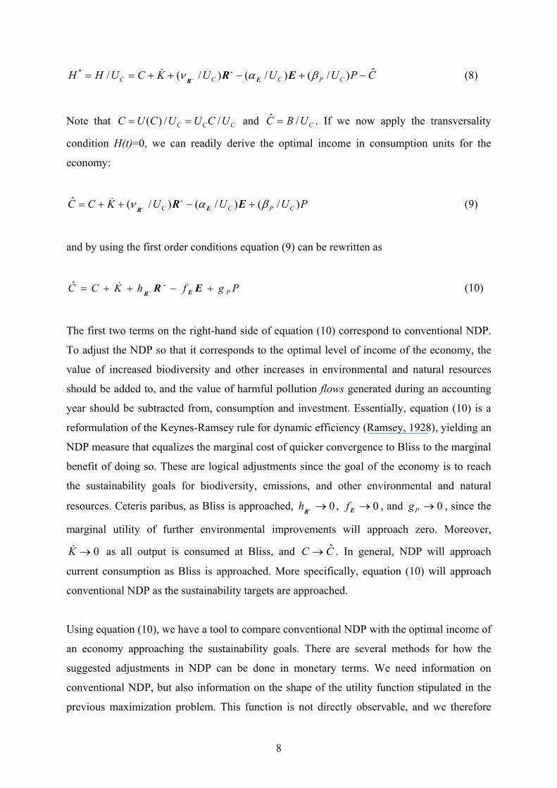
CPUUUKCUHH CPCCCˆ)/()/()/(/* −+−++== − βαν ER E

-R

& (8)

Note that CCC UCUUCUC //)( == and CUBC /ˆ = . If we now apply the transversality

condition H(t)=0, we can readily derive the optimal income in consumption units for the

economy:

PUUUKCC CPCC )/()/()/(ˆ βαν +−++= − ER E-

R& (9)

and by using the first order conditions equation (9) can be rewritten as

PgfhKCC P+−++= ER E-

R -&ˆ (10)

The first two terms on the right-hand side of equation (10) correspond to conventional NDP.

To adjust the NDP so that it corresponds to the optimal level of income of the economy, the

value of increased biodiversity and other increases in environmental and natural resources

should be added to, and the value of harmful pollution flows generated during an accounting

year should be subtracted from, consumption and investment. Essentially, equation (10) is a

reformulation of the Keynes-Ramsey rule for dynamic efficiency (Ramsey, 1928), yielding an

NDP measure that equalizes the marginal cost of quicker convergence to Bliss to the marginal

benefit of doing so. These are logical adjustments since the goal of the economy is to reach

the sustainability goals for biodiversity, emissions, and other environmental and natural

resources. Ceteris paribus, as Bliss is approached, 0→-Rh , 0→Ef , and 0→Pg , since the

marginal utility of further environmental improvements will approach zero. Moreover,

0→K& as all output is consumed at Bliss, and CC ˆ→ . In general, NDP will approach

current consumption as Bliss is approached. More specifically, equation (10) will approach

conventional NDP as the sustainability targets are approached.

Using equation (10), we have a tool to compare conventional NDP with the optimal income of

an economy approaching the sustainability goals. There are several methods for how the

suggested adjustments in NDP can be done in monetary terms. We need information on

conventional NDP, but also information on the shape of the utility function stipulated in the

previous maximization problem. This function is not directly observable, and we therefore

9

need a money measure to evaluate the marginal changes in utility given by equation (10).

Since we use the contingent valuation method we in fact derive estimates of marginal

willingness to pay (MWTP) for approaching the sustainability goals for the state of the

environment. In the next section, we show how a representative consumer maximizes utility

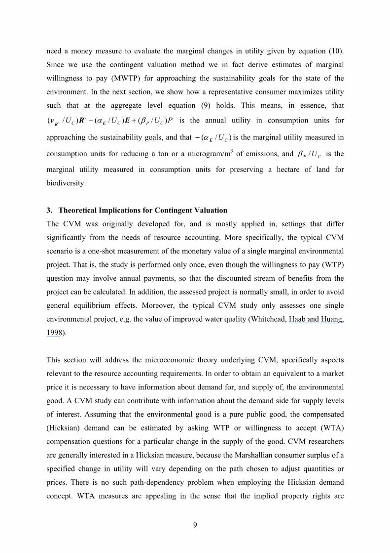
such that at the aggregate level equation (9) holds. This means, in essence, that

PUUU CPCC )/()/()/( βαν +−− ER E-

R is the annual utility in consumption units for

approaching the sustainability goals, and that )/( CUEα− is the marginal utility measured in

consumption units for reducing a ton or a microgram/m3 of emissions, and CP U/β is the

marginal utility measured in consumption units for preserving a hectare of land for

biodiversity.

3. Theoretical Implications for Contingent Valuation

The CVM was originally developed for, and is mostly applied in, settings that differ

significantly from the needs of resource accounting. More specifically, the typical CVM

scenario is a one-shot measurement of the monetary value of a single marginal environmental

project. That is, the study is performed only once, even though the willingness to pay (WTP)

question may involve annual payments, so that the discounted stream of benefits from the

project can be calculated. In addition, the assessed project is normally small, in order to avoid

general equilibrium effects. Moreover, the typical CVM study only assesses one single

environmental project, e.g. the value of improved water quality (Whitehead, Haab and Huang,

1998).

This section will address the microeconomic theory underlying CVM, specifically aspects

relevant to the resource accounting requirements. In order to obtain an equivalent to a market

price it is necessary to have information about demand for, and supply of, the environmental

good. A CVM study can contribute with information about the demand side for supply levels

of interest. Assuming that the environmental good is a pure public good, the compensated

(Hicksian) demand can be estimated by asking WTP or willingness to accept (WTA)

compensation questions for a particular change in the supply of the good. CVM researchers

are generally interested in a Hicksian measure, because the Marshallian consumer surplus of a

specified change in utility will vary depending on the path chosen to adjust quantities or

prices. There is no such path-dependency problem when employing the Hicksian demand

concept. WTA measures are appealing in the sense that the implied property rights are

10

assigned to the consumers of environmental quality, which is consistent with e.g. the Polluter

Pays Principle. Nevertheless, respondents are not constrained by their budget when answering

WTA questions. The resulting welfare measures can therefore be very large. WTA measures

are thus not compatible with the monetary measures used in standard national accounts, i.e.

market prices that have arisen from a demand that is restricted by income. Consequently, a

WTP measure is more appropriate.

The WTP measure can be either of the compensating variation (CV) or equivalent variation

(EV) type (Johansson, 1993). The choice depends on whether we are interested in WTP for an

environmental improvement or WTP for avoidance of an environmental deterioration. We are

interested in the latter, as it allows us to evaluate deteriorations in environmental quality

relative to a path (e.g. a policy plan ) approaching Bliss, which we will henceforth denote the

“Bliss path”. The reference level of utility (the Bliss path) does not change between

accounting years, as would e.g. the utility from the “current” environmental quality. Using the

Bliss path as reference utility level therefore allows for welfare comparisons between

accounting years, through repeated surveys.

Assume now that society is on a sustainable Bliss (denoted by hats) path approaching the

environmental goals, but there is some alternative nonsustainable path i (i=1,…,n), where i

represents environmental deterioration. In principle, the macro model in section 2 can be

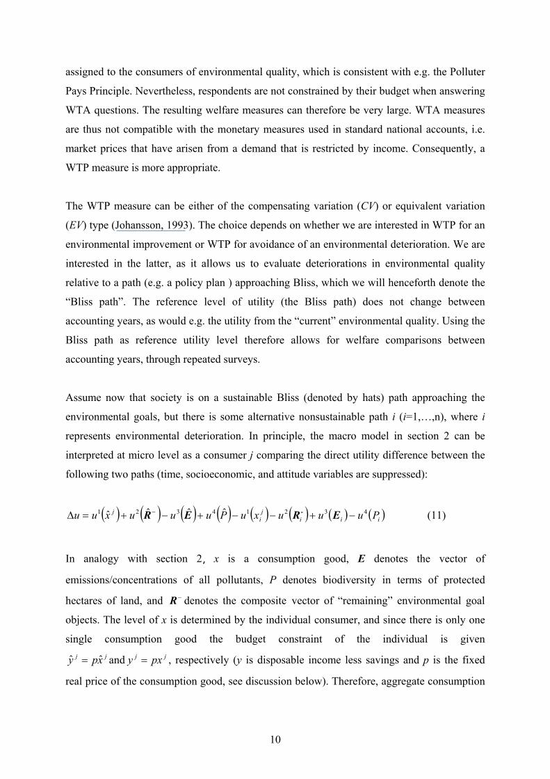
interpreted at micro level as a consumer j comparing the direct utility difference between the

following two paths (time, socioeconomic, and attitude variables are suppressed):

( ) ( ) ( ) ( ) ( ) ( ) ( ) ( )iiij

ij PuuuxuPuuuxuu 43214321 ˆˆˆˆ −+−−+−+=∆ − ERER - (11)

In analogy with section 2, x is a consumption good, E denotes the vector of

emissions/concentrations of all pollutants, P denotes biodiversity in terms of protected

hectares of land, and −R denotes the composite vector of “remaining” environmental goal objects. The level of x is determined by the individual consumer, and since there is only one

single consumption good the budget constraint of the individual is given jj xpy ˆˆ = and jj pxy = , respectively (y is disposable income less savings and p is the fixed

real price of the consumption good, see discussion below). Therefore, aggregate consumption

11

expenditure, or consumption, in the economy is ∑∑ ∀∀==

jj

jj yxpC ˆˆˆ and

∑∑ ∀∀==

jj

jj yxpC . For convenience, the superscript j is omitted in the following. By

assumption, the levels of E, P, and −R are the same for all individuals j.

Since direct utility is not observable, we need a monetary measure to evaluate the change in

utility. We have previously assumed that the subutility functions are homothetic. A commonly

used functional form satisfying these conditions is a linear utility function (Hanemann, 1984),

which is in correspondence with the linearization in equation (8):

iiii dPaxPdxau −+−−+−+=∆ −− cEbREcRb ˆˆˆˆ (12)

The parameters (or vectors of parameters) a b c and d represent the marginal utility of each of

the arguments in the utility function. The budget constraint of the consumer can be rewritten

as pyx = and

pyxˆˆ = , which allows us to express (12) in indirect utility terms, v:

iii dPpyaPd

pya −+−−+−+=∆ − cEbREcRb -ˆˆˆˆ

v (13)

The utility function is not directly observable, and we therefore use the EV measure to

evaluate this utility change. We want to measure the value to avoid environmental

deteriorations, relative to the Bliss path:

iii dPpyaPd

pEVya +−+=+−+

− −

∧

cEbREcRb -ˆˆˆ (14)

Rearranging, we can solve for∧

EV to avoid deviations from the Bliss path and obtain:

( ) ( ) ( )a

PPpda

pa

-pEV iii −+

−−=

∧ ˆˆˆ EEcRRb --

(15)

12

On the individual consumer level, equation (14) corresponds to equation (9). By assumption,

we have initially endowed the consumer with the Bliss path level of environmental and

natural resources. Therefore, the adjustments in NDP indicated by equation (9) should be

measured in terms of deviations from the Bliss levels of E, P, and −R , as indicated by

equation (15) . The components apd

ap

ap ,, cb essentially convey the result by Mäler (1974),

that the marginal willingness to pay (MWTP) for an environmental good can be expressed in

terms of the price of any private good and the marginal utilities of that good and the

environmental good. Exemplifying with biodiversity we have (Freeman, 1993):

∂∂∂

∂−=

xu

Pu

pMWTPP (16)

This corresponds to apd , since d is the marginal utility of biodiversity and a is the marginal

utility of the private composite good. The price p is in the context of satellite accounts fixed,

and determined by the price vector used in the national accounts during the year. Therefore,

we can use, e.g., the consumer price index to compare WTP estimates obtained during

different accounting years. If during each successive year t the economy is moving towards

Bliss according to some policy plan, the estimate given by (16) each year can be interpreted as

a Lindahl price for the public good in question (Varian, 1992). Equation (16) can also be

viewed as an inverse demand curve based on Roy’s identity (Kolstad and Braden, 1992). In

the current setting, equation (16) is a Hicksian (compensated) demand concept, because

income is adjusted to keep utility constant across the changes in P (Varian, 1992). Moreover,

the marginal utility of income is a/p (cf. equation (13)) across all changes. MWTP is a

counterpart to the market prices used in standard national accounts. It corresponds to what is

sometimes referred to as a “virtual price” for the public good (Carson, Flores and Hanemann,

1998). In this light, we see that (15) essentially gives the expenditure on environmental goods

as a function of virtual prices and quantity change. As is clear from equation (14), the price of

the composite private good only determines the expenditure on environmental goods.

Accordingly, the additive utility function allows for a two stage budgeting process, given by

equations (14) and (15). In the first stage (14), the consumer determines his/her EV WTP to

avoid a deviation from the policy plan (Bliss path) approaching Bliss, i.e. “achievement of the

13

national environmental goals”. This would give a total environmental “budget” each year that

could be compared between accounting years, irrespective of whether specific environmental

goods (or goals) are included or deleted from the valuation task in the future. In the second

stage (15), the consumer allocates budget shares to each of the specific environmental

problems. These budget shares are then determined by the respective parts in the sum (15).

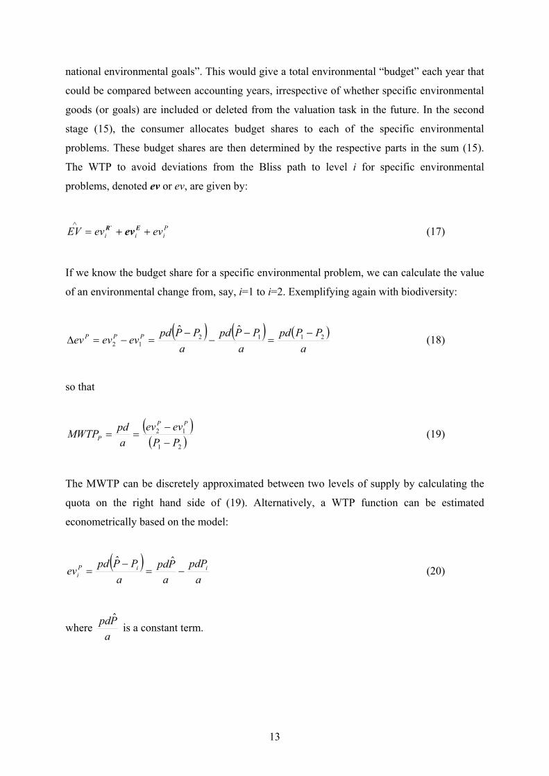
The WTP to avoid deviations from the Bliss path to level i for specific environmental

problems, denoted ev or ev, are given by:

Piii evevEV ++=

∧ER ev

-

(17)

If we know the budget share for a specific environmental problem, we can calculate the value

of an environmental change from, say, i=1 to i=2. Exemplifying again with biodiversity:

( ) ( ) ( )a

PPpda

PPpda

PPpdevevev PPP 211212

ˆˆ −=

−−

−=−=∆ (18)

so that

( )( )21

12

PPevev

apdMWTP

PP

P −−

== (19)

The MWTP can be discretely approximated between two levels of supply by calculating the

quota on the right hand side of (19). Alternatively, a WTP function can be estimated

econometrically based on the model:

( )a

pdPa

Ppda

PPpdev iiP

i −=−

=ˆˆ

(20)

where a

Ppd ˆ is a constant term.

14

Summing ( )( )21

12,or,,,,PPevev

apdevevEV

PPPiii −

−∧ER ev

-

across all individuals we obtain the

aggregate WTP or MWTP estimates for a representative consumer (assuming a utilitarian

welfare function; Johansson, 1993).

The correctness of the Hicksian demand concept outlined above hinges on prices and income

remaining unaffected throughout the changes, and that the environmental objects are of a pure

public good nature. If not, the effect of environmental changes on the utility of the household

is also dependent on the effect of changes in prices and income. For environmental satellite

accounting purposes, this contingent scenario is realistic. In this setting, respondents are

assumed to reveal their ex post annual WTP to have obtained the environmental change in

question during the year, conditional on the prices and incomes (and taxes) that were

prevailing during that year. This is due to environmental accounts being satellites to standard

national accounts, which employ prevailing market prices and income. Thus, any deviation

from standard national accounts with respect to prices and income would render the WTP

estimates incompatible with those accounts, and possibly also result in double-counting

errors. Hence, we can derive the marginal values of environmental goods at different levels of

provision for a specific accounting year. These values are the closest possible estimates

comparable to market pricesii.

Indeed, Backlund (2000) shows that a static MWTP measure of the type suggested here is

useful for constructing a welfare indicator, especially when environmental quality is linear

with respect to the stock of environmental “bads”. The necessary information is how a

consumer values a marginal reduction of environmental “bads” at time t. The static

approximation is then revised repeatedly as new MWTP information becomes available.

Backlund (2000) also shows that the MWTP measure should be revised more frequently if

environmental quality is nonlinear with respect to the stock of environmental “bads”.

4. Methodological Aspects on an Empirical Application

Next, the problem is what environmental goods should be included empirically and how they

should be handled in the survey framework. The answer to this question is far from

straightforward. For instance, in Sweden 15 very broadly defined national environmental

goals have been stipulated.iii These goals should be reached by the year 2020

(Naturvårdsverket, 2000). Within these goals, at least 60 environmental public good

15

“dimensions” can be identified. Valuing all these dimensions would be an enormous task.

Some authors argue that one should not even try to value a large number of environmental

goods in the same survey instrument, since the description of each good will by necessity

become too brief for respondents to properly understand (Carson and Mitchell, 1995).

Therefore, some sort of aggregation is necessary in order to reach a “manageable” number of

environmental goods.

4.1. Valuation objects

In selection of environmental goods to be valued we have used the SEEA criteria as our

guideline. To start from the relevance of the results for decision making, a list of

environmental issues targeted in the 15 national goals can be cut down considerably by the

limitation of availability of the basic physical data. Our focus will evidently be on those

phenomena that can be measured in physical terms (such as pollutants and emissions in

tons/micrograms per year). Therefore, our proposal covers achievement of the environmental

goals in general, with special focus on:

- Climate change (emissions of CO2 in tons)

- Acidification (emissions of SO2 and NOx in tons)

- Urban air quality (average concentrations of NO2, soot, benzene, toluene and particles in

microgram/m3)

- Nutrification (emissions of N in tons)

- Biodiversity (hectares of protected forestland).

On behalf of the Swedish government, the Environmental Advisory Council has chosen these

five objects as green indicators for Sweden with respect to emission levels and the state of the

environment (Anon, 1999). These indicators ”…are intended to reflect major environmental

problems” and ”…are intended to provide decision-makers and the public with readily

comprehensible information.” (Skr, 1999, p. 8). Even though the number of our valuation

objects do not cover all possible relevant environmental issues in Sweden, we think that our

subsample is not only manageable but also comprehensive in coverage of phenomena and

values so that the CVM can be tested in an accounting context. In addition, the results for the

environmental issues covered should be appropriate in the sense that about 20 national

Swedish regulatory agencies and authorities have issued their first reports on how they intend

to achieve the 15 overarching environmental goals adopted. General policies and concrete

16

policy measures to meet the targets set up for environmental policy, including economic

instruments, are currently planned and discussed actively both nationally and internationally.

Thus, there is a policy relevant basis for formulation of CVM scenarios and WTP

measurement with respect to the Bliss path and alternative future paths for environmental

quality in Sweden. In the following we consider an empirical approach for measuring WTP

as described in the theoretical sections.

4.2. Survey context

Firstly, as our application involves national environmental goals for Sweden, we are

interested in a representative nationwide sample. This can be obtained through official

Swedish registers. In the following sections we describe the general layout of the survey

instrument, as it reflects our various considerations during the survey development process.

We are interested in estimating an “environmental budget” and marginal values for the five

environmental objects previously mentioned (cf. equation (15)). Focus groups and a test

survey revealed that a comprehensive survey including all five problems would be too

demanding for the respondent to answer. Therefore, the survey is divided into several

versions. Since we have five specific valuation objects, and three levels of change for each

environmental object, we propose fifteen survey versions in total. All versions contain a

question on WTP to achieve all 15 environmental goals. This is then interpreted as aggregate

WTP to avoid deteriorations from the Bliss path (i.e. ∧

EV ). Each version would then contain a

detailed description of one environmental problem (i.e. either of climate change, acidification,

urban air quality, nutrification, or biodiversity) at one level of change. The respondent would

be asked how much of his/her aggregate WTP for the environmental goals that should be

allocated to the specific change. Furthermore, there would be one “rating” version of the

survey, where the respondent is asked to allocate 100 “points” to all five problems depending

on their relative importance. In this version, no detailed information would be given about the

valuation objects, and no specific environmental changes are suggested. Consequently, the

“rating” version would measure WTP to avoid deviations from the Bliss path for all five

problems, evaluated simultaneously by the respondent.

Recalling that R is the universal set of all 15 environmental goal objects, we introduce the

subscript l for climate change (l=1), acidification (l=2), urban air quality (l=3), and

17

nutrification (l=4), respectively. For the three different levels of change relative to the Bliss

path (i=1, 2, 3), the following information would then be obtainable from the individual

respondent for the biodiversity survey version:

Pii evevEV P +=

∧ -R (21)

where PP~=-R , and { }PP ,-RR = .

For the climate change, acidification, urban air quality, and nutrification survey versions we

have:

ll Eii evevEV +=

−∧R (22)

where ll E~=-R , and { }ll E,-RR = .

Equation (21) or (22) then gives the aggregate WTP of the individual respondent for the Bliss

path (environmental budget), and WTP to avoid deterioration from Bliss to i for valuation

object iP or lE . All “other” valuation objects are included in −R , and WTP for them is

implicitly given by -P

iev R or -l

iev R . Using the approaches indicated by equation (19) or (20),

MWTP can be estimated for a specific valuation object, based on WTP information for all

three levels i.

Finally, for the rating version, the following information would be obtainable:

PevevEV P ++=−∧

ER evE, (23)

where { }PP ,, ERR -E,= .

i.e. WTP for the Bliss path (environmental budget), and budget shares for all valuation object

to avoid deterioration from Bliss. However, no MWTP estimates can be obtained from this

survey version.

18

Equations (21)-(23) allows estimation of the different parts of equations (15) and (17).

Furthermore, it gives an opportunity to test the effects on WTP from different framings of the

valuation package. The information for the valuation task in the survey would be based on

available Swedish policy information regarding the national environmental goals (SOU

2000:52), and thorough review by experts at e.g. the Swedish Environmental Protection

Agency and the Swedish University of Agricultural Sciences. The reference utility (Bliss)

level is set at a level above the environmental goals, meaning that it will not be reached in the

near future, ensuring the possibility of repeated surveys using the same reference level. The

lower levels would correspond to the national environmental goals, and two alternative levels.

Each scenario would be formulated as a ten-year project, as this is the current first planning

period for the national environmental goals in Sweden.

For the sake of completeness, we will briefly touch upon relevant extensions of the presented

research, related specifically to CVM.

4.3. Further issues in a CVM application

The standard guidelines for a CVM scenario are: theoretically accurate, policy relevant,

plausible, understandable and meaningful (Carson, 1992). One important aspect of a plausible

scenario involves the inherent hypothetical nature of CVM surveys, i.e. that respondents are

not faced with an actual monetary transaction when answering WTP questions. The debate

has revolved around the question whether estimates based on such stated (hypothetical)

choices correspond to actual choices (NOAA, 1993). In various empirical investigations,

some authors have found substantial differences between actual and hypothetical valuation

(e.g. Bishop and Heberlein, 1979; Bohm, 1994; Cummings, Harrison and Rutström, 1995;

Seip and Strand, 1992), while others have not (e.g. Carson et al., 1996; Smith and Mansfield,

1998). When detected, several arguments have been put forward to explain this seemingly

unexpected difference, e.g. strategic behaviour (Bohm, 1994) or uncertainty (Bishop,

Heberlein and Kealy, 1983). Moreover, the disparity between responses to hypothetical and

actual WTP questions has in some situations been found to be systematic and predictable

(Blackburn, Harrison and Rutström, 1994). iv

In our view, the solution to this problem lies in explicitly addressing issues such as question

format, preference uncertainty, existing behavioral models, and respondent experience, when

developing the survey instrument.

19

As pointed out in the introductory section, an important feature of the present CVM

application is that it would be repeatable over time. Depending on the nature of the

environmental goods to be valued, the relevant time interval between surveys may vary.

Whitehead and Hoban (1999) develop a conceptual economic model based on behavioural

intentions, explaining how WTP may be expected to vary over time in a reliable CVM survey

instrument. They model WTP as a function of i.) individually perceived environmental

quality, which in turn is a function of government policy towards the environment, attitudes

(being influenced by demographic variables and time), and objective (i.e. actual)

environmental quality, ii.) the utility level of the consumer, and iii.) time. If the underlying

factors affecting WTP have not undergone significant changes between two surveys, a reliable

CVM instrument should not exhibit significantly different WTP values between the two

measurements. The reverse holds if any of the factors affecting WTP have changed over time.

Obviously, it is then important to consider these factors, to establish whether the survey

instrument is temporally reliablev. Thus, the first full-scale survey can still only be regarded as

a pilot survey in a temporal context, since the temporal reliability of the survey instrument can

only be assessed after the lapse of one or a few years. After repeating the survey, revisions of

the survey instrument may prove necessary.

5. Conclusions

In this paper, we have developed a model for environmental accounting that can be applied in

contingent valuation in a policy relevant manner.

The theoretical framework for our environmentally partially adjusted NDP indicates that we

can interpret the measure derived as the sustainable future income that an economy can enjoy

along the optimal path. This result is shown without the restrictive assumption of a constant

discount rate. The key to this is that we adopt the Ramsey device of writing the objective

function, or the integrand, as the deviation from “Bliss”, or sustainability. For an empirical

analysis, sustainability is determined by national environmental goals.

It is shown that the CVM framework can be formulated as an equivalent variation WTP

measure to avoid deviations from Bliss. This “environmental budget” can then be subdivided

to different environmental objects, using a two-stage budgeting process. By obtaining

information regarding different levels of environmental change, marginal WTP may be

estimated. Such a “virtual price” could, in turn, be used for green accounting purposes.

20

The next step would then be an integration of the model presented here into a state-of the-art

CVM application. This would account for issues such as question format, preference

uncertainty, behavioral models, and respondent experience. Most importantly, it would

involve a temporally reliable survey instrument. Pilot work on such applications is currently

carried out by researchers at the National Institute of Economic Research and the Swedish

University of Agricultural Sciences.

The values derived through the suggested survey instrument are, as always, contingent on the

scenario. It should therefore always be borne in mind that the use of these data out of context

is ultimately an arbitrary procedure. In particular, we believe that the resulting CVM data

should be used to calculate a separate adjusted NDP measure, and not be mixed with e.g.

results derived by using other valuation methods. This is logical, as we apply CVM because

we question whether other techniques adequately reflect the full economic value of the

resources of interest.

21

Acknowledgements

The authors would like to thank Professor Richard T. Carson, University of California,

Professor Per-Olov Johansson, Stockholm School of Economics, Professor Bengt Kriström,

Swedish University of Agricultural Sciences, Professor John Loomis, Colorado State

University, for helpful advice and suggestions. Furthermore, Dr. Göran Ericsson, Swedish

University of Agricultural Sciences, Professor Tom Heberlein, University of Wisconsin-

Madison, Professor John Loomis (again), Dr. Juha Siikamäki, University of California at

Davis, Dr. Matthew A. Wilson, University of Maryland, Eija Pouta and Mika Rekola,

University of Helsinki, are gratefully acknowledged for providing us with various types of

survey instruments and constructive comments on a pilot questionnaire. Kristian Skånberg,

Professor Lars-Erik Öller, and Dr Göran Östblom, all at the National Institute of Economic

Research (NIER), Stockholm, are gratefully acknowledged for commenting our work and

various versions of the present manuscript. Valuable discussions regarding policy and

questionnaire development as well as logistics have been provided by Roger Knudsen

(NIER), Viveka Palm and Anders Wadeskog, Statistics Sweden, as well as by Maria

Ingelsson, Swedish Environmental Protection Agency. Carl-Elis Boström, Ulla Bertills,

Håkan Staaf, and André Zuber, Swedish Environmental Protection Agency, and Anders

Wilander, Swedish University of Agricultural Sciences, have provided expert information and

comments regarding the environmental goals in Sweden. Sven Hellroth, National Institute of

Economic Research, has been most helpful in providing us with necessary literature. The

authors are solely responsible for the contents of the paper, and the views expressed are the

authors’ alone.

22

Notes i However, without strong separability, environmental goods could be substitutes, complements or independent in valuation. For qualitative and empirical results regarding the substitution between environmental goods, see e.g. Hoehn and Loomis (1993); Carson, Flores and Hanemann (1998); Brown et al. (1995); Neill (1995). Based on these studies, some conclusions can be drawn regarding a type of scope effect that is referred to as the embedding effect by Kahneman and Knetsch (1992), i.e. that WTP for a good may vary considerably depending on whether the good is valued on its own or as a part of a package: - If all public goods in a package are context independent, the sum of ceteris paribus independent valuations of these goods should equal the sum of the valuations when all goods are valued sequentially in a package. - If all public goods are Hicksian substitutes, the sum of ceteris paribus independent valuations of these goods should exceed the sum of the valuations when all goods are valued sequentially in a package. - If there are only two public goods, both of which are Hicksian complements, the sum of ceteris paribus independent valuations of these goods should fall short of the sum of the valuations of these two goods when they are valued sequentially in a package. - If there are more than two public goods, all of which are Hicksian complements, the sum of ceteris paribus independent valuations of these goods could exceed or fall short of the sum of the valuations when all goods are valued sequentially in a package. This underscores the importance not only of finding a policy relevant valuation package, but also of identifying the policy relevant valuation sequence.

ii However, for different accounting years, income changes (in terms of changes in lump-sum income, profit changes, and tax changes) should be added to the WTP measure to obtain social profitability (Johansson, 1993). iii Sweden's 15 environmental goals are: clean air, high quality groundwater, sustainable lakes and watercourses, flourishing wetlands, a balanced marine environment and sustainable coastal areas and archipelagos, no eutrophication, natural acidification only, sustainable forests, a varied agricultural landscape, a magnificent mountain environment, a good urban environment, a non-toxic environment, a safe radiation environment, a protective ozone layer, and limited influence on climate change. iv It should be noted that this difference is by no means restricted to WTP questions. O’Conor, Johanesson and Johansson (1999) observe a corresponding pattern, when asking respondents to perform the comparatively simple task of estimating how many kilometers they expect to travel by car during the next 12-month period. Green et al. (1998) arrive at similar results when asking respondents to estimate the height of the tallest redwood in California and the monthly gasoline consumption by an average US car owner. v Several CVM studies have shown temporal reliability of WTP estimates over time periods ranging from two weeks to five years, e.g., Carson et al., 1997; Berrens et al., 2000; Hasund, 1996; Stevens, More and Glass, 1994; Reiling et al. 1990. In contrast, Whitehead and Hoban (1999) make a comparison when there is time for significant change in factors affecting demand. Between 1990 and 1995, the attitudes toward the environment and governmental policy had become less favourable in the surveyed population and WTP estimates also decreased.

23

References Anon. 1999. Gröna nyckeltal – följ den ekologiska omställningen. Brochure from Miljövårdsberedningen.

Stockholm: Miljödepartementet.

Aronsson, T. and Löfgren, K.-G. 1999. Pollution tax design and `green' national accounting, European

Economic Review 43: 1457-1474.

Asheim, G.B. 1997. Adjusting green NNP to measure sustainability, Scandinavian Journal of Economics 99:

355-370.

Backlund, K. 2000. Welfare measurement, externalities and pigouvian taxation in dynamic economies. Umeå

University, Umeå economic studies 527. Umeå.

Berrens, R.P., Bohara, A.K., Silva, C.L., Brookshire, D. and McKee, M. 2000. Contingent values for New

Mexico instream flows: With tests of scope, group-size reminder and temporal reliability. Journal of

Environmental Management 58, 73-90.

Bishop, R.C. and Heberlein, T.A. 1979. Measuring values of extra-market goods: Are indirect measures biased?

American Journal of Agricultural Economics 61(5), 926-930.

Bishop, R.C., Heberlein, T.A. and Kealy, M.J. 1983. Contingent valuation of environmental assets: Comparisons

with a simulated market. Natural Resources Journal 23(3), 619-633.

Bjornstad, D.J. and Kahn, J.R. 1996. The contingent valuation of environmental resources: Methodological

issues and research needs. Cheltenham: Edward Elgar.

Blackburn, M, Harrison, G.W. and Rutström, E.E. 1994. Statistical bias functions and informative hypothetical

surveys. American Journal of Agricultural Economics 76, 1084-1088.

Boadway, R.W. and Bruce, N. 1993. Welfare Economics. Oxford: Blackwell.

Bohm,P. 1994. CVM spells responses to hypothetical questions. Natural resources journal 34, 37-49.

Brown, T.C., Barro, S.C., Manfredo, M.J., and Peterson, G.L. 1995. Does better information about the good

avoid the embedding effect? Journal of Environmental Management 44, 1-10.

Carson, R.T. 1992. Constructed markets. In Measuring the demand for environmental quality (eds. Braden, J.B.

and Kolstad, C.D.), 121-162. Amsterdam:North-Holland.

Carson, R.T. 2000. Contingent valuation: A user’s guide. Environmental Science and Technology 34, 1413-

1418.

Carson, R., Flores, N.E., and Hanemann, W.M. 1997. Sequencing and valuing public goods. University of

Boulder at Colorado, Department of Economics, Discussion Papers in Economics 97-21. Boulder.

Carson, R., Flores, N.E., and Hanemann, W.M. 1998. Sequencing and valuing public goods. Journal of

Environmental Economics and Management 36, 314-323.

Carson, R., Flores, N.E., Martin, K.M. and Wright, J.L. 1996. Contingent valuation and revealed preference

methodologies: Comparing the estimates for quasi-public goods. Land Economics 72(1), 80-99.

Carson, R.T., Hanemann, W.M., Kopp, R.J., Krosnick, J.A., Mitchell, R.C., Presser, S., Ruud, P.A. and Smith,

V.K. 1997. Temporal reliability of estimates from contingent valuation. Land Economics 73, 151-163.

Carson, R.T., and Mitchell, R.C. 1995. Sequencing and nesting in contingent valuation surveys. Journal of

Environmental Economics and Management 28, 155-173.

24

Cummings, R.G., Harrison, G.W. and Rutström, E.E. 1995. Homegrown values and hypothetical surveys: Is the

dichotomous choice approach incentive-compatible? The American Economic Review 85(1), 260-266.

Dasgupta, P., Kriström, B. and Mäler, K.-G. 1994. Current Issues in National Accounting, Working paper 107,

Department of Forest Economics, Swedish University of Agricultural Sciences.

Freeman, A.M. 1993. The Measurement of Environmental and Resource Values. Washington D.C.: Resources

for the Future.

Green, D., Jacowitz, K.E., Kahneman, D. and McFadden, D. 1998. Referendum contingent valuation, anchoring,

and willingness to pay for public goods. Resource and Energy Economics 20, 85-116.

Hanemann, W.M. 1984. Welfare evaluations in contingent valuation experiments with discrete responses.

American Journal of Agricultural Economics 66, 332-341.

Hartwick, J.M. 1990. Natural Resources, National Accounting and Economic Depreciation, Journal of Public

Economics 43:291-304.

Hasund, K.P. 1996. Time consistency of contingent value estimates. Draft manuscript, Department of

Economics, Swedish University of Agricultural Sciences.

Hoehn, J.P. 1991. Valuing the multidimensional impacts of environmental policy: Theory and methods.

American Journal of Agricultural Economics 73(2), 289-299.

Hoehn, J.P. and Loomis, J.B. 1993. Substitution effects in the valuation of multiple environmental programs.

Journal of Environmental Economics and Management 25, 56-75.

Johansson, P-O. 1993. Cost-benefit analysis of environmental change. Cambridge: Cambridge University Press.

Kahneman, D. and Knetsch, J.L. 1992. Valuing public goods: The purchase of moral satisfaction. Journal of

Environmental Economics and Management 22, 57-70.

Kolstad, C.D. and Braden, J.B. 1992. Environmental demand theory. In Measuring the demand for

environmental quality (eds. Braden, J.B. and Kolstad, C.D.), 17-39. Amsterdam:North-Holland.

Mitchell, R.C. and Carson, R.T. 1989. Using surveys to value public goods: The contingent valuation method.

Washington D.C.: Resources for the Future.

Mäler, K-G. 1974. Environmental economics: A theoretical inquiry. Baltimore: the Johns Hopkins University

Press for Resources for the Future.

Mäler, K.G. 1991. National Accounts and Environmental Resources, Environmental and Resource Economics 1:

1-15.

Naturvårdsverket. 2000. De Facto: Miljömålen – vår generations ansvar. Stockholm: Naturvårdsverket.

Neill, H.R. 1995. The context for substitutes in CVM studies: Some empirical observations. Journal of

Environmental Economics and Management 29, 393-397.

NOAA. 1993. Report of the NOAA Panel on contingent valuation. Federal Register 58 (10), 4601-14.

O’Conor, R.M., Johanesson, M. and Johansson, P-O. 1999. Stated preferences, real behaviour and anchoring:

Some empirical evidence. Environmental and Resource Economics 13, 235-248.

Ramsey, F. 1928. A Mathematical Theory of Saving, Economic Journal, 543-559.

Reiling, S.D., Boyle, K.J., Phillips, M.L. and Anderson, M.W. 1990. Temporal reliability of contingent values.

Land Economics 66(2), 129-134.

25

SEEA 2003. In press. Integrated Environmental and Economic Accounts. United Nations, European

Commission, International Monetary Fund, Organisation for Economic Co-operation and Development and

World Bank. New York: United Nations.

Seip, K. and Strand, J. 1992. Willingness to pay for environmental goods in Norway: A contingent valuation

study with real payment. Environmental and Resource Economics 2, 91-106.

Skr. 1999. Sustainable Sweden – A progress report on measures promoting ecologically sustainable

development. Regeringskansliet, Regeringens Skrivelser 1999/2000:13.

Smith, V.K. and Mansfield, C. 1998. Buying time: Real and hypothetical offers. Journal of Environmental

Economics and Management 36, 209-224.

SNA. 1993. System of National Accounts 1993. Commission of the European Communities, IMF, OECD, UN,

and The World Bank.

Solow, R.M. 1986. On the Intergenerational Allocation of Natural Resources, Scandinavian Journal of

Economics 88:141-149.

SOU 2000:52. 2000. Framtidens Miljö – Allas vårt ansvar! Slutbetänkande från Miljömålskommitén.

Stockholm: Fritzes.

Stevens, T.H., More, T.A. and Glass, R.J. 1994. Interpretation and temporal stability of CV bids for wildlife

existence: A panel study. Land Economics 70(3), 355-363.

Varian, H.R. 1992. Microeconomic analysis, Third edition. New York: Norton.

Weitzman, M.L. 1976. On the Welfare Significance of National Product in a Dynamic Economy, Quarterly

Journal of Economics 90: 156-162.

Whitehead, J.C., Haab, T.C. and Huang, J.-C. 1998. Part-whole bias in contingent valuation: Will scope effects

be detected with inexpensive survey methods? Southern Economic Journal 65(1), 160-168.

Whitehead, J.C. and Hoban, T.J. 1999. Testing for temporal reliability in contingent valuation with time for

changes in factors affecting demand. Land Economics 75(3), 453-465.

26

Titles in the Working Paper Series No Author Title Year

1 Warne, Anders and Anders Vredin

Current Account and Business Cycles: Stylized Facts for Sweden

1989

2 Östblom, Göran Change in Technical Structure of the Swedish Economy

1989

3 Söderling, Paul Mamtax. A Dynamic CGE Model for Tax Reform Simulations

1989

4 Kanis, Alfred and Aleksander Markowski

The Supply Side of the Econometric Model of the NIER

1990

5 Berg, Lennart The Financial Sector in the SNEPQ Model 1991

6 Ågren, Anders and Bo Jonsson

Consumer Attitudes, Buying Intentions and Consumption Expenditures. An Analysis of the Swedish Household Survey Data

1991

7 Berg, Lennart and Reinhold Bergström

A Quarterly Consumption Function for Sweden 1979-1989

1991

8 Öller, Lars-Erik Good Business Cycle Forecasts- A Must for Stabilization Policies

1992

9 Jonsson, Bo and Anders Ågren

Forecasting Car Expenditures Using Household Survey Data

1992

10 Löfgren, Karl -Gustaf, Bo Ranneby and Sara Sjöstedt

Forecasting the Business Cycle Not Using Minimum Autocorrelation Factors

1992

11 Gerlach, Stefan Current Quarter Forecasts of Swedish GNP Using Monthly Variables

1992

12 Bergström, Reinhold The Relationship Between Manufacturing Production and Different Business Survey Series in Sweden

1992

13 Edlund, Per-Olov and Sune Karlsson

Forecasting the Swedish Unemployment Rate: VAR vs. Transfer Function Modelling

1992

14 Rahiala, Markku and Timo Teräsvirta

Business Survey Data in Forecasting the Output of Swedish and Finnish Metal and Engineering Industries: A Kalman Filter Approach

1992

15 Christofferson, Anders, Roland Roberts and Ulla Eriksson

The Relationship Between Manufacturing and Various BTS Series in Sweden Illuminated by Frequency and Complex Demodulate Methods

1992

16 Jonsson, Bo Sample Based Proportions as Values on an Independent Variable in a Regression Model

1992

17 Öller, Lars-Erik Eliciting Turning Point Warnings from Business Surveys

1992

18 Forster, Margaret M Volatility, Trading Mechanisms and International Cross-Listing

1992

19 Jonsson, Bo Prediction with a Linear Regression Model and Errors in a Regressor

1992

20 Gorton, Gary and Richard Rosen

Corporate Control, Portfolio Choice, and the Decline of Banking

1993

21 Gustafsson, Claes-Håkan and Åke Holmén

The Index of Industrial Production – A Formal Description of the Process Behind it

1993

22 Karlsson, Tohmas A General Equilibrium Analysis of the Swedish Tax Reforms 1989-1991

1993

23 Jonsson, Bo Forecasting Car Expenditures Using Household Survey Data- A Comparison of Different Predictors

1993

27

24 Gennotte, Gerard and Hayne Leland

Low Margins, Derivative Securitites and Volatility 1993

25 Boot, Arnoud W.A. and Stuart I. Greenbaum

Discretion in the Regulation of U.S. Banking 1993

26 Spiegel, Matthew and Deane J. Seppi

Does Round-the-Clock Trading Result in Pareto Improvements?

1993

27 Seppi, Deane J. How Important are Block Trades in the Price Discovery Process?

1993

28 Glosten, Lawrence R. Equilibrium in an Electronic Open Limit Order Book 1993

29 Boot, Arnoud W.A., Stuart I Greenbaum and Anjan V. Thakor

Reputation and Discretion in Financial Contracting 1993

30a Bergström, Reinhold The Full Tricotomous Scale Compared with Net Balances in Qualitative Business Survey Data – Experiences from the Swedish Business Tendency Surveys

1993

30b Bergström, Reinhold Quantitative Production Series Compared with Qualiative Business Survey Series for Five Sectors of the Swedish Manufacturing Industry

1993

31 Lin, Chien-Fu Jeff and Timo Teräsvirta

Testing the Constancy of Regression Parameters Against Continous Change

1993

32 Markowski, Aleksander and Parameswar Nandakumar

A Long-Run Equilibrium Model for Sweden. The Theory Behind the Long-Run Solution to the Econometric Model KOSMOS

1993

33 Markowski, Aleksander and Tony Persson

Capital Rental Co st and the Adjustment for the Effects of the Investment Fund System in the Econometric Model Kosmos

1993

34 Kanis, Alfred and Bharat Barot

On Determinants of Private Consumption in Sweden 1993

35 Kääntä, Pekka and Christer Tallbom

Using Business Survey Data for Forecasting Swedish Quantitative Business Cycle Varable. A Kalman Filter Approach

1993

36 Ohlsson, Henry and Anders Vredin

Political Cycles and Cyclical Policies. A New Test Approach Using Fiscal Forecasts

1993

37 Markowski, Aleksander and Lars Ernsäter

The Supply Side in the Econometric Model KOSMOS 1994

38 Gustafsson, Claes-Håkan

On the Consistency of Data on Production, Deliveries, and Inventories in the Swedish Manufacturing Industry

1994

39 Rahiala, Markku and Tapani Kovalainen

Modelling Wages Subject to Both Contracted Increments and Drift by Means of a Simultaneous-Equations Model with Non-Standard Error Structure

1994

40 Öller, Lars-Erik and Christer Tallbom

Hybrid Indicators for the Swedish Economy Based on Noisy Statistical Data and the Business Tendency Survey

1994

41 Östblom, Göran A Converging Triangularization Algorithm and the Intertemporal Similarity of Production Structures

1994

42a Markowski, Aleksander Labour Supply, Hours Worked and Unemployment in the Econometric Model KOSMOS

1994

42b Markowski, Aleksander Wage Rate Determination in the Econometric Model KOSMOS

1994

43 Ahlroth, Sofia, Anders Björklund and Anders Forslund

The Output of the Swedish Education Sector 1994

44a Markowski, Aleksander Private Consumption Expendi ture in the Econometric Model KOSMOS

1994

28

44b Markowski, Aleksander The Input-Output Core: Determination of Inventory Investment and Other Business Output in the Econometric Model KOSMOS

1994

45 Bergström, Reinhold The Accuracy of the Swedish National Budget Forecasts 1955-92

1995

46 Sjöö, Boo Dynamic Adjustment and Long-Run Economic Stability

1995

47a Markowski, Aleksander Determination of the Effective Exchange Rate in the Econometric Model KOSMOS

1995

47b Markowski, Aleksander Interest Rate Determination in the Econometric Model KOSMOS

1995

48 Barot, Bharat Estimating the Effects of Wealth, Interest Rates and Unemployment on Private Consumption in Sweden

1995

49 Lundvik, Petter Generational Accounting in a Small Open Economy 1996

50 Eriksson, Kimmo, Johan Karlander and Lars-Erik Öller

Hierarchical Assignments: Stability and Fairness 1996

51 Url, Thomas Internationalists, Regionalists, or Eurocentrists 1996

52 Ruist, Erik Temporal Aggregation of an Econometric Equation 1996

53 Markowski, Aleksander The Financial Block in the Econometric Model KOSMOS

1996

54 Östblom, Göran Emissions to the Air and the Allocation of GDP: Medium Term Projections for Sweden. In Conflict with the Goals of SO2, SO2 and NOX Emissions for Year 2000

1996

55 Koskinen, Lasse, Aleksander Markowski, Parameswar Nandakumar and Lars-Erik Öller

Three Seminar Papers on Output Gap 1997

56 Oke, Timothy and Lars-Erik Öller

Testing for Short Memory in a VARMA Process 1997

57 Johansson, Anders and Karl -Markus Modén

Investment Plan Revisions and Share Price Volatility 1997

58 Lyhagen, Johan The Effect of Precautionary Saving on Consumption in Sweden

1998

59 Koskinen, Lasse and Lars-Erik Öller

A Hidden Markov Model as a Dynamic Bayesian Classifier, with an Application to Forecasting Business-Cycle Turning Points

1998

60 Kragh, Börje and Aleksander Markowski

Kofi – a Macromodel of the Swedish Financial Markets

1998

61 Gajda, Jan B. and Aleksander Markowski

Model Evaluation Using Stochastic Simulations: The Case of the Econometric Model KOSMOS

1998

62 Johansson, Kerstin Exports in the Econometric Model KOSMOS 1998

63 Johansson, Kerstin Permanent Shocks and Spillovers: A Sectoral Approach Using a Structural VAR

1998

64 Öller, Lars-Erik and Bharat Barot

Comparing the Accuracy of European GDP Forecasts

1999

65 Huhtala , Anni and Eva Samakovlis

Does International Harmonization of Environmental Policy Instruments Make Economic Sense? The Case of Paper Recycling in Europe

1999

66 Nilsson, Charlotte A Unilateral Versus a Multilateral Carbon Dioxide Tax - A Numerical Analysis With The European Model GEM-E3

1999

29

67 Braconier, Henrik and Steinar Holden

The Public Budget Balance – Fiscal Indicators and Cyclical Sensitivity in the Nordic Countries

1999

68 Nilsson, Kristian Alternative Measures of the Swedish Real Exchange Rate

1999

69 Östblom, Göran An Environmental Medium Term Economic Model – EMEC

1999

70 Johnsson, Helena and Peter Kaplan

An Econometric Study of Private Consumption Expenditure in Sweden

1999

71 Arai, Mahmood and Fredrik Heyman

Permanent and Temporary Labour: Job and Worker Flows in Sweden 1989-1998

2000

72 Öller, Lars-Erik and Bharat Barot

The Accuracy of European Growth and Inflation Forecasts

2000

73 Ahlroth, Sofia Correcting Net Domestic Product for Sulphur Dioxi de and Nitrogen Oxide Emissions: Implementation of a Theoretical Model in Practice

2000

74 Andersson, Michael K. And Mikael P. Gredenhoff

Improving Fractional Integration Tests with Bootstrap Distribution

2000

75 Nilsson, Charlotte and Anni Huhtala

Is CO2 Trading Always Beneficial? A CGE-Model Analysis on Secondary Environmental Benefits

2000

76 Skånberg, Kristian Constructing a Partially Environmentally Adjusted Net Domestic Product for Sweden 1993 and 1997

2001

77 Huhtala, Anni, Annie Toppinen and Mattias Boman,

An Environmental Accountant's Dilemma: Are Stumpage Prices Reliable Indicators of Resource Scarcity?

2001

78 Nilsson, Kristian Do Fundamentals Explain the Behavior of the Real Effective Exchange Rate?

2002

79 Bharat, Barot Growth and Business Cycles for the Swedish Economy

2002

80 Bharat, Barot House Prices and Housing Investment in Sweden and the United Kingdom. Econometric Analysis for the Period 1970-1998

2002

81 Hjelm, Göran Simultaneous Determination of NAIRU, Output Gaps and Structural Budget Balances: Swedish Evidence

2003

82 Huhtala, Anni and Eva Samalkovis

Green Accounting, Air Pollution and Health 2003

83 Lindström, Tomas The Role of High-Tech Capital Formation for Swedish Productivity Growth

2003

84 Hansson, Jesper, Per Jansson and Mårten Löf

Business survey data: do they help in forecasting the macro economy?

2003

85 Boman, Mattias, Anni Huhtala, Charlotte Nilsson, Sofia Ahlroth, Göran Bostedt, Leif Mattson and Peichen Gong

Applying the Contingent Valuation Method in Resource Accounting: A Bold Proposal