Sl No. Category of Creditor Amount Contingent Claims Amount of ...

Environmental and Resource Economics 20: 173–195, 2001.© 2001 Kluwer Academic Publishers. Printed in the Netherlands.
173
Addressing Negative Willingness to Pay inDichotomous Choice Contingent ValuationA Monte Carlo Simulation
ALOK K. BOHARA1, JOE KERKVLIET2 and ROBERT P. BERRENS1
1Department of Economics, University of New Mexico; 2Department of Economics, Oregon StateUniversity, Ballard Extension Hall, Room 303, Corvallis, Oregon, 97331, USA
Accepted 9 January 2001
Abstract. This paper has four purposes. First, we outline the controversy surrounding the issueof negative willingness to pay (WTP) in contingent valuation (CV) studies. Second, we use MonteCarlo simulation to examine the performance of alternative distributional assumptions in estimatingWTP in the presence of varying proportions of the population holding negative WTP values. Wefocus on dichotomous choice CV (DC-CV), where negative WTP values may be especially difficultto detect. Third, we extend the simulation to investigate the performance of the mixture models thathave recently been proposed for handling/identifying non-positive WTP values. Fourth, we extendthe simulation to investigate the performance of the nonparametric lower bound Turnbull approach.Results indicate that the relative performance of the DC-CV modeling alternatives evaluated here,which assume positive WTP, varies across the simulation setting (e.g., proportion of negative WTP);but none can be said to reasonably “solve” the problem ex post. This underscores the importance ofex ante efforts to identify if negative WTP is likely to be prominent in a given valuation setting. Insuch cases, appropriately handling negative WTP must be addressed through ex ante survey designand modeling choices that allow negative WTP.
Key words: contingent valuation, Monte Carlo simulation, negative willingness to pay
JEL classification: Q26
1. Introduction
The main objective of contingent valuation (CV) is to accurately represent peoples’preferences regarding nonmarket, often environmental, goods. Issues surroundingthe provision of non-marketed goods are usually complex and often controversial.It is not surprising that peoples’ opinions are heterogeneous.
This paper is concerned with a fundamental type of heterogeneity. Do all peoplethink an increase in the nonmarket good will make them better off, or at least noworse off? Or, for a proposed environmental policy change, is there a segment ofthe population that views the change in a negative way? Specifically, if presentedwith a standard valuation question (e.g., Hicksian willingness to pay to acquire thechange) for a posited increase in a environmental services, will some individualshave negative willingness to pay (WTP) for the change?
174 ALOK K. BOHARA ET AL.
Negative WTP presents a vexing problem to CV practitioners. In many studiesit is unclear how the question of negative value is addressed. However, zeroand/or negative values have already figured prominently in several CV studies anddiscussions.1 Lockwood et al. (1994, 1996), Keith et al. (1996), and Berrens et al.(1998) address the measurement of negative WTP, by asking valuation questionsto directly elicit these values. Kristom (1997) and Werner (1999) present mixturemodels to distinguish those who value the good positively from those who areindifferent. The empirical importance of such methods remains an open issue.
Some researchers argue that individuals expressing a negative WTP aremistaken in their assessment; that is, negative WTP might be in the data, but is dueto misperception of the good or context (Loomis and Ekstrand 1998). Sometimes,the assessed negative values are eliminated along with other “protest” responses(Jakobsson and Dragun 1996), or the estimated empirical distributions are trun-cated at zero when estimating mean or median WTP (Haab and McConnell 1998).More strongly, others implicitly deny the existence of negative WTP by advocat-ing the use of functional forms (e.g. Weibull, log-normal, log-logistic) that forcestrictly positive WTP estimates (Duffield and Patterson 1991; Carson et al. 1992,1998; Haab and McConnell 1997; Ekstrand and Loomis 1998). In contrast, manystudies estimate WTP using functional forms allowing positive, negative, or zeroWTP. An open questions is the gains or losses that arise from these contrastingdistributional assumptions.
This paper has four purposes. First, we outline the controversy surroundingnegative WTP in CV. Second, we use Monte Carlo simulation to examine theperformance of three distributional assumptions in estimating WTP in the pres-ence of varying proportions of the population holding negative WTP values. Thethree distributions are the normal, the log-normal, and the Weibull. The latter twodistributions are widely used in CV, but impose strictly positive WTP. We focus ondichotomous choice CV (DC-CV), the predominant elicitation format for valuationquestions and a format where negative WTP values may be especially difficultto detect. Third, we extend the simulation to investigate the performance of themixture models that have recently been proposed for handling/identifying non-positive WTP values. Fourth, for comparison purposes, we extend the simulationto investigate the performance of a nonparametric lower bound estimator, knownas the Turnbull approach, which imposes positive WTP.
2. Background
2.1. CONSIDERING NEGATIVE VALUES
CV is typically concerned with some proposed policy to implement a change fromq0 to q1, say, in a vector of environmental services, q, where q = {q1, q2, . . ., qn}.Suppose the change is posited in some fashion, either by the analyst or sponsoringagency, to be an improvement, q1 > q0. The issue is how people actually value theproposed change.

A MONTE CARLO SIMULATION 175
In addition to assuming rationality, well-behaved utility functions, etc., the CVresearcher typically initiates the valuation project with one of three maintainedhypotheses (Hanemann and Kanninen 1999). Two diametric hypotheses are:1) all individuals prefer q1 to q0;2) some individuals prefer q1 to q0, others are indifferent between q1 and q0, while
still others prefer q0 to q1.An intermediate maintained hypothesis is3) some individuals prefer q1 to q0, while others are indifferent between q1 and
q0.The bases for choosing one of these hypotheses will be a combination of theoret-ical guidance, extant empirical evidence, practical aspects of research design, andeconometric considerations.
2.2. THEORY
Regarding theory, Hanemann and Kanninen (1999) observe, “Economic theory perse cannot prescribe whether people like, dislike or are indifferent to the change inq.” More informally, Kristrom (1997, p. 1015) observes:
Many projects generate both winners and losers, including those generatingenvironmental benefits. Indeed, it is difficult to think of a project that does nothave a negative impact, however slight, on someone.
Conversely, Haab and McConnell (1997, 1998) contend that for most problemsaddressed by CV the notion of allowing negative WTP is “simply wrong”; thepublic good can typically be ignored if it does not provide utility. These contrastingviews seem to hinge on Haab and McConnell’s implied conception of freelydisposable public goods. If the goods in question are freely disposable, thentheir increased provision can “simply be ignored.” Lacking free disposablilty,some people may object to the project even if it were free. Some proportion ofthe population may suffer utility losses if the policy to move from q0 to q1 isimplemented.
Free disposability will not hold for those who have strong preferences regardingthe implementation of certain types of public policies. For example, in theirvaluation of a policy to restrict mining in favor of more intensive wildernessmanagement in the Kakadu region of the Northern Territory of Australia, Cameronand Quiggin (1994, p. 224) report
The issue in question was politically contentious and a large proportion of therespondents had strongly held views on the subject. Supporters of mining wereunlikely to state any positive willingness to pay (and might well have indicatednegative willingness to pay if asked.) The modal explanation among subjectswho answered “no” was a statement of the form ‘Support mining/good for thecountry.’

176 ALOK K. BOHARA ET AL.
Analogous views are likely to be held by some proportion of the population formany highly controversial environmental policies. Examples from the US Westwhere issues of negative WTP have been previously raised include: regional actionsto protect anadromous salmon stocks (Mathews and Johnson 1999), policies toreintroduce the wolf (Duffield 1993; Chadwick 1998; Wilson 1999), and policiesto reduce timber harvests to improve habitat for the endangered spotted owl (Castleand Berrens 1993).
The assumption of free disposability may be especially unrealistic when contro-versial environmental policies are multidimensional in nature. First, negative WTPcan arise in theory if the change from q0 to q1 involves reductions in other non-marketed goods. For example, management practices that favor wild stocks orendangered species, may reduce recreational fishing or hunting opportunities forother hatchery-reared stocks or game species (Hoobyar 1999). Further, there mightbe lost passive use values for changes in social fabric, disruption of communitiesand traditional ways and lifestyles, and thus associated negative WTP for theproposed change.2
Such “cultural values” are seldom targeted in CV, but this does not obviatetheir importance (Berrens et al. 1998). For example, Lockwood, et al. (1994, 1996)study the conflict between traditional cattle-raising lifestyles and environmentalrestoration in Australia promoted by grazing restrictions. They state (1996, p. 361):
The nonmarket benefits of continued grazing . . . [might be]: nonuse valueof heritage (the knowledge that grazing continues in the traditional mannerproviding a link with history); use value (benefits derived from using thearea while knowing that cattle are still grazed, or from seeing cattle, whichmay include visual appeal of cattle); indirect use value (value derived fromreading about, seeing pictures in books or on television, or hearing aboutcattle grazing). While this value framework has not previously been applied toheritage values in Australia, there seems no reason to suppose that such valuesdo not exist.
Finally, a further source of non-disposability, within the broadly defined policyproposal, is that some individuals may simply object to the method of payment(e.g. increased taxes), or the level of government involved (e.g., perceived loss ofstates rights or local control due to federal endangered species actions in the USfederal system) (Wilson 1999). These characteristics of a policy are unlikely to beregarded as “freely disposable” by some segment of the population.
2.3. EMPIRICAL EVIDENCE
In selecting one of the three maintained hypotheses, researches may also be guidedby previous empirical work. Here the evidence is not favorable to hypotheses (2)and (3), nor does it appear sensitive to the type of good in any obvious fashion.Some examples illustrate.

A MONTE CARLO SIMULATION 177
For environmental goods, Cameron and Quiggin (1994, 1998) find between33–37 percent respondents have negative WTP for increased emphasis on wilder-ness management. Lockwood, et. al (1996) report a mean negative WTP, sincevalues for continued grazing (and its deleterious effect on the environment) weregreater than those for the competing value of preserving the environment. Inanother Australian study of endangered species in Victoria, Australia, Jakobssonand Dragun (1996) find negative WTP estimates for about 20 percent of theirsample before “protest bids” are removed. In a split-sample test of scope effectsfor instream flow purchases to protect native fish in the Southwestern US, Berrenset al. (1996) estimate 29 and 15 percent of respondents have negative WTP for thesmaller and larger number of species protected, respectively. Ekstrand and Loomis(1998) and Loomis and Ekstrand (1998) restrict mean WTP to be positive forthreatened and endangered species protection, but find negative median WTP withsome model specifications and response treatments. In the two of four models esti-mated that do not impose positive WTP, Haab and McConnell (1997) find negativemean WTP for additional municipal taxes for beach cleanup.
For non-environmental goods, Berrens et al. (1997) estimate that a substan-tial proportion of students have a negative WTP for increased support of campuscultural centers. Donaldson, et al. (1996) specifically ask respondents whether theyvalue a reduced risk of food poisoning via irradiation, or whether they would bewilling to pay to avoid irradiated poultry. They find 15 percent of respondentshave a negative WTP for irradiation; that is they would pay to avoid it. When heestimates a linear logit model, Kristom (1997) finds a zero median and a negativemean WTP for a change in the fairways of Finnish ferries. Kristrom also estimatesthat 18 percent of respondents had negative WTP for a program to reduce traffic atStockholm’s Bromma airport.
2.4. PRACTICAL ASPECTS OF RESEARCH DESIGN
Careful research design and application potentially provide two ways to avoidor palliate problems with negative WTP. First, the argument is that it is alwayspossible to design the contingent scenario and proposed policy change so thatnegative aspects are completely eliminated. In other words, it is always possibleto design a good for valuation that is freely disposable for all the population. Thecounter arguments are several: a) This appears to be a strong judgement call on thepart of the researcher. How can the analyst ever be certain that she has eliminatedall of the negative, non-disposable aspects of the good, or the multidimensionalpolicy, being valued? b) In many instances the analyst is required to evaluate aspecific policy proposal and there is little latitude for trimming or isolating. c)Changing a policy proposal to eliminate all objections in a particular dimensionmay only lead to other objections on some other dimension (especially when thegood is multi-dimensional). d) Finally, the elimination of all negative aspects islikely to strain the plausibility of the valuation scenario. For example, one could

178 ALOK K. BOHARA ET AL.
attempt to value an environmental policy and state that it would not affect socialfabric, disrupt communities, or reduce other recreational opportunities. But, thisscenario is not likely to be taken seriously by respondents.
A second possible method of avoiding problems with negative WTP is tomodify CV methods. Haab and McConnell (1997) suggest qualitative researchprior to the final survey to establish cases where individuals have legitimatenegative values. Kristrom (1997) and Hanemann and Kanninen (1999) recommendscreening questions used prior to the valuation question. Once sub-samples aredifferentiated by positive and negative preferences (and possibly indifference), avariety of formal modeling approaches can be applied.
The recognition of legitimate negative WTP is a step in this direction, butremains uncommon and not well-investigated. In addition, these approaches giverise to four other issues: a) What proportion of the population with negative orzero WTP does it take to spoil standard modeling approaches and analyses? In thesimulation below, we present some evidence on this question. b) Such techniquesadd another layer of complexity and expense to CV research. c) Ex ante researchand screening questions to identify negative WTP will be subject to the same kindsof difficulties (e.g. framing and scope) as standard CV. d) Whether these methodsare worthwhile or necessary will depend, in part, on the ability of simple modelsbased on hypothesis (1) to accurately capture WTP. In the simulation below, wepresent some evidence on this issue.
2.5. ECONOMETRIC CONSIDERATIONS
A possible justification for employing hypotheses (2) or (3) is that, if negative WTPcould be ruled out a priori, a researcher can improve statistical efficiency by makingrestrictive but plausible distributional assumptions. However, such assumptionsmay come at a potentially high price. Most importantly, the imposition of positiveWTP may entail specification errors and ensuing biases. Also, a common approachfor imposing hypothesis (2) is to assume Weibull, log-normal or logistic distri-butions. Since these distributions have thick right-hand-side tails, their use yieldslarge variances and tend to inflate estimates of mean WTP (Haab and McConnell1997, 1998). In addition, forcing positive WTP in a probit model may create hetero-skedasticity problems, resulting in biased estimates of the WTP function (Greene1997, p. 888).
Imposing hypothesis (3) by means of a mixture model is less restrictive.However, this requires estimating one additional parameter and the performanceof this model has not been well investigated. In the simulation exercise below,we investigate the extent to which bias and efficiency are affected by imposinghypothesis (1). We also provide evidence on the conditions under which a mixturemodel is able to reliably and efficiently estimate WTP. For comparison, we alsoinvestigate the performance of the nonparametric lower bound Turnbull approach.
A MONTE CARLO SIMULATION 179
3. Monte Carlo Simulations
3.1. GENERATING TRUE WILLINGNESS TO PAY
We take as our fundamental starting point that some proportion of respondents,holding negative values for the proposed policy change, exists in the underlyingdistribution of WTP. The general data generating process (DGP) for our MonteCarlo simulation follows Elnagheeb and Jordan (1995). First, we begin by creatinga “true” willingness to pay, WTPi, i = 1, . . ., n, where n is the number of surveyrespondents, as:
WTPi = 30.0 − 5.0X1i + 0.01X2i + σεi .
This is the DGP. The X1i variable, generated uniformly over the range −5 to 5,represents an individual’s attitude towards the proposed policy change, coded suchthat those with a higher value have a more negative perception of the change, and alower WTP. Household income is represented by X2i, which is generated uniformlyover the range 10 to 80 (thousand of dollars), with an assumed positive impact onWTP. The DGP creates true WTP values that are normally distributed, with somefraction of the population having negative values.
The proportion of the negative values in the WTP series is dictated by the valuechosen for σ by using the formula: σ = −WTP/�−1(p), where the numerator is themean of the deterministic part of the WTP series, the denominator is the inverse ofthe normal distribution function, and p is the percentage of WTP values desired.To simulate the effect of different proportions of the population holding negativeWTP values, we choose three different values for p (0.05, 0.15, and 0.30) obtainingapproximately 0.02, 0.14 and 0.30 of negative WTP, respectively.
The issue of the appropriate bid structure in DC-CV has been much discussed,but no consensus has been reached. While it remains an important practical choiceby the analyst, it is not our primary focus. We follow Boyle et al. (1986) and use avector of 10 payment amounts (or “bids”), which is consistent with the suggestionof Alberini (1995). In the spirit of pretesting, 50 true WTP values are randomlysampled. We draw five uniform random numbers on the interval (0,1): p1, p2, p3,p4, p5. The quantiles corresponding to p1, p2, p3, p4, p5, (1 − p1), (1 − p2), (1 −p3), (1 − p4), (1 − p5) are calculated from the empirical distribution.
Next, we match individual WTPi’s to a particular randomly drawn bid to createa binary response variable Wi, where Wi = 1 represents a Yes response if WTP ≥bid, and Wi = 0 is a No response if WTP < bid. Each individual WTP is assignedequal probability of being matched with any bid. We do this by selecting WTP1
and randomly match it to a bid, then take WTP2 and randomly match it to a bid,and so on. Each WTPi is matched to one and only one bid.
Following the same general scheme, we simulate 500 draws for three differentsample sizes, 250, 500, and 1000. To simulate the effect of the three maintainedhypotheses of Section II, we employ various distributional assumptions whenestimating WTP. For hypothesis (1) we use the normal distribution, or linear probit.

180 ALOK K. BOHARA ET AL.
For hypothesis (2) we use both the log-normal and Weibull distributions, whichallow only allow positive WTP estimates. For hypothesis (3), we also use twomixture models (Hanemann and Kanninen 1999) using the log-normal and theWeibull distributions. We repeat all these for three different proportions of negativevalues, where approximately 2, 14 and 30 percent are obtained by the simulationapproach.
Once the WTP values are generated, the root mean squared error (RMSE) iscalculated as
√�(SWTPi − TWTP)2/n, where SWTP is the simulated series and
TWTP is the true WTP. The bias is calculated as the difference between the meanof the SWTP series and TWTP.
3.2. ESTIMATION
Using the (assumed) known values for the vector of explanatory variables Xi andthe values for Wi, i = 1, . . ., n, resulting from the matching of bids with WTPi, wedirectly estimate WTP functions following the approach of Cameron and James(1987). Dropping the subscripts, the response probability is:
Pr(yes) = Pr(W = 1) = 1 − Ge[X, A;β, κ] (1)
where X is the vector of explanatory variables (X1 and X2), κ is the shape parameter(−1/σ ), β is a vector of coefficients to be estimated, A is the bid ($), and Ge[·]is the distribution function. We use three different distributional assumptions fore. For example, if e follows an extreme value distribution, then the cumulativedensity function Ge[·] will be a Weibull. The other distributional assumptions arelog-normal and normal. The DGP is always normal though.
We also adopt a mixture distribution approach as advocated by Hanemann andKanninen (1999) and employed by Kristom (1997) and Werner (1999). We intro-duce an additional parameter γ to allow a spike at zero. We define a variable, Z,such that Z = 1 indicates a respondent who will never say Yes to any paymentamount (i.e. is either opposed or indifferent to the proposed policy change) andhas zero probability of changing her response if presented with a lower bid. IfZ = 0 the respondent says No to the bid, but is not inherently opposed or indif-ferent to the change and has a positive probability of changing her response(e.g., for a lower payment amount). Assume that the probabilities of being instates Z = 1 and Z = 0 are γ and (1 − γ ), respectively. The likelihood for theith individual is defined as the sum of the states multiplied by their associatedprobabilities:
Li = [Li|Z=0] ∗ (1 − γ ) + [Li |Z=1] ∗ γ (2)
Of those who say No to a payment, given that they are indifferent, the likelihoodof observing a no is 1, [Li|Z=1] = 1. Hence, the probability of saying No is:γ + (1 − γ )·Pr{No}. Of those who say Yes, given that they are indifferent, the
A MONTE CARLO SIMULATION 181
likelihood of observing a Yes is 0, Li|Z=1 = 0. The probability of saying Yes thenreduces to: (1 − γ )·Pr{Yes}. The total likelihood function is:
L = �W=1[(1 − γ ) ∗ (1 − Ge[X, A;β, κ])]�W=0[γ + (1 − γ )
+Ge[X, A;β, κ]] (3)
In addition to the parametric approaches, we also generated simulation resultsusing a non-parametric, distribution-free lower-bound WTP estimator known as theTurnbull approach (Haab and McConnell 1997). The Turnbull approach is basedon the probability or frequency information for Yes responses in a DC format andassumes non-negative values. It provides a conservative lower bound estimate ofWTP because it assumes that the mass of the empirical distribution falling betweenany two payment amounts, A($), falls at the lowest value of the interval.3
4. Results
We now turn to assessing the performance of the three distributions in estimatingWTP when negative WTP values are held by various proportions of the population.First, we use standard methods of estimating WTP functions and then we use themixture model approach. In all cases, samples of three different sizes (n = 250, n= 500, and n = 1000) were drawn from a population wherein true WTP (TWTP)is distributed normally with mean $30.00 and standard deviation that varies withthe proportion of the population with negative WTP. For each sample, we employthree commonly used distributional assumptions to estimate TWTP: the normal,log-normal, and Weibull. For the normal distributional assumption, predictions ofnegative WTP can occur. For the log-normal and Weibull, only positive predictionsof WTP can occur, even though some fraction of the population holds negativevalues.
4.1. STANDARD ESTIMATION METHODS
Tables I–III present the results of the Monte Carlo simulations for the three,progressively larger population proportions with negative WTP. In Table I, theproportion of those holding negative WTP (about 2 percent) seems to be at aninnocuous level. In practice, such a low incidence of negative WTP is likely to beundetected or ignored by the analyst.
In Table II, a substantial portion of the population (about 14 percent) has anegative WTP. In field studies, it is unlikely that this level of negative WTP wouldbe ignored as a statistical accident. Still, we do not know the extent to which theresults from a misspecified model will be affected by the existence of this normallydistributed proportion of negative WTP.
In Table III, we increase the fraction of the population with negative WTPto a hefty 30 percent. At this level of negative WTP, the analyst might consider

182 ALOK K. BOHARA ET AL.
Table I. Simulation results (∼= 2% negative WTP).
Simulated WTP series (SWTP)
Distributions Mean Standard Bias Median RMSE 95% 90%
deviation CI CI
n = 250
(σ = 8.03, TWTP = 29.87, % negative values = 2.23)
Normal 29.94 1.02 0.07 29.90 1.02 28.14, 32.08 28.36, 31.66
Log-normal 29.05 1.43 −0.82 29.01 1.65 26.38, 31.79 26.84, 31.42
Weibull 28.75 1.22 −1.12 28.72 1.65 26.46, 31.16 26.87, 30.67
n = 500
(σ = 7.96, TWTP = 29.59, % negative values = 2.50)
Normal 29.59 0.75 0.0 29.63 0.74 28.06, 30.98 28.33, 30.79
Log-normal 26.27 0.94 −3.32 26.28 3.45 24.34, 28.13 24.68, 27.75
Weibull 26.85 4.84 −2.74 26.64 5.55 24.72, 28.42 25.00, 28.16
n = 1000
(σ = 7.97, TWTP = 29.63, % negative values = 2.40)
Normal 29.63 0.51 0.0 29.65 0.51 28.62, 30.60 28.78, 30.49
Log-normal 28.76 0.78 −0.87 28.71 1.17 27.38, 30.39 27.58, 30.05
Weibull 28.25 0.58 −1.38 28.24 1.49 27.08, 29.45 27.31, 29.20
Notes: Five hundred samples are drawn for each simulation. RMSE is calculated as√�(SWTPi − TWTP)2/n, where SWTP is the simulated series and TWTP is the true WTP.
Intercept and slope parameters are 30, −5, and 0.01. The 95% confidence intervals (CI), forexample, are 0.025 and 0.975 percentile values of the empirical distribution of the simulatedseries. The binary data are generated using the normal distribution. The bias is calculated asthe difference between the mean SWTP series and TWTP.
modifying data collection and interpretation and statistical procedures in order toaccount for negative WTP.
As seen in Table I, the assumption of a normal distribution leads to accurateestimates for all three sample sizes with 2 percent negative WTP in the DGP. Theestimates of central tendency (mean and median) of WTP are within a few penniesof the TWTP obtained in the sample. Both 90 and 95 percent confidence intervalscontain the TWTP. Although this positive performance is not affected by samplesize, the two measures of dispersion (standard deviation and RMSE) are reducedby half as sample size is increased from n = 250 to n = 1000.
For the log-normal and Weibull distributions, the results are less positive. Meanand median estimates are consistently less than TWTP and the precision of the esti-mates suffers in comparison to the use of the normal distribution. Both the standarddeviation estimates and the RMSE are larger for the log-normal and Weibulldistributions than for the normal. In about half the cases, the 90 and 95 percent

A MONTE CARLO SIMULATION 183
Table II. Simulation results (∼=14% negative WTP).
Simulated WTP (SWTP)
Distributions Mean Standard Bias Median RMSE 95% 90%
deviation CI CI
n = 250
(σ = 23.31, TWTP = 29.87, % negative values = 13.65)
Normal 29.94 2.31 −0.07 29.96 2.30 25.33, 34.31 26.31, 33.85
Log-normal 36.08 4.04 −6.21 35.58 7.40 30.30, 44.93 30.79, 42.51
Weibull 33.07 2.52 −3.20 32.93 4.08 28.96, 38.42 29.35, 37.15
n = 500
(σ = 23.09, TWTP = 29.59, % negative values = 13.75)
Normal 29.61 1.67 0.02 29.66 1.67 26.44, 32.71 26.83, 32.21
Log-normal 62.51 17.06 32.92 58.86 37.07 40.33, 111.0 43.04, 96.09
Weibull 33.28 3.17 3.69 33.07 4.86 28.49, 41.44 28.90, 39.52
n = 1000
(σ = 23.12, TWTP = 29.63, % negative values = 13.86)
Normal 29.65 1.05 0.02 29.69 1.05 27.43, 31.67 27.91, 31.33
Log-normal 36.85 2.24 7.22 36.50 7.56 33.21, 41.81 33.59, 40.77
Weibull 32.48 1.24 2.85 32.44 3.11 30.36, 35.06 30.71, 34.51
Notes: Five hundred samples are drawn for each simulation. RMSE is calculated as√�(SWTPi − TWTP)2/n, where SWTP is the simulated series and TWTP is the true WTP.
Intercept and slope parameters used are 30, −5, and 0.01. The 95% confidence intervals(CI), for example, are 0.025 and 0.975 percentile values of the empirical distribution of thesimulated series. The binary data are generated using the normal distribution. The bias iscalculated as the difference between the mean SWTP and TWTP.
confidence intervals do not contain the TWTP. It appears that the inappropriateimposition of skewness that follows from the use of the log-normal and Weibulldistributions results in a performance deterioration. The direction of this deteri-oration is surprising. The skewed distributions give underestimates of TWTP; theoutcome is most pronounced when n = 500. Still, the deterioration is not serious.For the n = 250 and n = 1000 cases, the TWTP is estimated fairly closely whenusing any of the distributions. It appears that when only a minuscule proportion ofthe population have preferences implying negative WTP, these three distributionalassumptions provide reasonable and practically useful estimates of TWTP centraltendency and dispersion.
Table II shows the results of increasing the proportion of negative WTP holdersto 14 percent in the DGP. Here the normal distribution again performs well. Theestimates of the mean and median using the normal distribution are very close to
184 ALOK K. BOHARA ET AL.
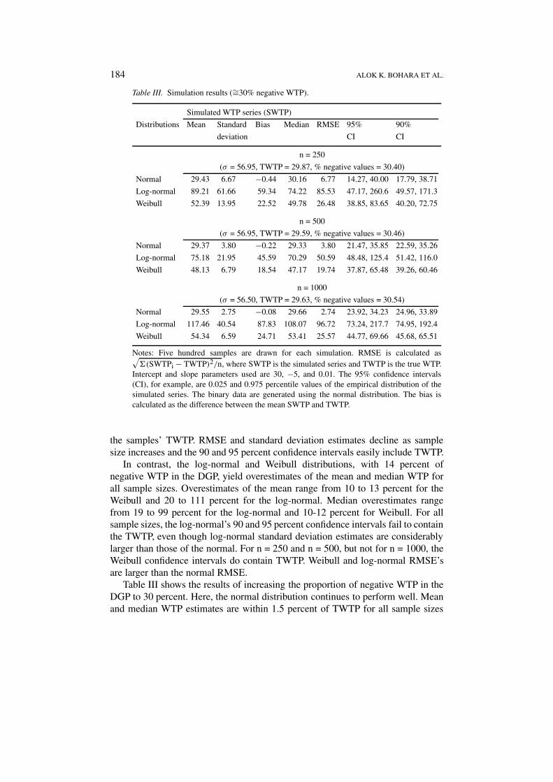
Table III. Simulation results (∼=30% negative WTP).
Simulated WTP series (SWTP)
Distributions Mean Standard Bias Median RMSE 95% 90%
deviation CI CI
n = 250
(σ = 56.95, TWTP = 29.87, % negative values = 30.40)
Normal 29.43 6.67 −0.44 30.16 6.77 14.27, 40.00 17.79, 38.71
Log-normal 89.21 61.66 59.34 74.22 85.53 47.17, 260.6 49.57, 171.3
Weibull 52.39 13.95 22.52 49.78 26.48 38.85, 83.65 40.20, 72.75
n = 500
(σ = 56.95, TWTP = 29.59, % negative values = 30.46)
Normal 29.37 3.80 −0.22 29.33 3.80 21.47, 35.85 22.59, 35.26
Log-normal 75.18 21.95 45.59 70.29 50.59 48.48, 125.4 51.42, 116.0
Weibull 48.13 6.79 18.54 47.17 19.74 37.87, 65.48 39.26, 60.46
n = 1000
(σ = 56.50, TWTP = 29.63, % negative values = 30.54)
Normal 29.55 2.75 −0.08 29.66 2.74 23.92, 34.23 24.96, 33.89
Log-normal 117.46 40.54 87.83 108.07 96.72 73.24, 217.7 74.95, 192.4
Weibull 54.34 6.59 24.71 53.41 25.57 44.77, 69.66 45.68, 65.51
Notes: Five hundred samples are drawn for each simulation. RMSE is calculated as√�(SWTPi − TWTP)2/n, where SWTP is the simulated series and TWTP is the true WTP.
Intercept and slope parameters used are 30, −5, and 0.01. The 95% confidence intervals(CI), for example, are 0.025 and 0.975 percentile values of the empirical distribution of thesimulated series. The binary data are generated using the normal distribution. The bias iscalculated as the difference between the mean SWTP and TWTP.
the samples’ TWTP. RMSE and standard deviation estimates decline as samplesize increases and the 90 and 95 percent confidence intervals easily include TWTP.
In contrast, the log-normal and Weibull distributions, with 14 percent ofnegative WTP in the DGP, yield overestimates of the mean and median WTP forall sample sizes. Overestimates of the mean range from 10 to 13 percent for theWeibull and 20 to 111 percent for the log-normal. Median overestimates rangefrom 19 to 99 percent for the log-normal and 10-12 percent for Weibull. For allsample sizes, the log-normal’s 90 and 95 percent confidence intervals fail to containthe TWTP, even though log-normal standard deviation estimates are considerablylarger than those of the normal. For n = 250 and n = 500, but not for n = 1000, theWeibull confidence intervals do contain TWTP. Weibull and log-normal RMSE’sare larger than the normal RMSE.
Table III shows the results of increasing the proportion of negative WTP in theDGP to 30 percent. Here, the normal distribution continues to perform well. Meanand median WTP estimates are within 1.5 percent of TWTP for all sample sizes
A MONTE CARLO SIMULATION 185
and the 90 and 95 percent confidence intervals contain TWTP. In contrast, usingof the positively skewed log-normal and Weibull distributions systematically leadsto substantive overestimates of WTP. Standard deviation estimates, while largerthan those from the normal distribution are insufficiently large to indicate the errorin these estimates. Neither the log-normal nor the Weibull confidence intervalscontain TWTP for any sample size.
The log-normal results mislead substantially more than the Weibull’s. The log-normal mean estimate is 154 percent over TWTP for n = 500 and 296 percent whenn = 1000. Weibull overestimates range from 62 percent (n = 500) to 83 percent(n = 1000). It is disturbing that the performance of these distributions does notimprove, and in some cases deteriorates, with sample size. Relative to the normal,log-normal RMSE is 12 times larger for n = 250 and 34 times larger for n = 1000.Weibull RMSE is 3 times larger for n = 250 and 8 times larger for n = 1000.
4.2. MIXTURE MODEL ESTIMATION
In this section, we follow the recommendation of Hanemann and Kanninen (1999),and the recent examples of Kristrom (1997) and Werner (1999), and estimate WTPusing a mixture distribution approach (see equation 3). Tables IV–VI report theresults for the three different percentages of negative WTP.
In the case of 2% with negative WTP in the DGP (Table IV) the performance ofthe two distributions hardly differs from the non-mixture model method (see TableI). Both distributions underestimate WTP and the underestimation is most seriouswhen n = 500. However, the underestimation is not large; ranging from 10 percent(n = 500) to less than 5 percent (n = 1000). Two differences that do emerge withthe mixture models concern the estimated value of γ and root mean squared error(RMSE). The estimated γ value indicates that a small percentage of the populationhas zero WTP values. In 5 of the six simulations, the estimated γ value under-estimates this proportion of the population. Compared to the standard estimationprocedure, the mixture models also lead to increases in root mean squared error(RMSE). In each case RMSE with the mixture model is at least twice that obtainedwith the standard model using the same distribution and substantially larger thanthe RMSE of the normal model.
Table V presents the mixture model results when 14 percent negative WTPvalues in the DGP. The Weibull and log-normal mixture models outperform thestandard model procedures for these distributions, but still fail to out-perform thenormal model. In comparison with the results of Table II, the mixture model resultsin Table V show that biases in both mean and median estimates are reduced; biasesrange from 2 to 23 percent. Both the mixture models’ 90 and 95 percent confidenceintervals contain TWTP for all sample sizes. Also, for both distributions, RMSEis reduced by the use of the mixture models. When the mixture log-normal modelis used, the estimated γ value closely matches the proportion of the populationwith non-positive WTP for all three sample sizes. In contrast, the Weibull mixture

186 ALOK K. BOHARA ET AL.
Table IV. Mixture models, simulation results (∼=2% negative WTP).
Simulated WTP series (SWTP)
Distributions Mean Standard Bias Median RMSE 95% 90%
deviation CI CI
n = 250
(σ = 8.03, TWTP = 29.87, % negative values = 2.23)
Log-normal 28.76 4.26 −1.11 28.65 4.40 26.35, 31.39 26.80, 30.82
(average γ̂ = 2.32)
Weibull 28.75 1.21 −1.12 28.74 2.70 26.55, 31.29 26.90, 30.66
(average γ̂ = 1.29)
n = 500
(σ = 7.96, TWTP = 29.59, % negative values = 2.50)
Log-normal 26.53 1.60 −3.06 26.58 11.95 24.41, 28.63 24.72, 28.41
(average γ̂ = 1.82)
Weibull 26.65 1.01 −2.94 26.64 9.66 24.68, 28.52 24.97, 28.22
(average γ̂ = 1.29)
n = 1000
(σ = 7.97, TWTP = 29.63, % negative values = 2.40)
Log-normal 28.21 0.56 −1.42 28.20 2.32 27.11, 29.37 27.32, 29.16
(average γ̂ = 1.80)
Weibull 28.42 1.09 −1.21 28.35 2.65 27.24, 29.58 27.45, 29.30
(average γ̂ = 1.47)
Notes: Five hundred samples are drawn for each simulation. RMSE is calculated as√�(SWTPi − TWTP)2/n, where SWTP is the simulated series and TWTP is the true WTP.
Intercept and slope parameters used are 30, −5, and 0.01. The 95% confidence intervals (CI),for example, are 0.025 and 0.975 percentile values of the empirical distribution of the simulatedseries. The binary data are generated using the normal distribution. The bias is calculated as thedifference between the mean SWTP and TWTP. Simulated WTP values are calculated as the meanof (1 − γ̂ )∗SWTP.
model provides a substantial underestimate of non-positive WTP for n = 250 and n= 1000.
Although log-normal and Weibull mixture models appear to be fairly accuratewhen a small fraction of the population has negative WTP, their performancebegins to deteriorate as the proportion increases to 30 percent in the DGP. Theresults in Table IV show that both mixture models consistently overestimate WTP.For the Weibull the overestimate of the mean ranges from 39 to 45 percent. Forthe log-normal, the overestimates range from 43 to 71 percent. This is an improve-ment over standard use of the log-normal and Weibull distributions, but the 90and 95 percent confidence intervals still fail to contain TWTP for any sample size.Compared to the performance of the normal distribution (Table III), the Weibull

A MONTE CARLO SIMULATION 187
Table V. Mixture models, simulation results (∼=14% negative WTP).
Simulated WTP series (SWTP)
Distributions Mean Standard Bias Median RMSE 95% 90%
deviation CI CI
n = 250
(σ = 23.31, TWTP = 29.87, % negative values = 13.65)
Log-normal 36.92 17.42 7.05 33.32 18.78 28.17, 74.24 28.76, 50.59
(average γ̂ = 13.62)
Weibull 32.51 2.62 2.64 32.30 3.72 28.36, 38.14 28.90, 36.73
(average γ̂ = 5.39)
n = 500
(σ = 23.09, TWTP = 29.59, % negative values = 13.75)
Log-normal 30.75 1.70 1.16 30.72 2.05 27.51, 34.15 28.04, 33.61
(average γ̂ = 13.70)
Weibull 30.14 4.92 0.55 30.26 4.95 26.96, 33.53 27.58, 32.81
(average γ̂ = 12.51)
n = 1000
(σ = 23.12, TWTP = 29.63, % negative values = 13.86)
Log-normal 32.19 1.95 2.56 31.82 3.22 29.46, 37.31 29.81, 35.79
(average γ̂ = 12.63)
Weibull 31.89 1.72 2.26 31.69 2.84 29.57, 34.61 29.85, 34.16
(average γ̂ = 5.43)
Notes: Five hundred samples are drawn for each simulation. RMSE is calculated as√�(SWTPi − TWTP)2/n, where SWTP is the simulated series and TWTP is the true WTP.
Intercept and slope parameters used are 30, −5, and 0.01. The 95% confidence intervals (CI),for example, are 0.025 and 0.975 percentile values of the empirical distribution of the simulatedseries. The binary data are generated using the normal distribution. The bias is calculated as thedifference between the mean SWTP and TWTP. Simulated WTP values are calculated as themean of (1 − γ̂ )∗SWTP.
and log-normal mixture models nearly always have higher standard deviations andRMSE.
On the positive side, the results indicate that mixture models are able to detectthe presence of a substantive proportion of those holding non-positive WTP. Eachestimate of γ in Table VI indicates that over 20 percent of the population does nothold positive WTP values.
4.3. TURNBULL APPROACH
For the Turnbull approach, a non-parametric lower bound WTP estimator, simula-tion results for the cases with approximately 2, 14 and 30 percent negative WTP

188 ALOK K. BOHARA ET AL.
Table VI. Mixture models, simulation results (∼=30% negative WTP).
Simulated WTP series (SWTP)
Distributions Mean Standard Bias Median RMSE 95% 90%
deviation CI CI
n = 250
(σ = 56.95, TWTP = 29.87, % negative values = 30.40)
Log-normal 51.01 54.12 21.14 43.19 58.05 34.39, 97.59 35.66, 67.41
(average γ̂ = 35.37)
Weibull 43.46 8.23 13.59 42.20 15.89 33.93, 59.96 35.17, 53.94
(average γ̂ = 27.34)
n = 500
(σ = 56.95, TWTP = 29.59, % negative values = 30.46)
Log-normal 47.63 12.80 18.04 44.25 22.11 35.16, 57.43 36.39, 54.26
(average γ̂ = 28.80)
Weibull 43.04 5.56 13.45 42.09 14.55 35.16, 57.43 36.39, 54.26
(average γ̂ = 21.89)
n = 1000
(σ = 56.50, TWTP = 29.63, % negative values = 30.54)
Log-normal 42.42 4.20 12.79 42.20 13.46 37.24, 49.10 37.82, 48.19
(average γ̂ = 34.67)
Weibull 41.11 2.52 11.48 40.78 11.75 36.65, 46.11 37.34, 45.08
(average γ̂ = 30.42)
Notes: Five hundred samples are drawn for each simulation. RMSE is calculated as√�(SWTPi − TWTP)2/n, where SWTP is the simulated series and TWTP is the true WTP.
Intercept and slope parameters used are 30, −5, and 0.01. The 95% confidence intervals (CI),for example, are 0.025 and 0.975 percentile values of the empirical distribution of the simulatedseries. The binary data are generated using the normal distribution. The bias is calculated as thedifference between the mean SWTP and TWTP. Simulated WTP values are calculated as the meanof (1 − γ̂ )∗SWTP.
in the DGP are provided in Tables VII, VIII and IX, respectively. The Turnbullapproach, which allows only positive WTP, never outperforms the normal model.
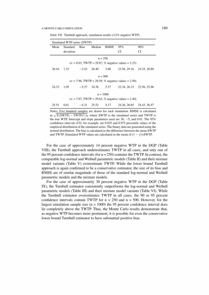
For the case where the proportion with negative WTP in the DGP is small(approximately 2 percent in Table VII), the Turnbull estimator performs similarlyto the log-normal and Weibull parametric models (Table I) and the mixture models(Table IV). Specifically, it underestimates TWTP and none of the 90 or 95 percentCI’s contain TWTP. The lower bound Turnabull approach is confirmed to be aconservative estimator; while its simulated estimates of mean WTP are in the rangeof $25, they are always slightly lower than the parametric alternatives and thushave the largest negative biases (varying from −3.43 to −5.27 across the differentsimulation sample sizes).
A MONTE CARLO SIMULATION 189
Table VII. Turnbull approach, simulation results (∼=2% negative WTP).
Simulated WTP series (SWTP)
Mean Standard Bias Median RMSE 95% 90%
deviation CI CI
n = 250
(σ = 8.03, TWTP = 29.87, % negative values = 2.23)
26.44 1.33 −3.43 26.40 3.68 23.94, 29.16 24.25, 28.80
n = 500
(σ = 7.96, TWTP = 29.59, % negative values = 2.50)
24.33 1.05 −5.27 24.38 5.37 22.34, 26.33 22.56, 25.96
n = 1000
(σ = 7.97, TWTP = 29.63, % negative values = 2.40)
25.51 0.61 −4.31 25.52 4.17 24.26, 26.65 24.43, 26.47
Notes: Five hundred samples are drawn for each simulation. RMSE is calculatedas
√�(SWTPi − TWTP)2/n, where SWTP is the simulated series and TWTP is
the true WTP. Intercept and slope parameters used are 30, −5, and 0.01. The 95%confidence intervals (CI), for example, are 0.025 and 0.975 percentile values of theempirical distribution of the simulated series. The binary data are generated using thenormal distribution. The bias is calculated as the difference between the mean SWTPand TWTP. Simulated WTP values are calculated as the mean of (1 − γ̂ )∗SWTP.
For the case of approximately 14 percent negative WTP in the DGP (TableVIII), the Turnbull approach underestimates TWTP in all cases, and only one ofthe 95 percent confidence intervals (for n = 250) contains the TWTP. In contrast, thecomparable log-normal and Weibull parametric models (Table II) and their mixturemodel variants (Table V) overestimate TWTP. While the lower bound Turnbullapproach is again confirmed to be a conservative estimator, the size of its bias andRMSE are of similar magnitude of those of the standard log-normal and Weibullparametric models and the mixture models.
For the case of approximately 30 percent negative WTP in the DGP (TableIX), the Turnbull estimator consistently outperforms the log-normal and Weibullparametric models (Table III) and their mixture model variants (Table VI). Whilethe Turnbull estimator overestimates TWTP in all cases, the 90 or 95 percentconfidence intervals contain TWTP for n = 250 and n = 500. However, for thelargest simulation sample size (n = 1000) the 95 percent confidence interval doeslie completely above the TWTP. Thus, the Monte Carlo results demonstrate that,as negative WTP becomes more prominent, it is possible for even the conservativelower bound Turnbull estimator to have substantial positive bias.
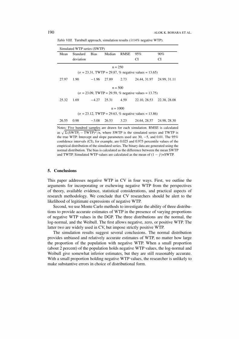
190 ALOK K. BOHARA ET AL.
Table VIII. Turnbull approach, simulation results (∼=14% negative WTP).
Simulated WTP series (SWTP)
Mean Standard Bias Median RMSE 95% 90%
deviation CI CI
n = 250
(σ = 23.31, TWTP = 29.87, % negative values = 13.65)
27.97 1.90 −1.96 27.89 2.73 24.44, 31.97 24.99, 31.11
n = 500
(σ = 23.09, TWTP = 29.59, % negative values = 13.75)
25.32 1.69 −4.27 25.31 4.59 22.10, 28.53 22.38, 28.08
n = 1000
(σ = 23.12, TWTP = 29.63, % negative values = 13.86)
26.55 0.98 −3.08 26.53 3.23 24.64, 28.57 24.98, 28.30
Notes: Five hundred samples are drawn for each simulation. RMSE is calculatedas
√�(SWTPi − TWTP)2/n, where SWTP is the simulated series and TWTP is
the true WTP. Intercept and slope parameters used are 30, −5, and 0.01. The 95%confidence intervals (CI), for example, are 0.025 and 0.975 percentile values of theempirical distribution of the simulated series. The binary data are generated using thenormal distribution. The bias is calculated as the difference between the mean SWTPand TWTP. Simulated WTP values are calculated as the mean of (1 − γ̂ )∗SWTP.
5. Conclusions
This paper addresses negative WTP in CV in four ways. First, we outline thearguments for incorporating or eschewing negative WTP from the perspectivesof theory, available evidence, statistical considerations, and practical aspects ofresearch methodology. We conclude that CV researchers should be alert to thelikelihood of legitimate expressions of negative WTP.
Second, we use Monte Carlo methods to investigate the ability of three distribu-tions to provide accurate estimates of WTP in the presence of varying proportionsof negative WTP values in the DGP. The three distributions are the normal, thelog-normal, and the Weibull. The first allows negative, zero, or positive WTP. Thelatter two are widely used in CV, but impose strictly positive WTP.
The simulation results suggest several conclusions. The normal distributionprovides unbiased and relatively accurate estimates of WTP, no matter how largethe proportion of the population with negative WTP. When a small proportion(about 2 percent) of the population holds negative WTP values, the log-normal andWeibull give somewhat inferior estimates, but they are still reasonably accurate.With a small proportion holding negative WTP values, the researcher is unlikely tomake substantive errors in choice of distributional form.

A MONTE CARLO SIMULATION 191
Table IX. Turnbull approach, simulation results (∼=30% negative WTP).
Simulated WTP series (SWTP)
Mean Standard Bias Median RMSE 95% 90%
deviation CI CI
n = 250
(σ = 56.95, TWTP = 29.87, % negative values = 30.40)
35.25 3.46 5.37 35.24 6.39 28.09, 41.91 29.58, 41.08
n = 500
(σ = 56.95, TWTP = 29.59, % negative values = 30.46)
30.88 2.89 1.29 30.85 3.16 25.72, 36.37 26.42, 35.81
n = 1000
(σ = 56.50, TWTP = 29.63, % negative values = 30.54)
33.12 1.84 3.50 33.21 3.95 29.75, 36.62 30.18, 36.24
Notes: Five hundred samples are drawn for each simulation. RMSE is calculatedas
√�(SWTPi − TWTP)2/n, where SWTP is the simulated series and TWTP is
the true WTP. Intercept and slope parameters used are 30, −5, and 0.01. The 95%confidence intervals (CI), for example, are 0.025 and 0.975 percentile values ofthe empirical distribution of the simulated series. The binary data are generatedusing the normal distribution. The bias is calculated as the difference between themean SWTP and TWTP. Simulated WTP values are calculated as the mean of(1 − γ̂ )∗SWTP.
As the proportion of the population with negative WTP increases to 14 percent,the Weibull, and especially log-normal, distributions give positively biased esti-mates of WTP, and appear to have no statistical advantage over the normal model.As the proportion of the population with negative WTP increases from 14 to 30percent, the use of the log-normal and Weibull become increasingly untenable.They both begin to grossly overestimate WTP. Also, the Weibull or log-normalmodels never out-perform the normal model.
Third, we extend the simulation to investigate the performance of mixturemodels that have recently been proposed for handling/identifying non-positiveWTP values. Using mixture models of the log-normal and Weibull distribu-tions leads to an improvement in the performance of these distributions. Mixturemodeling decreases bias and reduces errors compared to the standard models usingthese distributions. Although, mixture models fail to out-perform the standard useof the normal distribution, especially when 30 percent hold negative WTP values,they do provide fairly accurate estimates of the proportion of the population withnegative WTP.
Fourth, for comparison to the parametric approaches, we also use Monte Carlomethods to evaluate the performance of the nonparametric Turnbull approach for
192 ALOK K. BOHARA ET AL.
estimating WTP. The Turnbull approach never outperforms the normal model, andis confirmed to be a conservative estimator in many cases. In the case wherenegative WTP is negligible (approximately 2 percent) or relatively negligible(approximately 14 percent) the bias is negative and the Turnbull approach under-estimates WTP. In such cases, there is no evidence to prefer the Turnbull approachover the parametric models (or the mixture model versions) even when the distribu-tional assumption is known to be wrong (e.g., log-normal and Weibull). However,as the proportion of the population with negative WTP grows (to approximately30 percent) the results show that the Turnbull approach outperforms the parametricmodels (including the mixture model versions) where the distributional assumptionis known to be wrong (i.e., log-normal and Weibull).
In summary, as expected Monte Carlo results suggest that under a normal DGPthe normal distribution provides superior estimates of WTP for a wide range ofthe population holding negative values. If negative WTP is somehow known, apriori, to be incidental in the data, it can probably be ignored. The choice ofdistribution can be safely made on other grounds. Lacking a priori knowledge,mixture models can be used to help identify substantive negative WTP. But, ifnegative WTP is prominent in the data, using distributional assumptions that forcepositive WTP can lead to large overestimates and one should not be very confidentof the estimates obtained from mixture models. Further, in cases where negativeWTP is negligible, the conservative, nonparametric Turnbull estimator performsas expected and underestimates WTP. However, as negative WTP becomes moreprominent, the Turnbull approach may itself overestimate WTP.
In closing, if negative WTP is prominent in a given data set, none of the DC-CV modeling alternatives evaluated here that assume positive WTP will reasonably“solve” the problem ex post. In such cases, appropriately handling negative WTPmust be addressed through modeling choices that allow negative WTP. This conclu-sion also underlines the need for ex ante research design efforts to help researchersidentify whether negative WTP is prominent in a given valuation setting. If found,then the focus turns to modeling approaches that accomodate negative WTP. Suchapproaches remain relatively under-investigated, and there is room for considerableresearch effort. For example, as a final caveat, in our Monte Carlo simulationsthe DGP assumes that the negative component of the WTP values has the samedistribution as the positive component (e.g., normal). As noted by an anonymousreviewer, in reality this might not be the case. These two types of values for sameenvironmental policy may have very different statistical properties, and assumingotherwise may itself be the source of considerable error. We leave consideration ofsuch issues to future research.

A MONTE CARLO SIMULATION 193
Acknowledgements
We thank Charles Mason, Shawna Grosskopf, participants in the 1999 Universityof Oregon, Northwest Conference on Environmental and Resource Economics,and several anonymous reviewers for helpful comments. No lead authorship isassigned.
Notes
1. Examples in the context of discrete choice CV include: Bowker and Stoll 1988; Cameron andQuiggin 1994; Bateman et al. 1995; Berrens et al. 1997; Cameron and Englin 1997.
2. It is conceptually possible that individuals may have negative nonmarket values for the job lossesor displacement associated with a proposed environmental policy change (Rosenthal and Nelson1992; Hausman 1993, p. 388; Castle et al. 1994; Portney 1994, p. 13). But, as an anonymousreviewer notes, this is an especially problematic issue. From a general equilibrium perspective,apparent job losses may really be transfers to another region or sector of the economy. Valuingthese losses in a nonmarket context introduces serious potential for double counting if theyare elsewhere being evaluated in market context (e.g., employment and income impacts from aregional economic model). However, it is possible that individuals value the particular distribu-tion of jobs in a given sector and geographic location, and this is related to cultural heritage andlifestyle issues. Mathews and Johnson (1999) argue that the total level of employment may notbe the key issue; e.g., they attempt to measure passive use values for avoiding job displacementassociated with salmon preservation.
3. The expected Turnbull estimator is, E(WTP) =∑M+1
j=1 Aj−1pj with the variance defined as∑M+1
j=1 A2j−1(V(Gj + V(Gj−1)) -
∑Mj=1Aj Aj−1V(Gj ), where the Aj are the payment amounts
(j = 1, . . ., M), p = probability density function, g = cumulative distribution function. The
log-likelihood is LnL =∑M
j=1[Nj ln(∑j
i pi ) + (1 − Nj )ln(∑j
i pi )], where Nj = number ofrespondents saying no to Aj . For details see Haab and McConnell (1997).
References
Alberini, A. (1995), ‘Testing Willingness to Pay Models of Discrete Choice Contingent ValuationData’, Land Economics 71, 83–95.
Bateman, I., I. Langford, K.Turner, K. Willis and G. Garrod (1995), ‘Elicitation and TruncationEffects in Contingent Valuation Studies’, Ecological Economics 12, 93–106.
Berrens, R., A. Bohara and J. Kerkvliet (1997), ‘A Randomized Response Approach to DichotomousChoice Contingent Valuation’, American Journal of Agricultural Economics 79, 275–290.
Berrens, R., D. Brookshire, P. Ganderton and M. McKee (1998), ‘Exploring the Nonmarket SocialImpacts of Environmental Policy Change’, Resource and Energy Economics 19, 117–138.
Berrens, R., P. Ganderton and C. Silva (1996), ‘Valuing the Protection of Minimum Instream Flowsin New Mexico’, Journal of Agricultural and Resource Economics 21, 294–309.
Bowker, M. and J. Stoll (1988), ‘Use of Dichotomous Choice Nonmarket Methods to Value theWhooping Crane Resource’, American Journal of Agricultural Economics 70, 372–381.
Boyle, K., M. Welsh and R. Bishop (1986), ‘Validation of Empirical Measures of Welfare Change’,Land Economics 64, 94–98.
Cameron, T. and J. Englin (1997), ‘Respondent Experience and Contingent Valuation of Environ-mental Goods’, Journal of Environmental Economics and Management 33, 296–313.
Cameron, T. and M. James (1987), ‘Efficient Estimation Methods for Close-Ended ContingentValuation Surveys’, Review of Economics and Statistics 69, 269–276.

194 ALOK K. BOHARA ET AL.
Cameron, T. and J. Quiggin (1994), ‘Estimation Using Contingent Valuation Data from a “Dichoto-mous Choice with Follow-up” Questionnaire’, Journal of Environmental Economics andManagement 27, 218–234.
Cameron, T. and J. Quiggin (1998), ‘Estimation Using Contingent Valuation Data from “Dichoto-mous Choice with Follow-up” Questionnaire: Reply’, Journal of Environmental Economics andManagement 35, 195–199.
Carson, R. T., W. M. Hanemann, R. J. Kopp, S. Presser and P. Rund (1992), A Contingent ValuationStudy of Lost Passive Use Values Resulting from the Exxon Valdez Oil Spill. Anchorage, AK:Report for the Attorney General of the State of Alaska.
Carson, R. T., W. M. Hanemann, R. J. Kopp, J. A. Krosnick, R. C. Mitchell, S. Presser, P. A. Rund, V.K. Smith, M. Conaway and K. Martin (1998), ‘AReferendum Design and Contingent Valuation:The NOAA-Panel’s No-Vote Recommendation’, Review of Economics and Statistics 80, 335–338.
Castle, E. and R. Berrens (1993), ‘Economic Analysis, Endangered Species and the Safe MinimumStandard’, Northwest Environmental Journal 9, 108–130.
Castle, E., R. Berrens and R. Adams (1994), ‘Natural Resource Damage Assessment: Speculationsabout a Missing Perspective’, Land Economics 70, 378–385.
Chadwick, D. (1998), ‘The Return of the Grey Wolf’, National Geographic 193, 145–169.Donaldson, C., T. Mapp, M. Ryan and K. Curtin (1996), ‘Estimating the Economic Benefits of
Avoiding Food-Borne Risk: Is Willingness to Pay Feasible’, Epidemiology and Infection 116,285–294.
Duffield, J. (1993), An Economic Analysis of Wolf Recovery in Yellowstone Park: Visitor Attitudesand Values, Department of Economics. Missoula, MT: University of Montana.
Duffield, J. and D. Patterson (1991), ‘Inference and Optimal Design for a Welfare Measure inDichotomous Choice Contingent Valuation’, Land Economics 67, 225–239.
Ekstrand, E. and J. Loomis (1998), ‘Incorporating Respondent Uncertainty when Estimating Willing-ness to Pay for Protecting Critical Habitat for Threatened and Endangered Fish’, Water ResourcesResearch 34, 3149–3155.
Elnagheeb, A. and J. Jordan (1995), ‘Comparing Three Approaches that Generate Bids for the Refer-endum Contingent Valuation Method’, Journal of Environmental Economics and Management29, 92–104.
Greene, W. (1997), Econometric Analysis, 3rd edn. Upper Saddle River, NJ: Prentice Hall.Haab, T. and K. McConnell (1997), ‘Alternative Methods for Handling Negative Willingness to Pay
in Referendum Models’, Journal of Environmental Economics and Management 32, 251–270.Haab, T. and K. McConnell (1998), ‘Referendum Models and Economic Values: Theoretical,
Intuitive, and Practical Bounds on Willingness to Pay’, Land Economics 74, 216–229.Hanemann, W. H. and B. Kanninen (1999), ‘The Statistical Analysis of Discrete-Response CV Data’,
in I. Bateman and K. Willis, eds., Valuing Environmental Preferences: Theory and Practice ofthe Contingent Valuation Method in the US, EC and Developing Countries. Oxford, UK: OxfordUniversity Press.
Hausman, J., ed. (1993), Contingent Valuation: A Critical Assessment. New York: North Holland.Hoobyar, P. (1999). ‘Tensions Rise as Fishing Resumes for Coho off Oregon Coast’, Restoration.
Oregon Sea Grant Publication, Spring: 1–4. Corvallis, OR: Oregon State University.Jakobsson, K. and A. Dragun (1996), Contingent Valuation and Endangered Species. Cheltenham,
UK: Edward Elgar.Keith, J., C. Fawson and V. Johnson (1996), ‘Preservation or Use: A Contingent Valuation Study of
Wilderness Preservation in Utah’, Ecological Economics 18, 207–214.Kristrom, B. (1997), ‘Spike Models in Contingent Valuation’, American Journal of Agricultural
Economics 79, 1013–1023.Lockwood, M., J. Loomis and T. DeLacy. (1994), ‘The Relative Unimportance of Non-market
Willingness to Pay for Timber Harvesting’, Ecological Economics 9, 145–152.

A MONTE CARLO SIMULATION 195
Lockwood, M., P. Tracey and N. Klomp (1996), ‘Analyzing Conflict between Cultural Heritageand Nature Conservation in the Australian Alps: A CVM Approach’, Journal of EnvironmentalPlanning and Management 39, 357–370.
Loomis, J. and E. Ekstrand (1998), ‘Alternative Approaches for Incorporating Respondent Uncer-tainty when Estimating Willingness to Pay: The Case of the Mexican Spotted Owl’, EcologicalEconomics 27, 29–41.
Mathews, K. and F. R. Johnson (1999), ‘Damned if You Do and Damned if You Don’t: Nonuse StatedPreferences in Salmon Preservation Policy’, Technical Working Paper #T9903. North Carolina:Triangle Economic Research.
Portney, P. (1994), ‘The Contingent Valuation Debate: Why Economists Should Care’, Journal ofEconomics Perspectives 8, 3–17.
Rosenthal, D. and R. Nelson (1992), ‘Why Existence Values Should Not Be Used in Cost-BenefitAnalysis’, Journal of Policy Analysis and Management 11, 116–122.
Werner, M. (1999), ‘Allowing for Zeros in Dichotomous-Choice Contingent-Valuation Models’,Journal of Business and Economic Statistics 17, 479–486.
Wilson, P. (1999), ‘Wolves, Politics and the Nez Perce: Wolf Recovery in Central Idaho and the Roleof Native Tribes’, Natural Resources Journal 39, 543–564.

Copyright © 2022 FDOKUMEN