Spatiotemporal structures in the internally pumped optical parametric oscillator

Spatiotemporal structures in the internally pumped optical parametric oscillator

P. Lodahl,1 M. Bache,1,2 and M. Saffman3

1Optics and Fluid Dynamics Department, Riso” National Laboratory, Postbox 49, DK-4000 Roskilde, Denmark2Department of Mathematical Modelling, Technical University of Denmark, DK-2800 Lyngby, Denmark

3Department of Physics, University of Wisconsin, 1150 University Avenue, Madison, Wisconsin 53706�Received 31 August 2000; published 17 January 2001�

We analyze pattern formation in doubly resonant second-harmonic generation in the presence of a compet-ing parametric process, also named the internally pumped optical parametric oscillator. Different scenarios areestablished where either the up- or down-conversion processes dominate the spatiotemporal behavior. Thepossibility of obtaining exact solutions above threshold for the parametric oscillation process allows detailedanalytical investigations of the parametric instability, that are supplemented by numerical analysis. We identifysecondary instabilities that lead to formation of negative patterns and gray solitons. Estimates of the thresholdsfor pattern formation under experimentally relevant conditions are given.

DOI: 10.1103/PhysRevA.63.023815 PACS number�s�: 42.65.Sf, 42.65.Ky, 42.65.Tg

I. INTRODUCTION

Pattern formation in cavity enhanced � (2) nonlinear pro-cesses has been a flourishing research area recently. Patternsare formed due to transverse instabilities in the plane perpen-dicular to the propagation direction. Two fundamentally dif-ferent processes have been described that are the opticalparametric oscillator �OPO� �1–3� and second-harmonic gen-eration �SHG� �4–6�. The spontaneous formation of patternshas been attributed to an off-axis emission mechanism me-diated by the nonlinearity and diffraction when the intracav-ity fields are detuned slightly from cavity resonance. Thedetuning can either be introduced manually by scanning thecavity length or, in the case of SHG, occur as a nonlineareffect. The absence of nonlinear phase shifts in the OPOappears since patterns are generated directly at the paramet-ric oscillation threshold while an oscillation threshold doesnot exist in SHG. This is the major reason for the differencesbetween SHG and OPO.

Pattern formation under the combined processes of SHGwith competing nondegenerate parametric oscillations hasbeen treated recently both for singly resonant �7,8� and dou-bly resonant �9� SHG. This combined system, also named theinternally pumped optical parametric oscillator �IPOPO�,was shown to be of experimental relevance by Schiller et al.�10� in their work on efficient frequency doubling. Hence,the parametric fields can be generated in such a way that theyautomatically obey resonance conditions in the cavity, whichlowers the oscillation threshold. This additional decay pro-cess substantially alters the classical �11� as well as the quan-tum �12,13� behavior of SHG. The competing parametricprocess turns out to be of great relevance also for studies ofpattern formation in SHG.

Here we describe the formation of spatiotemporal struc-tures in doubly resonant SHG under the influence of thecompeting parametric process. The parametric process isfound to influence pattern formation in two fundamentallydifferent ways. For some parameters the instabilities seen ina pure SHG system, with the parametric process neglected,can exist, while completely different transverse structures areobserved in other regions. The SHG instabilities were previ-

ously studied by Etrich et al. �4� but the analysis presentedhere is generalized to include also the possibility of nonidealphase matching of the frequency conversion process in addi-tion to unequal propagation distances for the fundamentaland second harmonic. These extra degrees of freedom turnout to be usable tuning parameters in order to reach newparameter regions, especially for tuning the SHG instabilitieswith respect to the parametric threshold.

The instabilities due to the parametric process are studiedin detail in this paper. The simplicity of the parametric insta-bility allows derivation of exact solutions valid above theparametric threshold. Such exact solutions were previouslyfound in the externally pumped nondegenerate OPO byLonghi �3� and by Marte in the IPOPO without diffraction�11�. Depending on the sign of the fundamental detuning, theparametric fields are either emitted as homogeneous off-axisor on-axis waves in the cavity. None of these instabilitieslead to any spatially modulated intensity structure, but whilethe off-axis parametric solutions are proven to be linearlystable and hence quench pattern formation, the on-axis solu-tions can destabilize through a secondary instability. Thisinstability was previously found to lead to formation of com-plicated spatiotemporal structures, as, e.g., intensity spiralpatterns �14�. Here we will focus on other secondary insta-bilities of the IPOPO including a parametric bistability and aself-pulsing instability. They are found to lead to novel trans-verse structures such as honeycomb patterns and oscillatingdark solitons.

In addition to these studies of the rich pattern formationdynamics in the IPOPO, we also analyze a realistic experi-mental setup in order to address the question of the experi-mental realizability of the scheme. This is particularly rel-evant in light of the recent progress in the experimentalrealization of pattern formation in � (2) based resonators �15�.

II. BASIC MODEL

A. The configuration

Figure 1 shows the cavity configuration for doubly reso-nant SHG. The cavity consists of two independent arms forthe fundamental and the second-harmonic fields, respec-

PHYSICAL REVIEW A, VOLUME 63, 023815

1050-2947/2001/63�2�/023815�12�/$15.00 ©2001 The American Physical Society63 023815-1

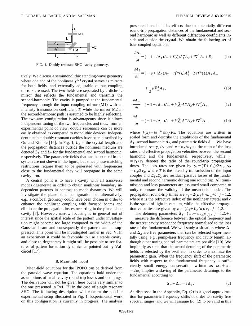
tively. We discuss a semimonolithic standing-wave geometrywhere one end of the nonlinear � (2) crystal serves as mirrorsfor both fields, and externally adjustable output couplingmirrors are used. The two fields are separated by a dichroicmirror that reflects the fundamental and transmits thesecond-harmonic. The cavity is pumped at the fundamentalfrequency through the input coupling mirror �M1� with anintensity transmission coefficient T, while the mirror M2 inthe second-harmonic path is assumed to be highly reflecting.The two-arm configuration is advantageous since it allowsindependent tuning of the two frequencies and thus, from anexperimental point of view, double resonance can be moreeasily obtained as compared to monolithic devices. Indepen-dent tunable doubly resonant cavities have been described byOu and Kimble �16�. In Fig. 1, Lc is the crystal length andthe propagation distances outside the nonlinear medium aredenoted L1 and L2 for the fundamental and second harmonic,respectively. The parametric fields that can be excited in thesystem are not shown in the figure, but since phase-matchingrestrictions require them to be generated with frequenciesclose to the fundamental they will propagate in the samecavity arm.

A central point is to have a cavity with all transversemodes degenerate in order to obtain nonlinear boundary in-dependent patterns in contrast to mode dynamics. We willinvestigate the plane-plane configuration but alternatively,e.g., a confocal geometry could have been chosen in order toenhance the nonlinear coupling with focused beams andeliminate the propagation losses occurring in the plane-planecavity �7�. However, narrow focusing is in general not ofinterest since the spatial scale of the pattern under investiga-tion might become too large compared to the width of theGaussian beam and consequently the pattern can be sup-pressed. This point will be investigated further in Sec. V. Inan experiment it could be favorable to use a stable cavity,and close to degeneracy it might still be possible to see fea-tures of pattern formation dynamics as pointed out by Val-carcel �17�.

B. Mean-field model

Mean-field equations for the IPOPO can be derived fromthe paraxial wave equation. The equations hold under theassumptions of small cavity round-trip losses and detunings.The derivation will not be given here but is very similar tothe one presented in Ref. �7� in the case of singly resonantSHG. The following description will concern the specificexperimental setup illustrated in Fig. 1. Experimental workon this configuration is currently in progress. The analysis

presented here includes effects due to potentially differentround-trip propagation distances of the fundamental and sec-ond harmonic as well as different diffraction coefficients in-side and outside the crystal. We obtain the following set offour coupled equations:

�A1

�t��1�i�1�A1� f ��A1*A2�i�

2 A1�E , �1a�

�A2

�t��i�2�A2�� f *��A1

2�2� f *� � �A�A�

�i

2v�

2 A2 , �1b�

�A�

�t��1�i��A�� f � � �A�*A2�i�

2 A� , �1c�

�A�

�t��1�i��A�� f � � �A�*A2�i�

2 A� , �1d�

where f (x)�ie�ixsin(x)/x. The equations are written inscaled form and describe the amplitudes of the fundamentalA1, second harmonic A2, and parametric fields A� . We haveintroduced �2 /1 and v�v2 /v1 as the ratio of the lossrates and effective propagation velocities between the secondharmonic and the fundamental, respectively, while ��1 /�2 denotes the ratio of the round-trip propagationtimes. The loss rates are given by 1�(T�L1)/2�1 , 2�L2/2�2, where T is the intensity transmission of the inputcoupler and L1 ,L2 are residual passive losses of the funda-mental and second harmonic during one round trip. All trans-mission and loss parameters are assumed small compared tounity to ensure the validity of the mean-field model. Thepropagation round-trip times are � j�2(L j�nLc)/c , j�1,2,where n is the refractive index of the nonlinear crystal and cis the speed of light in vacuum, while the effective propaga-tion velocities are given by v j�(L j�Lc /n)/� j , j�1,2.

The detuning parameters � j�(� j�� j ,c)/1 , j�1,2,� ,� measure the difference between the optical frequency andthe nearest cavity resonance frequency normalized to the lossrate of the fundamental. We will study a situation where �1and �2 are free parameters that can be selected experimen-tally using, e.g., pump-laser frequency and cavity length, al-though other tuning control parameters are possible �10�. Weimplicitly assume that the actual detuning of the parametricfields is selected by the oscillator in order to maximize theparametric gain. When the frequency shift of the parametricfields with respect to the fundamental frequency is suffi-ciently small energy conservation written as ��

�2�1 implies a slaving of the parametric detunings to thefundamental according to

��2�1 . �2�

As discussed in the Appendix, Eq. �2� is a good approxima-tion for parametric frequency shifts of order ten cavity freespectral ranges, and we will assume Eq. �2� to be valid in this

FIG. 1. Doubly resonant SHG cavity geometry.

P. LODAHL, M. BACHE, AND M. SAFFMAN PHYSICAL REVIEW A 63 023815

023815-2

paper. For larger parametric frequency shifts the parametricdetunings may not satisfy Eq. �2�. Analysis of that situationlies outside the scope of the present paper.

In addition to the slaving of the parametric detunings wewill, without loss of generality, assume that �� for thefollowing reason. Making the transformations A�→A�ei t,A�→A�e�i t, leaves Eqs. �1� unchanged apart from renor-malization of the parametric detunings as ��→�� and��→�� . Assume that we have unequal detunings with�� . Then choosing ��/2 equalizes the renormal-ized �� . We will therefore assume that a frequency shift has been applied such that �� and using Eq. �2� thengives ��1, which will be used in the rest of thispaper.

The scaling used in Eqs. �1� is important in order to con-nect to the physical parameters. The electric-field amplitudeshave been defined as A j�2�LcE j

(0)/(1�1�n), j�1,2,� ,� , where E j

(0) is the amplitude of the electric field invacuum and ��1deff /(nc) is the strength of the nonlinearcoupling, with �1 the frequency of the fundamental field andd eff the effective nonlinearity coefficient. The time and spacecoordinates have been scaled according to the transforma-tions 1t→t , (�k11 /v1)r→r, where k1 is the wave num-ber of the fundamental in vacuum. The fundamental pumpfield has been scaled as E�2��LcEpump

(0) /(12�1

2�n), whereEpump

(0) is the physical electric field in vacuum that can bechosen real due to the free choice of the absolute phase. ��T is the input coupling efficiency of the pump field. Fi-nally, ��kLc , �� kLc are the dimensionless phase-mismatch parameters in the second-harmonic and parametricprocesses, respectively, where �k�2k1�k2 and � k�k�

�k��k2.In Eqs. �1� the parametric fields have been assumed to

propagate the same distance and experience the same passivelosses as the fundamental field. This is a very good assump-tion since phase-matching bandwidth restrictions imply thatthe parametric pairs are created with a frequency close to thefundamental. Furthermore, their frequencies will be close toa cavity resonance positioned an integer multiple of the cav-ity free spectral range away from the fundamental resonance.

III. STABILITY ANALYSIS

In this section we analyze the stability of the homoge-neous solutions. The first subsection will concern the casewhere the system is below the parametric oscillation thresh-old where the parametric fields are zero. In this case insta-bilities seen in a pure SHG system are encountered. Further-more, a stability analysis of the vanishing parametricsolutions allows identification of the parametric oscillationthreshold. The second subsection concerns the IPOPO abovethreshold for the parametric process. Exact solutions for theoff-axis emitted parametric fields are derived and their sta-bility is tested leading to secondary instabilities.

A. Ground-state solutions below parametric threshold

Below the parametric threshold, the homogeneous solu-tions for the parametric fields are A�

0 �A�0 �0. The corre-

sponding homogeneous solutions for the fundamental andsecond harmonic can be found from Eqs. �1� as a straight-forward generalization of the expressions given in �5� to in-clude phase-mismatch and different propagation distancesbetween the fundamental and second harmonic. We obtainthe following expressions

� �2� f ��4

2��22

�A10�4�2

��1�2

2��22

�� f ��2�A10�2�1��1

2��A1

0�2�E2, �3a�

�A20��

�� f ��

�2��22

�A10�2. �3b�

A linear stability analysis is performed by perturbing thehomogeneous solutions according to

A1�A10�a1exp��t�ik�•r��b1exp��*t�ik�•r�, �4a�

A2�A20�a2exp��t�ik�•r��b2exp��*t�ik�•r�,

�4b�

A��a�exp� �t�ik�•r��b�exp� �*t�ik�•r�. �4c�

We note that the stability analysis for the parametric fieldsdetermines the threshold for onset of the parametric oscilla-tions. The problem factorizes into two quartic characteristicpolynomials in the two independent eigenvalues � and �

��4�2�1��3�a2�k�2 ��2�a1�k�

2 ��a0�k�2 ��

�� 2�2��1�� k�2 ��1�2�� f � � ��2�A2

0�2�2�0,

�5�

where the coefficients are given by

a0�k�2 ��4�� f ��2�A1

0�2�� f ��2�A10�2�� 1 2�

��2� 22��1� 1

2�� f ��2�A20�2�, �6a�

a1�k�2 ��4�1�� f ��2�A1

0�2�2�1�� 12��2 2

2

�2� f ��2�A20�2, �6b�

a2�k�2 �� f ��2�4��A1

0�2��A20�2��1��4�� 1

2� 22 ,

�6c�

and all the dependence on the transverse wave number k� isin the generalized detuning coefficients

1��1�k�2 , �7a�

2��2�1

2vk�

2 . �7b�

One class of instabilities is obtained by solving Re(�)�0. They appear in pure SHG, where the parametric fields

SPATIOTEMPORAL STRUCTURES IN THE INTERNALLY . . . PHYSICAL REVIEW A 63 023815

023815-3

are not excited, and the four different types of instabilitieswere investigated first by Etrich et al. �4,5� and briefly re-viewed below.

In the case of homogeneous perturbations without anyspatial modulation (k��0) bistability occurs and the thresh-old is obtained by solving a0(k�

2 �0)�0. In the bistabilityregime localized structures can be found numerically. Bysolving ��i�c in the characteristic equation, a Hopf insta-bility is obtained, which implies time oscillating solutionswith a frequency given by

�c�� a1�k�2 �

2�1��. �8�

This phenomenon, known as self-pulsing, was first predictedby Drummond et al. �18�. Transverse instabilities are foundby solving a0(k�

2 )�0 allowing for k� to be different fromzero. The most unstable transverse wave-vector componentkc is located by furthermore requiring �Re(�)/�k��0,which is equivalent to �a0(k�

2 )/�k�2 �0. By differentiating

Eq. �6a� a cubic equation in k�2 is obtained that can be solved

to find kc . Finally, also an oscillatory transverse instabilitycan occur with the oscillation frequency �c given by Eq. �8�and with the transverse wave number and threshold obtainedby solving the equations

�c4�a2�k�

2 ��c2�a0�k�

2 ��0, �9a�

�a2�k�2 �

�k�2

�� a2�k�2 �

a1�k�2 �

�1

1� � �a1�k�2 �

�k�2

�1

�c2

�a0�k�2 �

�k�2

�0.

�9b�

From the expressions in this paragraph the spatial scale kc ,oscillating frequency �c , as well as the threshold amplitudesE ,�A1�,�A2� for the various instabilities can be found. In thispaper we are in particular concerned with how these SHGinstabilities are modified due to the competing parametricprocess in the IPOPO. The detailed analysis of this problemis given in Sec. IV.

A fundamentally different instability is the oscillation ofthe parametric process investigated by substituting �Re�0 inthe characteristic polynomial of Eq. �5� as treated in Ref. �9�.The threshold amplitude for this instability is given by

�A1,p0 �2�

�2��22

�� f �� f � � �� 1 if �1�0

�1��12 if �1�0

�10�

The parametric pairs are emitted off axis with k c��1 for�1�0 and on axis k c�0 for �1�0. A more elaborate de-scription of this parametric instability is given in the nextsection where exact solutions above threshold for the para-metric process are found.

B. Exact solutions above parametric threshold

The exact analytical solutions are homogeneous planewaves for the fundamental and second harmonic, and off-

axis emitted traveling waves for the parametric fields, corre-sponding to the following ansatz

A1�A1 , �11a�

A2�A2 , �11b�

A��A�exp��i� k�•r��t �� . �11c�

After substitution into Eqs. �1�, and using ��1, weobtain

�1�i�1�A1� f ��A1*A2�E , �12a�

��i�2�A2�� f *��A12�2� f *� � �A�A� , �12b�

�1�i�� k�2 ��1��A�� f � � �A2A�* , �12c�

�1�i�� k�2 ��1��A�*� f *� � �A2*A� . �12d�

The existence of nontrivial solutions for the parametric fieldsrequires ��0 and we have �A��A��A�. The ampli-tudes of the exact solutions are obtained by solving

�A1�2��1�E2��2�A�2, �13a�

�A2�2� � k�

2 �

� f � � ��2, �13b�

�A�4��3�A�2��4�1

4

� f ��2

� f � � ��2�A1�4, �13c�

where we have introduced the coefficients

�1�E2�� f � � ��2E2�2 � k�

2 ��1�2�

�� f � � ��2�1��12�� f ��2 � k�

2 �, �14a�

�2�4� f � � ��2� � k�

2 ��cos �� k�2 ��1sin�� k�

2 ��

� f � � ��2�1��12�� f ��2 � k�

2 �,

�14b�

�3�� k�

2 ��cos�� k�2 ��2sin�� k�

2 ��

�� f � � ��2, �14c�

�4� � k�

2 ��2��22�

4�2� f � � ��4, �14d�

and all the dependence on the transverse wave number k�2 is

in the parameters

� k�2 ��1��1� k�

2 �2, �15a�

�� k�2 ��arctan��1� k�

2 �. �15b�


023815-4

These exact solutions above threshold of the parametric pro-cess were stated in Ref. �14� under simplified conditions of

v��1 and equal phase-matching parameters �� . Relax-ing on the latter condition is found to lead to new types ofinstabilities as investigated below.

In order to perform a stability analysis of the exact solu-tions also the phases must be found. We introduce the fol-lowing notation:

A j��A j�ei� A j, �16�

j�1,2,� ,� . It turns out that only the sum of the parametricphases can be calculated from the Eqs. �12�. We will assumesymmetric conditions with � A�

�� A�� A/2. The phases

can be found by solving

� A1�arg��1�i�1��A1�2��i�2��A2�2

�2�� f � � ��A2��A�2ei�( k�2 )� , �17a�

� A2�arg��i�2��A2��2�� f � � ��A�2

�e�i�( k�2 )��2� A1

�� f , �17b�

� A�� A2�� f�� k�

2 �, �17c�

where � f�arg� f (�)� and � f�arg� f ( �)� . Note that the free-dom in choice of the parametric phases implies that theirdifference is subject to a diffusive process �19�. Numericalsimulations in regimes where the exact solutions are stable,support the presence of such a phase diffusive process. It isobserved that different initial noise levels and noise valuesresult in different end results for the parametric phases, al-though the sum of these is in correspondence with the valuecalculated with Eq. �17c�.

Bistability in the parametric solutions occurs when Eq.�13c� has two physical solutions for a given value of E. Itarises when the ground-state solutions A��0 become un-stable through a subcritical bifurcation, and thus correspondsto bistability between the parametric solutions below andabove threshold. This turns out to happen only for negativefundamental detuning where the parametric fields are emittedon axis, k��0. Necessary conditions for the parametric bi-stability to exist include unequal phase mismatch of the twocompeting processes (��) as well as

� f ��2�� f � � ��2

2� f �� f � � ��1�2��1��1

2��2��2�, �18�

which implies �1�2� . The bistability region is E1�E�Ep with the boundary values given by

Ep2�

1��12

�� f � � ��2 � � f ��2�� f � � ��2

� f �� f � � ��

��1��12��2��2

2��2��1�2�� , �19a�

E12�

�� f ��2�� f � � ��2�

�� f �� f � � ��3�1��1

2��2��1�,

�19b�

where Ep is the parametric oscillation threshold. Thus, theIPOPO contains two distinct types of bistabilities that can beattributed to the SHG and OPO processes, respectively.However, while the SHG bistability is found to behave in asimilar way as in a pure SHG system, the parametric bista-bility is found to lead to new effects compared to the exter-nally pumped OPO, as will be explored in Sec. IV B. Studiesof bistability and cavity solitons in the ordinary pumpedOPO have been performed both in the degenerate �20–22�and nondegenerate configurations �3,23–25�.

The exact parametric solutions can be tested by a stabilityanalysis. The solutions are perturbed according to

A j�A j�a jexp ��t�iK•r��b jexp ��*t�iK•r�, �20a�

A��exp��ik�•r�� A��a�exp ��t�iK•r��b�

�exp ��*t�iK•r�� , �20b�

j�1,2. This analysis is similar to the one described in Sec.III A except that it is further complicated by the nonvanish-ing amplitudes of the parametric fields leading to an 8�8matrix problem for computation of the eigenvalues. Equa-tions �11� constitute a continuous family of exact solutionsby varying the wave number k� . However, at threshold k c ,obtained from the parametric threshold analysis, is selected.The numerical analysis indicates that the solution excited atthreshold also prevails further above threshold. The sameconclusion is reached by investigating growth rates abovethreshold that are found to be peaked at k c , and hence we letk�� k c in Eqs. �20�. For �1�0, the direction of the wavevector K introduced in the transverse perturbations becomesimportant. It can be directed either parallel or perpendicularto the wave vector kc of the exact off axis solution, corre-sponding to Eckhaus and zig-zag instabilities, respectively.For �1�0, the parametric fields are emitted on axis andtherefore the direction of K is unimportant. The results ofthis stability analysis are given in the following section.

IV. INSTABILITIES IN THE IPOPO

In this section results from the linear stability analysis arepresented, and the formation of patterns above instabilitythreshold is investigated numerically using a split-step rou-tine previously discussed in Ref. �7�. The results illustratetwo fundamentally different situations. First we demonstratethat the SHG temporal and spatial instabilities can be ob-served also in the presence of the competing parametric pro-cess, which occurs for parameters where the SHG instabilitythresholds are below the parametric threshold. In the oppo-site case, a stability analysis of the exact solutions in Eqs.�13� predicts quenching of the SHG patterns. In certain re-gions, these exact solutions may destabilize through a sec-ondary instability that recently was shown to lead to forma-


023815-5

tion of novel intensity spiral structures �14�. In this sectionother examples of secondary instabilities are given includingparametric bistability and self-pulsing.

In previous work the extra degrees of freedom associatedwith phase mismatch of the conversion processes have notbeen considered. Introducing nonzero but equal phase mis-matches (�� 0) leads to an identical term f (�) in front ofall nonlinear terms in Eqs. �1� which can be scaled away.Hence, �� 0 does not lead to any new physical effectsbut only to an increase in the thresholds for the instabilities.This is in contrast to the singly resonant second-harmonicgeneration �SRSHG� configuration where phase mismatchwas found to be an important tuning parameter �7�. Thisdifference arises since the axial variation of the second-harmonic field in doubly resonsant SHG is averaged out inthe well-established mean-field description, which is not ap-propriate for the second harmonic in SRSHG.

Introducing different phase mismatches for the two � (2)

processes (��) allows independent tuning of the SHG in-stabilities and the parametric threshold, since the former areindependent of � while the latter depend on both � and � .This can, e.g., be used to move the parametric instabilityabove the SHG instabilities in order to avoid undesiredquenching of the pattern formation. Furthermore, it turns outthat new parametric instabilities can arise that are not presentin the equally phase-matched case, as will be described inSec. IV B. However, in an experimental context, it is worthemphasizing that while the phase-matching parameter � forthe SHG process can be controlled, the parametric pairs willbe emitted with frequencies that lower the parametric thresh-old. From Eq. �10� this is seen to lead to ��0, which will beassumed to be the case in this paper. In certain situations thismay be a too simplistic description since also the require-ment of a nearby cavity resonance contributes to the selec-tion of the parametric frequencies, as was discussed exten-sively in Ref. �10�.

Unless otherwise stated, in this section we will assumeideal phase matching �� 0 and equal propagation dis-tances for the fundamental and second harmonic ��v�1.The significance of unequal propagation distances in an ex-perimental context is discussed in Sec. V.

A. SHG instabilities

In the ideally phase-matched case two distinct parameterregions exist depending on the sign of the fundamental de-tuning �1. For positive �1, the parametric instability is low-est in the system and dominates the behavior as demon-strated in Ref. �9�. Here the robustness of the parametricoff-axis solutions was seen numerically and found to lead toquenching of pattern formation. Although the parametricfields are emitted off axis in the cavity, the process is notfound to lead to any spatial intensity modulation since thenondegenerate parametric fields cannot interfere. In additionto the numerical studies, the parametric quenching of SHGinstabilities can be investigated analytically by the stabilityanalysis of the exact parametric solutions as was outlined inSec. III B. The parametric solutions appear always to be

stable both for perturbations parallel and perpendicular to

kc , thus indicating a complete quenching of pattern forma-tion for positive detuning.

Introducing unequal phase mismatches in the competing

processes (��), the parametric threshold may be shiftedabove the SHG thresholds. In this way the SHG instabilitiescan be excited also for �1�0 when using a pump levelbetween the SHG and parametric thresholds. Increasing Eabove the parametric threshold, however, quenching is foundboth in the stability analysis and numerically, and it is againdue to the off-axis emitted parametric fields. Quenching fromthe parametric process thus seems to be a generic property inthe IPOPO for positive fundamental detuning.

For negative fundamental detuning �1�0, parameter re-gions exist where all types of SHG instabilities have lowestthreshold, i.e., they can be excited. Increasing the pumpabove the parametric threshold, the SHG instabilities canprevail in this case leading to the formation of the samemodulated structures also in the parametric fields. An ex-ample of hexagonal structures in all four fields can be foundin Ref. �9�, and furthermore traveling waves have been ob-served. In some cases the SHG instabilities may be changedsubsequently when increasing the pump above the paramet-ric threshold as well. Such an example is described in thenext section.

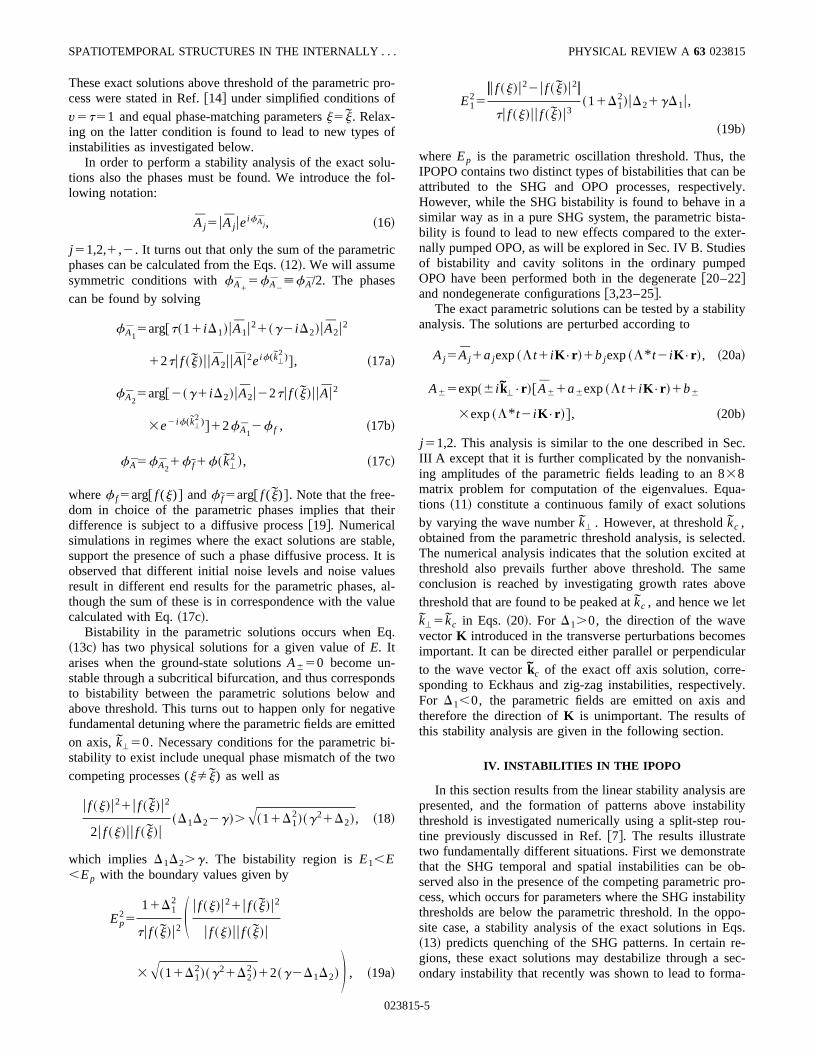
Also the temporal self-pulsing instability can be excitedfor �1�0. This is in contrast to the resonant case treated inRef. �11� where the parametric process was found to quenchself-pulsing completely. The presence of self-pulsing in thedetuned system was suggested in �26� and is here demon-strated explicitly. For the parameters in Fig. 2, close to theself-pulsing threshold (ESP�10.4) a single-frequency oscil-lation is observed with a frequency in agreement with thelinear stability result �c . Further, above threshold, the para-metric threshold (Ep�10.9) is crossed, and self-pulsing inall four fields is obtained as shown in Fig. 2. The primaryfrequency of the oscillations is ��3.39, in reasonable agree-ment with the frequency predicted by the linear stabilitythreshold analysis of �c�3.17. We observe the presence ofperiod doubling as most clearly seen in the fundamentalfield. Such period doubling was previously found in SHG bySavage and Walls �27� to be a prerequisite for chaotic oscil-lations.

The presence of bistability in SHG was extensively dis-cussed in Ref. �4�. In that case cavity solitons can be formedas a consequence of bistability between homogeneous stableand modulationally unstable solutions. This SHG bistabilityis also found in the IPOPO in the case where both the fun-damental and second harmonic have sufficiently large nega-tive detunings. In this region, excitation of cavity solitons inall four fields is possible but will not be discussed furtherhere.

B. Secondary parametric instabilities

Also for negative fundamental detuning the parametricthreshold can be the lowest instability in the system for cer-tain parameters. Hence, the exact parametric solution in Eqs.�11� can be excited, where in that case the parametric fields


023815-6

are emitted on axis with k��0. These solutions can becomeunstable when increasing E due to the presence of secondaryinstabilities in the system. This is in contrast to the off-axissolutions discussed in the previous section that were alwayslinearly stable. Spatiotemporal pattern formation from thissecondary instability was investigated in Ref. �14�. There theformation of traveling roll patterns was observed that coulddestabilize further to form intensity spiral structures consti-tuting a novel type of nonlinear phenomenon in optics.

When the parametric threshold is above an SHG patternthreshold the assumption of spatially homogeneous funda-mental and second-harmonic fields may not be accurate.However, if the modulation from the SHG instability is weakthe ansatz given by Eqs. �11� may still be a reasonable ap-proximation. This allows an analysis of the effect of theparametric process, also in this case, as discussed in the fol-lowing.

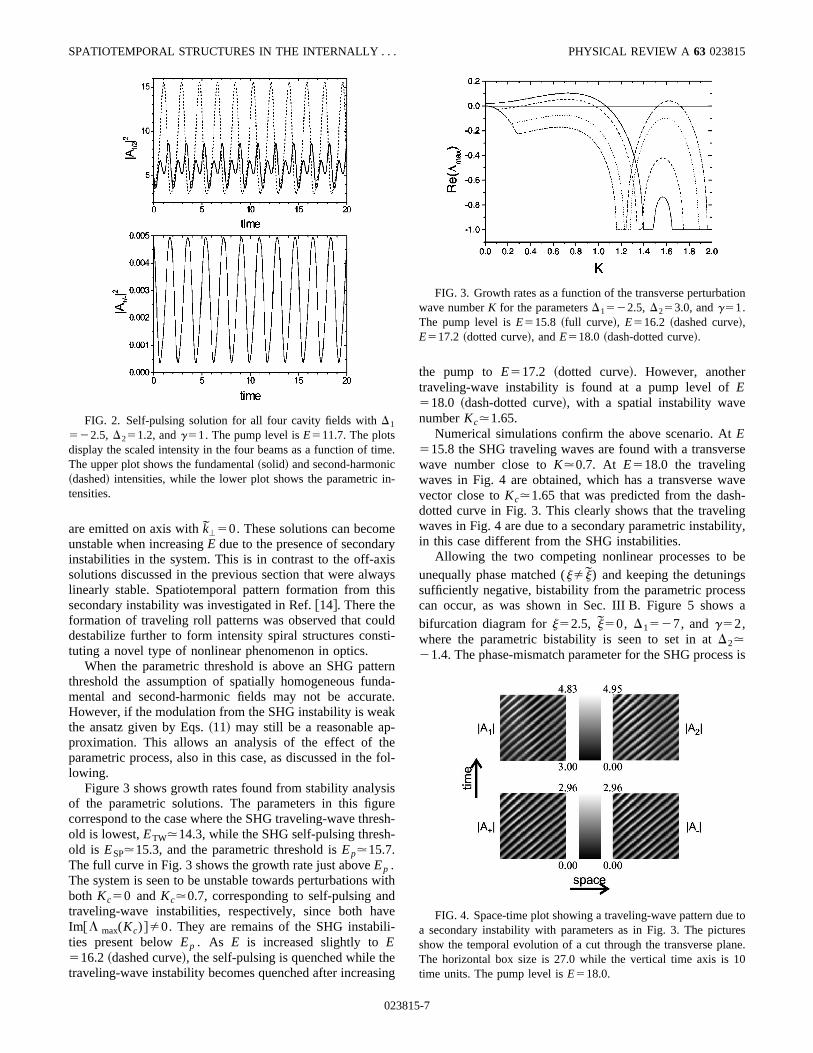
Figure 3 shows growth rates found from stability analysisof the parametric solutions. The parameters in this figurecorrespond to the case where the SHG traveling-wave thresh-old is lowest, ETW�14.3, while the SHG self-pulsing thresh-old is ESP�15.3, and the parametric threshold is Ep�15.7.The full curve in Fig. 3 shows the growth rate just above Ep .The system is seen to be unstable towards perturbations withboth Kc�0 and Kc�0.7, corresponding to self-pulsing andtraveling-wave instabilities, respectively, since both haveIm�� max(Kc)��0. They are remains of the SHG instabili-ties present below Ep . As E is increased slightly to E�16.2 �dashed curve�, the self-pulsing is quenched while thetraveling-wave instability becomes quenched after increasing

the pump to E�17.2 �dotted curve�. However, anothertraveling-wave instability is found at a pump level of E�18.0 �dash-dotted curve�, with a spatial instability wavenumber Kc�1.65.

Numerical simulations confirm the above scenario. At E�15.8 the SHG traveling waves are found with a transversewave number close to K�0.7. At E�18.0 the travelingwaves in Fig. 4 are obtained, which has a transverse wavevector close to Kc�1.65 that was predicted from the dash-dotted curve in Fig. 3. This clearly shows that the travelingwaves in Fig. 4 are due to a secondary parametric instability,in this case different from the SHG instabilities.

Allowing the two competing nonlinear processes to beunequally phase matched (��) and keeping the detuningssufficiently negative, bistability from the parametric processcan occur, as was shown in Sec. III B. Figure 5 shows abifurcation diagram for ��2.5, ��0, �1��7, and �2,where the parametric bistability is seen to set in at �2��1.4. The phase-mismatch parameter for the SHG process is

FIG. 2. Self-pulsing solution for all four cavity fields with �1

��2.5, �2�1.2, and �1. The pump level is E�11.7. The plotsdisplay the scaled intensity in the four beams as a function of time.The upper plot shows the fundamental �solid� and second-harmonic�dashed� intensities, while the lower plot shows the parametric in-tensities.

FIG. 3. Growth rates as a function of the transverse perturbationwave number K for the parameters �1��2.5, �2�3.0, and �1.The pump level is E�15.8 �full curve�, E�16.2 �dashed curve�,E�17.2 �dotted curve�, and E�18.0 �dash-dotted curve�.

FIG. 4. Space-time plot showing a traveling-wave pattern due toa secondary instability with parameters as in Fig. 3. The picturesshow the temporal evolution of a cut through the transverse plane.The horizontal box size is 27.0 while the vertical time axis is 10time units. The pump level is E�18.0.


023815-7

chosen sufficiently large such that the parametric threshold isbelow the SHG thresholds. For a fixed value of the second-harmonic detuning, �2��4, the lower plot in Fig. 6 showsthe characteristic bistability curve of the intracavity paramet-ric intensity as a function of the pump E. At the oscillationthreshold (Ep�66.2) the ground-state parametric solution,A��0 �solid curve�, bifurcates subcritically into an unstablebranch �dotted curve�. This middle branch is linearly un-stable and using Eq. �19b� is found to bifurcate at E1

�59.5 into a modulationally unstable upper branch �dashedcurve�. The corresponding bistability curves for the funda-mental and second harmonic are also displayed in Fig. 6. Thefundamental bistability curve is seen to be inverted such thatthe modulational branch is below the homogeneous solution.The second harmonic, however, is clamped at a constantvalue above the parametric threshold as is also seen from Eq.�13b�, which follows from the exact balancing of the twocompeting frequency conversion processes in steady state.This clamping was observed in Ref. �28�.

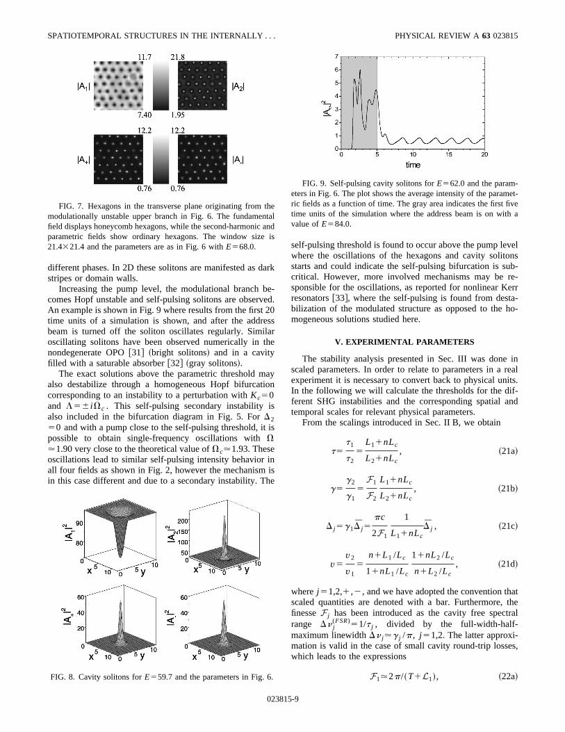
The inverted bistability curve for the fundamental fieldpromises formation of spatial structures consisting of holesin the homogeneous background. An example of such a hon-eycomb structure in the fundamental is shown in Fig. 7 forE�68.0 corresponding to a pump level above the bistabilityregion. The modulated structures in the three other fields areordinary hexagons in agreement with expectations from Fig.6. The average intensities are found to oscillate in time dueto a self-pulsing instability in the system, which could not bepredicted directly from the stability analysis.

Bistability between a homogeneous stable ground stateand a modulationally unstable upper state can lead to forma-tion of localized structures, also called cavity solitons. Un-like temporal solitons in, e.g., fiber optics, these solitons area result of a careful preparation of the system. Using a local-ized address beam a small part of the system is set in themodulationally unstable upper state, while the rest of thesystem is maintained at the homogeneous background level.These states must be connected to each other by transitionalkink type waves, also called switching waves �29�, that canlock mutually to form solitonlike structures.

In order to investigate the formation of cavity solitonsnumerically, the system was prepared as follows. The local-ized Gaussian address beam had a pump value well abovethe upper limit of the bistable area. After 5 time units theaddress beam was switched off and the evolution of thefields was followed. For a pump value close to the bistablelower limit, E�59.7, it is possible to obtain stable cavitysolitons, where an example is shown in Fig. 8. The funda-mental soliton is a so-called gray soliton, since it constitutesa localized hole in the homogeneous background as a conse-quence of the inverted fundamental bistability curve. Thesecond harmonic and parametric solitons are all bright soli-tons, and generally the solitons may be seen as residuals ofthe modulational structure of the upper branch, which in thiscase are the hexagons shown in Fig. 7. Note that cavity soli-tons may also be observed by pumping well above the bista-bility limits to obtain the hexagonal patterns in Fig. 7, andthen slowly decreasing the pump level to enter the bistablearea. The appearance of two-dimensional �2D� gray solitonsis, to our knowledge, a new phenomenon in � (2) cavity in-teractions. However, 1D dark solitons have been reported inthe OPO �30� due to a different mechanism based on thecoexistence of two parametric homogeneous solutions with

FIG. 5. Bifurcation diagram for �1��7, �2, ��2.5, and ��0. The bold-solid line is the SHG transverse threshold while thebold-dashed lines are limit points of the SHG bistable area. Thethin-solid line is the parametric threshold, the thin-dashed lines arelimits of the parametric bistable area. Finally, the thin-dotted line isthe self-pulsing secondary instability.

FIG. 6. Intracavity fields as a function of E. The full �dashed�curves are the solutions below �above� the parametric thresholdwhile the dotted curves are linearly unstable homogeneousbranches. The parameters are as in Fig. 5, and with �2��4.


023815-8

different phases. In 2D these solitons are manifested as darkstripes or domain walls.

Increasing the pump level, the modulational branch be-comes Hopf unstable and self-pulsing solitons are observed.An example is shown in Fig. 9 where results from the first 20time units of a simulation is shown, and after the addressbeam is turned off the soliton oscillates regularly. Similaroscillating solitons have been observed numerically in thenondegenerate OPO �31� �bright solitons� and in a cavityfilled with a saturable absorber �32� �gray solitons�.

The exact solutions above the parametric threshold mayalso destabilize through a homogeneous Hopf bifurcationcorresponding to an instability to a perturbation with Kc�0and ��i�c . This self-pulsing secondary instability isalso included in the bifurcation diagram in Fig. 5. For �2�0 and with a pump close to the self-pulsing threshold, it ispossible to obtain single-frequency oscillations with ��1.90 very close to the theoretical value of �c�1.93. Theseoscillations lead to similar self-pulsing intensity behavior inall four fields as shown in Fig. 2, however the mechanism isin this case different and due to a secondary instability. The

self-pulsing threshold is found to occur above the pump levelwhere the oscillations of the hexagons and cavity solitonsstarts and could indicate the self-pulsing bifurcation is sub-critical. However, more involved mechanisms may be re-sponsible for the oscillations, as reported for nonlinear Kerrresonators �33�, where the self-pulsing is found from desta-bilization of the modulated structure as opposed to the ho-mogeneous solutions studied here.

V. EXPERIMENTAL PARAMETERS

The stability analysis presented in Sec. III was done inscaled parameters. In order to relate to parameters in a realexperiment it is necessary to convert back to physical units.In the following we will calculate the thresholds for the dif-ferent SHG instabilities and the corresponding spatial andtemporal scales for relevant physical parameters.

From the scalings introduced in Sec. II B, we obtain

��1

�2

�L1�nLc

L2�nLc

, �21a�

�2

1

�F1

F2

L1�nLc

L2�nLc

, �21b�

� j�1� j��c

2F1

1

L1�nLc

� j , �21c�

v�v2

v1

�n�L1 /Lc

1�nL1 /Lc

1�nL2 /Lc

n�L2 /Lc

, �21d�

where j�1,2,� ,� , and we have adopted the convention thatscaled quantities are denoted with a bar. Furthermore, thefinesse Fj has been introduced as the cavity free spectralrange �� j

(FSR)�1/� j , divided by the full-width-half-maximum linewidth �� j� j /� , j�1,2. The latter approxi-mation is valid in the case of small cavity round-trip losses,which leads to the expressions

F1�2�/�T�L1�, �22a�

FIG. 7. Hexagons in the transverse plane originating from themodulationally unstable upper branch in Fig. 6. The fundamentalfield displays honeycomb hexagons, while the second-harmonic andparametric fields show ordinary hexagons. The window size is21.4�21.4 and the parameters are as in Fig. 6 with E�68.0.

FIG. 8. Cavity solitons for E�59.7 and the parameters in Fig. 6.

FIG. 9. Self-pulsing cavity solitons for E�62.0 and the param-eters in Fig. 6. The plot shows the average intensity of the paramet-ric fields as a function of time. The gray area indicates the first fivetime units of the simulation where the address beam is on with avalue of E�84.0.


023815-9

F2�2�/L2 . �22b�

The intensity of the fundamental pump field is given by

Ipump��0c

2�Epump

(0) �2��0cn3�2�2

32deff2 Lc

2

1

TF14

E2, �23�

where �0 is the vacuum permittivity and � is the fundamen-tal wavelength.

We consider an experiment consisting of a 1-cm longLiNbO3 crystal placed in a cavity with L1�L2�1 cm.LiNbO3 can be noncritically phase matched for frequencydoubling at the Nd:YAG wavelength ��1064 nm, wherethe effective nonlinear coefficient is deff�4.7 pm/V and therefractive index is n�2.2 �34�. Furthermore, the finesse ofthe fundamental and second-harmonic cavities are assumedto be F1�F2�100 and the fundamental input coupler trans-mission T�3%. From these numbers the cavity linewidthfor the fundamental and second harmonic are calculated tobe ��1��2�47 MHz. In Fig. 10 the pump intensity nec-essary to reach threshold for the different instabilities in thesystem is plotted as a function of the detuning of the secondharmonic while the fundamental detuning is fixed at �1�

�368 MHz, which corresponds to a scaled detuning �1��2.5. A typical threshold value is about 0.1 kW/mm2,which should be easily accessible with a pulsed Nd:YAGlaser. For comparison, experiments on spatial soliton forma-tion in � (2) propagation geometries require on the order of1 GW/mm2 �35�.

The spatial scale of the transverse structure kc and theself-pulsing frequency �c can be transformed into physicalunits as

kc��k11

v1

k c��2n�2

�F1

1

Lc�nL1

k c , �24a�

�c�1�c��c

2F1

1

L1�nLc

�c . �24b�

Defining lc�2�/kc as the scale of the spatial modulation, itis favorable to have lc small since this allows more narrow

focusing in the crystal and thus higher intensities. In order toobserve pattern formation in an experiment a minimum re-quirement is that the width of the Gaussian beam is largerthan the pattern scale, i.e., 2w0�lc , where w0 is the beamradius at the waist. We observe from Eq. �24a� that to obtaina small spatial scale requires a short cavity. It is especiallyimportant to minimize the propagation distance outside thecrystal since the beam diffracts less in a medium with areduction factor given by the refractive index. The spatialscales for the stationary and oscillatory transverse structuresare plotted in Fig. 11 as a function of the scaled second-harmonic detuning �2 for different values of the fundamen-tal finesse. The scaled detuning is used in order to relate thedetunings of cavities with different values of the fundamen-tal finesse. All other parameters are as described above andin particular �1��2.5 for all curves. The typical spatialscale is seen to be about 1 mm.

In Fig. 12 the self-pulsing frequency �c is plotted as afunction of the second-harmonic detuning for the same valueof the fundamental detuning as in Fig. 10. The typical self-pulsing frequency is found to range from about 300 MHz to1 GHz, and is not changed considerably when varying thefundamental detuning.

Finally, the extra degrees of freedom contained in theratios of the round-trip times � and the propagation velocitiesv should be considered. From an experimental point of view

FIG. 10. The threshold pump intensity for the different instabili-ties in the system. The parameters are specified in the text. Thincurve: parametric instability; bold curve: stationary transverse insta-bility; thin-dashed curve: self-pulsing instability; bold-dashedcurve: oscillatory transverse instability.

FIG. 11. Spatial scale of the transverse instability displayed asfunction of the scaled second harmonic detuning. The bold and thincurves are the stationary and oscillatory instabilities, respectively.The full, dashed and dotted curves correspond to a fundamentalfinesse of 50, 100, and 150, respectively. F2�100.

FIG. 12. Self-pulsing frequency �c plotted as function of thesecond-harmonic detuning for �1��368 MHz. The thin and boldcurves correspond to the spatially homogenous and modulated in-stabilities, respectively.


023815-10

they may appear to be important since they can be used asconvenient tuning parameters. Varying � by changing thepropagation distances of the fundamental or the second har-monic is seen to be a way to change the loss-rate ratio ,which is more easily accessible experimentally than bychanging the respective propagation losses of the two fields.The parameter v is found to influence only the diffractionterms and can therefore be used to tune the spatial period ofthe modulated structure. This may be convenient in order tooperate in a regime where the spatial period is small suchthat a more narrow Gaussian pump beam can be used toenhance the nonlinearity. One way of changing v is to varythe length of the second-harmonic arm L2, while keeping thelength of the fundamental arm L1 fixed. Figure 13 shows thevariation of the spatial scale with L2. It is observed thatsubstantial tuning of the spatial scale is possible and in gen-eral a small value of L2 is desirable.

VI. CONCLUSIONS

This paper concerned pattern formation in doubly reso-nant SHG in a two-armed cavity configuration of relevancefor experimental realizations. As pointed out in previouswork the presence of a competing parametric process mayinfluence the pattern formation of the system decisively. Aset of coupled cavity mean-field equations generalized to in-clude also unequal phase mismatch for the two competingprocesses as well as different propagation distances for thefundamental and second harmonic, was presented to modelthis system. The instabilities were divided into SHG andparametric instabilities, according to the relative position ofthe SHG instability thresholds to the parametric instabilitythreshold. The parametric instability could be studied in de-tail by deriving exact analytical solutions that were found toimply complete quenching of spatially modulated intensitystructures for positive fundamental detuning. For negativefundamental detuning, however, the parametric solutionscould destabilize leading to new phenomena. Here we haveconsidered parametric bistability and self-pulsing that onlywere found for unequal phase mismatch of the two compet-ing processes. These instabilities were found to lead to for-mation of a honeycomb pattern and gray solitons. Finally,

numerical estimates of the threshold intensity and spatiotem-poral scales for the instabilities were given for realistic ex-perimental parameters.

APPENDIX: DETUNING OF THE PARAMETRICFIELDS

In this appendix we discuss the relationship between thedetuning of the fundamental and parametric fields. Energyconservation requires

2�1�� , �A1�

where � j is the angular frequency of field j. In a monolithicresonator containing a dispersive crystal there are a set ofresonances at vacuum wavelengths �p satisfying

2Lcnp

�p

�p , �A2�

where Lc is the crystal length, p is an integer, and np�n(�p) is the crystal’s index of refraction at �p . For sim-plicity we have neglected the distance L1 in Fig. 1. Thecorresponding set of resonant frequencies is

�p�2�c

�p

�p�c

Lcnp

. �A3�

Define detunings as j�� j��p j, j�1,� ,� . Then Eq.

�A1� implies

2�p1��p�

��p�� 2 1 . �A4�

Assuming that the parametric fields are emitted symmetri-cally, we have �p�

��p1�m , where m is an integer labelingthe axial mode the parametric fields are nearly resonant with.Hence, the left-hand side of �A4� can be written as

lhs�2�c

�p1

� 2�np1

np�

�np1

np�

�m

p1� np1

np�

�np1

np�

� � . �A5�

Converting to normalized detunings using the same scalingsas in Eqs. �1� then gives

��2�1�8�np1

Lc

�p1

1

T�L1

�� 2�np1

np�

�np1

np�

�m

p1� np1

np�

�np1

np�

� � .

�A6�

When m�0, np��np�

�np1and ��2�1�0. At fi-

nite m this relation is only approximate. As an example,consider LiNbO3 at room temperature, Lc�1 cm, T�L1�0.03, �p1

�1.06 �m, and m�20 �corresponding to awavelength separation between the parametric beams ofabout 1 nm�. Equation �A6� then gives ��2�1�

FIG. 13. The spatial scale of the transverse instability as a func-tion of the length of the second harmonic arm L2. The lengths of thefundamental arm are L1�10 mm �solid�, L1�20 mm �dashed�,and L1�50 mm �dotted�. The parameters are as in Fig. 10 and with

�2��1.5.


023815-11

�0.1, where the refractive indices have been calculated us-ing the Sellmeier equations given in Ref. �34�. In practice theaxial mode shift m, and the selected detuning of the paramet-ric fields from the nearest cavity resonances, depend on theinteraction of the phase mismatch of the fundamental and the

cavity tuning in a rather complicated way �10�. Thus eventhough the fundamental is close to phase matching there maybe a large shift of the parametric frequencies. Analysis ofthat situation, which implies arbitrary parametric detunings,is not included in this paper.

�1� G.-L. Oppo, M. Brambilla, and L.A. Lugiato, Phys. Rev. A 49,2028 �1994�; G.-L. Oppo, M. Brambilla, D. Camesasca, A.Gatti, and L.A. Lugiato, J. Mod. Opt. 41, 1151 �1994�.

�2� K. Staliunas, J. Mod. Opt. 42, 1261 �1995�.�3� S. Longhi, Phys. Rev. A 53, 4488 �1996�.�4� C. Etrich, U. Peschel, and F. Lederer, Phys. Rev. Lett. 79,

2454 �1997�.�5� C. Etrich, U. Peschel, and F. Lederer, Phys. Rev. E 56, 4803

�1997�.�6� S. Longhi, Phys. Rev. E 59, R24 �1999�; Phys. Rev. A 59,

4021 �1999�.�7� P. Lodahl and M. Saffman, Phys. Rev. A 60, 3251 �1999�.�8� P. Lodahl and M. Saffman, Opt. Commun. 184, 493 �2000�.�9� P. Lodahl, M. Bache, and M. Saffman, Opt. Lett. 25, 654

�2000�.�10� S. Schiller and R.L. Byer, J. Opt. Soc. Am. B 10, 1696 �1993�;

S. Schiller, G. Breitenbach, R. Paschotta, and J. Mlynek, Appl.Phys. Lett. 68, 3374 �1996�.

�11� M.A.M. Marte, Phys. Rev. A 49, R3166 �1994�.�12� M.A.M. Marte, Phys. Rev. Lett. 74, 4815 �1995�.�13� A.G. White, P.K. Lam, M.S. Taubman, M.A.M. Marte, S.

Schiller, D.E. McClelland, and H.-A. Bachor, Phys. Rev. A 55,4511 �1997�.

�14� P. Lodahl, M. Bache, and M. Saffman, Phys. Rev. Lett. 85,4506 �2000�.

�15� M. Vaupel, A. Maıtre, and C. Fabre, Phys. Rev. Lett. 83, 5278�1999�.

�16� Z.Y. Ou and H.J. Kimble, Opt. Lett. 18, 1053 �1993�.�17� G.J. de Valcarcel, Phys. Rev. A 56, 1542 �1997�.�18� K.J. McNeil, P.D. Drummond, and D.F. Walls, Opt. Commun.

27, 292 �1978�; P.D. Drummond, K.J. McNeil, and D.F. Walls,Opt. Acta 27, 321 �1980�.

�19� C. Fabre and S. Reynaud, in Fundamental Systems in QuantumOptics, edited by J. Dalibard, J.M. Raimond, and J. Zinn-Justin�Elsevier Science, Amsterdam, 1992�.

�20� K. Staliunas and V.J. Sanchez-Morcillo, Opt. Commun. 139,306 �1997�.

�21� S. Longhi, Phys. Scr. 56, 611 �1997�.�22� D.V. Skryabin and W.J. Firth, Opt. Lett. 24, 1056 �1999�.�23� S. Longhi, Opt. Commun. 149, 335 �1998�.�24� V.J. Sanchez-Morcillo, E. Roldan, G.J. de Valcarcel, and K.

Staliunas, Phys. Rev. A 56, 3237 �1997�.�25� D.V. Skryabin, A.R. Champneys, and W.J. Firth, Phys. Rev.

Lett. 84, 463 �2000�.�26� A. Eschmann and M.A.M. Marte, Quantum Semiclassic. Opt.

9, 247 �1997�.�27� C.M. Savage and D.F. Walls, Opt. Acta 30, 557 �1983�.�28� K. Schneider and S. Schiller, Opt. Lett. 22, 363 �1997�.�29� N.N. Rosanov and G.V. Khodora, J. Opt. Soc. Am. B 7, 1057

�1990�.�30� S. Trillo, M. Haelterman, and A. Sheppard, Opt. Lett. 22, 970

�1997�.�31� G.J. de Valcarcel, E. Roldan, and K. Staliunas, Opt. Commun.

181, 207 �2000�.�32� D. Michaelis, U. Peschel, and F. Lederer, Opt. Lett. 23, 1814

�1998�.�33� M. Hoyuelos, P. Colet, M. San Miguel, and D. Walgraef, Phys.

Rev. E 58, 2992 �1998�.�34� V.G. Dmitriev, G.G. Gurzadyan, and D.N. Nikogosyan: Hand-

book of Nonlinear Optical Crystals �Springer-Verlag, NewYork, 1997�.

�35� W.E. Torruellas, Z. Wang, D.J. Hagan, E.W. VanStryland, G.I.Stegeman, L. Torner, and C.R. Menyuk, Phys. Rev. Lett. 74,5036 �1995�.


023815-12

Spatiotemporal structures in the internally pumped optical parametric oscillator

Documents

Transcript of Spatiotemporal structures in the internally pumped optical parametric oscillator