Spatio-Temporal Simulation of the Field-Scale Evolution of Organic Carbonover the Landscape

C. Walter,* R. A. Viscarra Rossel, and A. B. McBratney

ABSTRACT and biological condition of soil (Oades, 1993; Stevenson,1994). To maintain SOC in agricultural fields, we needThe spatial or temporal variability of soil has been extensivelyto consider its local and global evolution. With respectconsidered in the literature using either experimental or modeling

approaches. However, only a few studies integrate both spatial and to the latter, global warming and the potential releasetemporal dimensions. The aim of this paper is to present a method or sequestration of C into or from the atmosphere mustfor field-scale simulations of the spatio-temporal evolution of topsoil be considered. Intermediate spatial scales such as varia-organic C (OC) at the landscape scale over a few decades and under tions along slopes are also important as they contributedifferent management strategies. A virtual landscape with characteris-

to soil diversity, which impacts biodiversity (Ibanez ettics matching part of Brittany (France) was considered for the study.al., 1995).Stochastic simulations and regression analysis were used to simulate

The spatial or temporal variability of soil organic mat-spatial fields with known spatial structures: short-range, medium-range, and long-range variability. These were then combined using an ter has been extensively considered by experimental oradditive model of regionalization. Agricultural land use was simulated modeling approaches (Balabane and Balesdent, 1995;considering four different land uses: permanent pasture, temporary Bernoux et al., 1998; Smith et al., 1997; Six et al., 1999;pasture, annual cereal crops, and maize (Zea mays L.). Land use Collins et al., 2000; Arrouays et al., 2001), but only fewevolution over time was simulated using transition matrices. Evolution

studies integrate both spatial and temporal dimensionsof soil organic matter was estimated each year for each pixel through(Jolivet et al., 1997; Papritz and Webster, 1995). Thea rudimentary balance model that accounts for land use and theones that do, neglect short- and medium-range spatialinfluence of soil waterlogging on mineralization rates. This spatio-

temporal simulation approach at the landscape level allowed the simu- variability and consider only mean values (Smith et al.,lation of several scales of soil variability including within-field variabil- 1997; Nieder and Richter, 2000). Thus the impact ofity. Spatial variability decreased drastically over time when only the management strategies on soil, at both the field andinfluence of land use was considered. This effect on soil variability landscape scales, cannot be adequately evaluated. Fur-over the landscape may have implications for site-specific soil manage-

thermore, the design of soil monitoring networks cannotment and precision agriculture. The presence of redoximorphic condi-be tested a priori for their ability to detect the evolutiontions was found to maintain soil spatial variability.of selected soil properties in a given region (Mol etal., 1998).

The validation of temporal modeling that also com-In recent years, soil quality has received much lessbines several spatial scales of variation is very difficult,attention than water quality, especially in regionsif not impossible, on real soil landscapes. One reasonwhere soil degradation and reduced yields have notfor this is the trade-off between sampling density andmanifested themselves. Identifying soil degradation isthe cost of the survey, that is, soil sampling is eitherusually based on observations of trends from historicaltoo sparse or too expensive. Recent developments insoil data and on comparisons of projections that aresimulation techniques (Hauhs, 1990; Philip, 1991; Goo-made over time. In regions with intensive farming sys-

tems, concerns about reductions in organic matter, ni- vaerts, 2000) enable alternative approaches that allowtrate leaching, accumulation of P, or contamination by the creation of virtual soil landscapes with inherent spa-trace elements are much more justified by examining tial structures that are similar to those observed in real-trends than by present indicators (Coppenet et al., 1993, ity. The virtual landscape can then be modified overWalter et al., 1997). The assessment of soil quality needs time considering different management scenarios andthe spatial prediction of soil attributes under different the evolution of the spatial structures described.management practices and over many decades. In doing The aim of this paper is to present a method for field-so, both field and landscape scales should be considered. scale simulations of the spatio-temporal evolution of

Soil organic C (SOC) is of particular interest in agri- topsoil OC at the landscape scale over a few decadesculture because of its role in biochemical transforma- and under different management strategies. The aim istions that occur in soil (Baldock and Nelson, 2000). It achieved by: (i) creating a virtual landscape; (ii) simulat-is also of crucial consequence to the chemical, physical, ing an initial SOC content distribution with respect to

the observed spatial structures; and (iii) modeling theC. Walter, ENSA-INRA Rennes, 65 rue de St Brieuc, CS 84215, 35042 temporal evolution of SOC over four decades, consider-Rennes, France; R.A. Viscarra Rossel, and A.B. McBratney, Faculty ing land use, the influences of soil waterlogging, andof Agriculture, Food and Natural Resources, The University of Syd- their combined effect.ney, NSW 2006, Australia. Received 26 Feb. 2002. *Correspondingauthor (cwalter@roazhon.inra.fr).

Abbreviations: DEM, digital elevation model; HI, hydromorphic in-Published in Soil Sci. Soc. Am. J. 67:1477–1486 (2003). Soil Science Society of America dex; OC, organic C; RF, random function; SOC, soil organic C; VQT,

variance quadtree algorithm.677 S. Segoe Rd., Madison, WI 53711 USA

1477

1478 SOIL SCI. SOC. AM. J., VOL. 67, SEPTEMBER–OCTOBER 2003

Fig. 1. Framework of the combination of stochastic and deterministic approaches to simulate the initial spatial field of soil organic C contentover the landscape. DEM, digital elevation model; HI, hydromorphic index; OC, organic C.

The Landscape of the Study AreaMATERIALS AND METHODSFor each cell in the study area, the altitude was availableThe overall methodology is shown in Fig. 1. The study area

from a DEM (Fig. 2a). Landscape attributes such as slope,consists of a virtual, 15 by 15 km, agricultural landscape withsurface drainage (Wilson and Gallant, 2000), and a soil hydro-characteristics matching part of Brittany in north-west France.morphic or redoximorphic index (HI) (Chaplot et al., 2000)This area was represented by 90 600 pixels, each being 50 byderived from topographic attributes, were calculated for50 m in size.each cell.

The Initial StateSimulations of Land Use and Field Sizes in the Study AreaWe chose a small subregion of Brittany, for which we had

a detailed digital elevation model (DEM) at an x,y resolution The land use types considered were: (i) permanent pastures(P), (ii) temporary pastures (T), (iii) cereals (C), and (iv)of 50 m and a z resolution of �1 m. Within this subregion,

we had some information on field sizes, on land use and its maize (M). Initially, land use was attributed to each field indefined proportions that were representative of agriculturalchange, and general relationships between soil and topogra-

phy. Thus, we could ascertain certain landscape parameters land use in Brittany in the 1960s. That is, roughly equal propor-tions of permanent and temporary pastures and cereals (ap-such as topography and field sizes before simulation.

WALTER ET AL.: SPATIO-TEMPORAL SIMULATION OF ORGANIC CARBON 1479

Fig. 2. (a) Topography of the virtual study area and (b) initial land use under (P ) long-term pastures; (T ) short-term pastures; (C ) cereals and(M ) maize. Simulations of land use was conducted over 4500 virtual fields.

proximately 30–40%) and a much smaller proportion of maize details, the Cholesky decomposition method is described inCressie (1991). Second, sequential Gaussian simulations offields (approximately 5%).

An adaptation of the variance quadtree algorithm (VQT) the SOC content over the landscape were made onto the finer50-m grid. These simulations, conditioned on the 300-m grid(McBratney et al., 1999) was used to define field sizes over

the study area. The VQT algorithm was developed by McBrat- data resulting from the previous simulations, were made toreproduce the short- and long-range RF models onto a 50-mney et al. (1999) to maximize the efficiency of a sampling

scheme while ensuring that the variability of the sampling grid. Such simulations can produce an infinite number of real-izations that reproduce the global statistics (histogram andarea is characterized effectively. The authors designed the

approach to sample sparsely where variation is low, and more semivariogram), thus it may be important to note that thereis not a unique solution. In this instance, we used a singleintensively where variation is large. In this case, the algorithm

provided us with a means of partitioning the variance of the realization of the process for the study. Goovaerts (1997)and Deutsch and Journel (1998) provide the details of theDEM, thus permitting the allocation of smaller virtual fields

to areas of more variable topography (steeper slopes) and sequential Gaussian simulation algorithm used.Deterministic Derivation of the Medium-Range Spatialconversely, larger virtual fields to areas of more homogeneous

topography (Fig. 2b). Pattern. The medium-range spatial field was derived froma linear model that describes the impact of redoximorphicconditions (measured by the HI) on the soil’s OC contentSimulations of Soil Organic Carbon(Fig. 3c). The relationship was derived from experimentalAt Different Spatial Scalesdata at different landscape positions (Chaplot et al., 2001). A

A combination of stochastic and deterministic approaches semivariogram of the SOC estimates was also produced.was used to simulate the initial state of SOC in the study area Combination of the Spatial Fields Characterizing the Dif-(Fig. 1). Semivariograms were used to describe the spatial ferent Spatial Scales. To derive a permissible description ofvariability of SOC at the short- and long-range scales and the overall spatial variability in the study area, the two randoma deterministic model that relates variations in SOC to soil functions that describe the short- and long-range variabilitywaterlogging was used to derive the medium range structure. of SOC were combined with the medium-range spatial field

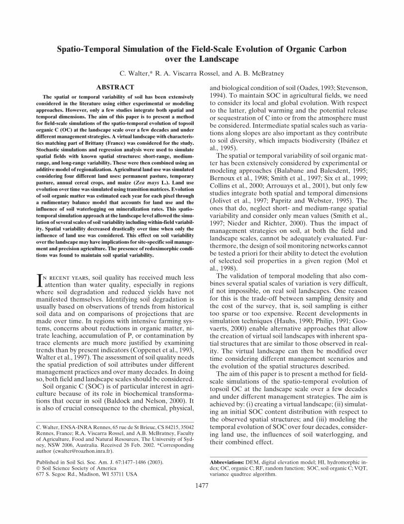
Short- and Long-Range Spatial Variability of Organic Car- using a linear model of regionalization (Goovaerts, 1997)bon. A semivariogram characterizing the short-range variabil- (Fig. 1). The combined spatial field S(x) was derived from aity of SOC in the study area was derived using 360 samples linear combination of the two independent RFs [Yi(x)] andfrom a nested survey conducted in the south of Brittany (Wal- the deterministic spatial field Yi(x), so that:ter, 1990) (Fig. 3a). Similarly, a semivariogram characterizingthe long-range variability in SOC (i.e., that occurring at a S(x) � �

3

i�1

aiYi(x) [2]regional scale, between 3000 and 35 000 m�) was derived using40 000 samples from a regional study conducted in Brittany by

where each RF and spatial field Yi(x) has zero mean andWalter et al. (1997) (Fig. 3e).semivariogram �i(h). Therefore, the combined permissibleSimulations of the Short- and Long-Range Spatial Patterns.semivariogram was described as a linear combination of eachGeostatistical simulations of SOC at these scales were con-of the three semivariogram models �i(h), so that:ducted over the landscape to derive respective random func-

tion (RF) models that may be representative of the study area�(h) � �

3

i�1

bi�i(h) [3](Fig. 3). The simulations were conducted in two stages (Fig. 1).First, two independent random fields were generated by sto-chastic simulation at 3249 locations on a 300-m grid using where the positive coefficient bi is the variance contributionthe covariance functions for short- and long-range variability of the respective standardized semivariogram models �i(h).respectively, that were described above. For each case, thisinvolved forming the covariance matrix C, and multiplying az vector of uncorrelated random variables with zero mean and The Dynamic (Temporal) Modelunit variance by the Cholesky decomposition of C (C � XX�),

Land Use Evolutionto obtain the simulations of the random process S over thelandscape. That is: The temporal evolution of land use was simulated using

transition matrices (Cressie, 1991), which allow us to modelS � � Xz [1] change as a probabilistic Markov chain. The transition matrixdescribes the probability of going from one land use (P, T,where � is the expectation of S, E{S}, and X is the lower

triangular n � n matrix of the decomposition of C. For more C, and M given above) in year (y) to the same or another

1480 SOIL SCI. SOC. AM. J., VOL. 67, SEPTEMBER–OCTOBER 2003

Fig. 3. (a) Short-range semivariogram of organic carbon (OC) from 360 samples of a nested survey in southern Brittany and (b) its correspondingrandom function (RF) [Y1(x)]; (c) representation of a linear model of OC as a function of the redoximorphic index (HI) used to derive (d)the medium-range spatial field [Y3(x)]; (e) long-range semivariogram of OC based on 40 000 regional samples in Brittany, and (f) its simulatedRF [Y2(x)].

land use in subsequent year (y � 1). Our best knowledge isthat in this area, where the slopes do not exceed 10%, slopesare not limiting to the cultivation and preparation of crops.

Ly �

ayPP ay

PT ayPC ay

PM

ayTP ay

TT ayTC ay

TM

ayCP ay

CT ayCC ay

CM

ayMP ay

MT ayMC ay

MM

[4]So we have not enough evidence of a significant link betweentopography and land use evolution to justify a more complexmodel. Therefore, we assume that the land use in any fieldin year (y � 1) is simply a function of the land use in that where the ay

ij correspond to the transition probability withfield in year (y). The land use in any given year may be which land use j in Year y transits to land use i in Year (y �described using the vector By � (Py, Ty, Cy, My)Y. The following 1). Therefore ay

pp is the probability that land use P does notmatrix Ly describes the land use evolution between y and evolve in Year y and remains as P to (y � 1); ay

TP is theprobability that land use P changes to land use T in (y � 1),(y � 1):

WALTER ET AL.: SPATIO-TEMPORAL SIMULATION OF ORGANIC CARBON 1481

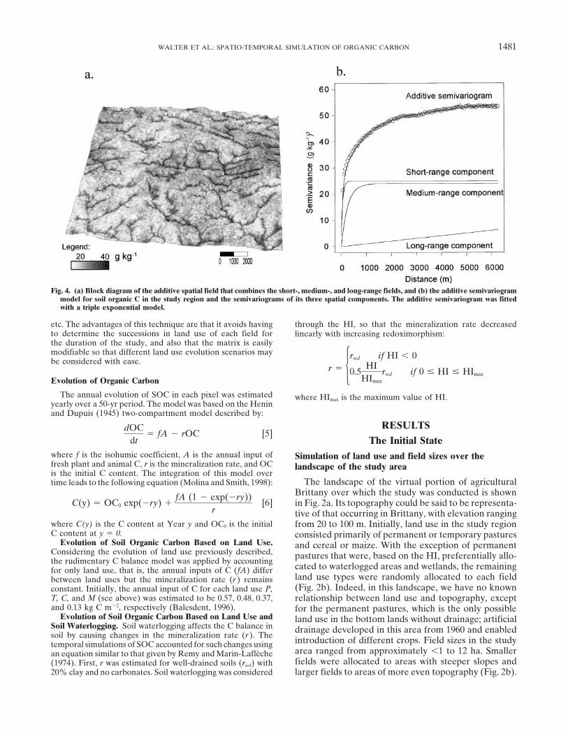
Fig. 4. (a) Block diagram of the additive spatial field that combines the short-, medium-, and long-range fields, and (b) the additive semivariogrammodel for soil organic C in the study region and the semivariograms of its three spatial components. The additive semivariogram was fittedwith a triple exponential model.

etc. The advantages of this technique are that it avoids having through the HI, so that the mineralization rate decreasedto determine the successions in land use of each field for linearly with increasing redoximorphism:the duration of the study, and also that the matrix is easilymodifiable so that different land use evolution scenarios maybe considered with ease.

r � �rwd if HI � 0

0.5HI

HImax

rwd if 0 � HI � HImaxEvolution of Organic Carbon

The annual evolution of SOC in each pixel was estimated where HImax is the maximum value of HI.yearly over a 50-yr period. The model was based on the Heninand Dupuis (1945) two-compartment model described by:

RESULTSdOCdt

� fA rOC [5]The Initial State

where f is the isohumic coefficient, A is the annual input of Simulation of land use and field sizes over thefresh plant and animal C, r is the mineralization rate, and OC landscape of the study areais the initial C content. The integration of this model over

The landscape of the virtual portion of agriculturaltime leads to the following equation (Molina and Smith, 1998):Brittany over which the study was conducted is shown

C(y) � OC0 exp(ry) �fA (1 exp(ry))

r[6] in Fig. 2a. Its topography could be said to be representa-

tive of that occurring in Brittany, with elevation rangingwhere C(y) is the C content at Year y and OC0 is the initial from 20 to 100 m. Initially, land use in the study regionC content at y � 0. consisted primarily of permanent or temporary pastures

Evolution of Soil Organic Carbon Based on Land Use. and cereal or maize. With the exception of permanentConsidering the evolution of land use previously described, pastures that were, based on the HI, preferentially allo-the rudimentary C balance model was applied by accounting

cated to waterlogged areas and wetlands, the remainingfor only land use, that is, the annual inputs of C (fA) differland use types were randomly allocated to each fieldbetween land uses but the mineralization rate (r) remains(Fig. 2b). Indeed, in this landscape, we have no knownconstant. Initially, the annual input of C for each land use P,

T, C, and M (see above) was estimated to be 0.57, 0.48, 0.37, relationship between land use and topography, exceptand 0.13 kg C m2, respectively (Balesdent, 1996). for the permanent pastures, which is the only possible

Evolution of Soil Organic Carbon Based on Land Use and land use in the bottom lands without drainage; artificialSoil Waterlogging. Soil waterlogging affects the C balance in drainage developed in this area from 1960 and enabledsoil by causing changes in the mineralization rate (r). The introduction of different crops. Field sizes in the studytemporal simulations of SOC accounted for such changes using

area ranged from approximately �1 to 12 ha. Smalleran equation similar to that given by Remy and Marin-Laflechefields were allocated to areas with steeper slopes and(1974). First, r was estimated for well-drained soils (rwd) with

20% clay and no carbonates. Soil waterlogging was considered larger fields to areas of more even topography (Fig. 2b).

1482 SOIL SCI. SOC. AM. J., VOL. 67, SEPTEMBER–OCTOBER 2003

Table 1. Transition probability matrix used to drive the land useevolution over time.

Permanent Temporarypastures pastures Cereals Maize

Permanent pastures 0.95 0.035 0.01 0.005Temporary pastures 0.01 0.65 0.24 0.1

Cereals 0.0 0.2 0.8 0.0Maize 0.0 0.09 0.01 0.90

Simulations of Soil Organic Carbon at DifferentSpatial Scales

The spatial variability of SOC in Brittany is assumedto occur at three different spatial scales: within fieldsdue to topography and agricultural management (short-range); between fields because of differences in land useor topographical position (medium-range); and betweenregions due to differences in climate and productionsystems (long-range). The semivariograms for the short-and long-range structures are shown in Fig. 3a and 3e,

Fig. 5. Simulations of land use over time driven by the transitionand realizations of their simulated RF models Y1(x) andmatrix given in Table 1, for maize (M), cereals (C), temporaryY2(x) are shown in Fig. 3b and 3f, respectively. Thepastures (T), and permanent pastures (P).medium-range spatial field was derived from a deter-

ministic relationship that equates the OC of the study additive spatial field has some important features: (i)area as a function of the soil HI derived from a DEM short-range variability between neighboring pixels; (ii)(Fig. 3c). The resulting medium-range spatial field Y3(x) higher values of OC in areas with high HI values, whichis shown in Fig. 3d. are generally riparian areas at the bottom of valleys;

(iii) a large trend of increasing SOC content from theCombination of the Random Functions south-west to north-east portions of the study area.Characterizing the Three Different Spatial Scales These features can also be recognized in the additive

experimental semivariogram (Fig. 4b), which shows aThe combined spatial field S(x) that characterizes therelatively high variance between pixels 50 m apart (thespatial variability of SOC at short-, medium-, and long-

range spatial scales is shown in Fig. 4a. The resulting first point on the experimental variogram), as part of

Fig. 6. Block diagrams of land use evolution at (a) the start of the simulation, (b) 10 yr after, (c) 20 yr after, and (d) at the end of the simulation:permanent pastures (P ), temporary pastures (T ), cereals (C ), and maize (M ).

WALTER ET AL.: SPATIO-TEMPORAL SIMULATION OF ORGANIC CARBON 1483

an initial steep increase in semivariance to a distance maize is 29.1%. Asymptotically, these final proportionsof 300 m, then a moderate increase to 2000 m and finally are independent of the initial state. Figure 5 shows thean asymptotic increase to distances greater than 6000 m. evolution of the proportions over time and indicates

that we have not reached the final proportions of theasymptote, but we are not far from it. The maps shownThe Dynamic (Temporal) Modelin Fig. 6 illustrate the evolution of land use over the

Temporal Land Use Evolution landscape at different dates after the start of the simu-lation.The transition matrix that was used to simulate the

temporal evolution of land use over time is given inEvolution of Soil Organic CarbonTable 1. The transition matrix produced a rapid evolu-

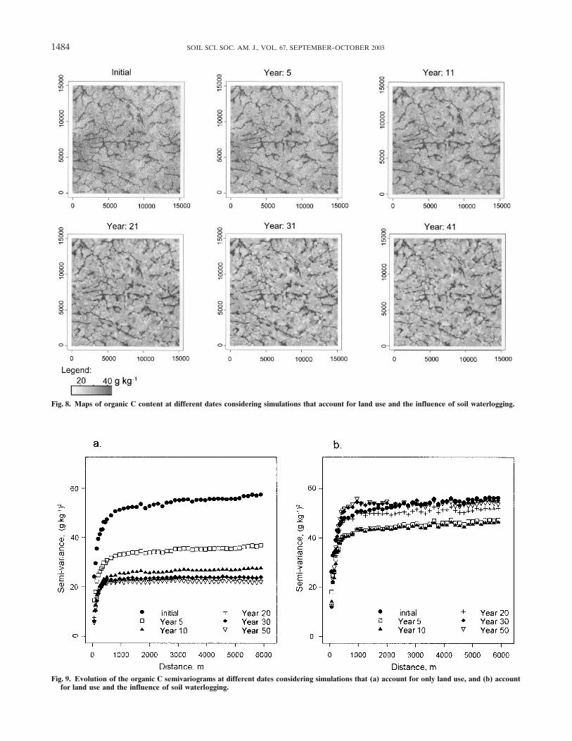
tion of land use over a relatively short period of time Simulated maps of SOC content produced under the(Fig. 5). Much like in Brittany, maize cropping increased assumption that land use is the only factor affecting itsrapidly while the area in permanent pastures decreased. evolution are shown in Fig. 7. The most apparent fea-The proportions of temporary pastures and cereals re- tures are the disappearance of the drainage pattern andmained constant throughout the simulation period long-range spatial trends, and the rapid development of(Fig. 5), however their allocation over the landscape medium range field patterns with an associated loss ofis assumed to have varied. The proportion of maize short-range variation within fields (Fig. 7).cropping in the study area increased from 5 to 25% Maps of SOC content simulated with the assumptionin 15 yr, while the proportion of permanent pastures that both land use and soil waterlogging affect its evolu-decreased from 30 to 10% in approximately 30 yr tion are shown in Fig. 8. In this instance, mineralization(Fig. 5). The final land use proportions are approached rates decreased with increasing HI value. The most ap-asymptotically: if Ly is the transition matrix, then Lp

y, as parent features of the simulations in Fig. 8 are the devel-p tends to infinity, has columns that are identical and opment of land use patterns and the disappearance ofrepresent the final proportions that each of the land long-range spatial trends. The network of redoximor-use types reaches. For our transition matrix (Table 1), phic areas associated with the medium-range structureasymptotically, the amount of permanent pastures is shows that higher amounts of SOC remained through-

out the simulation period (Fig. 8).5.7%, temporary pasture is 28.8%, cereal is 36.3%, and

Fig. 7. Maps of organic C content at different dates considering simulations that account only for land use.

1484 SOIL SCI. SOC. AM. J., VOL. 67, SEPTEMBER–OCTOBER 2003

Fig. 8. Maps of organic C content at different dates considering simulations that account for land use and the influence of soil waterlogging.

Fig. 9. Evolution of the organic C semivariograms at different dates considering simulations that (a) account for only land use, and (b) accountfor land use and the influence of soil waterlogging.

WALTER ET AL.: SPATIO-TEMPORAL SIMULATION OF ORGANIC CARBON 1485

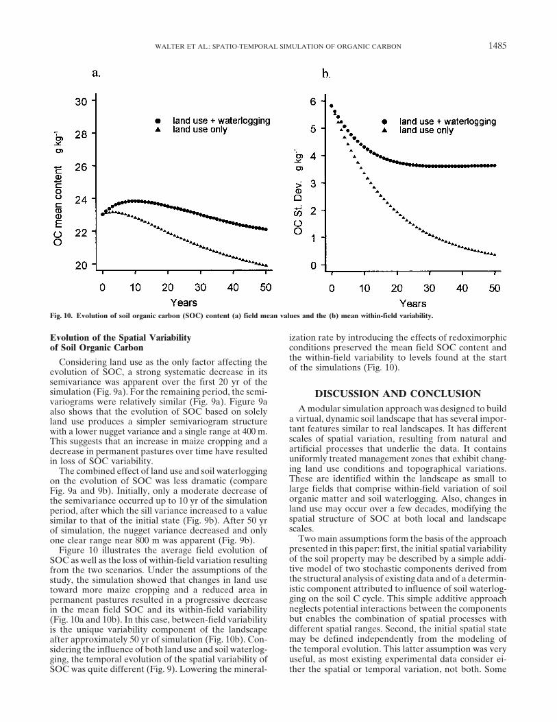
Fig. 10. Evolution of soil organic carbon (SOC) content (a) field mean values and the (b) mean within-field variability.

ization rate by introducing the effects of redoximorphicEvolution of the Spatial Variabilityconditions preserved the mean field SOC content andof Soil Organic Carbonthe within-field variability to levels found at the startConsidering land use as the only factor affecting theof the simulations (Fig. 10).evolution of SOC, a strong systematic decrease in its

semivariance was apparent over the first 20 yr of thesimulation (Fig. 9a). For the remaining period, the semi- DISCUSSION AND CONCLUSIONvariograms were relatively similar (Fig. 9a). Figure 9a

A modular simulation approach was designed to buildalso shows that the evolution of SOC based on solelya virtual, dynamic soil landscape that has several impor-land use produces a simpler semivariogram structuretant features similar to real landscapes. It has differentwith a lower nugget variance and a single range at 400 m.scales of spatial variation, resulting from natural andThis suggests that an increase in maize cropping and aartificial processes that underlie the data. It containsdecrease in permanent pastures over time have resulteduniformly treated management zones that exhibit chang-in loss of SOC variability.ing land use conditions and topographical variations.The combined effect of land use and soil waterloggingThese are identified within the landscape as small toon the evolution of SOC was less dramatic (comparelarge fields that comprise within-field variation of soilFig. 9a and 9b). Initially, only a moderate decrease oforganic matter and soil waterlogging. Also, changes inthe semivariance occurred up to 10 yr of the simulationland use may occur over a few decades, modifying theperiod, after which the sill variance increased to a valuespatial structure of SOC at both local and landscapesimilar to that of the initial state (Fig. 9b). After 50 yrscales.of simulation, the nugget variance decreased and only

Two main assumptions form the basis of the approachone clear range near 800 m was apparent (Fig. 9b).presented in this paper: first, the initial spatial variabilityFigure 10 illustrates the average field evolution ofof the soil property may be described by a simple addi-SOC as well as the loss of within-field variation resultingtive model of two stochastic components derived fromfrom the two scenarios. Under the assumptions of thethe structural analysis of existing data and of a determin-study, the simulation showed that changes in land useistic component attributed to influence of soil waterlog-toward more maize cropping and a reduced area inging on the soil C cycle. This simple additive approachpermanent pastures resulted in a progressive decreaseneglects potential interactions between the componentsin the mean field SOC and its within-field variabilitybut enables the combination of spatial processes with(Fig. 10a and 10b). In this case, between-field variabilitydifferent spatial ranges. Second, the initial spatial stateis the unique variability component of the landscapemay be defined independently from the modeling ofafter approximately 50 yr of simulation (Fig. 10b). Con-the temporal evolution. This latter assumption was verysidering the influence of both land use and soil waterlog-useful, as most existing experimental data consider ei-ging, the temporal evolution of the spatial variability of

SOC was quite different (Fig. 9). Lowering the mineral- ther the spatial or temporal variation, not both. Some

1486 SOIL SCI. SOC. AM. J., VOL. 67, SEPTEMBER–OCTOBER 2003

of stable carbon isotopes for estimating soil organic matter turnoverof the discrepancies that are apparent, particularly therates. Geoderma 82:43–58.fast decrease of the semivariance observed at the begin-

Chaplot, V., M. Bernoux, C. Walter, P. Curmi, and U. Herpin. 2001.ning of the simulation whatever the land use evolution Soil carbon storage prediction in temperate hydromorphic soilsscenario (Fig. 8), may nevertheless be attributed to the by using morphologic index and Digital Elevation Model. Soil

Sci. 166:48–60.simplified representation of the system.Chaplot, V., C. Walter, and P. Curmi. 2000. Improving soil hydromor-Modeling intends to capture the essentials of a system

phy prediction according to DEM resolution and available pedolog-and leave out what is considered secondary or relatively ical data. Geoderma 97:405–422.unimportant. In a regular modeling procedure, the accu- Collins, H.P., E.T. Elliot, K. Paustian, L.G. Bundy, W.A. Dick, D.R.

Huggins, A.J.M. Smucker, and E.A. Paul. 2000. Soil carbon poolsracy of the model should be validated by comparing itsand fluxes in the long-term corn belt agroecosystems. Soil Biol.predictions to experimental data. However, in this case,Biochem. 32:157–168.validation of the predicted temporal evolution of SOC Coppenet, M., J. Golven, J.C. Simon, L. Le Corre, and M. Le Roy.

content at the landscape scale is almost impossible as a 1993. Evolution chimique des sols en exploitation d’elevage inten-whole and only parts of the model may be compared sif: exemple du Finistere.(In French.) Agronomie (Paris) 13:77–83.

Cressie, N.A.C. 1991. Statistics for spatial data. John Wiley and Sons,with experimental data. Monitoring of different fieldsNew York.over time could be used to validate the apparent reduc-

Deutsch, C.V., and A.G. Journel. 1998. GSLIB, Geostatistical soft-tions in the spatial variability of SOC resulting from ware library and user’s guide. 2nd ed. Oxford University Press,different land use and uniform management. Also, com- New York.

Goovaerts, P. 1997. Geostatistics for natural resources evaluation.paring areas differing by the proportion of redoximor-Oxford Univ. Press, New York.phic soils could test the impact of soil waterlogging on

Goovaerts, P. 2000. Estimation or simulation of soil properties? An op-the SOC variability of the landscape. The procedures timisation problem with conflicting criteria. Geoderma 97:165–186.considered in this work attempt to simulate some fea- Hauhs, M. 1990. Ecosystem modelling: Science or technology? J. Hy-tures of the SOC balance in a region, while attempting drol. (Amsterdam) 116:25–33.

Henin, S., and M. Dupuis. 1945. Essai de bilan de la matiere organiqueto reproduce similar spatial structures and temporaldes sols.(In French.) Ann. Agron. 15:161–172.evolutions that occur in real landscapes.

Ibanez, J.J., S. De Alba, F.F. Bermudez, and A. Garcia Alvarez. 1995.A primary interest of simulating soil processes over Pedodiversity: Concepts and measures. Catena 24:215–232.time at the landscape scale is to assess soil management Jolivet, C., D. Arrouays, F. Andreux, and J. Leveque. 1997. Soil

organic carbon dynamics in cleared temperate forest spodosolspractices or sampling designs before their effective im-converted to maize cropping. Plant Soil. 191:225–231.plementation. Management practices may be evaluated

McBratney, A.B., B.M. Whelan, D.J.J. Walwoort, and B. Minasny.by their potential impact on both local and regional 1999. A purposive sampling scheme for precision agriculture.scales integrating evolutions over a few decades. For p. 101– 111. In J.V. Stafford. (ed.) Precision Agriculture’99. 2ndinstance, different strategies to increase C sequestration European Conference on Precision Agriculture, Odense Congress

Centre, Denmark.in soils may be tested including a comparison betweenMol, G., S.P. Vriend, and P.F.M. Van Gaans. 1998. Future trends, de-site specific (e.g., as permitted by precision agriculture)

tectable by soil monitoring networks? J. Geochem. Explor. 62:61–66.or uniform management. Another major interest of this Molina, J.A.E., and P. Smith. 1998. Modeling carbon and nitrogensimulation approach is to test sampling strategies for processes in soils. Adv. Agron. 62:253–298.

Nieder, R., and J. Richter. 2000. C and N accumulation in arabletheir ability to monitor the evolution of the landscapesoils of West Germany and its influence on the environment—components over time without bias and with minimalDevelopments 1970 to 1998. J. Plant Nutr. Soil Sci. 163:65–72.estimation errors. With our approach, such a predictive Oades, J.M. 1993. The role of biology in the formation, stabilisation

approach of the sensitivity of a planned sampling strat- and degradation of soil structure. Geoderma 56:377–400.Papritz, A., and R. Webster. 1995. Estimating temporal change in soilegy appears particularly useful as monitoring networks

monitoring. Eur. J. Soil Sci. 46:1–27.of soil quality are initiated in several countries (Mol etPhilip, J.R. 1991. Soils, natural science, and models. Soil Sci. 151:91–98.al., 1998). Different spatial configurations of the moni- Remy, J.C., and A. Marin-Lafleche. 1974. L’analyse de terre: Realisa-

toring networks can easily be implemented and the esti- tion d’un programme d’interpretation automatique.(In French.)Ann. Agron. 25:607–632.mated parameters compared with the “true” values of

Six, J., E.T. Elliott, and K. Paustian. 1999. Aggregate and Soil Organicthe virtual soil-landscape; the time interval between suc-Matter Dynamics under Conventional and No-Tillage Systems. Soilcessive sampling campaigns can also be optimized. Sci. Soc. Am. J. 63:1350–1358.

Smith, P., D.S. Powlson, M.J. Glendining, and J.O. Smith. 1997. Poten-tial for carbon sequestration in European soils: Preliminary esti-REFERENCESmates for five scenarios using results from long-term experiments.

Arrouays, D., W. Deslais, and V. Badeau. 2001. The carbon content Global Change Biol. 3:67–79.and its geographical distribution in France. Soil Use Manage. Stevenson, H.J. 1994. Humus chemistry. Genesis, composition, reac-17:7–11. tions. 2nd ed. John Wiley and Sons, New York.

Balabane, M., and J. Balesdent. 1995. Medium term transformations Walter, C. 1990. Soil properties estimation and quantification of theirof organic nitrogen in a cultivated soil. Eur. J. Soil Sci. 46:497–505. variability at medium scale. Ph.D diss. Univ. of Paris 6, Paris, France.

Baldock, J.A., and P.N. Nelson. 2000. Soil organic matter. p. B25–B84. Walter, C., C. Schvartz, B. Claudot, T. Bouedo, and P. Aurousseau.In M.E. Sumner (ed.) Handbook of Soil Science. CRC Press, Boca 1997. Statistical review of the soil tests made in France from 1990Raton, FL. to 1994: Statistical and cartographic descriptions of the cultivated

Balesdent, J. 1996. Un point sur l’evolution des reserves organiques topsoil horizon variability. Etude et Gestion des Sols 3:205–219.des sols en France. (In French.) Etude et Gestion des Sols 3:245–260. Wilson, J.P., and J.C. Gallant. 2000. Terrain analysis. Principles and

applications. John Wiley & sons, New York.Bernoux, M., C.C. Cerri, C. Neill, and J.F.L. Moraes. 1998. The use