Journal of Marine Systems 74 (2008) S86–S96

Contents lists available at ScienceDirect

Journal of Marine Systems

j ourna l homepage: www.e lsev ie r.com/ locate / jmarsys

Spatial predictions of Baltic phytobenthic communities: Measuringrobustness of generalized additive models based on transect data

Antonia Sandman a,⁎, Martin Isaeus b, Ulf Bergström c, Hans Kautsky a

a Department of Systems Ecology, Stockholm University, 106 91 Stockholm, Swedenb AquaBiota Water Research, Stockholm, Swedenc Institute of Coastal Research, Swedish Board of Fisheries, Öregrund, Sweden

a r t i c l e i n f o

⁎ Corresponding author. Tel.: +46 8 161103.E-mail address: antonia@ecology.su.se (A. Sandma

0924-7963/$ – see front matter © 2008 Elsevier B.V.doi:10.1016/j.jmarsys.2008.03.028

a b s t r a c t

Article history:Received 30 August 2007Received in revised form 28 December 2007Accepted 25 March 2008Available online 22 October 2008

The spatial distributions of benthic surface sediments and phytobenthic plant species weremodelled at a high spatial resolution using generalized additive models together with field datafrom diving transects. The efficiency of different modelling options was validated usingindependent datasets, and model fit versus predictive power was analysed. For rock/boulder,sand and mud/clay increasing complexity of the model resulted in higher Reciever OperatingCharacteristics (ROC) values for the model fit, but lower ROC values for the independentvalidation. The same patternwas found for hard substrate algae species, whereas it was not truefor the rooted plant species. As high model ROC values were often found to be connected to lowpredictive power of the models, this implies that internal model validation results should betreated cautiously. In general, the models should be kept simple, as the performance of theexplanation model increases with increasing complexity, while the predictive power of themodel generally decreases. Only by using external validation datasets, the true predictivecapacity of an explanation model can be reliably measured, as internal validation schemes tendto over-estimate model performance. Our results also indicate that the Akaike InformationCriterion is a more reliable model selection method than Cross-selection when there are fewpredictor variables.

© 2008 Elsevier B.V. All rights reserved.

Keywords:Spatial distributionGAMAICCross-selectionPhytobenthic speciesLine transects

1. Introduction

Accurate maps of underwater habitats are crucial for anefficient management of marine areas. As marine surveys areboth costlyand technically verydemanding, detailedknowledgeon thedistributionsofmarineorganisms ishowever very sparse.Within EU the need for concentrated efforts in marine habitatmapping has beenmade clear by effective directives such as theHabitats directive and theWater Framework directive.

Interestingly, recent advances in both survey techniquesand statistical handling of spatial data has opened up thepossibility to use predictive spatial modelling for producingreliable maps of the distributions of species and communities(Guisan and Thuiller 2005; Maggini et al., 2006). This gives anopportunity to translate data into broad scale areal coverage,

n).

All rights reserved.

which can be used to follow changes on both temporal andspatial scales, and to quantitatively evaluate the effects ofchanges in the ecosystem.

In this study, we performed high-resolution spatial model-ling of phytobenthic biota using data from linear divingtransects collected within the Swedish environmental mon-itoring programme. The statistical relationship betweenresponse and predictor variables was described using General-ized Additive Models (GAM). Much effort was allocated totesting the efficiency of differentmodelling options, as very fewstudies exist so far aiming at modelling marine phytobenthos.

The specific objectives of the study were to:

i) Test the use of linear transect data for modelling.ii) Test the effect of different selection methods and

different degrees of complexity of the model, com-pared to an external validation dataset.

iii) Investigate the general validity of the model.

S87A. Sandman et al. / Journal of Marine Systems 74 (2008) S86–S96

With increasing complexity of the model, the fit of thedata sets increases, whereas the predictive power of themodel outside the data may decrease, i.e. the model becomesoverfitted. Lehmann et al. (2002) recommend using fourdegrees of freedom of the spline smoothers in GAM model-ling, but we have not found a proper test that explains howdifferent degrees of freedom influence the model robustness.

Fig. 1. Map of the

We used an independent dataset for evaluation of modelpredictions to test how the model selection method andmodel complexity affected the predictive capacity of themodel. Specifically, we compared the performance of themodel selection methods AIC and Cross-selection, as well asthe performance of models based on different degrees offreedom of the GAM spline smoothers. These modelling

Askö area.

Table 1Response variables, a) substrate (including supplementary data), b) vegetation

Training data Validation data

Name Cover N Ntot Prevalence N Ntot Prevalence

a)Rock/boulder 25% 1866 3569 0.52 13 64 0.20Stone/gravel 25% 1381 3569 0.39 10 64 0.16Sand 25% 616 3569 0.17 18 64 0.28Mud/clay 25% 322 3569 0.09 33 64 0.52

b)Fucusvesiculosus

Presence 1069 3906 0.27 35 64 0.55

Fucusvesiculosus

25% 431 3906 0.11 7 64 0.11

Ceramiumtenuicorne

Presence 1771 3906 0.45 7 64 0.11

Furcellarialumbricalis

Presence 2084 3906 0.53 7 64 0.11

Potamogetonpectinatus

Presence 888 3906 0.23 40 64 0.63

Potamogetonpectinatus

25% 502 3906 0.13 19 64 0.30

Potamogetonprefoliatus

Presence 345 3906 0.09 23 64 0.36

Zosteramarina

Presence 429 3906 0.11 6 64 0.09

S88 A. Sandman et al. / Journal of Marine Systems 74 (2008) S86–S96

options were run on a set of habitats and species, consisting offour benthic substrate classes, three macroalgal species andthree vascular plants.

2. Methods

2.1. Study area

The Baltic Sea is one of the largest brackish water areas inthe world, with a salinity gradient from 20 psu in the Kattegatto 1–2 psu in the northernmost Bothnian Bay (c.f. Kautsky1995). The reduced salinity influences the biomass and speciescomposition (see for example Remane and Schlieper 1971;Kautsky 1995), and results in a species-poor flora and faunacompared to fully marine environments. The number ofmarine species decreases when passing the Danish straits,and continues to decrease northward into the Baltic Sea(Kautsky 1995; Snoeijs 1999), while the number of freshwaterspecies that can survive increases (Kautsky 1988; Kautsky andvan der Maarel 1990; Kautsky 1995). The geographic distribu-tion and the depth zonation of aquatic biota are set by bioticand abiotic factors, such as competition for space (Berger et al.,2001), grazing (Engkvist et al., 2000; Worm et al., 2001),salinity, depth, wave exposure and substrate. The abioticfactors can be used to predict the distribution of biota, whilethe biotic factors aremuchmore difficult to use in a large scalespatial context. Salinity is considered the most importantfactor governing the distribution at a large spatial scale in theBaltic Sea (c.f. Kautsky 1995), since it limits species of bothmarine and limnic origin. At a local scale, depth (i.e. lightavailability), wave exposure and substrate have been shown tobe the main factors shaping the distribution of phytobenthicspecies (Kautsky and van der Maarel 1990; Eriksson andBergström 2005).

The study area was the archipelago around the island ofAskö in the north west part of the Baltic proper (Fig. 1), wherethe salinity is fairly constant around 6.5 psu, with extremesbetween 5.5 psu and 8.0 psu (Larsson 2007). There is agradient from inner to outer archipelago in terms ofincreasing wave exposure (Isaeus 2004). There are practicallyno tides, and the upper limit to vegetation is set by low-waterperiods and ice-scouring (Kautsky and Kautsky 1989).

2.2. Data

The environmental monitoring datawere diving transects,sampled as line transects. Along an approximately 10 mwidecorridor, scuba divers followed a tape measure placed on thebottom surface, starting in the deep end and swimmingtowards the shore. The scuba divers continuously classifiedthe type of substrate and noted cover degree of plants in 7classes (1%, 5%, 10%, 25%, 50%, 75% and 100%), together withthe presence of animals. A new transect segment was startedwhenever there were major changes in the substrate orcommunity composition, or a new species appeared. Fordetailed description c.f. Jansson andKautsky (1977) or Kautsky(1995).

The line transects were subsampled into points every halfmeter, assigning the information in each segment of thetransect to all points within that segment (Table 1). For eachpoint, depth was calculated from the minimum and max-

imum depth of the transect segments, through linearinterpolation. The half meter distance was chosen to reflectthe spatial distribution of the transect segments within eachpixel in a proper way. The subsampling method may generateproblems with spatially autocorrelated data within thetransects, as the samples are closely located. However, usingonly one randomly selected observation from each transectwould be a tremendous loss of information. Therefore wewanted to analyse the effects on the modelling ability, whenviolating this statistical rule, by comparing to an externalvalidation dataset. We tested the impact of transect data inthe so called “substrate model”. Here we tried three differentapproaches with increasing amount of data used fromtransects, but also increasing interdependency. Finally, wevalidated the different methods using an independentdataset, to see if the validations improved with increasingamount of data.

There are a number of settings for GAMs, concerningstatistical selection methods and the complexity of theGAM functions which is set by the degrees of freedom forthe cubic spline smoothers that build up the model. Themost widely used model selection method for GAMs is theAkaike Information Criterion, AIC (recommended by e. g.Burnham and Anderson 2002), but recently anothermethod, Cross-selection, has been recommended byMaggini et al. (2006).

2.2.1. PredictorsAll predictor factors used in the models must be spatially

described as grids in order to create spatial models ingeographic information systems (GIS). In most Europeanwaters, including the study area, shallow seafloor substratesare not mapped at a spatial scale sufficient for accuratehabitat modelling. A comparison between observedsubstrate information in the datasets, and the reclassified

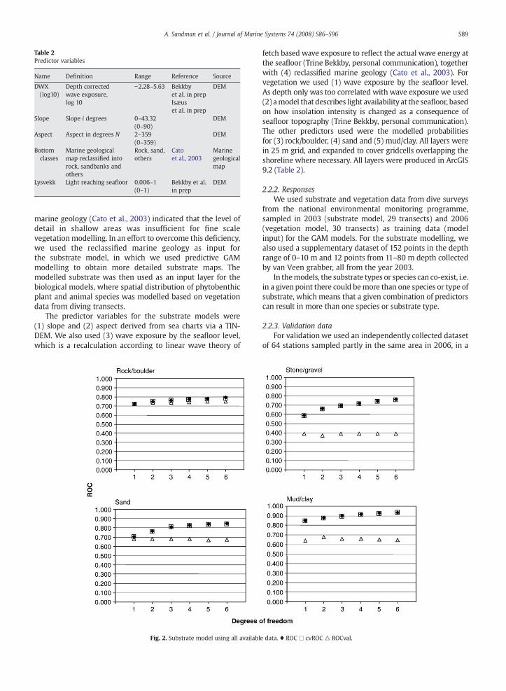
Table 2Predictor variables

Name Definition Range Reference Source

DWX(log10)

Depth correctedwave exposure,log 10

−2.28–5.63 Bekkbyet al. in prep

DEM

Isæuset al. in prep

Slope Slope i degrees 0–43.32 DEM(0–90)

Aspect Aspect in degrees N 2–359 DEM(0–359)

Bottomclasses

Marine geologicalmap reclassified intorock, sandbanks andothers

Rock, sand,others

Catoet al., 2003

Marinegeologicalmap

Lysvekk Light reaching seafloor 0.006–1 Bekkby et al.in prep

DEM(0–1)

S89A. Sandman et al. / Journal of Marine Systems 74 (2008) S86–S96

marine geology (Cato et al., 2003) indicated that the level ofdetail in shallow areas was insufficient for fine scalevegetation modelling. In an effort to overcome this deficiency,we used the reclassified marine geology as input forthe substrate model, in which we used predictive GAMmodelling to obtain more detailed substrate maps. Themodelled substrate was then used as an input layer for thebiological models, where spatial distribution of phytobenthicplant and animal species was modelled based on vegetationdata from diving transects.

The predictor variables for the substrate models were(1) slope and (2) aspect derived from sea charts via a TIN-DEM. We also used (3) wave exposure by the seafloor level,which is a recalculation according to linear wave theory of

Fig. 2. Substrate model using all availabl

fetch based wave exposure to reflect the actual wave energy atthe seafloor (Trine Bekkby, personal communication), togetherwith (4) reclassified marine geology (Cato et al., 2003). Forvegetation we used (1) wave exposure by the seafloor level.As depth only was too correlated with wave exposure we used(2) amodel that describes light availability at the seafloor, basedon how insolation intensity is changed as a consequence ofseafloor topography (Trine Bekkby, personal communication).The other predictors used were the modelled probabilitiesfor (3) rock/boulder, (4) sand and (5) mud/clay. All layers werein 25 m grid, and expanded to cover gridcells overlapping theshoreline where necessary. All layers were produced in ArcGIS9.2 (Table 2).

2.2.2. ResponsesWe used substrate and vegetation data from dive surveys

from the national environmental monitoring programme,sampled in 2003 (substrate model, 29 transects) and 2006(vegetation model, 30 transects) as training data (modelinput) for the GAM models. For the substrate modelling, wealso used a supplementary dataset of 152 points in the depthrange of 0–10 m and 12 points from 11–80 m depth collectedby van Veen grabber, all from the year 2003.

In themodels, the substrate types or species can co-exist, i.e.in a given point there could bemore than one species or type ofsubstrate, which means that a given combination of predictorscan result in more than one species or substrate type.

2.2.3. Validation dataFor validation we used an independently collected dataset

of 64 stations sampled partly in the same area in 2006, in a

e data. ♦ ROC □ cvROC △ ROCval.

Fig. 4. Substrate model using one point per transect segment. ♦ ROC □ cvROC △ ROCval.

Fig. 3. Substrate model using one point per transect plus supplementary data. ♦ ROC □ cvROC △ ROCval.

S90 A. Sandman et al. / Journal of Marine Systems 74 (2008) S86–S96

Fig. 5. Vegetation.

S91A. Sandman et al. / Journal of Marine Systems 74 (2008) S86–S96

depth range between 0 and 6 m. The cover of differentsubstrate types and species of vegetation was estimated in5 m radius circular areas by a snorkeller. The validation

stations were distributed within the same range of waveexposure, depth and insolation intensity as the trainingdataset.

Table 3Number of runs (of 48) where the selection methods tested gives the betterresult for ROC, cvROC and ROCval

ROC cvROC ROCval

AIC 26 21 32Cross-selection 22 25 16No difference 0 2 0

S92 A. Sandman et al. / Journal of Marine Systems 74 (2008) S86–S96

2.3. Models

GAMs were used to model the probability of occurrence ofsubstrates and species, using GRASP (Generalized RegressionAnalysis and Spatial Prediction) ver 3.3 (Lehmann et al., 2002)for S-plus (Insightful Corp., Seattle, WA, USA).

The different models were run with 1–6 degrees offreedom for the spline smoothers and Reciever OperatingCharacteristic curves, ROC, for both model and validationoutput were calculated according to Zweig and Campbell(1993). Cross validation ROC (cvROC) curves, which is aninternal validation of the model, were calculated by GRASP.The substrate models used to test the influence of datainterdependency were selected using Akaike InformationCriterion, AIC. For the vegetation model both AIC and Cross-selection were tested, as we wanted to test the influence ofselection method on the predictions. However, the substrateprobability layers used as indata in the vegetation modellingwere predicted using AIC and Cross-selection respectively.

2.3.1. Substrate modelIn the substrate modelling, we tested three different

approaches, utilising the diving transect dataset to differentdegrees. The datasets used: 1) all half-meter points (3405points), 2) a random selection of one point per belt (453 points),and 3) a random selection of one point per transect (29 points).In order to stabilise the model, we also chose to use thesupplementary dataset of 164 points collected by van Veengrabber for all three approaches.

For each point the substrate classes were aggregated intothe classes rock/boulder, stone/gravel, sand and mud/clay.Only substrate records covering N=25% of the seafloor weretaken into account, and converted into presence/absence.

2.3.2. Vegetation modelIn the vegetation models we used presence of six different

species, Fucus vesiculosus, Furcellaria lumbricalis, Ceramiumtenuicorne, Potamogeton pectinatus, Potamogeton perfoliatusand Zostera marina. The first three species are found on hardsubstrates, whereas the latter are rooted plants and thusmainly found on gravel and finer sediments. For F. vesiculosusand P. pectinatus we also modelled occurrences of 25%coverage or more, from hereon referred to as meadows.Those two species were the only ones with frequentoccurrences of 25% coverage or more in the validation dataset(present in 35 and 40 points respectively and present as 25%coverage or more in 7 and 19 points).

2.4. Spatial predictions

In order to make spatial predictions of occurrence of themodelled species, the models were exported to ArcView 3.3(ESRI) from S-plus as lookup-tables (Lehmann et al., 2002).

3. Results

3.1. Substrate model

For the rock/boulder, sand and mud/clay, increasingdegrees of freedom for the spline functions gave highermodel ROC (Reciever Operating Curves) but lower validation

ROC. For stone/gravel substrates the validation resulted inROCb0.5 for all degrees of freedom (Fig. 2), so the predictionsof stone/gravel were excluded from further modelling. In thetest of transect model, the performance as well as thevalidation was poor when using only one point per transectcompared to using all points (Figs. 2 and 3). Using one pointper transect segment (i.e. the different parts of the lineartransect that the diver had classified as separate units) did notresult in the same loss (Fig. 4).

3.2. Vegetation model AIC

For the predicted presence/absence of F. vesiculosus, themodel ROC increased from 0.76 to 0.86with increasing degreesof freedom from1 to6,while the validationROCdecreased from0.66 to 0.59 (Fig. 5). For theprediction ofF. vesiculosusmeadows,with occurrence of 25% coverage or more, the model ROCincreased from 0.85 to 0.92 with increasing df, while thevalidation ROC decreased from 0.54 to 0.48, which means thatmodelling ofmeadows rather thanpresence/absence is difficultfor F. vesiculosus.

The same pattern was found for the predicted presence/absence of C. tenuicorne, where themodel ROC increased from0.73 to 0.86, while validation ROC decreased from 0.75 to 0.71(although it increased to 0.77 at 2 degrees of freedom), and forF. lumbricalis where the model ROC increased from 0.75 to0.84, validation ROC decreased from 0.84 to 0.75 (Fig. 5).

In the P. pectinatus presence/absence model, the modelROC increased from 0.82 to 0.91, and the validation ROCincreased from 0.49 to 0.61. For the prediction of P. pectinatusmeadows, the model ROC increased from 0.88 to 0.97, whilethe validation ROC ranges between 0.49 (2 df) and 0.55 (6 df)(no trend). The modelling of P. pectinatus meadows is thus asdifficult as for F. vesiculosus. For the presence/absence of P.perfoliatus themodel ROC increased from 0.86 to 0.95, and thevalidation ROC ranged between 0.55 (3 df) and 0.62 (1 df) (notrend) and for Z. marina themodel ROC increased from 0.92 to0.98, while the validation ROC increased from 0.57 to 0.66(weak trend) (Fig. 5).

3.3. Vegetation model Cross-selection

For F. vesiculosuspresence/absence themodel ROC increasedfrom 0.75 to 0.86 with increasing df (2–6), while the validationROC decreased from0.69 to 0.50. For F. vesiculosusmeadows themodel ROC increased from0.84 to 0.93with increasingdf, whilethe validation ROC decreased from 0.55 to 0.44. The samepatternwas found for presence/absence of F. lumbricalis (modelROC increased from0.74 to 0.85, validation ROC decreased from0.84 to 0.71. For presence/absence of C. tenuicorne the model

Fig. 6. Predictions of vegetation. Probability of presence of a. Fucus vesiculosus, b. Ceramium tenuicorne, c. Furcellaria lumbricalis, d. Potamogeton pectinatus,e. Potamogeton perfoliatus, f. Zostera marina at 0–20 m depth.

S93A. Sandman et al. / Journal of Marine Systems 74 (2008) S86–S96

S94 A. Sandman et al. / Journal of Marine Systems 74 (2008) S86–S96

ROC increased from 0.75 to 0.85, while the validation ROChovers between 0.64 (4 df) and 0.71 (3 df) (Fig. 5).

In the P. pectinatus presence/absence model, the modelROC increased from 0.80 to 0.91, and the validation ROCincreases from 0.51 to 0.69. For P. pectinatus meadows, themodel ROC increases from 0.89 to 0.97, while the validationROC ranges between 0.45 (1 df) and 0.54 (5 df). For presence/absence of P. perfoliatus the model ROC increased from 0.86 to0.94, and the validation ROC ranges between 0.62 (1 df) and0.52 (3 df) and for presence/absence of Z. marina the modelROC increased from 0.93 to 0.98, and the validation ROCranges between 0.46 (1 df) to 0.67 (4 df) (Fig. 5).

The maximum differences in ROC values between AIC andCross-selection were 0.02 for ROC and cvROC, and 0.17 forvalidation ROC. In two thirds of the model runs the validationROC for AIC is higher than for Cross-selection (Table 3). Themodel ROC and the cross-validation ROC differ very little,independent of selection method.

4. Predictions

The predictions were made using two degrees of freedomfor the spline smoothers. The substrate model gives highprobabilities of rock/boulder at exposed sites, and mud/clay atsheltered sites, whereas sand is predicted to have a patchydistribution. For the vegetation model, F. vesiculosus waspredicted to occur at moderately to highly exposed sites,whileC. tenuicorne and F. lumbricaliswere predicted to be foundon sites with high exposure levels, with F. lumbricalis in deeperareas. P. pectinatus and P. perfoliatuswere predicted to be foundat sheltered sites, although P. pectinatus would be the morecommon. Z. marina was predicted to occur at moderately tohighly exposed sites (Fig. 6).

5. Discussion

5.1. Model data

The data used for modelling mainly came from divingtransects shallower than 10m depth, but also included deeperdiving observations and for the substratemodel data fromvanVeen grabs were used as well. The external validation datasetwas collected with a different method and with a differentfocus. According to Elith et al. (2006) an independentlycollected dataset is important in order to have a truevalidation of the model. The environmental limits (depthrange, wave exposure values etc) in the validation datasetwere completely covered by those of the training data. Thetrends for the Furcellaria, Ceramium and Fucus models weresimilar,with increasing gap betweenmodel and validation forincreasing degrees of freedom, which supports the idea thatsimplemodels are preferred to more complex ones, as the riskof overfitting the model is lower (c.f. Burnham and Anderson2002). In the substrate model, the stones/gravel substrateswere present in 10 points in the validation dataset, whilerock/boulder substrates were present in 13 points, sand in 18and mud/clay in 33 points. The stones/gravel substrate wasalso the one with the lowest ROC values in the validation,although this might be a general modelling problem; it iseasier to model hard substrates and fine sediments, whereasthe intermediate classes are more dependent on the given

quaternary geological processes and history, and less onenvironmental conditions, and thus less predictable.

For some species, the limited size of the validation dataset,with 64 independent points, might have influenced theevaluation results. For example, in F. lumbricalis and C.tenuicorne the validation ROC was higher than the model ROCfor somedegrees of freedom. Thismight be due to lowpresenceof these species in the validation dataset (in 7 points out of 64for both species). The general conclusion that simple modelsproduce better predictions than complex ones is, however, notaffected by these inconsistencies.

5.2. Transect data

In the test of how transect resampling intensity affects thepredictive power, we also used a supplementary dataset fromvan Veen grabs, to stabilise the model as randomisation attransect level gave too few points (29) to build a model. Usingonly one point per transect segment produced too few pointsfor the model to make any predictions, and it seemedunreasonable to be that strict in treating data. By using allpoints from the transect data, information on the spatialdistribution and width of the transect segment was utilised,not just the position, this adding a quantitativemeasure of theabundance of the species. Using one random point persegment produced similar, but less accurate, predictionscompared to the models utilising all point data. This loss ofaccuracy is likely due to a loss of information on prevalenceand spatial representation of the species.

5.3. Degrees of freedom of spline smoothers

Generally, increasing degrees of freedom for the splinesmoothers resulted in higher ROC and cvROC, but equal orlower validation ROC. This indicates that the model getsoverfitted with increasing degrees of freedom. If we look onlyat the internal validation, this pattern is however not visible,suggesting that internal cross-validation is not sufficient todetermine the proper degrees of freedom. A restrictiveapproach of one to three degrees of freedom in generalproduced the highest ROC values in the external validation,suggesting that the recommendation of four degrees offreedom provided by Lehmann et al. (2002) may sometimesproduce overfitted models. However, one degree of freedomin GRASP gives a linear response, why the benefits of usingGAM over linear regression is lost (Austin 2007). We thereforerecommend the use of two to three degrees of freedom.

5.4. AIC vs. Cross-selection

According to Maggini et al. (2006) the Cross-selectionoption in GRASP gives better predictions than AIC, based onthe cvROC, as AIC is considered too liberal (Kuha 2004;Maggini et al., 2006). Our results indicate that the differencebetween the two selection methods can be ignored whenlooking only at cvROC, as the difference between predictionand validation still outranges the differences in method orbetween ROC and cvROC. When we look at the externalvalidation however, it is evident that the models selected byAIC are stronger than those selected by Cross-selection.This result is probably valid for models with few predictor

S95A. Sandman et al. / Journal of Marine Systems 74 (2008) S86–S96

variables, as the risk of adding too many variables with AICbecomes quite small.

5.5. General validity

The algal models were, according to the external valida-tion, more accurate than the rooted plant models. As therooted plants are found on sediments up to the size of gravel,the poor outcome of the stones/gravel model might nega-tively influence the result. Although we evaluated the gravel/stones model and found it too weak to be included in themodel, the information is missing, although it might still beneeded to make good predictions of rooted plants. A lowprevalencemay also reduce the explanatory power of a model(Austin and Meyers 1996), which may have affected therooted plant model. However, as the prevalence of the speciesin this study ranged between 0.09 and 0.53, this effect shouldbe negligible (Maggini et al., 2006). Also, information outsidethe environmental range of the species is important from amodelling perspective as the true response curve can only bedetermined if the sampling exceeds the environmentalgradient of the species (Austin 2007). Thus zeroes wherethe species could not be present would rather strengthen themodel.

The use of transect data results in interdependent data. Asthe internal validation (cvROC) is based on a selection of thetotal prediction dataset, the cvROC will be close to the modelperformance ROC. The results demonstrate the difficulty toassess the true validity of the cvROC, so the internal validationcannot be trusted as an alternative to an independent dataset.

6. Conclusions

In this study we evaluated the use of data from lineartransects for GAM modelling, as linear transects is acommonly used survey method. Using all the points fromthe transect data generated the best performing models,indicating that the potential negative effects of autocorrela-tion between data points is negligible compared to thebenefits of utilising all the information contained in thedatasets. The major drawback of using autocorrelated data inthis respect is that standard errors of model parameters willbe biased; giving rise to too liberal statistical significance tests(Zhang et al., 2005). The model results may still be veryinformative regarding the relationships between predictorand response variables. Thus, a high resampling intensity oftransect data may be recommended, at least at someinstances, when the goal is producing accurate predictionsrather than developing ecological theory.

The model selection methods AIC and Cross-selectiondiffer in their merits. Cross-selection has previously beenrecommended as a selection method in GAM modelling(Maggini et al., 2006), while in this study AIC proved to be amore efficient selection method. Our results indicate that AICis a more reliable model selection method than Cross-selection when the set of predictor variables to build themodel on is small, and the risk of adding too many variableswith AIC is limited, although it generally considered toopermissive (Kuha 2004; Maggini et al., 2006).

We have also evaluated the use of degrees of freedomfor the spline smoothers in GAM, in order to construct

robust models for species distribution. The ROC-valueproduced by the model is not necessary a measure ofmodel performance. On the contrary, very high model ROC-values were often found to be connected to low validationvalues. We thus recommend that the degrees of freedom ofthe GAM spline smoothers should be kept low, as theperformance of the explanation model increases withincreasing degrees of freedom, while the predictive powerof the model generally decreases. Thus, cvROC may often bean unreliable measure of the predictive power of a model.Only by using external validation datasets, the truepredictive capacity of an explanation model can be reliablymeasured.

Acknowledgements

Supplementary substrate data was kindly provided byHans Cederwall.

References

Austin, M.P., 2007. Species distribution models and ecological theory: acritical assessment and some possible new approaches. EcologicalModelling 200 (1–2), 1–19.

Austin, M.P., Meyers, J.A., 1996. Current approaches to modelling theenvironmental niche of eucalypts: implication for management of forestbiodiversity. Forest Ecology and Management 85 (1–3), 95–106.

Berger, R., Malm, T., Kautsky, L., 2001. Two reproductive strategies in BalticFucus vesiculosus (Phaeophyceae). European Journal of Phycology 36(3), 265–273.

Burnham,K.P., Anderson,D.R., 2002.Model Selection andMultimodel Inference.A Practical Information-Theoretic Approach, 2nd ed. Springer-Verlag,New York, p. 488.

Cato, I., Kjellin, B., Zetterlund, S., 2003. Förekomst och utbredning avsandbankar, berg och hårdbottnar inom svenskt territorialvatten ochsvensk ekonomisk zon (EEZ). SGU Rapport 2003:1. Sveriges GeologiskaUndersökning (SGU), Uppsala.

Elith, J., Graham, C.H., Anderson, R.P., Dudík, M., Ferrier, S., Guisan, A.,Hijmans, R.J., Huettmann, F., Leathwick, J.R., Lehmann, A., Li, J., Lohmann,L.G., Loiselle, B.A., Manion, G., Moritz, C., Nakamura, M., Nakazawa, Y.,Overton, J. McC., Peterson, A.T., Phillips, S.J., Richardson, K.S., Scachetti-Pereira, R., Schapire, R.E., Sobero'n, J., Williams, S., Wisz, M.S.,Zimmermann, N.E., 2006. Novel methods improve prediction of species'distributions from occurrence data. Ecography 29 (2), 129–151.

Engkvist, R., Malm, T., Tobiasson, S., 2000. Density dependent grazing effectsof the isopod Idotea baltica Pallas on Fucus vesiculosus L in the Baltic Sea.Aquatic Ecology 34 (3), 253–260.

Eriksson, B.K., Bergström, L., 2005. Local distribution patterns of macroalgaein relation to environmental variables in the northern Baltic Proper.Estuarine, Coastal and Shelf Science 62, 109–117.

Guisan, A., Thuiller, W., 2005. Predicting species distribution: offering morethan simple habitat models. Ecology Letters 8 (9), 993–1009.

Isaeus, M., 2004. Factors structuring Fucus communities at open and complexcoastlines in the Baltic Sea. Doctoral dissertation, Department of Botany,Stockholm University, Stockholm, Sweden.

Jansson, A.-M., Kautsky, N., 1977. Quantitative survey of hard bottomcommunities in a Baltic archipelago. In: Keegan, B.F., Boaden, P.J.S.(Eds.), Biology of Benthic Organisms. Pergamon, New York, pp. 359–366.

Kautsky, L., 1988. Life strategies of aquatic soft bottommacrophytes. Oikos 53(1), 126–135.

Kautsky, H., 1995. Quantitative distribution of sublittoral plant and animalcommunities along the Baltic Sea gradient. In: Eleftheriou, A., Ansell, A.D.,Smith, C.J. (Eds.), Biology and Ecology of Shallow Coastal Waters (Proc.28th Europ. Mar. Biol. Symp., Crete). Olsen & Olsen, Fredensborg, Denmark,pp. 23–30.

Kautsky, L., Kautsky, H., 1989. Algal species diversity and dominance alonggradients of stress and disturbance in marine environments. Vegetatio83, 259–267.

Kautsky, H., van der Maarel, E., 1990. Multivariate approaches to the variationin phytobenthic communities and environmental vectors in the BalticSea. Marine Ecology Progress Series 60, 169–184.

Kuha, J., 2004. AIC and BIC. Comparisons of assumptions and performance.Sociological Methods & Research 33 (2), 188–229.

S96 A. Sandman et al. / Journal of Marine Systems 74 (2008) S86–S96

Larsson, U., 2007. Himmerfjärden eutrophication study. WWW Page, http://www2.ecology.su.se/dbhfj/index.htm.

Lehmann, A., Overton, J.McC., Leathwick, J.R., 2002. GRASP: generalizedregression analysis and spatial predictions. Ecological Modelling 157 (1–2),189–207.

Maggini, R., Lehmann, A., Zimmermann, N., Guisan, A., 2006. Improvinggeneralized regression analysis for the spatial prediction of forestcommunities. Journal of Biogeography 33 (10), 1729–1749.

Remane, A., Schlieper, C., 1971. Biology of Brackish Water. John Wiley & SonsInc, New York, p. 372.

Snoeijs, P., 1999. Marine and brackish waters. In: Rydin, H., Snoeijs, P.,Diekmann, M. (Eds.), Swedish Plant Geography: Dedicated to Eddy van

der Maarel on his 65th birthday. Acta Phytogeographica Suecica, 94,pp. 1–248.

Worm, B., Lotze, H.K., Sommer, U., 2001. Algal propagule banks modifycompetition, consumer and resource control on Baltic rocky shores.Oecologia 128 (2), 281–293.

Zhang, L., Gove, J.H., Heath, L.S., 2005. Spatial residual analysis of sixmodeling techniques. Ecological Modelling 186 (2), 154–177.

Zweig, M.H., Campbell, G., 1993. Receiver-Operating Characteristic (ROC)plots: a fundamental evaluation tool in clinical medicine. ClinicalChemistry 39 (4), 561–577.