ARTICLE IN PRESS

Contents lists available at ScienceDirect

Computers & Geosciences

Computers & Geosciences 35 (2009) 626–634

0098-30

doi:10.1

� Cor

E-m

journal homepage: www.elsevier.com/locate/cageo

Spatial data analysis of finite strain data across a thrust sheet using R

N. Iranpanah a, M. Mohammadzadeh a,�, M.Q. Vahidi Asl b, A. Yassaghi c

a Department of Statistics, Tarbiat Modares University, P.O. Box 14115-175 Tehran, Iranb Department of Statistics, Shahid Beheshty University, Evin, Tehran, Iranc Department of Geology, Tarbiat Modares University, P.O. Box 14115-175 Tehran, Iran

a r t i c l e i n f o

Article history:

Received 30 September 2007

Received in revised form

7 May 2008

Accepted 26 October 2008

Keywords:

Finite strain data

Nugget effect

Ordinary kriging

Robust kriging

04/$ - see front matter & 2008 Elsevier Ltd. A

016/j.cageo.2008.10.001

responding author. Tel./fax: +98 2182883483.

ail address: mohsen_m@modares.ac.ir (M. Mo

a b s t r a c t

In this paper, the finite strain data (FSD) collected from a Sheeprock thrust sheet in Utah

are spatially analyzed. The steps and special manner of spatial analysis of these data are

examined due to the importance and influence of data characteristics on spatial

prediction accuracy. To do so, the exponential and spherical parametric variogram

models with and without nugget effects are fitted by maximum likelihood and

restricted maximum likelihood methods on original and normally transformed data. We

also fitted other models to classical and robust empirical variograms by ordinary least

squares and weighted least squares methods. Next, these models are applied on data

and edited data by using robust kriging. Finally, the accuracy of the obtained results are

compared with Mukul’s model by cross-validation in order to choose the best variogram

model for FSD and also specify the importance of attention to characteristics of the data

in spatial data analysis.

& 2008 Elsevier Ltd. All rights reserved.

1. Introduction

Finite strain data (FSD) are an important part of thedata set in studying the geometry and kinematics of thrustsheets (Boyer, 1995; Mitra, 1997) and in the constructionof retrodeformable balanced geological cross-sections(Woodward et al., 1986; Mitra, 1994). In most orogenicbelts, thrust systems exhibit complex strain patterns andthe complexity of finite strain even increases fromexternal to internal thrust sheets (Mitra, 1994). Variationof finite strain can be shown by selecting samples fromeach thrust sheet as representative samples and quantify-ing their mean strain. However, this approach can neitheraccount for spatial variability of the data set nor be usedto predict strain values from the unsampled locations atany point within the sheet (Mukul, 1998). By implicationof a spatial statistical approach, not only the spatialvariability of FSD within and across thrust sheets can be

ll rights reserved.

hammadzadeh).

quantified but also the prediction on the finite strainvalues anywhere in the sample area can be made.

Spatial models (Cressie, 1993) have been extensivelyused in many disciplines, such as structural geology, thatemploy dependent data collected spatially from differentlocations. In spatial statistics, usually a random field isconsidered for modeling the data and the correlationstructure of the data is determined by a variogram.Accuracy of spatial data analysis severely depends onproperties of the random field such as being Gaussian,stationarity and isotropicity. This is certainly influencedby the existence of outlier observations. It also depends onhow well a variogram model is fitted. Therefore, a study ofthe data properties and fitting the best variogram modelare initial basic steps in exploratory analysis of the spatialdata.

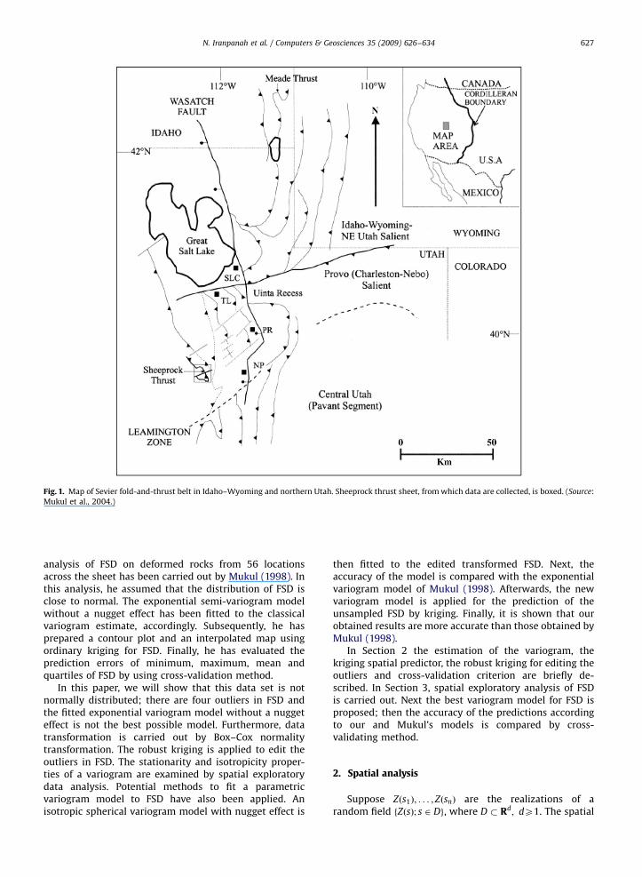
Foreland fold-thrust belts are the outer parts oforogenic belts in which rock deformation is spatiallyconcentrated across thrust sheets (Mitra, 1994). The Sevierfold-and-thrust belt in western United States consists ofseveral thrust sheets, one of which is the Sheeprock thrustsheet located in Provo salient of the belt (Fig. 1). Spatial

ARTICLE IN PRESS

Fig. 1. Map of Sevier fold-and-thrust belt in Idaho–Wyoming and northern Utah. Sheeprock thrust sheet, from which data are collected, is boxed. (Source:

Mukul et al., 2004.)

N. Iranpanah et al. / Computers & Geosciences 35 (2009) 626–634 627

analysis of FSD on deformed rocks from 56 locationsacross the sheet has been carried out by Mukul (1998). Inthis analysis, he assumed that the distribution of FSD isclose to normal. The exponential semi-variogram modelwithout a nugget effect has been fitted to the classicalvariogram estimate, accordingly. Subsequently, he hasprepared a contour plot and an interpolated map usingordinary kriging for FSD. Finally, he has evaluated theprediction errors of minimum, maximum, mean andquartiles of FSD by using cross-validation method.

In this paper, we will show that this data set is notnormally distributed; there are four outliers in FSD andthe fitted exponential variogram model without a nuggeteffect is not the best possible model. Furthermore, datatransformation is carried out by Box–Cox normalitytransformation. The robust kriging is applied to edit theoutliers in FSD. The stationarity and isotropicity proper-ties of a variogram are examined by spatial exploratorydata analysis. Potential methods to fit a parametricvariogram model to FSD have also been applied. Anisotropic spherical variogram model with nugget effect is

then fitted to the edited transformed FSD. Next, theaccuracy of the model is compared with the exponentialvariogram model of Mukul (1998). Afterwards, the newvariogram model is applied for the prediction of theunsampled FSD by kriging. Finally, it is shown that ourobtained results are more accurate than those obtained byMukul (1998).

In Section 2 the estimation of the variogram, thekriging spatial predictor, the robust kriging for editing theoutliers and cross-validation criterion are briefly de-scribed. In Section 3, spatial exploratory analysis of FSDis carried out. Next the best variogram model for FSD isproposed; then the accuracy of the predictions accordingto our and Mukul’s models is compared by cross-validating method.

2. Spatial analysis

Suppose Zðs1Þ; . . . ; ZðsnÞ are the realizations of arandom field fZðsÞ; s 2 Dg, where D � Rd; dX1. The spatial

ARTICLE IN PRESS

N. Iranpanah et al. / Computers & Geosciences 35 (2009) 626–634628

correlation structure of the random field is determined bythe variogram 2gðs1; s2Þ ¼ VarðZðs1Þ � Zðs2ÞÞ for alls1; s2 2 D. Under the intrinsic stationarity assumption, anunbiased estimator of the variogram is defined by

2gðhÞ ¼ 1

Nh

XNðhÞ

½ZðsÞ � Zðsþ hÞ�2, (1)

where NðhÞ ¼ fðsi; sjÞ : si � sj ¼ h; i; j ¼ 1; . . . ;ng and Nh isthe number of elements of NðhÞ. Cressie and Hawkins(1980) proposed the robust estimator of the variogramgiven by

2gðhÞ ¼

1

Nh

PNðhÞ jZðsiÞ � ZðsjÞj

1=2

� �4

0:475þ0:494

Nh

� � . (2)

Since the variogram estimators (1) and (2) cannot beused directly for spatial predictions, we need to fit a validvariogram model that is closest to the spatial dependencestructure present in the data. Various parametric vario-gram models are presented in Journel and Huijbregts(1978). Let P ¼ f2gð�; yÞ; y 2 Yg denote a parametricsubset of valid variograms. Several methods such asmaximum likelihood (ML), restricted maximum likelihood(REML), ordinary least squares (OLS) and weighted leastsquares (WLS) can be applied to estimate y (Cressie, 1993).

Considering the observations Z ¼ ððZðs1Þ; . . . ; ZðsnÞÞ, theordinary kriging refers to spatial prediction of the randomfield at a location s0 under the assumption that mðsÞ ¼ E½ZðsÞ�

is a fixed unknown real value m, and the predictor is anunbiased linear function of observations, i.e. Zðs0Þ ¼ l0Z withcoefficients l0 ¼ ðg� 1mÞ0G�1, where m ¼ �ð1� 10G�1gÞ=ð10G�11Þ, 1 ¼ ð1; . . . ;1Þ0; g ¼ ðgðs0 � s1Þ; . . . ; gðs0 � snÞÞ

0 andG is the n� n matrix whose ði; jÞth element is gðsi � sjÞ.

Table 1Base data values from Sheeprock thrust sheet.

i x y z i x y

1 810 3470 1.245 20 1355 3

2 975 3640 1.180 21 1505 3

3 1150 3830 1.325 22 1715 3

4 1880 4600 1.302 23 1865 3

5 2185 4850 1.233 24 2030 4

6 125 2340 1.305 25 2205

7 290 2530 1.301 26 2370 4

8 495 2715 1.339 27 550 2

9 665 2920 1.375 28 865 2

10 1000 3295 1.225 29 1040 2

11 1160 3495 1.222 30 1700 3

12 1325 3655 1.163 31 2040 3

13 1495 3855 1.067 32 2225 3

14 2200 4560 1.285 33 2405 4

15 2395 4760 1.127 34 2560

16 335 2170 1.319 35 725

17 525 2370 1.220 36 885 2

18 695 2545 1.276 37 1220 2

19 865 2745 1.260 38 2035 3

x (m) and y (m) are geographic coordinate location of analyzed sample. z is st

2004).

The minimized mean-squared prediction error, namely thekriging variance, is given by s2

k ðs0Þ ¼ l0gþm.The effect of outliers on inference procedures can be

substantial. Deleting outliers when estimating a variogrammay be sensible, but for the prediction, an alternative wayof dealing with them is needed. Hawkins and Cressie(1984) proposed a way of using neighboring values todetermine how much the outlier should be downweighted.In their method, namely robust kriging, the fitted vario-gram to the robust variogram (2) is used to compute thekriging weights to predict each ZðsjÞ by using all the dataexcept ZðsjÞ as

Z�jðsjÞ ¼Xn

ðiajÞ¼1

ljiZðsjÞ. (3)

Next, the weights in (3) are used to obtain a robustprediction of ZðsjÞ from its neighbors by

Z@�jðsjÞ ¼WMðfZðsiÞ : iajg; flji : iajgÞ,

where ‘‘WM’’ denotes the weighted median definedin Cressie (1993). Finally, ZðsjÞ is edited by replacingit with

ZðeÞðsjÞ ¼

Z@�jðsjÞ þ cs�jðsjÞ; Dj4dj;

ZðsjÞ; jDjjpdj;

Z@�jðsjÞ � cs�jðsjÞ; Djodj;

8>><>>: (4)

where Dj ¼ ZðsjÞ � Z@�jðsjÞ, dj ¼ cs�jðsjÞ, s2

�jðsjÞ is the asso-ciated kriging variance of Z�jðsjÞ and the positive constant c

controls the amount of editing applied to the outlyingvalues.

Assume that a predictor Zðs0Þ is available along with ameasure of its mean-squared prediction error s2

k ðs0Þ.Let 2gðh; yÞ be the fitted variogram model; now delete

z i x y z

300 1.226 39 925 1665 1.308

495 1.351 40 2065 2970 1.284

670 1.127 41 2420 3345 1.372

855 1.230 42 1115 1490 1.482

055 1.270 43 1265 1700 1.296

4210 1.400 44 1440 1890 1.308

375 1.318 45 1775 2275 1.352

005 1.250 46 2410 2980 1.207

395 1.196 47 1465 1525 1.301

600 1.357 48 1625 1740 1.299

325 1.243 49 2785 3010 1.316

695 1.149 50 2965 3170 1.315

870 1.303 51 1525 1175 1.284

055 1.219 52 1655 1365 1.266

4165 1.143 53 1985 1755 1.344

1840 1.383 54 2645 2460 1.604

040 1.301 55 2815 2645 1.533

400 1.356 56 2980 2820 1.266

340 1.160

rain axial ratio in xz plane of finite strain ellipsoid (Source: Mukul et al.,

ARTICLE IN PRESS

0 1000 2000 3000X Coord

Y C

oord

5000

4000

3000

2000

1000

Fig. 2. Spatial locations x (m) and y (m) of FSD from Sheeprock thrust sheet. Size of circles is proportional to strain data values z.

Z

Edi

ted

Z

Z

Freq

uenc

y

1.0Transformed Z

Freq

uenc

y

1.50

1.1

1.3

1.5

1.15

1.30

1.45

0

5

10

15

20

0

5

10

15

20

1.2 1.4 1.6 1.60 1.70 1.80

Fig. 3. (a) Box-plot of FSD shows that there are four outliers in FSD. (b) Box-plot of edited FSD shows that there is no outlier in edited FSD by robust

kriging. (c) Histogram of FSD shows that the distribution of FSD is not normal. (d) Histogram of transformed FSD shows that the distribution of

transformed FSD is close to normal.

N. Iranpanah et al. / Computers & Geosciences 35 (2009) 626–634 629

a datum ZðsjÞ and predict it with Z�jðsjÞ, based on2gðh; yÞ and all the data except ZðsjÞ. Its associated mean-squared prediction error s2

�jðsjÞ depends inter alia onthe fitted variogram model. The closeness of the predictedvalues to the true values can be characterized by the

root-mean-square-standardized-error

RMSSE ¼1

n

Xn

j¼1

ZðsjÞ � Z�jðsjÞ

s�jðsjÞ

" #28<:

9=;

1=2

. (5)

ARTICLE IN PRESS

N. Iranpanah et al. / Computers & Geosciences 35 (2009) 626–634630

RMSSE in (5) can also be used to obtain a diagnosticcheck of fitting the variogram model 2gðh; yÞ and it shouldbe approximately 1.

3. Spatial analysis of FSD

Strain is an important component of the total displace-ment field in the emplacement of a thrust sheet (Mitra,1994). The finite strain tensor in a penetratively deformedthrust sheet is a spatial variable. Table 1 shows FSD andtheir locations published by Mukul et al. (2004) from apart of the Sheeprock thrust sheet in north-central Utah(Fig. 1). The strain is measured in the quartzite rocks of theSheeprock thrust sheet and the geostatistical analysis isillustrated using the X=Z strain axial ratios (the X=Z strainaxial ratio is shown by Z in Table 1). The quartzite rocksamples from 56 locations are collected systematically ona square grid with a spacing of approximately 625 m onthe map along and across the strike of the Sheeprock

500Coord X

Z

Coo

rd Y

1.1

1.3

1.5

1500 2500

Fig. 4. Bivariate scatter plot of strain axial ratio z versus (a) coordinate x (m) an

0 500 1500distance

sem

i−va

riogr

am

0°45°90°135°

0.020

0.010

0.000

Fig. 5. (a) Classical and (b) robust semi-variogram estimates

thrust. The sample grids covered a 5 km� 3 km rectan-gular area in the Sheeprock thrust sheet (Fig. 2).

3.1. Spatial exploratory data analysis

If the spatial nature of the observations is ignored andthe data are treated simply as a batch of numbers, thenthe box-plot in Fig. 3(a) shows that there are oneunusually small and three large observations. To reducethe effect of these four outliers, they are edited usingrobust kriging (in Appendix) as in relation (4) and we haveobtained the values ZðeÞðs13Þ ¼ 1:123, ZðeÞðs42Þ ¼ 1:432,ZðeÞðs54Þ ¼ 1:453, ZðeÞðs55Þ ¼ 1:436. The box-plot of theedited FSD, in which the outliers are replaced by theiredited values, is given in Fig. 3(b). It seems obvious thatthere is no unusual observation in the edited FSD. Thehistogram in Fig. 3(c) and the Shapiro–Wilk normality testwith p-value ¼ 0:024 show that FSD are not normallydistributed. Therefore, they are transformed by Box–Cox transformation T ¼ ðZl

� 1Þ=l (Box and Cox, 1964).

1.1Z

1000

3000

5000

1.3 1.5

d (b) coordinate y (m). Scatter plots show that there is not trend in FSD.

0°45°90°135°

0 500 1500distance

sem

i−va

riogr

am

0.020

0.010

0.000

in four directions show that variograms are isotropic.

ARTICLE IN PRESS

0 1000 2000distance

sem

i−va

riogr

am

0 1000 2000distance

sem

i−va

riogr

am

0.012

0.006

0.000

0.012

0.006

0.000

Fig. 6. Exponential semi-variogram model gðh; yÞ (a) with and (b) without nugget effect c0, fitted to classical semi-variogram estimate gðhÞ in different

distances h with OLS method for FSD.

N. Iranpanah et al. / Computers & Geosciences 35 (2009) 626–634 631

Fig. 3(d) shows the histogram of the transformed FSD withl ¼ �1:1. The Shapiro–Wilk normality test with p-value ¼0:233 shows that the transformed FSD is normallydistributed.

An attempt is made to characterize the possiblenonstationarity in the mean values using FSD versus x

and y directions, respectively (Fig. 4). There is no trend inboth directions, because the points are regularly locatedaround the mean Z ¼ 1:28. The classical (a) and robust (b)variogram estimates in the four directions of 0�;45�;90�,and 135� (Fig. 5) are almost the same, that is, thevariogram is isotropic.

Fig. 6 shows exponential variogram model (7) with (a)and without (b) nugget effect, fitted to the classicalvariogram of FSD in nine lags and a maximum distanceof 2500 m. The fitted variogram model with nugget effectðc0 ¼ 0:004Þ is more precise than that of with no nuggeteffect ðc0 ¼ 0Þ, since their SSE criteria are 1:8� 10�5 and2:2� 10�5, respectively.

3.2. Selection of variogram model for FSD

The goodness of a fitted model to the spatial correla-tion structure of a data set has an important effect on theprecision of the predictors. Existence of numerous validparametric variogram models and different methods forthe estimation of their parameters confront the spatialdata analysis with many choices. Selection of the bestmodel is a necessity for a comprehensive study andcomparison of different models on the basis of suitablecriterion.

Mukul (1998) has used the exponential semi-vario-gram model without nugget effect gMðhÞ ¼ 0:008ð1�expð�khk=250ÞÞ using classical variogram estimates forFSD. This model is not necessarily the best possible model,because, first, the FSD are not Gaussian, second, the FSDcontain outliers, third, there is no reason that variogram ofthe data has no nugget effect. Therefore, to determine thebest model that explains spatial structure of FSD, several

valid models are fitted to the empirical variogram. Thetwo most accurate parametric semi-variogram modelsamong them are chosen:

(i)

the spherical model:

gðh; yÞ ¼

0; khk ¼ 0;

c0 þ c13

2

khk

a�

1

2

khk

a

� �3 !

; 0okhkpa;

c0 þ c1; khkXa;

8>>>><>>>>:

(6)

(ii)

the exponential model:

gðh; yÞ ¼0; khk ¼ 0;

c0 þ c1ð1� e�khk=aÞ; khka0;

((7)

where y ¼ ðc0; c1; aÞ consisting of nugget effect, partial silland range, respectively. These models subject to theconditions of applying and neglecting nugget effect arefitted to the FSD, the transformed FSD, and the editedtransformed FSD with ML and REML methods. Estimatesof the parameters and RMSSE values for these three typesof the data are shown in Table 2. In addition, the modelsare similarly fitted to the classic and robust variogramestimates with OLS and WLS methods for true and editeddata, and the results are summarized in Table 3.Comparison of RMSSE of 64 different fitted variogrammodels indicates that the variogram models with nuggeteffect are better than that of with no nugget effect, andthat the data analysis on the transformed FSD is betterthan the one on true data. Further, data analysis on theedited data is more accurate than the true data.

Results presented in Tables 2 and 3 show that the 25thvariogram model, fitted to the edited transformed FSD, is aspherical model g25ðh;yÞ, given by (6) with y ¼ ðc0; c1; aÞ ¼

ð0:008;0:003;2788Þ, which is the best variogram amongall the 64 fitted models. Fig. 7 shows (a) kriging surfacefZðs0Þ : s0 2 Dg and (b) kriging standard-error surfacefskðs0Þ : s0 2 Dg for the edited transformed FSD withvariogram model g25ðh; yÞ.

ARTICLE IN PRESS

Table 2Parameter estimates and RMSSE values of different variogram models for Gaussian FSD.

Variogram

model

Parameters

estimation

Nugget

effect

Normal

transformation

Editing

datac0 c1 a RMSSE Model

number

Exponential ML + + + 0.0040 0.0025 424 1.011 1

� 0.0007 0.0026 273 1.014 2

� + 0.0039 0.0023 455 1.011 3

� 0.0002 0.0089 242 1.033 4

� + + � 0.0069 177 1.014 5

� � 0.0034 217 1.014 6

� + � 0.0062 178 1.015 7

� � 0.0091 236 1.034 8

REML + + + 0.0073 0.0041 1424 1.005 9

� 0.0023 0.0022 879 1.012 10

� + 0.0046 0.0026 1455 1.008 11

� 0.0028 0.0071 424 1.031 12

� + + � 0.0112 194 1.010 13

� � 0.0045 246 1.015 14

� + � 0.0064 195 1.012 15

� � 0.0097 266 1.029 16

Spherical ML + + + 0.0050 0.0015 1697 1.011 17

� 0.0021 0.0010 1697 1.014 18

� + 0.0047 0.0014 1697 1.012 19

� 0.0022 0.0068 636 1.038 20

� + + � 0.0072 390 1.024 21

� � 0.0033 467 1.051 22

� + � 0.0061 391 1.025 23

� � 0.0098 590 1.060 24

REML + + + 0.0076 0.0033 2788 1.004 25

� 0.0026 0.0018 2758 1.012 26

� + 0.0048 0.0020 2758 1.008 27

� 0.0060 0.0050 2788 1.034 28

� + + � 0.0116 404 1.022 29

� � 0.0043 485 1.045 30

� + � 0.0063 406 1.023 31

� � 0.0101 600 1.053 32

Table 3Parameter estimates and RMSSE values of different variogram models for FSD.

Variogram

estimation

Variogram

model

Parameters

estimation

Nugget

effect

Editing

datac0 c1 a RMSSE Model

number

Classic Exponential OLS + + 0.0044 0.0036 1603 1.012 33

� 0.0042 0.0080 1263 1.066 34

� + � 0.0066 252 1.063 35

� � 0.0107 526 1.246 36

WLS + + 0.0045 0.0050 2697 1.014 37

� 0.0047 0.0131 2970 1.064 38

� + � 0.0070 273 1.065 39

� � 0.0110 455 1.156 40

Spherical OLS + + 0.0044 0.0026 2333 1.023 41

� 0.0045 0.0063 2250 1.093 42

� + � 0.0064 475 1.079 43

� � 0.0105 1520 1.689 44

WLS + + 0.0045 0.0030 2818 1.018 45

� 0.0047 0.0071 2667 1.070 46

� + � 0.0067 545 1.133 47

� � 0.0102 727 1.170 48

N. Iranpanah et al. / Computers & Geosciences 35 (2009) 626–634632

ARTICLE IN PRESS

Table 3 (continued )

Variogram

estimation

Variogram

model

Parameters

estimation

Nugget

effect

Editing

datac0 c1 a RMSSE Model

number

Classic Exponential OLS + + 0.0044 0.0036 1603 1.012 33

Robust Exponential OLS + + 0.0041 0.0034 1112 1.006 49

� 0.0044 0.0058 1201 1.088 50

� + � 0.0070 284 1.077 51

� � 0.0090 395 1.205 52

WLS + + 0.0044 0.0051 2061 1.006 53

� 0.0048 0.0100 2939 1.092 54

� + � 0.0071 273 1.053 55

� � 0.0092 333 1.118 56

Spherical OLS + + 0.0044 0.0030 2251 1.017 57

� 0.0047 0.0047 2162 1.110 58

� + � 0.0067 514 1.101 59

� � 0.0085 665 1.215 60

WLS + + 0.0046 0.0030 2424 1.009 61

� 0.0049 0.0051 2485 1.093 62

� + � 0.0071 545 1.100 63

� � 0.0090 667 1.178 64

3000

3750

2500

1250

00 1000 2000 3000

X Ccold0 1000 2000 3000

X Ccold

Y C

cold

3000

3750

2500

1250

0

Y C

cold

1.461.441.431.411.391.371.351.331.321.301.281.261.241.221.21

0.530.490.460.420.390.350.320.280.250.210.180.140.110.070.04

Fig. 7. (a) Kriging surface Zðs0Þ and (b) kriging standard-error surface skðs0Þ for FSD.

N. Iranpanah et al. / Computers & Geosciences 35 (2009) 626–634 633

Mukul (1998) has used the standard errors fðZðsjÞ �

Z�jðsjÞÞ=ZðsjÞ; j ¼ 1; . . . ;56g in cross-validation to expresshow well the prediction works. He has applied erroranalysis only for six values, minimum, maximum, mean,and quartiles. Table 4 shows true values, prediction, andprediction error using Mukul’s variogram ðgMÞ, variogrammodel with nugget effect ðg19Þ, variogram model for thetransformed FSD ðg26Þ, and the best variogram model forthe edited transformed FSD ðg25Þ, respectively. Compar-ison of the prediction errors indicates that the predictionsby g25 in the present study are more accurate than thoseobtained by Mukul.

RMSSE for all the observations with these fourvariograms are 1.262, 1.029, 1.012, and 1.004, respectively.The considerable difference between Mukul’s RMSSE and

the best fitted variogram model, i.e. g25, expresses thegreater accuracy of this latter model. In addition, it showsthat applying the best possible variogram model affectsthe accuracy of the spatial data analysis.

4. Conclusions

Spatial variability of FSD within and across thrustsheets can be quantified using spatial statistical ap-proaches presented in this paper. These approaches canalso be applied for prediction of FSD values anywherewithin thrust sheets without any surface rock exposure.Spatial exploratory analysis of FSD showed that the dataset includes some outliers and that they are not Gaussian.

ARTICLE IN PRESS

Table 4Error analysis by cross-validation for six values.

Values True values Prediction by Prediction error (%) by

gM g19 g26 g25 gM g19 g26 g25

Minimum 1.067 1.160 1.115 1.109 1.101 8.72 4.50 3.94 3.19

1st Quartile 1.225 1.238 1.230 1.228 1.227 1.06 0.41 0.24 0.16

Median 1.284 1.273 1.281 1.282 1.283 0.86 0.23 0.16 0.08

Mean 1.283 1.278 1.285 1.284 1.283 0.39 0.16 0.08 0.01

3rd Quartile 1.319 1.304 1.311 1.313 1.315 1.14 0.61 0.45 0.30

Maximum 1.604 1.429 1.497 1.502 1.513 10.91 6.67 6.36 5.67

N. Iranpanah et al. / Computers & Geosciences 35 (2009) 626–634634

The Spherical variogram model with nugget effect, whenits parameters are estimated by the REML method on theedited transformed FSD, had the least RMSSE. Comparisonof the standardized prediction errors applied in this workwith Mukul’s model indicated the preference of predictionaccuracy of our proposed model in this paper. Therefore, itis suggested that model assumptions and special neces-sary conditions should be considered in spatial dataanalysis.

Acknowledgments

The authors would like to thank the referees for theirvaluable comments and suggestions. Also partial supportfrom Ordered and Spatial Data Center of Excellence ofFerdowsi University of Mashhad is acknowledged.

Appendix

Computation of spatial data analysis is carried outusing some functions in geoR (in R package available athttp://www.r-project.org). In the present study we wrotethe robust kriging function for data editing in R package.In this function, data is an n� 3 matrix of data whichinclude ðx; y; zÞ and c is the constant in relation (4).robustkriging function is the return matrix of editeddata.

robustkrigingo� function(data,c){

no� nrow(data)zeo� 1:nfor(i in 1:n){

zo� data[i,3]datano� as.geodata(data[-i,])kro� krige.control(cov.pars=c(0.0111,2182),nugget ¼ 0.0044,cov.model ¼ ‘‘exponential’’)

krio� krige.conv(datan,loc=data[i,1:2],krige=kr)sko� sqrt(kri$krige.var)

lo� krweights(data[-i,1:2],data[i,1:2],krige=kr)zlo� cbind(data[-i,3],l)szlo� zl[sort.list(zl[,1]),]wo� szl[,2]/sum(szl[,2])sumwo� 0

for(j in 1:n-1){

#sumwo� w[j]þ sumw#if(sumw4 ¼ 0.5) f mo-j;j==n-1g

sumwo� w[n-j]þ sumwif(sumw4 ¼ 0.5) f mo-n-j;j==n-1g

}

zno� szl[m,1]if((z-zn)4(c*sk)) f ze[i]o� zn+(c*sk)gelse if((z-zn)o� (c*sk))fze[i]o� zn-(c*sk)gelsefze[i]o� zg}

return(cbind(data[,1:2],ze))

}

References

Box, G.E.P., Cox, D.R., 1964. An analysis of transformations. Journal ofRoyal Statistical Society (B) 26, 211–246.

Boyer, S.E., 1995. Sedimentary basin taper as a factor controlling thegeometry and advance of thrust belt. American Journal of Science245, 1220–1254.

Cressie, N., 1993. Statistics for Spatial Data, second ed. Wiley, New York,900pp.

Cressie, N., Hawkins, D.M., 1980. Robust estimation of the variogram.Journal of the International Association for Mathematical Geology12, 115–125.

Hawkins, D.M., Cressie, N., 1984. Robust kriging. Journal of theInternational Association for Mathematical Geology 16, 3–18.

Journel, A.G., Huijbregts, C.J., 1978. Mining Geostatistics. Academic Press,London, 600pp.

Mitra, G., 1994. Strain variation in thrust sheets of the Sevier fold-and-thrust belt, Idaho–Utah–Wyoming: implications for section restora-tion and wedge taper evolution. Journal of Structural Geology 16,585–602.

Mitra, G., 1997. Evolution of salients in a fold-and-thrust belt: the effectsof sedimentary basin geometry, strain distribution and critical taper.In: Sengupta, S. (Ed.), Evolution of Geologic Structures Macro toMicro Scales. Chapman & Hall, London, pp. 59–90.

Mukul, M., 1998. A spatial statistics approach to the quantification offinite strain variation in penetratively deformed thrust sheet: anexample from the Sheeprock thrust sheet, Sevier fold-and-thrustbelt, Utah. Journal of Structural Geology 20 (4), 371–384.

Mukul, M., Roy, D., Satpathy, S., Kumar, V.A., 2004. Bootstraped spatialstatistics: a more robust approach to the analysis of finite strain data.Journal of Structural Geology 26, 595–600.

Woodward, N.B., Gray, D.R., Spears, D.B., 1986. Including strain data inbalanced cross-sections. Journal of Structural Geology 8, 313–324.