Seismic imaging of complex structures by non-linear traveltime inversion of dense wide-angle data:...

Geophys. J. Int. (2002) 151, 264–278

Seismic imaging of complex structures by non-linear traveltimeinversion of dense wide-angle data: application to a thrust belt

L. Improta,1 A. Zollo,1 A. Herrero,2 R. Frattini,1 J. Virieux3 and P. Dell’Aversana4

1Dipartimento di Scienze Fisiche, Universita degli Studi di Napoli, Complesso Universitario M.S. Angelo, Via Cinthia, 80126 Naples, Italy.E-mail: [email protected] Nazionale di Geofisica e Vulcanologia, Via di Vigna Murata 605, Rome, Italy3Geoscienze Azur, UNSA-CNRS, Valbonne, Nice, France4Enterprise Oil Italiana S.p.A, Via due Macelli 66, 00187, Rome, Italy

Accepted 2002 May 7. Received 2002 April 3; in original form 2001 November 1

S U M M A R YWe have used a dense wide-angle data set to test a two-step procedure for the separate inversionof first-arrival and reflection traveltimes. Data were collected in a complex thrust belt environ-ment (southern Italy) along a 14-km line, with closely spaced sources (60 m) and receivers (90m). We have applied a fully non-linear tomographic technique, specially designed to imagecomplex structures, to over 6400 first-arrival traveltimes in order to determine a detailed ve-locity model. A bi-cubic spline velocity model parametrization is used. The inversion strategyfollows a multiscale approach, and employs a non-linear velocity optimization scheme. Thetomographic velocity model is adopted as the background reference medium for a subsequentinterface inversion aimed at imaging a target upper-crust reflector. The interface inversionmethod is also based on a multiscale approach and uses a non-linear technique for modelparameters (interface position nodes) optimization. We have applied the interface inversionmethod to over 1600 reflection traveltimes of a target event picked both in the near- and in thewide-angle offset range. The retrieved interface is well resolved in the central part of the model,where ray coverage mainly includes clear post-critical reflections and the background velocitymodel is accurate in depth thanks to large offset deep turning rays. The velocity and interfacemodels thus determined are consistent with Vertical Seismic Profiling data and correlate wellwith the geometry of known geological structures. This study shows that the used inversionapproach is efficient for target-orientated investigations in complex geological environments.

Key words: complex geological environment, dense wide-angle data, interface inversion,non-linear inversion, transmission tomography.

I N T RO D U C T I O N

Imaging of complex velocity structures by near-vertical seismic re-flection is a challenging task. Particularly in thrust belt environ-ments, on-land seismic exploration may be hampered by complexvelocity structures and rough topography, which often lead to poor-quality images. Data quality may be strongly affected by diffrac-tion, scattering phenomena and unmodelled multiples. In addition,in the presence of both a rough topography and sharp near-surfacevelocity variations, refraction- and tomo-statics, which assume ver-tical raypaths approximation, often fail to properly correct prestackdata, since raypaths can have significant horizontal components (Zhuet al. 1998). As a consequence, static shifts may distort the wave-field, thus degrading the velocity analysis and the quality of mi-grated images. The success of seismic imaging methods such asprestack migration strongly depends on data quality and on the ac-curacy of the adopted background velocity model (see for instance,Jin & Madariaga 1994). However, when significant lateral veloc-

ity variations are present (Lynn & Claerbout 1982), the derivationof an accurate velocity model by standard velocity analysis (basedon the assumption of laterally homogeneous media) is a difficulttask.

In thrust belt environments, besides conventional reflection seis-mic, the application of wide-angle seismic may be an efficient tool toimage complex structures, particularly when dense data are avail-able. Indeed, the interpretation of redundant deep-penetrating re-fracted waves and reflection data acquired from a wide range ofincidence angles, may provide accurate information on velocity dis-tribution and interface geometries. However, due to difficulties indeploying on-land very dense and wide aperture arrays by standardacquisition systems, multi-fold wide-angle configurations are usu-ally limited to marine exploration (Samson et al. 1995; Zelt et al.1998; Kodaira et al. 2000).

In order to address this problem, the Enterprise Oil companyrecently acquired a wide-angle land data set, with closely spacedsources (60 m) and receivers (90 m), along a test line in the Southern

264 C© 2002 RAS

Seismic Imaging of Complex Structures 265

Apennines thrust belt, Italy (Dell’Aversana et al. 2000). The surveyarea is characterized by rugged terrain, extremely variable surfacegeology and severe vertical and lateral velocity variations at alldepths, which hamper the collection of good-quality near-verticalreflection data (Mazzotti et al. 2000; Dell’Aversana 2001). Sucha very dense land data set, along with the extreme complexity ofthe investigated structure, represent a unique opportunity to testtechniques for wide-angle data interpretation.

In this paper, making use of the Apennine data set, we have testeda two-step procedure for the separate inversion of reflection andrefraction traveltimes. First, we have determined a high resolutionvelocity model by a first-arrival traveltime inversion of redundantdata picked over a wide offset range. Then, this model is used as thebackground reference medium for an interface inversion aimed atimaging a target reflector. Near-vertical and wide-angle reflectiontraveltimes are jointly modelled during the interface inversion.

This two-step inversion procedure is well suited to severe lat-eral and vertical velocity variations and very rough reflectors. Theforward modelling of both first-arrival and reflection traveltimes isbased on the finite-difference Eikonal solver of Podvin & Lecomte(1991). The tomographic technique and the interface inversion arebased on similar inversion strategies, which allow an efficient androbust exploration of the model parameters (velocity and interfaceposition nodes, respectively). The inversion strategies follow a mul-tiscale approach (Lutter et al. 1990; Lutter & Nowack 1990) anduse non-linear techniques for model parameters optimization.

The application to the wide-angle data set reveals the robustnessand efficiency of the inversion procedure, particularly when near-vertical and wide-angle reflections are jointly modelled. Moreover,the matching of our results with Vertical Seismic Profiling (VSP)data acquired on the seismic line allows for a straight assessment ofthe velocity/interface models reliability.

1 T H E A C Q U I S I T I O N G E O M E T RY

Seismic data used in this study were collected with a wide-angleacquisition geometry on a profile located in the Southern Apenninesthrust belt (Italy), some 10 km north of relevant oil fields. The lineis 14 200 m long and runs with a SW–NE strike above a synformand a wide antiform, the latter explored by a well located on theline (Fig. 1). The topography along the profile is extremely rough;the maximum difference in altitude between sources reaches 700 m(Fig. 2). The acquisition geometry consisted of a surface array of160 receivers, with 90 m interval. 233 shots, with an average spacingof 60 m, were fired into the array by housing explosive charges in30 m deep boreholes (for a detailed description of the experimentdesign see Dell’Aversana et al. 2000). This acquisition geometry,which is the equivalent of a multi-fold wide-angle acquisition witha very dense source array, allows us to record highly redundantnear-vertical offset information as well as refracted and wide-anglereflected information.

2 F I R S T - A R R I VA L A N D R E F L E C T I O NT R AV E LT I M E P I C K I N G

First-arrival traveltimes were picked on seismograms arranged inCommon Receiver Gathers (CRG). We preferred to use these datagathers, instead of Common Shot Gathers (CSG), for two reasons.First, the shorter trace spacing of the CRG record sections (60 m),with respect to the CSG record sections (90 m), allows us to exploitfully the phase coherence, thus making picking easier. The second

reason is that all the CSG sections show strong lateral variationsin the data quality at large offsets, even among close traces, whichcomplicate the picking of first arrivals. Comparing CRG and CSGsections, we found that data quality critically depends on the localcondition of the recording site, whereas the effect of the shot locationis weak, probably owing to the use of deep boreholes. Thus, in orderto make picking easier and more accurate, we selected the bestquality CRG sections, being careful to keep a good coverage allalong the profile.

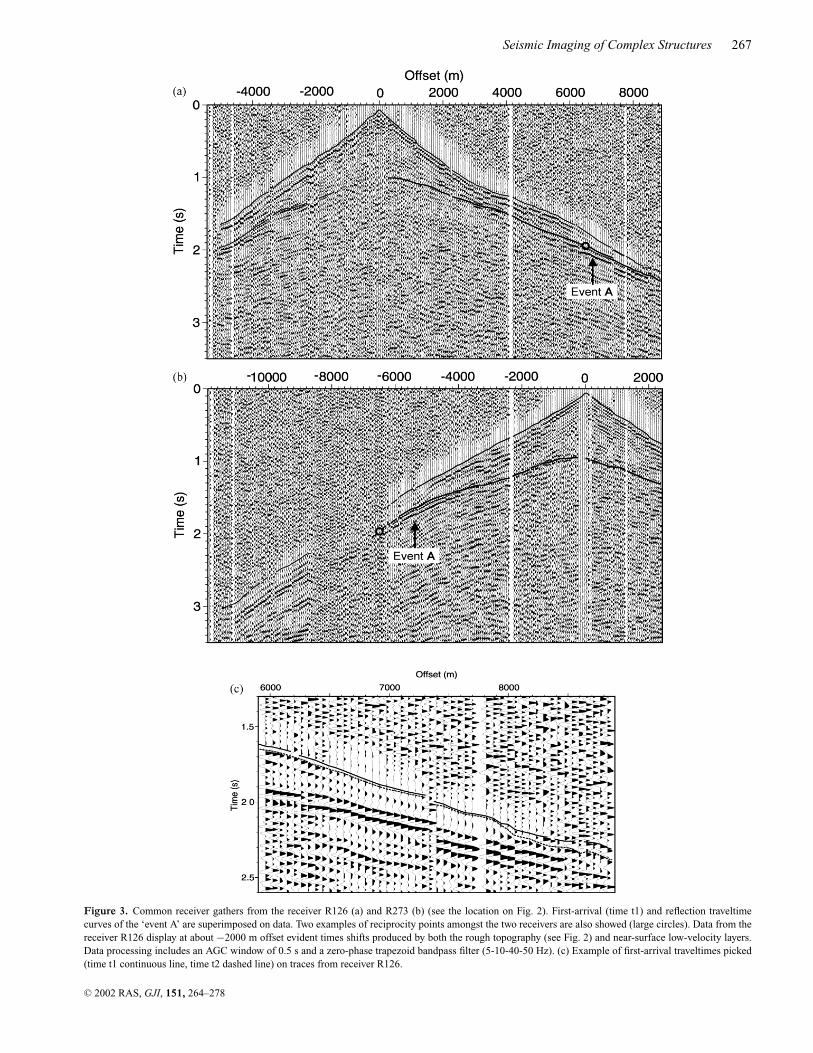
Fig. 3 displays two representative examples of automatic gaincontrol (AGC) processed sections, which exhibit a relatively highsignal-to-noise ratio and a good phase coherence even at large off-sets. However, seismic data suffer from high frequency time jittersrelated to the rough topography and to near-surface lateral velocitychanges. First arrivals are clear up to 5000–6000 m; moving to-wards larger offsets, refracted energy strongly decreases and largeamplitude wide-angle reflections are evident.

First arrivals were sampled following a picking strategy whichis based on the readings of a time window (t1, t2) bracketing thepresumed traveltime instead of a single pick with a weighting factor(Herrero et al. 1999). The time t2 is the upper limit for the expectedfirst-arrival and the time t1 (smaller than t2) is the time at whichtraces show a change in the signal coherence, amplitude standout andwaveform character which suggests that the first-arrival is includedbetween the time window t1–t2 (Fig. 3c). The width of the t1–t2window provides a criterion for data weighting during the inversion.When it is possible to pick only the time t2 owing to a low signal-to-noise ratio, this information is also taken into account during theinversion, since accepted models must provide theoretical arrivaltimes smaller than the measured t2.

Over 6400 first-arrival times were handpicked on 32 record sec-tions. These sections were selected based on the clarity of first-arrivals and the receiver locations along the profile, in order to en-sure homogeneous data coverage (Fig. 2). The maximum offset fordetecting first arrivals ranges from 8000 m to 13 000 m. Very clearimpulsive first arrivals, observed up to about 4000 m offset, wereassigned a t1–t2 window of 0.01 s, which is equal to a quarter ofthe dominant period. At larger offsets, the estimated width of t1–t2window ranges from 0.02 to 0.08 s depending on the offset (Fig. 3c).

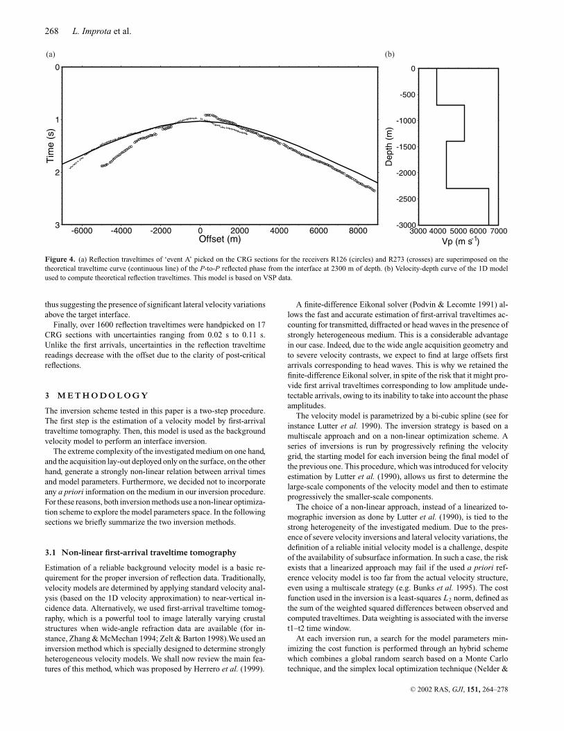
Concerning the reflection phases, the most noticeable featuresare large amplitude wide-angle reflections, which display an excel-lent phase coherence and lateral continuity at offsets larger than5000 m on many CRG record sections (‘event A’ in Figs 3a and b).In order to correlate the observed reflections to geological disconti-nuities known from well data, we computed the expected reflectiontravel times in a 1D velocity model inferred from VSP data (Fig. 4).The theoretical traveltime curves suggest that these large ampli-tude events may be interpreted as post-critical reflections from afirst-order crustal discontinuity drilled at a depth of about 2300 m(1250 mbsl), the latter representing a target for the seismic explo-ration in the survey area.

However, due to the presence of many reflection events on eachrecord section in the wide-angle offset range, the consistent identi-fication of ‘event A’ is problematic especially in regions with lowsignal-to-noise ratio. In order to ensure a correct phase identifica-tion, we took advantage of data redundancy and used reciprocityrelationships between CRG record sections (Fig. 3).

On the other hand, within the near-vertical offset range, the signal-to-noise ratio is low and no clear and continuous near-vertical inci-dence events appear (Fig. 3). In order to identify ‘event A’ at smalloffsets, we also analysed data arranged in Common Mid-Point gath-ers (CMP), this data arrangement being more suitable to study near

C© 2002 RAS, GJI, 151, 264–278

266 L. Improta et al.

5km0 2.5

1 2 34 5 8 96 7

N

Figure 1. Tectonic setting of the wide-angle seismic experiment. (1) Plio-Pleistocene clastic deposits, (2) Cenozoic clayey sediments; (3) Mesozoic basinalrocks; (4) normal faults; (5) thrusts; (6) synclines; (7) anticlines; (8) seismic profile; (9) well for oil exploration.

Figure 2. Topography along the seismic profile and location of the receivers used for the transmission tomography (stars).

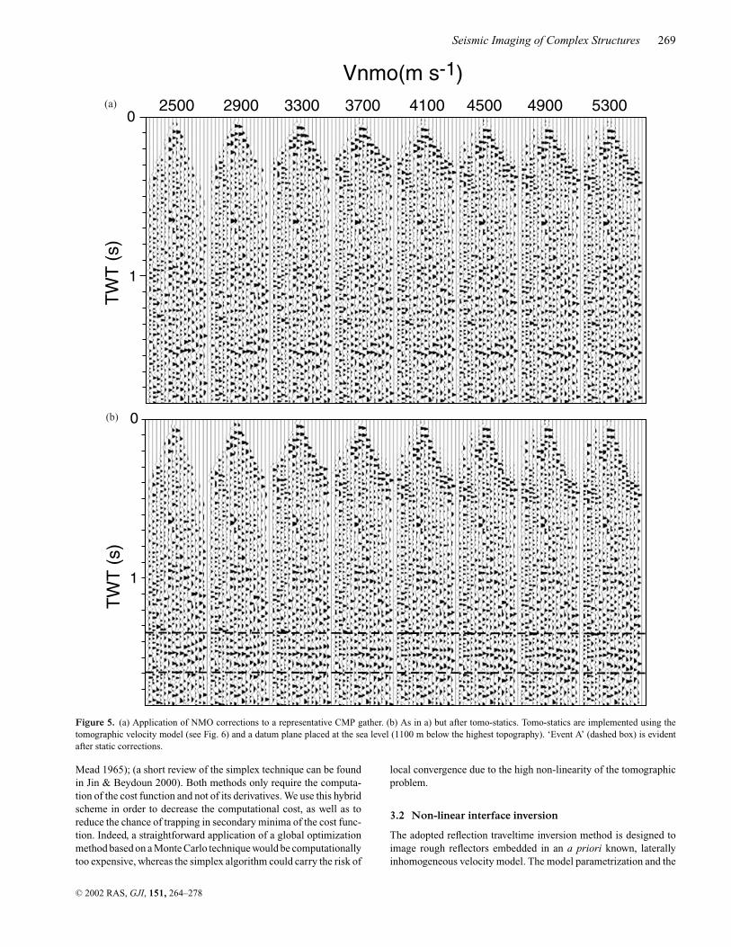
vertical-reflections. The application of tomo-statics (tomographyplus static corrections; Zhu et al. 1992) and of the CVS (ConstantVelocity Stack) method favoured identification and picking of ‘eventA’ at offset smaller than 4000 m on several CMP gathers (Fig. 5).

These reflection traveltime picks were then used as constraints (inaddition to reciprocity relationships) for the identification of ‘eventA’ on CRG sections. It is interesting to note that the normal move-outvelocities estimated for ‘event A’ range from 3000 to 4600 m s−1,

C© 2002 RAS, GJI, 151, 264–278


Figure 3. Common receiver gathers from the receiver R126 (a) and R273 (b) (see the location on Fig. 2). First-arrival (time t1) and reflection traveltimecurves of the ‘event A’ are superimposed on data. Two examples of reciprocity points amongst the two receivers are also showed (large circles). Data from thereceiver R126 display at about −2000 m offset evident times shifts produced by both the rough topography (see Fig. 2) and near-surface low-velocity layers.Data processing includes an AGC window of 0.5 s and a zero-phase trapezoid bandpass filter (5-10-40-50 Hz). (c) Example of first-arrival traveltimes picked(time t1 continuous line, time t2 dashed line) on traces from receiver R126.

C© 2002 RAS, GJI, 151, 264–278


(a) (b)

-1

Figure 4. (a) Reflection traveltimes of ‘event A’ picked on the CRG sections for the receivers R126 (circles) and R273 (crosses) are superimposed on thetheoretical traveltime curve (continuous line) of the P-to-P reflected phase from the interface at 2300 m of depth. (b) Velocity-depth curve of the 1D modelused to compute theoretical reflection traveltimes. This model is based on VSP data.

thus suggesting the presence of significant lateral velocity variationsabove the target interface.

Finally, over 1600 reflection traveltimes were handpicked on 17CRG sections with uncertainties ranging from 0.02 s to 0.11 s.Unlike the first arrivals, uncertainties in the reflection traveltimereadings decrease with the offset due to the clarity of post-criticalreflections.

3 M E T H O D O L O G Y

The inversion scheme tested in this paper is a two-step procedure.The first step is the estimation of a velocity model by first-arrivaltraveltime tomography. Then, this model is used as the backgroundvelocity model to perform an interface inversion.

The extreme complexity of the investigated medium on one hand,and the acquisition lay-out deployed only on the surface, on the otherhand, generate a strongly non-linear relation between arrival timesand model parameters. Furthermore, we decided not to incorporateany a priori information on the medium in our inversion procedure.For these reasons, both inversion methods use a non-linear optimiza-tion scheme to explore the model parameters space. In the followingsections we briefly summarize the two inversion methods.

3.1 Non-linear first-arrival traveltime tomography

Estimation of a reliable background velocity model is a basic re-quirement for the proper inversion of reflection data. Traditionally,velocity models are determined by applying standard velocity anal-ysis (based on the 1D velocity approximation) to near-vertical in-cidence data. Alternatively, we used first-arrival traveltime tomog-raphy, which is a powerful tool to image laterally varying crustalstructures when wide-angle refraction data are available (for in-stance, Zhang & McMechan 1994; Zelt & Barton 1998).We used aninversion method which is specially designed to determine stronglyheterogeneous velocity models. We shall now review the main fea-tures of this method, which was proposed by Herrero et al. (1999).

A finite-difference Eikonal solver (Podvin & Lecomte 1991) al-lows the fast and accurate estimation of first-arrival traveltimes ac-counting for transmitted, diffracted or head waves in the presence ofstrongly heterogeneous medium. This is a considerable advantagein our case. Indeed, due to the wide angle acquisition geometry andto severe velocity contrasts, we expect to find at large offsets firstarrivals corresponding to head waves. This is why we retained thefinite-difference Eikonal solver, in spite of the risk that it might pro-vide first arrival traveltimes corresponding to low amplitude unde-tectable arrivals, owing to its inability to take into account the phaseamplitudes.

The velocity model is parametrized by a bi-cubic spline (see forinstance Lutter et al. 1990). The inversion strategy is based on amultiscale approach and on a non-linear optimization scheme. Aseries of inversions is run by progressively refining the velocitygrid, the starting model for each inversion being the final model ofthe previous one. This procedure, which was introduced for velocityestimation by Lutter et al. (1990), allows us first to determine thelarge-scale components of the velocity model and then to estimateprogressively the smaller-scale components.

The choice of a non-linear approach, instead of a linearized to-mographic inversion as done by Lutter et al. (1990), is tied to thestrong heterogeneity of the investigated medium. Due to the pres-ence of severe velocity inversions and lateral velocity variations, thedefinition of a reliable initial velocity model is a challenge, despiteof the availability of subsurface information. In such a case, the riskexists that a linearized approach may fail if the used a priori ref-erence velocity model is too far from the actual velocity structure,even using a multiscale strategy (e.g. Bunks et al. 1995). The costfunction used in the inversion is a least-squares L2 norm, defined asthe sum of the weighted squared differences between observed andcomputed traveltimes. Data weighting is associated with the inverset1–t2 time window.

At each inversion run, a search for the model parameters min-imizing the cost function is performed through an hybrid schemewhich combines a global random search based on a Monte Carlotechnique, and the simplex local optimization technique (Nelder &

C© 2002 RAS, GJI, 151, 264–278


0

1

2500 41003300 37002900 4500 53004900

Vnmo(m s-1)

0

1

(a)

(b)

Figure 5. (a) Application of NMO corrections to a representative CMP gather. (b) As in a) but after tomo-statics. Tomo-statics are implemented using thetomographic velocity model (see Fig. 6) and a datum plane placed at the sea level (1100 m below the highest topography). ‘Event A’ (dashed box) is evidentafter static corrections.

Mead 1965); (a short review of the simplex technique can be foundin Jin & Beydoun 2000). Both methods only require the computa-tion of the cost function and not of its derivatives. We use this hybridscheme in order to decrease the computational cost, as well as toreduce the chance of trapping in secondary minima of the cost func-tion. Indeed, a straightforward application of a global optimizationmethod based on a Monte Carlo technique would be computationallytoo expensive, whereas the simplex algorithm could carry the risk of

local convergence due to the high non-linearity of the tomographicproblem.

3.2 Non-linear interface inversion

The adopted reflection traveltime inversion method is designed toimage rough reflectors embedded in an a priori known, laterallyinhomogeneous velocity model. The model parametrization and the

C© 2002 RAS, GJI, 151, 264–278


forward traveltime modelling used in the interface inversion arebased on a method proposed by Amand & Virieux (1995).

The reflection traveltime for a source–receiver pair and for a giveninterface is computed by a three-step procedure. Initially, first arrivaltraveltimes from each source and receiver to the nodes of a regulargrid are computed by the fast time estimator of Podvin & Lecomte(1991). These traveltimes are computed in the background velocitymodel and stored in time tables. Then, based on the time tables,the one-way traveltimes for a source–receiver pair to each point of agiven interface are computed performing an interpolation among thenearest four grid nodes. Finally, according to Fermat’s principle, thereflection point for a source–receiver pair and for a given interfacewill be the one providing the minimum total traveltime.

A bi-cubic spline, interface model parametrization is used(Virieux & Farra 1991). The interface nodes are equally spacedat fixed horizontal locations and can move vertically with continu-ity within a given depth range. The cost function is a least squaresL2 norm, defined as the sum of the weighted squared differencesbetween observed and theoretical traveltimes. Similarly to the first-arrival inversion method, the inversion strategy follows a multiscaleapproach and employs a non-linear optimization technique (a mod-ified version of the simplex technique proposed by Nelder & Mead1965). A series of inversions is run by progressively increasing thenumber of interface position nodes, as done by Lutter & Nowack(1990). At each inversion run, we generate the vertices (starting in-terface models) of the initial simplex by randomly perturbing in agiven depth range the minimum cost interface model obtained inthe previous run. The smaller is the spacing of the interface nodes,the smaller is the used depth range.

4 2 D B A C KG RO U N D V E L O C I T YM O D E L

Over 6400 first arrivals were used to determine a background veloc-ity model by the traveltime tomography. The application to highlyredundant data makes the inversion process very stable and robustand allows for a reliable and an accurate model building.

In order to avoid border effects, the model was extended 1000 msouthwestward of the first source and 800 m northeastward of thelast one. No a priori information about the model was used. Trav-eltimes were computed by a regular grid with a 50 × 50 m spacing.A succession of four inversions was run by inverting 12-, 32-, 96-and 128-node models. Each inversion run was halted as soon asthe cost function stopped decreasing during the last 5000 iterations.In all the performed runs, a smaller minimum of the cost functionwas reached by increasing the number of velocity nodes. Runningthe 128-node inversion, we obtained a final velocity model that ischaracterized by a RMS traveltime residual of 0.04 s (close to theaverage uncertainty in time reading).

The final 128-node model (16 horizontal nodes and 8 verticalnodes corresponding to a node spacing of 1000 × 537 m) (Fig. 6a)has small first-arrival time residuals confined in the ±0.03 s timerange (Fig. 6d). Larger residuals, up to 0.07 s, are occasionallyobserved at offsets smaller than 500 m; they are caused by near-surface small-scale features which are not well modelled due to thepoor spatial resolution.

The model resolution was studied by an a posteriori checkerboardtest (Hearn & Ni 1994). The perturbation added to the final tomo-graphic image in order to obtain the checkerboard model consistsof a 16×8 cells pattern with a maximum perturbation of ±50 m s−1

(Fig. 6b). Such a small amount of perturbation is chosen in order to

avoid changing the wave path in the medium. The inversion proce-dure is then applied to synthetic first-arrival times computed for thecheckerboard model. Fig. 6(c) displays the recovered perturbationpattern, which is obtained by subtracting, point by point, the refer-ence and the retrieved checkerboard models. This image gives directinformation on how data and the method used are spatially sensi-tive to the shape and amplitude of small velocity perturbations inthe final tomographic image. A quantitative assessment of the spa-tial resolution is obtained by measuring the local cross-correlationbetween the know and recovered checkerboard model around eachnode. This approach is similar to the one proposed by Zelt (1998),which is based on a semblance function. The best resolved region(with a correlation larger than 0.5) extends from the surface to about1400–1800 mbsl. between 5000–12 000 m. Resolution progres-sively deteriorates with depth and is low on both sides of the model,where the perturbation pattern is not retrieved at depths larger than500–1000 mbsl.

The final model displays significant lateral and vertical velocityvariations. A broad anticlinal isovelocity feature is evident between8500 and 12 000 m from the surface down to about 500 mbsl. Insidethe anticlinal structure, a high velocity (5000–5300 m s−1) regionis broken off by a vertical velocity inversion placed at about 200mbsl, thus grading into a low velocity (4600–5000 m s−1) region.On the eastern flank of the anticlinal feature, an abrupt deepen-ing of the 3750–4500 m s−1 isovelocity lines occurs. Conversely,to the west, the anticlinal structure blends into a near surface syn-clinal feature with velocities ranging from 2000 to 3500 m s−1.A sharp velocity increase from 5000–5500 m s−1 up to 6000 ms−1 is evident between 6000 and 11 000 m at depths larger than1500–2000 mbsl.

5 A P P L I C AT I O N O F T H E I N T E R FA C EI N V E R S I O N T O ‘ E V E N T A’

Over 1600 near-vertical/wide-angle reflection traveltimes of ‘eventA’ were used to the test the interface inversion method previously de-scribed. The one-way traveltime tables were computed by a squaredgrid with a 50 m spacing and the 128-node velocity model wasused as background reference medium. Reflection traveltimes wereweighted by a factor that inversely depends on the uncertainty in thearrival time reading.

A succession of five interface models parametrized by 2, 3, 5,9 and 17 nodes were progressively inverted (Fig. 7). Moving froma small to a larger number of interface position nodes we alwaysobserved a decrease of the final value of the cost function. Theinversion procedure stopped after the fifth run, since the RMS forthe minimum cost 17-node model (0.07 s) was close to the averageerror on arrival time readings (0.06 s).

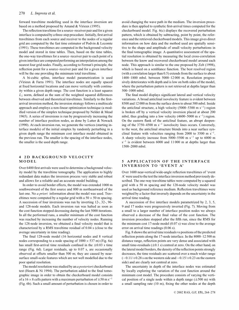
Fig. 8 shows the arrival time residuals vs positions of the predictedreflection points along the 17-node interface. In the 8000–12 500 mdistance range, reflection points are very dense and associated withsmall time-residuals (±0.1 s) centred at zero. On the other hand, onthe lateral model borders, the density of the reflection points stronglydecreases, the time residuals are scattered over a much wider range(−0.11/+0.28 s on the western side and −0.15/+0.23 on the easternside) and are clearly not centred at zero.

The uncertainty in depth of the interface nodes was estimatedby locally exploring the variation of the cost function around theminimum cost model. The procedure consists of varying the verti-cal position of a single node within a depth range (±500 m) witha small sampling rate (10 m), fixing the other nodes at the depth

C© 2002 RAS, GJI, 151, 264–278


(a)

(b)

(c)

(d)

Figure 6. (a) The final velocity model determined by first-arrival traveltime tomography. This model is parametrized by 128 nodes (black solid circles). Thebest resolved region of the model extends from the topographic surface down to the black dashed line. The well location is showed. (b) Perturbation patternused to perform the checkerboard resolution test. The perturbation consists of a 16 ×8 cell pattern with a maximum perturbation of ±50 m s−1 centred on eachnode. (c) Retrieved perturbation pattern. (d) First-arrival time residuals for two representative CRG sections. The time residuals are computed for both timest1 and times t2. The receiver positions are depicted by triangles.

C© 2002 RAS, GJI, 151, 264–278


3-node

17-node

9-node

5-node

2-node

Figure 7. Minimum cost interface models obtained by performing a succession of five inversion runs with an increasing number of interface nodes (graysolid circles). The interface inversion technique is applied to over 1600 reflection traveltime of ‘event A’ picked for the receiver (stars) and source (triangles)displayed in the lower panel. The background reference medium used to compute reflection traveltimes is showed in Fig. 6(a).

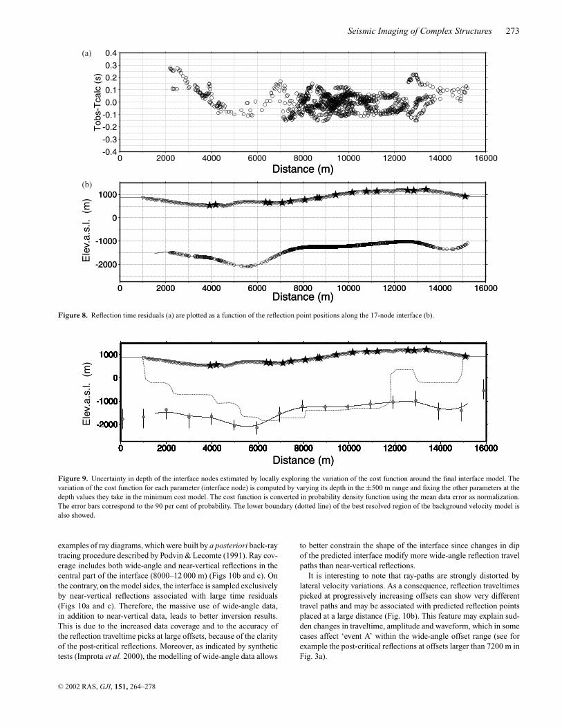
values they have in the minimum cost model. The variation of thecost function is computed for each parameter and converted in prob-ability density function using the mean data error as normalization.The uncertainty in depth of the nodes (Fig. 9) is clearly correlatedwith the time residuals (Fig. 8a), the density of the reflection points(Fig. 8b) and the background model resolution. Indeed, the best re-

solved part of the interface extends from 8000 to 12 000 m, whereaslarge uncertainties in the shape and location affect both sides of theinterface model.

It must be noted that errors on the position and shape of the inter-face also depend on the variability of the incidence angle range atthe reflection points along the interface. Figs 10(a)–(c) show three

C© 2002 RAS, GJI, 151, 264–278


Ele

v.a.

s.l.

(m)

(a)

(b)

Figure 8. Reflection time residuals (a) are plotted as a function of the reflection point positions along the 17-node interface (b).

Ele

v.a.

s.l.

(m)

Figure 9. Uncertainty in depth of the interface nodes estimated by locally exploring the variation of the cost function around the final interface model. Thevariation of the cost function for each parameter (interface node) is computed by varying its depth in the ±500 m range and fixing the other parameters at thedepth values they take in the minimum cost model. The cost function is converted in probability density function using the mean data error as normalization.The error bars correspond to the 90 per cent of probability. The lower boundary (dotted line) of the best resolved region of the background velocity model isalso showed.

examples of ray diagrams, which were built by a posteriori back-raytracing procedure described by Podvin & Lecomte (1991). Ray cov-erage includes both wide-angle and near-vertical reflections in thecentral part of the interface (8000–12 000 m) (Figs 10b and c). Onthe contrary, on the model sides, the interface is sampled exclusivelyby near-vertical reflections associated with large time residuals(Figs 10a and c). Therefore, the massive use of wide-angle data,in addition to near-vertical data, leads to better inversion results.This is due to the increased data coverage and to the accuracy ofthe reflection traveltime picks at large offsets, because of the clarityof the post-critical reflections. Moreover, as indicated by synthetictests (Improta et al. 2000), the modelling of wide-angle data allows

to better constrain the shape of the interface since changes in dipof the predicted interface modify more wide-angle reflection travelpaths than near-vertical reflections.

It is interesting to note that ray-paths are strongly distorted bylateral velocity variations. As a consequence, reflection traveltimespicked at progressively increasing offsets can show very differenttravel paths and may be associated with predicted reflection pointsplaced at a large distance (Fig. 10b). This feature may explain sud-den changes in traveltime, amplitude and waveform, which in somecases affect ‘event A’ within the wide-angle offset range (see forexample the post-critical reflections at offsets larger than 7200 m inFig. 3a).

C© 2002 RAS, GJI, 151, 264–278


Ele

v.a.

s.l.(

m)

Ele

v.a.

s.l.(

m)

Ele

v.a.

s.l.(

m)

(a)

(b)

(c)

Figure 10. (lower panel) Back ray-tracing of the modelled reflection phase (‘event A’) in the background velocity model and (upper panel) reflection timeresiduals for three receivers (stars) located in the left (a), central (b) and right part (c) of the seismic line.

C© 2002 RAS, GJI, 151, 264–278


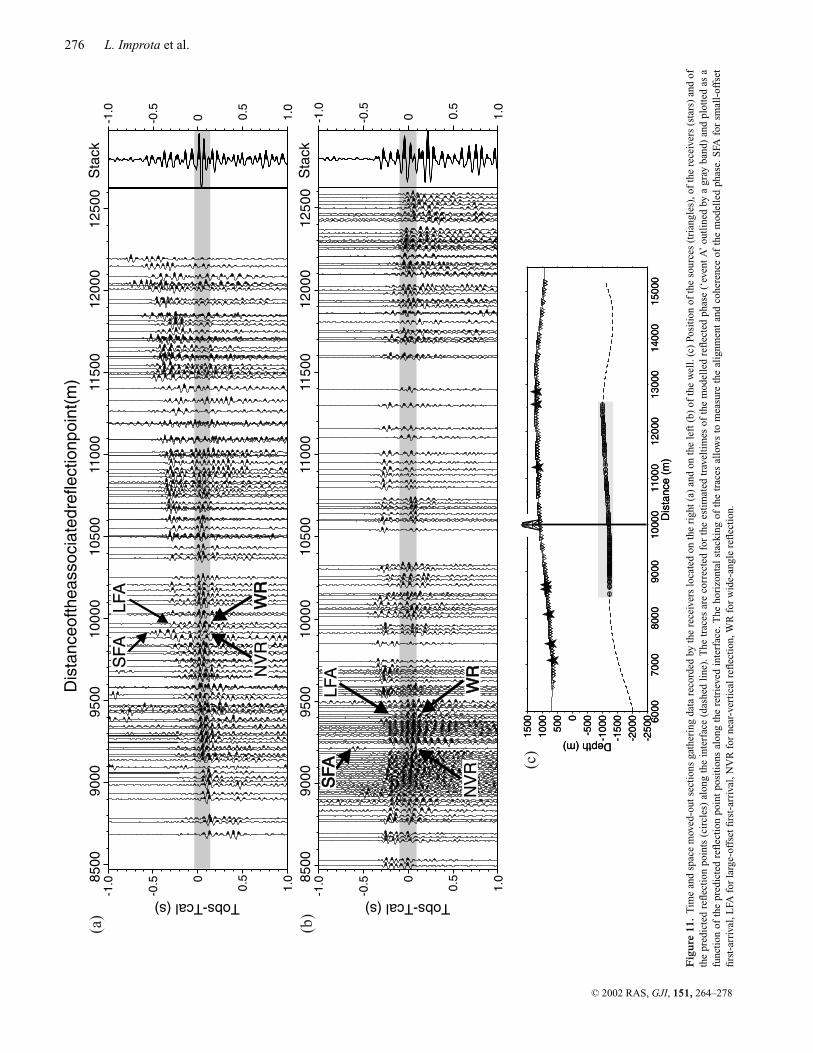
6 T I M E A N D O F F S E T M OV E - O U TO F ‘ E V E N T A’

The interface inversion method allows us to estimate the position ofthe reflection point along the minimum-cost interface model for eachmodelled traveltime. Therefore, the modelled data can be gatheredin new panels as a function of the predicted reflection point positionsand corrected for the computed reflection traveltime. This procedureis similar to a move-out scheme but using a laterally inhomogeneousbackground medium and a rough interface. In case of no error onlocation and shape of the interface, the modelled reflection eventsshould align at 0 s and should show a lateral coherence on themoved-out panels. Therefore, reliability of the determined interfacecan be verified by measuring the alignment of reflection events onthe moved-out gathers by an horizontal stacking of the traces.

Figs 11(a) and (b) show two examples of time and space moved-out gathers. These panels gather traces associated with reflectionpoints for distances comprised in the 8500–12 600 m range (wherethe interface is well resolved) (Fig. 11c). On the panel displayedin Fig. 11(a), which gathers data from the receivers located on theright side of the model, the alignment and coherence of ‘event A’are excellent for reflection point distances lower than 11 000 m.At larger distances, the phase alignment is less clear, the reflectionpoints being associated with weak near-vertical reflections pickedin regions with low signal-to-noise ratio (see for instance the near-vertical data showed in Fig. 3b). The phase alignment and coherenceare proved by the horizontal stacking of the traces, which clearlyshows a coherent signal at 0 s.

On the panel gathering the traces for receivers located on the leftside of the model (Fig. 11b), the alignment of ‘even A’ is evidentfor reflection point distances in the 8500–10 000 m range and largerthan 10 500 m. The horizontal stacking confirms a phase alignmentat about 0 s. In addition, it shows a further coherent signal at about−0.3 s, which results from the stacking of large amplitude first-arrivals for reflection point distances lower than 9500 m. This isnot surprising, since first-arrival pulses and ‘event A’ often displaysimilar apparent velocities on CRG sections in the intermediate(3000–6000 m) offset range (Fig. 3a).

It is interesting to note that both near-vertical (NVR) and wide-angle reflections (WR) associated with nearby reflection points alignon the panels displayed in Figs 11(a) and (b). This is an a poste-riori validation of the velocity model reliability. Indeed, given thedifferent travel path of the near-vertical and wide-angle reflections,only an accurate velocity model would produce an alignment of thereflection events, whatever offset data are used.

7 C O M PA R I S O N W I T H V S P DATA

The obtained velocity and interface models were compared to VSPdata acquired on the seismic line (Fig. 1). As the VSP sampling(20 m) was largely smaller than the vertical node spacing of thevelocity model (537 m), the VSP profile was low-pass filtered(λ < 1 km) in order to cut-off the small-scale components which cannot be solved by the tomographic inversion (Fig. 12). The velocity-depth curve inferred by the tomographic model matches well the fil-tered VSP profile from the surface to about 2400 mbgl (1300 mbsl).At larger depth, where resolution of the background model is low(Fig. 6c), the agreement between the two velocity-depth curves pro-gressively decreases.

VSP data fully confirm the interface inversion results. Indeed,the depth difference between the retrieved interface and the sharp

first-order velocity contrast associated with the target discontinuity(drilled at about 1250 mbsl) is about 40 m.

Surface geology and well information allow to associate featuresof the velocity model with geological units. The broad anticlinalisovelocity feature imaged from 8500 to 12 000 m (Fig. 6a) is inagreement with the antiform mapped in Fig. 1. The well, which ex-plored this structure, drilled a system of thrusts involving Mesozoicbasinal rocks: two thrust sheets, mainly composed of high veloc-ity (5200–5500 m s−1) cherty limestones, overlay tectonically at300 mbsl a succession of shales and cherts characterized by lowerseismic velocities (Fig. 12). Therefore, on the basis of well data, thehigh velocity (5000–5300 m s−1) region located inside the anticli-nal feature and the underlying low velocity (4600–5000 m s−1) layermay be associated with the limestone thrusts and with shaley/chertystrata, respectively. Moreover, the abrupt deepening of the isove-locity lines on the eastern flank of the antiform, is indicative ofthe thrust structure and correlates with the surface outcropping ofa thrust ramp eastward of the seismic line. To the west, the near-surface synclinal isovelocity feature is in agreement with a synformfilled by Cenozoic clays and Pliocene sands. In addition, the deep-ening of the 2000–3000 m s−1 isovelocity lines at about 6000 mmatches well the NW–SE trending axis of the syncline.

The interface determined by reflection traveltimes inversion maybe associated with the top of a cherty limestone succession. Thisinterpretation, that is locally proved by well information, may beextended to the 6000–11000 m distance range, where the retrievedreflector follows the top of the high velocity (5500–6000 m s−1)region imaged by tomography (Fig. 6a) and the velocity model res-olution is high (Fig. 6c).

8 D I S C U S S I O N A N D C O N C L U S I O N S

In this paper, we tested a two-step procedure for the separate in-version of first arrival and reflection traveltimes with a multi-foldwide-angle data set. Transmission tomography is used to determinea smooth velocity model, which is then employed as the backgroundreference medium for a subsequent interface inversion. This proce-dure is specially designed to image rough reflectors embedded instrongly inhomogeneous media by modelling dense data (acquiredwith a wide-angle geometries) and is able to operate with a roughtopography, unevenly spaced data and in presence of severe lateraland vertical velocity variations.

Both inversion methods employ a fast technique for the forwardproblem solution based on the finite-difference Eikonal solver ofPodvin & Lecomte (1991). The speed in the forward problem solu-tion favours the use of an inversion strategy to perform a massiveexploration of the model parameters (velocity or interface positionnodes). The strategy for model space exploration, which is similarfor both inversion techniques, is based on a multiscale approach andon a non-linear optimization scheme. The choice of a non-linear ap-proach is tied to the high degree of non-linearity between arrivaltraveltimes and model parameters, due both to the strong hetero-geneity of the investigated medium and to the acquisition lay-out,which is deployed only on the surface. The incorporation of a non-linear optimization scheme into a multiscale approach makes themodel parameters estimation more stable and robust, reducing therisk of local convergence.

The testing with the wide-angle data set collected in the South-ern Apennines (Italy) reveals the advantages of the applicationof this inversion procedure in an on-land thrust belt environment,where conventional near-vertical reflection seismic failed to provide

C© 2002 RAS, GJI, 151, 264–278


8500

1000

095

0090

0010

500

1250

012

000

1150

011

000

SFA

Dis

tanc

eofth

eass

ocia

tedr

efle

ctio

npoi

nt(m

)

NV

RW

RW

R

LFA

8500

1000

095

0090

0010

500

1250

012

000

1150

011

000

SFA

SFA

LFA

NV

RW

RW

R

(a)

(b)

(c)

Fig

ure

11.

Tim

ean

dsp

ace

mov

ed-o

utse

ctio

nsga

ther

ing

data

reco

rded

byth

ere

ceiv

ers

loca

ted

onth

eri

ght(

a)an

don

the

left

(b)

ofth

ew

ell.

(c)

Posi

tion

ofth

eso

urce

s(t

rian

gles

),of

the

rece

iver

s(s

tars

)an

dof

the

pred

icte

dre

flec

tion

poin

ts(c

ircl

es)

alon

gth

ein

terf

ace

(das

hed

line

).T

hetr

aces

are

corr

ecte

dfo

rth

ees

tim

ated

trav

elti

mes

ofth

em

odel

led

refl

ecte

dph

ase

(‘ev

ent

A’

outl

ined

bya

gray

band

)an

dpl

otte

das

afu

ncti

onof

the

pred

icte

dre

flec

tion

poin

tpo

siti

ons

alon

gth

ere

trie

ved

inte

rfac

e.T

heho

rizo

ntal

stac

king

ofth

etr

aces

allo

ws

tom

easu

reth

eal

ignm

ent

and

cohe

renc

eof

the

mod

elle

dph

ase.

SFA

for

smal

l-of

fset

firs

t-ar

riva

l,L

FAfo

rla

rge-

offs

etfi

rst-

arri

val,

NV

Rfo

rne

ar-v

erti

calr

eflec

tion

,WR

for

wid

e-an

gle

refl

ecti

on.

C© 2002 RAS, GJI, 151, 264–278


Figure 12. Comparison of the inversion results with well information. (1) shales (Lower Cretaceous); (2) cherts (Jurassic-Upper Triassic); (3) cherty limestones(Upper Triassic); (4) sandstones (Middle-Lower Triassic); (5) main thrust planes; (6) velocity-depth profile determined by VSP data; (7) low-pass (λ > 1000 m)filtered VSP velocity-depth profile; (8) velocity-depth curve inferred by the 2D tomographic model.

good-quality images because of the complexity of the velocity fieldand of a rough topography (Dell’Aversana 2001).

The use of dense large offset refraction data, which contain rel-evant information on the velocity distribution in depth, along withthe use of a robust non-linear inversion technique for velocity opti-mization, enabled us to produce a detailed and reliable tomographicmodel down to a maximum depth of 2500–3000 m from the surface(Figs 6a and c). Despite the extreme complexity of the investigatedstructure, which also includes severe velocity inversions, this modelis consistent with the VSP data (Fig. 12) and clearly outlines anti-clinal and synclinal structures.

The availability of an accurate laterally inhomogeneous velocitymodel, subsequently enabled us to take advantage of the relevantinformation carried by post-critical reflections (dominant in ampli-tude in the wide-angle offset range). This was performed by an inter-

face inversion of reflection traveltimes picked in the complete offsetrange. The inversion results, which are consistent with well informa-tion (Fig. 12), and synthetic tests (Improta et al. 2000), show that theuse of redundant wide-angle data in addition to near-vertical reflec-tions allows to reduce the uncertainty in the interface detection. Inaddition to the increased data coverage, the wide-angle componentsheavily contribute to the robustness of the inversion for two furtherreasons: (a) post-critical reflections picks are usually affected bysmall uncertainties due to the clarity of the events, (b) wide-angledata provide additional constraints on the interface shape, since achange in dip of the predicted interface strongly modifies the travelpath and arrival time of wide-angle reflections. These advantagesbecome evident in thrust belt regions, where the collection of highquality data by near-vertical seismic experiments may be a difficulttask.

C© 2002 RAS, GJI, 151, 264–278


In addition, as the topography is directly included in the interfaceinversion, no static corrections are required. This is a great advan-tage considering that the theoretical and practical extension of themethods for static computation to thrust belt regions with ruggedterrain remains a challenge (Schneider et al. 1995; Bevc 1997; Zhuet al. 1998). To sum up, our applications demonstrate that the inver-sion procedure can be efficient for target-orientated studies of theupper crust in complex geological environments, such as in thrustbelts.

Of course, the method suffers from some limitations. First, as theaccuracy of the background model has a strong influence on theinterface inversion results, the target-zone is limited in depth tothe best resolved region of the velocity model, whose lower bound-ary critically depends on the maximum offsets for usable refractedenergy. In our case, due to the low resolution of the velocity modelfor depths larger than 2500–3000 mbgl, the potential target-zone islimited to the shallow crust. A possible strategy to overcome thislimitation is to enlarge the spread of the acquisition geometry inorder to increase the exploration depth of the transmission tomog-raphy. This strategy was successfully used by Dell’Aversana et al.(2001) in a wider-angle survey performed recently in the SouthernApennines. Indeed, a detailed velocity model was produced downto a depth of 5000 mbgl by applying transmission tomography toredundant refracted data collected up to 25 000 m offset.

Another limitation of the procedure is the non-negligible humanintervention required to pick reflection traveltimes. In order to avoidthis limitation and to improve the time performance of the wholeprocedure, our future efforts will focus on the use of a differentobjective function in the interface inversion based on coherencemeasures. A possible approach could be based on the measure ofthe alignment of the target events on time and space moved-outpanels (see Section 6) by data staking. Besides, this improvementin time performance would facilitate the theoretical and practicalextension of the inversion procedure to 3D wide-angle data set.

A C K N O W L E D G M E N T S

We would like to thank Sergio Morandi of Enterprise Oil Italianafor his support and suggestions. The very useful comments and En-glish reviewing of C. Piromallo and S. Nielsen are greatly acknowl-edged. We acknowledge two anonymous reviewers and Prof. RoulHadoruege. This study has been financially supported by EnterpriseOil Italiana.

R E F E R E N C E S

Amand, P. & Virieux, J., 1995. Non linear inversion of synthetic seismicreflection data by simulated annealing, 65th Ann. Internat. Mtg: Soc. Expl.Geophy. Expanded Abstracts, 612–615.

Bevc, D., 1997. Flooding the topography: Wave equation datuming of landdata with rugged acquisition topography, Geophysics, 62, 1558–1569.

Bunks, C., Saleck, F.M., Zaleski, S. & Chavent, G., 1995. Multiscale seismicwaveform inversion, Geophysics, 60, 1457–1473.

Dell’Aversana, P., 2001. Integration of seismic, MT, and gravity data in athrust belt interpretation, First Break, 19, 335–341.

Dell’Aversana, P., Ceragioli, E., Morandi, S. & Zollo, A., 2000. A simulta-

neous acquisition test of high density “global offset” seismic in complexgeologicalal settings, First Break, 18, 87–96.

Dell’Aversana, P., Zucconi, V. & Colombo, D., 2001. Improvement in seismicacquisition by 3D Global offset approach, 71st Ann. Internat. Mtg: Soc.Expl. Geophy. Expanded Abstracts, 29–32.

Hearn, T.M. & Ni, J.F., 1994. Pn velocities beneath continental collisionzones, Geophys. J. Int., 117, 273–283.

Herrero, A., Zollo, A. & Virieux, J., 1999. 2D Non linear first arrival timeinversion applied to Mt. Vesuvius active seismic data (TomoVes96), Eur.Geophys. Soc.,, XXIV, General Assembly, 19–23 April, 1999, The Hague,The Netherlands.

Improta, L., Zollo, A., Frattini, M.R., Virieux, J., Herrero, A. &Dell’Aversana, P., 2000. Mapping interfaces in an overthrust re-gion by non-linear traveltime inversion of reflection data, Am.geophys. Un.,Fall Meeting, 15–19 December 2000, San Francisco,USA.

Jin, S. & Beydoun, W., 2000. 2D multiscale non-linear velocity inversion,Geophys. Prospect., 48, 163–180.

Jin, S. & Madariaga, R., 1994. Nonlinear velocity inversion by a two stepMonte Carlo method, Geophysics, 59, 577–590.

Kodaira, S., Takahashi, N., Nakanishi, A., Miura, S. & Kaneda, Y., 2000.Subducted seamount imaged in the rupture zone of the 1946 Nankaidoearthquake, Science, 289, 104–106.

Lynn, W.S. & Claerbout, J.F., 1982. Velocity estimation in laterally varyingmedia, Geophysics, 47, 884–897.

Lutter, W.J. & Nowack, R.L., 1990. Inversion of crustal structure using re-flections from the PASSCAL Ouachita Experiment, J. geophys. Res., 95,4633–4646.

Lutter, W.J., Nowack, R.L. & Braile, L.W., 1990. Seismic imaging of theupper crustal structure using travel times from the PASSCAL OuachitaExperiment, J. geophys. Res., 95, 4621–4631.

Mazzotti, A.P., Stucchi, E., Fradelizio, G.L., Zanzi, L. & Scandone, P., 2000.Seismic exploration in complex terrains: a processing experience in theSouthern Apennines, Geophysics, 65, 1402–1417.

Nelder, J.A. & Mead, R., 1965. A simplex method for function minimization,Comput J., 7, 308–313.

Podvin, P. & Lecomte, I., 1991. Finite difference computation of traveltimesin very contrasted velocity model: A massively parallel approach and itsassociated tools, Geophys. J. Int., 105, 271–284.

Samson, C., Barton, P.J. & Karwatowski, J., 1995. Imaging beneath anopaque basaltic layer using densely sampled wide-angle OBS, Geophys.Prospect., 43, 509–527.

Schneider, W.A., Phillip L.D. & Paal, E.F., 1995. Wave-equation velocityreplacement of the low velocity layer for overthrust-belt data, Geophysics,60, 573–579.

Virieux, J. & Farra, V., 1991. Ray tracing in 3D complex isotropic media:An analysis of the problem, Geophysics, 56, 2057–2069.

Zelt, C.A., 1998. Lateral velocity resolution from three-dimensional seismicrefraction data, Geophys. J. Int.,135, 1101–1112.

Zelt, C.A. & Barton, P.J., 1998. Three-dimensional seismic refraction to-mography: a comparison of two methods applied to data from the FaeroeBasin, J. geophys. Res., 103, 7187–7210.

Zelt, B.C., Talwani, M. & Zelt, C.A., 1998. Prestack depth migration ofdense wide-angle seismic data, Tectonophysics, 286, 193–208.

Zhang, J. & McMechan, G.A., 1994. 3D transmission tomography using wideaperture data for velocity estimation for irregular salt bodies, Geophysics,59, 1620–1630.

Zhu, X., Angstmon, B.G. & Sixta, D.P., 1998. Overthrust imaging withtomo-datuming: A case study, Geophysics, 63, 25–38.

Zhu, X., Sixta, D.P. & Angstman, B.G., 1992. Tomo-statics: Turning-raytomography + static corrections, The Leading Edge, 11, 15–23.

C© 2002 RAS, GJI, 151, 264–278

Seismic imaging of complex structures by non-linear traveltime inversion of dense wide-angle data:...

Documents

Transcript of Seismic imaging of complex structures by non-linear traveltime inversion of dense wide-angle data:...