
Dense Stereo Matching with Robust Cost Functions and ...
100
Ingenieurfakultät Bau Geo Umwelt Lehrstuhl für Methodik der Fernerkundung Dense Stereo Matching with Robust Cost Functions and Confidence-based Surface Prior Ke Zhu Vollständiger Abdruck der von der Ingenieurfakultät Bau Geo Umwelt Bauingenieur- und Vermessungswesen der Technischen Universität München zur Erlangung des akademischen Grades eines Doktor-Ingenieurs genehmigten Dissertation. Vorsitzender: Univ.-Prof. Dr. -Ing. Uwe Stilla Prüfer der Dissertation: 1. Univ.-Prof. Dr. -Ing. Richard Bamler 2. Hon.-Prof. Dr. -Ing. Peter Reinartz, Universität Osnabrück Die Dissertation wurde am 15.10.2013 bei der Technischen Universität München eingereicht und durch die Ingenieurfakultät Bau Geo Umwelt am 17.02.2014 angenommen.
-
Upload
khangminh22 -
Category
Documents
-
view
3 -
download
0
Transcript of Dense Stereo Matching with Robust Cost Functions and ...

Ingenieurfakultät Bau Geo Umwelt
Lehrstuhl für Methodik der Fernerkundung
Dense Stereo Matching with Robust Cost Functions and Confidence-based Surface Prior
Ke Zhu Vollständiger Abdruck der von der Ingenieurfakultät Bau Geo Umwelt Bauingenieur- und Vermessungswesen der Technischen Universität München zur Erlangung des akademischen Grades eines
Doktor-Ingenieurs genehmigten Dissertation.
Vorsitzender: Univ.-Prof. Dr. -Ing. Uwe Stilla Prüfer der Dissertation:
1. Univ.-Prof. Dr. -Ing. Richard Bamler 2. Hon.-Prof. Dr. -Ing. Peter Reinartz,
Universität Osnabrück
Die Dissertation wurde am 15.10.2013 bei der Technischen Universität München eingereicht und durch die Ingenieurfakultät Bau Geo Umwelt am 17.02.2014 angenommen.

I would like to dedicate this thesis to my loving parents, my wife and our child ...

Acknowledgements
I am grateful to Prof. Dr. Richard Bamler and Prof. Dr. Peter Reinartz for givingme the opportunity to carry out the thesis at TU-Munchen and in German AerospaceCenter (DLR). I also appreciate all their contributions of time, ideas, and suggestionsfor completing this thesis.
And I would like to express my heartfelt gratitude to Dr. Pablo d’Angelo for hiscontinued encouragement and invaluable suggestion throughout my doctoral researchstudy. I would like to acknowledge Dr. Daniel Neilson for the inspired and effectivecooperation during my IGSSE exchange at the University of Saskatchewan. I wouldlike to thank Dr. Matthias Butenuth for his goal-oriented supervision.

Abstract
The goal of dense stereo matching is to estimate the distance, or depth to an imagedobject in every pixel of an input image; this is achieved by finding pixel correspon-dences between the source image and one or more matching images. Applicationsthat make dense stereopsis active come from areas such as photogrammetry, remotesensing, mobile robotics, and intelligent vehicles. For instance, many remote sensingapplications require depth maps to generate digital elevation models from airborneand satellite imagery. There are hundreds, if not thousands, of approaches seekingto solve stereopsis. A number of factors that make computational stereopsis quitechallenging become apparent once one begins to use it in real-world applications;non-Lambertian reflectance, complex scene and radiometric changes, among otherfactors, are usually present in real-world data.
Dense stereo algorithms can be categorized into two methodologies based onthe way the problem is solved: Local and global. Local algorithms aim to solve theproblem via a local analysis at each input-image pixel, whereas global algorithmsformulate the stereopsis problem as one of finding an optimal solution to a globalenergy, or probability function. Developing a global stereo method considers threemain factors – calculation reliable observation to measure matching similarity, for-mulation of energy, or probability, function using additional priors, and optimizationof the global function to find the global extremum.
In this dissertation two methodical novelties are contributed – the merging strat-egy of match costs and the confidence-based surface prior incorporating a semiglobaloptimization framework. All dense stereo matching algorithms use match cost func-tions to measure the similarity between two pixels. In a real-world scenario, goodradiometric conditions are often disrupted by complicated and dynamic lightingsources, inappropriate camera configuration, and non-Lambertian reflectance of ob-jects. We investigate the interdependencies among matching performance, cost func-tions, and observation conditions using both close-range and remote-sensing data.Our cost-merging strategy combines the advantages of different match cost functionsand gives consideration to imagery configurations. In addition, a novel probabilisticsurface prior is introduced incorporating a new energy optimization method, callediSGM3. Our approach builds a probabilistic surface prior over the disparity spaceusing confidences on a set of reliably matched correspondences. Unlike many region-based methods, our method defines an energy formulation over pixels, instead ofregions in a segmentation; this results in a decreased sensitivity to the quality of theinitial segmentation. This dissertation suggests the way to developing robust stereomethods is on the level of obtaining costs and suitable energy formulation, and notonly the energy optimization. Both costs merging and the surface prior are generallyapplicable for almost all extended stereo methods.

Contents
Contents iv
Nomenclature vi
1 Introduction 11.1 Challenging Real-world Data . . . . . . . . . . . . . . . . . . . . . . . . . . . . . 41.2 Contributions . . . . . . . . . . . . . . . . . . . . . . . . . . . . . . . . . . . . . . 5
2 Dense Stereo Matching 82.1 Binocular Reconstruction . . . . . . . . . . . . . . . . . . . . . . . . . . . . . . . 92.2 Match Costs . . . . . . . . . . . . . . . . . . . . . . . . . . . . . . . . . . . . . . . 10
2.2.1 Match Cost Functions . . . . . . . . . . . . . . . . . . . . . . . . . . . . . 102.2.2 Spatial Cost Aggregation . . . . . . . . . . . . . . . . . . . . . . . . . . . 11
2.3 Local Stereo Algorithms . . . . . . . . . . . . . . . . . . . . . . . . . . . . . . . . 122.3.1 The Winner-takes-all Algorithm . . . . . . . . . . . . . . . . . . . . . . . 122.3.2 Other Algorithms . . . . . . . . . . . . . . . . . . . . . . . . . . . . . . . . 12
2.4 Global Stereo Algorithms . . . . . . . . . . . . . . . . . . . . . . . . . . . . . . . 132.4.1 MAP-MRF model for Stereo Matching . . . . . . . . . . . . . . . . . . . . 132.4.2 Energy Function Formulations . . . . . . . . . . . . . . . . . . . . . . . . 152.4.3 Methods for Optimization . . . . . . . . . . . . . . . . . . . . . . . . . . . 16
2.4.3.1 Mean Field Approximation . . . . . . . . . . . . . . . . . . . . . 162.4.3.2 Semi-Global Matching . . . . . . . . . . . . . . . . . . . . . . . . 17
2.5 Feature based Stereo Algorithms . . . . . . . . . . . . . . . . . . . . . . . . . . . 192.5.1 Edge-based Match Propagation . . . . . . . . . . . . . . . . . . . . . . . . 202.5.2 Efficient Large-Scale Stereo Matching . . . . . . . . . . . . . . . . . . . . 20
2.6 Summary . . . . . . . . . . . . . . . . . . . . . . . . . . . . . . . . . . . . . . . . 21
3 Robust Match Cost Functions for Dense Stereopsis 223.1 Related Work . . . . . . . . . . . . . . . . . . . . . . . . . . . . . . . . . . . . . . 233.2 Intensity, Color and Gradient . . . . . . . . . . . . . . . . . . . . . . . . . . . . . 243.3 Parametric Match Costs . . . . . . . . . . . . . . . . . . . . . . . . . . . . . . . . 253.4 Mutual Information . . . . . . . . . . . . . . . . . . . . . . . . . . . . . . . . . . 273.5 Non-Parametric Matching Costs . . . . . . . . . . . . . . . . . . . . . . . . . . . 283.6 Match costs merging . . . . . . . . . . . . . . . . . . . . . . . . . . . . . . . . . . 293.7 Summary . . . . . . . . . . . . . . . . . . . . . . . . . . . . . . . . . . . . . . . . 31
iv

CONTENTS
4 Probabilistic Pixel-wise Surface Stereo 334.1 Related Work . . . . . . . . . . . . . . . . . . . . . . . . . . . . . . . . . . . . . . 354.2 Hard Surface Constraints . . . . . . . . . . . . . . . . . . . . . . . . . . . . . . . 364.3 Confidence-Based Surface Prior . . . . . . . . . . . . . . . . . . . . . . . . . . . . 364.4 Energy Minimization via iSGM3 . . . . . . . . . . . . . . . . . . . . . . . . . . . 38
4.4.1 Obtaining Reliable Disparities . . . . . . . . . . . . . . . . . . . . . . . . 384.4.2 Robust Plane Fitting using Voting . . . . . . . . . . . . . . . . . . . . . . 384.4.3 Iterative SGM3 . . . . . . . . . . . . . . . . . . . . . . . . . . . . . . . . . 40
4.5 Summary . . . . . . . . . . . . . . . . . . . . . . . . . . . . . . . . . . . . . . . . 41
5 Results 445.1 Data Sets Used . . . . . . . . . . . . . . . . . . . . . . . . . . . . . . . . . . . . . 45
5.1.1 Middlebury Stereo Benchmark . . . . . . . . . . . . . . . . . . . . . . . . 455.1.2 DLR 3K Data Sets . . . . . . . . . . . . . . . . . . . . . . . . . . . . . . . 465.1.3 Satellite Stereo Pairs . . . . . . . . . . . . . . . . . . . . . . . . . . . . . . 47
5.2 Evaluation of Matching Cost Functions . . . . . . . . . . . . . . . . . . . . . . . 485.2.1 Methodology for Evaluation . . . . . . . . . . . . . . . . . . . . . . . . . . 495.2.2 Results on Middlebury Data Sets . . . . . . . . . . . . . . . . . . . . . . . 50
5.2.2.1 Results on Data without Radiometric Changes . . . . . . . . . . 505.2.2.2 Results on Data with Radiometric Changes . . . . . . . . . . . . 53
5.2.3 Results on Airborne Image Sequence . . . . . . . . . . . . . . . . . . . . . 605.2.4 Results on Satellite Data . . . . . . . . . . . . . . . . . . . . . . . . . . . 665.2.5 Discussion . . . . . . . . . . . . . . . . . . . . . . . . . . . . . . . . . . . . 69
5.3 Evaluation of the Confidence-based Surface Prior . . . . . . . . . . . . . . . . . . 705.3.1 Results on Middlebury Benchmark . . . . . . . . . . . . . . . . . . . . . . 705.3.2 Results on Airborne Stereo Pairs . . . . . . . . . . . . . . . . . . . . . . . 745.3.3 Discussion . . . . . . . . . . . . . . . . . . . . . . . . . . . . . . . . . . . . 75
5.4 Summary . . . . . . . . . . . . . . . . . . . . . . . . . . . . . . . . . . . . . . . . 77
6 Conclusion and Outlook 796.1 Outlook . . . . . . . . . . . . . . . . . . . . . . . . . . . . . . . . . . . . . . . . . 81
Appendix A: Data Set 82
References 84
v

Nomenclature
I An image.
Is, Im Source (reference) and match image1.
O Observation of a stereo pair, Is and Im.
p ∈ I Pixel p of image I.
I3→1 An intensity image with merged color channels.
5eI A gradient image derived in epiplar direction.
Seg Segmentation of a image.
δp Disparity at pixel p in a disparity map.
dp Disparity at pixel p in a plane map.
D Disparity range.
∆ Disparity map.
∆pl Plane-fit disparity map.
Πm A disparity plane with index m.
P(X) The prior probability of X.
P(X|Y ) The conditional probability of X, given Y.
P(X,Y ) The joint probability of X and Y.
α, β Scalar value.
ω Weight factor.
λ, κ Penalty factor.
1Without loss of generality, the left image is considered as the reference image. Is = IL and Im = IR.
vi

Chapter 1
Introduction
The goal of dense stereo matching is to estimate the distance, or depth, to an imaged objectin every pixel of an input image; this is achieved by finding pixel correspondences between thesource image and one or more matching images. The displacement between corresponding pixelsis then used to calculate depth, along with the relative position of the two cameras. Early stereoalgorithms used to extract features in different views, such as edges or corners, and identifythe similarities with features in the input images. In contrast, modern dense stereo algorithmsreconstruct scenes even with little texture where no features can be extracted.
Although it seems we can infer depth with our own eyes effortlessly, human depth perceptionis not able to estimate the distance of objects metrically. Computational dense stereo methodsperform the task by assigning a concrete depth to each pixel when enough parallax is present.Depth information is useful to understand scenes, and it enables higher-level image processingand information extraction. However, several factors make computational dense stereo hardin practice. Neighboring pixels may have the same intensity/color/local structure, leading tomatching ambiguities. Changing observation views causes occlusions that block part of oneimage from being seen in the other, and no depth can be estimated for these areas.
Broadly, dense stereo algorithms can be categorized into two methodologies based on the waythe problem is solved: local and global algorithms [Scharstein and Szeliski, 2002]. The most fun-damental component of every stereo algorithm is the match cost [Hirschmuller and Scharstein,2009]. All stereo methods include a cost function to measure the fitness of possible correspon-dences in a stereo pair. The match cost is an observation directly calculated from input images,and also called data term in an energy formulation. Local algorithms independently estimatecorrespondences for each pixel separately, without considering neighboring correspondences. Incontrast, global methods consider the neighborhood of each pixel using a regularization term,such as a smoothness assumption, or its belonging to a segment. Such an additional term addsprior knowledge and expectations to a depth map – for example, smooth surfaces, sharp edges,and scene visibility [Bleyer and Gelautz, 2005; Kolmogorov and Zabih, 2001; Szeliski et al.,2008]. In general, stereo matching is an ill-posed problem, so some regularization is required toachieve a meaningful solution. Moreover, the assumptions are often contradictory. In additionto smooth surfaces within objects, large discontinuities should remain at object boundaries. Theproblem is represented in a disparity map that leads to a global extreme of an energy functionconsisting of data and regularization terms defined over the whole image. This generally leads tocomputationally NP-hard 1 problems [Boykov et al., 2001; Kolmogorov and Zabih, 2001; Neilsonand Yang, 2008]. Different optimization methods are used to find the (approximated) extremum.
1Non-deterministic Polynomial-time hard
1

1. Introduction
In summary, developing a computational stereo method considers three main factors as shown inFigure 1.1: a) gaining reliable observation to measure matching similarity (cost computation); b)modelling goal function for the unknown solution with some prior assumptions (energy-functionformulation); c) achieving/approximating the global minimum (energy optimization).
Observation(Cost Calculation)
Application(Observation Conditions,
Observing Regions)
Solving(Energy Optimization)
Modelling(Energy Function Formulation)
Performing(Unknown Result)Global Methods Local Methods
Figure 1.1: Overview of the computational dense stereopsis. The three main factors fordeveloping a dense stereo method include obtaining reliable match costs, formulating solvableenergy function, and achieving/approximating the global extreme.
Applications that make the dense stereo active come from areas such as photogrammetry,mobile robotics, intelligent vehicles and remote sensing. For instance, many remote sensingapplications require depth maps to generate Digital Elevation Models (DEMs) from airborneand satellite imagery. DEMs are a fundamental dataset required for applications such as mobilephone network planning, flood prediction, and 3D city modeling and analysis [Jin et al., 2010; Juet al., 2009; Leberl et al., 2010; Zhang et al., 2011]. LiDAR 1 is often used for 3D reconstructionboth in close range and remote-sensing applications, but advanced dense stereopsis can be used inplace of LiDAR, resulting in models with higher resolution, improved application flexibility andlower operating cost [Kurz et al., 2012; Reinartz et al., 2010]. One application for fast, airborne3D reconstruction is damage evaluation and rescue support in the case of natural disasters, suchas land slides, as shown in Figure 1.2.
Unfortunately, the most recent stereo matching methods are developed using data sets withrelatively good radiometric configurations and small base lines. The observed scenes typicallycontain simple geometric figures. In contrast, real-world applications are more complex anddifficult than the widely-used benchmarks due to challenges in observation conditions and inthe features of the imaged objects. In remote-sensing applications, urban areas include highbuildings, slanted roofs and large homogenous regions. The light source is complex and dynamic– the sun instead of artificial ambient light sources. Most surfaces do not show a Lambertian-reflectance behavior, which leads to various image intensities of the same object point fromdifferent camera viewpoints. Moving cars, shadows of buildings and changing weather make datadynamic, even over a short period. Despite intense investigations by the research community inthe last decades, these challenges are not resolved and open problems remain.
This work introduces two methodological novelties which aim to be generally applicable
1Light Detection And Ranging
2

1. Introduction
Reference Images
Disparity Map
Scene Image
40
30
20
10
0
Figure 1.2: Airborne 3D Reconstruction after landslide in Doren, Austria. Top-right:Airborne stereo pair taken by DLRa 3K camera system using Canon EOS 1D Mark II cameras.Center: Disparity map generated by Top-right and colored with a heat scale such that colder(glue/violet) colors are closer to the camera than hotter (red/yellow) colors. Bottom-left: ascene image b from the similar view point of the visualization. Reconstructed region is assignedby a white frame.
aGerman Aerospace CenterbImage source: Gemeindedaten von Doren [www.statistik.at]
for almost all global optimization methods. 1) Based on the performance study of match costfunctions using both standard computer vision benchmarks and remote-sensing data, a mergingstrategy is introduced to design robust match costs. 2) A novel confidence-based surface prioris developed within a probabilistic framework. Depending on the reliability of the prior (theconfidence) from a previous matching, the introduced surface prior is modeled as a Gaussiandistribution, which can be probabilistically fused with the current approach. Moreover, weintroduce a new optimization framework in the energy space for iteratively updating/using theconfidence. Three data sets are used in this dissertation for benchmarking and evaluation ofthe developed methods: the Middlebury benchmark with radiometric changes, airborne imagesequences with an increasing baseline and satellite stereo pairs with large stereo angles.
This dissertation is structured as follows. In Chapter 2 we describe the dense stereo problemand existing methods for solving it. In addition, the influence and challenge of applied dataon matching performance are briefly discussed. The two main contributions of this dissertationare then methodically formulated. In Chapter 3, we introduce different match cost functions
3

1. Introduction
and the merging strategy to obtain robust costs. Chapter 4 presents the novel confidence-basedsurface prior and its relaxation in the global energy formulation. In Chapter 5, according tothe evaluation of different cost functions, we investigate the interdependencies among matchcost, matching performance, applied region and observation constraints. Moreover, we comparethe results with and without the proposed surface prior under a global energy formulation anddemonstrate that our approach has superior performance on all data sets used. Finally, weconclude our work in Chapter 6.
1.1 Challenging Real-world Data
There are hundreds approaches seeking to solve the stereopsis. A number of factors that makeit quite challenging become apparent once one begins to use it in real-world applications likemobile robotics and remote sensing. Non-Lambertian reflectance, complex scene, and radio-metric changes, among other factors, are usually present in real-world data. This leads to lowperformance of stereo algorithms that perform well on some de-facto standard benchmarks inthe computer vision community. With respect to real-world data, we have summarized thechallenges for stereo matching methods as follows:
Complicated radiometric conditions. Lighting sources in the real world including the sunand man-made sources, are complicated and dynamic. Even for close-up images, radio-metric changes can appear – for example, a cloud is covering the sun, the headlight of acar is turned on, and so on. In contrast, dense stereo algorithms are typically developedand evaluated using data with a small baseline configuration as well as artificial and oftenambient light sources. Radiometric changes due to, for example, vignetting and gammachanges, and so forth, are often simulated by modifying small baseline images [Hirschmullerand Scharstein, 2009; Scharstein and Szeliski, 2002]; but, these simulations do not captureall effects such as non-Lambertian reflectance and changing observation views.
View-dependent effects. Large stereo angles and baseline lengths cause occlusions that pre-vent the visibility of objects. For remote sensing data, regions under building shadowsare often underexposed. Pixelwise match costs in occlusion and shadow areas are quiterandom. Using global algorithms, objects can be dilated into such weakly-matching re-gions due to over-smoothing (foreground fattening problem). Moreover, local structureson object boundaries can be changed by observations from different view points. Encod-ing local structures is limited by the fronto-parallel sampling mechanism of window-basedmethods. A result is that instead of slanted surfaces in the reality, fronto-parallel surfacesare preferred in most global methods.
Sensitivity to the parameter configuration. The matching performance of a stereo methodis always dependent on the parameters used. For most global methods, changing thestrength of the smoothness term leads to different results. Using a small smoothing con-straint, the result tends to perform sharp edges, but many outliers may appear on smoothsurfaces and planes. A large smoothing constraint can reduce mismatching on continualregions, but at the cost of over-smoothed object boundaries. Moreover, small discontinu-ities are often over-smoothed during energy propagation such that small-scale details onobjects are often erased in a reconstructed scene. One of the most important reasons forthe only slight performance differences of many state-of-the-art methods is that parameterconfiguration is often tuned according to ground truth. However, the sensitivity to the
4

1. Introduction
parameter configuration is quite individual for each stereo method. The performances ofthese benchmarking results on real-world data are difficult to extrapolate.
Absent semantic information. In texture-less areas, parametric match costs are unreliable.Nonparametric, mostly window-based, match costs such as census transformation can onlypartially overcome this problem and lead to dilated edges of object boundaries. Globalmethods using smoothness terms are not able to handle large homogeneous regions dueto absent semantic information at the object level. The thought of dealing with suchregions as inseparable segments is very sensitive to a given segmentation, which is mostlyextracted based on the color consistency within a two dimensional image.
Figure 1.3 demonstrates a reconstructed urban scene using an airborne stereo pair with 15cmground resolution. One of the input image contains 15 million pixels. The 3D scene includesbuilding roofs (slanted surfaces), high buildings (large discontinuities on boundaries), regionswith less textures (homogeneity) and narrow streets under shadows (weakly matching areas).Dense stereo matching becomes more challenging for such data in contrast to the standardbenchmarks.
Figure 1.3: Reconstructed urban scene in Munich, Germany. High buildings, movingpassengers, shadows, and texture-less regions are included.
1.2 Contributions
The performance of a dense stereo matching method depends on all components including en-ergy function formulation, match costs, energy minimization, disparity optimization, and post-processing. These components are interdependent upon each other. In this dissertation we focuson the technical aspects of these components and contribute two main methodical novelties. Themerging strategy of match costs combines advantages of different match cost functions and gives
5

1. Introduction
consideration to imagery configurations. In addition, a novel probabilistic surface prior is in-troduced incorporating a new energy optimization method, called iSGM3 1. Both novelties aregenerally applicable for almost all extended stereo methods and only limited adaptation is nec-essary. To evaluate our results, we apply not only the de-facto standard benchmarks from thecomputer vision community, but also remote-sensing data. The challenges as well as the influ-ences on matching performance of the the real-world data are discussed during our evaluation.An overview of our contributions are listed as follows:
1. investigation on match cost functions in context of imagery conditions;
2. comparison between the de-facto standard benchmarks and remote sensing data;
3. match-costs merging according to data in order to develop robust match observations; and
4. the confidence-based surface prior incorporating with
5. a modified semi-global optimization framework to minimize energy function with the ad-ditional surface prior.
All dense stereo matching algorithms use match cost functions to measure the similaritybetween two pixels. In a real-world scenario, good radiometric conditions are prevented by com-plicated and dynamic lighting sources, inappropriate camera configuration, and non-Lambertianreflectance of objects. We study the interdependencies among matching performance, cost func-tions, and observation conditions using both close-range and remote-sensing data. Three typicalmatch costs including a parametric cost (absolute difference), a non-parametric cost (censustransformation) and the mutual information are investigated. We characterize the perform-ing variations of the cost functions with respect to the image features such as homogeneity anddiscontinuity. The investigation indicates that non-parametric match costs perform well on real-world data but result in dilation of object boundaries. Based on this study, a merging strategyof different costs is introduced to obtain reliable match costs. The performance study on costfunctions can be guided by researcher and developers for robust real-world applications.
We present a novel formulation for pixel-wise surface stereo matching. Our approach builds aprobabilistic surface prior over the disparity space using confidences on a set of reliably matchedcorrespondences. We minimize the proposed energy formulation using a modified semi-globaloptimization framework. Since the confidences are derived with respect to image matching likeli-hood and smooth prior probability, our approach is less sensitive to an initial image segmentationin comparison to existing segment-based stereo methods. Our method is iterative. Given a densedisparity estimation we fit planes, in disparity space, to regions of the image. We then recal-culate a new disparity estimation with the addition of our novel confidence-based surface priorthat constrains disparities to lie near the fit planes. The process is then repeated. Unlike manyregion-based methods, our method defines an energy formulation over pixels, instead of regionsin a segmentation; this results in a decreased sensitivity to the quality of the initial segmenta-tion. Our surface prior differs from existing soft surface constraints in that it varies the per-pixelstrength of the constraint to be proportional to the confidence in our given disparity estimation.The addition of our surface prior has three main benefits: sharp object-boundary edges in areasof depth discontinuity; accurate disparity in surface regions; and low sensitivity to segmentation.Our results demonstrate that our approach has superior performance on all data sets used.
Our results include evaluations using data sets with different properties. The benchmarksfrom the computer vision community contain close-up data with ambient light sources and small
1iterative Semi-Global Matching with 3 terms
6

1. Introduction
base lines. The observed scenes typically contain simple geometric shapes. Their ground truthsare highly precise and have the same resolution as the input images. The evaluation using thesebenchmarks provides us with an accurate analysis. Compared with remote sensing data, wealso show the limitations of the standard benchmarks for developing stereo methods. A contin-ually recorded airborne image sequence provides stereo pairs observing the same location withincreasing baseline length. This allows us to study the stereo matching performance dependingon the baseline of the stereo pairs. The airborne images cover urban areas including shadows,high buildings, large homogenous roofs and small streets. Moreover, in contrast to Middleburydata, the satellite stereo pairs with very large stereo angles show the challenges in many real-world applications, especially when considering remote sensing. Our comparison and discussiondemonstrate the key for developing robust stereo methods is on the level of obtaining costs andsuitable energy formulation, and not only on the way of energy optimization. Our contributions,merging costs and confidence-based surface prior, can be used by almost all stereo methods.
7

Chapter 2
Dense Stereo Matching
Depth information is lost when a 3D scene is optically projected onto an image plane. Passivestereo vision aims to obtain distances of objects seen by two or more cameras from differentviewpoints. The parallax between different view positions causes a relative displacement ofcorresponding features in the input images. The relative displacement, called disparity, encodesthe depth information lost during projection onto the image plane. Given a binocular stereo pair,dense stereo matching assigns for each pixel in one of the input images a disparity to indicateits corresponding pixel in another input image. The assigned disparity can be used to calculatemetric depth, if the relative orientation of the two images is known. The key problem, which isdifficult to solve and computationally expensive, is to find the correspondences between almostall pixels in two images. Dense stereo matching, which leads to a depth map containing everypixel, is generally used for 3D reconstruction. This differs from common feature-based methods,which can only generate sparse depth maps [Haralick and Shapiro, 1992]. Combinations of densestereo matching with feature-based matching have been developed; they mostly use the feature-based matching to stabilize or initialize the dense matching [Lowe, 2004; Sadeghi et al., 2008;Taylor, 2003].
Stereo pairs are mostly rectified before matching. The purpose of image rectification is tolimit the computation of stereo correspondences in one dimension according to epipolar geometry,which is the intrinsic projective geometry between two views and is obtained using the intrinsicand extrinsic parameters of the two cameras. Given a calibrated stereo pair, in which the cameraparameters, relative position and orientation of two cameras are known – rectification transformsthe two image planes such that the conjugate epipolar lines become collinear and parallel to oneof the image axes [Fusiello et al., 2000]. Once the correspondences are found, the 3D scene canbe reconstructed using triangulation.
The performance of a dense stereo matching method depends on all components, which canbe generally presented in four steps [Scharstein, 1999; Scharstein and Szeliski, 1998, 2002]:
1. Match cost computation;
2. Spatial aggregation of match costs;
3. Disparity calculation with or without optimization; and
4. Disparity map refinement.
A match cost refers to the similarity of image locations and can be calculated if the displace-ment of two corresponding pixels is given. The per-pixel match cost can be spatially aggregated
8

2. Dense Stereo Matching
over a support region in order to reduce imagery outliers from sensors. In the disparity cal-culation phase (step 3), optimization methods can be used to achieve a solution for expectedforms of the result. Here, most methods can be classified as local or global, depending on howto solve the problem. Local methods tend to use only the aggregated costs from step 1 andstep 2 and to select the disparities locally. Global methods typically make assumptions aboutthe smoothness of the disparity map and consider the disparity selection within a neighboringcontext. Most global methods are formulated under the energy function frameworks based onMarkov Random Fields and are solved using different optimization methods to find the globalminimum [Lempitsky et al., 2007; Szeliski et al., 2008]. Finally, a calculated disparity map canbe refined by removing some outliers and filling a small number of quantized disparities in step 4.
Computational stereopsis is one of the most active research topics in computer vision. Hun-dreds, if not thousands, of different algorithms have been developed in the past decades. In thischapter, we discuss the computational stereopsis problem and different methods for solving it. Insection 2.1 the triangulation between object depth and pixel disparity is described. An overviewof match cost functions is given in section 2.2. Section 2.3 introduces local stereo algorithms.In section 2.4 we derive the energy function formulation for stereopsis from the probabilisticformulation. In addition, a few of global optimization methods is presented.
2.1 Binocular Reconstruction
Given a binocular pair of stereo images, Is and Im, the goal of stereopsis is to infer the distancefrom the camera to the 3D objects visible in these images. However, rather than inferring thedepth, dp of pixel p , computational stereo algorithms typically calculate the disparity, δp, ateach visible pixel which can be observed both in Is and Im.
As shown in Figure 2.1, the spatial point P is captured as p and p′ in the source and matchimages respectively. The camera centers Cs and Cm are co-planar with P and its projectionsp and p′. The line connecting two camera centers is referred to the baseline, and we denote itslength in pixel units as b. Assuming that Is and Im are rectified, thus all potential correspon-dences lie on the same epipolar line. Correspondence searching is then limited to one dimension– the epipolar line is identical to one of the image axes [Fusiello et al., 2000]. We define disparityas the displacement between pixel p(x, y) ∈ Is and its correspondence p′(x′, y′) ∈ Im along thex-axis of the rectified image coordinate system as δp = |x − x′| 1 and y = y′. Throughoutthis dissertation we use this definition of disparity. Disparity is inversely proportional to objectdepth, shown as the triangulation in Figure 2.1:
dp = fb
δp(2.1)
where f represents the focal length of the cameras, which are assumed identical.Thus, if the correspondence is known, we can use the coordinates of two matched pixels
to calculate the displacement δ, further to estimate the depth of a 3D scene point. If allcorrespondences, or at least most, are found, we refer to the result containing the displacementswith image locations as a disparity map. The process of finding a disparity map for a binocularstereo pair is referred as dense stereo matching.
1The disparity values of a stereo pair can either ≥ 0 or ≤ 0. In this dissertation, we assume δp ≥ 0.
9

2. Dense Stereo Matching
),(' yxp p
Source image plane Match image plane
),,( ZYXP
sc mc
p
pp
bfd
b
ff
),( yxp),( yxp
Figure 2.1: Binocular triangulation of a rectified stereo pair.
2.2 Match Costs
Match cost is the most fundamental component for correspondence computations. All stereomethods use a cost function to compute the similarity of possible correspondences, but mightcombine the cost function with different aggregation, optimization, and post-processing ap-proaches. There are many ways to define a match cost function. One can use methods rangingfrom the simple Euclidean distance metric to more complex spatial aggregation. In this sectionwe describe match costs briefly. A detailed description of the cost functions investigated in thisdissertation is presented in Chapter 3.
2.2.1 Match Cost Functions
Cost function measures the fitness of assigning a disparity value, δ, to a pixel p(x, y), where(x, y) is the coordinate of p defined in the source image, Is. The cost, C(p, δ) is calculated bywarping p at p′ = (x + δ, y) in the match image, Im, and comparing the observations betweenIs(p) and Im(p′)1. Within a one dimensional integral searching range, |D| = |δmax−δmin| matchcosts can be calculated for each p in Is. Thus, we can generate a three dimensional cost cubeor so-called disparity space image (DSI) for Is. Each element in the cube, DSIs(p, δ), stores thequantifiable information for two corresponding pixels calculated using a match cost function.
The simplest and most intuitive cost functions assume constant intensities or colors of cor-responding pixels. However assumptions based on such radiometric consistencies can only workunder ideal imagery conditions in texture-rich areas. The difficulty to measure a robust matchcost arises from two independent factors according to Sara [2002]:
1. Data uncertainty due to insufficient signal-to-noise ratio in images or mis-calibrated cam-eras of weakly textured objects; and
2. Structural ambiguity due to the presence of periodic structures combined with the inabilityof a small number of cameras to capture the entire light field.
1Throughout this dissertation we assume, Is and Im are rectified.
10

2. Dense Stereo Matching
Furthermore, we would add two factors that make match costs particularly difficult forchallenging real-world data.
1. Non-Lambertian bi-directional reflectance which causes some corresponding pixels to havedrastically different colors in different images; and
2. Occlusion of scene components due to differing viewpoints such that assigning depth tosuch pixels must rely on mechanisms other than the match cost function self; such as thesmoothness assumptions made by global stereopsis algorithms.
There are different ways to define a function to calculate a robust matching cost. One pixel-wise way is to statistically model the radiometric changes of corresponding intensities/colors.Another local way is to consider the neighboring observations within a region, using for instance,Euclidean distance metric. In subsection 2.2.2, we focus on the spatially aggregated match costfunctions, which can be optionally used. The formula definitions of cost functions investigatedin this dissertation are introduced in Chapter 3 with our cost-merging strategy.
2.2.2 Spatial Cost Aggregation
Spatial aggregation is a computationally efficient way to improve match costs and is often appliedby local methods, like the winner-takes-all disparity selection for real-time applications [Gonget al., 2007; Zhu et al., 2010]. We summarize different aggregation strategies into two categoriesaccording to the spatial and weight definitions. Both approaches can be used separately as wellas in combination.
We define a local region, W , which can be a square window or a more generic shape of aneighborhood. W is centered at p of Is and p′ of Im given a disparity δp. We define a functionO(p) to observe the local features at pixel p – intensity, color, an so forth. Additionally, we denotea function, C to measure the cost between the individual observations, Os(p) and Om(p′) with
respect to a given disparity of δp. The function ZW is used to normalize the cost. We define a
general function for spatial cost aggregation over a region, CW , as following:
CW = ZW∑
p,p′∈W ,δ(p)∈D
wpC(Os(p),Om(p′), δp) (2.2)
where wp is an optional weight function with respect to the distance of pixels from the localcenter. This model is based on the assumption that the whole window W at position p can beassigned a single disparity value δp.
Spatial definitions. The basic spatial aggregation is defined within a square window andachieved by a box filter. Bobick and Intille [1999] introduce a shiftable window approach usinga separable sliding min-filter. A rather complicated approach is the oriented-rod aggregation,which classifies pixels into heterogeneous groups and applies a shiftable-window filter to homo-geneous pixels [Kim et al., 2005]. In contrast to cost aggregations using rectangular windows,the adaptive approaches considers shapes of the input images [Kanade and Okutomi, 1994a].The quality of aggregated match costs relies on the definition of the support region. Typicallycolor segmentation and gradients are used to obtain an adaptive region [Gong and Yang, 2005b].
Weight definitions. The spatial costs in a support region can be typically weighted withrespect to their spatial Euclidian distance from the local center, which is normally located atthe pixel to be aggregated. Yoon and Kweon [2005] introduce an adaptive-weight approach,
11

2. Dense Stereo Matching
which computes the weighted average of adjacent match costs with the weights generated usingboth input images.
However, according to a great number of different approaches in the literature, spatial costaggregations are typically incapable of computing accurate disparity maps. The size of thepatch determines the resolution of the output disparity. Often, neighboring pixels are assignedwith the same disparity value. While a small window results a noisy disparity map, a largewindow might over-smooth the result. Also weighting approaches can generally not handle largediscontinuities at object boundaries. Therefore a fixed window size suited for the whole inputimage is difficult to choose. Another limitation of cost aggregations is that fronto-parallel planesare generally preferred, because a constant disparity for all pixels within the support region isassumed. Moreover, the visibility of local structures can be prevented by large parallax. Adap-tive strategies can improve matching performances, only if support regions are found correctly.Thus, whatever the kind of cost aggregation, their performances rely on the windows or regionsused.
2.3 Local Stereo Algorithms
Local stereo algorithms independently compute the disparity for each pixel; typically the matchcosts are computed using window-based cost aggregations. Fixed window size leads to eitherover-smoothing or noisy results. However, while adaptive windows can improve matching per-formance, poorly-textured surfaces cannot be matched consistently. The main strength of localmethods is low computational cost, in terms of memory and time.
There are many local methods, and most of them differ in the way they aggregate costs. Inthis section we introduce only a very limited sampling of them.
2.3.1 The Winner-takes-all Algorithm
The most intuitive and widely used local method is the winner-takes-all (WTA) algorithm,which is introduced very early in the computer vision area [Pollard et al., 1985; Rosenfeld et al.,1976; Zucker et al., 1981]. As its name suggests, WTA assigns pixels with a disparity level,which has the lowest cost calculated from a match cost function. More formulary, given matchcosts from a function, C(p, δ) for image Is, WTA finds a disparity map, ∆ as
∆ = arg minδ
(C(p, δ)), ∀p ∈ Is (2.3)
where δ refers to a disparity value within the searching range.The results of WTA strongly rely on the cost function used. In areas with poor to no texture,
the choice of WTA is effectively random due to highly ambiguous observations. Despite theseproblems, the WTA algorithm is used in most local stereo algorithms, and many global methodsuse WTA to compute an initial solution. The main strength of the WTA algorithm is its speed;on account of its simple implementation, disparity maps can be computed quickly even for largeimages with a big disparity search range. In some global frameworks, such as Semi GlobalMatching (SGM), WTA is executed after optimization to select the disparities.
2.3.2 Other Algorithms
Li [1990] proposes the loser-takes-nothing method that calculates a disparity map through iter-ative eliminations of matches with high costs. The process suppresses the most likely candidate
12

2. Dense Stereo Matching
at each iteration until only one candidate is left to achieve an unambiguous set for both images.This method executes as a slowest-descent approach, and is computationally very inefficient.
Zhang et al. [1995] introduce the some-winners-take-all method by updating the matchingto retain a symmetric one-to-one matching between two images. They measure the matchingstrength between points using a correlation operator and sort all strengths in a decreasing order.In addition, a table to describe the ambigity/non-unambigity between candidate matches iscreated in decreasing order. The potential matches, which are among both the first percentageof matches in both tables, are selected as correct matches. Thus, the ambiguous potentialmatches are not selected even where there is a high matching strength, and the unambiguousmatches with low strength are also rejected.
2.4 Global Stereo Algorithms
Recently, a great number of stereo methods are framed as global optimization problems. As manymodern methods in the computer vision area, their origin goes back to the work of German andGerman [1984], who first incorporated a Bayesian interpretation of energy functions based onMarkov Random Field (MRF) for image restoration. Li [1994] has introduced a more unifiedapproach for MRF modeling in low- and high-level vision problems. In this section we presentthe general Bayesian approach based on MRF for the stereopsis problem and derive the energyfunction formulation from the probabilistic formulation according to Li [1994].
2.4.1 MAP-MRF model for Stereo Matching
Global stereo models based on Markov Random Field (MRF) are formulated under the Bayesianframework. The optimal solution for this formulation is defined as the maximum a posteriori(MAP) probability estimation. The MAP-MRF framework enables developing vision algorithmsusing sound principles rather than ad hoc heuristics [Li et al., 1997]:
• The posterior probability can be derived from a prior probability and a likelihood modelusing Bayes’ rule.
• Contextual constraints can be expressed as prior probability under the Markovian Prop-erty.
Bayesian MAP. Depth estimation is one of the labeling problems in computer vision. Givena stereo pair (Is, Im) as the observation O, we define a finite set of sites referring to W × Hpixels on a regular 2D-grid1:
S = {p | p = (x, y), x ∈ [1,W ], y ∈ [1, H]} (2.4)
where p is the coordinate defined in an image. Let D be a set of disparity labels. A randomvariable assigns a disparity level δp to site p, ∆(p) = δp with δp ∈ D. Thus, a resolution ∆ forIs is a labeling configuration over S: ∆ ∈ DW×H = D ×D . . .×D︸ ︷︷ ︸
W×H
. Our target is to calculate
a disparity map ∆ for Is, such that the probability of ∆ maximizes the posterior probabilityP(∆ | O):
∆ = arg max∆∈DW×H
P(∆ | O) (2.5)
1We assume the reference and matching images have the same size.
13

2. Dense Stereo Matching
Using Bayes’ rule the posterior can be written as:
P(∆ | O) =P(O | ∆)P(∆)
P(O)(2.6)
Given Is and Im, observation O is a constant. The posterior can be derived as product ofthe likelihood probability, P(O) and the prior model, P(O | ∆):
P(∆ | O) ∝ P(O | ∆)P(∆) (2.7)
The likelihood P(O | ∆) of the observation O expresses how probable the observed data is fora labeling configuration over O under the condition of ∆. The a priori joint probability P(∆)expresses the contextual constraint inferred from truth, which is in general difficult to know.That is the reason using MRF modeling – in order to specify the a priori probability.
MRF Prior. We define a neighborhood system for S, N = {Np | p ∈ S}. N contains allneighbors of p and satisfies (1) p /∈ Np and (2) p ∈ Nq ⇐⇒ q ∈ Np, where q is a neighborpixel of p. We use ∆ to denote a family of random variables with ∆ = {∆(p) | p ∈ S}. ∆ is aMarkov Random Field over S with respect to the neighborhood system N if and only if the twoconditions are satisfied:
(i) Positivity: P(∆(p) = δ) > 0,∀p ∈ S(ii) Markovianity: P(∆(p) | ∆(q), q ∈ S, p 6= q) = P(∆(p) | ∆(q), q ∈ Np)
The first condition deems ∆ to be a random field. The second condition states the local in-teraction that the probability of an assignment at p is conditioned only on the results of itsneighborhood.
Gibbs-Markov Equivalences. According to the Hammersley-Clifford theorem [Besag, 1974],∆ is a MRF of S with respect to N if, and only if the joint probability P(∆) is a Gibbsdistribution:
P(∆) = Z−1 × e−1TU(∆) (2.8)
where Z serves as a normalization constant and T is a control parameter. Furthermore, a cliqueis defined by either a single neighbor or a set of neighbors. We denote a clique c for a graph(S,N ) as a subset of S with c ∈ C = {C1, C2, . . . , Ck, . . .}. The ensemble of cliques is relative toN depending on the neighborhood definition and a clique, c = Ck, consists of k neighbors. U(∆)is defined as the prior energy of a configuration ∆ over the whole sites S. The global energy canbe written as the sum over all potentials [Besag, 1974]:
U(∆) =∑c∈C
Vc(∆) =∑{p}∈C1
V1(∆(p)) +∑
{p,q}∈C2
V2(∆(p),∆(q)) + . . . (2.9)
As a result, we express the local interactions between sites (the joint prior probabilities) usinga set of potential functions Vc under a corresponding clique system C.
Posterior Energy. We assume that the likelihood function is in an exponential form:
P(O | ∆) = Z−1O × e
−U(O|∆) (2.10)
From 2.8 and 2.10 the posterior probability is also a Gibbs distribution, which has the followingform:
P(∆ | O) = Z−1E × e
−U(∆|O) (2.11)
14

2. Dense Stereo Matching
Then the posterior probability can be restated now as a posterior energy.
E(∆) = U(∆ | O) = U(O | ∆) +1
TU(∆) (2.12)
The MAP-MRF is now derived as an energy minimization problem for 2.12 that
∆ = arg min∆∈DW×H
U(∆ | O) (2.13)
withP(∆ | O) ∝ e−
∑p∈S Vp(O(p)|∆(p))−
∑(p,q)∈N Vp,q(∆(p),∆(q)) (2.14)
where the functions Vp and Vp,q are defined in Equation 2.9.
2.4.2 Energy Function Formulations
We summary that the energy function formulations are based on MRFs. In this subsectionwe discuss only the global energy formulations including a basic smoothness prior. The energyfunctions can be defined over pixels as well as segments.
Energy Function Formulation over Pixels. Given a stereo image pair, {Is, Im}, a dis-parity map, ∆ : Is → Z>0 for Is, can be expressed as the function that minimizes the energyequation:
E(∆) =∑p∈Is
C(p,∆(p)) + λ∑
{p,q}∈N
Vp,q(∆(p),∆(q)) (2.15)
where p and q denote pixels in Is, N is the set of neighboring pixel pairs in Is, C : Is×Z>0 → Ris a match cost function that provides a measure of fitness for assigning disparity values to pixels,and Vp,q(δ1, δ2) : (Z>0)2 → R is a smoothing term that encodes a smoothness constraint on theresulting disparity map. Finding optimal minima of these equations is generally NP-hard; thus,algorithms that utilize this framework find approximations.
Energy Function Formulation over Segments. There are global formulations defined overlabels, instead of over pixels [Bleyer and Gelautz, 2005; Klaus et al., 2006]. Such formulationsforce pixels belonging to disparity planes, which are typically obtained by plane fitting usinga pre-matched disparity map and a segmentation. Because each pixel must be a part of someplane, the surface assumption is a hard-constraint.
Given a segmentation Segs of the reference image Is, the labeling function τ assigns eachsegment s ∈ Segs a corresponding plane τ(s). We minimize the energy function defined as:
E(τ) =∑
s∈Segs
C(s, τ(s)) + λ∑
{si,sj}∈N|τ(si) 6=τ(sj)
Vsi,sj (τ(si), τ(sj)) (2.16)
where N is the set of all adjacent segments. Vsi,sj is a penalty function to indicate the smooth-ness between planes, which can be incorporated by the common border lengths or mean colorsimilarity.
15

2. Dense Stereo Matching
2.4.3 Methods for Optimization
Since optimization of MRF-based energy functions is generally NP-hard [Kolmogorov and Zabih,2001], various approximation methods have been proposed in the past few decades – for exam-ple, graph cuts, dynamic programming, belief propagation, and region-tree. Szeliski and hiscollogues have investigated different energy minimization methods for Markov Random Fieldswith smoothness-based priors [Szeliski et al., 2008]. Applications such as stereo matching,photomontage, binary segmentation, and denoising are demonstrated incorporating test data[Szeliski et al., Online]. An up-to-date and more comprehensive study is presented by Kappeset al. [2013].
Early researchers used simulated annealing [Barnard, 1989; German and German, 1984] tofind an approximate solution to their global formulations [Lee et al., 1998]. Since simulatedannealing is an energy minimization method, probability maximization formulations need beconverted to an energy minimization formulation as shown in subsection 2.4.1 before an approx-imate solution can be found; this is usually done by assuming that the energy follows a Gibbsdistribution. However, simulated annealing can require tens, if not hundreds, of thousands ofiterations to find an approximate solution to an energy equation.
The graph cuts technique for minimizing certain energy functions was first introduced forthe stereopsis problem by Boykov and Kolmogorov [2004]. Given a binary energy function, aspecial weighted graph where the vertices correspond to the variables in the energy functioncan be constructed such that the location of the min-cut on the graph will tell us the variableassignment of the global minimum of the energy function. Boykov et al. leverage this feature ofthe graph cuts algorithm to find the global minimum of an energy function on binary variables inorder to construct two iterative algorithms for finding a local minimum of energy functions overnon-binary variables. Boykov et al. also prove that both of these algorithms will find a solutionwith energy that is within a constant multiple of the global minimum energy. The value of thisparticular result is questionable in the light of the works of Barbu and Zhu. [2005]; Tappen andFreeman [2003], which show, among other things, that the energy of the true disparity map isusually higher than that of the solution found by graph cuts. However, this surprising effect isdue to the definition of the energy function, not to the solver of the energy function.
Loopy belief propagation [Parzen, 1962] has also been used by a number of authors [Bruntonet al., 2006; Forstmann et al., 2004; Klaus et al., 2006; Li and Zucker, 2006; Sun et al., 2003;Yang et al., 2006] to great effect. Currently, seven of the top ten reported algorithms in theMiddlebury stereo rankings use belief propagation to find an approximate solution of their stereocorrespondence formulations; though, whether that is a function of the effectiveness of beliefpropagation or the energy/probability formulations used has not been tested. Li and Zucker[2006] build geometric constraints in belief propagation to improve non-frontal parallel scenes.
In this subsection we formally introduce two optimization methods in detail. The MeanField Approximation is to achieve 2.5 for probability formulation; the Semi-Global Matching isaddressed to achieve 2.13 for energy function formulation over pixels.
2.4.3.1 Mean Field Approximation
Mean filed approximation [Chandler and Percus, 1988; Parisi, 1988; Peterson and Anderson,1987] was first used in statistical physics and has been widely used to solve computer vision prob-lems defined on MRFs – for instance, segmentation [Forbes and Fort, 2007], tracking [Medranoet al., 2009], and stereo disparity estimation [Strecha et al., 2006; Yuille et al., 1990].
In mean field approximation, the probability density function (pdf) of a random variable isapproximated by some tractable factorized pdfs; the Kullback-Leibler divergence between the
16

2. Dense Stereo Matching
approximating pdf and the true pdf is minimized; the minimization can be achieved by iterativemessage passing [Riegler et al., 2012]. In the stereopsis problem, the posterior pdf, P(∆|O) of2.5 is used as the prior Q(∆), in the next iteration. We assume the pdf, Q(∆), can be fullyfactorized over all sites (pixels) p ∈ S as follows:
Q(∆) =∏p∈S
Qp(δp) (2.17)
where S is a finite set including all pixels of an image. Qp(δp) is a distribution over |D| possibledisparity values of δp ∈ D at the site p.
The solution to achieve a factorized variational distribution, Q(∆) is equivalent to minimizeKullback-Leibler (KL) divergence between the true posterior distribution and the approximatedistribution [Yedidia et al., 2003]:
KL(Q(∆)‖P(∆|O)) =∑
∆∈DW×H
Q(∆) logQ(∆)
P(∆|O)(2.18)
with KL > 0; KL is convergent at zero only if Q(∆) is equal to P(∆|O). Putting 2.9 , 2.15 and2.17 together, we have:
KL(Q(∆)‖P(∆|O)) =−∑p
∑δp∈D
Q(δp)C(p, δp)
−∑p
∑{p,q}∈N
∑δp,δq∈D
Qp(δp)Qq(δq)Vp,q(δp, δq)
+∑p
∑δp∈D
Qp(δp) log Qp(δp)
(2.19)
C(p, δp) is the match cost function; Vp,q(δp, δq) is the smoothness term defined in Equation 2.15.Finding the minimum of 2.19 with respect to Q is a pixel-wise update by averaging the neighborsand can be verified as:
Qp(δp)←1
Zexp
−C (p, δp) +
∑q∈Np
∑δq∈D
Qq (δq)Vp,q (δp, δq)
(2.20)
where Z guarantees∑
δp∈D Q(δp) = 1 after each iteration.The main defect of Mean Field Approximation is the computational inefficient information
propagation. The iterative cost update for each pixel is based only on the local neighborhood,which consists of four or eight directly connected pixels. Once a block of mismatching appearersin a previous iteration, it is difficult to redress such region in following steps.
2.4.3.2 Semi-Global Matching
Dynamic programming [Bensrhair et al., 1996; Birchfield and Tomasi, 1999; Ohta and Kanade,1985] is widely used to achieve approximate solutions for global stereo formulations [Chen, 2007;Forstmann et al., 2004; Gehrig and Franke, 2007; Gong and Yang, 2005b], due to its simpleimplementation and fast computation. Dynamic programming solves the stereo problem byminimizing the energy equation 2.15 for each scanline independently.
As no regularization is performed across scanlines, discrepancies occur between the scan-lines, this effect is also known as streaking [Neilson, 2009]. Dynamic programming cannot be
17

2. Dense Stereo Matching
generalized to two dimensions, and can only be applied along the epipolar lines. Hirschmuller[2008] proposes a semi-global optimization (SGM) algorithm that performs multiple passes ofcost aggregation, in different directions, to eliminate the streaking problem while maintaining alinear complexity of the algorithm. The passes are performed in either the four, eight, or sixteencardinal directions. The global energy for a disparity map ∆ is defined as E(∆):
E(∆) =∑p∈Is
(C(p,∆(p)) +∑
{p,q}∈N
P1 [|∆(p)−∆(q)| = 1] +∑
{p,q}∈N
P2 [|∆(p)−∆(q)| > 1]
(2.21)The first term sums the costs of all pixels in the image with their particular disparities ∆(p).
The second term penalizes a disparity change of 1 with a penalty of P1. The third term addsa larger penalty of P2 for disparity differences bigger than 1 pixel. In each direction r, a costfunction, Lr : Is × Z>0 → R, is computed, such that Lr(p,∆(p)) provides the cost of assigninga disparity value of δ to pixel p. The SGM algorithm sums the costs of the different directionsLr into a single cost function A(p,∆(p)) : Is × Z>0 → R:
A(p,∆(p)) =∑r
Lr(p,∆(p)) (2.22)
Lr(p,∆(p)) in Eq 2.22 represents the cost of pixel p with disparity ∆(p) along one directionr. It is calculated as following:
Lr(p,∆(p)) =C(p,∆(p))+
min
Lr(p− r,∆(p))
Lr(p− r,∆(p)− 1) + P1
Lr(p− r,∆(p) + 1) + P1
miniLr(p− r, i) + P2
−miniLr(p− r, i).
(2.23)
The SGM algorithm then calculates the disparity map, ∆ : Is → Z>0, using winner-take-allas ∆(p) = arg min∆{A(p,∆(p))}.
Semi-Global Matching can be combined with different match cost functions like MutualInformation and Census [Hermann et al., 2011; Hirschmuller, 2008; Humenberger et al., 2010].Different combinations are evaluated using data sets with small baseline configurations andsimulated radiometric changes [Hirschmuller and Scharstein, 2009].
Matching performance is influenced by the penalty values P1 and P2. The optimum valuesdepend on the input images. To improve the robustness, the penalty P2 for large discontinuitiescan be adapted with respect to the local intensity gradient:
P ′2 =P2
1 + |Is(p)− Is(p− 1)|/T. (2.24)
where T is a user-defined parameter to control the reduction of the penalty. Banz et al. [2012]investigate different penalty functions and found indicate such inverse proportional adaptivefunctions like 2.24 can perform more robust than constant functions under difficult imagingconditions. In addition, different filtering techniques are compared for matching in the presenceof sub-pixel calibration errors [Hirschmuller and Gehrig, 2009]. Sub-pixel refinement using tunedinterpolation functions is introduced by Haller et al. [2010]. Humenberger et al. [2010] generatea disparity map using conventional SGM and fit planes according to segments in the post-processing.
18

2. Dense Stereo Matching
Hermann and Klette [2012] introduce an iterative semi-global approach in order to reduce thememory requirement. Using a disparity map in low resolution, a homogenous map is generatedto indicate connecting pixels, whose disparities vary more than a user-defined threshold; thesepixels are arranged on possible object boundaries. For each aggregation direction, a disparitydistance map is generated according to the homogenous map; the distance vectors of a pixelindicate the closest opposite category – surface or edge. The disparity range of surface pixelscan be imitated in a small range using the homogenous map; Finding the smallest and largestdisparity value using the disparity distance map can limit searching range for edge pixels.
Furthermore, it has recently been shown that SGM can be implemented in real-time on avariety of platforms, like on CPUs, FPGA and GPUs [Banz et al., 2010; Gehrig and Rabe, 2010;Zhu et al., 2010]. The real-time capability, simple implementation and high accuracy of SGMleads to a domination of SGM for a wide range of real-world applications in mobile robotics andremote sensing [Gehrig et al., 2009; Hirschmuller et al., 2012; Zhu et al., 2011].
2.5 Feature based Stereo Algorithms
Feature based stereo algorithms extract primitives like zero-crossing points, edges, line segments,etc. and compare their attributes to find the corresponding features in the other images. In suchmethods, only significant feature pixels are detected and matched. Textureless regions remainunmatched. Feature-based algorithms were especially popular in the early days of computervision because pixel-wise information is not reliable to measure the likelihood everywhere.
Early researchers match individual features based on their position [Baker and Binford,1981; Deriche and Faugeras, 1990; Grimson, 1985]. Matching ambiguities are often constrainedby enforcing that adjacent features have similar disparities [Horaud and Skordas, 1989; Medioniand Nevatia, 1985]. The ordering constraint is used to achieve figural continuity [Goulermas andLiatsis, 2000]. Feature based stereo methods generate sparse depth maps, which can be used fordense 3D scene reconstruction by interpolation. Wei and Ngan [2005] set the corresponding edgesas seeds and assign depths for the non-edge pixels by interpolating from the nearby assigneddisparity values. Besides individual pixel-wise matching of edges, Veksler [2001] presents a regionfeature defined by a set of connecting pixels. The approaches of Bascle and Deriche [1993]; Brintand Brady [1990]; Robert and Faugeras [1991] represent linked 3D points as 3D curves.
Recently, local descriptors like SIFT [Lowe, 2004] and SURF [Tola et al., 2008] are usedfor stereo and multi-view matching with unknown epipolar geometry. The corresponding fea-tures are typically used to ensure environment perception for estimation camera poses, like inSLAM applications [Tomono, 2009]. Sadeghi et al. [2008] use dynamic programming to matchpixels between subsequent edge points, whose disparities are obtained based on epipolar andcolor constraints. Taylor [2003] extents edge-based correspondences for reconstruction of sur-face structures. Instead of a global optimization, Geiger et al. [2010] introduce a smoothingprior by forming a triangulation on a set of reliable matching points and reducing ambiguitiesof the rest points according to the reliable disparities.
However a great number of approaches, common feature-based methods are limited by somefactors, even under the global energy frameworks:
• Extraction of features. Almost all feature-based methods use pre-processing to detect fea-tures. This causes (1) inhomogeneous feature distribution on input images with texturelessregions, where no features can be detected. (2) inaccurate location of features betweentwo stereo images. (3) ambiguous neighbors, if using robust local descriptors, which leadto blurring.
19

2. Dense Stereo Matching
• Interpolation from sparse feature image to dense pixel image. An interpolation for un-matched pixels within homogenous regions can be achieved successfully, only if significantstructures are detected and correctly matched. Disparities of non-feature pixels – the ma-jority of an input image – depend completely on the results of feature matching. Oftenobserved in featureless areas of disparity maps, object boundaries are dilated.
Due to these limitations, stereo matching based on low-level features cannot generate denseaccurate disparity maps for complicated scenes. However, in this dissertation we introducea novel confidence-based surface prior for global energy formulations incorporating a densepixel-wise semi-global optimization method. For a methodical comparison, we introduce inSubsection 2.5.1 two early edge-based match approaches [Lhuillier and Quan, 2002; Wei andNgan, 2005]. In addition, Subsection 2.5.2 presents the work of Geiger et al. [2010], who havedeveloped a smoothing prior by forming a triangulation on a set of reliable matching points.
2.5.1 Edge-based Match Propagation
Lhuillier and Quan [2002] proposed a quasi-dense matching method based on region growing.The zero-mean normalized cross-correlation is used to match points of interest of two images.The seeds, reliable corresponding features, are selected by restricting their costs and satisfyingthe consistencies. We denote Ns(p) and Nm(p′) as neighborhoods of a corresponding seed(p, p′) ∈ SEEDi−1 from (i− 1) iteration with p ∈ Is and p′ ∈ Im. Fix two small windows over pand p′, the potential matches within this region are limited by the discrete 3D disparity gradientas:
N (p, p′) = {(q, q′)|q ∈ Ns(p), q′ ∈ Nm(p′), ‖(p− p′)− (q − q′)‖ ≤ ε} (2.25)
where ε is a user defined threshold. All potential matches are stored by decreasing costs thatthe match with lowest cost ist selected into seed in this iteration. Repeating this processing aquasi-dense depth map can be obtained.
However, textureless regions cannot be matched using neighboring propagation. Wei andNgan [2005] introduce a Gaussian weighted spatial interpolation using color constraints to fillthe sparseness in this disparity map. A density function is used for an iterative interpolation.
2.5.2 Efficient Large-Scale Stereo Matching
Energy using a global optimization method propagate computational inefficient using iterativeoptimization methods. Early edged-based stereo methods generate only sparse/semi-dense dis-parity maps and requite interpolation. Geiger et al. [2010] introduce a smoothing prior byforming a triangulation on a set of reliable matching points and reducing ambiguities of the restpoints according to the reliable disparities. Their approach leads to an efficient exploitation of en-ergy without a global optimization and is named Efficient Large-Scale Stereo Matching (ELAS).The introduced probabilistic generative model enforces smoothness replying on support featurepoints within a small window. They uses a prior distribution estimated from support pointsinto a local formulation for low computation effort. However, compared to global formulations,the typical challenge for such formulations is poorly-textured regions.
Given a stereo pair (Is, Im), a set S = {s1, ..., sm, ..., sM} contains support feature points ofIs. Each sm is located at (um, vm)T in Is with matched correspondence ∆m. The target is tocalculate a disparity map ∆s, which maximizes the probability, P(∆s, Is, Im, S). Assuming Isand Im are conditionally independent to S given ∆s, the joint distribution factorizes
P(∆s, Is, Im, S) ∝ P(Is, Im | ∆s)P(∆s | S) (2.26)
20

2. Dense Stereo Matching
with the image likelihood, P(Is, Im | ∆s) and the prior P(∆s | S).
2.6 Summary
Stereo matching, or more precisely calibrated correspondence searching in 1D, is a multi-labelingproblem in the computer vision area, among others, such as flow for dynamic scenes, structurefrom motion with unknown camera parameters, segmentation, and denoising. The stereopsisproblem is generally ill-posed due to its task formulation – infinitely many scenes can be pro-jected on the same image. Many approaches for dense stereo matching have been developed indifferent contexts; they can be grouped as local/global methods, dense/sparse reconstruction, orprobabilistic/energy approaches. However, almost all dense stereo matching algorithms can bedecomposed into four main steps Scharstein and Szeliski [2002]: cost computation, spatial ag-gregation, optimization and refinement. Each step can be solved by many variations of methods– sometimes quite differently. Performance of a stereo method usually depends on the char-acteristics of the input data. Robust methods that behave well in many application areas areespecially important.
Despite intensive research, the computational stereopsis problem remains challenging. Whendeveloping global stereo matching methods, there are three passing concerns:
• How can we obtain reliable likelihood? Challenges such as the ambiguity in texturelessregions, radiometric changes, and occlusions disrupt computation of a reliable observation,which is the most important component of every stereo algorithm;
• Which properties should the priors have? Smoothness and discontinuity are generally con-flicting requirements. Over-smoothing leads to loss of object boundaries. In contrast, lesssmoothing leads to more noise on the resulting disparity map. As well as the smoothnessterm, global formulations should express other object properties – for example, the surfaceconstraint; and
• Is the target energy formulation solvable, and how? At the very least the formulationspresented in Section 2.4 are NP-hard to find a global solution for, and in some cases findinga global solution is even NP-complete [Kolmogorov and Zabih, 2001].
These problems with which we still struggle today are investigated in this dissertation. Weapply the cost-merging strategy to obtain reliable match cost for real-wold applications. In addi-tion, a confidence-based surface prior incorporating with a semi-global optimization is proposed.
21

Chapter 3
Robust Match Cost Functions forDense Stereopsis
Match cost functions measure the fitness of assigning a disparity value δ ∈ D to a pixel p ∈ Is.This fitness is evaluated by warping p at disparity δ into the other given image and comparingthe information (such as intensity, color, or color gradient) at p with the information at thewarped-to pixel q ∈ Im. The cost function helps to determine the likelihood of pixels p and qbeing projected from the same object point.
Currently, almost all of the best stereo-matching algorithms are framed as global energyminimizations, which aim to solve the stereopsis using smoothing assumptions. However, matchcost is always included, whether as the likelihood in a probabilistic formulation of Eq. 2.7 orthe data term in a energy formulation of Eq. 2.15. In contrast to the smoothness prior, whichis based on empirical assumptions for the unknown result, match cost is measured directly fromthe input images.
Match cost functions can be grouped into parametric costs, mutual information, and non-parametric costs[Scharstein and Szeliski, 2002]. The common parametric costs include absolutedifference (AD), the sum of absolute difference (SAD), Birchfield and Thomasi (BT), normalizedcross correlation (NCC), and other extensions based on these [Birchfield and Tomasi, 1998; Heoet al., 2011; Ryan et al., 1980]. Mutual Information is introduced by Viola and Wells [1997]and enables the registering of images with complex radiometric relationships in a stereo pair[Chrastek and Jan, 1998]. Non-parametric costs like rank and census transformations detect localstructures within a support window and are therefore invariant to many radiometric changes[Humenberger et al., 2010; Zabih and Woodfill, 1994].
As introduced in subsection 2.2.1, match costs are limited by data uncertainty, structuralambiguity, and a lack of visibility. Data uncertainty is caused by an insufficient signal-to-noiseratio in images of weakly textured objects. Structural ambiguity refers to the presence of periodicstructures combined with the inability of a small number of cameras to capture the entire lightfield. The lack of visibility that blocks part of one image from being seen in the other results inerroneous being estimated for such areas. These difficulties are caused by the following effects:
• Observation conditions contain all imagery configurations when the images are captured– for example, exposure time, illumination, baseline length, and stereo angle. Differentimagery configurations cause over-/under-exposure, radiometric changes, and occlusions.
• The regions in which match cost is applied present the features of imagery objects, whichare quite different. We extend the definition of land cover from the remote-sensing area,
22

3. Robust Match Cost Functions for Dense Stereopsis
in order to describe the imagery features of homogeneity, continuity, and the texture ofcovering regions.
The performance of a global stereo matching method depends on components includingmatch cost, cost aggregation, optimization, and disparity-map refinement. The performanceof match cost is often separately investigated, independently of other components. The worksof Hirschmuller and Scharstein [2009]; Neilson and Yang [2011]; Scharstein and Szeliski [2002]indicate that match costs perform very differently with close-range data sets. Zhu et al. [2011]evaluate match costs on remote-sensing data and show the challenges of real-world applications.However, a systematic investigation on match costs incorporating different data is absent. In thischapter we introduce a sample formulation of match cost functions and address their advantagesand disadvantages. Then we present the cost-merging strategy to obtain robust match costs.The evaluations using the Middlebury data and the remote-sensing data are finally presented inChapter 5.
3.1 Related Work
Dense stereo algorithms are typically evaluated using data sets with a small baseline config-uration as well as artificial and often ambient light sources. Radiometric changes due to vi-gnetting, gamma changes, and so forth, have been analyzed for modifying small baseline images[Hirschmuller and Scharstein, 2009; Scharstein and Szeliski, 2002], but these might not cap-ture the effects caused by large baselines, especially for objects with strongly non-Lambertianreflectance behaviors. Real exposure and light-source changes in an indoor environment areused in the work of [Hirschmuller and Scharstein, 2009]. However, data sets under natural lightsources such as the sun are not included. In these previous evaluations, census shows the bestand most robust overall performance. Mutual information performs very well with global meth-ods. On radiometrically distorted Middlebury data sets and data sets with varying illumination,census and mutual information clearly outperform absolute difference.
Neilson and Yang [2011] introduce a cluster-ranking-based statistical evaluation methodfor constructible matching measures. The Middlebury data sets and synthetically generatedimage pairs with simulated noise are evaluated using different global stereopsis frameworks.Their analysis indicates that no single match cost function is perfect for any situation. Non-parametric match costs like census are not included. In the work of Hermann et al. [2011],census, the absolute difference using gradient images, and the sum of absolute difference (SAD)are evaluated on driving straight frames for urban scenarios and the Middlebury 2005 sets. Thegradient-based match cost seems to outperform census slightly, as the illumination differencesare not strong.
The work of Gong et al. [2007]; Min et al. [2011]; Tombari et al. [2008] focuses on the aggre-gation techniques by offline global optimization algorithms. Their evaluations are limited usingonly the four data sets of the Middlebury online benchmark. Furthermore, some researchershave demonstrated their results using remote-sensing data, but qualitative evaluations are notgiven, probably due to the absence of groundtruth [Heo et al., 2008; Pock et al., 2008].
Thus, an investigation on matching performances of different cost functions including bothclose-range and remote-sensing data was not performed in the literature. In the work of Zhuet al. [2011], mutual information and census using intensity images are evaluated on an airborneimage sequence with increasing baseline length and satellite stereo pairs with large view angles.In this dissertation we extend our investigation to gradient images and close-range data withradiometric changes are also included. We study interdependencies among match performance,
23
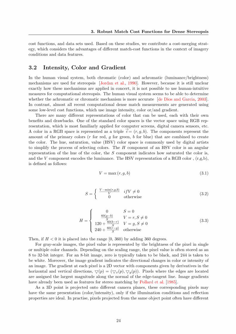
3. Robust Match Cost Functions for Dense Stereopsis
cost functions, and data sets used. Based on these studies, we contribute a cost-merging strat-egy, which considers the advantages of different match-cost functions in the context of imageryconditions and data features.
3.2 Intensity, Color and Gradient
In the human visual system, both chromatic (color) and achromatic (luminance/brightness)mechanisms are used for stereopsis [Jordan et al., 1990]. However, because it is still unclearexactly how these mechanisms are applied in concert, it is not possible to use human-intuitivemeasures for computational stereopsis. The human visual system seems to be able to determinewhether the achromatic or chromatic mechanism is more accurate [de Dios and Garcia, 2003].In contrast, almost all recent computational dense match measurements are generated usingsome low-level cost functions, which use image intensity, color or/and gradient.
There are many different representations of color that can be used, each with their ownbenefits and drawbacks. One of the standard color spaces is the vector space using RGB rep-resentation, which is most familiarly applied for computer screens, digital camera sensors, etc.A color in a RGB space is represented as a triple
→c= (r, g, b). The components represent the
amount of the primary colors (r for red, g for green, b for blue) that are combined to createthe color. The hue, saturation, value (HSV) color space is commonly used by digital artiststo simplify the process of selecting colors. The H component of an HSV color is an angularrepresentation of the hue of the color, the S component indicates how saturated the color is,and the V component encodes the luminance. The HSV representation of a RGB color , (r,g,b),is defined as follows:
V = max (r, g, b) (3.1)
S =
{V−min(r,g,b)
V ifV 6= 00 otherwise
(3.2)
H =
0 S = 0
60(g−b)S V = r, S 6= 0
120 + 60(b−r)S V = g, S 6= 0
240 + 60(r−g)S otherwise
(3.3)
Then, if H < 0 it is placed into the range [0, 360) by adding 360 degrees.For gray-scale images, the pixel value is represented by the brightness of the pixel in single
or multiple color channels. Depending on the scaling range, the pixel value is often stored as an8 to 32-bit integer. For an 8-bit image, zero is typically taken to be black, and 244 is taken tobe white. Moreover, the image gradient indicates the directional changes in color or intensity ofan image. The gradient at each pixel is a 2D vector with components given by derivatives in thehorizontal and vertical directions, 5(p) = (5x(p),5y(p)). Pixels where the edges are locatedare assigned the largest magnitude along the normal of the edge-tangent line. Image gradientshave already been used as features for stereo matching by Pollard et al. [1985].
As a 3D point is projected onto different camera planes, these corresponding pixels mayhave the same presentation (color/intensity), only if the illumination conditions and reflectionproperties are ideal. In practise, pixels projected from the same object point often have different
24

3. Robust Match Cost Functions for Dense Stereopsis
colour/intensity values in two images. Pixel-wise brightness constancy is disrupted by radio-metric changes and noise. With the exception of underexposure or overexposure, color gradientsare, due to significant edge locations, normally less sensitive to radiometric changes. However,match measures using gradient images are limited in homogenous regions, uncertain localizationof features and the gradient-derivation direction1. In homogenous regions, the image gradientsare frequently similar. The gradients can be observed not only on object boundaries, but alsoon surfaces, depending on the image textures. Even edges of object boundaries can be shiftedbetween two input images due to changing view points, especially for stereo pairs with a largebaseline. Moreover, a gradient image is often derived in the x and/or y direction, which causessome lines parallel to these directions having very low gradient values.
3.3 Parametric Match Costs
Parametric match costs are commonly pixel-based and include absolute differences, squared dif-ferences, and the truncated versions using intensities, colors or gradients. The basic assumptionof most parametric cost functions is the brightness/gradient constancy between two correspond-ing pixels.
The simplest cost function is the absolute difference (AD), which can only work on datawith the Lambertian reflectance and good camera configurations. In Equation 3.4, Is(p) andIm(p− δ) denote the intensities of pixel p in the source image and its corresponding pixel withdisparity δ in the match image separately.
CAD(p, δ) = |Is(p)− Im(p− δ)| (3.4)
A user-defined threshold is often used to truncate the maximal intensity difference between twopixels in order to suppress outliers. The truncated absolute difference (TAD) is then defined as:
CTAD(p, δ) =
{T |Is(p)− Im(p− δ)| > T
|Is(p)− Im(p− δ)| otherwise(3.5)
For multi-channels images, the intensity defined in Equation 3.4 and 3.5 can be replaced bycolors or color gradients.
Spatial aggregation is optionally used to limit the influence of mismatches. The basic as-sumption of the spatial aggregation is that the disparities within a small region are almostconstant. Typical spatially aggregated cost functions include the sum of absolute/squared dif-ferences (SAD/SSD) [Kanade, 1994; Matthies et al., 1989] and normalized cross correlation(NCC) [Ryan et al., 1980]. These cost functions measure the compatibilities between source andmatch images with a candidate shift at every pixel. A constant offset (bias) of pixel intensityvalues is compensated by the zero-mean versions ZSAD and ZSSD. Such methods are oftenapplied with winner-takes-all optimization as local stereo algorithms.
The sum of absolute differences (SAD) method is done by summing of intensity/color differ-ences over a rectangle window:
CSAD(p, δ) =1
m× n∑
p∈W,δ∈D|Is(p)− Im(p, δ)| (3.6)
1Generally, the gradients should be derived in the diagonal direction of the epipolar line.
25

3. Robust Match Cost Functions for Dense Stereopsis
Similarly, the normalized cross correlation (NCC) is defined as the product of the two intensityvectors normalized over a window:
CNCC(p, δ) =1
n
∑q∈Np
Is(q)Im(q − δ)√∑q∈Np
Is(q)2∑
q∈NpIm(q − δ)2
(3.7)
where n is the number of pixels in Np.The matching performance of spatial aggregations depends on the window size used, which
is typically fixed. Finding an optimal size for the whole image is impossible. A large windowsize includes enough colour/intensity variations for robust matching on object surfaces, but atthe cost of over-smoothing. Figure 3.1 demonstrates the resulting differences of SAD using var-ious window sizes. Some adaptive-window approaches select the optimal window sizes and/orshapes automatically according to local structures such like color gradients [Boykov et al., 1998;Kanade and Okutomi, 1994b; Veksler, 2003]. Segmentation-based approaches select the aggre-gation shapes using given segments of the input source image [Gong and Yang, 2005b; Tao andSawhney, 2000; Wang et al., 2004]. Such approaches can improve matching performance, only ifthe pre-processing – feature detection or segmentation, works well. Moreover, cost aggregationprefers fronto-parallel surfaces such that all pixels within a support window are assigned thesame disparity.
(a) 3 × 31 (b) 7 × 13 (c) 9 × 31 (d) Reference image
Figure 3.1: WTA results of SAD using various window sizes. Large window size reduces noisesin cost of over-smoothing.
The advantage of cost aggregations with a fixed window size is that the calculation canbe implemented on parallel architecture – for example, modern graphics cards (GPUs). Thecomputation time of cost aggregations using regular window increases proportionally to thewindow size [Zhu et al., 2010]. For instance, Figure 3.2 shows the run-time comparison of SADwith different window sizes on a 480 × 375 pixels stereo pair with 64 pixels disparity range usinga NVIDIA GeForce GTX 295 graphics card.
Wm×n n=3 5 7 9 11 13 15 17 21 25 29
m=3 4.9 8.4 10.0 14.3 18.6 121.0 59.5 67.1 82.2 97.3 113.2
5 9.5 13.8 18.1 24.6 30.1 37.3 122.5 138.4 170.2 201.9 234.6
7 14.6 22.7 29.3 38.3 48.1 59.5 194.6 220.0 270.6 322.0 371.9
9 17.3 26.2 35.9 45.6 56.9 69.7 235.4 266.3 327.7 389.9 451.4
Figure 3.2: The run-time analysis of the SAD method with different fixed window sizes m × nusing CUDA on GPUs.
26

3. Robust Match Cost Functions for Dense Stereopsis
3.4 Mutual Information
Mutual information (MI) is introduced by Shannon [1948] and popularized for image registrationproblems by Viola and Wells [1997]. It is used to measure the similarity between images and isrealized by some variant of gradient descent [Kim et al., 2003; Viola and Wells, 1997]. Egnal[2000] has introduced applying mutual information for correlation based dense stereo matching.The key advantage of mutual information is the ability of handling complex radiometric rela-tionships between intensities of images. In stereopsis, mutual information can be insensitive torecording and illumination changes [Hirschmuller and Scharstein, 2009]. In order to obtain areliable initial disparity map, Hirschmuller [2008] presents a hierarchical strategy to calculatejoint entropy iteratively and efficiently.
Give a stereo pair Is, Im and an initial disparity map ∆, let I ′m = ∆(Im) be the warpedimage according to ∆. The mutual information is defined by the individual entropies of inputimages and their joint entropy, HIs,I′m
:
MIIs,I′m= HIs +HI′m
−HIs,I′m (3.8)
where the entropies are calculated by the probability distribution of intensities from Is andassociated I ′m:
HI = −∫ 1
0PI(i) logPI(i)di (3.9)
HIs,I′m= −
∫ 1
0
∫ 1
0PIs,I′m
(is, im) logPIs,I′m(is, im)disdim (3.10)
with I ∈ {Is, I′m} and i ∈ [0, 255]. This definition of mutual information is over the full
images and requires the disparity map a priori to calculate the joint entropy. To allow pixel-wisematching, Kim et al. [2003] introduce a transformation of 3.10 into a sum over overlapping pixelsusing Taylor expansion:
HIs,I′m=∑p
hIs,I′m(Is(p), I
′m(p)) (3.11)
where hIs,I′mis calculated by the joint probability distribution PIs,I′m
of corresponding intensi-
ties. Under the assumption of the individual entropies are almost constant, Kim et al. [2003]define the data energy of 2.15 as the negative sum of hIs,I′m
(mutual information is maximized,
while energy is minimized). However, the intensities having non-correspondence in occlusionareas should not be included in the calculation [Hirschmuller, 2008]. They suggest to considerthe individual entropies in data term to improve object borders:
HI =∑p
hI(I(p)) (3.12)
Finally, given a disparity map ∆, we can quantify 3.8 by the pixel-wise summing over thewhole image:
MIIs,Im,∆ = −Edata = −∑p
CMI(p, δ) (3.13)
where δ = ∆(p). The matching cost function using mutual information is now defined as:
CMI(p, δ) = −hIm(Im(p))− h∆(Is)(Is(p, δ)) + hIm,∆(Is)(Im(p), Is(p, δ)). (3.14)
27

3. Robust Match Cost Functions for Dense Stereopsis
3.5 Non-Parametric Matching Costs
Zabih and Woodfill [1994] introduce non-parametric local transforms for computing optical cor-respondences. Their approach includes two local transforms, rank and census, which rely onthe relative order of local intensity values, not the values themselves. Since all non-parametriccost functions calculate the match distance only depending on the ordering of colours/intensitiesand not the magnitude of intensities, they tolerate all radiometric distortions that preserve thisordering.
The implementations of rank and census transformation are filtering followed by a comparisonusing the absolute difference or Hamming distance. Permutations of two corresponding windowsare ranked and their alignment bits are calculated to measure the feature distance. Ranktransform of an image, I, is defined as the amount of pixels within a local region, whose intensityis lower than the center pixel.
RankI(p, q) = ‖{q ∈ Np|I(q) < I(p)}‖ (3.15)
The rank transformation is known to be susceptible to noise in textureless areas. Thus, wedefine the match cost using the rank transformations of Is and Im as follows:
CRank(p, p′) = |RankIs(p, q)−RankIm(p′, q′)| (3.16)
where p′ ∈ Im is the wrapped pixel of p ∈ Is with p′ = p− δ.Census transformation is invariant to monotonic gray value changes, and thus, can tolerate a
large class of global and local radiometric changes. It encodes the local image structure within atransform window and defines a bit string where each bit describes the relative ordering betweenthe computing pixel and its local neighbor. A bit is set if a pixel inside the window has a lowerintensity than the center pixel. The distance between two bit strings is computed using theHamming distance. In our work, a 9 × 7 1 window is used and supports the matching costs inthe range of 0 to 63 2. ξ denotes a census transform within a window of image I, W (I).
⊗computes the Hamming distance:
CCen(p, δ) =⊗
( ξW (Is)
(p), ξW (Im)
(p− δ)) (3.17)
Figure 3.3 illustrates the calculation of a census match cost using a 3×3 window. Each pixelwithin this window is compared with the center pixel such that a binary bits code is built todescribe the local structure. Doing bitwise exclusive or of two bit strings and summing all bitsequal one, the local difference between two windows is calculated.
In contrast to parametric match costs and spatial cost aggregations, non-parametric matchcosts such as census transformation have advantages in the following ways:
• encoding local spatial structure, which is relative insensitive to radiometric changes;
• reducing effects of variations caused by the camera’s gain and bias;
• increasing robustness in dealing with outliers near to depth-discontinuities; and
• tolerating to factionalism. If a minority of pixels in a local neighborhood has a highlydifferent intensity distribution than the majority, only comparisons involving a member ofthe minority are affected.
1Small window size reduces the matching robustness. Large window size leads to blurring.264 bits is the maximal bit size allows a fast implementation.
28

3. Robust Match Cost Functions for Dense Stereopsis
27 45 47 0 1 1 0 1 1 0 127 45 47
29 30 43
31 28 45
0 1 1 0 1 1 0 1
0 0 0 0 0 1 0 0XORW(Is)
43>30?0:13 8 45
31 47 50
30 32 46
0 1 1 0 1 0 0 1∑(bit==1) = 1
W(I )
43>30?0:1
30 32 46
31 29 47
W(Im)
31>32?0:1
Figure 3.3: Illustration of calculating census match cost.
However, compared with parametric match costs and mutual information, non-parametricmatch costs have loss of information associated with the pixel due to the window-based compu-tation. Local transformations using large window sizes lead to dilated object edges. To avoidblurring and for a fast implementation, we used to use a window size with maximal 7× 9 pixels.The magnitude of intensities is therefore strongly elided in contrast to gray values. For a censuswindow of 3× 3 pixels, the variable to store the census value would be of size 23, or 8 bits; fora census of window size 5× 5 the number of bits required to store the census value would be 25bits.
3.6 Match costs merging
Same match cost can perform differently with respect to regions used, even within a same stereopair. Our motivation of merging match costs comes from such context-dependent performancesof match costs. Most stereo methods have been developed using in-lab captured stereo pairs.How far can such data differ from real-world data? Figure 3.4 (c) and (d) demonstrate theradiometric changes of a Middlebury stereo pair and an airborne stereo pair with large baselinerespectively. The lightness densities of the Flowerpots stereo pair in HSV color space are highlysimilar, thus parametric costs are able to measure similarity of corresponding pixels. In contrast,the lightness distributions on building roofs of the airborne stereo pair are quite different.
Various cost functions perform differently in context of illuminations, object type (land-scapes), and stereo configurations. In fact, all factors appear concurrently such that a separateevaluation for each factor is impossible. In Table 3.1, based on the evaluation shown in Chapter5, we summarize the performances of match costs in scale according to four criteria: how largeare the radiometric changes between two stereo images; how lange is the baseline between twocamera principle points; how rich is the image textured?; and how smooth is the scenario? Inthe first row of this table, the light colors of gray bars indicate less radiometric changes, shortbase line, less texture, and less smoothness of the object respectively, vise versa. Matchingperformances under these criteria are scaled from light (for bad match) to dark (for good androbust match) colors. For instance, non-parametric cost functions perform more robust thanmutual information in weekly-textured regions. But, mutual information can generate sharperedges than non-parametric costs. As shown in this table, different match cost functions are com-plementary in different situations. Thus, match-costs merging according to imagery conditionscan combine their advantages and improve matching performance in robustness and accuracy.
In this work we merge absolute difference (AD) or mutual information (MI) with censusrespectively using a weighted average::
Cx+Cen(p, δ) = wx×Cx(p, δ) + (1− wx)×CCen(p, δ). (3.18)
29

3. Robust Match Cost Functions for Dense Stereopsis
(a) Flowerpots from Middlebury stereo pairs and mask on pots surfaces
(b) Airborne stereo pair with large baseline and mask on building roofs
Source Image
Match Image
Lightness
Den
sity
-20 20 60 100 140 180
0.025
0.02
0.015
0.01
0.005
(c) Lightness density of (a)
Lightness
Den
sity
0 50 100 150 200 250 300
0.015
0.01
0.005
(d) Lightness density of (b)
Figure 3.4: Lightness densities of two stereo pairs in HSV colour space. The analyses are limitedusing the masks for object surfaces and building roofs respectively. The images of Flowerpotshave similar lightness distributions shown in (c). In contrast, the lightness densities of twoairborne images are different as shown in (d).
where x is either absolute difference or mutual information. For easier combination with othercosts, we rescale each match cost into a range from 0 to 1023. wx denotes the weight parameter,which is scaled in the range [0, 1].
The most important reasons for radiometric changes in a real-world application are dynamiclight sources and large stereo baseline. In the case of stereo pairs with static light sources andsmall baseline, the radiometric changes for corresponding pixels are comparatively less presented.
30

3. Robust Match Cost Functions for Dense Stereopsis
Data with Radiometric Changes Baseline Length Texture Smoothing
- + - + - + - +
Parametric Costs + - - + - - - + + -
Mutual Information + - + - - - + + -
Non-parametric Costs + - + - - + - +
Table 3.1: A qualitative comparison of match costs under different criteria. The light color in agray bar in the first row indicates less radiometric changes, short base line, texture-less regionsand less smoothing on result, vise versa. Matching performance is scaled from light (for bed)and deep (for good) colors.
Non-parametric match costs perform more robust than other cost functions for data sets withlarge radiometric changes and homogenous surface areas. However, parametric match costsand mutual information generate sharp edges, if the photogrammetric consistencies remain in astereo pair. Thus, the weight parameter wx should be adapted to imagery conditions in orderto use the advantages of different match costs. In chapter 5, we demonstrate the parametertuning of wx for stereo pairs with a increasing baseline length and show the dependence betweenmatching performance and the weight selection.
Matching cost intensity-based gradient-based
Absolute Difference CAD(I3→1) CAD(5eI)Mutual Information CMI(I3→1) CMI(5eI)
Census CCen(I3→1) CCen(5eI)Sum of AD and Cen CAD+Cen(I3→1) CAD+Cen(5eI)Sum of MI and Cen CMI+Cen(I3→1) CMI+Cen(5eI)
Table 3.2: Abbreviations of different match costs. We consider both gray value and gradientbased variants of matching costs. Color channels are averaged, if they are available. The gradientimages are created using the partial derivative with respect to the epipolar direction.
3.7 Summary
Match cost is one of the most important components of stereo processing. All stereopsis algo-rithms need match costs to measure the similarity of two corresponding pixels or regions. Therobustness of a match cost is decisive for the matching performance, also for global methods.
In this chapter we describe parametric, non-parametric match costs, and the match costbased on mutual information. We analyzed their advantages and disadvantages from theirmathematical definitions. Their matching performances are qualitatively summarized in contextof data (radiometric changes, object features) and observation conditions (stereo baselines).Depending on applications, all these challenges might be present at the same time. Thereis no single cost function that performs best for all circumstances. Parametric match costswithout spatial aggregations are pixel-wisely calculated, thus fine details, such as building edges,can be accurately reconstructed. Match costs based on mutual information expose the globalradiometric relationship between two images and can reduce effects of variations caused by thecamera’s bias and gains. Non-parametric match costs encode image local structures and areinvariant to any monotonic radiometric changes. However the window-based mechanisms ofnon-parametric costs cause lose of shape edges and fine details. To develop match costs for
31

3. Robust Match Cost Functions for Dense Stereopsis
real-world data, we introduce the cost-merging strategy with respect to the imagery contextslike stereo baseline length.
In this dissertation absolute difference, mutual information, and census are evaluated usingintensity as well as gradient images. In addition, the linearly merged match costs using ADand MI with census respectively, are compared with the conventional match costs. Table 3.2summarizes the abbreviations of all ten match costs used in this work. For a representativeevaluation, both the Middlebury data sets with/without radiometric changes and the remote-sensing data with short/long baselines are used in Chapter 5.
32

Chapter 4
Probabilistic Pixel-wise SurfaceStereo
In this chapter we introduce a probabilistic model for pixel-wise surface stereo matching. Thisapproach builds a surface prior over the disparity space using the confidence based on a setof reliably matched correspondences. For each pixel, the probability of its depth lying on anobject plane is modeled as a Gaussian distribution, whose variance is determined using theconfidence from a previous matching. We minimize our global formulation in energy space usingiSGM3 – a modified semi-global optimization for three terms. This method is iterative. Sincethe confidences are derived with respect to image likelihood and smooth prior probability, ourapproach has decreased sensitivity to a given image segmentation in comparison to existingsegment-based stereo methods.
Global energy minimization algorithms that are defined over image regions, rather thanpixels, achieve the top few ranks in the de-facto standard Middlebury online benchmark whensorted according to depth discontinuities (disc) [Bleyer et al., 2010, 2011; Klaus et al., 2006;Scharstein and Szeliski, 2002; Taguchi et al., 2008; Wang and Zheng, 2008]. Our own experienceand the Middlebury benchmark indicate that these region-based methods are preferable aroundobject boundaries and in large homogeneous areas; the use of regions helps propagate strongmatches into sub-regions with poor matches. However, defining an energy minimization overregions, rather than pixels, imposes a hard constraint that forces depths to lie on the smoothsurface associated with a region; removing fine-level details from the depth map in the process.In our method, we relax the hard region-surface constraint imposed by these methods andcontinue to gain the benefits of region-based methods by defining an energy minimization overpixels that incorporates a probabilistic constraint that depths lie near, rather than on, a pre-calculated smooth surface. We adjust the strength of our constraint using a measure of theconfidence we have that the smooth surface is correct; relaxing the constraint when we believethat it will not benefit the disparity calculation.
As shown in Figure 4.1, the introduced confidence-based surface prior for global energyminimization formulation addresses these problems:
• Foreground/background fattening : Often observed in the occlusion areas of Middleburybenchmark sets Scharstein and Szeliski [2002] and in the shadow regions of remote sensingdata Kurz et al. [2012], objects are dilated into weakly matching areas. This problemis demonstrated in Figure 4.1: the pink teddy bear, church towers, and the edges ofbuildings that are near shadowed streets. The matching costs are ambiguous, causing theenergy minimization to dilate the objects beyond their borders. Robust matching cost like
33

4. Probabilistic Pixel-wise Surface Stereo
(a) Source images (b) Results using SGM (c) Segmentation of (a) (d) Results using hard constraint
Figure 4.1: Segment-based stereo matching is very sensitive to the given segmentation. Asthis hard plane constraint performs well on Teddy (less blurring within the white maskers),segmentation artifacts are observed on the texture-rich areas of Cloth3. The result of theairborne image including a large homogenous roof has generally sharper building shapes usingthe hard constraint. However, a lot of shadowing streets are enforced as a disparity-plane partof the building roofs.
Mutual Information Viola and Wells [1997] can improve the matching performance onlypartially Hirschmuller and Scharstein [2009]; Zhu et al. [2011].
• Sensitivity to image segmentation: As shown in Figure 4.1, segmentation-based meth-ods can perform very well, if the given segments are correlated with the object bound-aries Bleyer et al. [2010]; Klaus et al. [2006]; Taguchi et al. [2008]; Wang and Zheng [2008].However, the results are very sensitive to the given segmentations. Oft over-segmentationis required. In texture-rich regions, artifacts from segmentation can be appeared.
• Incorrect matching in large homogeneous areas: In a large low-texture or homogeneousarea, parametric match costs can be unreliable; even when using a global energy minimiza-tion algorithm. This is demonstrated in the church roof in Figure 4.1. Non-parametric,window-based, matching costs like census Zabih and Woodfill [1994] can overcome thisproblem, but can lead to dilated edges Zhu et al. [2011].
In this chapter, the formulation and the implementation of the proposed probabilistic surfacestereo method are introduced. The performance of this approach using both the Middleburybenchmark data sets and the real-world remote sensing data is discussed in Chapter 5. The
34

4. Probabilistic Pixel-wise Surface Stereo
remainder of this chapter is organized as follows. In Section 4.1 the related works are outlined.Section 4.2 introduces the hard surface constraint used for stereo matching and points outits limitations. Then, we describe the confidence-based surface prior for energy optimizationin Section 4.3. Finally, the iSGM3 optimization for an energy formulation with data term,smoothness prior, and surface constraint is introduced in Section 4.4.
4.1 Related Work
One of the main defects of pixel-wise matching is the absence of semantic information. Pixel-wise observation is limited within a small and often a regular window, even using some adaptivestrategy. Image features like edges, corners and line segments are sparse and heterogeneouslydistributed. Combining such feature primitives with dense matching methods is prevented intexture-less regions such like occlusions and shadow regions, because the data costs are ambigu-ous. In contrast, color segment allows to trade similar pixels as a whole unit. In this section,we throw a brief overview about the methods developed in the last years.
The works of Koschan et al. [1996]; Wei and Quan [2004] assume that pixels within a seg-ment have the same disparity. Over-segmentation and region splitting are required to relax theconstraint. Tao and Sawhney [2000] enforce the depth of each homogeneous region as a nominalplane with allowable additional smooth depth variations. Cai et al. [2005] employ matchingsegments on scanlines using fuzzy set theory to handle ambiguities.
More relevant to this dissertation are methods formulated as a global energy function. Manyof the best ranked methods in the Middlebury online benchmark use a region-based, ratherthan pixel-based, global approach [Klaus et al., 2006; Taguchi et al., 2008; Wang and Zheng,2008]. These approaches define Equation 2.15 in a way that assigns a smooth surface (usually aplane) to image regions, rather than depth to pixels. The performance of this hard constraint,that all depths in a region be on the same smooth surface, is highly influenced by the qualityof the subdivision of the image into regions. If depth discontinuities are not coincident withthe border between regions, then they will be lost in the resulting disparity map. Thus, thesemethods rely on over-segmentation of the image into small regions to maintain good accuracy.By incorporating a soft, rather than a hard, constraint the proposed method is very robustto the color segmentation of the image into regions. Saygili [2012] initiate a disparity map bymatching with SURF key points. Each image segment is assigned with a disparity plane usinggraph cuts. Aydin and Akgul [2010] introduces a synchronous energy optimization with segmentbased regularization.
Sun et al. [2005], Bleyer et al. [2010], and Woodford et al. [2009] have all proposeddifferent soft constraints for region-based stereo algorithms that are different from our proposedconstraint. The soft constraint proposed by Sun et al. is most similar to the proposed methodin that they introduce the addition of a single soft constraint term to the energy minimizationformulation in Equation 2.15 that encourages the disparity of a pixel to lie near a plane calculatedfrom a given disparity estimation. However, their soft region constraint does not incorporateconfidence; they assume that the provided disparity estimation is trustworthy. The algorithmsproposed by Bleyer et al. [2010, 2011] split a given segmentation into overlapping subsegments,and add a term to their formulation that softly constrains overlapping segments to contain asingle contiguous surface. Their energy formulations with seven optimization terms could leadto parochial usability depending on applied scenes. Unlike the proposed method, Woodford etal. utilize an over-segmentation of the image into many small regions, and propose a weightingof their smoothness term that discourages disparity edges from cutting through regions.
Common methods for deriving an approximate minimum of Equation 2.15 include loopy
35

4. Probabilistic Pixel-wise Surface Stereo
belief propagation [Pearl, 1988; Sun et al., 2003], graph cuts [Boykov and Kolmogorov, 2004],iterated condition modes [Jodoin and Mignotte, 2004], fusion moves [Lempitsky et al., 2007], anddynamic programming [Gong and Yang, 2003; Hirschmuller, 2008]. The semi-global matchingmethod proposed by Hirschmuller [Hirschmuller, 2008] is widely used in the photogrammetry,remote sensing, and intelligent vehicle application areas due to being orders of magnitude fasterthan the other methods of optimization while still producing high quality results.
4.2 Hard Surface Constraints
Several factors drive us to add surface prior into global energy formulations, softly. A globalmethod enforces smoothness of results by minimizing a MRF-based energy function, whichtypically can be decomposed into two parts, an image likelihood and a smoothing prior. Oftenthe smoothness assumption has to be compromised with the match costs in order to allowsharp edges in large discontinuity areas. However, a suitable smoothing degree is difficult to befound. Choosing a large smoothing strength leads to over-smoothing and foreground fattening.In contrast, less smoothing can result in noise on object surfaces. Adapting smoothing penaltyaccording to edge locations relies strongly on edge extraction [Banz et al., 2012; Gong and Yang,2005a]. Moreover, stereo methods without surface prior favor fronto-parallel planes instead ofslanted surfaces.
Object-surface prior can potentially contribute energy optimization for slanted surfaces byremaining discontinuity of object boundaries. But object surfaces are unknown. What we canobtain directly from input images are segments based on color/intesity similarity. Segments arelimited in the 2D image domain and their boundaries can differ from the real object separation.Moreover, the segmentations of source and matching images are often not the same. In orderto obtain object surfaces, pixel-wise disparities are fitted to segments such that many disparityplanes are calculated. However, the main limitation of fitting planes is its high sensitivity to thesegmentation initialization.
Figure 4.2 shows both positive and negative influences of initial subdivision by fitting dis-parity planes. Once a segment includes pixels only within an object surface, a plane-fit regioncan be reconstructed smoothly with sharp edges in discontinuity area (see the triangular build-ing boundary). If segment contains pixels belonging to different object surfaces, any hardconstrained region is completely failed (roof windows segmented with building facades). Meth-ods [Klaus et al., 2006; Saygili, 2012; Taguchi et al., 2008; Wang and Zheng, 2008] employ en-ergy minimization in a surface space as shown in Equation 2.16 are able to correct mis-matchesonce the color segmentation is wrong. Thus, almost all existing segment-based stereo match-ing methods require over-segmentation, which leads to very small segments. This limitation iscontradictory to obtain reliable disparities within a segment for a robust plane fitting.
4.3 Confidence-Based Surface Prior
We calculate a disparity map ∆ for Is and denote the probability of ∆(p) = δp being correctas P(δp) where P(δp) = max{P(δ) : ∀δ}. Then we segment Is into contiguous regions usingthe well-known mean-shift segmentation algorithm Comaniciu and Meer [2002] 1. Using thedisparity map ∆ and the segmentation Segs, we fit a slanted plane, in disparity space, to eachregion in the segmentation. The plane fitting results in a dense disparity plane map for Is thatwe will denote ∆pl : Is → Z>0. Each pixel p ∈ Segms has to belong to a disparity plane Πm with
1Note that we do not require that this segmentation be an over-segmentation.
36

4. Probabilistic Pixel-wise Surface Stereo
(a) Reference images. (b) Segmentation of (a). (c) Plane-fit disparity maps from(b).
Figure 4.2: Problem statement of using hard surface constraint. Mis-matches are indicated bysolid black regions using consistence checking. Top: As the building roofs are clearly separatedwith the streets, hard surface constrain reconstructs sharp edges on object boundaries. Bottom:Roofs, building facades and part of streets in (a) are partitioned within a same segment in (b).Using hard constraint leads to failed matching shown as solid black regions in (c)
m ∈ [0, ..., |Segs|). The disparity of pixel p after plane fitting is denoted as dp, which can differfrom δp calculated from the initial pixel based matching process.
The plane fitting provides a unique assignment for each pixel. The goal of our work is to usethis result as an additional surface prior for global frameworks in a probabilistic way. Thus weassume:
Assumption 4.3.1. ∀p ∈ Is: P(∆pl(p)) ∼ N(µ = dp, σ2)
Assumption 4.3.2. P(∆(p) = dp) � P(∆(p) = δp) ⇒ ∆(p) 6∈ Πm
Assumption 4.3.1 indicates that the probability of ∆pl(p) is normally distributed at mean µ = dpcalculated by plane fitting. Assuming a normal distribution allows us to take advantage of itsproperties and make inferences from a hard planar constraint to a probabilistic surface prior.Assumption 4.3.2 builds the probability of ∆(p) ∈ Πm according to a confidence observed fromthe initial pixel based matching. The confidence is obtained by comparison of P(δp) and P(dp).The standard deviation is then defined as:
σ = t(P(dp),P(δp)) (4.1)
where t is a function such that σ2 ∝ log(P(δp)/P(dp)). Recall that a high value for P(dp)indicates that dp is a good candidate match for p. Thus, since σ2 is the variance, it will causea sharply peaked Gaussian distribution with its maximum at µ = dp when we are confident
37
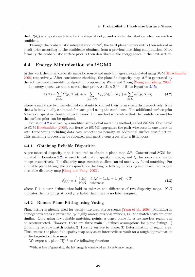
4. Probabilistic Pixel-wise Surface Stereo
that P(dp) is a good candidate for the disparity of p, and a wider distribution when we are lessconfident.
Through the probabilistic interpretation of ∆pl, the hard planar constraint is then relaxed asa soft prior according to the confidence obtained from a previous matching computation. Moreformally the probabilistic surface prior is then described in the energy space in the next section.
4.4 Energy Minimization via iSGM3
In this work the initial disparity maps for source and match images are calculated using SGM [Hirschmuller,2008] respectively. After consistence checking, the plane-fit disparity map ∆pl is generated bythe voting-based plane-fitting algorithm proposed by Wang and Zheng [Wang and Zheng, 2008].
In energy space, we add a new surface prior, S : Is × Z>0 → R, to Equation 2.15:
E(∆) =∑p∈Is
C(p,∆(p)) + λ∑
{p,q}∈N
Vp,q(∆(p),∆(q)) +∑p∈Is
κS(p,∆(p)) (4.2)
where λ and κ are two user-defined constants to control their term strengths, respectively. Notethat κ is individually estimated for each pixel using the confidence. The additional surface priorS favors disparities close to object planes. Our method is iterative that the confidence used forthe surface prior can be updated.
Equation 4.2 is solved by a modified semi-global matching method, called iSGM3. Comparedto SGM Hirschmuller [2008], our iterative iSGM3 aggregates the path-wise costs in one directionwith three terms including data cost, smoothness penalty an additional surface cost function.This matching process can be repeated and mostly converges after a little loops.
4.4.1 Obtaining Reliable Disparities
A pre-matched disparity map is required to obtain a plane map ∆pl. Conventional SGM for-mulated in Equation 2.21 is used to calculate disparity maps, δs and δm for source and matchimages respectively. The disparity maps contain outliers caused mostly by failed matching. Fora reliable plane fitting, the correspondence checking or left-right checking is oft executed to gaina reliable disparity map [Gong and Yang, 2003].
δ′s(p) =
{δs(p) |δs(p)− δm(p+ δs(p))| < TNaN otherwise
(4.3)
where T is a user defined threshold to tolerate the difference of two disparity maps. NaNindicates the matching at pixel p is failed that there is no label assigned.
4.4.2 Robust Plane Fitting using Voting
Plane fitting is already used for weakly-textured stereo scenes [Yang et al., 2008]. Matching inhomogenous areas is prevented by highly ambiguous observations, i.e. the match costs are quitesimilar. Only using few reliable matching points, a dense plane for a texture-less region canbe reconstructed. However, there are three main ill-defined assumptions for plane fitting: 1)Obtaining reliable match points; 2) Forcing surface to plane; 3) Determination of region area.Thus, we use the plane-fit disparity map only as an intermediate result for a rough approximationof the targeted surface map.
We express a plane Πmi
1 as the following function:
1Without loss of generality, the left image is considered as the reference image.
38

4. Probabilistic Pixel-wise Surface Stereo
δi(x, y) = a · x+ b · y + c (4.4)
where i ∈ (L,R). (x, y) denotes the image coordinates of pixel p. δi(x, y) is the disparity ofp. We assume each Πm
i contains Nmi reliable match pixels within a segment. Three plane
parameters, a, b and c, need to be estimated.We fit disparity maps in space according to segments. The plane parameters can be solved
though Singular Value Decomposition [Shi and Tomasi, 1994]. Using the reliability of eachdisparity as weight, the normal vector of a disparity plane is given by the eigenvector belongingthe minimum eigenvalue of matrix A.
A =
∑N
t=1wt · x2t
∑Nt=1wt · xt · yt
∑Nt=1wt · xt · δt∑N
t=1wt · xt · yt∑N
t=1wt · y2t
∑Nt=1wt · yt · δt∑N
t=1wt · xt · δt∑N
t=1wt · yt · δi∑N
t=1wt · δ2t
(4.5)
For robust plane fitting, reliable depthes in disparity map are required. However consistencechecking1 eliminates outliers mainly in occlusion areas, mis-matches are not avoidable. Usingthe RANSAC method can remove outliers [Yang and Forstner, 2010], but the results rely on therandomly selected initial points. The comparison of Wang and Zheng [2008] shows the voting-based plane-fitting algorithm is more competent as the RANSAC method for fitting disparitymaps.
Given a disparity map for Ii and the segmentation Segi, we fit a slanted plane, in disparityspace, to each surface in the segmentation using the voting-based plane-fitting algorithm asoutlined in Figure 4.4: The slant of a plane in x direction is obtained by calculation gradients,∂δi∂x , of all possible pixel pairs having the same x, row by row through a segment as shown inFigure. The calculated gradients are voted in a one-dimensional histogram, whose x-coordinatedenotes all options of a and y-coordinate is the count amount of each option. A gaussian filteris executed to smooth the histogram to eliminate outliers, especially at ∂δi
∂x = 0. The maximumof the histogram is regarded as the final estimation of a. Similarly, b can be estimated bycalculating ∂δi
∂y . Once a and b are obtained, according to Equation 4.4, we can estimate c in thesame way using the given disparities δi(p).
x
δ ∂δ/∂x=8/7
1 8
4
8 Πi
6
Segi
4 4 4 4 5 5 5 8 5
x
y
…
1 8
Figure 4.3: Illustration of calculating local gradients for plane fitting within a segment row. Redline denotes a cross-section of plane Πi to be fitted. Local gradients are calculated using allpossible reliable disparity pairs within the same row.
1Or Left-right checking eliminates outliers by comparison the disparity maps from left-right matching andright-left matching.
39

4. Probabilistic Pixel-wise Surface Stereo
1: procedure RegionBasedPlaneFitting( Segi, δi )2: repeat3: ({ ∂δ∂x}, {
∂δ∂y})← GradientCalculation(Segmi , δi)
4: (hx, hy)← HistogramVoting ({ ∂δ∂x}, {∂δ∂y})
5: (h′x, h
′y)← GaussianSmoothing (hx, hy)
6: (a,b)← ParameterEstimation (h′x, h
′y)
7: hc ← HistogramVoting (a, b, δ′i) . Eq. 4.4
8: h′c ← GaussianSmoothing (hc)
9: c← ParameterEstimation (h′c)
10: until M segments completed11: return {Pi}12: end procedure
Figure 4.4: Process of region-based plane fitting using voting. Given a color segment and thedisparity within it, Segi, δi, the proposed method estimates the horizontal and vertical slants,(a, b), of a spatial plane using histograms.
4.4.3 Iterative SGM3
Typical SGM minimization [Hirschmuller, 2008] is operated with a data term and a smoothingterm. It approximates a global, 3D smoothness constraint by combining many 1D constraintsfrom different aggregation directions for pixel-wise matching. To solve Equation 4.2, we intro-duce a modified semi-global matching method, called iSGM3. Compared to SGM [Hirschmuller,2008], our iterative iSGM3 aggregates the path-wise costs in direction r with three terms in-cluding data cost, smoothness penalty and the additional surface cost function S(p, δ) as:
Lr(p, δ) = C(p, δ) + Vp,p−r(δ, δ′) + S(p, δ). (4.6)
where Vp,q is a truncated linear smoothing term with Vp,q(δ, δ′) = min{|δ − δ′|, τ}. δ′ denotes
the disparity at q. The aggregated match costs in different directions, Lr with r ∈ [0, 15], arethen summed in Ei(p, δ):
Ei(p, δ) =∑r
Lr(p, δ) (4.7)
where i denotes the energy calculated at the i-th step. The initial energy at i = 0 can becalculated by Equation 2.15.
According to assumption 4.3.1, we denote the function f(δ) = N(δ, σ(δ)). Using the confi-dence introduced in Equation 4.1, we define σ in the energy space as:
σ(δ) = (Ei−1(p, δ)− Ei−1(p, δp) + ε)2 (4.8)
where ε is a user-defined parameter to avoid a sharply peaked penalty. In the implementation,ε is chosen to be equal to 1.5. A quadratic function is selected over the confidence to smooththe penalties if Ei−1(p, dp) is very close to Ei−1(p, δp). The surface cost function is then definedas follows:
S(p, δ) = (f(dp)− f(δ)) · Ei−1(p, δp)
f(dp)(4.9)
40

4. Probabilistic Pixel-wise Surface Stereo
S(p, δ) penalizes the cost of a pixel belonging to an estimated plane according to its confidence.Choosing δp = arg minδ{Ei−1(p, δ) : ∀δ} causes the strength of our surface constraint similar tothe data cost and smoothness penalty. Therefore, the further the variable δ is away from dp,the higher cost will be penalized. The ratio of the penalty of δ at different disparity levels isdecided by the shape of f(δ), whose σ is derived from the confidence.
Figure 4.5 demonstrates the influence of the confidence by fusing the previous calculatedEi−1(p, δ) and the surface penalty, S(p, δ). We define δ′p as the new calculated disparity at pixelp for the step i with δ′p = arg minδ′{Ei(p, δ′) : ∀δ′}. A small difference between Ei−1(p, δp) andEi−1(p, dp) indicates a good confidence for disparity of p lying on the plane shifting δ′p near todp. Conversely, a bad confidence causes a small penalty that δ′p remains at the same position asthe previous result.
E i−1( p ,δ)S ( p ,δ)E i( p ,δ)
Confidence
Cost
d p δ p
(a)
E i−1( p ,δ)S ( p ,δ)E i( p ,δ)
Confidence
Cost
δ pd p(b)
Figure 4.5: Cost fusion using surface prior: The green line denotes the previously computedcosts for one within a disparity range. The blue line is the surface penalty S from the planefitting processing. The fused cost is shown as the red line. (a) Good confidence: The disparityis shifted near to the plane-fit result. (b) Bad confidence: Surface penalties are overall similar.The disparity remains at the early position.
The proposed algorithm to employ the confidence-based surface prior is outlined in Fig-ure 4.6. This algorithm employs an iterative feedback loop to incrementally improve the pro-duced disparity estimates; in practice we observe convergence of the depth estimation in one tothree iterations. For instance, we demonstrate our method in Figure 4.7: We fit the disparitymap of (d) in space according to segments in (b). The plane-fit result is shown in (e) withobservable effects of segments. The final disparity map is calculated in (f).
4.5 Summary
In this chapter the confidence-based surface prior for global energy minimization formulationsis introduced. Given a dense disparity estimation we fit planes, in disparity space, to imagesegments. For each pixel, the probability of the depth of a pixel lying on an object plane ismodeled as a Gaussian distribution, whose variance is determined using the confidence from aprevious matching. A new disparity estimation with the addition of our confidence-based sur-face prior is than recalculated. This process can be then repeated. The confidence-based surfaceprior differs from existing surface constraints in that it varies the per-pixel strength of the con-straint to be proportional to the confidence in our given disparity estimation. The global energy
41

4. Probabilistic Pixel-wise Surface Stereo
1: procedure CalcDisparity( IL, IR )2: SegL ← Segmentation(IL)3: SegR ← Segmentation(IR)4: CL, CR ← CalculateMatchCosts(IL, IR)5: (∆L,E
′L)← SGM(CL, IL as Is) . Eq. 2.15
6: (∆R,E′R)← SGM(CR, IR as Is) . Eq. 2.15
7: repeat8: ∆
′L,∆
′R ← LeftRightConsistency(∆L,∆R)
9: ∆plL ← RegionBasedPlaneFitting(SegL,∆
′L)
10: ∆plR ← RegionBasedPlaneFitting(SegR,∆
′R)
11: SL ← CalculateConfidenceConstraint(∆plL ,E
′L)
12: SR ← CalculateConfidenceConstraint(∆plR ,E
′R)
13: (∆L,E′L)← iSGM3(CL + SL, IL as Is) . Eq. 4.2
14: (∆R,E′R)← iSGM3(CR + SR, IR as Is) . Eq. 4.2
15: until N iterations completed16: ∆
′L,∆
′R ← LeftRightConsistency(∆L,∆R)
17: return {∆′L,∆′R}
18: end procedure
Figure 4.6: Proposed iterative algorithm. Given a stereo image pair, {IL, IR}, the introducedmethod calculates an initial disparity map. The resulted match costs are used as the confidenceof the plane-fit process. iSGM3 aggregates the previous match costs and generate iterativelydisparity maps.
minimization with three priors – the data, smoothness and surface prior, is computationallysolved by the algorithm – iterative Semi-Global Matching with 3 terms (iSGM3), which inher-its the (efficient) path-wise cost aggregation from SGM and adds the confidence-based surfaceprior into the framework. Unlike many region-based methods, the iSGM3 method defines theenergy formulation over pixels, instead of regions in a segmentation; this results in a decreasedsensitivity to the quality of the initial segmentation, especially in texture-rich regions, where anobject surface is oft over-segmented. In contrast, iSGM3 trends to handle homogenous regionsas an integral part, where pixel-wise matching costs are very similar. Generally the introducedmethod has three main benefits for solving dense stereopsis: sharp object-boundary edges inareas of depth discontinuity; accurate disparity in surface regions; and low sensitivity to theinitial color segmentation.
42

4. Probabilistic Pixel-wise Surface Stereo
(a) Reference image (b) Ground truth. (c) Segmentation of (a)
(d) SGM result (e) Plane-fit disparity map of (d) (f) iSGM3 result
Figure 4.7: Illustration of processing steps of iSGM3: Initial disparity map (d) is fitted tosegments of (c) in order to compute a plane map (e). The pixel-wise confidence is generated bycomparing energies at disparity levels (d) and (e). (f) is the result using iSGM3.
43

Chapter 5
Results
As introduced in Scharstein and Szeliski [2002] the performance of a global dense stereo match-ing method depends on several factors including match costs, energy minimization and post-processing. In this chapter we evaluate match cost functions and the confidence-based surfaceprior respectively in order to focus on only one factor at a time. In contrast to many exist-ing works, our evaluation does not only use the Middlebury online benchmark, but also theMiddlebury data sets with radiometric changes and more challenging remote sensing data.
The evaluation of all match cost functions used is executed using the identical energy min-imization framework for a consistent and fair comparison. Both intensity and gradient imagesare utilized as input data. In total, ten match cost functions as shown in Table 3.2 includingabsolute difference, mutual information, census and their combinations are investigated. Masksfor occluded and discontinuity areas are applied to observe matching performances in differentregions. The robustness of a match cost by changing illuminations and exposure time within astereo pair is discussed using all 27 Middlebury data sets. The airborne image sequence allowsus to compare match costs when the baseline length increases. We study the interdependen-cies among matching performance, cost functions, and observation conditions. Based on thisstudy, we recommend a combination of parametric and non-parametric match costs, especiallyfor real-world data.
The procedure to evaluate the confidence-based surface prior is developed in order to demon-strate three merits when using it in a global stereopsis method: more completeness on low textureregions, less sensitivity to a given segmentation, and sharp edges on object boundaries. We com-pare results with and without our confidence-based prior using the similar energy optimizationframework and show that even on the regions where the segmentation is incorrect, our methoddoes not produce any plane-fit artifacts. Both the Middlebury benchmark and the airbornestereo pairs are used. Because the lower resolution of the LiDAR groundtruth and temporalreforming of buildings of the utilized airborne data sets, we manually generate the building-edgesegments and compare the disparity changes between two edge sides. This analysis shows thesuperior performance of our surface prior on object boundaries.
Finally, we summarize the evaluation of match costs and the surface prior together in orderto state the problems of current stereo methods for challenging data. Based on the evaluations,we propose that robust match costs and additional priors are two fundamental components toimprove match performance.
44

5. Results
5.1 Data Sets Used
Three types of data are used for both a qualitative and quantitative evaluation in this disser-tation. The de-factor standard Middlebury data sets including 30 stereo pairs with radiometricchanges provide dense ground truth and allow comparison with other methods. The airborneimage sequence considers continually captured urban areas and create several stereo pairs withan increasing baseline length. A LiDAR point cloud is applied as ground truth. The satellitestereo pairs are configured with a large stereo angle, which makes matching especially diffi-cult. This section introduces these data sets and their observation conditions. Moreover, theadvantages and limitations of each data set are highlighted.
5.1.1 Middlebury Stereo Benchmark
Scharstein and his colleagues have made rectified stereo pairs with ground truth available,which have become the standard stereo-vision benchmark for the computer vision commu-nity [Scharstein and Szeliski, 2002]. These data sets consist of several indoor scenes capturedwith regularized exposures and controlled light sources. The disparity range of a Middleburystereo pair is between 16 to 64 pixels. As shown in Figure 5.1, each ground truth disparitymap is masked to provide three different regions for quantitative analysis: discontinuities (disc),non-occluded regions (nocc), and everything (all).
(a) Reference image (b) Mask all (c) Mask nocc (d) Mask disc
Figure 5.1: Teddy from the Middlebury online benchmark. Three masks are applied for theevaluation: all for every available ground truth disparity; nocc for non-occluded areas and discfor discontinuous on object boundaries.
The Middlebury 2002 data sets (two stereo pairs) along with the Venus pair from theMiddlebury 2001 data set and the Tsukuba data set are the four image pairs currently beingused as the online benchmark which is widely used for developing stereo methods in the computervision community. Compared with the four stereo pairs without any radiometric changes, theMiddlebury 2005 and 2006 data sets including 27 stereo scenarios in total are captured in acontrolled environment for structured light reconstruction [Scharstein and Szeliski, 2003]. Eachscene is captured with three levels of illumination and exposure configuration, thus nine stereopairs under different radiometric conditions are created. These data sets consider a variety ofobjects with large homogenous areas, slanted surfaces, geometric gadgets and large discontinuousobject boundaries. However, lengths of baselines applied by the Middlebury data are relativeshort and the camera moves almost parallel to the observed scene. The radiometric changesare not natural – the lighting positions for each illumination level are not changed. Figure 5.2illustrates a sample for nine exposure-illumination combinations. Figure A.1 summarizes allreference images of the 30 scenarios used in our work.
One of the advantages of the Middlebury data sets is their dense accurate ground truth. Incontrast to the LiDAR point cloud used for airborne images, the ground truths of Middlebury
45

5. Results
(I1-E0) (I1-E1) (I1-E2)
(I2-E0) (I2-E1) (I2-E3)
(I3-E0) (I3-E1) (I3-E2)
Figure 5.2: Baby1 from the Middlebury data sets. Levels are labeled from 1 to 3 for illuminationand 0 to 2 for exposure time.
have the same resolutions as their input images. A pixel-to-pixel comparison allows accurateevaluation on object boundaries and surface discontinuities. However, the data are captured inartificial environments, have short baselines and contain simple scenarios. All of these factorsmotivate us to use remote sensing data sets introduced in next subsections.
5.1.2 DLR 3K Data Sets
Two continuously recorded airborne optical image sequences with known geometry are used inour evaluation. Both sequences cover similar urban areas (Munich center) and have almost thesame flight altitude, approximately 1.5 kilometers above ground. A 1.7-meter-resolution LiDAR3D point cloud was acquired in 2005 and is used as ground truth.
The image sequence from the 2007 flight campaign was taken by Canon EOS 1D Mark IIcameras with a 50-centimeter lens from the 3K camera system [Kurz et al., 2007]. The baseline
46

5. Results
between following images is about 35 meters. Each sequentially recorded image is matched withthe same master image so that eight stereo pairs observing the same location are built with anincreasing baseline length. The largest baseline we present in this work is about 250 metersas shown in Figure 5.1. The original images are down-sampled by a factor of two to reducethe inaccuracy of camera calibration. This data set is used to evaluate match cost functions tofollow the impacts of cost functions on the matching performance.
Stereo pair M-1 M-2 M-3 M-4 M-5 M-6 M-7
Baseline length (m) 35 70 105 140 175 210 245
Table 5.1: Baseline length of 3K sequence.
An updated image sequence over the similar area is recorded by the 3K+ camera systemin 2011, which consists of three Canon EOS 1D Mark III cameras. Also only images from thenadir views are used for stereo matching. The images are sharper than the 2007 data. We usethis data set for the evaluation of our confidence-based surface prior with focus on the buildingboundaries. Building line segmentations are manually generated from the input images foreach stereo pair. The reason why we have not used the 2011 data for the evaluation of matchcost functions is that many buildings are undergoing reconstruction, leading to large differencesbetween the 2005 LiDAR and 2011 optical data sets. Figure 5.3 demonstrates two stereo pairswith short and large baseline lengthes respectively.
The used airborne imagery captures an urban area in the city center of Munich, Germany.High buildings, narrow streets and homogenous roofs are covered. The images are taken inJPEG format to achieve a high frame rate. The image size is 5616 × 3744 pixels. RGB channelsare merged to intensity for matching.
The stereo pairs with increasing baseline length impair the radiometric consistence betweenreference and match images. The local structures change when baseline length increases littleby little. These allows us to study the challenges from real-world data for stereo matching.The evaluation using LiDAR points is limited by two factors: the low resolution of our LiDARground truth and the temporal new reconstructions after recording in 2005. We triangulate theLiDAR points and calculate the average distance between reconstructed DEM points onto themesh surfaces. Line segmentations on building boundaries are manually selected and only thelines on non-facade sides are applied to observe the matching performance in large discontinuityregions.
5.1.3 Satellite Stereo Pairs
Additionally, we evaluate the matching costs on a Worldview-1 stereo image pair with a groundsampling distance of 50 cm, and a relatively large stereo angle of 35◦. A 3D point cloud acquiredby the Institut Cartografic de Catalunya (ICC) with airborne laser scanning is used as referencedata. The density of the point cloud is approximately 0.5 points per square meter. The data ispart of the ISPRS matching benchmark [Reinartz et al., 2010].
The challenges for the satellite stereo pair are the lower resolution and the extremely largestereo angle. These prevent both the radiometric consistence and the local structure similaritywithin a stereo pair. We demonstrate the importance of robust match cost for stereo matchingon real-world data.
47

5. Results
(Short-L) (Short-R)
(Long-L) (Long-R)
Figure 5.3: Stereo pairs of 3K airborne images with short baseline (70m) and long baseline(210m).
5.2 Evaluation of Matching Cost Functions
The performance of a dense stereo matching method depends on all components including pre-processing, matching costs, energy minimization, disparity optimization and post-processing.All dense stereo matching algorithms use matching cost functions to measure the similarityof image locations. The most intuitive matching cost is absolute difference, which assumesthat corresponding pixels have the same intensity [Kanade, 1994]. This conventional techniquecan only work with the Lambertian assumption. In a real-world scenario, good radiometricconditions are prevented by lighting geometry, illumination, camera configuration, material ofreflecting surfaces, and so forth [Kumar et al., 2011]. The influence of the applied data on thematching performance using different costs is not investigated in the previous evaluation works[Hirschmuller and Scharstein, 2009; Neilson and Yang, 2011; Scharstein and Szeliski, 2002].
In recent years, many stereo matching methods are developed and evaluated using the Mid-dlebury stereo benchmark without radiometric changes [Scharstein and Szeliski, 2002]. This testbed includes several close-range indoor stereo pairs with ground-truth disparities and provides aquantitative evaluation. The data used for the online ranking include only four stereo pairs withrelatively small baselines and the same radiometric configuration for each stereo pair [Scharsteinand Szeliski, 2002]. Generally, remote sensing data are not addressed when developing stereomatching methods in the previous works, probably due to the limitation of ground-truth in the
48

5. Results
computer vision community.All of the above reasons motivate us to investigate the performance of match costs on both
close range and remote sensing data sets, so that several general guidelines as shown in Chapter6 can be introduced for developing robust stereo methods in real-world applications. The mainhighlights of the evaluation of match costs are:
• Investigation on the relationship between matching performance, matching costs and ra-diometric conditions like length of stereo baseline and non-Lambertian reflectance.
• Comparison of the matching performance using various matching costs in different areaslike homogenous and discontinuity regions.
• Improving matching performance by merging different matching costs with depending onradiometric conditions and observation regions.
5.2.1 Methodology for Evaluation
The match cost functions in the proposed evaluation are defined on intensity and gradient images.RGB color channels are averaged, if they are available. The gradient images are computed inepipolar-line direction (flying direction). The SGM matching algorithm is used for evaluationof all match costs.
Moreover, matching performance depends also on the parameters selected. For a reliableevaluation, we tuned all parameters for each cost function. In addition, the weight parametersused in the cost merging formulations are tuned from 0 to 1 with 0.1 steps. This tuning allowsconcentrating on the performance of matching costs rather than the stereo method. Each dataset, the parameter configuration is kept constant for all stereo pairs. We published the usedparameters to allow replication of our experiments. Note that, in the 2005 and 2006 Middleburydata sets, each view of a stereo scene is captured with three different exposures and under threedifferent illuminations, so that 9× 9 depth maps can be calculated for one stereo scene.
During the evaluation on the Middlebury data sets, we observed that the same cost functioncan perform significantly differently on some stereo scenarios, even when the parameter settingremains constant. Thus, following the Middlebury online benchmark, we rank cost functions foreach scene respectively and average all ranks together, such that the influence from outliers isminimized.
For the remote sensing data, after stereo matching, the points are projected into UTM Zone32 North for the aerial images and UTM Zone 31 North for the satellite images respectively togenerate Digital Surface Models (DSMs). Holes in the generated DSMs are filled with inversedistance weighted interpolation. We compute the Euclidean distance d between points in groundtruth and the triangulated DSM. The percentage of pixels with a distance higher than a thresholdis defined as bad-pixel. As the DSMs generated by stereo matching, and to a less extent thepoints cloud might contain outliers which violate the assumption of a normal distribution, wefollow Hohle and Hohle [2009] and compute measures based on robust statistics, in addition tothe classical mean and standard deviation values. This includes the normalized median absolutedeviation (NMAD):
NMAD = 1.4826×medianj(|dj −mediani(di)|) (5.1)
as a robust estimate of the standard deviation.
49

5. Results
5.2.2 Results on Middlebury Data Sets
In this subsection the results using different match cost functions using the Middlebury stereodata are evaluated. Results without and with radiometric changes are respectively analyzed anddiscussed. Using stereo pairs without radiometric changes, we can focus more on the influence ofobject features on matching performance. In contrast, the influence of observation constraintslike illumination and exposure can be better discussed when applying data sets with radiometricchanges.
5.2.2.1 Results on Data without Radiometric Changes
Table 5.2 shows the relative ranking of match cost functions applied on the Middlebury datasets without radiometric changes. The ranks are listed according to the average of all individualrankings of each stereo scene. The merged match cost function, mutual information and censususing gradient images (MICgrad), reaches the best rank. In non-occluded areas, matching usinggradient images performs better than using intensity images. The ranking tables shows, match-costs merging can improve the performance in general. Under the group of individual matchcosts (costs without merging), census (Cenint) outperforms absolute difference (ADint) andmutual information (MIint). The relative ranks are not in the same proper order as the averagebad-pixel percentages, because different match costs perform significantly differently on stereopairs when large homogenous areas are included. For example, on Plastic from Middlebury2006, the bad-pixel percentage using gradient-based absolute difference is 27%, in contrast,census achieves only 43%. Thus the averaged bad-pixel percentage can not express the commonperformance on all data sets.
Matching cost Abb. P1 P2 w rank bad-pixel (%)
CMI+Cen(5e) gCMIC 450 1650 0.4 1 6.36CAD+Cen(5e) gCADC 250 850 0.6 2 6.44CCen(5e) gCCen 400 850 - 3 7.59
CMI+Cen(I3→1) iCMIC 300 1200 0.1 4 7.65CCen(I3→1) iCCen 300 1500 - 5 7.60
CAD+Cen(I3→1) iCADC 200 700 0.4 6 7.72CMI(5e) gCMI 600 1700 - 7 9.0CAD(5e) gCAD 100 350 - 8 6.7CMI(I3→1) iCMI 500 1700 - 9 19.26CAD(I3→1) iCAD 10 30 - 10 22.97
Table 5.2: Table of the relative ranking of different matching cost functions with applied pa-rameter setting. The last column presents the average bad-pixel percentages of all 30 scenes.
Matching cost Baby2 Lampshade2 Wood2
iCAD 19.13% 59.89% 48.37%gCAD 3.13% 7.01% 1.86%iCCen 5.21% 6.4 % 2.62%
Table 5.3: Comparison of ADint, ADgrad and Cenint on data sets with homogenous areas.Baby2, Lampshade2 and Wood2 denote the selected stereo scenes.
50

5. Results
Stereo pair in color. Gradient stereo pair. Ground truth.
(ADint) (MIint) (Cenint) (ADCint) (MICint)
(ADgrad) (MIgrad) (Cengrad) (ADCgrad) (MICgrad)
Figure 5.4: Results comparison on Aloe2 stereo pair without radiometric changes: AbsoluteDifference (AD), Mutual Information (MI), Census (Cen) as well as their combinations (ADCand MIC) are applied both on intensity images and gradient images. All cost functions performsimilarly. Matching using gradient images causes rugged object boundaries in discontinuityareas.
Matching cost Tsukuba Venus Teddy Cones
iCAD 16.19 % 17.62% 24.76 % 14.06%gCAD 17.96 % 19.37% 26.48% 16.45%
iCMI 13.41% 18.13% 24.08% 11.91%gCMI 17.01 % 18.9% 26.73 % 15.05%
iCCen 16.09 % 27.47% 24.42% 16.69%gCCen 18.05% 27.66% 26.73% 19.59%
Table 5.4: Comparison of cost functions using intensity and gradient images applied to Middle-bury online benchmark in the discontinuity areas (DISC). Consistently for each cost function,the results applied to intensity images outperform the results applied to gradient images clearly.
We select the stereo scene, Aloe, to show the results using different cost functions withoutradiometric changes in Figure 5.4. All cost functions perform well and similarly, both usingintensity and gradient images. Qualitatively, gradient based absolute difference (ADgrad) reachesthe best performance and outperforms the worst cost function in that case, gradient based census(Cengrad), only by 2%. This slight performing difference of match costs appears almost by eachdata set from the Middlebury online benchmark. Thus, the importance of cost functions fordeveloping stereo methods is often ignored when focusing only on data captured in a constantlyradiometric environment.
Compared with the results on the Middlebury online benchmark, a higher difference in
51

5. Results
(a) Reference images (b) Results of (a) (c) References images (d) Results of (c)
Figure 5.5: Results comparison of absolute difference using intensity and gradient images.Baby2, Lampshade2 and Wood2 are represented in color and as gradient images in thefirst and third column. In the areas with less texture, results using ADint presented in thesecond column are less complete then ADgrad presented in the fourth column.
matching performance between cost functions is measured when using the Middlebury 2006 datasets. We selected three stereo scenes with less texture, Baby2, Lampshade2 and Wood2, toshow the impact of challenging data on the matching behavior. Figure 5.5 illustrates the resultsusing absolute difference on intensity and gradient images (ADint and ADgrad). The qualitativecomparison is shown in Table 5.3. In the homogenous areas, matching using gradient imagesis more complete than using intensity images due to Non-Lambertian reflectance on surface.Gradient images reduces the influence of Non-Lambertian reflectance and improves the matchingrobustness, especially for parametric matching costs like absolute difference. In contrast, non-parametric matching costs like census perform constantly in the areas with less texture. It seemsthat the local features are less changed in intensity and gradient image.
We note that results using intensity images have sharper edges then using gradients, if theyare successfully matched. Table 5.4 illustrates the comparison between matching costs usingintensity and gradient images applied to the Middlebury online benchmark in the discontinuityareas. For each cost function, the results using intensity images outperform the results us-ing gradients, because derivation gradients causes the location shifting of edges on the objectboundaries. This appearance prevents matching using gradient images for remote sensing data,especially for the urban areas, where sharp building boundaries are expected.
52

5. Results
5.2.2.2 Results on Data with Radiometric Changes
The Middlebury 2005 and 2006 data sets are captured with three different levels of exposure timeunder three different illuminations. Thus, each view of a scene has nine different images thatexhibit significant radiometric differences. We apply the evaluation over all 9× 9 combinationsof either exposure-time and light source for each stereo scene. Figure 5.7 illustrates six capturesof Dolls under three different illuminations with the same exposure and with three differentexposures under the same illumination in color and derived in gradient.
Bad
pix
els
inn
on
-occ
lusi
on
are
a[%
]
(a) 3×3 exposure combinations
Bad
pix
els
inn
on
-occ
lusi
on
are
a[%
]
(c) 3×3 illumination combinations
Bad
pix
els
inn
on
-occ
lusi
on
are
a[%
]
(b) 3×3 exposure combinations
Bad
pix
els
inn
on
-occ
lusi
on
are
a[%
]
(d) 3×3 illumination combinations
Figure 5.6: Result analysis on stereo pairs using different combinations of illuminations orexposures. The number notation l − r on the x axis denotes the illumination and exposurecombination between left and right view. The y axis denotes the percentages of bad-pixel.(a) and (b) summarize the case under the same illumination with different exposures usingindividual matching costs (CAD(I3→1), CAD(5eI), CMI(I3→1), CMI(5eI), CCen(I3→1) andCCen(5eI)) and merged matching costs (CAD+Cen(I3→1), CAD+Cen(5eI), CMI+Cen(I3→1) andCMI+Cen(5eI)) respectively. Results for different levels of illumination with the same exposureare shown in (c) and (d).
For a clear discussion, we classify our evaluations into two groups, one, the 3 × 3 exposurecombinations under the same illumination and the other, the 3 × 3 light-source combinationswith the same exposure time. The total matching error is calculated by averaging bad-pixel ofall 27 sets from the Middlebury 2005 and 2006 data sets. Figure 5.6 shows the error analysis ofdifferent costs in this two groups: The individual match costs (ADint, ADgrad, MIint, MIgrad,
53

5. Results
Cenint and Cengrad) are illustrated in (a) and (b) as well as the merged match costs (ADCint,ADCgrad, MICint and MICgrad) in (c) and (d).
(a) (b) (c) (d) (e) (f)
Figure 5.7: Dolls with illumination and exposure varyings in color and gradient variants. Theimages in the first three columns have been captured with the same exposure but under differentlighting conditions. The right images in the last three columns are captured with three differentexposures under the same illumination.
(a) Different exposure, intensity (b) Different illumination, intensity
(c)Different exposure, gradient (d) Different illumination, gradient
Figure 5.8: Joint histograms of Cloth3. (a) Joint histograms of images captured with differentexposures under the same illumination. (b) Joint histograms of images captured with the sameexposure under different illuminations. Top: Joint histograms generated by intensity images.Bottom: Joint histograms generated by gradient images. The notation 2 − x denotes anexposure combination of two images.
Generally, census shows the highest robustness against variations of radiometric configura-tion. For stereo pairs whose left and right images are captured with the same exposure andillumination, census performs consistently well. Parametric match costs like absolute differencefail completely when using intensity images with radiometric changes. However, gradient imagesreduce the radiometric variations within a stereo pair so that the matching performance using
54

5. Results
parametric costs can be obviously improved. In contrast, a similar improvement for census us-ing gradient images is not measure due to robust local structures, which does not disappeare bygeneration of gradient image. Mutual information outperforms absolute difference clearly, but itfails mostly during changing light-sources. As shown in Figure 5.6 (a) and (c), the performancevariation using mutual information under exposure changes is much less as under illuminationchanges, because changing light source causes local reflectance changes for different surfacesunder different illuminations. A tangible improvement via applying gradient images is also ob-served for mutual information. Note that all merged matching costs perform similarly becauseall of them combine census in their formulations.
Radiometric changes of the Middlebury data are caused by either different exposures or vary-ing illuminations. Which one of them is more challenging for stereo matching? Using Cloth3, weillustrate the joint histograms of the reference image captured with different exposure settings(Figure 5.8 (a)) or varying illuminations (Figure 5.8 (b)). The gradient images show consis-tent behaviors of the joint histograms that the variances of corresponding gradients diagonallydistribute. The joint histogram of intensity image by changing exposure levels shows a littlevariance, however the diagonal line is bend to a curve. Match costs based on statistical analysislike mutual information should handle this situation well. The most challenging data are inten-sity images captured with different illumination levels. For example, Figure 5.9 and Figure 5.10compare absolute difference, mutual information, and census with different exposures and undervarying illuminations using Cloth3. In the intensity space, changing exposures causes a wholeshifting of a joint histograms as a curve crooked in luminance-changed direction. In contrast, amodification of a joint histogram due to illumination changes is more difficult to forecast. Theradiometric changes due to changing exposures can be dealt with mutual information effectively,while the matching using mutual information failed mostly on illumination-changed stereo pairs.In the gradient space, the joint histograms distribute nearby the diagonal lines by changing bothexposures and illumination. The matching using absolute difference and mutual information ingradient domain can be achieved successfully in the most regions of the stereo pair. In bothintensity and gradient spaces, census shows a consistent robustness.
In this subsection match costs are evaluated and compared using the Middlebury stereo setswith radiometric changes. In contrast to the results shown in Subsection 5.2.2.1, this part ofevaluation demonstrates more performing difference using different match costs.
55

5. ResultsView
1
2-1 2-2 2-3
AD
int
MI i
nt
Cen
int
(a) Comparison using intensity images with different exposures.
Figure 5.9: (a) Results comparison of ADint, MIint and Cenint using Cloth3 under the sameillumination with different exposures. The notation l − r indicates different exposure combina-tions, i.e., the left view captured with the l-th exposure is matched with the right view capturedwith the r-th exposure. Thus, 2-2 means that the same exposure setting is used for both viewsin a stereo pair.
56
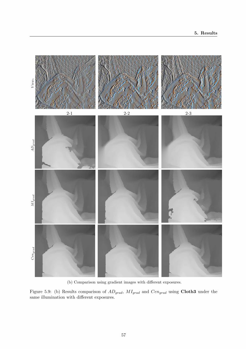
5. ResultsView
1
2-1 2-2 2-3
AD
grad
MI g
rad
Cen
grad
(b) Comparison using gradient images with different exposures.
Figure 5.9: (b) Results comparison of ADgrad, MIgrad and Cengrad using Cloth3 under thesame illumination with different exposures.
57

5. ResultsView
1
2-1 2-2 2-3
AD
int
MI i
nt
Cen
int
(a) Comparison using intensity images under different illuminations.
Figure 5.10: (a) Results comparison of ADint, MIint and Cenint using Cloth3 with the sameexposure under different illuminations. The notation l − r indicates different illumination com-binations, i.e., the left view captured under the l-th illumination is matched with the right viewcaptured under the r-th illumination. Thus, 2-2 means that the same illumination setting isused for both views in a stereo pair.
58

5. ResultsView
1
2-1 2-2 2-3
AD
grad
MI g
rad
Cen
grad
(b) Comparison using gradient images under different illuminations.
Figure 5.10: (b) Results comparison of ADgrad, MIgrad and Cengrad using Cloth3 with thesame exposure under different illuminations.
59

5. Results
5.2.3 Results on Airborne Image Sequence
One limitation of the Middlebury data sets is that all stereo pairs have relatively small baselines.In this subsection, using the airborne image sequence, we study the interdependency amongmatching performance and match costs by progressively changing stereo perspective. Ninecontinually recorded images build eight stereo pairs with an increasing baseline length from 35meters to 250 meters. The recorded urban region includes high buildings, wide and narrowstreets as well as large homogenous roof areas. Both bad-pixel and normalized median absolutedeviation (NMAD) are applied to describe the matching completeness and the deviation ofcorrect matching. We evaluate our results in three specific areas shown in Figure 5.11: the cityarea, the church roof area, and the building boundary area. The city area covers the wholeimage and allows a general evaluation. The roof area consists of a large and high church inorder to study the matching behavior in complicated situations like large homogenous surfacesand occlusions. The boundary area includes all building edges to analyze the discontinuitiesof a disparity map. The penalty factors P1 and P2 for each cost function are used based onparameter tuning of the Middlebury data and kept constant for all seven stereo pairs.
(a) (b) (c)
Figure 5.11: Evaluation masks on city and church area (a) and mask on boundary area (b). TheLiDAR ground truth is shown in (c).
Master 1 8
Figure 5.12: Cutdown in the church area. M denotes the master image, which is respectivelymatched with 1 and 8 that the stereo pair M-1 has the shortest baseline and M-8 has the longestbaseline.
To demonstrate the stereo perspective change during increasing the baseline length, a small
60

5. Results
cutout of the church area is shown in Figure 5.12. The master image is matched with thesequentially recorded images respectively. All images are captured by the nadir camera of the3K system. In total, eight stereo pairs covering the same area are evaluated.
Figure 5.13 illustrates the bad-pixel percentage and the NMAD of all individual cost functions(without merging) in the city area. The mis-match percentage (bad-pixel) decreases for allmatch costs from the first to the second stereo pair, because a too short baseline length causesa higher height error. After the second frame, the matching performance (NMAD) is slightlydecreased, but holds relatively steady for the next three stereo pairs. The reason for this isthat one the object similarities change during increasing the baseline length – the matchingperformance decreases, but statistically a matching result with relative large baseline length hasless ground deviations. From the fifth stereo pair (M-5), the bad-pixel percentage rises due tonotably changed observation views, particularly challenging for parametric costs like absolutedifference. Matching costs using gradient images show a higher sensitivity to baseline increasedue to uncertainties of edge locations. In general, census shows the highest robustness on theairborne images with increasing baseline length. Mutual information performs slightly betterthan census for stereo pairs with small baselines, but fails on data with large baselines, possiblydue to the Non-Lambertian reflectance.
As shown in Subsection 5.2.2.2, match costs based on gradient images are almost invariantto the radiometric changes. However, in contrast to the results on the Middlebury stereo sets,gradient based match show less stability when stereo pairs have a large baseline. In the remotesensing data, the facades of high buildings are observed differently in two views with largebaseline length, thus the gradients on objects boundaries are completely changed. Matchingusing gradient images is inferior to the intensity images. The similar behavior can not beobserved on stereo pairs with small baselines, like the Middlebury benchmark. Because gradientlocation shifts little, if the parallax changes only slightly.
Figure 5.13: Evaluation on the city area: indexes 1 to 8 denote the different matching pairswith increasing baseline. The Y-axis in the left diagram denotes of bad-pixel (height error morethan 5 meters). The Y-axis in the right diagram denotes the NMAD. Census shows the mostrobustness against the variation of parallax. Gradient based matching costs are more accuratethan their gray value variants, if the matching is successfully executed.
61

5. Results
Two stereo pairs (M − 2 and M − 8) are selected to observe the matching performancedifference during increasing baseline length. Census (Cenint), mutual information (MIint), andgradient based absolute difference (ADgrad) are compared in Figure 5.14 (We have not shownthe result of ADint, because this match cost is too sensitive to large stereo baseline.). Theresults using different cost functions on the stereo pair M − 2 with a small baseline length seemsimilarly, however, visible differences are measured on the results using the stereo pair M − 8with a large baseline length. While gradient based absolute difference fails completely on thestereo pair M − 8, census and mutual information perform well in different regions: censusgenerates more complete surfaces of homogenous regions; mutual information produces sharperedges on building boundaries. The robust performance of census in less texture areas is endowedfrom its window-based local support. But using neighbors for matching within a fixed windowsize causes blurring problem of census when apply it in discontinuity areas.
Cenint
M-2
MIint ADgrad
M-8
Figure 5.14: Results comparison between Cenint, MIint and ADgrad. The stereo pair, M-8, hasa larger baseline than M-2. Census shows the most robustness during increasing baseline length.In contrast, ADgrad performs well on M-2, but failed mostly on M-8. The edges generated byMIint are shaper then Cenint and ADgrad.
In the church area with less texture, cost functions using gradient images show more robust-ness and higher accuracy than using intensity images. This character is consistent with andmanifested on the Middlebury sets like Wood and Plastic. Absolute difference and mutualinformation are sensitive to radiometric changes and use only pixel-wise information for match-ing, hence, both of them fail mostly in the homogenous regions. Figure 5.13 shows the bad-pixelpercentage and the NMAD of different matching costs in the church area. In the homogenousregions of stereo pairs with large baselines, census using intensity images performs more robustthan gradient based absolute difference and mutual information. Note that, in Figure 5.13, thefailed matching with a large deviation is dealt as an outlier and is not counted in the evaluation,
62

5. Results
neither the bad-pixel percentage nor NMAD.Figure 5.16 illustrates the comparison using census, gradient based absolute difference and
mutual information on the church area. The Digital Elevation Models (DEMs) are generated bytheM−5 stereo pair. Compared with gradient based absolute difference and mutual information,census generates less noisy but loses the roof apex. On the building borders, census shows morecomplexness than the gradient based matching costs. To evaluate the matching performance,we apply the third mask on the boundary area.
Figure 5.15: Evaluation on the church area. Gradient based matching costs show the mostrobustness and the highest accuracy in this area, but the failed matching increases during in-creasing baseline length. AD and MI failed mostly in this area.
Cenint ADgrad MIgrad
Figure 5.16: Smoothness and completeness comparison on the church area. The left diagramshows the height values for Cenint, ADgrad and MIgrad along the profile indicated by the whiteline in the fist DEM. Compared with the gradient matching costs, Census generates less noisybut loses the roof apex.
Results on intensity images show mutual information produces sharper edges at discontinuityboundaries. In contrast, the size-fixed local support of census causes slightly blurred edges.Thus, the third mask is applied in order to detect matching performances of different on objectboundaries. Figure 5.17 presents the bad-pixel percentages of census, mutual information andtheir combination (MICint) respectively. Generally, mutual information performs better thancensus, but the errors of mutual information rise observably during increasing baseline length.
63

5. Results
MICint performs similar as MIint on data sets with short baselines and show also robustnesslike census when mutual information failed. The weight wMI of Mutual Information for thisevaluation is kept constant at 0.61 for all stereo pairs.
Figure 5.17: Evaluation on the boundary area. MI performs better than Census for the stereopairs with small baseline lengths. The lead of MI compared to Census disappeared by increasedbaseline length due to the higher robustness of Census. Failed matching of ADgrad and MIgradincreases observably, if the angle of view changes strongly, while Census and MI stay relativestable.
Since the different behaviors of mutual information and census depending on the baselines,we tuned the weight wMI from 0 to 1 with step 0.1 for each stereo pair during changing baselinelength, that the relationship between matching performance and cost functions depending onbaseline can be measured and manifested by the cost weight. Figure 5.18 demonstrates the erroranalysis of different weight parameters to combine mutual information and census (MICint). Theresult shows the larger the baseline of the stereo pair has, the smaller wMI performs better. Inother words, census performs better than mutual information on data with larger baseline. Theweight should be adapted to the observation constrains, like stereo baseline (adaptive MICint).The results of the statistical evaluation are shown in Table 5.5.
Figure 5.19 demonstrates the improvement through merging mutual information and census(MICint). In the boundary areas, MICint performs similarly as MIint generating sharp edgesand remains the completeness of census in the homogenous roof areas.
Finally, we illustrate results using mutual information, census and their combination witha fixed or adaptive weight parameter (fixed MICint and adaptive MICint) on the stereo pairswhen stereo baseline length increases as shown in Figure 5.21. Both mutual information andcensus perform well on stereo pairs with a small baseline length. However, Mutual informationfails gradually in the roof area during changing stereo perspective. In contrast, census can gen-erate less mis-matches then mutual information, even on stereo pairs with very large baselines.The merged matching cost, MICint with a fixed weight parameter, improves the matching per-formance, but still fails in the roof areas. Adaptive MICint, whose weight parameter is tunedaccording to the baseline length, shows the most robustness and the highest accuracy presented
1We use the weight parameter tuned by Middlebury data sets.
64

5. Results
in Table 5.5.
(a) (b)
Figure 5.18: MIC merged with fixed and adaptive weight. The left diagram illustrates thecomparison among MIC with fixed weight parameter wMI=0.6, MI and Cen. MIC performssimilar to MI on stereo pairs with small baselines, but keeps the robustness of Census for largerbaselines. The right diagram shows the weight tuning for wMI during increasing of baselinelength. The positions getting minimal error are projected at the Baseline-Weight surface andshow the weight trend.
M-1 M-2 M-3 M-4 M-5 M-6 M-7 M-8
w (35) (70) (105) (140) (175) (210) (245) (280)
0.0 23.8 20.7 19.8 18.7 18.7 18.5 18.7 18.80.1 23.9 20.5 20.0 18.4 18.7 18.4 18.7 18.70.2 23.6 19.7 19.4 18.4 18.5 18.2 18.9 18.70.3 23.4 20.3 19.5 18.1 18.4 18.2 18.7 18.50.4 22.6 19.5 19.5 17.9 18.2 18.5 18.7 18.70.5 22.4 20.1 18.4 17.9 18.1 18.2 18.6 18.60.6 21.7 19.7 18.4 17.8 18.0 18.0 18.7 18.80.7 22.2 19.7 18.1 17.9 18.3 18.2 18.5 18.90.8 21.6 19.9 18.8 18.1 18.2 18.5 19.1 19.20.9 22.5 18.9 18.2 18.2 18.8 18.8 19.2 19.51.0 21.9 19.2 18.6 18.6 19.3 19.4 20.0 20.5
Table 5.5: Evaluation of matching results in the boundary areas using MICint with differentwMI . Bad pixels are the percentage of mismatching compared with LiDAR points with an error> 5 meters. The red number in each column is the minimum error percentage and denotes thebest weight used.
65

5. Results
(a) (b) (c) (d)
Figure 5.19: Improvement by merging matching costs: MICint (d) generates sharper edges thanCenint alone (c) and constructs the high building completely which is lost using only MIint (b).One reference image is shown in (a).
5.2.4 Results on Satellite Data
A small cutout of the stereo data and the reconstruction results for an urban area (Terrassa inSpain, Barcelona) are shown in Fig. 5.20. The full data set covers mountainous, agricultural,forest, industrial and residential areas. The figure indicates that these images cannot be matchedsuccessfully using Mutual Information, while Census and the MICint perform reasonably wellon this challenging data set. The large black background in the Mutual Information imagewas incorrectly filled using this data. Table 5.6 shows the results of evaluating the city areashown in Fig. 5.20 and two other test areas (hilly forest and industrial area) against the LiDARreference data. It is clearly visible that MICint performs slightly better than Census and thatMutual Information does produce the largest errors. Experiments with various values for P1, P2
and WP2 indicated that performance depends mainly on the cost function and not on the exactparametrization of the stereo algorithm.
Cost P1 P2 WP2 wMI NMAD Bad pixels
MICint 700 1400 200 0.3 0.72 15.8 %Cenint 600 1300 200 - 0.74 16.8 %MIint 700 1400 200 - 1.10 25.8 %
Table 5.6: Evaluation of Matching results in three test areas using ground truth LiDAR Data.NMAD is the normalized median deviation and Bad pixels is the percentage of pixels with anabsolute height error > 2 m.
66

5. Results
Figure 5.20: Small cutout of the Worldview-1 Stereo pair. First column: stereo pair and LiDARreference data. Second column: Results after stereo matching with different cost functions,orthographic reprojection and discontinuity preserving interpolation.
67

5. Results
Figure 5.21: Disparity maps for stereo pairs with increasing baseline. The images 1 to 8 arematched with the center image C respectively b. The results for MI, Census, MIC and adaptiveweighted MIC are shown in columns 2-5. The black areas indicate failures of the left-right check.
bNote that the shown reference images are not rectified.
68

5. Results
5.2.5 Discussion
In this section we investigate the interdependencies among matching performance, match costfunctions, and observation constraints using both the standard benchmark and remote sensingdata sets. We summarize our study under four criteria as follows:
• Insensitivity to radiometric changes: Although absolute difference and Mutual Infor-mation perform well on Middlebury data under good radiometric conditions and remotesensing data with small baseline lengths, they fail mostly on Middlebury data with ra-diometric changes and remote sensing data with long baseline due to non-Lambertianreflectance. In contrast, census shows the highest robustness on both close-range datawith radiometric changes and almost all used remote sensing data. Cost functions appliedto gradient images are generally insensitive to radiometric changes and perform well onMiddlebury data and remote sensing data with short baseline length.
• Robustness during increasing baseline length and stereo angles: Except non-Lambertian reflectance, one most challenge for stereo pairs with long baseline and largestereo angle is notable object shape change between left and right view, an extreme exampleis the facade area of a high building. This challenge causes location shift of gradients thatmatching costs using gradient images mostly fail. Mutual information applied to intensityimages performs better as absolute difference on airborne stereo pairs with long baselines,but fails completely on the satellite data with very large stereo angles. Census achievesthe highest robustness both on airborne and satellite images.
• Completeness in homogenous areas: Our evaluation shows that the matching perfor-mance of cost functions depends not only on the observation conditions, but also on theimaged areas. Regions with less texture impede matching by high ambiguities. Pixel-wisecosts applied on gradient images show more completeness than the directly using intensityimages, probably due to non-labertian reflectance. The bit-wise recording of census detectsthe relative relationship between the local ambiance and restricts outliers in small valuethat Census outperforms Absolute Difference and Mutual Information in these areas.
• Blurring in discontinuity regions: Cost functions applied to gradient images generaterugged edges due to location shifts of gradients in two stereo-views. In addition, thewindow-based local support of census causes blurring in discontinuity regions both onMiddlebury data and airborne images. However, pixel-wise costs using intensity imagesshow more accuracy in the object boundaries and sharper edges are reconstructed.
• Contribution of merging matching costs: The influence of data on matching performanceshows, there is no almighty matching cost for all data in all regions. Merging differentcosts profits their individual advantages to improve the matching performance. In ourevaluation, the cost combination using mutual information and census performs similarlyas absolute difference and mutual information in large discontinuity area and as robust ascensus both in homogenous area and on data with large stereo angles.
69

5. Results
5.3 Evaluation of the Confidence-based Surface Prior
In this section we evaluate the confidence-based surface prior and compare it with existingsegment-based methods. Both the Middlebury benchmark and the 3K+ airborne stereo pairsare used. In our evaluation, the advantages of adding the confidence-based surface prior intoa global framework are highlighted: We analyze the discontinuities along object boundariesto demonstrate sharper edges through the surface prior; Texture-rich stereo pairs are selectedto show the decreasing sensitivity of our prior to a given segmentation; The profile througha building roof shows the improved matching completeness using the surface prior on largehomogenous regions.
5.3.1 Results on Middlebury Benchmark
Table 5.7 demonstrates the quantitative improvement when applying our surface prior on theMiddlebury online benchmark. Compared with our SGM implementation, improvement is ob-tained under all criteria for all four datasets. Figure 5.22 demonstrates the result comparisonbetween SGM and our iSGM3 on Teddy and Cones from the Middlebury online benchmark.The dilation of the chimney and Teddy bear are reduced in (c) in contrast to (b). The meshbackground is better defined and edges are sharper in (c). Our results perform similar as thework using soft surface prior [Woodford et al., 2009] except the result of Venus, because oursegmentation is not tuned for the online benchmark. It seems, color segmentation works well onthese four data sets, thus the methods using segmentation-based hard constraint perform verywell [Sun et al., 2005; Wang and Zheng, 2008]. However, as shown in Figure 4.1, methods usinghard plane constraint are extremely sensitive to the given segmentation. Oft over-segmentationis required. In texture-rich regions, artifacts from segmentation can appear.
Algorithm Tsukuba Venus Teddy Conesnocc all disc nocc all disc nocc all disc nocc all disc
iSGM3 2.40 3.16 10.1 1.47 2.49 14.2 10.2 16.3 21.4 4.2 11.4 12.7
SGM 2.73 3.60 11.4 2.0 3.32 15.9 12.1 18.0 23.2 5.41 13.5 13.8
2OP+occ 2.91 3.56 7.33 0.24 0.49 2.76 10.9 15.4 20.6 5.42 10.8 12.5
SymBP 0.97 1.75 5.09 0.16 0.33 2.19 6.47 10.7 17.0 4.79 10.7 10.9
DoubleBP 0.88 1.29 4.76 0.13 0.45 1.87 3.53 8.3 9.63 2.9 8.78 7.79
Table 5.7: Evaluation of bad-pixel percentage on Middlebury online benchmark with ErrorThreshold > 1. Our SGM results differ from Hirschmuller [2008] due to different match costfunction and post processing for filling occlusion holes used in our implementation. The iSGM3performs similar as 2OP+occ [Woodford et al., 2009] except the result of Venus, probably dueto the color segmentation used. Methods using hard segment-based constraint like SymBP [Sunet al., 2005] and DoubleBP [Wang and Zheng, 2008] show the best performance on these data.
Furthermore, figure 5.23 demonstrates improved accuracy when utilizing our surface prioron more images from the Middlebury datasets other than the online benchmark. The proposedconfidence-based surface prior converts the hard segment-based constraint from the plane-fitdisparity map into a soft prior that is not as reliant on the plane-fit disparity. Sharp edges andsloped surfaces can be generated naturally via a global energy minimization without the hardconstraint imposed by plane-fit disparity. For instance, the open book in Baby2 is texture-lessand has a smoothly bowed surfaces in the disparity space. The result without our prior contains
70

5. Results
(a) Reference images (b) SGM (c) iSGM3
Figure 5.22: Comparison on Middlebury online benchmark. We compare the disparity results,after left-right consistency checking, with and without the proposed soft prior. Top: Thedilation of the chimney and Teddy bear are reduced in (c) in contrast to (b). Bottom: Themesh background is better defined and edges are sharper in (c).
large miss-matched areas due to texture homogeneity. In contrast, the hard segmentation-basedconstraint enforces a single slanted plane for the book, which is not in consistent with theground truth. In contrast, our surface prior allows the faithful reconstruction of the bookssurface. As edges of objects boundaries and slanted planes in the disparity maps of Reindeerand Lampshade1 benefit from the hard plane constraints, Cloth3 with rich textures andsmoothly varying depth is cut apart by the segments artifacts. The hard constraint enforceseach segment as a disparity plane instead of a segmentation-independent smooth surface. Ourconfidence-based prior improves shape edges and slanted surfaces, but still remains good resultsfrom initial matching.
Algorithm Baby2 Reindeer Lampshade1 Cloth3nocc all disc nocc all disc nocc all disc nocc all disc
iSGM3 10.4 12.3 14.1 14.0 17.6 22.5 13.6 14.5 18.8 3.6 4.2 5.5
SGM 17.3 19.3 21.6 19.3 25.3 31.2 16.3 18.1 21.2 3.6 4.2 5.5
Plane-fit 15.9 17.5 24.3 12.2 18.8 21.8 13.2 14.4 18.4 17.5 18.7 29.7
Table 5.8: Evaluation on the Middlebury data sets with bad-pixel error threshold > 1. Theresults are shown in Figure 5.23.
Our confidence-based surface prior differs from existing surface constraints in that it variesthe per-pixel strength of the constraint to be proportional to the confidence in our given dis-parity estimation. In contrast to many methods using soft surface priors [Bleyer et al., 2010;Woodford et al., 2009], the proposed confidence measure for our surface prior is calculated from
71

5. Results
(a) Reference im-ages.
(b) Results with-out our soft surfaceprior.
(c) Plane-fit dis-parity from (b).
(d) Results withour soft surfaceprior.
(e) Ground truth.
Figure 5.23: Comparison on Middlebury 2005 and 2006 data sets. Top (Baby2): Discretedisparity levels in the low-texture curved book surface in (c) is partially smoothed out in (d).The baby doll is also better reconstructed in (d). Top-mid (Reindeer): The blue foregroundrope is reconstructed better in (d) than in (b) or (c), and the brown head/mask has betterdefined edges in (d) than in (b). Bottom-mid (Lampshade1): Both the thin stick and largesurfaces are better reconstructed in (d). Bottom (Cloth3): Our surface prior performs robuston texture-rich data. (b) and (d) are almost identical, as segmentation artifacts are observed in(c).
an energy minimization without reference to planar surfaces or regions. Thus it is independentof the plane fitting process. Using this confidence, the Gaussian interpretation of the plane-fitresult in energy space makes our surface prior more robust to segmentation errors. To demon-strate the effectiveness of our confidence measure we compare disparity maps produced by ourproposed confidence-based Gaussian surface prior and the soft surface prior defined using dis-parity distance between δp and dp in Figure 5.24. Absent scaling by our confidence measure,the soft surface prior causes the reconstruction of the bowling ball to be relatively planar invertical stripes. The round shape of the bowling ball is correctly reconstructed when using theconfidence-based surface prior.
In contrast to real-world data, color segmentation works well on the Middlebury data sets.This is the main reason, why many segment-based methods reach high ranks of the online bench-mark. However, effects like object shadowing, which often appear in real-world applications, arenot included. Such failed color segments can lead to critical results. For instance, a building
72

5. Results
(a) (b) (c)
(d) (e) (f)
Figure 5.24: Comparison of simple disparity distance prior and the confidence-based prior onBowling2: (a) Reference image. (b) Ground truth. (c) Result without soft prior: matchingon the boundary areas of objects failed a bit. But the shape of the ball is well reproduced. (d)Plane-fit disparity from (c): The ball is reconstructed as a set of vertical stripes, and the pin hasbecome poorly defined. (e) Result using soft prior without confidence: Edges are well defined,but some vertical striping of the bowling ball remains. (f) Result using our surface prior: Therounded shape of the ball is better reconstructed than in (e) and the edges are shaper than in(c).
facade is assigned in the same segment with its shadow on street, hard plane constraint enforcesa slanted plane connecting the roof and the street, instead a perpendicular wall. In the nextsubsection, we show more contrast between our approach and segment-based method .
73

5. Results
5.3.2 Results on Airborne Stereo Pairs
Non-lambertian reflectance and scene complexity all combine to make dense stereo matching onreal-word data challenging in contrast to the Middlebury benchmark. The airborne 3K+ datainclude large homogenous roofs, high buildings, small streets, regions under shadows as wellas moving pedestrians and vehicles. The lighting environment of typical airborne imagery isdynamic – the sun can be hidden by clouds of short duration. In this subsection we demonstrateresults of our algorithm on airborne stereo pairs in an urban area. Obvious improvements inaccuracy are obtained by our proposed algorithm: sharp building edges, complete roof regions,and less noise on the streets. Building boundaries benefit most from our method. They areimportant features, but cover only a small percentage of the whole image. Thus, we havemanually generated building-edge segments to evaluate the disparity changes within a smalllocation. This evaluation highlights the robustness of our surface prior when applied for a real-world scene. In addition, we use also stereo pairs with large baselines. For a fair comparison,we use the truncated absolute difference, both for both SGM and iSGM3.
We focus now on the stereo pairs with short baseline. The bad-pixel percentages of SGM andiSGM3 are very similar, 18.76% for SGM and 18.74% for iSGM3. In contrast to the comparisonusing the Middlebury data, the difference between both methods is not clear. There are severalreasons for this: (1) The resolution of our groundtruth is much lower than the 3K+ images; (2)The 3K+ images were captured seven years after the groundtruth laser scanning. During theseyears, many buildings are were torn down and rebuild; (3) We observe that object boundariesbenefit mostly from iSGM3 on this data set, but these cover only a small percentage of the image.However, Figure 5.25 shows two cutouts to compare results with or without the surface prior.Many mis-matches are observed on roofs, facades and streets where pedestrians are moving.Plane-fit method revamps hardly the building boundaries at cost of segment artifacts (shown asregions of black holes). In contrast, results using iSGM3 contain less mis-matches and no fittingartifacts.
Figure 5.26 shows the superior performance of our method on large homogenous regions.Along the indicated white arrow through the large homogeneous church roof area, we demon-strate the improvement obtained by our confidence-based surface prior in (c). In contrast to alot of unreliable disparities after consistency checking on the disparity map without applying oursoft surface prior 6, a smooth and gradual changing roof is reconstructed when incorporating ourconfidence-based surface prior. Additionally, the church edges are perfectly generated withoutany dilation into the shadowed streets below.
In order to evaluate the disparity changes on object boundaries, we manually generatededge segments shown as green masks in Figure 5.27 (b). Edges are selected, if the heightdifference beside them are very high. Figure 5.27 (a) explains the evaluation procedure usingthese edge masks. Given a small location threshold, disparities of pixels along the normals of themasks are compared. Only if the disparity change are higher than another disparity threshold,we count this location as a disparity discontinuity. The amount of discontinuities is dividedby the pixel number of edges. A high percentage indicates that the disparity map has sharpedges. Five location thresholds from 1 pixel to 5 pixels are used. The disparity threshold isselected as 15 pixels difference at least. Table 5.9 demonstrates the comparison between SGM,iSGM3 and plane-fit generated disparity maps. Our surface prior perform superiorly in thelarge discontinuity regions. The hard constraint of plane-fit generates many artifacts, becausesegments near building boundaries often include some shadow regions on streets. In contrastto the bad-pixel evaluation of the whole image, the performance difference between results withand without our surface prior is very clear.
74

5. Results
(a) (b) (c) (d)
Figure 5.25: Results on airborne images: (a) Reference images. (b) Results without surface-prior (SGM). (c) Plane-fit disparity maps from (b). (d) Our results (iSGM3)
Method Threshold = 1 2 3 4 5
SGM 24.03% 36.89% 48.94% 61.63% 74.75%Plane− fit 10.34% 12.50 % 13.39% 17.97% 20.44%iSGM3 36.76% 48.03% 59.16% 70.20% 83.25%
Table 5.9: Evaluation using edge masks. The location thresholds are selected from 1 pixelto 5 pixels along the normals of edges. iSGM3 performs better than SGM in all thresholds.Especially, the difference of the small thresholds is clear that results using the surface priorcontain shaper edges. The plane fit results suffer from bad segmentation at object boundarieswith shadows.
We evaluate the surface prior also on airborne images with large baselines. In Figure 5.28, themaster image (M) is matched with the reference images 1 (short baseline) and 2 (long baseline).The rows, (a), (b), and (c) present the results without our soft region prior, of the plane-fitting of(a), and with our confidence-based soft surface prior, respectively. Matching on the M-2 stereopair is much more difficult than the M-1 stereo pair due to the increased baseline separation.Even on the stereo pair with a large baseline, the contribution of our confidence-based softsurface prior is clear: more complete roofs, clear boundaries, and fewer outliers.
5.3.3 Discussion
In this section we compare the results with and without the confidence-based surface prior usingboth the Middlebury benchmark and the airborne stereo pairs. The iSGM3 uses a very similarenergy minimization framework like SGM, the only difference between them is that we fuse costsfrom a plane-fit result into the aggregated match cost. However, results using the additional prior
75

5. Results
(a) Reference image. (b) Result without our surface prior (SGM).
(c) Profile of disparity change. (d) Result with our surface prior (iSGM3).
Figure 5.26: Comparison of results on the airborne images. (b) Without our surfaceprior there is a lot of false matching on the street level and homogeneous roof regions. Thereconstructed building edges are dilated into the shadow areas. (c) With our surface prior,accuracy is improved in all surface areas, building edges, and roof areas when compared with(b). (d) Profile on the homogeneous church roof area. The profile shows the disparity changealong the indicated white arrow both with (blue line) and without (green line) our surface prior.The use of our surface prior reconstructs a closer approximation to the roof surface, without theextreme outliers observed in (b). Additionally, the building edges are sharper when our surfaceprior is utilized.
contain shaper edges and more complete surfaces than results using energy minimization onlyincluding data and smoothness terms. This fact – improvement by adding high-level priors likesurface prior even using the same optimization framework – inspires us to make joint inferencesbetween stereopsis and object recognition (see Future Work).
76

5. Results
DisparityDisparity
Disparity changewithin the threshold
LocationThreshold
(a) (b)
Figure 5.27: Evaluation using edge masks (a) Evaluation procedure: The blue shapes denotethe reconstructed building facades. Disparity changes are calculated within a small locationthreshold (shown as red lines). (b) Edges masks of a rectified airborne image: The edgessegments shown as green lines are selected on the building sides in order to check the largediscontinuities besides the lines in a disparity map.
In addition, this evaluation indicates that region-based methods are preferable around objectboundaries and in large homogeneous areas; the use of object regions can propagate strongmatches into sub-regions where poor matches appear. However, defining an energy minimizationover regions, rather than pixels, imposes a hard constraint that forces depths to lie on the smoothsurface associated with a region; removing fine-level details from the depth map in the process.The results are very sensitive to the given segmentations. In contrast, our prior learns thestrength of a pixel lying on a surface from the previous result and fuses this cost with matchcost and smoothness penalties together. The semi-global framework aggregates the fused costspath-wise. Thus, the artifacts of a plane-fit disparity map are avoided.
5.4 Summary
In this chapter the interdependencies among matching performance, cost functions, and ob-servation conditions are investigated using both close-range and remote sensing data: MutualInformation performs well on stereo pairs with global radiometric changes. Non-parametricmatch costs like Census works robust in texture-less regions and on stereo pairs with largebaseline. Based on this study, the cost-merging strategy is developed in order to combine theadvantages of different match cost functions and gives consideration to imagery configurations.
In the second part of this chapter, a confidence-based surface prior is introduced for globalenergy minimization. This surface prior varies in the existing hard segment-based priors, whichforce each pixel belonging to a spatial surface. In this work the hard plane-fitting result ismodeled as a distribution using the previous (aggregated) match costs. Thus, segmentationartifacts can be effectively avoided. Moreover, the addition of this prior has shown more benefits:sharp object-boundary edges in areas of depth discontinuity; and accurate disparity in surfaceregions.
77

5. Results
M 1 2
M-1(a) M-1(b) M-1(c)
M-2(a) M-2(b) M-2(c)
Figure 5.28: Comparison on stereo pairs with increasing baselines. M denotes the master image,which is rectified and matched with a short baseline (1) and long baseline (2) image. M-x(a)presents the results without our soft surface prior. M-x(b) are the plane-fit disparity maps toM-x(a). M-x(c) are the results with our soft surface prior.
78

Chapter 6
Conclusion and Outlook
The goal of this dissertation is to develop robust stereo matching method for challenging real-world data. To this end, we conduct two components of the global stereopsis frameworks: therobust match cost functions and the addition of the confidence-based surface prior in globalenergy formulations.
Match cost is the most fundamental component for correspondence computations. All stereomethods use a cost function to compute the similarity of possible correspondences. To developreliable match costs, we investigate into the interdependencies among matching performance,cost functions, and observation conditions. Parametric, non-parametric match costs, and thematch cost based on mutual information are evaluated and compared in context of data (radio-metric changes, object features) and observation conditions (stereo baselines). Both close-rangeand remote-sensing data are used. The analysis in this dissertation indicates that there is nosingle cost function that performs best for all circumstances. Instead, the match cost functionhas to be chosen based on the properties of imagery conditions and data applied. We introducesome general guidelines for choosing suitable match cost functions:
• Parametric match costs and mutual information allow accurate reconstruction of fine de-tails, such as building edges, but lead to increased sensitivity to radiometric changes.
• Non-parametric match costs encode image local structures, which improves robustness,but leads to reduced accuracy on fine details and edges.
• The matching performance of a cost function depends on observation constraints such asbaseline length. For stereo pairs with large baselines, non-parametric costs perform morerobust than parametric match costs and mutual information.
• Features (homogeneity, discontinuity, visibility, etc.) of imagery objects confront matchcosts with a variety of challenges. For example, in texture-less regions, non-parametricand window-based cost functions are suggested.
For these studies, we apply both standard benchmarks and challenging remote sensing datasets. We demonstrate the challenges such as non-Lambertian reflectance, complex scene, andradiometric changes in real-world applications. Our investigation on match costs indicates thatdifferent match cost functions are complementary in different situations. Thus, we contribute acost-merging strategy with respect to the stereo baseline length, in order to combine advantagesof different cost functions and improve matching performance in robustness and accuracy.
Currently almost all of the best stereo-matching algorithms are framed as global energyminimizations, which aim to solve the stereopsis using some regularizer – typically the smooth-ness of resulting disparity maps. However, such energy optimization is computed pixel-wisely
79

6. Conclusion and Future Work
– both the cost calculation and the energy propagation. High-level priors are oft completelymissing. The experience of a lot of researchers indicate that segment-based methods are prefer-able around object boundaries and in large homogeneous areas; the use of color segments helpspropagate strong matches into sub-regions with poor matches. However, defining an energyminimization over segments, rather than pixels, imposes a hard constraint that forces depths tolie on the smooth surface associated with a region; removing fine-level details from the depthmap in the process. The results are very sensitive to the given segmentations. Thus, in thisdissertation we introduce a novel confidence-based surface prior for energy minimization formu-lations of dense stereo matching. Given a dense disparity estimation we fit planes, in disparityspace, to regions of the image. For each pixel, the probability of its depth lying on an objectplane is modeled as a Gaussian distribution, whose variance is determined using the confidencefrom a previous matching. We then recalculate a new disparity estimation with the additionof our novel confidence-based surface prior. The process is then repeated. Unlike many region-based methods, our method defines an energy formulation over pixels, instead of regions in asegmentation; this results in a decreased sensitivity to the quality of the initial segmentation.The introduced confidence-based surface prior differs from existing surface constraints in thatit varies the per-pixel strength of the constraint to be proportional to the confidence in thegiven disparity estimation. Based on the experiment of this dissertation, useful and generalconceptions for global stereopsis methods are summarized:
• Energy function formulation with additional object-level prior. Standard energy formula-tions using data and smoothness terms have reached their limitation of matching perfor-mance. High-level priors can inject semantical knowledge of the physical world into thegoal function. However, addition of high-level priors leads oft to a hard constraints andgenerates artifacts.
• Pixel-wise energy optimization. To solve the global energy function, optimization shouldbe operated over pixels. Optimization methods, which are not defined in pixel space,often impose hard constraints. Once a mis-match (in fact, a large region of mis-matches)appears, it is very difficult to eliminate it.
• Probabilistic costs fusion. An efficient way to combine additional costs into aggregatedmatch costs is to build a probabilistic framework such that the hard constraint can berelaxed in the energy optimization.
• Iterative processing. The knowledge about the unknown result can only be groped in agradual manner. Iterative methods allow an update or/and addition of high-level priorsinto the processing step-by-step.
As a concrete realization iSGM3 is introduced in this work. This iterative pixel-wise energyminimization method solves energy function defined with data, smoothness and surface priors.The cost aggregation of iSGM3 is similar to SGM and the penalty for surface constraint isfused with the path-wise aggregated costs. The addition of the confidence-based surface priorhas three main benefits: sharp object-boundary edges in areas of depth discontinuity; accuratedisparity in surface regions; and low sensitivity to segmentation.
Thus, our goal – developing stereo methods for challenging data – is achieved by the costmerging strategy depending on the baseline length and the confidence-based surface prior in-corporating a novel energy optimization method. Both novelties are generally applicable foralmost all extended stereo methods. The ideas behind our contributions may guide researchersto develop their own algorithms.
80

6. Conclusion and Future Work
6.1 Outlook
Dense stereopsis formulated as a global energy minimization problem has been intensely investi-gated since last decade. Regarding to different components in global frameworks, there are stillmatch costs functions remain to be investigated. There are also many optimization algorithmsthat might be considered by designing stereopsis method. This dissertation aims at developingnew stereo methods that solve two problems: less robustness of match costs and absence ofsemantic information about the scene to be reconstructed. However, three main perspectivesare of special interest for future research:
• Stereo matching based on superpixels. Over-segmentation is required for manyexisting segment-based stereo matching methods. Although the proposed iSGM3 using aconfidence-based surface prior is less sensitive to a given color segmentation, artifacts doappear in segments of large areas. Superpixels can be used to replace the rigid structureof the pixel grid [Radhakrishna Achanta and Suesstrunk, 2012]. The sizes of superpixelsshould be smaller as color segments and more similar with each other. Moreover superpixelsshould adhere well to image boundaries and reduce computational complexity.
• Jointly solves for depth and image segments. In this dissertation color segmentationis once generated and used for the iterative processing. In fact a depth map can also beused in order to improve a segmentation in image space. Grouping or splitting segmentswith respect to the spatial depth-boundaries may modify incorrect segments, especially intexture-rich regions. The segmentation and depth estimation might be formulated as ajoint energy minimization problem that energy of each pixel is the sum of energies encodingshape appearance and depth, taking special care into modeling occlusions [Yamaguchiet al., 2013].
• Object detection and tracking using disparity maps. Depth maps generate a newview of the scene. In contrast to object tracking in image space which requires detectingfeatures and determining their correspondences, object boundaries can be better detectedand tracked using disparity. Moreover, extracted disparity forms can be used to matchgeometric model of objects to identify interesting regions before tracking.
What makes the stereopsis interesting are its applications. For instance, stereo camerasystems are used for recognizing road surface undulations in advance that the suspension of ego-vehicle can be adjusted to suit the situation [Kruse, 2014]. However, very challenging real-worlddata as shown in the work of Meister et al. [2012] are only restricted solvable due to the physicallimitations of optical systems. In the future, to develop highly robust and accurate perceptionsystems for understanding dynamical environments,´we will be applying additional sensors likeradar/laser-scanner and fusing their data with stereo systems.
81

Appendix A: Data Set
Aloe Art Baby1 Baby2 Baby3
Books Bowling1 Bowling2 Cloth1 Cloth2
Cloth3 Cloth4 Dolls Flowerpots Lampshade1
Lampshade2 Laundry Midd1 Midd2 Moebius
Monopoly Plastic Reindeer Rocks1 Rocks2
Wood1 Wood2
Figure 6.1: Left reference images of the used Middlebury data.
82
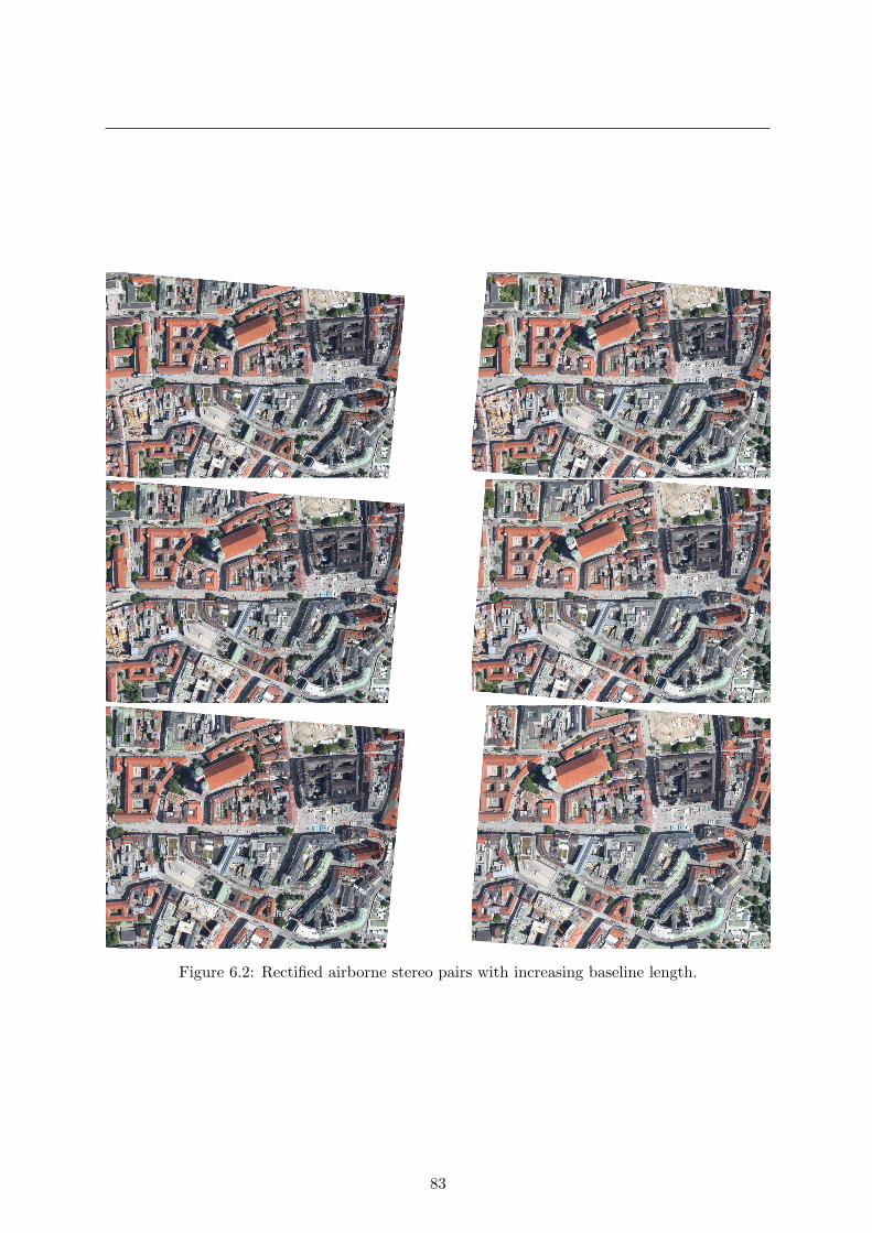
Figure 6.2: Rectified airborne stereo pairs with increasing baseline length.
83

References
Tarkan Aydin and Yusuf Sinan Akgul. Stereo depth estimation using synchronous optimizationwith segment based regularization. Pattern Recognition Letters, 31(15):2389–2396, November2010. 35
H. H. Baker and T. O. Binford. Depth from edge and intensity based stereo. In InternationalJoint Conference on Artificial Intelligence, pages 631–636, 1981. 19
Christian Banz, Sebastian Hesselbarth, Holger Flatt, Holger Blume, and P. Pirsch. Real-time stereo vision system using semi-global matching disparity estimation: Architecture andfpga-implementation. In 2010 International Conference on Embedded Computer Systems(SAMOS), pages 93–101, 2010. 19
Christian Banz, Peter Pirsch, and Holger Blume. Evaluation of penalty functions for semi-globalmatching cost aggregation. In XXII ISPRS Congress, 2012. 18, 36
Adrian Barbu and Song-Chun Zhu. Generalizing swendsen-wang to sampling arbitrary posteriorprobabilities. IEEE Transactions on Pattern Analysis and Machine Intelligence, 27(8):1239–1253, 2005. 16
Stephan Barnard. Stochastic stereo matching over scale. International Journal of ComputerVision, 3(1):17–32, 1989. 16
Benedichte Bascle and Rachid Deriche. Stereo matching, reconstruction and refinement of 3dcurves using deformable contours. In International Conference on Computer Vision, pages421–430, 1993. 19
A. Bensrhair, P. Miche, and R. Debrie. Fast and automatic stereo vision matching algorithmbased on dynamic programming method. Pattern Recognition Letters, 17:457–466, 1996. 17
Julian Besag. Spatial interaction and the statistical analysis of lattice systems. Journal of theRoyal Statistical Society, 36(2):192–236, 1974. 14
S. Birchfield and C. Tomasi. A pixel dissimilarity measure that is insensitive to image sampling.PAMI, 20(4):401 – 406, 1998. 22
S. Birchfield and C. Tomasi. Depth discontinuities by pixel-to-pixel stereo. International Journalof Computer Vision, pages 269–293, 1999. 17
M. Bleyer and M. Gelautz. Graph-based surface reconstruction from stereo pairs using imagesegmentation. In SPIE, volume 5665, pages 288–299, 2005. 1, 15
84

REFERENCES
Michael Bleyer, Carsten Rother, and Pushmeet Kohli. Surface stereo with soft segmentation.In CVPR, pages 1570 – 1577, 2010. 33, 34, 35, 71
Michael Bleyer, Carsten Rother, Pushmeet Kohli, Daniel Scharstein, and Sudipta Sinha. Objectstereo — joint stereo matching and object segmentation. In CVPR, pages 3081 – 3088, 2011.33, 35
A. F. Bobick and S. S. Intille. Large occlusion stereo. International Journal of Computer Vision,33(3):181–200, 1999. 11
Y. Boykov, O. Veksler, and R. Zabih. A variable window approach to early vision. IEEETransactions on Pattern Analysis and Machine Intelligence, 20(12):1283–1294, 1998. 26
Y. Boykov, O. Veksler, and R. Zabih. Fast approximate energy minimization via graph cuts.IEEE Transactions on Pattern Analysis and Machine Intelligence, 23(11):1222–1239, 2001. 1
Yuri Boykov and Vladimir Kolmogorov. An experimental comparison of min-cut/max-flowalgorithms for energy minimization in vision. PAMI, 26(9):1124–1137, 2004. doi: 10.1109/TPAMI.2004.60. 16, 36
A.T. Brint and M. Brady. Stereo matching of curves. Image and Vision Computing, 8(1):50–56,1990. 19
Alan Brunton, Chang Shu, and Gerhard Roth. Belief propagation on the gpu for stereo vision.In Canadian Conference on Computer and Robot Vision, pages 26–26, 2006. 16
Xuanping Cai, Dongxiang Zhou, Ganhua Li, and Zhaowen Zhuang. A stereo matching algorithmbased on color segments. In International Conference on Intelligent Robots and Systems,volume 3372 -3377, 2005. 35
D. Chandler and J. K. Percus. Introduction to modern statistical mechanics. Physics Today,41, 1988. 16
Huahua Chen. Stereo matching using dynamic programming based on occlusion detection. InInternational Conference on Mechatronics and Automation, 2007. 17
R. Chrastek and J. Jan. Mutual information as a matching criterion for stereo pairs of images.Analysis of Biomedical Signals and Images, 14:101–103, 1998. 22
Dorin Comaniciu and Peter Meer. Mean shift: A robust approach toward feature space analysis.PAMI, 24(5):603 – 619, 2002. doi: 10.1109/34.1000236. 36
Juan Jose de Dios and Narciso Garcia. Face detection based on a new color space ycgcr. InInternational Conference on Image Processing, volume 3, pages 909–12, 2003. 24
R. Deriche and O. Faugeras. Tracking line segments. In European Conference on ComputerVision, 1990. 19
Geoffrey Egnal. Mutual information as a stereo corresponce measure. In Computer and Informa-tion Science, number Technical Report MS-CIS-00-20. University of Pennsylvania, Philadel-phia, USA, 2000. 27
F. Forbes and G. Fort. Combining monte carlo and mean-field-like methods for inference inhidden markov random fields. IEEE Transactions on Image Processing, 16:824–837, 2007. 16
85

REFERENCES
Sven Forstmann, Yutaka Kanou, Jun Ohya, Sven Thuering, and Alfred Schmitt. Realtimestereo by using dynamic programming. In IEEE Conference on Computer Vision and PatternRecognition Workshop, pages 29–29, 2004. 16, 17
Andrea Fusiello, Emanuele Trucco, and Alessandro Verri. A compact algorithm for rectificationof stereo pairs. Machine Vision and Applications, 12:16–22, 2000. 8, 9
Stefan Gehrig and Clemens Rabe. Real-time semi-global matching on the cpu. In IEEE Com-puter Society Conference on Computer Vision and Pattern Recognition Workshops, pages85–92, 2010. 19
Stefan Gehrig, Felix Eberli, and Thomas Meyer. A real-time low-power stereo vision engine usingsemi-global matching. In Computer Vision Systems, volume 5815, pages 134–143. LectureNotes in Computer Science, 2009. 19
Stefan K. Gehrig and Uwe Franke. Improving stereo sub-pixel accuracy for long range stereo.In International Conference on Computer Vision, 2007. 17
A. Geiger, M. Roser, and R. Urtasun. Efficient large-scale stereo matching. In Computer Vision- ACCV2010, volume 6492 of Lecture Notes in Computer Science, pages 25–38, 2010. 19, 20
S. German and D. German. Stochastic relaxation, gibbs distributions, and the bayesian restora-tion of images. IEEE Transactions of Pattern Analysis and Machine Intelligence, 6:721–741,1984. 13, 16
Minglun Gong and Ruigang Yang. Image-gradient-guided real-time stereo on graphics hardware.pages 548–555, 2005a. doi: 10.1109/3DIM.2005.55. 36
Minglun Gong and Yee-Hong Yang. Fast stereo matching using reliability-based dynamic pro-gramming and consistency constraints. In ICCV, volume 1, pages 610 – 617, 2003. doi:10.1109/ICCV.2003.1238404. 36, 38
Minglun Gong and Yee-Hong Yang. Near real-time reliable stereo matching using programmablegraphics hardware. In CVPR, volume 1, pages 924–931, 2005b. doi: 10.1109/CVPR.2005.246.11, 17, 26
Minglun Gong, Ruigang Yang, Liang Wang, and Mingwei Gong. A performance study ondifferent cost aggregation approaches used in real-time stereo matching. IJCV, 75(2):283–296, 2007. 11, 23
J.Y. Goulermas and P. Liatsis. A new parallel feature-based stereo-matching algorithm withfigural continuity preservation, based on hybrid symbiotic generic algorithms. Pattern Recog-nition, 33:529–531, 2000. 19
W. E. L. Grimson. Computational experiments with a feature based stereo algorithm. IEEETrans. On Pattern Analysis Machine Intelligenz, 7(1):17–34, 1985. 19
I. Haller, C. Pantilie, F. Oniga, and S. Nedevschi. Real-time semi-global dense stereo solutionwith improved sub-pixel accuracy. In IEEE Intelligent Vehicles Symposium, pages 369–376,2010. 18
R. M. Haralick and L. G. Shapiro. Computer and robot vision. Addison-Wesley LongmanPublishing Co., Inc., Boston, 1992. 8
86

REFERENCES
Yong Seok Heo, Kyoung Mu Lee, and Sang Uk Lee. Illumination and camera invariant stereomatching. In CVPR, 2008. 23
Yong Seok Heo, Kyong Mu Lee, and Sang Uk Lee. Robust stereo matching using adaptivenormalized cross-correlation. PAMI, 33-4:807–822, 2011. 22
Simon Hermann and Reinhard Klette. Iterative semi-global matching for robust driver assistencesystems. In ACCV, 2012. 18
Simon Hermann, Sandino Morales, Tobi Vaudrey, and Reinhard Klette. Illumination invariantcost functions in semi-global matching. volume 6469 of Lecture Notes in Computer Science,chapter 25, pages 245–254. ACCV 2010 Workshops, Berlin, Heidelberg, 2011. ISBN 978-3-642-22818-6. doi: 10.1007/978-3-642-22819-3\ 25. 18, 23
J. Hohle and M. Hohle. Accuracy assessment of digital elevation models by means of robuststatistical methods. ISPRS Journal of Photogrammetry and Remote Sensing, 64(4):398–406,2009. 49
H. Hirschmuller. Stereo processing by semiglobal matching and mutual information. PAMI, 30(2):328–341, 2008. doi: 10.1109/TPAMI.2007.1166. 18, 27, 36, 38, 40, 70
H. Hirschmuller and D. Scharstein. Evaluation of stereo matching costs on images with radio-metric differences. PAMI, 31(9):1582–1599, 2009. doi: 10.1109/TPAMI.2008.221. 1, 4, 18,23, 27, 34, 48
Heiko Hirschmuller and Stefan Gehrig. Stereo matching in the presence of sub-pixel calibrationerrors. 2009. 18
Heiko Hirschmuller, Maximilian Buder, and Ines Ernst. Memory efficient semi-global matching.In ISPRS Annals of the Photogrammetry, Remote Sensing and Spatial Information Sciences,XXII ISPRS Congress, volume 1-3, 2012. 19
R. Horaud and T. Skordas. Stereo correspondence through feature grouping and maximal cliques.PAMI, pages 1168–1180, 1989. 19
M. Humenberger, T. Engelke, and W. Kubinger. A census-based stereo vision algorithm usingmodified semi-global matching and plane fitting to improve matching quality. In CVPRWorkshops, pages 77–84, 2010. doi: 10.1109/CVPRW.2010.5543769. 18, 22
Seunghun Jin, Junguk Cho, Xuan Dai Pham, Kyoung Mu Lee, Sung-Kee Park, Munsang Kim,and Jae Wook Jeon. FPGA design and implementation of a real-time stereo vision system.IEEE Transactions on Circuits and Systems for Video Technology, 20-1:15–26, 2010. 2
P.-M. Jodoin and M. Mignotte. An energy-based framework using global spatial constraintsfor the stereo correspondence problem. In ICIP, volume 5, pages 3001 – 3004, 2004. doi:10.1109/ICIP.2004.1421744. 36
John R. Jordan, Wilson S. Geisler, and Alan C. Bovik. Color as a source of information in thestereo correspondence process. Vision Research, 30(12), 1990. 1955-1970. 24
X.Y. Ju, J.P. Siebert, B.S. Khambay, and A.F. Ayoub. Self-correction of 3d reconstruction frommulti-view stereo images, 2009. ICCV Workshop. 2
87

REFERENCES
T. Kanade. Development of a video-rate stereo machine. In Image Understanding Workshop,page 549–557, Monterey, CA, 1994. Morgan Kaufmann Publishers. 25, 48
T. Kanade and M. Okutomi. A stereo matching algorithm with an adaptive window: Theory andexperiment. IEEE Transactions Pattern Analysis and Machine Intelligence, 16(9):920–932,1994a. 11
T. Kanade and M. Okutomi. Stereo matching algorithm with an adaptive window: theory andexperiment. IEEE Transactions on Pattern Analysis and Machine Intelligence, 16(9):920–932,1994b. 26
Jorg H. Kappes, Bjoern Andres, Fred A. Hamprecht, Christoph Schnorr, Sebastian Nowozin,Dhruv Batra, Sungwoong Kim, Bernhard X. Kausler, Jan Lellmann, Nikos Komodakis, andCarsten Rother. A comparative study of modern inference techniques for discrete energyminimization problems. In CVPR, 2013. 16
J. Kim, V. Kolmogorov, and R. Zabih. Visual correspondence using energy minimization andmutual information. In International Conference Computer Vision, 2003. 27
J.-C. Kim, K.M. Lee, B. T. Choi, and S. U. Lee. A dense stereo matching using two-pass dynamicprogramming with generalized ground control points. In IEEE Conference on ComputerVision and Pattern Recognition, 1075-1082, 2005. 11
Andreas Klaus, Mario Sormann, and Konrad Karner. Segment-based stereo matching usingbelief propagation and a self-adapting dissimilarity measure. In ICPR, volume 3, pages 15–18, 2006. 15, 16, 33, 34, 35, 36
Vladimir Kolmogorov and Ramin Zabih. Computing visual correspondence with occlusions usinggraph cuts. In International Conference on Computer Vision, volume 2, pages 508–515, 2001.1, 16, 21
A. Koschan, V. Rodehorst, and K. Spiller. Color stereo vision using hierarchical block matchingand active color illumination. In International Conference on Pattern Recognition, volume 1,pages 835–839, 1996. 35
Jochen Kruse. More comfort when cornering, June 2014. URL http://technicity.daimler.
com/en/mbc-eng/. 81
Ritwik Kumar, Angelos Barmpoutis, Arunava Banerjee, and Baba C. Vemuri. Non-Lambertianreflectance modeling and shape recovery of faces using tensor splines. PAMI, 33-3, 2011. 48
F. Kurz, R. Muller, M. Stephani, P. Reinartz, and M Schroeder. Calibration of a wide-angledigital camera system for near real time scenarios. In ISPRSWorkshop High Resolution EarthImaging for Geospatial Information, 2007. 46
Franz Kurz, Sebastian Turmer, Oliver Meynberg, Dominik Rosenbaum, Hartmut Runge, PeterReinartz, and Jens Leitloff. Low-cost optical camera systems for real-time mapping applica-tions. PFG Photogrammetrie, Fernerkundung, Geoinformation, 2:159–176, 2012. 2, 33
Franz Leberl, Horst Bischof, Thomas Pock, Arnold Irschara, and Stefan Kluckner. Aerial com-puter vision for a 3d virtual habitat. Computer, 43(6):24–31, 2010. doi: 10.1109/MC.2010.156.2
88

REFERENCES
Sang Hwa Lee, Jong Il Park, and ChoongWoong Lee. A new stereo matching algorithm basedon bayesian model. In International Conference on Acoustics, Speech and Signal Processing,volume 5, pages 2769–2772, 1998. 16
Victor Lempitsky, Carsten Rother, and Andrew Blake. Logcut - efficient graph cut optimizationfor markov random fields. In ICCV, 2007. 9, 36
Maxime Lhuillier and Long Quan. Match propagation for image-based modeling and rendering.IEEE Trans. On Pattern Analysis Machine Intelligenz, 24:1140–1146, 2002. 20
Gang Li and Steven W. Zucker. Surface geometric constraints for stereo in belief propagation. InIEEE Conference on Computer Vision and Pattern Recognition, volume 2, pages 2355–2362,2006. 16
S.Z. Li. Inexact matching of 3d surfaces. In Technical Report VSSP-TR-3/90. Vision Speech& Signal Processing, Dept. Electronic and Electrical Engineering, University of Surrey, UK,February 1990. 12
S.Z. Li. Markov random field models in computer vision. In Lecture Notes in Computer Science,editor, Computer Vision - ECCV’94, volume 801, pages 361–370, 1994. 13
S.Z. Li, H. Wang, and K.L. Chan. Energy minimization and relaxation labeling. Journal ofMathematical Imaging and Vision, 7:1–162, 1997. 13
David G. Lowe. Distinctive image features from scale-invariant keypoints. International Journalof Computer Vision, 60(2):91–110, 2004. 8, 19
L. Matthies, T. Kanade, and R. Szeliski. Kalman filter-based algorithms for estimating depthfrom image sequences. International Journal of Computer Vision,, 3(3):209–238, 1989. 25
Gerad Medioni and Ramakant Nevatia. Segment-based stereo matching. Computer Vision,Graphics, And Image Processing, 31:2–18, 1985. 19
C. Medrano, J. E. Herrero, J. Martınez, and C. Orrite. Mean field approach for tracking similarobjects. Computer Vision Image Understanding, 113(8):907–920, 2009. 16
S. Meister, B. Jahne, and D. Kondermann. Outdoor stereo camera system for the generation ofreal-world benchmark data sets. Optical Engineering, 51(02):021107, 2012. 81
Dongbo Min, Jiangbo Lu, and M.N. Do. A revisit to cost aggregation in stereo matching: Howfar can we reduce its computational redundancy? In ICCV, 2011. 23
D. Neilson and Yee-Hong Yang. Evaluation of constructable match cost measures for stereocorrespondence using cluster ranking. In CVPR, pages 1–8, 2008. doi: 10.1109/CVPR.2008.4587692. 1
D. Neilson and Yee-Hong Yang. A component-wise analysis of constructible match cost functionsfor global stereopsis. PAMI, 33(11):2147–2159, 2011. doi: 10.1109/TPAMI.2011.67. 23, 48
Daniel David Neilson. A Study of Match Cost Functions and Colour Use In Global Stereopsis.PhD thesis, University of Alberta, 2009. 17
Y. Ohta and T. Kanade. Stereo by intra- and interscanline search using dynamic programming.IEEE Trans. PAMI, 7:139–154, 1985. 17
89

REFERENCES
Giorgio Parisi. Statistical Filed Theory. Addison-Wesley, 1988. 16
Emanuel Parzen. On estimation of a probability density function and mode. The Annals ofMathematical Statistics, 33(3):1065–1076, 1962. 16
Judea Pearl. Probabilistic Reasoning in Intelligent Systems: Networks of Plausible Inference.Intelligent Systems: Networks of Plausible Inference, San Mateo, CA, 1988. 36
C. Peterson and J.R. Anderson. A mean field theory learning algorithm for neural networks.Complex Systems, 1:995–1019, 1987. 16
Thomas Pock, Thomas Schoenemann, Gottfried Graber, Horst Bischof, and Daniel Cremers. Aconvex formulation of continuous multi-label problems. In ECCV, 2008. 23
S. B. Pollard, J. E. W. Mayhew, and J. P. Frisby. Pmf: A stereo correspondence algorithm usinga disparity gradient limit. Perception, 14:449–470, 1985. 12, 24
Kevin Smith Aurelien Lucchi Pascal Fua Radhakrishna Achanta, Appu Shaji and SabineSuesstrunk. Slic superpixels compared to state-of-the-art superpixel methods. IEEE Trans-actions Pattern Analysis and Machine Intelligence, 2012. 81
P. Reinartz, P. d’Angelo, T. Krauß, D. Poli, K. Jacobsen, and G. Buyuksalih. Benchmarking andquality analysis of dem generated from high and very high resolution optical stereo satellitedata, 2010. ISPRS Symposium Commission I. 2, 47
Erwin Riegler, Gunvor Elisabeth Kirkelund, Carles Navarro Manchon, Mihai-Alin Badiu, andBernard Henry Fleury. Merging belief propagation and the mean field approximation: A freeenergy approach. IEEE Transactions on Information Theory, 2012. 17
L. Robert and Olivier D. Faugeras. Curve-based stereo. In CVPR, 1991. 19
A. Rosenfeld, R. A. Hummel, and S. W. Zucker. Scene labeling by relaxation operations. IEEETrans. SMC, 6:420–433, 1976. 12
T. W. Ryan, R. T. Gray, and B. R. Hunt. Prediction of correlation errors in stereo-pair images.Optical Engineering, 19(3):312–322, 1980. 22, 25
Hajar Sadeghi, Payman Moallem, and S. Amirhassn Monadjemi. Feature-based dense stereomatching using dynamic programming and color. International Journal of Information andMathematical Sciences, 4(3):179–186, 2008. 8, 19
Gorkem Saygili. Improving segment based stereo matching using surf key points. In IEEEInternational Conference on Image Processing, 2012. 35, 36
D. Scharstein. View synthesis using stereo vision. In Lecture Notes in Computer Science (LNCS),volume 1583. Springer-Verlag, 1999. 8
D. Scharstein and R. Szeliski. Stereo matching with nonlinear diffusion. IJCV, 28(2):155–174,1998. 8
D. Scharstein and R Szeliski. A taxonomy and evaluation of dense two-frame stereo correspon-dence algorithms. IJCV, 47(1-3):7–42, 2002. http://vision.middlebury.edu/stereo/. 1, 4, 8,21, 22, 23, 33, 44, 45, 48
90

REFERENCES
Daniel Scharstein and Richard Szeliski. High-accuracy stereo depth maps using structured light.In IEEE Conference on Computer Vision and Pattern Recognition, 2003. 45
C. E. Shannon. A mathematical theory of communication. Bell Systems Technical Journal, 27:379–423, 1948. 27
Jianbo Shi and Carlo Tomasi. Good features to track. In CVPR, pages 593 – 600, 1994. 39
C. Strecha, R. Fransens, , and L. Van Gool. Combined depth and outlier estimation in multi-viewstereo. In Computer Vision and Pattern Recognition, 2394-2401, 2006. 16
Jian Sun, Nan-Ning Zheng, and Heung-Yeung Shum. Stereo matching using belief propagation.IEEE Transactions on Pattern Analysis and Machine Intelligence, 25(7):787–800, 2003. 16,36
Jian Sun, Yin Li, Sing Bing Kang, and Heung-Yeung Shum. Symmetric stereo matching forocclusion handling. In CVPR, volume 2, pages 399–406, 2005. 35, 70
R. Szeliski, R. Zabih, D. Scharstein, O. Veksler, V. Kolmogorov, A. Agarwala, M. Tappen, andC. Rother. A comparative study of energy minimization methods for markov random fieldswith smoothness-based priors. PAMI, 30(6):1068–1080, 2008. doi: 10.1109/TPAMI.2007.70844. 1, 9, 16
R. Szeliski, R Zabih, D. Scharstein, and O. Veksler. Middlebury mrf minimization website,Online. URL http://vision.middlebury.edu/MRF/. 16
Y. Taguchi, B. Wilburn, and L. Zitnick. Stereo reconstruction with mixed pixels using adaptiveover-segmentation. In CVPR, 2008. 33, 34, 35, 36
H. Tao and H. Sawhney. Global matching criterion and color segmentation based stereo. InWorkshop on the Application of Computer Vision, pages 74–81, 2000. 26, 35
Marshall F. Tappen and William T. Freeman. Comparison of graph cuts with belief propagationfor stereo, using identical mrf parameters. In International Conference on Computer Vision,volume 2, pages 900–906, 2003. 16
Camillo J. Taylor. Surface reconstruction from feature based stereo. In International Conferenceon Computer Vision, 2003. 8, 19
Engin Tola, Vincent Lepetit, and Pascal Fua. A fast local descriptor for dense matching. InIEEE Conference on Computer Vision and Pattern Recognition, 2008. 19
F. Tombari, S. Mattoccia, L. Di Stefano, and E. Addimanda. Classification and evaluation ofcost aggregation methods for stereo correspondence. In CVPR, 2008. 23
M. Tomono. Robust 3d slam with a stereo camera based on an edge-point icp algorithm. InICRA, pages 4306–4311, 2009. 19
O Veksler. Fast variable windowfor stereo correspondence using integral images. In IEEEConference on Computer Vision and Pattern Recognition, page 556–561, 2003. 26
Olga Veksler. Semi-dense stereo correspondence with dense features. In Computer Vision andPattern Recognition, 2001. 19
91

REFERENCES
P. Viola and W. M. Wells. Alignment by maximization of mutual information. In IJCV,volume 24, page 137–154, 1997. doi: 10.1109/ICCV.1995.466930. 22, 27, 34
Radim Sara. Finding the largest unambiguous component of stereo matching. In EuropeanConference on Computer Vision, volume 2, pages 900–914, 2002. 10
L. Wang, S.B. Kang, Shum H.-Y., and G. Xu. Cooperative segmentation and stereo usingperspective space search. In Asian Conference on Computer Vision, page 366–371, 2004. 26
Zeng-Fu Wang and Zhi-Gang Zheng. A region based stereo matching algorithm using cooperativeoptimization. In CVPR, 2008. 33, 34, 35, 36, 38, 39, 70
Wei Wei and King Ngi Ngan. Disparity estimation with edge-based matching and interpolation.In In IEEE International Symposium on Intelligent Signal Processing and CommunicationSystems, pages 153–156, 2005. 19, 20
Y. Wei and L. Quan. Region-based progressive stereo matching. In IEEE Conference on Com-puter Vision and Pattern Recognition, volume 1, pages 106–113, 2004. 35
O. J. Woodford, P. H. S. Torr, I. D. Reid, and A. W. Fitzgibbon. Global stereo reconstructionunder second-order smoothness priors. PAMI, 31-12:2115–2128, 2009. 35, 70, 71
K. Yamaguchi, D. McAllester, and R. Urtasun. Robust monocular epipolar flow estimation. InIn Conference on Computer Vision and Pattern Recognition (CVPR), 2013. 81
Michael Ying Yang and Wolfgang Forstner. Plane detection in point cloud data. TechnicalReport 1, Department of Photogrammetry Institute of Geodesy and Geoinformation, January2010. 39
Qingxiong Yang, Liang Wang, Ruigang Yang, Henrik Stewenius, and David Nister. Stereomatching with color-weighted correlation, hierachical belief propagation and occlusion han-dling. In IEEE Conference on Computer Vision and Pattern Recognition, volume 2, 2006.16
Qingxiong Yang, Chris Engels, and Amir Akbarzadeh. Near real-time stereo forweakly-texturedscenes. In BMVC, 2008. 38
J. S. Yedidia, W. T. Freeman, and Y. Weiss. Exploring artificial intelligence in the new millen-nium. Morgan Kaufmann Publishers Inc, 2003. 17
K.-J. Yoon and I.-S. Kweon. Locally adaptive support-weight approach for visual correspondencesearch. In IEEE Conference on Computer Vision and Pattern Recognition, 924-931, 2005. 11
A. L. Yuille, D. Geiger, and H. Bulthoff. Stereo matching with the distinctive similarity measure.In European Conference on Computer Vision, 73-82, 1990. 16
Ramin Zabih and John Woodfill. Non-parametric local transforms for computing visual corre-spondence. In ECCV, pages 151–158, 1994. 22, 28, 34
Ka Zhang, Yehua Sheng, and Chun Ye. Stereo image matching for vehicle-borne mobile mappingsystem based on digital parallax model. International Journal of Vehicular Technology, 2011.2
92

REFERENCES
Z. Zhang, D. Deriche, O. Faugeras, and Q. Luong. A robust technique for matching two uncali-brated images through the recovery of the unknown epipolar geometry. Artificial IntelligenceJournal, 78:89–117, 1995. 13
K. Zhu, P. d’Angelo, and M. Butenuth. Comparison of dense stereo using cuda, 2010. ECCV,Workshop ‘Computer Vision on GPUs’. 11, 19, 26
K. Zhu, P. d’Angelo, and M. Butenuth. A performance study on different stereo matching costsusing airborne image sequences and satellite images. In Photogrammetric Image Analysis,Lecture Notes in Computer Science, Springer, pages 159–170, 2011. 19, 23, 34
S. W. Zucker, Y. G. Leclerc, and J. L. Mohammed. Continuous relaxation and local maximaselection. IEEE Trans. PAMI, 3:117–127, 1981. 12
93