Belief Propagation Stereo Matching Compared to iSGMon Binocular or Trinocular Video Data

Waqar Khan1, Veronica Suaste2, Diego Caudillo2, and Reinhard Klette11Tamaki Innovation Campus, The University of Auckland, New Zealand

2 CIMAT, Guanajuato, Mexicowkha011@aucklanduni.ac.nz

Abstract— The report about the ECCV 2012 Robust VisionChallenge summarized strengths and weaknesses of the winningstereo matcher (Iterative Semi-Global Matching = iSGM).In this paper we discuss whether two variants of a BeliefPropagation (BP) matcher can cope better with events such assun flare or missing temporal consistency, where iSGM showedweaknesses (similar to the original SGM). The two variantsare defined by the use of a census data cost function on a5 × 5 window and either a linear or a quadratic truncatedsmoothness function. An evaluation on data with ground truthshowed better results for the linear smoothness function. TheBP matcher with the linear smoothness function provided thenalso better matching results (compared to iSGM) on some ofthe test sequences (e.g. images with sun flare). The third-eyeapproach was used for the performance evaluation.

I. INTRODUCTIONThe ECCV 2012 Robust Vision Challenge1 provided real-world stereo sequences for a comparative evaluation of stereomatchers. The report [12] summarized strengths and weak-nesses of the winning stereo matcher iSGM, which standsshort for iterative semi-global matching [7]. In terms of [11],this report identified situations which are unsatisfactorilysolved by iSGM. In particular, it mentions “streaking/noiseand similar to original SGM [8], bad in sun flare, temporalconsistency”. Figure 1 illustrates a result for sun flare.

Fig. 1. Sun flare issue of iSGM as identified in [12].

In this paper we discuss whether two belief propagation(BP) matchers, characterized by either linear (linBP) orquadratic (quaBP) smoothness terms, can cope better withsuch situations.The paper is structured as follows. Section II specifies brieflythe used stereo matchers. Section III illustrates the perfor-mance on stereo data with ground truth (Set 2 of EISATS[2] and KITTI data [10]), and the ‘appealing performance’of the census cost function on those data (see also [5], [9]).Thus, we use uniformly the census cost function in iSGM as

1 hci.iwr.uni-heidelberg.de/Static/challenge2012/

well as in linBP and quaBP. Section IV applies then the third-eye approach of [13] for evaluating the performance of thosethree stereo matchers on real-world data which do not comewith ground truth. For this evaluation method it is required tohave at least trinocular stereo data, as, for example, providedin Set 9 of EISATS [2]. Unfortunately, the ECCV 2012Robust Vision Challenge did not provide trinocular stereodata. Thus, the paper is limited on the use of data from Set 9of EISATS; however, this set contains one sun flare sequenceand also one wiper sequence, which are of particular interestfor this study. Section V introduces the novel subject ofcorrelating video data measures with challenging events invideo sequences, and Section VI concludes.

II. STEREO MATCHING ALGORITHMS

We use pairs of rectified stereo images L (left or base images)and R (right or match image) of size M × N of time-synchronized video sequences. Let Ω = (x, y) : 1 ≤ x ≤M ∧ 1 ≤ y ≤ N be the set of all pixels in an image L orR. A disparity fp = xL − xR is the off-set in row directionin an epipolar line y, for p = (xL, y). A dense disparityfield defines a labelling f on Ω. Let dmax be the maximumdisparity between base and match images.

A. Data Cost Functions for Stereo Matching

Cost function for stereo matching have been discussed, forexample, in [5], [9]. We will refer later to common costfunctions without defining them here. However, because wedecided to focus on the use of the census cost function, weprovide its definition here. This cost function is based on thecensus transform [16].The census transform uses intensity differences within awindow around a pixel (x, y). For simplicity, assuming(2k+1)2 is the number of pixels of the window. The censustransform maps pixel intensities in the window into a bitstring ξ(x, y) as follows:

ξ(x, y) =

k⊔i=−k

k⊔j=−k

% (I(x, y), I(x+ i, y + j))

where⊔

denotes the bit concatenation, and

% (u, v) =

1 if u > v

0 if u ≤ v

The cost function Ccensus is then the Hamming distancebetween the bit string ξL(x, y) in the base image and the bitstring ξR(x + ∆, y) in the match image, defined by off-set∆.

B. Iterative Semi-Global Matching

Semi-global matching (SGM) was proposed in [8]. In the se-quel, various modifications have been published with respectto search strategy, used cost functions, or build-in smoothnessconstraint. For example, the program iSGM [7] introducediterations into the SGM scheme.We briefly recall the basic SGM strategy. The cost for pixelcorrespondences between base and match images is firstderived for all possible disparities 0 ≤ ∆ ≤ dmax. Usingdynamic programming, the correspondence cost is computedalong a set (usually of two to eight) scanlines of differentdirections. This leads to the computation of final disparitiesbased on a the-winner-takes-all evaluation.Costs are accumulated along an oriented scanline, thusdefining the dense labelling function f for all disparities. Fora partial energy function Es(f) at stage s, disparities needto be assigned at the previous stages first. This is definedrecursively as follows:

Es(f) = Ds(∆) +Ms − min0≤∆≤dmax

Es−1(f) (1)

where Ds(∆) is the matching data cost between pixels in Land R defined by off-set ∆. For the data cost we decide forusing the census cost function on a 3×9 window as specifiedfor iSGM in [7]. Term Ms is defined as follows:

Ms = min

Es−1(f)

Es−1(f − 1) + Pa

Es−1(f − 1) + Pa

min0≤∆≤dmax

Es−1(f) + Pb

(2)

where Pa and Pb are regularization penalties for enforcingdisparity consistency along a scan-line, basically only defin-ing a ‘two-step’ Potts model (i.e. penalty Pa if disparitydifference 1 at an adjacent pixel along the path, or penalty Pb

if the difference exceeds 1). Input parameters are penaltiesPa and P ′b, and Pb is derived as follows:

Pb(x, y) = max

P ′b

|L(x−1,y)−L(x,y)| , Pa + κ

(3)

where κ > 0. As Pb is derived from image data differences,and assuming that depth discontinuities ‘usually’ occur atintensity discontinuities, Pb aims at improving the matchingperformance at such places. For further details, in particularfor a description of the used program iSGM in our experi-ments, see [7].

C. Belief Propagation

The use of belief propagation (BP) for stereo matching waspopularized by [3]. Disparities between 0 and dmax are labelsin this context, and a labelling function f is updated in thearray of size M×N . Each pixel has assigned belief values forany of the possible disparities, and influences the decisions

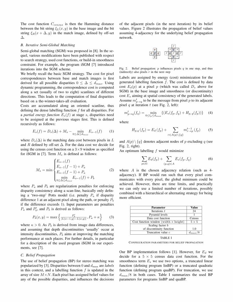
of the adjacent pixels (in the next iteration) by its beliefvalues. Figure 2 illustrates the propagation of belief valuesassuming 4-adjacency for the underlying belief propagationnetwork.

Fig. 2. Belief propagation: p influences pixels q in one step, and thus(indirectly) also pixels r in the next step

Labels are assigned by energy (cost) minimization for thegenerated labelling function f . The cost is defined by datacost Ed(p) at a pixel p (which was called Ds above forSGM) in the base image and smoothness (or discontinuity)cost Es aiming at spatial consistency of the generated labels.Assume mt

p→q to be the message from pixel p to its adjacentpixel q at iteration t (see Fig. 2, left):

mtp→q(fq) = min

0≤lp≤dmax

(Es(fp, fq) +Hp, q(fp)) (4)

where

Hp,q (fp) = Ed (fp) +∑

r∈A(p)\q

mt−1r→p (fp) (5)

and A(p)\q denotes adjacent nodes of p excluding q (seeFig. 2, right).An optimum labelling f would minimize∑

p∈Ω

Ed(fp) +∑

(p,q)∈A

Es(fp, fq) (6)

where A is the chosen adjacency relation (such as 4-adjacency). If BP would run such that every pixel com-municates with every pixel, the global minimum could beachieved. However, there are time limits, and practicallywe can only use a limited number of iterations, possiblycombined with a hierarchical or alternating strategy for beingmore efficient.

Parameter ValueIterations t 24

Pyramid levels 1Data cost function Census

Cost function window (width× height) 5× 5Scaling factor b

of discontinuity function 1.0Truncation value c dmax/8

TABLE ICONFIGURATION PARAMETERS FOR BELIEF PROPAGATION

Our BP implementation follows [1]. However, for Ed wedecide for a 5 × 5 census data cost function. For thesmoothness term Es we use two options, a truncated linearfunction (defining program linBP) or a truncated quadraticfunction (defining program quaBP). For truncation, we usedmax/8 in both cases. Table I summarizes the used BPparameters for programs linBP and quaBP.

III. VIDEO SEQUENCES WITH GROUND TRUTH

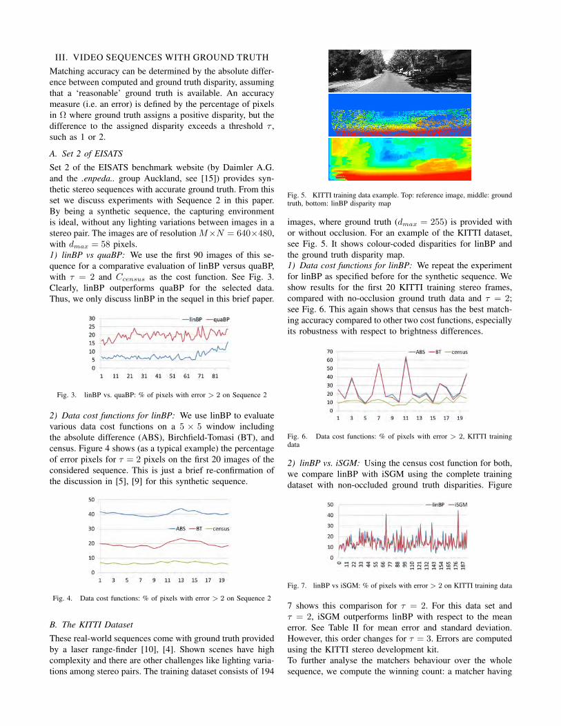
Matching accuracy can be determined by the absolute differ-ence between computed and ground truth disparity, assumingthat a ‘reasonable’ ground truth is available. An accuracymeasure (i.e. an error) is defined by the percentage of pixelsin Ω where ground truth assigns a positive disparity, but thedifference to the assigned disparity exceeds a threshold τ ,such as 1 or 2.

A. Set 2 of EISATS

Set 2 of the EISATS benchmark website (by Daimler A.G.and the .enpeda.. group Auckland, see [15]) provides syn-thetic stereo sequences with accurate ground truth. From thisset we discuss experiments with Sequence 2 in this paper.By being a synthetic sequence, the capturing environmentis ideal, without any lighting variations between images in astereo pair. The images are of resolution M×N = 640×480,with dmax = 58 pixels.1) linBP vs quaBP: We use the first 90 images of this se-quence for a comparative evaluation of linBP versus quaBP,with τ = 2 and Ccensus as the cost function. See Fig. 3.Clearly, linBP outperforms quaBP for the selected data.Thus, we only discuss linBP in the sequel in this brief paper.

Fig. 3. linBP vs. quaBP: % of pixels with error > 2 on Sequence 2

2) Data cost functions for linBP: We use linBP to evaluatevarious data cost functions on a 5 × 5 window includingthe absolute difference (ABS), Birchfield-Tomasi (BT), andcensus. Figure 4 shows (as a typical example) the percentageof error pixels for τ = 2 pixels on the first 20 images of theconsidered sequence. This is just a brief re-confirmation ofthe discussion in [5], [9] for this synthetic sequence.

Fig. 4. Data cost functions: % of pixels with error > 2 on Sequence 2

B. The KITTI Dataset

These real-world sequences come with ground truth providedby a laser range-finder [10], [4]. Shown scenes have highcomplexity and there are other challenges like lighting varia-tions among stereo pairs. The training dataset consists of 194

Fig. 5. KITTI training data example. Top: reference image, middle: groundtruth, bottom: linBP disparity map

images, where ground truth (dmax = 255) is provided withor without occlusion. For an example of the KITTI dataset,see Fig. 5. It shows colour-coded disparities for linBP andthe ground truth disparity map.1) Data cost functions for linBP: We repeat the experimentfor linBP as specified before for the synthetic sequence. Weshow results for the first 20 KITTI training stereo frames,compared with no-occlusion ground truth data and τ = 2;see Fig. 6. This again shows that census has the best match-ing accuracy compared to other two cost functions, especiallyits robustness with respect to brightness differences.

Fig. 6. Data cost functions: % of pixels with error > 2, KITTI trainingdata

2) linBP vs. iSGM: Using the census cost function for both,we compare linBP with iSGM using the complete trainingdataset with non-occluded ground truth disparities. Figure

Fig. 7. linBP vs iSGM: % of pixels with error > 2 on KITTI training data

7 shows this comparison for τ = 2. For this data set andτ = 2, iSGM outperforms linBP with respect to the meanerror. See Table II for mean error and standard deviation.However, this order changes for τ = 3. Errors are computedusing the KITTI stereo development kit.To further analyse the matchers behaviour over the wholesequence, we compute the winning count: a matcher having

Mean (%) Standard deviation (%)iSGM linBP iSGM linBP

2 pixel 12.22 12.45 5.23 6.023 pixel 9.40 9.23 4.41 5.14

TABLE IILINBP VS ISGM: COMPLETE KITTI TRAINING DATASET

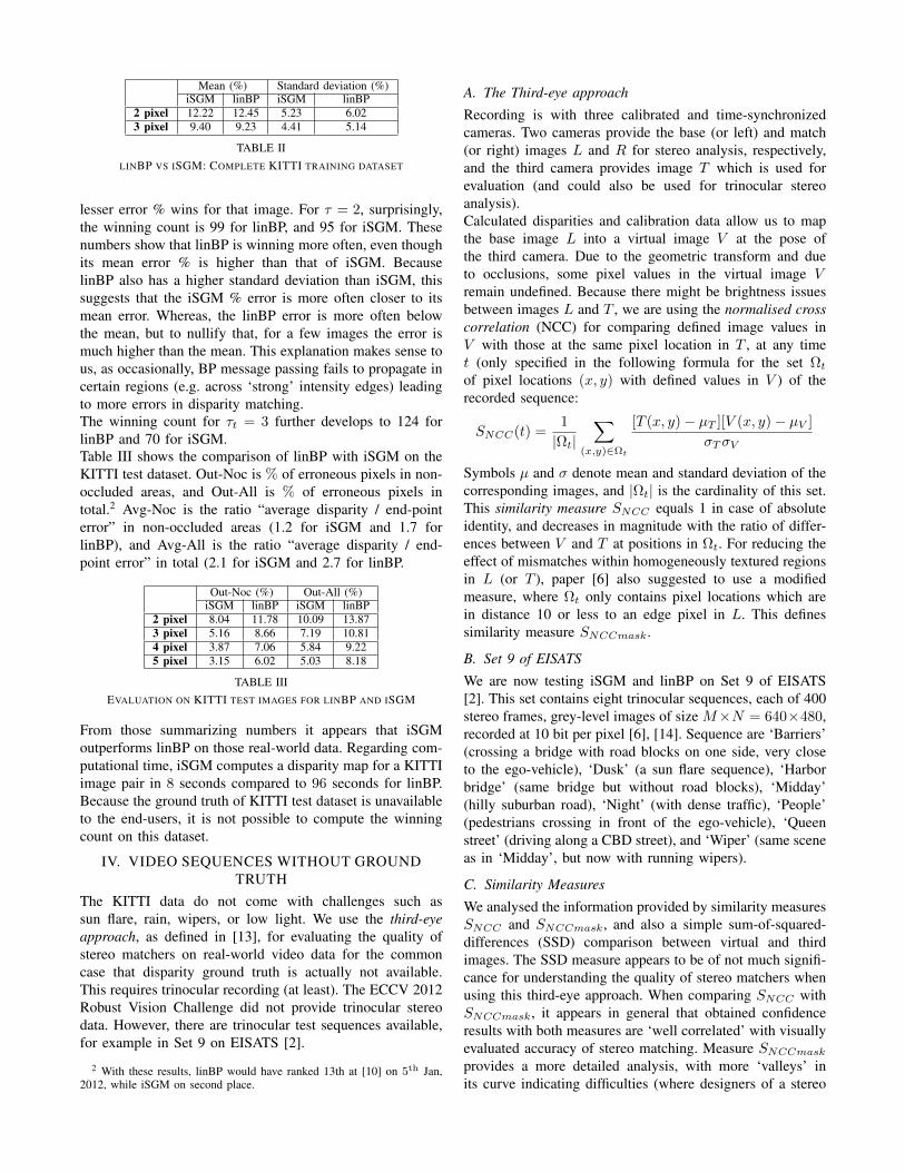
lesser error % wins for that image. For τ = 2, surprisingly,the winning count is 99 for linBP, and 95 for iSGM. Thesenumbers show that linBP is winning more often, even thoughits mean error % is higher than that of iSGM. BecauselinBP also has a higher standard deviation than iSGM, thissuggests that the iSGM % error is more often closer to itsmean error. Whereas, the linBP error is more often belowthe mean, but to nullify that, for a few images the error ismuch higher than the mean. This explanation makes sense tous, as occasionally, BP message passing fails to propagate incertain regions (e.g. across ‘strong’ intensity edges) leadingto more errors in disparity matching.The winning count for τt = 3 further develops to 124 forlinBP and 70 for iSGM.Table III shows the comparison of linBP with iSGM on theKITTI test dataset. Out-Noc is % of erroneous pixels in non-occluded areas, and Out-All is % of erroneous pixels intotal.2 Avg-Noc is the ratio “average disparity / end-pointerror” in non-occluded areas (1.2 for iSGM and 1.7 forlinBP), and Avg-All is the ratio “average disparity / end-point error” in total (2.1 for iSGM and 2.7 for linBP.

Out-Noc (%) Out-All (%)iSGM linBP iSGM linBP

2 pixel 8.04 11.78 10.09 13.873 pixel 5.16 8.66 7.19 10.814 pixel 3.87 7.06 5.84 9.225 pixel 3.15 6.02 5.03 8.18

TABLE IIIEVALUATION ON KITTI TEST IMAGES FOR LINBP AND ISGM

From those summarizing numbers it appears that iSGMoutperforms linBP on those real-world data. Regarding com-putational time, iSGM computes a disparity map for a KITTIimage pair in 8 seconds compared to 96 seconds for linBP.Because the ground truth of KITTI test dataset is unavailableto the end-users, it is not possible to compute the winningcount on this dataset.

IV. VIDEO SEQUENCES WITHOUT GROUNDTRUTH

The KITTI data do not come with challenges such assun flare, rain, wipers, or low light. We use the third-eyeapproach, as defined in [13], for evaluating the quality ofstereo matchers on real-world video data for the commoncase that disparity ground truth is actually not available.This requires trinocular recording (at least). The ECCV 2012Robust Vision Challenge did not provide trinocular stereodata. However, there are trinocular test sequences available,for example in Set 9 on EISATS [2].

2 With these results, linBP would have ranked 13th at [10] on 5th Jan,2012, while iSGM on second place.

A. The Third-eye approach

Recording is with three calibrated and time-synchronizedcameras. Two cameras provide the base (or left) and match(or right) images L and R for stereo analysis, respectively,and the third camera provides image T which is used forevaluation (and could also be used for trinocular stereoanalysis).Calculated disparities and calibration data allow us to mapthe base image L into a virtual image V at the pose ofthe third camera. Due to the geometric transform and dueto occlusions, some pixel values in the virtual image Vremain undefined. Because there might be brightness issuesbetween images L and T , we are using the normalised crosscorrelation (NCC) for comparing defined image values inV with those at the same pixel location in T , at any timet (only specified in the following formula for the set Ωt

of pixel locations (x, y) with defined values in V ) of therecorded sequence:

SNCC(t) =1

|Ωt|∑

(x,y)∈Ωt

[T (x, y)− µT ][V (x, y)− µV ]

σTσV

Symbols µ and σ denote mean and standard deviation of thecorresponding images, and |Ωt| is the cardinality of this set.This similarity measure SNCC equals 1 in case of absoluteidentity, and decreases in magnitude with the ratio of differ-ences between V and T at positions in Ωt. For reducing theeffect of mismatches within homogeneously textured regionsin L (or T ), paper [6] also suggested to use a modifiedmeasure, where Ωt only contains pixel locations which arein distance 10 or less to an edge pixel in L. This definessimilarity measure SNCCmask.

B. Set 9 of EISATS

We are now testing iSGM and linBP on Set 9 of EISATS[2]. This set contains eight trinocular sequences, each of 400stereo frames, grey-level images of size M×N = 640×480,recorded at 10 bit per pixel [6], [14]. Sequence are ‘Barriers’(crossing a bridge with road blocks on one side, very closeto the ego-vehicle), ‘Dusk’ (a sun flare sequence), ‘Harborbridge’ (same bridge but without road blocks), ‘Midday’(hilly suburban road), ‘Night’ (with dense traffic), ‘People’(pedestrians crossing in front of the ego-vehicle), ‘Queenstreet’ (driving along a CBD street), and ‘Wiper’ (same sceneas in ‘Midday’, but now with running wipers).

C. Similarity Measures

We analysed the information provided by similarity measuresSNCC and SNCCmask, and also a simple sum-of-squared-differences (SSD) comparison between virtual and thirdimages. The SSD measure appears to be of not much signifi-cance for understanding the quality of stereo matchers whenusing this third-eye approach. When comparing SNCC withSNCCmask, it appears in general that obtained confidenceresults with both measures are ‘well correlated’ with visuallyevaluated accuracy of stereo matching. Measure SNCCmask

provides a more detailed analysis, with more ‘valleys’ inits curve indicating difficulties (where designers of a stereo

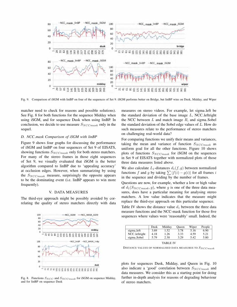
Fig. 9. Comparison of iSGM with linBP on four of the sequences of Set 9. iSGM performs better on Bridge, but linBP wins on Dusk, Midday, and Wiper

matcher need to check for reasons and possible solutions).See Fig. 8 for both functions for the sequence Midday whenusing iSGM, and for sequence Dusk when using linBP. Inconclusion, we decide to use measure SNCCmask only in thesequel.

D. NCC mask Comparison of iSGM with linBP

Figure 9 shows four graphs for discussing the performanceof iSGM and linBP on four sequences of Set 9 of EISATS,showing functions SNCCmask only for both stereo matchers.For many of the stereo frames in those eight sequencesof Set 9, we visually evaluated that iSGM is the betteralgorithm compared to linBP due to ‘appealing accuracy’at occlusion edges. However, when summarizing by usingthe SNCCmask measure, surprisingly the opposite appearsto be the dominating event (i.e. linBP appears to win morefrequently).

V. DATA MEASURES

The third-eye approach might be possibly avoided by cor-relating the quality of stereo matchers directly with data

Fig. 8. Functions SNCC and SNCCmask for iSGM on sequence Midday,and for linBP on sequence Dusk

measures on stereo videos. For example, let sigma left bethe standard deviation of the base image L, NCC leftrightthe NCC between L and match image R, and sigma Sobelthe standard deviation of the Sobel edge values of L. How dosuch measures relate to the performance of stereo matcherson challenging real-world data?For comparing functions we unify their means and variances,taking the mean and variance of function SNCCmask asuniform goal for all the other functions. Figure 10 showsplots of functions SNCCmask for iSGM on the sequencesin Set 9 of EISATS together with normalized plots of thosethree data measures listed above.We also calculate L1-distances d1(f, g) between normalizedfunctions f and g by taking

∑|f(i)− g(i)| for all frames i

in the sequence and dividing by the number of frames.Questions are now, for example, whether a low or high valueof d1(SNCCmask, g), where g is one of the three data mea-sures, does have a particular meaning for analysing stereomatchers. A low value indicates that the measure mightreplace the third-eye approach on this particular sequence.Table IV shows the distance value d1 between the three datameasure functions and the NCC-mask function for those fivesequences where values were ‘reasonably’ small. Indeed, the

Dusk Midday Queen Wiper Peoplesigma left 3.69 1.52 3.78 5.16 6.90NCC leftright 4.18 1.26 3.33 4.59 5.21sigma Sobel 5.79 2.30 3.29 5.42 5.80

TABLE IVDISTANCE VALUES OF NORMALISED DATA MEASURES TO SNCCmask

plots for sequences Dusk, Midday, and Queen in Fig. 10also indicate a ‘good’ correlation between SNCCmask anddata measures. We consider this as a starting point for doingfurther in-depth analysis for reasons of degrading behaviourof stereo matchers.

Fig. 10. Comparison of NCC mask of iSGM on Set 9 of EISATS with NCC mask-normalized functions sigma left, NCC leftright, and sigma Sobel

VI. CONCLUSIONSThe results came partially as a surprise to us. However,there is also a good logic behind. BP is propagating beliefsequentially row-wise with feedback from adjacent rows,without paying particular attention to vertical propagationsor accuracy along horizontal disparity discontinuities, asiSGM does. Thus, iSGM outperforms BP at disparity dis-continuities. However, depth accuracy within object regionsappears to be better with linBP. In the sequence Bridgewe do have many structural details and not such a highratio of homogeneous regions - accordingly, iSGM is win-ning here. In the Wiper sequence, the NCC leftright datameasure indicates correctly the actual input data situation,corresponds to the performance of the stereo matchers, andBP is able to cope better with those data (see also [14]). Itwould be of benefit to have trinocular data with ground truthfor challenging situations, allowing to correlate ground truth,similarity measures, and data measures more in detail. Theproposed approach helps to identify critical events for stereomatchers which need to be resolved in future.

ACKNOWLEDGMENT

The authors thank Simon Hermann for providing programiSGM for the performed experiments and discussions whilewriting the paper. The authors also thank Sandino Moralesfor providing his sources for the third-eye approach.

REFERENCES

[1] C. C. Cheng, C. K. Liang, Y. C. Lai, H. H. Chen, and L. G. Chen. Fastbelief propagation process element for high-quality stereo estimation.In Proc. IEEE Int. Conf. on Acoustics, Speech, and Signal Processing,pages 745–748, 2009.

[2] EISATS benchmark data base. The University of Auckland, www.mi.auckland.ac.nz/EISATS, 2013.

[3] P. F. Felzenszwalb and D. P. Huttenlocher. Efficient belief propagationfor early vision. Int. J. Computer Vision, volume 70, pages 41–54,2006.

[4] A. Geiger, P. Lenz, and R. Urtasun. Are we ready for autonomousdriving? The KITTI Vision Benchmark Suite. In Proc. IEEE Int. Conf.Computer Vision Pattern Recognition, pages 3354–3361, 2012.

[5] S. Hermann, and R. Klette. The naked truth about cost func-tions for stereo matching. MI-tech report 33, The Univer-sity of Auckland, www.mi.auckland.ac.nz/tech-reports/MItech-TR-33.pdf, 2009.

[6] S. Hermann, S. Morales, and R. Klette. Half-resolution semi-globalstereo matching. In Proc. IEEE Intelligent Vehicles Symposium, pages201–206, 2011.

[7] S. Hermann and R. Klette. Iterative semi-global matching for robustdriver assistance systems. In Proc. Asian Conf. Computer Vision,LNCS, 2012.

[8] H. Hirschmuller. Accurate and efficient stereo processing by semi-global matching and mutual information. In Proc. IEEE Int. Conf.Computer Vision Pattern Recognition, volume 2, page 807–814, 2005.

[9] H. Hirschmuller and D. Scharstein. Evaluation of stereo matching costson images with radiometric differences. IEEE Trans. Pattern AnalysisMachine Intelligence, volume 31, pages 1582–1599, 2009.

[10] KITTI vision benchmark suite. Karlsruhe Institute of Technology,www.cvlibs.net/datasets/kitti/, 2013.

[11] R. Klette, N. Kruger, T. Vaudrey, K. Pauwels, M. Hulle, S. Morales,F. Kandil, R. Haeusler, N. Pugeault, C. Rabe and M. Lappe. Perfor-mance of correspondence algorithms in vision-based driver assistanceusing an online image sequence database. IEEE Trans. VehicularTechnology, volume 60, pages 2012–2026, 2011.

[12] D. Kondermann and W. Niehsen. 2012 robust vision challenge.hci.iwr.uni-heidelberg.de/Static/challenge2012/RVC2012_Results.pdf, 2012.

[13] S. Morales and R. Klette. A third eye for performance evaluation instereo sequence analysis. In Proc. Int. Conf. Computer Analysis ImagesPatterns, pages 1078–1086, 2009.

[14] K. Schauwecker, S. Morales, S. Hermann, and R. Klette. A compar-ative study of stereo-matching algorithms for road-modeling in thepresence of windscreen wipers. In Proc. IEEE Intelligent VehiclesSymposium, pages 7–12, 2011.

[15] T. Vaudrey, C. Rabe, R. Klette, and J. Milburn. Differences betweenstereo and motion behaviour on synthetic and real-world stereo se-quences. In Proc. Int. Conf. Image Vision Computing New Zealand,pages 1-6, 2008.

[16] R. Zabih, and J. Woodfill. Non-parametric local transforms for com-puting visual correspondence. In Proc. IEEE Int. European Conf.Computer Vision, pages 151–158, 1994.