Fast Bilateral-Space Stereo

Ugo Capeto∗

January 19, 2017

1 Introduction

In my never ending search for the ”perfect” stereo matching algorithm, I came across Barronet al.’s paper ”Fast Bilateral-Space Stereo for Synthetic Defocus” [1] and was quite impressedby a sample depth map Barron et al. are showing in that paper (reproduced in Figure 1).

Figure 1: Sample depth map obtained by Barron et al. On the left is the left image of astereo pair, on the right is the depth map.

This depth map has well-defined edges that match the edges of the left image. This is inmy opinion crucial although it is often overlooked in the literature when the time comes tojudge the depth maps quality. There are areas where the disparity is wrong but because theyare well smoothed out, they do not stick out too much (They can still be problematic howeverdepending on the application.) Areas where the disparity is wrong are usually unavoidableif there is no texture or the texture is repeated. In any case, this depth map looks quitegood. In the following, I go through the method described by Barron et al. and show somedepth maps obtained by the method (using my own implementation).

∗e-mail: ugocapetodifrancia3d@gmail.com

1

2 Fast Bilateral-Space Stereo

Barron et al. use a global approach to generate the depth map, that is, they are trying tominimize a cost function where the unknowns are the pixel disparities:

mindi

(1

2

∑i

∑j

Ai,j(di − dj)2 + λ∑i

fi(di)) (1)

Ai,j is the bistochastic version (all rows and columns add up to 1) of the bilateral filterAi,j:

Ai,j = exp(−‖(xi, yi)− (xj, yj‖2

2σ2xy

− ‖(ri, gi, bi)− (rj, gj, bj‖2

2σ2rgb

) (2)

Where σxy and σrgb control the bandwidth in the two-dimensional pixel space (x, y) andthe three-dimensional color space (r, g, b) of the image, respectively.

The value of Ai,j decreases (from 1) as pixel j defined by coordinates (xj, yj) in pixelspace and color intensities (rj, gj, bj) in color space gets further away in either the pixelspace or the color space from pixel i defined by coordinates (xi, yi) in pixel space and colorintensities (ri, gi, bi) in color space.

Going back to equation 1, if pixel j is similar in color to pixel i and is close to pixel i inspace, Ai,j will be close to 1 and if the disparities di, dj are different, the smoothness term

Ai,j(di − dj)2 will carry a penalty. This is a desired behaviour because two pixels close toeach other and of similar color should really be at the same depth unless there is a depthchange without a change of color. If pixel j is dissimilar in color to pixel i, even if it isclose to pixel i in space, Ai,j will be small and even if the disparities di, dj are different, thepenalty will be small. This is another desired behaviour because even though a color changedoesn’t always mean a depth change, a depth change almost always means a color change.In other words, a color change should not penalize a disparity change.

The bilateral filter is typically used to smooth an image while preserving its edges. Foreach pixel i of an image, one would typically consider a square (kernel) centered at i andperform a convolution using Ai,j as the convolution weight. Note that this can get expensiverather quickly as the image size grows and/or the extent of the convolution (the size of thekernel) increases.

It is not the first time the bilateral filter is used in stereo matching [5] but it appears tobe the first time it is used in the smoothness term of the cost function of a global method.Usually, the smoothness term of a cost function only involves the nearest neighboring pixelsand takes one of two values: a small value if the colors are dissimilar in order not to penalizea depth change or a larger value if the colors are similar in order to penalize a depth change.In other words, the smoothness term is usually quite simplistic.

The function fi(di) in equation 1 is the data matching cost for pixel i, in other words,it gives the matching cost as a function of the disparity di. Given pixel i in the left imagedefined by the coordinates (xi, yi), the corresponding pixel in the right image for the disparitydi has coordinates (xi−di, yi) as the stereo pair is assumed to be rectified. The data matchingcost is low if the colors of pixel i and its corresponding pixel are similar or high (to a point if

2

truncation is used) if the colors are dissimilar. Barron et al. use a data matching cost basedon the Birchfield-Tomasi criterio which is described next.

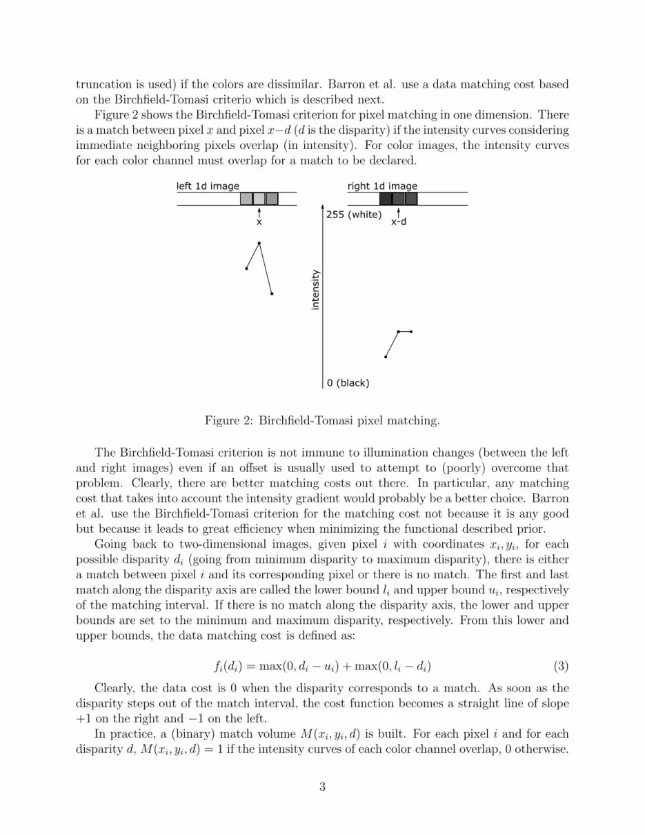
Figure 2 shows the Birchfield-Tomasi criterion for pixel matching in one dimension. Thereis a match between pixel x and pixel x−d (d is the disparity) if the intensity curves consideringimmediate neighboring pixels overlap (in intensity). For color images, the intensity curvesfor each color channel must overlap for a match to be declared.

inte

nsity

0 (black)

255 (white)x x-d

left 1d image right 1d image

Figure 2: Birchfield-Tomasi pixel matching.

The Birchfield-Tomasi criterion is not immune to illumination changes (between the leftand right images) even if an offset is usually used to attempt to (poorly) overcome thatproblem. Clearly, there are better matching costs out there. In particular, any matchingcost that takes into account the intensity gradient would probably be a better choice. Barronet al. use the Birchfield-Tomasi criterion for the matching cost not because it is any goodbut because it leads to great efficiency when minimizing the functional described prior.

Going back to two-dimensional images, given pixel i with coordinates xi, yi, for eachpossible disparity di (going from minimum disparity to maximum disparity), there is eithera match between pixel i and its corresponding pixel or there is no match. The first and lastmatch along the disparity axis are called the lower bound li and upper bound ui, respectivelyof the matching interval. If there is no match along the disparity axis, the lower and upperbounds are set to the minimum and maximum disparity, respectively. From this lower andupper bounds, the data matching cost is defined as:

fi(di) = max(0, di − ui) + max(0, li − di) (3)

Clearly, the data cost is 0 when the disparity corresponds to a match. As soon as thedisparity steps out of the match interval, the cost function becomes a straight line of slope+1 on the right and −1 on the left.

In practice, a (binary) match volume M(xi, yi, d) is built. For each pixel i and for eachdisparity d, M(xi, yi, d) = 1 if the intensity curves of each color channel overlap, 0 otherwise.

3

For each pixel i, the lower and upper bounds of the matching interval (li and ui) are obtainedby scanning through M(xi, yi, d) along d. Relying on pixel to pixel matches for the data costis prone to inacurracies for various reasons, therefore patch to patch matches are preferred.One can switch from pixel to pixel matches to patch to patch matches by applying an ”and”filter to each ”slice” d of the match volume prior to getting the lower and upper bounds of thematching interval for each pixel. Applying an ”and” filter to a ”slice” d of the match volumeis equivalent to requiring that, for a given pixel i, all pixels in the square patch centeredat i must record a match, not just pixel i. Clearly, this improves matching accuracy in theinterior of objects, but not on the boundary of objects where the background usually differbetween the left and right images. In other words, for pixels at or near object boundaries,no match will be recorded along the disparity axis and the data matching cost will be 0and not be a factor in the solution. Indeed, the smoothness term is likely to take over anddictate what the disparity is supposed to be by ”propagating” the disparity in the interiorof the object. This is fine for objects large enough that matches are properly made in theirinteriors, but it is a problem for objects that are thin along the width of the image. If theimage has thin objects and the patch size is too large, these thin structures will not showup in the depth map.

The factor λ in front of the data matching cost fi(di) is there so that one can balance asbest as possible the smoothness cost and the data cost.

Trying to solve equation 1 would probably be extremely slow for average size pictures.Large speed improvements can be obtained by ”splatting” the problem into a higher-dimensionalbilateral space. For a two dimensional image, the bilateral space has five dimensions: two for(x, y) (coordinates in the image plane) and three for (r, g, b) (three color channels). Figure 3shows a bilateral space grid for a one-dimensional grayscale image. This bilateral space gridconcept was first introduced in [2] in order to speed up bilateral filtering.

The idea is to, instead of applying a bilateral filter in pixel space, (1) ”splat” the pixelsaccording to their location and color into a five-dimensional bilateral grid, (2) blur the gridusing a short range isotropic blur filter, and (3) ”slice” the grid in order to recover the filteredimage. The size of the grid cells in the (x, y) directions (referred to as the sampling rate ofthe spatial axes ss) kinda determines how much smoothing is performed. The size of the gridcells in the (r, g, b) directions kinda determines how much the edges are preserved (referredto as the sampling rate of the range axes sr).

Going back to Figure 3, the one-dimensional edge is clearly dark left of center and clearlylight right of center. A bilateral filter would smooth the colors on either side of the centerand keep the intensities separated (the darks would remain dark and the lights would remainlight, only smoother). Now, if you consider a 3x3 blur filter and apply it to the grid, the gridcells containing the dark pixels are not affected by the grid cells containing the light pixels,and therefore the filtered image will still have its center separating the darks and the lights.

Instead of solving equation 1 in pixel space, Barron et al. propose to solve:

min~v

(~vT (Cs − CnBCn)~v + λ∑j

gj(vj)) (4)

It takes quite a bit of mathematical manipulation to go from equation 1 to equation 4 andso, the interested reader is invited to go over Barron et al.’s paper as well as the supplemental

4

x

inte

nsity

1d image

bilateral space grid

Figure 3: Bilateral space grid.

material to fully understand how equation 4 is derived.For any grid cell containing at least one pixel, a bilateral space vertex j is created. The

vector ~v is the vector of the unknown disparities vj of the vertices. The matrix B is the”blur” matrix defined as the sum of ”blur” matrices in each bilateral space direction (each”blur” matrix corresponds to a narrow [1, 2, 1] ”blur” kernel). The matrix Cs is a diagonalmatrix where each diagonal entry is the ”mass” of the corresponding vertex, which is thenumber of pixels contained in the vertex. The matrix Cn is such that (CnBCn)~1 = Cs

~1.The data cost at the vertex level gj(vj) is computed by summing the data cost of the pixelscontained in the vertex j using disparity vj for the pixel.

Equation 4 which is an unconstrained minimization problem can be solved efficiently withL-BFGS. To use L-BFGS, we need to be able to evaluate the bilateral space cost functionand its gradient as well. Because vj may not be an integer during the L-BFGS iterations,gj(vj) has to be interpolated (linearly) between bvjc (floor) and dvje (ceiling):

gj(vj) = (dvje − vj)gj(bvjc) + (vj − bvjc)gj(dvje) (5)

The gradient of the bilateral space cost function is defined analytically as:

∇cost(~v) = 2(Cs − CnBCn)~v + λ[g1(dv1e)− g1(bv1c); . . . ; gM(dvMe)− gM(bvMc)] (6)

Where M is the number of bilateral space vertices. Once L-BFGS has converged, thedisparity at the vertex level is transferred back (”sliced”) to the pixels it contains. This

5

transfer may lead to ”blocky” depth maps. Barron et al. use a domain transform filter [3]to smooth out the blocky artifacts.

In order to improve the speed of their algorithm, Barron et al. construct a pyramid ofbilateral representations and solve equation 4 in each bilateral representation going fromcoarse to fine. Although it is clear that a pyramid of bilateral representations improves theconvergence of L-BFGS, it is not clear whether it has a positive impact on the quality ofthe depth maps generated. It would certainly seem that using a coarse to fine bilateralrepresentation may increase the reach of the ”blur” filter and make smoothing less localized.

3 Results

In order to properly assess the quality of the depth maps produced by Barron et al.’s method,it needs to be implemented. My version does not use multiscale optimization, does notsmooth the depth maps with the edge-preserving domain transform, and is probably quitenaive. Other than that, I believe that my implementation is quite faithful to Barron et al.’spaper and the likelihood of a bug is remote albeit possible. The L-BFGS software I usecomes from [4].

I tested my implementation of Fast Bilateral-Space Stereo on seleted stereo pairs from theMiddlebury stereo image database, namely, Art, Books, Dolls, Motorcycle, and Playroom.Note that the Middlebury stereo pairs do not suffer from illumination changes which makesthe Birchfield-Tomasi criterion for matching cost not a terrible idea after all.

For the Art dataset (Figure 4), the parameters were: minimum disparity 26, maximumdisparity 72, ss = 8, sr = 16, patch radius 4, and λ = 0.1.

Figure 4: Left image and depth map (obtained with my own implementation of Fast Bilateral-Space Stereo) for the Art dataset.

For the Books dataset (Figure 4), the parameters were: minimum disparity 24, maximumdisparity 73, ss = 8, sr = 32, patch radius 7, and λ = 0.1.

For the Dolls dataset (Figure 4), the parameters were: minimum disparity 22, maximumdisparity 70, ss = 8, sr = 32, patch radius 4, and λ = 0.1.

6

Figure 5: Left image and depth map (obtained with my own implementation of Fast Bilateral-Space Stereo) for the Books dataset.

For the Motorcycle dataset (Figure 7), the parameters were: minimum disparity 0, max-imum disparity 270, ss = 8, sr = 32, patch radius 12, and λ = 0.1.

For the Playroom dataset (Figure 7), the parameters were: minimum disparity 0, maxi-mum disparity 330, ss = 8, sr = 32, patch radius 12, and λ = 0.1.

The quality of the depth maps produced by Fast Bilateral Space Stereo is in general quitegood but there are definitely problems. What is really striking is that, as disparities/depthsare propagated along areas of similar color, you end up with rather large areas (of similarcolor) at the (very) wrong depth. To me, this is the main issue.

4 Conclusion

Because Fast Bilateral Space Stereo uses the bilateral filter in a reduced space called thebilateral space, it is fast. However, the data matching cost that is used (for efficiencypurposes) is relatively poor. This leads to over-smoothing in an effort to reduce the effectsof the not-so-great data matching cost. This over-smoothing may produce large areas ofsimilar colors at the wrong depth, which may or may not be a problem depending upon theapplication. It should be noted that Fast Bilateral Space Stereo does not explicitly handleocclusions but it seems that bilateral filter smoothing/blurring kinda takes care of that.

References

[1] Jonathan T Barron, Andrew Adams, YiChang Shih, and Carlos Hernandez. Fastbilateral-space stereo for synthetic defocus. In Proceedings of the IEEE Conference onComputer Vision and Pattern Recognition, pages 4466–4474, 2015.

7

Figure 6: Left image and depth map (obtained with my own implementation of Fast Bilateral-Space Stereo) for the Dolls dataset.

Figure 7: Left image and depth map (obtained with my own implementation of Fast Bilateral-Space Stereo) for the Motorcycle dataset.

[2] Jiawen Chen, Sylvain Paris, and Fredo Durand. Real-time edge-aware image processingwith the bilateral grid. In ACM Transactions on Graphics (TOG), volume 26, page 103.ACM, 2007.

[3] Eduardo SL Gastal and Manuel M Oliveira. Domain transform for edge-aware image andvideo processing. In ACM Transactions on Graphics (TOG), volume 30, page 69. ACM,2011.

[4] Naoaki Okazaki. liblbfgs: a library of limited-memory broyden-fletcher-goldfarb-shanno(l-bfgs). http://www.chokkan.org/software/liblbfgs/. Accessed June 15, 2015.

[5] Kuk-Jin Yoon and In So Kweon. Adaptive support-weight approach for correspondencesearch. 2006.

8

Figure 8: Left image and depth map (obtained with my own implementation of Fast Bilateral-Space Stereo) for the Playroom dataset.

9