Stereo vision for autonomous ferry
176
NTNU Norwegian University of Science and Technology Faculty of Information Technology and Electrical Engineering Department of Engineering Cybernetics Master’s thesis Lina Charlotte Kristoffersen Theimann Trine Ødegård Olsen Stereo vision for autonomous ferry Master’s thesis in Cybernetics and Robotics Supervisor: Edmund Førland Brekke, Co-supervisor: Annette Stahl, Øystein K. Helgesen. June 2020
-
Upload
khangminh22 -
Category
Documents
-
view
6 -
download
0
Transcript of Stereo vision for autonomous ferry

NTN
UN
orw
egia
n U
nive
rsity
of S
cien
ce a
nd T
echn
olog
yFa
culty
of I
nfor
mat
ion
Tech
nolo
gy a
nd E
lect
rical
Engi
neer
ing
Dep
artm
ent o
f Eng
inee
ring
Cybe
rnet
ics
Mas
ter’s
thes
is
Lina Charlotte Kristoffersen TheimannTrine Ødegård Olsen
Stereo vision for autonomous ferry
Master’s thesis in Cybernetics and Robotics
Supervisor: Edmund Førland Brekke,
Co-supervisor: Annette Stahl, Øystein K. Helgesen.
June 2020

Lina Charlotte Kristoffersen TheimannTrine Ødegård Olsen
Stereo vision for autonomous ferry
Master’s thesis in Cybernetics and RoboticsSupervisor: Edmund Førland Brekke,Co-supervisor: Annette Stahl, Øystein K. Helgesen.June 2020
Norwegian University of Science and TechnologyFaculty of Information Technology and Electrical EngineeringDepartment of Engineering Cybernetics

Abstract
The thesis discusses far-range object detection for stereo, calibration, and system imple-mentation for unmanned surface vehicles. The stereo system record with a baseline of 1.80meters, with a fixation point at 50 meters. For far range distance estimation, a procedurefor extrinsic stereo calibration is introduced. Testing the procedure at different distances,show that the selected scene is of higher importance than calibrating at the operating range.The calibration at 20 meters achieves the best overall distance estimates.
The stereo system is designed for the autonomous ferry milliAmpere, and tested in a mar-itime environment. The system processes raw sensor data and output world coordinatesof the detected objects. The disparity map created using Sum of Absolute Difference(SAD) and a Fast Global Image Smoothing based on Weighted Least Square (WLS) filter,is robust and has low computational cost. For object detection purposes, two clusteringtechniques are implemented. A convolution neural network is applied for classification,and used in combination with the disparity map to extract 3D positions of objects. Themethod is robust against noise in the disparity map, but appear to be partially inconsistentin the estimates. An alternative detection method based on hierarchical clustering usingEuclidean distance yields more reliable detections, but is more prone to noise. The imple-mented system shows potential for vessel detection in a range of 10 to 200 meters, but it isstill not clear that the detection performance is good enough to rely on in an autonomouscollision avoidance system.
i
Sammendrag
Denne oppgaven diskuterer stereosyn for a detetktere objekter pa lange distanser, kali-brering og system implementasjon for et førerløst fartøy. Oppsettet innehar en interaksiellavstand pa 1.80 meter mellom kameraene for a optimalt detektere objekter pa 50 metersavstand. En metode for a kalibrere pa lengre avstander er foreslatt. Metoden er testet ogresultatene viser at valg av kalibrerings scene er viktigere enn avstanden til kalibrering-sobjektet. Kalibreringen utført pa 20 meter viste a gi mest nøyaktige dybdeestimat.
Systemet er designet for fergen milliAmpere og er testet i et marint miljø. Systemet pros-esserer ra sensordata og gir ut verdenskoordinater til detekterte objekter. Dybdekartet erimplementert ved bruk av algoritmene Sum of Absolute Differences og Fast Global ImageSmoothing filter basert pa minste kvadraters metode viser seg a være robust. To metoderer implementert for a detektere objekter i dybdekartet. Ett konvolusjonelt nevralt nettverk(CNN) for klassifisering gir i kombinasjon med dybdekartet verdensposisjonen til objekterav interesse. Metoden viser seg a være robust mot støy, men har noe inkonsekvente esti-mater. En alernativ metode deteksjonsmetode basert pa hierarkisk grupperingsalgoritmesom bruker Euklidsk avstand gir mer palitelige deteksjoner, men er mer utsatt for støy idybdekartet. Det implementerte systemet viser potensiale for a detektere objekter i avs-tander mellom 10 og 200 meter, men ytterligere testing ma utføres for a kunne integreresensoren i ett helhetlig system for navigasjon av et autonomt fartøy.
ii
Preface
This is the concluding part of a 5-year Masters’s degree in Cybernetics and Robotics atthe Norwegian University of Science and Technology (NTNU). We want to thank our su-pervisor Edmund Førland Brekke for valuable feedback, guidance, and support during thisthesis. Also, we would like to thank our two co-supervisors Annette Stahl and ØysteinKaarstad Helgesen, for their input and advice. The choice of the thesis was highly moti-vated by working with a Unmanned Surface Vehicle (USV) during a summer-internship1.The goal was to rebuild a watercraft into a USV, allowing it to be remotely controlled andto execute missions on its own. Even though both the watercraft and the ferry milliAmperestill have some miles to swim before being fully autonomous, we would like to join thejourney.
The original plan for this thesis was to cooperate with the Autoferry project, directly imple-menting the stereo system on the autonomous ferry milliAmpere. Due to circumstancesaround the COVID-19 pandemic, there was little to no time testing the implementationproperly. The only time for testing was the 21st of May, with help from the Department. Ahuge thank you to Egil Eide, Tobias Rye Torben, and Daniel Andre Svendsen for helpingus test on a public holiday.
Johann Alexander Dirdal and Simen Viken Grini also deserve to be mentioned for lendingus the LiDAR and providing weights for YOLO, respectively. For the calibration, wewould be nowhere without the technical staff at ITK. Thanks to Glenn Angel and TerjeHaugen for magically creating two checkerboards of size 1.5 times 3 meters. Furthermore,Stefano Brevik Bertelli deserves to mentioned for being helpful in times of need. A thankyou to the janitor for letting us borrow equipment and helping us with access to NTNUduring COVID-19. As well as Erik Wilthil and Bjørn-Olav Holtung Eriksen for explainingthe system on the ferry milliAmpere, networking-help, and letting us borrow a handheldGPS.
1https://coastalshark.no/
iii

iv

Table of Contents
Abstract i
Sammendrag ii
Preface iii
Table of Contents viii
Abbreviations ix
Nomenclature x
1 Introduction 11.1 Background . . . . . . . . . . . . . . . . . . . . . . . . . . . . . . . . . 21.2 Problem description . . . . . . . . . . . . . . . . . . . . . . . . . . . . . 31.3 Report Outline . . . . . . . . . . . . . . . . . . . . . . . . . . . . . . . 4
I Stereo vision and calibration 5
2 Stereo vision 72.1 Monocular camera . . . . . . . . . . . . . . . . . . . . . . . . . . . . . 7
2.1.1 Pinhole model . . . . . . . . . . . . . . . . . . . . . . . . . . . 72.1.2 Camera parameters . . . . . . . . . . . . . . . . . . . . . . . . . 82.1.3 Blackfly S GigE . . . . . . . . . . . . . . . . . . . . . . . . . . 10
2.2 Stereo setup . . . . . . . . . . . . . . . . . . . . . . . . . . . . . . . . . 122.2.1 The chosen stereo setup . . . . . . . . . . . . . . . . . . . . . . 13
2.3 Epipolar geometry . . . . . . . . . . . . . . . . . . . . . . . . . . . . . 152.4 Correspondence problem . . . . . . . . . . . . . . . . . . . . . . . . . . 16
2.4.1 Disparity map . . . . . . . . . . . . . . . . . . . . . . . . . . . . 182.4.2 Semi-Global Matching . . . . . . . . . . . . . . . . . . . . . . . 19
v
3 Ground truth 213.1 Light Detection and Ranging - LiDAR . . . . . . . . . . . . . . . . . . . 213.2 LiDAR - stereo camera calibration . . . . . . . . . . . . . . . . . . . . . 23
3.2.1 Normal-distributions transform . . . . . . . . . . . . . . . . . . 243.3 The ground truth . . . . . . . . . . . . . . . . . . . . . . . . . . . . . . 25
4 Stereo calibration 294.1 Monocular camera calibration . . . . . . . . . . . . . . . . . . . . . . . 29
4.1.1 Zhang’s method . . . . . . . . . . . . . . . . . . . . . . . . . . . 304.1.2 Intrinsic parameters . . . . . . . . . . . . . . . . . . . . . . . . . 30
4.2 Preliminary extrinsic stereo calibration . . . . . . . . . . . . . . . . . . . 314.2.1 Discussion . . . . . . . . . . . . . . . . . . . . . . . . . . . . . 34
4.3 Extrinsic stereo calibration method . . . . . . . . . . . . . . . . . . . . . 354.3.1 Geometric error . . . . . . . . . . . . . . . . . . . . . . . . . . . 364.3.2 Pixel correspondences . . . . . . . . . . . . . . . . . . . . . . . 374.3.3 Estimation of the relative extrinsic parameters . . . . . . . . . . . 384.3.4 Absolute extrinsic parameters . . . . . . . . . . . . . . . . . . . 41
5 Calibration results 455.1 Resulting parameters . . . . . . . . . . . . . . . . . . . . . . . . . . . . 45
5.1.1 Evaluation . . . . . . . . . . . . . . . . . . . . . . . . . . . . . 475.2 Test scenes . . . . . . . . . . . . . . . . . . . . . . . . . . . . . . . . . 48
5.2.1 Results . . . . . . . . . . . . . . . . . . . . . . . . . . . . . . . 495.2.2 Evaluation . . . . . . . . . . . . . . . . . . . . . . . . . . . . . 51
5.3 Discussion . . . . . . . . . . . . . . . . . . . . . . . . . . . . . . . . . . 53
II Application in marine environment 55
6 System overview 576.1 The operating environment . . . . . . . . . . . . . . . . . . . . . . . . . 586.2 Processing pipeline . . . . . . . . . . . . . . . . . . . . . . . . . . . . . 58
6.2.1 Software . . . . . . . . . . . . . . . . . . . . . . . . . . . . . . 596.2.2 Stereo driver . . . . . . . . . . . . . . . . . . . . . . . . . . . . 616.2.3 3D reconstruction . . . . . . . . . . . . . . . . . . . . . . . . . . 626.2.4 Point cloud clustering . . . . . . . . . . . . . . . . . . . . . . . 626.2.5 2D Object detection . . . . . . . . . . . . . . . . . . . . . . . . 636.2.6 CNN clustering . . . . . . . . . . . . . . . . . . . . . . . . . . . 63
6.3 Communication with milliAmpere . . . . . . . . . . . . . . . . . . . . . 636.3.1 Common world frame . . . . . . . . . . . . . . . . . . . . . . . 63
7 Object detection 677.1 Uncertainty in the stereo system . . . . . . . . . . . . . . . . . . . . . . 67
7.1.1 Reprojection error . . . . . . . . . . . . . . . . . . . . . . . . . 677.1.2 Stereo setup . . . . . . . . . . . . . . . . . . . . . . . . . . . . . 69
7.2 The disparity map algorithm . . . . . . . . . . . . . . . . . . . . . . . . 71
vi

7.2.1 Sum of Absolute Difference . . . . . . . . . . . . . . . . . . . . 717.2.2 Filtering . . . . . . . . . . . . . . . . . . . . . . . . . . . . . . . 727.2.3 Fast Global Image Smoothing Based on Weighted Least Squares . 727.2.4 Implementation . . . . . . . . . . . . . . . . . . . . . . . . . . . 747.2.5 Disparity Tuning . . . . . . . . . . . . . . . . . . . . . . . . . . 75
7.3 2D Object Detection with YOLO . . . . . . . . . . . . . . . . . . . . . . 767.3.1 YOLOv3 . . . . . . . . . . . . . . . . . . . . . . . . . . . . . . 787.3.2 Precision recall curve . . . . . . . . . . . . . . . . . . . . . . . . 797.3.3 Using CNN for clustering . . . . . . . . . . . . . . . . . . . . . 87
7.4 Point Cloud Clustering . . . . . . . . . . . . . . . . . . . . . . . . . . . 887.4.1 Hierarchical clustering . . . . . . . . . . . . . . . . . . . . . . . 887.4.2 Implementation of Euclidean clustering . . . . . . . . . . . . . . 89
8 Test results in marine environment 938.1 Ground truth . . . . . . . . . . . . . . . . . . . . . . . . . . . . . . . . . 948.2 Results . . . . . . . . . . . . . . . . . . . . . . . . . . . . . . . . . . . . 96
8.2.1 Scenario 2 . . . . . . . . . . . . . . . . . . . . . . . . . . . . . . 978.2.2 Scenario 3 . . . . . . . . . . . . . . . . . . . . . . . . . . . . . . 998.2.3 Scenario 4 . . . . . . . . . . . . . . . . . . . . . . . . . . . . . . 1008.2.4 Scenario 5 . . . . . . . . . . . . . . . . . . . . . . . . . . . . . . 1028.2.5 Scenario 6 . . . . . . . . . . . . . . . . . . . . . . . . . . . . . . 1048.2.6 Application inside harbour . . . . . . . . . . . . . . . . . . . . . 1058.2.7 Comparing detection techniques . . . . . . . . . . . . . . . . . . 108
8.3 Discussion . . . . . . . . . . . . . . . . . . . . . . . . . . . . . . . . . . 1088.3.1 Clustering techniques . . . . . . . . . . . . . . . . . . . . . . . . 1088.3.2 Disparity map . . . . . . . . . . . . . . . . . . . . . . . . . . . . 1098.3.3 Error of the estimated distances . . . . . . . . . . . . . . . . . . 1118.3.4 Reprojection error . . . . . . . . . . . . . . . . . . . . . . . . . 1128.3.5 Uncertainty in the stereo system . . . . . . . . . . . . . . . . . . 1148.3.6 Limitations of the stereo system . . . . . . . . . . . . . . . . . . 1148.3.7 Overall performance . . . . . . . . . . . . . . . . . . . . . . . . 115
9 Conclusion and future work 1179.1 Conclusion . . . . . . . . . . . . . . . . . . . . . . . . . . . . . . . . . 1179.2 Future Work . . . . . . . . . . . . . . . . . . . . . . . . . . . . . . . . . 118
Bibliography 121
A Reconstructed point clouds of calibration scenes 125
B Reconstructed point clouds of test scenes 127
C Github repository, Readme 133
D Labeling ground truth dataset for YOLOv3 evaluation 139
E Result of different YOLO-thresholds 141
vii

F The milliAmpere system 145
G Ground truth accuracy plots 147
H Result Plots 151H.1 CNN-clustering . . . . . . . . . . . . . . . . . . . . . . . . . . . . . . . 151H.2 Ptcloud-clustering . . . . . . . . . . . . . . . . . . . . . . . . . . . . . . 157
viii
Abbreviations
CCD = Charged-coupled deviceCNN = Convolutional Neural NetworksCPU = Central Processing UnitCT = Census TransformDLT = Direct Linear TransformationFOV = Field of viewFP = False PositiveGPIO = General-purpose input/outputIoU = Intersect over UnionLiDAR = Light Detection and RangingMI = Mutual InformationMLE = maximum likelihood estimationMSAC = M-estimater SAmple ConsensusNDT = Normal-distributions transformNED = North-East-DownNNS = Nearest Neighbor SearchOpenCV = Open Source Computer Vision LibraryPCL = Point Cloud LibraryPoE = Power over EthernetPRC = Precision Recall CurveptCloud = point cloudRANSAC = Random Sample ConsensusRMSE = Root Mean Square ErrorROS = Robot Operating SystemRTK = Real Time KineticSAD = Sum of Absolute DifferencesSDK = Software Development KitSVD = Singular Value DecompositionTP = True PositiveUSV = Unmanned Surface VehicleWLS = Weighted Least SquaresYOLO = You Only Look Once
ix
Nomenclature
E Essential matrixF Fundamental matrixH Homography matrixK Intrinsic matrixT Transformation matrixR Rotation matrixt translation vectorP Camera matrixbx Baselinex Pixel positionxL Pixel position, left imagexR Pixel position, right imageuL Pixel in u-direction, left imageuR Pixel in u-direction, right imagevL Pixel in v-direction, left imagevR Pixel in v-direction, right imagexW World pointX World position in x-directionY World position in y-directionZ World position in z-directionx′ World point projected to the image planex′R True pixel position of projected world point, right imageuj′ True reprojected pixel position in u-direction
vj′ True reprojected pixel position in v-direction
xC Point in camera framef Focal length in millimetersαu Focal length in u-direction in pixel unitsαv Focal length in v-direction in pixel unitsu0 Principal point in u-direction in pixel unitsv0 Principal point in v-direction in pixel unitsI(u, v) Image pixel intensity at location u,vIL Intensity of left imageIR Intensity of right image
x

d Disparity measured in pixelsd Displacement vector∆u change in disparity u-dir∆v change in disparity v-dirI(u, v) Image pixel intensity at location u,vWm Matching windowerf Error functionω Weighting functionPn Precision in PRCRn Recall in PRCΣ Covarianceµ Meanp Pose
xi

xii

Chapter 1Introduction
Situational awareness for an unmanned vessel requires detection and classification of thesurroundings. By mounting sensors on a moving vehicle, the ownship has adequate datato sense, process, and understand its surroundings. For collision avoidance, the sensorsmust perceive obstacles and require their world positioning to track and predict motion.Today, most unmanned surface vehicles (USVs) make use of IMUs, Radar, LiDARs, andcameras to operate in a dynamic 3-dimensional environment. Radar systems are widelyused and efficient for detecting moving objects at very far range, i.e., above 500 meters.However, weaknesses such as relatively long processing time and lack of precision makesit unsuitable for object detection at a closer range (Shin et al., 2018). Stereo cameras andLiDARs are, in principle, able to cover the shorter range and navigate in port areas.
The primary goal of this project is to explore the possibility of using stereo vision forvisual vessel detection. While a LiDAR can acquire reliable depth information with objectaccuracy of centimeters, it is expensive and has no opportunity to classify the specific typeof object (Templeton, 2013). A stereo camera has the ability to simultaneously retrieveboth the type of object present and its 3D localization in the world. Stereo camera inherentlimitations to sensing from stereo matching algorithms and small baselines. The sparse3D LiDAR and dense stereo camera have complementary characteristics which several re-searchers use to estimate high-precision depth based on a fusion of the sensors (Park et al.,2018). Leveraging complementary properties by sensor fusion is an extensive researcharea, but is it possible to achieve centimeter precision with a stereo camera? How canstereo-vision improve visual vessel detection?
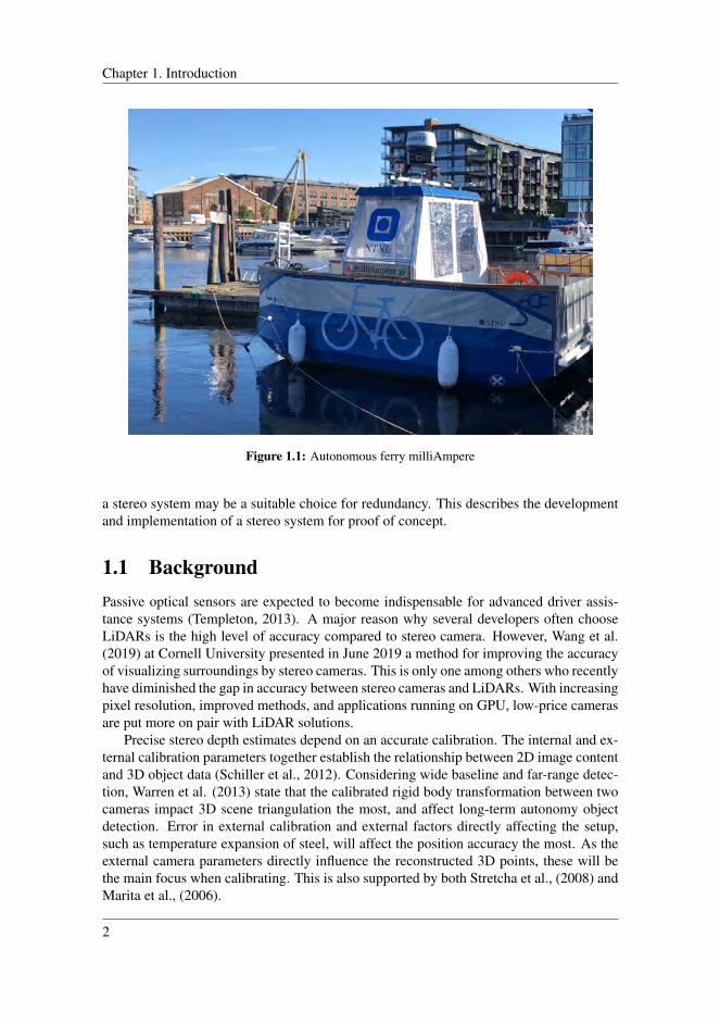
The overall motivation behind this work is to design and construct a stereo system suit-able to integrate on the autonomous ferry milliAmpere. The project is affiliated with theAutoferry project1, which aims to develop new concepts and methods which will enablethe development of autonomous passenger ferries for urban water transport. milliAmpereis equipped with several sensors for situational awareness, where a LiDAR and a radarare utilized for 3D object detection. As the ferry will operate in a confined environment
1https://www.ntnu.edu/autoferry
1
Chapter 1. Introduction
Figure 1.1: Autonomous ferry milliAmpere
a stereo system may be a suitable choice for redundancy. This describes the developmentand implementation of a stereo system for proof of concept.
1.1 BackgroundPassive optical sensors are expected to become indispensable for advanced driver assis-tance systems (Templeton, 2013). A major reason why several developers often chooseLiDARs is the high level of accuracy compared to stereo camera. However, Wang et al.(2019) at Cornell University presented in June 2019 a method for improving the accuracyof visualizing surroundings by stereo cameras. This is only one among others who recentlyhave diminished the gap in accuracy between stereo cameras and LiDARs. With increasingpixel resolution, improved methods, and applications running on GPU, low-price camerasare put more on pair with LiDAR solutions.
Precise stereo depth estimates depend on an accurate calibration. The internal and ex-ternal calibration parameters together establish the relationship between 2D image contentand 3D object data (Schiller et al., 2012). Considering wide baseline and far-range detec-tion, Warren et al. (2013) state that the calibrated rigid body transformation between twocameras impact 3D scene triangulation the most, and affect long-term autonomy objectdetection. Error in external calibration and external factors directly affecting the setup,such as temperature expansion of steel, will affect the position accuracy the most. As theexternal camera parameters directly influence the reconstructed 3D points, these will bethe main focus when calibrating. This is also supported by both Stretcha et al., (2008) andMarita et al., (2006).
2

1.2 Problem description
However, the literature diverge in how to best calibrate the rigid body transformationbetween two cameras. Stretcha et al. (2008) showed that when using a stereo camera, thevariance from the ground truth decrease with decreasing distance to the calibration scene.However, Marita et al. (2006) state that calibration minimizing the projection error onnear distances is unsuited for far range stereo-vision. They further mention that the mostreliable solution is using a calibration scene on distances comparable with the workingrange of the stereo reconstruction application. Regardless of the chosen calibration dis-tance, Abdullah et al., (2019) confirms this hypothesis by stating that independent of thedistance the calibration is performed, the further the objects from the camera, the higherpercentage of errors will be recorded.
Stereo depth estimation require the generation of accurate disparity maps in real-time(Wang et al., 2019). Nevertheless, a disparity map includes noise, and post-processingwith a clustering technique is therefore preferred to extract the resulting world position of3D objects. This can be achieved using both classical clustering techniques or convolu-tional neural networks for object detection and classification. Clustering points into groupsto segment the point cloud is a standard step in processing a captured scene (Nguyen andLe, 2013). Graph-based methods such as hierarchical clustering are robust in dealing withcomplex scenes (Pendleton et al., 2017). Such methods extracts a dynamical number ofclusters and are not dependent on seed points. However, recent advances in computingpower has made deep learning based methods the standard approach for object detection(Li et al., 2019). Deep learning with convolutional neural networks tends to outperformclassical detection methods by recognizing shapes, edges and colors. YOLO is one of thepioneer real-time CNN models, which has demonstrated detection performance improve-ments over R-CNN (Zhao et al., 2019). YOLOv3 outperforms the state of the art detectionalgorithm Faster R-CNN in both sensitivity and computation time (Benjdira et al., 2019).The stereo system will be tested using both YOLOv3 and classical clustering techniques.
1.2 Problem description
The situational awareness of USVs depends on sensors that can perceive the surroundingenvironment. The purpose of this project is to implement an object detection system usinga stereo camera for the autonomous ferry milliAmpere. The project builds on the 5th yearspecialization projects of the two authors (Theimann, 2020)(Ødegard Olsen, 2020) wherea stereo system was set up and tested for shorter distances. While Olsen looked into Stereovision using local methods for autonomous ferry, Theimann complemented by focusing onLiDARs with the project Comparison of depth information from stereo camera and LiDAR.The projects calibrated a stereo setup, and tested the system inside with a controlled staticscene. This thesis incorporate the two projects and continues the research for a far rangestereo system. This thesis addresses the following tasks:
1. Design and implement a stereo system.
2. Perform a LiDAR - stereo camera calibration. Use the LiDAR as ground truth to thedepth measurements.
3
Chapter 1. Introduction
3. Propose a far range calibration procedure and evaluate the obtained parameters.Look at important factors when calibrating at far range.
4. Implement a real-time system for object detection. Make a framework compatiblewith the system running on milliAmpere.
5. Choose a stereo correspondence algorithm suitable for a marine environment. Per-form clustering, isolating the object of interest in the scene.
6. Implement an object recognition procedure using CNN and evaluate the reliabilityof the network.
7. Integrate the system on the autonomous ferry milliAmpere and test it in the oper-ational environment of the vessel. Record relevant data to be used for testing ofdetectors.
8. Analyze the performance of the proposed system.
1.3 Report OutlineThe thesis is divided into two parts. Part I is about stereo vision and the calibration of astereo camera. The part begins with Chapter 2 which describes the theoretical backgroundof stereo vision. The chosen stereo setup is described along with the cameras in use. Chap-ter 3 presents the LiDAR which serves as a ground truth for distance estimates. Chapter 4propose an extrinsic calibration procedure for far range stereo vision. Finally in Chapter5, the resulting parameters are presented, and evaluated based on their performance onscenes of different depths.
Part II is about the application on the ferry in the marine environment. An overviewof the system implemented on milliAmpere is given in Chapter 6. Chapter 7 describesthe techniques used for object detection. The implemented algorithms for depth-mapsand clustering are presented and an evaluation of the reliability is given. In Chapter 8,the results of testing in coastal and harbour environments is presented and discussed. Aconclusion for both parts is given in Chapter 9, along with suggestions for future work.
4

Part I
Stereo vision and calibration
5


Chapter 2Stereo vision
Stereo vision is a computer vision technique used to perceive depth in a scene by combin-ing two or more sensors. With two cameras of known relative position, the 3D positionof points projected on the camera plane can be estimated through triangulation. Workingwith binocular cameras requires an understanding of the calculations and setup, whichboth influence the 3D points probability distribution. As well, the application area andthe choice of algorithms used for computing and solving the correspondence problem willaffect the resulting depth-map and the associated point cloud. The chapter rephrases fromthe two specialization projects written by Theimann (2020) and Olsen (2020).
2.1 Monocular camera
2.1.1 Pinhole model
The pinhole model is one of the most widely used geometric camera models (Hartley andZisserman, 2004). The mathematical model describes the correspondence between real-world 3D points and their projection onto the image plane. Figure 2.1 demonstrates theconcept, where the box represents the camera body. The rear inside of the camera bodyplaces the image plane. The light travels from the top of the scene, straight through theaperture, and projects to the bottom of the camera film. The aperture lets only light raysfrom one direction through at a time. Thus light rays from conflicting directions are filteredout. The camera film, therefore, holds an inverted image of the world.
As there is no lens, the whole image will be in focus. The focus requires an infinitylong exposure time to avoid blur and absence of moving objects. In practice, one equips thecamera with a lens to produce useful images. The pinhole is mathematically convenient,and the geometry of the model is an adequate approximation of the imaging process.
7

Chapter 2. Stereo vision
Figure 2.1: Pinhole model
2.1.2 Camera parameters
The camera parameters describe the relationship between the camera coordinate systemand real-world coordinates. In image transformations, homogeneous coordinates are con-venient for representing geometric transformations. Projective geometry has an extra di-mension to describe Cartesian coordinates in Euclidean space. They allow affine trans-formations and can represent numbers at infinity. Mapping a homogeneous vector to aCartesian space and Cartesian to homogeneous is given by (2.2) and (2.1) respectively(Hartley and Zisserman, 2004).
x =
[uv
]−→ x =
uv1
(2.1)
Figure 2.2: Intrinsic and extrinsic geometry
8

2.1 Monocular camera
x =
uvw
−→ x =
[u/wv/w
](2.2)
The camera parameters are divisible into two groups - internal and external parameters.
Internal parameters
The internal camera parameters comprehend both the intrinsic- and distortion parameters.The intrinsic matrix transforms 3D camera coordinates to 2D homogeneous image coordi-nates. In Figure 2.2, the image plane is parallel to the camera plane at a fixed distance fromthe pinhole. The distance is named the focal length, f . The gray line in the figure repre-sents the principal axis. The principal axis intercepts the image plane in a point called theprincipal point. The perspective projection models the ideal pinhole camera, where eachintrinsic parameter describes a geometric property of the camera
The pinhole model assumes pixels to be square, which may not apply for alternativecamera models. Commonly, cameras are not exact pinhole cameras, and CCD (Charged-coupled device) is the model generally used in digital cameras. Nevertheless, by a fewadjustments, the pinhole model can fit in the CCD model. CCD cameras may have non-square pixels, which can cause an unequal scale factor in each direction. Thus, two addi-tional constants are added, mu and mv . The constants defines the number of pixels perunit distance in image coordinates, u and v direction, respectively.
K =
αu s u00 αv v00 0 1
αu = mufαv = mvfu0 = mupuv0 = mvpv
(2.3)
The adaptive intrinsic matrix is given in (2.3). The parameters αu and αv represents thefocal length in pixel units, and u0 and v0 symbolize the principal point in pixel units (Hart-ley and Zisserman, 2004). The s is named the skew parameter. It is non-zero in cameraswhere the image axes are not perpendicular, usually not the case for today’s cameras.
Image distortion makes straight lines in a scene appear bent in the image. The opticaldistortion is derived in the lens and occurs when lens elements are used to reduce aberra-tions. An ideal pinhole camera does not have a lens, and thus it is not accounted for in theintrinsic matrix. Radial distortion occurs when light rays are bent more near the edges ofthe lens than in the center. Figure 2.3 shows how radial distortion can affect an image. Let(u, v) be the ideal points and (ud, vd), the radial distortion expressed in (2.4).
ud = u+ u[k1(u2 + v2) + k2(u2 + v2)2 + k3(u2 + v2)3...
]vd = v + v
[k1(u2 + v2) + k2(u2 + v2)2 + k3(u2 + v2)3...
] (2.4)
The radial distortion coefficients kn = nth express the type of radial distortion (Zhang,2000).
9

Chapter 2. Stereo vision
(a) Negative radial distortion (b) No distortion (c) Positive radial distortion
Figure 2.3: Radial distortion
Extrinsic parameters
The extrinsic parameters relate the camera plane with the world reference frame, see Fig-ure 2.2. The two coordinate frames are related by the homogeneous transformation matrixT. The matrix consist of a translation matrix and a rotation vector combined.
When describing the intrinsic parameters, the world coordinates were assumed to begiven in the camera frame. To describe the extrinsic parameters, the scene points areexpressed in the world coordinate frame (X,Y, Z). A point, xW in the world frame can beexpressed as a point, xC, in the camera frame by
xC = RxW + t ⇐⇒ xC = TxW
Combining R and t is thus the extrinsic parameters of the camera.The camera matrix is a result of combining the intrinsic parameters K (2.3) with the
extrinsic [R, t]T . It relates world coordinates with pixel coordinates and is notaded withP (2.5).
P =
[Rt
]K (2.5)
2.1.3 Blackfly S GigE
The thesis utilizes two identical cameras in the stereo setup. They are delivered by FLIR,and the camera model is Blackfly S GigE. The selected lens was bought from Edmund
10
2.1 Monocular camera
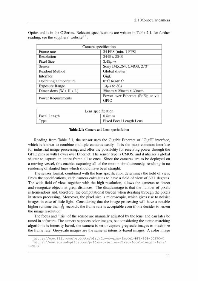
Optics and is in the C Series. Relevant specifications are written in Table 2.1, for furtherreading, see the suppliers’ website1 2.
Camera specificationFrame rate 24 FPS (min. 1 FPS)Resolution 2448 x 2048Pixel Size 3.45µmSensor Sony IMX264, CMOS, 2/3”Readout Method Global shutterInterface GigEOperating Temperature 0◦C to 50◦CExposure Range 13µs to 30sDimensions (W x H x L) 29mm x 29mm x 30mm
Power Requirements Power over Ethernet (PoE); or viaGPIO
Lens specificationFocal Length 8.5mmType Fixed Focal Length Lens
Table 2.1: Camera and Lens spesicifation
Reading from Table 2.1, the sensor uses the Gigabit Ethernet or ”GigE” interface,which is known to combine multiple cameras easily. It is the most common interfacefor industrial image processing, and offer the possibility for receiving power through theGPIO pins or with Power over Ethernet. The sensor type is CMOS, and it utilizes a globalshutter to capture an entire frame all at once. Since the cameras are to be deployed ona moving vessel, this enables capturing all of the motion simultaneously, resulting in norendering of slanted lines which should have been straight.
The sensor format, combined with the lens specification determines the field of view.From the specifications, each camera calculates to have a field of view of 59.1 degrees.The wide field of view, together with the high resolution, allows the cameras to detectand recognize objects at great distances. The disadvantage is that the number of pixelsis tremendous and, therefore, the computational burden when iterating through the pixelsin stereo processing. Moreover, the pixel size is microscopic, which gives rise to noisierimages in case of little light. Considering that the image processing will have a notablehigher runtime than 1
24 seconds, the frame rate is acceptable even if one decides to lessenthe image resolution.
The focus and ”iris” of the sensor are manually adjusted by the lens, and can later betuned in software. The camera supports color images, but considering the stereo matchingalgorithms is intensity-based, the camera is set to capture greyscale images to maximizethe frame rate. Greyscale images are the same as intensity-based images. A color image
1https://www.flir.com/products/blackfly-s-gige/?model=BFS-PGE-50S5C-C2https://www.edmundoptics.com/p/85mm-c-series-fixed-focal-length-lens/
14947/
11

Chapter 2. Stereo vision
transforms into greyscale by summing all the colored layers, R+G+B3 .
The cameras are not waterproof, and together with the high operating temperature, itwill be necessary to make a waterproof and isolating case for protecting the cameras in theoperating environment.
It is preferred to set the manual exposure and focus of the cameras approximately equalto ease the stereo matching. Similar camera parameters will reduce noise when comparingcorresponding pixels in the image processing part. Similar, it is essential to synchronizethe capturing of the two cameras, so images will appear in the correct order when post-processing.
2.2 Stereo setup
Large Baseline
Width of a pixel
Small Baseline
Uncertainty region
Figure 2.5: Illustrating uncertainty depending on the baseline
Representing the 3D world with a discrete camera plane give rise to uncertainty in thedepth estimate. In Figure 2.5 the uncertainty with different baselines is demonstrated. Ingeneral, the uncertainty will decrease with expanding baseline. In addition to the baseline,the vergence angle of the cameras will affect the shape of the uncertainty region. Changingthe angle between the cameras will result in parallel rays give less precise localization of3D points. The accuracy of reconstructed 3D points is thus dependent on both the baselineand the angle, where the width of the probability distribution will decrease with increasingbaseline and vergence angle.
As the accuracy increase with increasing baseline and vergence angle, the search prob-lem becomes more difficult, and the field of view shrinks. The cameras’ angling andbaseline directly influence the field of view (McCabe, 2016). Depth estimation is possibleonly for the overlapping field of view between the two camera views, and in practice, aminimum of 2
3 of each image should overlap. Three different setups are demonstrated inFigure 2.6. Illustrated in green is the field of view. The overlapping field of view willdiminish with a more substantial baseline and concurrently increase the blind spot. Therightmost figure titled Angled demonstrates a solution when using a wide baseline forfar-range detection. When cameras angle inward, the field of view increases and withaldecreases the blind spot.
12

2.2 Stereo setup
Large baseline Small baseline Angled
Figure 2.6: Illustrating field of view in a stereo setup
Another benefit of angling the cameras is that the vergence angle determines a partic-ular fixation point in the scene. When the fixation point is near a target object, it can helpin separating the target objects from distracting surroundings. The working distance, i.e.,how far the setup is from a given object or fixation point, can be calculated depending onthe camera optics.
FOVh = horizontal field of view
h = horizontal sensor size
WD =f ∗ FOVh
h, WD = working distance
f = focal length in metric units of length
The baseline is directly proportional to the horizontal distance from the mounting to theobject. Thus stereo systems with smaller baseline achieve better results when detectingobjects on average distances, whereas broader baseline is preferred with greater distances.As a general rule, the fraction 1
30 is used to estimate the dimension of the baseline (Curtin,2011). For a working distance on 30 meters, the baseline would be about one meter,depending on the cameras’ angling.
Eventually, the setup is a matter of the distance one wants to detect, the width andblind spots, which are all correlated. The factors all define what level of depth-accuracythe system will achieve.
2.2.1 The chosen stereo setupThe stereo setup is designed for the ferry milliAmpere. Considering restrictions and auser-friendly design, the maximum baseline possible is approximately 1.80 meters. Thiscorresponds to a preferred operating distance at 54 meters when cameras are not angled.As presented in Section 2.2 angling the cameras will minimize the error due to the un-certainty region of a pixel. Thus, the cameras were angled, giving a fixation point at 50meters. With a baseline of 1.80 meters, the vergence angle of each camera is calculated byPythagoras to be 1.00 degrees.
Figure 2.7 shows an illustration of the field of view of the stereo camera. This setup
13

Chapter 2. Stereo vision
Figure 2.7: Field of view of stereo setup
Figure 2.8: Stereo setup
14

2.3 Epipolar geometry
gives a blind spot of approximately 1.6 meters in front of the cameras. At 50 meters, ahorizontal FOV of approximately 50 meters is visible.
An attempt of manual measuring the actual baseline was made to get pre-knowledgeabout the resulting calibration parameters. The baseline was measured to be 1800.25 mil-limeters. In addition, the cameras are manually angled 1 degree towards each other. Thusthe expected rotation in Euler angles and translation of the right camera according to theleft would be:
R =[x : 0 y : −2 z : 0
]t =
[−1800 0 0
] (2.6)
As the measurements are done by hand, there are uncertainties in the numbers. However,they give a pointer towards the intended extrinsic calibration parameters
2.3 Epipolar geometry
x1x2
x3
OL OR
xw
Baseline, bx
Left camera view Right camera view
eL
xL xR
eR
Figure 2.9: Epipolar geometry of two cameras
Observing the same world point xW from two relative views gives a strong geometricconstraint on the observed point called the epipolar constraint. By the geometric pinholemodel, triangulation retrieves 3D world coordinates. Figure 2.9 gives an illustration of theepipolar geometry between two cameras. Blue illustrates the image planes, and the pointxW is the world coordinate desired to reconstruct the depth.
The green triangular in Figure 2.9 connects the two optical centers, OL and OR, andthe point xW; it is called the epipolar plane. The baseline, a fixed-length depending on thestereo setup, is the line connecting the two optical centers. The epipolar plane intersectsthrough the two blue image planes forming the red epipolar line in each plane. The epipolarline in the left camera-view intersects the epipole eL and the point xL = (uL, vL).
15

Chapter 2. Stereo vision
The epipolar constraint uses the epipolar line to find pixel correspondences. Capturinga point in one of the cameras, the pixel point in the image generates the epipolar linein the second image. The corresponding pixel must lie on the line. Thus, search forcorrespondences is reduced from a region to a line. The constraint arises by the reasonthat when two cameras capture the same world object, the pixel points, the world point,and the optical centers are all coplanar. The depth is thus directly proportional to thebaseline and the distance between the two pixels capturing the world object.
The epipolar constraint can be represented mathematically by the essential matrix, E,and the fundamental matrix, F. Both the matrices describe the geometric relationshipentirely (Hartley and Zisserman, 2004). The essential matrix depends only on the extrinsicparameters, while the fundamental use image coordinates. In other words, the essentialmatrix represents the constraint in normalized image coordinates, while the fundamentalmatrix represents parameters in pixel coordinates. It is convenient to describe a normalizedimage plane as it represents an idealized camera. Setting z = 1 in front of the projectivecenter, in Figure 2.2, implies a focal length of 1. This lets us describe the imaging processindependently of the camera-specific focal length parameter.
Correspondence between the two homogeneous represented points xL and xR canmathematically be presented in normalized image coordinates (2.7).
xLExR = 0, where E = [tLLR]×RLR (2.7)
The essential matrix is related to the pose between the left and right image planes in Figure2.9. The corresponding rigid body transformation T is defined as
TLR =
[RLR tL
LR0 1
]The fundamental matrix represent the same epipolar constraint in the image plane. It is
the algebraic mapping between a pixel in one image and the epipolar line. Correspondingpixels in the left and right image is again established under the epipolar constraint, thoughvia the intrinsic calibration matrices KL and KR of each camera.
FLR = K−>L ELRK−1R (2.8)
The theory is illustrated in Figure 2.9, where the pixel xL in the left view is mapped to allthe pixels on the epipolar line of the right camera. In practice, every pixel on the epipolarline in the right camera view capturing the world points xW, x1, x2, or x3 can correspondto the one pixel xL in the left view. The problem of selecting the correct matching pixel inthe right view is termed the correspondence problem.
2.4 Correspondence problemIn stereo images, depth is inversely proportional to the disparity between pixels. Theproposition implies that calculating depth is a single trivial equation. However, in order todo the calculation, one must determine for each pixel in one image which pixel in the sec-ond originated from the same 3D world point. This issue is known as the correspondenceproblem and is a central part of binocular vision.
16

2.4 Correspondence problem
Before stereo matching and solving the correspondence problem, the images shouldbe undistorted and rectified to ease the computation of finding corresponding pixels. Theflow chart below illustrates the pipeline for retrieving depth from a stereo camera.
StereoSetup Calibrate
Undistort& rectify
StereoMatching
DisparityMap
Pointcloud
The stereo calibration obtains the rigid body transformation between the two cameras andcan be used to undistort and rectify the images. Rectification is the process of transformingthe two images onto a common image plane, aligning the red epipolar lines in Figure 2.9.It ensures that the corresponding pixels in the image pair are on the same row.
Figure 2.10: Ideal Stereo Geometry
The concept is shown in Figure 2.10. By defining new camera matrices (2.5), the cor-respondence problem is mapped to ideal stereo geometry. The mapping is accomplishedby setting the rotation matrix equal to the identity matrix and expressing the translationalong the x-axis. The ideal stereo geometry is a special case of the epipolar geometrywhere the epipoles are at infinity, meaning x∞L = xR. The cameras will thus have identi-cal orientation, and baseline bx along the x-axis. Ideal stereo geometry gives the followingpixel correspondence;
xL = xR +
f∗bxd00
(2.9)
The pixel correspondence implies that the epipolar lines become horizontal. Looking forcorresponding pixels in the two images boils down to a one-dimensional search.
Various stereo matching algorithms can perform the matching of corresponding pixels.Stereo matching is the task of establishing correspondences between two images of the
17

Chapter 2. Stereo vision
same scene. The pixel distance between matching points is used to create a disparity map.Disparity maps are applicable in various applications with a broad range of input data. Thedepth estimate from the disparity can thus vary remarkably depending upon the propertiesof the data (Praveen, 2019). Therefore, a broad range of algorithms has been developed foracquisition corresponding points and subsequent for matching the points to estimate depth.In general, the methods are classified into local and global approaches. The local methodsconsider pixels in a local neighborhood, while the global methods use the informationpresented in the entire image. Global algorithms are primarily based on the optimizationof a well-behaved-energy function created from the hole image (Liu and Aggarwal, 2005).Because the energy function is defined on all the pixels of the image, global methods areless sensitive to local ambiguities than local methods (Liu and Aggarwal, 2005). In short,the global methods may achieve more accurate disparity maps, while the local methodsyield a less computational cost.
2.4.1 Disparity mapAfter matching corresponding pixels, a disparity map expresses the disparities. Disparitymap, also commonly named range- or depth-map, is a representation of the displacementbetween conjugate pixels in the stereo pair image. It represents the motion between the
Figure 2.11: Example of scene with corresponding grey-scale disparity map and Point cloud
two views. An example of a disparity map is illustrated in Figure 2.11. The smaller thedisparities, the darker the pixels, therefore less motion and longer distance.
X =uL − uR
fZ, Y =
vL − vRf
Z, Z =f ∗ bxd
(2.10)
After extracting the disparity map, the 3D world position of a given object only dependson straightforward mathematics. The triangulation between pixels in the left- (uL, vL) andright-image (uR, vR) is given in (2.10). The position is given in the cameras coordinateframe, where bx is the baseline of the stereo camera, f , the focal length, and d correspondsto the disparity between the two images.
The 3D world coordinates calculated can further be plotted together, creating a pointcloud (Rusu and Cousins, 2011). Point clouds are a means of collating a large number ofsingle spatial measurements into a dataset that can then represent a whole. One can say
18

2.4 Correspondence problem
that the point cloud displays the back-projection of the stereo image pair; an example isdisplayed in Figure 2.11.
2.4.2 Semi-Global MatchingSemi-Global Matching is a method that takes advantage of both local and global properties.The idea is to have a method that is more accurate than local methods and faster thanglobal methods. A Semi-Global Matching approach introduced by Hirchmuller (2005)matches each pixel based on Mutual Information (MI) and the approximation of a globalsmoothness constraint.
The idea is to perform a line optimization by considering pairs of images with knownepipolar geometry. As radiometric differences often occur in stereo image pairs, the dis-similarity of corresponding pixels is modeled using MI. The entropy of the two imagesdefines Mutual Information. It is calculated from the probability distributions of the inten-sities. The model performs a joint histogram of corresponding intensities over the corre-sponding parts based on the epipolar geometry. The resulting definition of MI is definedin (2.11).
MIL,R =∑xL
miL,R((uL, vL), (uR, vR)) (2.11)
miL,R = hL(i) + hR(k)− hL,R(i, k) (2.12)
The probability distributions, hL, hR, and hL,R are summed over the corresponding rowsand columns in the corresponding parts. The last expression hL,R in (2.12) serves as costfor matching the intensities IL(xL) and IR(xR). In stereo images, some pixels may nothave any correspondences, thus the two first expressions in (2.12).
The pixel-wise cost calculation is calculated based on pixel intensity (2.13). The pixel-wise MI matching determines the absolute minimum difference of intensity at xL and xR.
CMI(xL, d) = −miL,R(IL(xL), IR(xR)), xR = xL + d (2.13)
Calculating the cost pixel-wise can often lead to wrong matches, due to, e.g., noise. Forthis reason, a penalization of changes of neighboring disparities is added (2.14). Theimplementation is a smoothness constraint, or energy function.
E(D) =∑xL
C(xL, DxL) +∑
xR∈NxL
P1T (|DxL −DxR | = 1) +∑
xR∈NxL
P2T (|DxL −DxR | > 1)
(2.14)
The equation defines the energy function of the disparity imageD. The first term sums thepixel-wise matching cost. The two following terms add a penalty cost for all pixels in theright image, which are in the neighborhood NxL of the pixel xL in the right image. Theconstant penalty is multiplied for unique matching, i.e., to penalize discontinuities. Theoperator T is defined as the probability distribution of corresponding intensities.
The energy function approximates a global smoothness constraint, and the disparitymap D can be found by minimizing the energy (2.14). However, as this global minimiza-tion (2D) is computational an NP-complete problem for a frequent number of disparity
19

Chapter 2. Stereo vision
maps, the MATLAB implementation uses a slightly modified version. By matching thesmoothed cost in only one dimension, all directions are weighting equally (Hirschmuller,2005). The matching costs are connected by calculating cost paths. Thus the cost of eachpixel is calculated by the sum of all 1D minimum cost paths leading to that pixel. Thematching pixels are the ones that correspond to the minimum cost. The method uses amedian filter with a small window to remove outliers.
Overall, Semi-global matching is calculated for each pixel and is insensitive to illu-mination changes. It is a semi-global method, which is shown to combine global- andlocal-concepts successfully (Hirschmuller, 2011).
20

Chapter 3Ground truth
Ground truth refers to the accuracy of the data collected. In distance estimation, the groundtruth is the real measure and tells how accurate the distance estimation is. When usingstereo vision to acquire depth information, a good ground truth can be obtained from a3D Light Detection and Ranging, LiDAR, sensor. The LiDAR is considered as a highlyaccurate sensor and is adequate as ground truth for long distances. Comparing the pointsobtained by the stereo camera with the ones obtained by the LiDAR gives a reasonableestimate of how exact the stereo depth estimates are.
3.1 Light Detection and Ranging - LiDARLight Detection and Ranging (LiDAR) is a Time of Flight distance sensor. The LiDARemits a laser pulse, and the reflected light energy is returned and recorded by the sensor.The sensor measures the time it takes for the emitted pulse to be reflected to the sensor. Thetravel time is used to calculate the distance to the object that reflects the light. (Velodyne,2019)
Distance =Speed of light · time of flight
2
A 3D LiDAR measures azimuth, elevation and range of the reflection. This gives usa 3D point in spherical coordinates, see illustration in Figure 3.1. In the figure, ϕ is theazimuth angle, θ is the elevation angle and r the distance from the point to the LiDAR.Equation (3.1), expresses a spherical point in Cartesian coordinates in.
X = r cos(θ) sin(ϕ)
Y = r cos(θ) cos(ϕ)
Z = r sin(θ)
(3.1)
The LiDAR outputs a point cloud, and it contains the recorded 3D points given in sphericalcoordinates.
21

Chapter 3. Ground truth
Figure 3.1: Spherical coordinates
Velodyne LiDAR VLP-16
Figure 3.2: Velodyne LiDAR Puck 16
The LiDAR used in this project is the Velodyne LiDAR Puck, VLP 16, see Figure 3.2. Itsspecifications are given in (Velodyne, 2019). It is a compact LiDAR that has a range upto 100 meters, and it has a 360◦ horizontal and 30◦ vertical field of view. It has an rangeaccuracy of ±3 cm making it very accurate. The VLP 16 has 16 laser and detector pairsmounted 2 degrees apart in the vertical direction, starting at -15◦ and ending at 15◦. In thehorizontal direction, the VLP 16 has a resolution between 0.1◦ and 0.4◦, depending on therotation rate. The rotation rate can be chosen as a value between 300 and 1200 RPM.
It is desirable to represent the spherical points given by the sensor in a Cartesian coor-dinate system. This is achieved by creating a coordinate frame centered in the LiDAR, seeFigure 3.3. Here ϕ represents the azimuth angle and θ the elevation angle. As described
22

3.2 LiDAR - stereo camera calibration
(a) Side view (b) Top view
Figure 3.3: The LiDAR coordinate frame
in (3.1) a 3D point p from the LiDAR can be represented in the LiDAR frame as:
p =
rcos(θ)sin(ϕ)rcos(θ)cos(ϕ)
rsin(θ)
where p =[X Y Z
]>(3.2)
3.2 LiDAR - stereo camera calibration
Both the LiDAR and the stereo camera outputs a point cloud relative to the sensor. Toget a ground truth from the LiDAR, a direct comparison of the point clouds is necessary.Thus, the rigid body transformation between the sensors needs to be obtained. To obtaina point cloud from the stereo camera a calibration must be performed. The calibrationis performed by utilizing MATLAB’s stereo calibration app. Wang et al. (2019), amongothers, justifies MATLAB’s stereo calibration method as a high precision calibration methodand uses it as ground truth to their research. Thus, the app is used to calibrate the stereocamera.
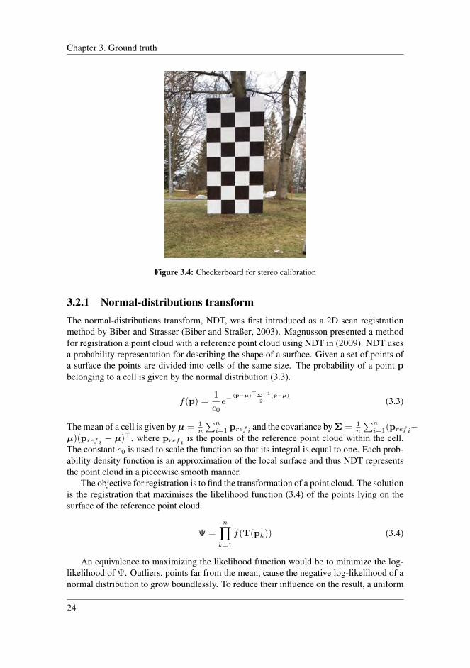
MATLAB’s calibration app requires a checkerboard as a calibration target and statesthat the optimal checkerboard covers approximately twenty percent of the field of view ofthe camera. A checkerboard of the size 1.5×3 meters was constructed to obtain an optimalcalibration. This is the largest size feasible to make, seeing as it needs to be transportable,and the surface needs to be smooth, flat, and rigid. Placing the checkerboard at a depth ofapproximately 7.6 meters, it is visible in both cameras, and a proper stereo calibration canbe performed.
To find the rigid body transformation between the stereo camera and the LiDAR acomparison of the point clouds is made. First, the LiDAR coordinate frame must be trans-formed into the camera frame. Comparing the LiDAR coordinate system in Section 3.3with the camera frame, all the axes must be rotated, and the positive direction of the heightmust be switched. Now, the rigid body transformation is found by a point cloud registra-tion. Point cloud registration is the process of finding the transformation that aligns twopoint clouds of the same scene. The technique used, is the Normal-distribution transform.
23
Chapter 3. Ground truth
Figure 3.4: Checkerboard for stereo calibration
3.2.1 Normal-distributions transformThe normal-distributions transform, NDT, was first introduced as a 2D scan registrationmethod by Biber and Strasser (Biber and Straßer, 2003). Magnusson presented a methodfor registration a point cloud with a reference point cloud using NDT in (2009). NDT usesa probability representation for describing the shape of a surface. Given a set of points ofa surface the points are divided into cells of the same size. The probability of a point pbelonging to a cell is given by the normal distribution (3.3).
f(p) =1
c0e−
(p−µ)>Σ−1(p−µ)2 (3.3)
The mean of a cell is given by µ = 1n
∑ni=1 pref i and the covariance by Σ = 1
n
∑ni=1(pref i−
µ)(pref i − µ)>, where pref i is the points of the reference point cloud within the cell.The constant c0 is used to scale the function so that its integral is equal to one. Each prob-ability density function is an approximation of the local surface and thus NDT representsthe point cloud in a piecewise smooth manner.
The objective for registration is to find the transformation of a point cloud. The solutionis the registration that maximises the likelihood function (3.4) of the points lying on thesurface of the reference point cloud.
Ψ =
n∏k=1
f(T(pk)) (3.4)
An equivalence to maximizing the likelihood function would be to minimize the log-likelihood of Ψ. Outliers, points far from the mean, cause the negative log-likelihood of anormal distribution to grow boundlessly. To reduce their influence on the result, a uniform
24
3.3 The ground truth
distribution is used to represent outliers. The probability of a point p belonging to a cellcan now be rewritten (3.5).
f(p) = c1e− (p−µ)>Σ−1(p−µ)
2 + c2fo (3.5)
The fo is the expected ratio of outliers. By demanding that within a cell, the probabilitymass of f(p) has to be equal to one the constants c1 and c2, can be determined. Thus,given a point cloud and a transformation T(p), a cost function is created (3.6).
C(T(p)) = −n∑k=1
f(T(pk)) (3.6)
Where f(p) is the Gaussian approximation of f(p). When p is transformed by T, the costfunction corresponds to the likelihood of the point lying on the surface of the referencepoint cloud. By solving the equation H∆T(p) = −g, Newton’s method is used to findthe optimal T(p). H is the Hessian and g the gradient of (3.6).
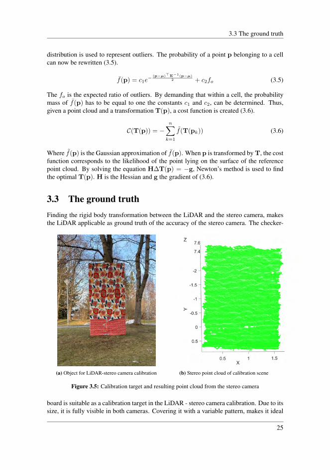
3.3 The ground truthFinding the rigid body transformation between the LiDAR and the stereo camera, makesthe LiDAR applicable as ground truth of the accuracy of the stereo camera. The checker-
(a) Object for LiDAR-stereo camera calibration (b) Stereo point cloud of calibration scene
Figure 3.5: Calibration target and resulting point cloud from the stereo camera
board is suitable as a calibration target in the LiDAR - stereo camera calibration. Due to itssize, it is fully visible in both cameras. Covering it with a variable pattern, makes it ideal
25
Chapter 3. Ground truth
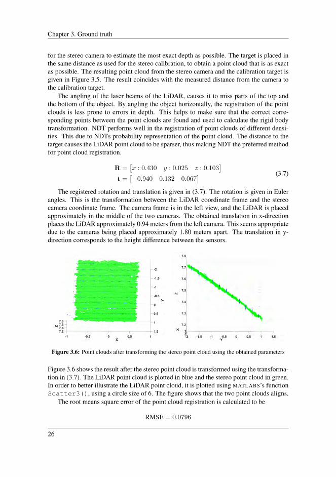
for the stereo camera to estimate the most exact depth as possible. The target is placed inthe same distance as used for the stereo calibration, to obtain a point cloud that is as exactas possible. The resulting point cloud from the stereo camera and the calibration target isgiven in Figure 3.5. The result coincides with the measured distance from the camera tothe calibration target.
The angling of the laser beams of the LiDAR, causes it to miss parts of the top andthe bottom of the object. By angling the object horizontally, the registration of the pointclouds is less prone to errors in depth. This helps to make sure that the correct corre-sponding points between the point clouds are found and used to calculate the rigid bodytransformation. NDT performs well in the registration of point clouds of different densi-ties. This due to NDTs probability representation of the point cloud. The distance to thetarget causes the LiDAR point cloud to be sparser, thus making NDT the preferred methodfor point cloud registration.
R =[x : 0.430 y : 0.025 z : 0.103
]t =
[−0.940 0.132 0.067
] (3.7)
The registered rotation and translation is given in (3.7). The rotation is given in Eulerangles. This is the transformation between the LiDAR coordinate frame and the stereocamera coordinate frame. The camera frame is in the left view, and the LiDAR is placedapproximately in the middle of the two cameras. The obtained translation in x-directionplaces the LiDAR approximately 0.94 meters from the left camera. This seems appropriatedue to the cameras being placed approximately 1.80 meters apart. The translation in y-direction corresponds to the height difference between the sensors.
Figure 3.6: Point clouds after transforming the stereo point cloud using the obtained parameters
Figure 3.6 shows the result after the stereo point cloud is transformed using the transforma-tion in (3.7). The LiDAR point cloud is plotted in blue and the stereo point cloud in green.In order to better illustrate the LiDAR point cloud, it is plotted using MATLABS’s functionScatter3(), using a circle size of 6. The figure shows that the two point clouds aligns.
The root means square error of the point cloud registration is calculated to be
RMSE = 0.0796
26
3.3 The ground truth
This means that the Euclidean distance between the two point clouds after they are alignedis approximately 0.08 meters, i.e. 80 millimeters. A stereo system is expected to havemeter precision at far distances, making the error negligible. The alignment of the pointclouds and the low RMSE show that a valid calibration is made. The LiDAR is used asground truth by utilizing the obtained parameters throughout the following chapters. It isused to evaluate the accuracy of the stereo camera calibrations.
27

Chapter 3. Ground truth
28

Chapter 4Stereo calibration
Calibrating a stereo camera minimizes the measurement uncertainty. It allows for theextraction of precise distance estimations. This chapter presents the theory behind themethod utilized for calibrating a stereo system. The intrinsic and extrinsic parameters areestimated in two separate calibration sessions. Before performing the extrinsic calibrationsfor far range distances, a preliminary work is performed. This is done to give an impressionof the influence of the calibration distance, as discussed in Section 1.1. Based on thefindings, an extrinsic calibration procedure is proposed.
4.1 Monocular camera calibration
Monocular calibration is the process where intrinsic and extrinsic camera parameters areestimated. As well, lens distortion is modeled and corrected. The intrinsic and extrinsicparameters relate the camera coordinate system to the world coordinate frame. Usingthese parameters the size of world objects and the location of the camera in the scenecan be determined. There exist different techniques, but the two main ones, according toZhang (2000) are:
• Photogrammetric calibration: calibration is performed by using an object withknown 3D world points. The correspondences between the real world points andthe corresponding 2D image points can be found by having multiple images of aknown calibration object. The most commonly used object is the checkerboard,where the number of squares and their size is known.
• Self-calibration: no calibration object is used. The camera is moving while thescene remains static. The correspondence between the images is used to estimatethe intrinsic and extrinsic parameters.
29

Chapter 4. Stereo calibration
4.1.1 Zhang’s methodZhang’s method is a calibration technique developed by Zhengyou Zhang at Microsoft Re-search (Zhang, 2000). This method lies between the two main techniques described above,exploiting the advantages of both methods. The only requirement is that the camera hasto observe a planar pattern, typically a checkerboard, in at least two different orientations.The algorithm then detects feature points in the images. Since the plane z = 0 is given bythe pattern itself only 2D metric information is used.
A real-world point and its image point is related by a linear transformation betweenplanes, a homography. For every image, an estimation of the homography can be made.Each image imposes two constraints on the intrinsic and extrinsic parameters. Using morethan three images a unique solution of the parameters can be computed using SingularValue Decomposition. The parameters are refined by minimizing the reprojection errorusing Levenberg-Marquardt Algorithm. An estimation of the radial distortion parametersis calculated by comparing the real pixel values and the ideal ones given by the pinholemodel.
4.1.2 Intrinsic parametersThe internal parameters for each camera were calibrated indoors in a controlled environ-ment. The parameters were estimated using MATLAB’s calibration toolbox. By Zhang’smethod, the app calibrates and provides tools for evaluating and improving the accuracy.The app outputs an estimation of the intrinsic matrices and the distortion coefficients.
Figure 4.1: Image before and after intrinsic calibration
The resulting intrinsic and distortion parameters are given in (4.1) and (4.2), for eachcamera respectively.
KL =
1233.00 0 615.640 1232.45 540.210 0 1
KR =
1233.86 0 636.000 1233.37 536.000 0 1
(4.1)
30

4.2 Preliminary extrinsic stereo calibration
Left cam: k1 = −0.3934, k2 = 0.1816
Right cam: k1 = −0.3910, k2 = 0.1757(4.2)
The two matrices are sufficiently equal and the undistorted images, e.g, Figure 4.1, showsthat the parameters are reasonable. In theory, the intrinsic- and radial distortion parametersfor the two cameras are equal. In practice, this is not feasible due to physical differences,such as manually setting the screw-lenses. The parameters for the focal length are almostidentical, but for the principal point on the x-axis, the values are noticeable divergent.Bear in mind that the principal point is defined to be the image position where the opticalaxis intersects the image plane. Thus, the principal point changes if the camera settingchanges, e.g., changing the focus or zoom. Hence, a small distinction in the rotation of thetwo lenses yields different results for the principal point’s parameters.
Both the skew parameters are set to 0 in MATLAB before calibrating. It is possibleto allow for a non-zero skew, but with newer cameras, the skew-parameters is usuallynegligible. An extra free parameter to calibrate in most cases only give rise to more noisein the calibration. Performing the calibration using a non-zero skew did not give anynoticeable enhancement to the result.
As the thesis focus on far-range depth estimation, the extrinsic stereo parameters arethe most significant and challenging to calibrate (Ødegard Olsen, 2020). The internalparameters will thus remain fixed throughout the rest of the thesis. The internal parametersare easier to re-calibrate in a later stage. The fixed internal parameters makes it easier tocompare the different stereo calibrations.
4.2 Preliminary extrinsic stereo calibrationThe literature diverges regarding extrinsic camera calibration. In preparation of proposinga method, a preliminary stereo calibration is performed to evaluate the research by Maritaet al., (2006), and Stretcha et al. (2008). Stretcha et al. suggests that a higher accuracy isobtained with a decreasing distance to the calibration scene. While Marita et al. found itadvantageous to calibrate at the systems operating distance.
As a starting point, an experiment was set up to evaluate the literature regarding far-range stereo calibration. The stereo setup and test scene from the specialization projectswere used (Theimann, 2020)(Ødegard Olsen, 2020). Calibrating only the external param-eters will give an impression of how the external parameters influences the calibration ondifferent distances. The test scene includes objects placed at a distance of approximately2, 4, and 6 meters. The fixation point of the stereo camera is 4 meters. Thus, the exter-nal parameters are re-calibrated at four distances, 1, 2, 3 and 4 meters respectively. TheLiDAR is used as ground truth for the comparison of the distance estimations.
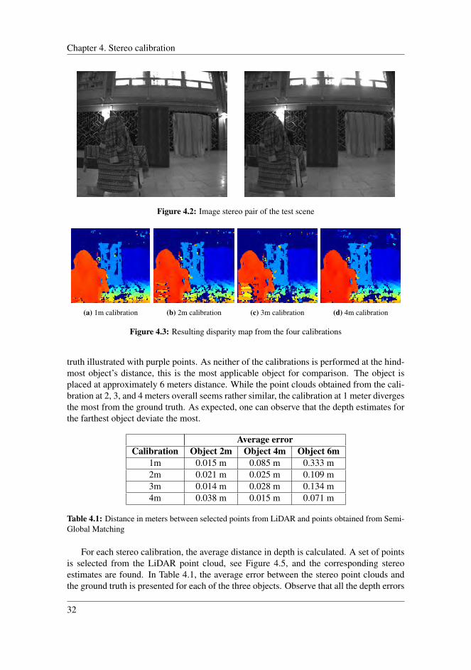
The new external parameters are used to rectify the images before creating a disparitymap of the test scene. The disparity algorithm used, Census Transform, is implemented inOlsen (Ødegard Olsen, 2020), and the resulting disparity maps of the four different cali-brations are illustrated in Figure 4.3. For each disparity map, a point cloud is reconstructedby triangulation, and compared with the point cloud obtained by the LiDAR. Figure 4.4presents the four point-clouds, were each subfigure is a result of the different external pa-rameters. Each stereo point cloud, outlined in green, is presented together with the ground
31
Chapter 4. Stereo calibration
Figure 4.2: Image stereo pair of the test scene
(a) 1m calibration (b) 2m calibration (c) 3m calibration (d) 4m calibration
Figure 4.3: Resulting disparity map from the four calibrations
truth illustrated with purple points. As neither of the calibrations is performed at the hind-most object’s distance, this is the most applicable object for comparison. The object isplaced at approximately 6 meters distance. While the point clouds obtained from the cali-bration at 2, 3, and 4 meters overall seems rather similar, the calibration at 1 meter divergesthe most from the ground truth. As expected, one can observe that the depth estimates forthe farthest object deviate the most.
Average errorCalibration Object 2m Object 4m Object 6m
1m 0.015 m 0.085 m 0.333 m2m 0.021 m 0.025 m 0.109 m3m 0.014 m 0.028 m 0.134 m4m 0.038 m 0.015 m 0.071 m
Table 4.1: Distance in meters between selected points from LiDAR and points obtained from Semi-Global Matching
For each stereo calibration, the average distance in depth is calculated. A set of pointsis selected from the LiDAR point cloud, see Figure 4.5, and the corresponding stereoestimates are found. In Table 4.1, the average error between the stereo point clouds andthe ground truth is presented for each of the three objects. Observe that all the depth errors
32

4.2 Preliminary extrinsic stereo calibration
(a) Stereo calibration at 1m (b) Stereo calibration at 2m
(c) Stereo calibration at 3m (d) Stereo calibration at 4m
Figure 4.4: Resulting point cloud with LiDAR in purple and stereo camera in green
are positive, indicating that the stereo camera overestimates the depth. This applies to allthe objects and the four calibrations.
From the table, the depth errors are relatively small. With the calibration at 1 meter,the object at 6 meters yields an error of 5.6%. At farther distances, an error of 5.6 per-cent is considered reasonable given the projects operating environment on marine water.However, the calibrations at 1, 2, and 4 meters perform the best on the given calibrationdistance. Also, calibration 3 and 4 indicate that shorter distances than the calibration dis-tance are easier to estimate than farther distances.
The depth error for each selected point, on the object placed at 6meters, is displayedin Figure 4.6. The four calibrations are given on the x-axis, and the points present thevariation in the data. Considering both variation and mean, the calibration performed at 4
33

Chapter 4. Stereo calibration
Figure 4.5: Points selected from the LiDAR point cloud.
Figure 4.6: The error of the third object plotted
meters undoubtedly perform better than the other in the given scene.
4.2.1 Discussion
The results present that the closer the calibration scene is to the target object, the betterdepth estimates. Also, more accurate depth estimates are made for targets at shorter dis-tances than the calibrating distances, rather than objects at farther distances. The resultseems to confirm what is stated by Marita et al. (2006). The accuracy of the depth esti-mates is dependent on the distance the calibration is performed at. Thus, it appears that thecalibration should be performed at the operating distance of the stereo system. Consider-ing that the stereo camera overestimated the depth of all the objects, it may be beneficialto overestimate the operating distance while calibrating.
The sections gives an overview of considerations taken into account when calibrating
34
4.3 Extrinsic stereo calibration method
a far range stereo system. It seems that the best result is obtained when performing thecalibration at the operating distance. However, the far-range extrinsic calibration shouldbe conducted at various distances to discard or strengthen the hypothesis further.
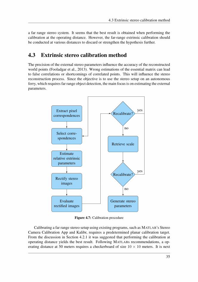
4.3 Extrinsic stereo calibration methodThe precision of the external stereo parameters influence the accuracy of the reconstructedworld points (Fooladgar et al., 2013). Wrong estimations of the essential matrix can leadto false correlations or shortcomings of correlated points. This will influence the stereoreconstruction process. Since the objective is to use the stereo setup on an autonomousferry, which requires far range object detection, the main focus is on estimating the externalparameters.
Extract pixelcorrespondences
Select corre-spondences
Estimaterelative extrinsic
parameters
Rectify stereoimages
Evaluaterectified images
Recalibrate?
Retrieve scale
Recalibrate?
Generate stereoparameters
no
yes
no
yes
Figure 4.7: Calibration procedure
Calibrating a far range stereo setup using existing programs, such as MATLAB’s StereoCamera Calibration App and Kalibr, requires a predetermined planar calibration target.From the discussion in Section 4.2.1 it was suggested that performing the calibration atoperating distance yields the best result. Following MATLABs recommendations, a op-erating distance at 50 meters requires a checkerboard of size 10 × 10 meters. It is next
35
Chapter 4. Stereo calibration
to impossible to create a checkerboard of the preferred size. For this reason, this sectionproposes a method for calibrating a stereo camera using arbitrary scenes. The followingsections presents the theoretical background of the proposed method. A summary of thesteps is given in Figure 4.7.
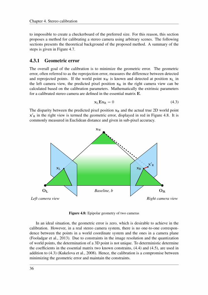
4.3.1 Geometric errorThe overall goal of the calibration is to minimize the geometric error. The geometricerror, often referred to as the reprojection error, measures the difference between detectedand reprojected points. If the world point xW is known and detected at position xL inthe left camera view, the predicted pixel position xR in the right camera view can becalculated based on the calibration parameters. Mathematically the extrinsic parametersfor a calibrated stereo camera are defined in the essential matrix E.
xLExR = 0 (4.3)
The disparity between the predicted pixel position xR and the actual true 2D world pointx′R in the right view is termed the geometric error, displayed in red in Figure 4.8. It iscommonly measured in Euclidean distance and given in sub-pixel accuracy.
OL OR
xW
Baseline, b
Left camera view Right camera view
xLx′R
xR
Figure 4.8: Epipolar geometry of two cameras
In an ideal situation, the geometric error is zero, which is desirable to achieve in thecalibration. However, in a real stereo camera system, there is no one-to-one correspon-dence between the points in a world coordinate system and the ones in a camera plane(Fooladgar et al., 2013). Due to constraints in the image resolution and the quantizationof world points, the determination of a 3D point is not unique. To deterministic determinethe coefficients in the essential matrix two known constrains, (4.4) and (4.5), are used inaddition to (4.3) (Kukelova et al., 2008). Hence, the calibration is a compromise betweenminimizing the geometric error and maintain the constraints.
36
4.3 Extrinsic stereo calibration method
det(E) = 0 (4.4)
2EET − trace(EET )E = 0 (4.5)
4.3.2 Pixel correspondences
Each corresponding pixel pair defines a 3D world point. Pixel correspondences from astereo setup usually are extracted by a featured based method, like the Shi-Tomasi CornerDetector. The Shi-Tomasi Corner Detector (Shi and Tomasi, 1994) is based entirely on theHarris corner detector (G. and Stephens, 1988), with an improvement in the last step.
Shi-Tomasi Corner Detector
Harris Corner Detector or Harris Operator is one of the earliest detectors proposed in 1988by Harris and Stephens (G. and Stephens, 1988). It is an intensity-based mathematicaloperator finding features using corner descriptors in the extraction of features. A corner isthe intersection of two edges, a point where the directions of the two edges change. Hence,a corner can be detected by high variations in the intensity gradient (in both directions). Todetect corners and edges, both the Harris corner detection and Shi-Tomasi Corner Detectoruses a combination of partial derivatives, Gaussian weighting function, and eigenvaluesfrom the matrix representation of the following equation:
erf(∆u,∆v) =∑
(u,v)∈Wm
ω(u, v)[IL(u+ ∆u, v + ∆v)− IR(u, v)]2 (4.6)
The equation (4.6) is indirectly searching for corners. By sweeping a window Wm atposition (u, v) the variation of intensity is calculated for each pixel between the left image,IL(u, v), and the displacement pixel IR(u+∆u, v+∆v). The window function ω(u, v) iseither a rectangular window or Gaussian window, giving weights to pixels underneath. Therectangle window function gives weight 1 to pixels inside the window and 0 otherwise. Inpractice, one can get a noisy response with a binary window function.
The objective is to determine the positions which maximize (4.6). By representing theTaylor expansion as a matrix, subsequently calculating the eigenvalues, weak and robustcorners are detected with a threshold value. Deriving the mathematical expressions step
37
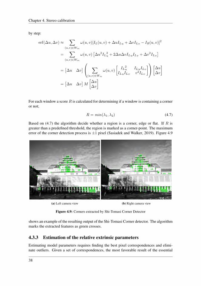
Chapter 4. Stereo calibration
by step:
erf(∆u,∆v) ≈∑
(u,v)∈Wm
ω(u, v)[IL(u, v) + ∆uILu + ∆vILv − IR(u, v)]2
=∑
(u,v)∈Wm
ω(u, v)[∆u2IL
2u + 2∆u∆vILuILv + ∆v2ILv
]
=[∆u ∆v
] ∑(u,v)∈Wm
ω(u, v)
[IL
2u ILuILv
ILuILv v2ILv
][∆u∆v
]
=[∆u ∆v
]M
[∆u∆v
]
For each window a scoreR is calculated for determining if a window is containing a corneror not;
R = min(λ1, λ2) (4.7)
Based on (4.7) the algorithm decide whether a region is a corner, edge or flat. If R isgreater than a predefined threshold, the region is marked as a corner-point. The maximumerror of the corner detection process is ±1 pixel (Sasiadek and Walker, 2019). Figure 4.9
(a) Left camera view (b) Right camera view
Figure 4.9: Corners extracted by Shi-Tomasi Corner Detector
shows an example of the resulting output of the Shi-Tomasi Corner detector. The algorithmmarks the extracted features as green crosses.
4.3.3 Estimation of the relative extrinsic parametersEstimating model parameters requires finding the best pixel correspondences and elimi-nate outliers. Given a set of correspondences, the most favorable result of the essential
38

4.3 Extrinsic stereo calibration method
matrix E minimizes the geometric error. Hence, it minimizes the sum of squares of dis-tances, orthogonal to the variety from each point (Torr and Zisserman, 2000). Estimatingthe essential matrix often gives rise to nonlinear constraints between parameters, makingoptimization a difficult task. Choosing the best correspondences is usually done with esti-mators like Random Sample Consensus (RANSAC) or the modified version M-estimatorSAmple Consensus (MSAC) algorithm. While RANSAC tends to give poor estimateswhen the threshold for inliers is set too high, MSAC is remedied with a new cost func-tion. MSAC was published in 2000 and can robustly estimate the essential matrix frompoint correspondences, providing a 5-10% improvement compared to RANSAC (Torr andZisserman, 2000).
Pixel pairs are chosen based on proximity and similarity; hence mismatches can occur.In theory, all the best matches obey the epipolar geometry, and MSAC aims to removeputative pixel pairs inconsistent with the epipolar geometry, i.e., outliers.
f(D,E) =∏
i=1,...,n
(1√2πσ
)ne−(
∑j=L,R(uj
′i−uji)
2+(vj′i−vji)
2)/(2σ′2) (4.8)
−∑i=1...n
log(f(x(L,R)i
,E, σ))
=∑i=1...n
∑j=L,R
((uj′i − uji)
2 + (vj′i − vji)
2)
(4.9)
e2i =∑j=L,R
(uji − uji)2 + (vji − vji)
2 (4.10)
For N number of times, a randomly chosen set Sm of pixel pairs are chosen to create theessential matrix E. The support for each essential matrix, E, is determined by the inliersin the set Sm.
The images are assumed to include Gaussian distributed noise with zero mean anda uniform standard deviation. The probability density function is given by (4.8), wheren is the number of matches and D the set of matches. For all the corresponding pixelsx(L,R)i
the negative logarithmic likelihood function is (4.9). The true relationship of thestereo camera minimizes the likelihood function (4.9), and thus, the support for each pixelcorrespondence is determined based on finding the maximum likelihood estimation error(4.10). This is termed the MLE error ei, and the estimate x(L,R)i
of the true positionx(L,R)
′i
is minimized for each point i as well as it must satisfy the constraint (4.3).
C =∑i
ρ(e2i ), ρ(e2i ) =
{e2, if e2 < T.
T 2, otherwise.(4.11)
In the end, the support for each essential matrix E is determined by the cost function(4.11). The cost is calculated by summing the MLE error for each inlier in the set Sm, i.e.,correspondences with error an ei below a given threshold T.
The MSAC algorithm for estimating the relative essential matrix can be comprised intothe following steps:
1. Repeat n number of times
39
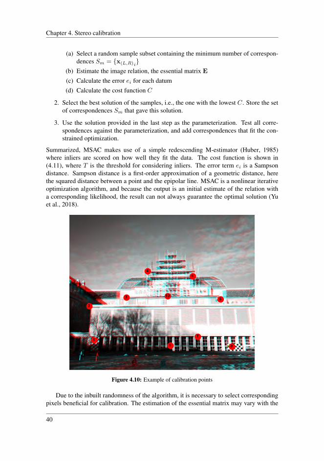
Chapter 4. Stereo calibration
(a) Select a random sample subset containing the minimum number of correspon-dences Sm = {x(L,R)i
}(b) Estimate the image relation, the essential matrix E
(c) Calculate the error ei for each datum(d) Calculate the cost function C
2. Select the best solution of the samples, i.e., the one with the lowest C. Store the setof correspondences Sm that gave this solution.
3. Use the solution provided in the last step as the parameterization. Test all corre-spondences against the parameterization, and add correspondences that fit the con-strained optimization.
Summarized, MSAC makes use of a simple redescending M-estimator (Huber, 1985)where inliers are scored on how well they fit the data. The cost function is shown in(4.11), where T is the threshold for considering inliers. The error term ei is a Sampsondistance. Sampson distance is a first-order approximation of a geometric distance, herethe squared distance between a point and the epipolar line. MSAC is a nonlinear iterativeoptimization algorithm, and because the output is an initial estimate of the relation witha corresponding likelihood, the result can not always guarantee the optimal solution (Yuet al., 2018).
Figure 4.10: Example of calibration points
Due to the inbuilt randomness of the algorithm, it is necessary to select correspondingpixels beneficial for calibration. The estimation of the essential matrix may vary with the
40

4.3 Extrinsic stereo calibration method
same calibration scene and chosen pixel correspondences. The differences may be large.Thus, it is necessary to select the most suitable points of the ones distributed in Figure 4.9.(Yu et al., 2018). Figure 4.10 shows an example of preferred points sent as input to theMSAC algorithm. Some features may be rejected. The algorithm outputs the estimatedrelative essential matrix of the system, which may vary depending on which features arerejected and which are not. Comparing and evaluating the relative essential matrices isbased on the obtained rectified images. Figure 4.11 shows an example of the resulting
Figure 4.11: Example of rectified images
rectification of a scene. The rectification is obtained by running the MSAC algorithm withthe points given in Figure 4.10 as input.
4.3.4 Absolute extrinsic parametersFrom the estimated essential matrix a relative transformation between the two cameras canbe extracted. The parameters are relative, i.e., not given in scale. The angles are absolute,but the translation lacks scale. The absolute extrinsic parameters link the position of thereconstructed 3D points to the real-world coordinate system. To reconstruct the 3D points,matching features in the two images must be found. The images is rectified using therotation between the cameras, and extracted features using Shi-Tomasi Corner Detectorfrom the left image can be tracked into to the right using the Kanade-Lucas-Tomasi featuretracker.
Kanade-Lucas-Tomasi feature tracker
The Kanade-Lucas-Tomasi (KLT) feature tracker is a method for tracking extracted fea-tures presented by Tomasi and Kanade in (1991). Images referring to the same sceneat different viewpoints are strongly related to one another. Thus, it allows for trackinga feature extracted from an image into another image taken at a different angle or time.Consequently, an image sequence obeys the following property
IR(u, v) = IL(u−∆u, v −∆v) (4.12)
41

Chapter 4. Stereo calibration
When two cameras capture a scene from two different viewpoints, moving every point inthe left image makes it possible to obtain the image captured to the right. The displacementd = (∆u,∆v) of a point xR = (u, v), represents the amount of motion between the twoframes. Factors such as occlusion, illumination changes, and the disappearance of pointmake images violate the constraint (4.12). These factors can make the tracking difficult,but at surface markings and non-occluded areas, the property remains invariant.
When tracking a feature from one image to another, a window Wm of pixels is trackedand not a single pixel. Tracking a single pixel is a difficult task due to noise, changes inbrightness, and it can be confused with adjacent pixels. Thus, using windows containingsufficient textures is preferable. By discarding windows where the appearance has changedtoo much, and by modeling the changes as an affine map and not just a single translation,it is possible to make sure that the correct window is tracked. The displacement vector, d,is estimated for small windows. As the images are rectified and taken in the same distanceof the target, any discrepancy not due to translation is considered as an error. The localimage model is given as
IR(xR) = IL(xR − d) + n(xR),
where n is the noise. The displacement vector is chosen to minimize the residue error overa given window Wm. The residue error is given by
erf =
∫Wm
[IL(xR − d)− IR(xR)]2ωdxR,
where, ω is a weighting function.Approximating the intensity function using Taylor series and shortening it to the linear
term yields the following expression.
IL(xR − d) = IL(xR)− g · d
The image gradient is given by g = ( ∂I∂u ,∂I∂v ). Using the new representation of the in-
tensity function the residue function can be rewritten to a quadratic function. Thus, theminimization can be done in closed form. After some rearranging, the following equationis obtained.
d
∫Wm
gg>ωdA =
∫Wm
(IL − IR)gωdA
Gd = e (4.13)
For every corresponding image pairs, the matrix G can be computed by estimating gra-dients and computing their second-order moments of one frame. The two dimensionalvector e can be calculated from the difference between the two images along with the gra-dient. Thus, the displacement d is the solution of (4.13), and feature point can be trackedbetween frames.
Linear triangulation
After extracting corresponding features, their 3D position can be reconstructed using lineartriangulation. Linear triangulation is the process of finding a 3D world point given the
42

4.3 Extrinsic stereo calibration method
pixel coordinates of the point in two different views (Hartley and Zisserman, 2004). Thesolution can be found by utilizing Direct Linear Transformation (DLT). Given a set of2D correspondences, xLi ↔ xRi, the DLT algorithm determines the relation between thecorresponding points.
When using a stereo camera, the corresponding points must satisfy the epipolar con-straint presented in (4.3). The points are captured by two cameras which puts a geometricconstraint on the points given by
xL = PLxW, xR = PRxW
where xL = (uL, vL, wL), P is the camera matrix and xW represents the 3D world coor-dinates. These equations can be combined in order to represent them on the linear formAxW = 0. Using a cross-product, xL × (PLxW) = 0, the homogeneous scale factorcan be eliminated and three equations for each image point can be given. This gives thefollowing
uL(p3>L xW)− (p1>
L ) = 0
vL(p3>L xW)− (p2>
L ) = 0
uL(p2>L xW)− vL(p1>
L ) = 0
where pi>L are the rows in the matrix PL. Thus, an equation on the form AxW = 0 can beconstructed by
A =
uLp3>
L − p1>L
vLp3>L − p2>
LuRp3>
R − p1>R
vRp3>R − p2>
R
(4.14)
Using the Shi-Tomasi Corner Detector and Kanade-Lucas-Tomasi feature tracker, morethan four pixel correspondences are extracted. This results in the equations extracted fromAxW = 0 being over-determined. Due to the discrete camera frame, noise will always bepresent in image coordinates. Hence, there is no exact solution to the system. An approx-imate solution is found by applying a cost function. Minimizing the norm ‖AxW‖ subjectto the constraint ‖xW‖ = 1 the solution is the eigenvector with least eigenvalue of A>A.
From relative to scale
Performing linear triangulation on the corresponding feature points in the two images,allows for a point cloud reconstruction of the scene. Figure 4.12 shows the correspondingfeatures found in a scene captured by the stereo camera. The features are extracted in theleft frame by the Shi-Tomasi Corner Detector, and tracked into the right frame using theKanade-Lucas-Tomasi feature tracker. The resulting point cloud is relative and not givenin scale. To obtain the scale a measurement from the real-world is required.
Using the LiDAR as ground truth, it provides a real-world measurement of the scene.The calibration of the LiDAR-stereo camera in Section 3.2 provides the transformationnecessary to transform the LiDAR into the stereo cameras reference frame. Thus, the Li-DAR measures the actual depth of the scene. NDT presented in Section 3.2.1 calculates
43
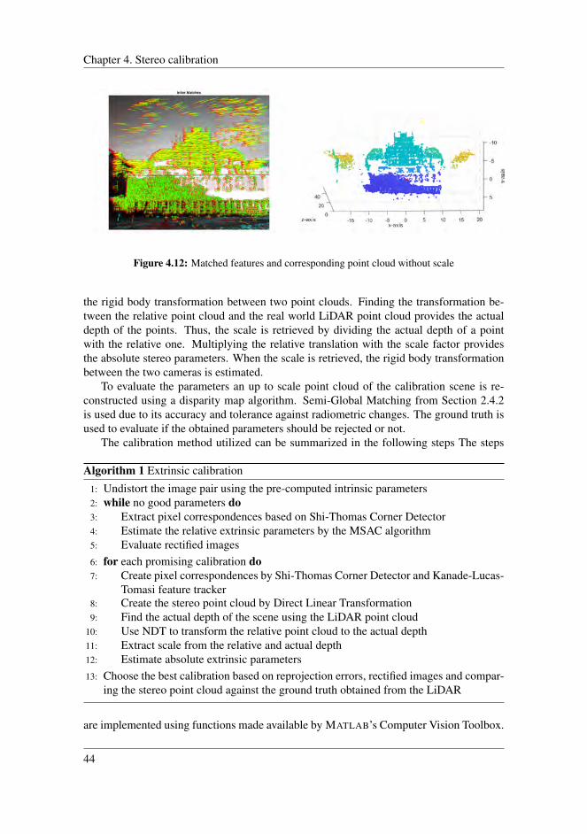
Chapter 4. Stereo calibration
Figure 4.12: Matched features and corresponding point cloud without scale
the rigid body transformation between two point clouds. Finding the transformation be-tween the relative point cloud and the real world LiDAR point cloud provides the actualdepth of the points. Thus, the scale is retrieved by dividing the actual depth of a pointwith the relative one. Multiplying the relative translation with the scale factor providesthe absolute stereo parameters. When the scale is retrieved, the rigid body transformationbetween the two cameras is estimated.
To evaluate the parameters an up to scale point cloud of the calibration scene is re-constructed using a disparity map algorithm. Semi-Global Matching from Section 2.4.2is used due to its accuracy and tolerance against radiometric changes. The ground truth isused to evaluate if the obtained parameters should be rejected or not.
The calibration method utilized can be summarized in the following steps The steps
Algorithm 1 Extrinsic calibration
1: Undistort the image pair using the pre-computed intrinsic parameters2: while no good parameters do3: Extract pixel correspondences based on Shi-Thomas Corner Detector4: Estimate the relative extrinsic parameters by the MSAC algorithm5: Evaluate rectified images6: for each promising calibration do7: Create pixel correspondences by Shi-Thomas Corner Detector and Kanade-Lucas-
Tomasi feature tracker8: Create the stereo point cloud by Direct Linear Transformation9: Find the actual depth of the scene using the LiDAR point cloud
10: Use NDT to transform the relative point cloud to the actual depth11: Extract scale from the relative and actual depth12: Estimate absolute extrinsic parameters13: Choose the best calibration based on reprojection errors, rectified images and compar-
ing the stereo point cloud against the ground truth obtained from the LiDAR
are implemented using functions made available by MATLAB’s Computer Vision Toolbox.
44

Chapter 5Calibration results
The far range calibration method described in Chapter 4 is tested on different distances.Considering the operating distance of the stereo camera, it appears that the calibrationshould be performed at 50 meters. However, to test if the accuracy of the depth estimatesis dependent on the distance the calibration is performed at, the calibrations are performedat 10, 20, 30, 40, 50, 60, and 70 meters. To evaluate the resulting parameters, they aretested on scenes of various depths. The LiDAR serves as a ground truth.
5.1 Resulting parameters
(a) Scene 10m (b) Scene 20m (c) Scene 30m (d) Scene 40m
(e) Scene 50m (f) Scene 60m (g) Scene 70m
Figure 5.1: Calibration scene
45
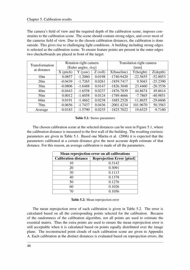
Chapter 5. Calibration results
The camera’s field of view and the required depth of the calibration scene, imposes con-straints to the calibration scene. The scene should contain strong edges, and cover most ofthe cameras field of view. Due to the chosen calibration distances, the calibration is doneoutside. This gives rise to challenging light conditions. A building including strong edgesis selected as the calibration scene. To ensure feature points are present in the outer edgestwo checkerboards are placed in front of the target.
Transformationat distance
Rotation right camera[Euler angles, deg]
Translation right camera[mm]
X (pitch) Y (yaw) Z (roll) X(baseline) Y(height) Z(depth)10m 0.0857 -1.2060 0.0198 -1740.9420 -22.5655 -52.005320m -0.0439 -1.7265 0.0261 -1859.7417 9.5043 -25.239030m -0.0806 -1.6488 0.0147 -1826.3048 23.4460 -20.353640m -0.0443 -1.6558 0.0237 -1876.7839 44.8674 49.861450m 0.0012 -1.6058 0.0124 -1789.4666 -7.7865 -40.985160m 0.0191 -1.4662 0.0238 -1685.2528 -11.8655 -29.660670m -0.0656 -1.7437 0.0436 -2001.4234 101.9670 50.3563
Average -0.0183 -1.5790 0.0235 -1825.7022 19.6525 -9.7180
Table 5.1: Stereo parameters
The chosen calibration scene at the selected distances can be seen in Figure 5.1, wherethe calibration distance is measured to the first wall of the building. The resulting extrinsicparameters are given in Table 5.1. Based one Marita et al. (2006) it is expected that theparameters calibrated at a certain distance give the most accurate depth estimate of thatdistance. For this reason, an average calibration is made of all the parameters.
Mean reprojection error on all calibrationsCalibration distance Reprojection Error [pixel]
10 0.314220 0.309130 0.111340 0.137850 0.127660 0.102670 0.1056
Table 5.2: Mean reprojection error
The mean reprojection error of each calibration is given in Table 5.2. The error iscalculated based on all the corresponding points selected for the calibration. Becauseof the randomness of the calibration algorithm, not all points are used to estimate theessential matrix. Thus the extra points are used to ensure the mean reprojection error isstill acceptable when it is calculated based on points equally distributed over the imageplane. The reconstructed point clouds of each calibration scene are given in AppendixA. Each calibration at the distinct distances is evaluated based on reprojection errors, the
46

5.1 Resulting parameters
rectified images, and the constructed point cloud of the calibration scene compared to theLiDAR
5.1.1 EvaluationAt 10 meters, the calibration scene is challenging, see Figure 5.1a. There are not enoughstrong corners to get useful feature points evenly distributed in the scene. Extracting pixelcorrespondences is only possible around the checkerboard, which is too small of a regionof the image frame. Thus, the parameters are expected to deviate some from the others.The same goes for the calibration at 60 and 70 meters. The two scenes contain too muchof the sky and the ground, which both are impractical for extracting satisfactory cornerpoints.
Based on the stereo setup described in Section 2.2.1 the parameters are expected to bein the range of
R =[x : 0 y : −2 z : 0
]t =
[−1800 0 0
]Most of the calibrations are within the range of the expected result, with the 10, 40, and 70meters calibration showing the most divergence. Considering (2.10) in Section 2.4.1 thebaseline i.e., the translation in x-direction directly influences the estimated depth. Withthis in mind, the 40, 60, and 70 meters calibrations are expected to have a lower depthaccuracy than the other parameters.
To inspect the extrinsic parameters, all the calibration parameters are plotted togetherin Figure 5.2. For each disparity on the x-axis, the corresponding depth is calculated.Figure 5.2a shows the entire graph, where 5.2b and 5.2c is zoomed in on the smallest andgreatest disparities, respectively. The parameters estimates different depths of the samedisparity. The biggest divergence is in the smallest disparities. The disparity is calculatedbased on the rectified images of a scene, which is dependent on the extrinsic parameters.In a real-world scenario, the same 3D-object corresponds to different disparities dependingon the calibration parameters. I.e., the calibrations may give the same depth result even ifthe disparity is different, see the formula for depth (2.10) in Section 2.4.1.
The corresponding pixels used to estimate the essential matrix are extracted using theShi-Tomasi Corner Detector, which has a maximum error of±1 pixel. In the plot, the gra-dient decreases with increasing disparity. Hence, at farther distances an error of one pixelcorresponds to a higher inaccuracy. When calibrating at farther distances, an error of onepixel is far more critical than for shorter distances. Thus, making calibration on far rangetargets more sensitive to errors. The graph stabilizes at around 10 pixels, correspondingto 250 meters. To minimize inaccuracies of the depth, it is reasonable to set the minimumdisparity around 10 pixels. Given by the plot, the minimum distance is 2 meters. This isdue to the wide baseline giving rise to a blind spot in front of the cameras.
The mean reprojection errors in Table 5.2 are all reasonable low. The reprojection errorand the value of the parameters alone do not say much of the quality of the calibrations.Of course, the reprojection error needs to be reasonably low, and the parameters within agiven range, but it does not directly express how exact the depth estimates are. From avisual inspection of the point clouds in Appendix A, they all seem to estimate the depthof the calibration scene quite satisfyingly. The stereo parameters at 40 and 20 meters
47
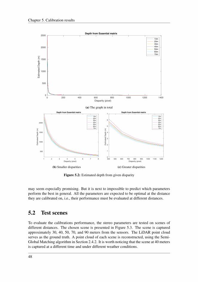
Chapter 5. Calibration results
0 200 400 600 800 1000 1200 1400
Disparity (pixel)
0
500
1000
1500
2000
2500
Estim
ate
d D
ep
th (
m)
Depth from Essential matrix
10m
20m
30m
40m
50m
60m
70m
(a) The graph in total
1 2 3 4 5 6 7 8
Disparity (pixel)
500
1000
1500
2000
Estim
ate
d D
epth
(m
)
Depth from Essential matrix
10m
20m
30m
40m
50m
60m
70m
(b) Smaller disparities
400 500 600 700 800 900 1000 1100 1200
Disparity (pixel)
0
1
2
3
4
5
6
7
Estim
ate
d D
epth
(m
)
Depth from Essential matrix
10m
20m
30m
40m
50m
60m
70m
(c) Greater disparities
Figure 5.2: Estimated depth from given disparity
may seem especially promising. But it is next to impossible to predict which parametersperform the best in general. All the parameters are expected to be optimal at the distancethey are calibrated on, i.e., their performance must be evaluated at different distances.
5.2 Test scenes
To evaluate the calibrations performance, the stereo parameters are tested on scenes ofdifferent distances. The chosen scene is presented in Figure 5.3. The scene is capturedapproximately 30, 40, 50, 70, and 90 meters from the sensors. The LiDAR point cloudserves as the ground truth. A point cloud of each scene is reconstructed, using the Semi-Global Matching algorithm in Section 2.4.2. It is worth noticing that the scene at 40 metersis captured at a different time and under different weather conditions.
48

5.2 Test scenes
Figure 5.3: Test scene
In addition to a visual inspection, the translation in z-direction between the point cloudand ground truth is registered. To measure the error, the stereo point cloud is mapped ontothe LiDAR point cloud. The transformation is registered by NDT. Noise is cut out of thepoint clouds to calculating the error transformation. The translations in the z-direction areused to evaluate the calibration accuracy in depth.
5.2.1 Results
The stereo and LiDAR point clouds of the scenes are plotted together and given in Ap-pendix B. The error in depth of each calibration on the different test scenes is given in
Average depth errorCalibration Scene 30m Scene 40m Scene 50m Scene 70m Scene 90m
7.6 m 3.54 m 2.46 m 8.75 m 15.79 m 26.49 m10 m 5.56 m 4.60 m 16.91 m 35.56 m 65.86 m20 m 1.23 m 0.94 m 1.65 m 1.32 m 1.25 m30 m 1.43 m 0.50 m 2.86 m 4.09 m 6.59 m40 m 2.40 m 0.60 m 4.13 m 5.51 m 8.30 m50 m 1.22 m 0.71 m 3.11 m 5.15 m 8.71 m60 m 0.94 m 0.78 m 4.28 m 9.21 m 17.81 m70 m 3.45 m 1.97 m 5.21 m 5.56 m 6.87 mAvg 2.27 m 0.65 m 5.37 m 8.36 m 12.64 m
Table 5.3: Distance in meters between stereo point cloud and ground truth
Table 5.3. The calibration obtained using MATLAB’s stereo camera calibration app is in-cluded to illustrate the far range accuracy of a pre-existing calibration method. It shouldbe noted that all the parameters overestimate the distance to the target. Figure 5.4 showsthe resulting plot of the error in the depth of each calibration. Two apparent outliers are
49
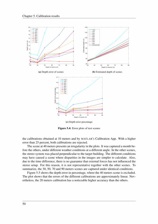
Chapter 5. Calibration results
30 40 50 60 70 80 90
Depth of scene (m)
0
2
4
6
8
10
12
14
16
18
20D
ep
th e
rro
r (m
)
7.6m
10m
20m
30m
40m
50m
60m
70m
Avg
(a) Depth error of scenes
30 40 50 60 70 80 90
Depth of scene (m)
20
40
60
80
100
120
140
160
Estim
ate
d d
epth
(m
)
7.6m
10m
20m
30m
40m
50m
60m
70m
Avg
Ground truth
(b) Estimated depth of scenes
30 40 50 60 70 80 90
Depth of scene (m)
0
0.1
0.2
0.3
0.4
0.5
0.6
0.7
De
pth
err
or
pe
rce
nta
ge
7.6m
10m
20m
30m
40m
50m
60m
70m
Avg
(c) Depth error percentage
Figure 5.4: Error plots of test scenes
the calibrations obtained at 10 meters and by MATLAB’s Calibration App. With a highererror than 25 percent, both calibrations are rejected.
The scene at 40 meters presents an irregularity in the plots. It was captured a month be-fore the others, under different weather conditions at a different angle. In the other scenes,the stereo system was placed perpendicular to the target building. The different conditionsmay have caused a scene where disparities in the images are simpler to calculate. Also,due to the time difference, there is no guarantee that external forces has not influenced thestereo setup. For this reason, it is not representative together with the other scenes. Tosummarize, the 30, 50, 70 and 90 meters scenes are captured under identical conditions.
Figure 5.5 shows the depth error in percentage, where the 40 meters scene is excluded.The plot shows that the errors of the different calibrations are approximately linear. Nev-ertheless, the 20 meters calibration has a noticeable higher accuracy than the others.
50
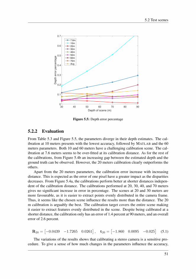
5.2 Test scenes
30 40 50 60 70 80 90
Depth of scene (m)
0
0.1
0.2
0.3
0.4
0.5
0.6
0.7
De
pth
err
or
pe
rce
nta
ge
7.6m
10m
20m
30m
40m
50m
60m
70m
Avg
Figure 5.5: Depth error percentage
5.2.2 EvaluationFrom Table 5.3 and Figure 5.5, the parameters diverge in their depth estimates. The cal-ibration at 10 meters presents with the lowest accuracy, followed by MATLAB and the 60meters parameters. Both 10 and 60 meters have a challenging calibration scene. The cal-ibration at 7.6 meters seems to be over-fitted at its calibration distance. As for the rest ofthe calibrations, from Figure 5.4b an increasing gap between the estimated depth and theground truth can be observed. However, the 20 meters calibration clearly outperforms theothers.
Apart from the 20 meters parameters, the calibration error increase with increasingdistance. This is expected as the error of one pixel have a greater impact as the disparitiesdecreases. From Figure 5.4a, the calibrations perform better at shorter distances indepen-dent of the calibration distance. The calibrations performed at 20, 30, 40, and 70 metersgives no significant increase in error in percentage. The scenes at 20 and 30 meters aremore favourable, as it is easier to extract points evenly distributed in the camera frame.Thus, it seems like the chosen scene influence the results more than the distance. The 20m calibration is arguably the best. The calibration target covers the entire scene makingit easier to extract features evenly distributed in the scene. Despite being calibrated at ashorter distance, the calibration only has an error of 1.4 percent at 90 meters, and an overallerror of 2.6 percent.
R20 =[−0.0439 −1.7265 0.0261
], t20 =
[−1.860 0.0095 −0.025
](5.1)
The variations of the results shows that calibrating a stereo camera is a sensitive pro-cedure. To give a sense of how much changes in the parameters influence the accuracy,
51
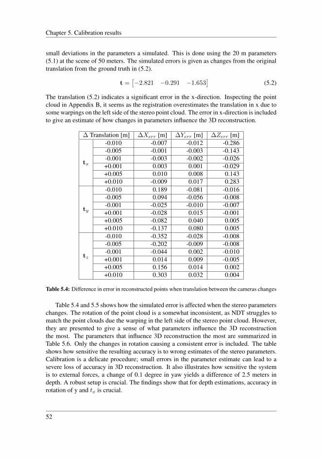
Chapter 5. Calibration results
small deviations in the parameters a simulated. This is done using the 20 m parameters(5.1) at the scene of 50 meters. The simulated errors is given as changes from the originaltranslation from the ground truth in (5.2).
t =[−2.821 −0.291 −1.653
](5.2)
The translation (5.2) indicates a significant error in the x-direction. Inspecting the pointcloud in Appendix B, it seems as the registration overestimates the translation in x due tosome warpings on the left side of the stereo point cloud. The error in x-direction is includedto give an estimate of how changes in parameters influence the 3D reconstruction.
∆ Translation [m] ∆Xerr [m] ∆Yerr [m] ∆Zerr [m]
tx
-0.010 -0.007 -0.012 -0.286-0.005 -0.001 -0.003 -0.143-0.001 -0.003 -0.002 -0.026+0.001 0.003 0.001 -0.029+0.005 0.010 0.008 0.143+0.010 -0.009 0.017 0.283
ty
-0.010 0.189 -0.081 -0.016-0.005 0.094 -0.056 -0.008-0.001 -0.025 -0.010 -0.007+0.001 -0.028 0.015 -0.001+0.005 -0.082 0.040 0.005+0.010 -0.137 0.080 0.005
tz
-0.010 -0.352 -0.028 -0.008-0.005 -0.202 -0.009 -0.008-0.001 -0.044 0.002 -0.010+0.001 0.014 0.009 -0.005+0.005 0.156 0.014 0.002+0.010 0.303 0.032 0.004
Table 5.4: Difference in error in reconstructed points when translation between the cameras changes
Table 5.4 and 5.5 shows how the simulated error is affected when the stereo parameterschanges. The rotation of the point cloud is a somewhat inconsistent, as NDT struggles tomatch the point clouds due the warping in the left side of the stereo point cloud. However,they are presented to give a sense of what parameters influence the 3D reconstructionthe most. The parameters that influence 3D reconstruction the most are summarized inTable 5.6. Only the changes in rotation causing a consistent error is included. The tableshows how sensitive the resulting accuracy is to wrong estimates of the stereo parameters.Calibration is a delicate procedure; small errors in the parameter estimate can lead to asevere loss of accuracy in 3D reconstruction. It also illustrates how sensitive the systemis to external forces, a change of 0.1 degree in yaw yields a difference of 2.5 meters indepth. A robust setup is crucial. The findings show that for depth estimations, accuracy inrotation of y and tx is crucial.
52

5.3 Discussion
∆ Rotation [deg] ∆Xerr[m] ∆Yerr [m] ∆Zerr [m]
X (Pitch)
+0.3 0.285 -1.170 0.113+0.2 0.455 -0.734 0.038+0.1 -0.067 -0.185 -0.009-0.1 0.066 -0.384 -0.087-0.2 -0.452 -1.090 -0.039-0.3 -0.629 -1,173 -0.045
Y (Yaw)
+0.3 -1.241 -0.595 -9.730+0.2 0.068 -0.194 -6.188+0.1 -3.235 -1.931 -2.422-0.1 -0.000 0.136 2.611-0.2 -0.005 0.156 5.000-0.3 -0.141 0.152 7.185
Z (Roll)
+0.3 3.224 0.535 -0.088+0.2 3.228 0.606 -0.132+0.1 1.855 0.359 -0.059-0.1 -1.093 -0.222 -0.020-0.2 -2.495 -0.242 -0.095-0.3 -3.242 -0.102 -0.181
Table 5.5: Difference in error in reconstructed points when orientation between the cameras changes
ExtrinsicParameter Error
Error of the reconstructed 3D coordinateX (lateral offset) Y (height) Z (depth)
tx small error small error criticalty error small error ≈ 0tz error small error ≈ 0
X (Pitch) - - ≈ 0Y (Yaw) - - criticalZ (Roll) critical small error ≈ 0
Table 5.6: Extrinsic parameters errors’ effect on 3D reconstruction
5.3 Discussion
Calibration is a sensitive procedure. Overall, the depth errors were higher than expected.Most parameters has an error that stabilizes around 10 percent when the distance is in-creasing. However, there are some significant outliers. The accuracy of 3D reconstructionwas shown to be sensitive to wrong estimations of rotation of y and tx.
The calibration procedure is based on a set of assumptions and approximations. Firstthe Shi-Tomasi corner detector has a maximum error of ±1 pixels. An error of one pixelhas a high impact of the accuracy as the distance increases. The extraction of feature pointsat distances as high as 70 meters makes it challenging to accurately estimate the parame-ters. In addition, the feature points used are manually extracted. Thus, the result is relianton how careful the user is in selecting the points. A very careful selection of the used
53

Chapter 5. Calibration results
calibration images and a different placing of the calibration board may also contribute tokeep this error smaller. For the extraction of scale, no normalization was performed on theparameters used in the linear triangulation procedure. Due to the numerical estimation inDLT, the entries of A (4.14) should preserve to have similar magnitude. Thus, in retrospectthe results of the triangulation may benefit from a normalization of the camera matrix. Asthe intrinsic parameters obtained from the MATLAB calibration are given in millimeters,they are of a higher magnitude than the other parameters; the homogeneous coordinate wand the relative extrinsic estimated matrix given in the range of 0-1.
The calibration at 50 and 60 meters was expected to give the best result for the testscene at the operating distance of the stereo camera, i.e. 50 meters. However, the highestaccuracy on the operating distance was obtained from the 20 and 30 meters calibration.Overall, of all the different parameters the ones obtained at 20 and 30 meters gave thehighest accuracy. The 20 meters calibration resulted in an average error of only 2.6 percent.Which is noticeable better compared to Wang et al., (2019), which achieved an accuracy of74% at 30 meters putting their approach on par with LiDAR. The calibration scenes at 20and 30 meters has the most favorable distribution of feature points for calibration. Thus,the results indicates that using an appropriate calibration scene is of higher importancethan the depth of the scene. A scene covering the entire FOV, makes it possible to extractcorresponding pixels distributed in the whole frame.
The errors are expected to be higher if testing in the operational environment. In amarine environment, there is less strong corners to match and reflection from the watermakes the stereo matching burdensome. Another reason is that the test scenes used, maybe too similar to the calibration scene. All the parameters should therefore have been testedin a marine environment to see the actual performance in the operational environment.Due to COVID-19 it was not possible to access the equipment necessary to acquire a moresuitable test scene.
From the change of accuracy between the 40 meter test scene and the others scenes,there may have been some external factors influencing the stereo setup. The 40 meterscene was captured in early February, and the other test scenes were captured in late April.In the time between, the physical stereo system has been subjected to wear and tear dueto transportation. The camera had to be moved around more than preferable. This mayhave caused changes to the configurations, including the angling of the cameras and themanually set exposure and zoom. Changes like this will directly influence the uncertaintyof the depth estimates.
54
Part II
Application in marineenvironment
55


Chapter 6System overview
The intended use of the stereo camera is visual vessel detection for the autonomous ferrymilliAmpere. This chapter introduces a stereo system for object detection in a marineenvironment. Two clustering techniques are implemented; hierarchical clustering usingEuclidean distance and a convolution neural network (CNN). The network is used forclassification, and its bounding boxes is combined with the disparity map to extract 3Dpositions of objects. The Euclidean clustering processes the raw point cloud reconstructedfrom the disparity map. This chapter gives an overview of the complete system while thefollowing chapter goes into detail of the implementation of the techniques. Furthermore,the stereo system is combined with the system running on milliAmpere to output the de-tected objects in a common world frame. The system is implemented for testing the stereocameras performance in milliAmperes operating environment.
Figure 6.1: Example of scene captured by the stereo camera
57
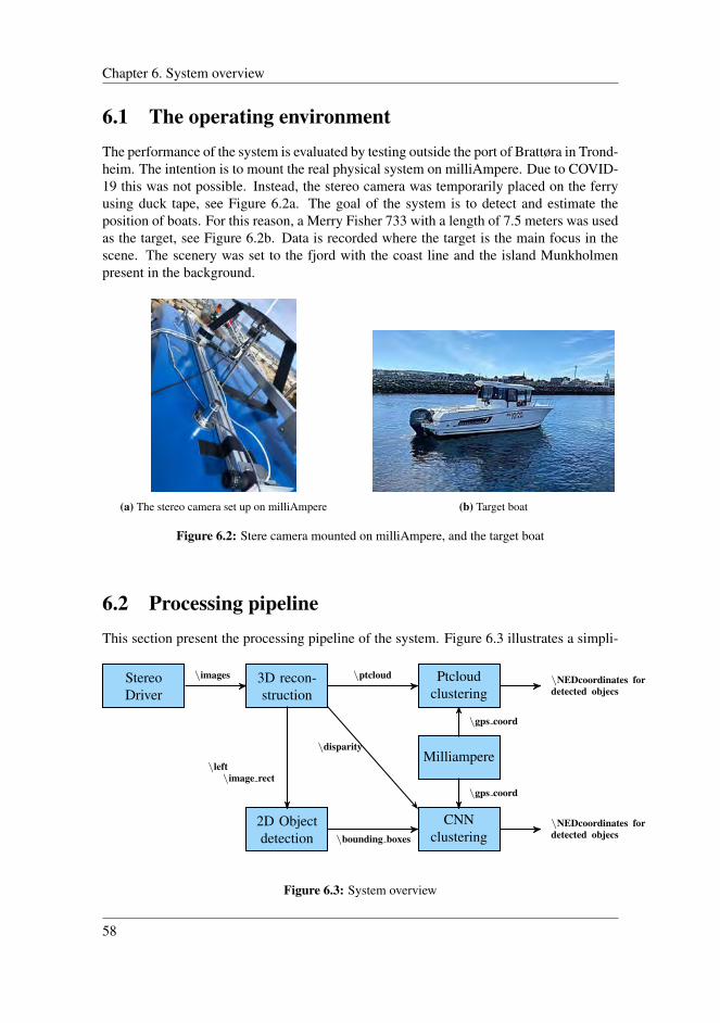
Chapter 6. System overview
6.1 The operating environmentThe performance of the system is evaluated by testing outside the port of Brattøra in Trond-heim. The intention is to mount the real physical system on milliAmpere. Due to COVID-19 this was not possible. Instead, the stereo camera was temporarily placed on the ferryusing duck tape, see Figure 6.2a. The goal of the system is to detect and estimate theposition of boats. For this reason, a Merry Fisher 733 with a length of 7.5 meters was usedas the target, see Figure 6.2b. Data is recorded where the target is the main focus in thescene. The scenery was set to the fjord with the coast line and the island Munkholmenpresent in the background.
(a) The stereo camera set up on milliAmpere (b) Target boat
Figure 6.2: Stere camera mounted on milliAmpere, and the target boat
6.2 Processing pipelineThis section present the processing pipeline of the system. Figure 6.3 illustrates a simpli-
StereoDriver
3D recon-struction
2D Objectdetection
Ptcloudclustering
CNNclustering
Milliampere\left\image rect
\images \ptcloud \NEDcoordinates fordetected objecs
\bounding boxes\NEDcoordinates fordetected objecs
\disparity
\gps coord
\gps coord
Figure 6.3: System overview
58
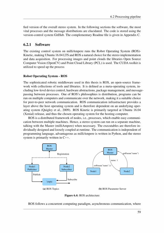
6.2 Processing pipeline
fied version of the overall stereo system. In the following sections the software, the mostvital processes and the message distributions are elucidated. The code is stored using theversion-control system GitHub. The complementary Readme file is given in Appendix C.
6.2.1 SoftwareThe existing control system on milliAmpere runs the Robot Operating System (ROS)-Kinetic, making Ubuntu 16.04 LTS and ROS a natural choice for the stereo implementationand data acquisition. For processing images and point clouds the libraries Open SourceComputer Vision (OpenCV) and Point Cloud Library (PCL) is used. The CUDA toolkit isutilized to speed up the process
Robot Operating System - ROS
The sophisticated robotic middleware used in this thesis is ROS, an open-source frame-work with collections of tools and libraries. It is defined as a meta-operating system, in-cluding low-level device control, hardware abstractions, package management, and message-passing between processes. One of ROS’s philosophies is distribution, programs can berun on multiple computers and communicate over the network, making it a suitable choicefor peer-to-peer network communication. ROS communication infrastructure provides alayer above the host operating system and is therefore dependent on an underlying oper-ating system (Quigley et al., 2009). ROS Kinetic is primarily targeted at Ubuntu 16.04(Xenial) release, and thus the chosen operating system for the hosting computer.
ROS is a distributed framework of nodes, i.e., processes, which enable easy communi-cation between multiple machines. Hence, a stereo system can run on a separate machine,talking with the Master (milliAmpere) when necessary. The executables are therefore in-dividually designed and loosely coupled at runtime. The communication is independent ofprogramming language, advantageous as milliAmpere is written in Python, and the stereosystem is primarily written in C++.
ROSMaster
Node1Publisher
Node2Subscriber
\topic
Registration
Publish
Subscribe
(a) ROS Topics
ROSMaster
Node1 Node2
setParam(”name”,1)
getParam(”name”)
name: 1
(b) ROS Parameter Server
Figure 6.4: ROS architecture
ROS follows a concurrent computing paradigm, asynchronous communication, where
59

Chapter 6. System overview
the main concepts are nodes, messages, services, Master, Parameter Server, and bags.The nodes symbolize processes performing computations, and message passing betweennodes is published and subscribed via topics. The messages are routed via topics, which isa namespace specifying the content of a message. It implements a concurrent computingparadigm, a many-to-many relationship, where a node, in general, is not aware of whomit is communicating with. ROS also includes a one-to-one connection, services, wherea node sends a message and waits for a response. This is synchronous communication,opposite of using topics.
The ROS Master manages the communication between nodes. It also provides nameregistration, registering every node at startup. Thus the Master can reanimate nodes. Insidethe ROS master, the ROS Parameter Server is running. The server is a multi-variate dic-tionary that is accessible via network APIs. Best performance using static data, thus onlyused for tuning parameters in the nodes. Finally, ROS provides the package Rosbag. Arosbag records and plays published messages, making it possible to store data from exper-iments. With the package, the output of a sensor can be simulated without sensors beingpresent. Tuning of parameters and plotting results therefore utilized bagfiles subsequentof the final-experiment.
In the flow chart, in Figure 6.3, each box represents a ROS package, which each con-tains nodes, nodelets, and topics for a given purpose.
OpenCV
Open Source Computer Vision (OpenCV) is a software library for computer vision andmachine learning. The library has an interface for C++, and provides more than 2500 algo-rithms for processing images. Implementations of both classic and state of the art computervision and machine learning algorithms are made available by the library. Throughout thesystem, the nodes include the library for reading and processing images. Especially, cre-ation of the disparity map inherits from their stereo matching objects.
Point Cloud Library
Point Cloud Library (PCL) (Rusu and Cousins, 2011) is an open-source library providingtools for processing point clouds and 3D geometry. The library implements algorithmsfor three-dimensional computer vision, and it contains functions for among others filter-ing, feature extraction, and segmentation. It is written in C++. In the stereo system, theclustering package heavily depends on this library.
CUDA
Compute Unified Device Architecture, CUDA1 is a parallel computing platform and pro-gramming model. The NVIDIA CUDA Toolkit lets the developer create high-performanceapplications by use of GPU-accelerated libraries. The GPU-acceleration is used for high-performance computing and optimized for parallel computing and multi-threading. The
0https://opencv.org/1https://developer.nvidia.com/cuda-zone
60
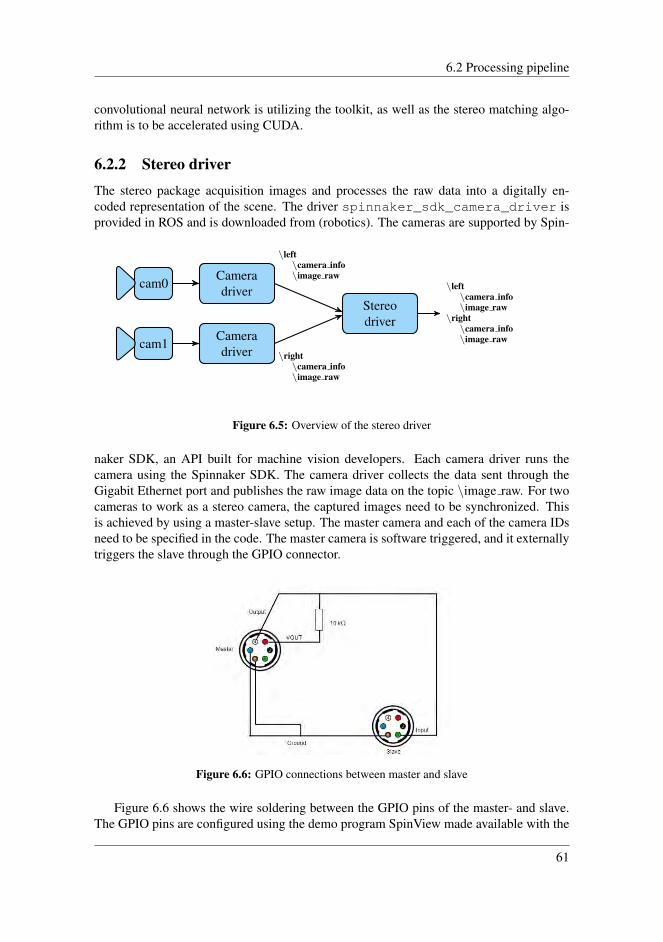
6.2 Processing pipeline
convolutional neural network is utilizing the toolkit, as well as the stereo matching algo-rithm is to be accelerated using CUDA.
6.2.2 Stereo driverThe stereo package acquisition images and processes the raw data into a digitally en-coded representation of the scene. The driver spinnaker_sdk_camera_driver isprovided in ROS and is downloaded from (robotics). The cameras are supported by Spin-
cam0
cam1
Cameradriver
Cameradriver
Stereodriver
\left\camera info\image raw
\right\camera info\image raw
\left\camera info\image raw
\right\camera info\image raw
Figure 6.5: Overview of the stereo driver
naker SDK, an API built for machine vision developers. Each camera driver runs thecamera using the Spinnaker SDK. The camera driver collects the data sent through theGigabit Ethernet port and publishes the raw image data on the topic \image raw. For twocameras to work as a stereo camera, the captured images need to be synchronized. Thisis achieved by using a master-slave setup. The master camera and each of the camera IDsneed to be specified in the code. The master camera is software triggered, and it externallytriggers the slave through the GPIO connector.
Figure 6.6: GPIO connections between master and slave
Figure 6.6 shows the wire soldering between the GPIO pins of the master- and slave.The GPIO pins are configured using the demo program SpinView made available with the
61

Chapter 6. System overview
Spinnaker SDK. The camera driver labels each image with a frame ID and a timestampaccording to ROS’s built-in clock ROS::Time. The timestamp and camera ID are passedto the stereo driver together with the calibration parameters on the topic \camera info.In the stereo driver node, two images are combined into a stereo pair. By synchronizingthe timestamps with a new identical timestamp, the stereo driver passes the images on forfurther processing.
6.2.3 3D reconstruction
While the stereo driver mainly acquisition images and set the stereo time stamp, the3D reconstruction package creates three-dimensional models from the image pair. Thepackage directly utilizes the theory in Chapter 2. The node Rectify is continuously run-
\left\camera info\image raw
\right\camera info\image raw
\stereo\points2
Rectify
Rectify
Disparitymap Point cloud
\left\camera info\image rect
\right\camera info\image rect
\stereo\disparity
\left\camera info
Figure 6.7: Overview of 3D Reconstruction
ning, concurrently subscribing to the topic image raw from the left and right camera,respectively. The node uses the metadata assigned on the topic camera info to removedistortion and for rectifying the co-calibrated cameras. Both the processes continuouslypublish rectified images, and the disparity nodelet subscribes to the topics. The disparitynodelet explicitly uses the timestamps from the stereo driver to correctly synchronize theimage pairs. The stereo matching algorithm produces a depth map that further is mappedto a point cloud. The nodelet Point Cloud combines the disparity map with the calibrationparameters to produce the point cloud.
6.2.4 Point cloud clustering
The package ptcloud clustering contains only one node, namely the PCL obstacle detec-tor. With the name-twin class, it filters and clusters the raw point cloud published fromthe 3D reconstruction package. For the ease of implementation, recording bagfiles, andtesting, it is included in a separate package. However, the node can advantageously beincluded in 3D reconstruction as a nodelet (inherit from the nodelet class). A nodelet willminimize memory usage, running multiple algorithms in the same process with zero-copytransport between algorithms.
62

6.3 Communication with milliAmpere
6.2.5 2D Object detectionA convolutional neural network recognizes and locates objects on the image plane. Thenode receives the left rectified image, and processes it to locates the 2D position of objects.The objects position in the image, the network’s confidence, and the type of object ispublished for acquiring the world position. The package utilizes CUDA for speeding upthe detection process.
6.2.6 CNN clusteringCNN-Clustering clusters the disparity map using the output from the 2D object detectionpackage. The disparity map is created from the left view of the stereo camera, whichis the same image fed to the convolutional neural network. The bounding box positionin the image extracts the area of interest in the disparity map. Message filter in ROSensures time synchronization between the disparity map and the bounding box predictions.By reconstruction, the world coordinates are extracted and published together with theprediction of the object type. The package publishes a message for each disparity mapcontaining a list of objects.
6.3 Communication with milliAmpereThe system in use on milliAmpere can be compiled in a graph, giving an overview ofthe code. The system overview is presented in Appendix F. The tree consists of nodes,topics, hardware, python modules, services, and namespaces used, and the communica-tion is illustrated with edges. This is the code currently running on the ferry, where forthis project the navigation data is the most pertinent. Due to the processing power, andmemory usage, the stereo system is running on a separate computer communicating withthe master on milliAmpere. The stereo system is connected through a Ethernet cable, forstable communication through topics.
6.3.1 Common world frameThe navigation data provided by milliAmpere is used to determine the world position ofobjects detected by the stereo camera. The system subscribes to the navigation data ofthe ferry, which provides the data needed to transform the detected object into the setworld frame. This places the vessel and the detected object in the same reference frame.The navigation data from milliAmpere and the detected objects by the stereo camera aresynchronized by their ROS-timestamps. Subsequently, the clustering packages transformsthe detected objects position into a North-East-Down (NED) reference frame. The stereocamera thus places objects in the local reference frame used by milliAmpere. The dataflow is illustrated in Figure 6.3.
As mentioned, the stereo camera was temporary placed on the ferry for testing pur-poses, making a calibrating of the stereo camera and the BODY frame unachievable. In-stead, the translation was measured by hand to the GPS sensors position on the ferry. Themeasured translation is tGPSc = [−1.86 0 0.29]>, given in meters. The translation of
63
Chapter 6. System overview
the GPS to BODY frame is already known; tbGPS = [0 − 0.975 2.33]. Due to the in-tended use of the system, meter precision of the stereo camera measurement is sufficient.The error due to hand measurement can be thus neglected. The axes of the coordinateframe of the stereo camera is defined differently, but is approximately aligned. Thus therotation of the stereo camera into the ferrys BODY frame is set to.
Rbc =
0 0 11 0 00 1 0
The transformation of the stereo cameras measurements is given by the matrices above,
and can further be rotated into the NED frame. This is done by the rotation Rnb . The
rotation is given bycosψcosθ − sinψ cosφ+ cosψ sin θ sinφ sinψ sinφ+ cosψ sin θ cosφsinψ cos θ cosψ cosφ+ sinψ sin θ sinφ − cosψ sin θ + sinψ sin θ cosφ− sin θ cos θ sinφ cos θ cosφ
where φ, θ and ψ is the roll, pitch, and yaw of the vessel, respectively (Fossen, 2011). Astesting on milliAmpere is performed under calm sea, three DOF is assumed, i.e., pitch androll is negligible. The rotation is thus simplified to
Rnb =
cosψ − sinψ 0sinψ cosψ 0
0 0 1
where ψ is the heading. The heading is provided by the navigation system on milliAmpere.The detected objects position is know given in NED coordinates in the ferrys BODY frame.
To give the detected objects in a world frame, the geodetic coordinates of milliAmpereare transformed into the NED frame set in the operational area. The world position ofmilliAmpere is given in geodetic coordinates using latitude as the World Geodetic System84 reference ellipsoid (WGS-84). The coordinates is thus given in latitude µ, longitudel and elevation h. Before transforming to NED coordinates a transformation to Earth-Centered, Earth-Fixed (ECEF) coordinates is performed byxeye
ze
=
(N + h) cosµ cos l(N + h) cosµ sin l
(r2pr2eN + h) sinµ
where re and rp is the equatorial and polar axis radius of the ellipsoid (Fossen, 2011).Their values are given by WGS-84. N is the radius of the curvature in the prime verticalof the ellipsoid and can be calculated by
N =r2e√
r2e cos2 µ+ r2e sin2 µ
64
6.3 Communication with milliAmpere
The NED frame can now be found byxnynzn
=
− sinµ0 cos l0 − sinµ0 sin l0 cosµ0
− sin l0 cos l0 0− cosµ0 cos l0 − cosµ0 sin l0 − sinµ0
xe,b − xe,0ye,b − ye,0ze,b − ze,0
where xe,0, ye,0 and ze,0 and l0 and µ0 are the ECEF and geodetic coordinates of the originof the NED frame. xe,b, ye,b and ze,b are the ECEF coordinates of the origin of the BODYframe. Points in the body frame can now be transformed to NED frame by Rn
b and tnb .The translation tnb is the world position of milliAmpere in the NED frame.
65

Chapter 6. System overview
66
Chapter 7Object detection
Object detection and localization are essential parts of a tracking system. The classificationof objects is also helpful, especially for a ship that needs to follow legislation at sea. Fora stereo camera, this means that the captured images need to be post-processed to obtainworld coordinates of objects in the scene. In this chapter, the methods and algorithmsused in the proposed system are presented. As well as an overview of some uncertaintiespresent in the stereo system.
7.1 Uncertainty in the stereo systemFor the system to perform a correct localization of objects, it has to rely on an accuratecalibration. The most accurate calibration in Chapter 5 is the 20meters calibration. The pa-rameters performed overall with the highest accuracy. However, as they were determinedon solid ground, with large scale buildings, a re-estimate of the accuracy for use at sea isdesirable. By analyzing the obtained parameters, an estimate of the expected accuracy isgiven based on the operating environment. The extrinsic parameters of the calibration at20 meters are given in equation (7.1).
R20 =[−0.0439 −1.7265 0.0261
], t20 =
[−1.860 0.0095 −0.025
](7.1)
7.1.1 Reprojection errorThe obtained calibration parameters (7.1) had an average reprojection error of 0.3091 pix-els in the calibration process. This is the mean accuracy; hence the error can be higher atsome parts of the image. The erroneousness means the 3D reconstruction will be slightlybiased, but typically one assumes that these small errors do not cause problems for stereomatching (Hirschmuller and Gehrig, 2009). However, most literature uses and evaluatestereo accuracy on shorter distances. Figure 7.1a illustrate the relationship of the disparityand its corresponding depth estimate for the 20 meter-graph, extracted from Figure 5.2.
67

Chapter 7. Object detection
The depth error one expects from an error of one pixel in the disparity is shown in figure7.1b. Table 7.1 summarizes the depth error on different distances from a given pixel-error.The pixel error is determined by computing in the slope of one pixel.
10 20 30 40 50 60 70 80 90 100
Disparity (pixels)
0
50
100
150
200
250
Estim
ate
d D
epth
(m
)
Estimated Depth from given pixel disparity
(a) Depth on given pixel disparity
10 20 30 40 50 60 70 80 90 100
Disparity (pixels)
-25
-20
-15
-10
-5
0
Depth
err
or
(m)
Depth error resulting from a deviation of one pixel in the disparity
(b) Depth uncertainty on given pixel disparity
Figure 7.1: Depth estimate for a given disparity and the error estimate for a one pixel deviation inthe disparity (Baseline = 1.860m)
Real world-depth Disparity Depth error
[1 pixel error]10 m 229.3 ± 0.044m20 m 114.7 ± 0.175m30 m 76,5 ± 0.392m40 m 57.3 ± 0.699m50 m 45.9 ± 1.091m60 m 38.2 ± 1.572m70 m 32.8 ± 2.138m80 m 28.7 ± 2.794m90 m 25.5 ± 3.541m
100 m 22.9 ± 4.373m110 m 20.9 ± 5.275m120 m 19.1 ± 6.287m130 m 17.7 ± 7.362m140 m 16.4 ± 8.527m150 m 15.3 ± 9.797m
Table 7.1: Expected error based on pixels and baseline
68
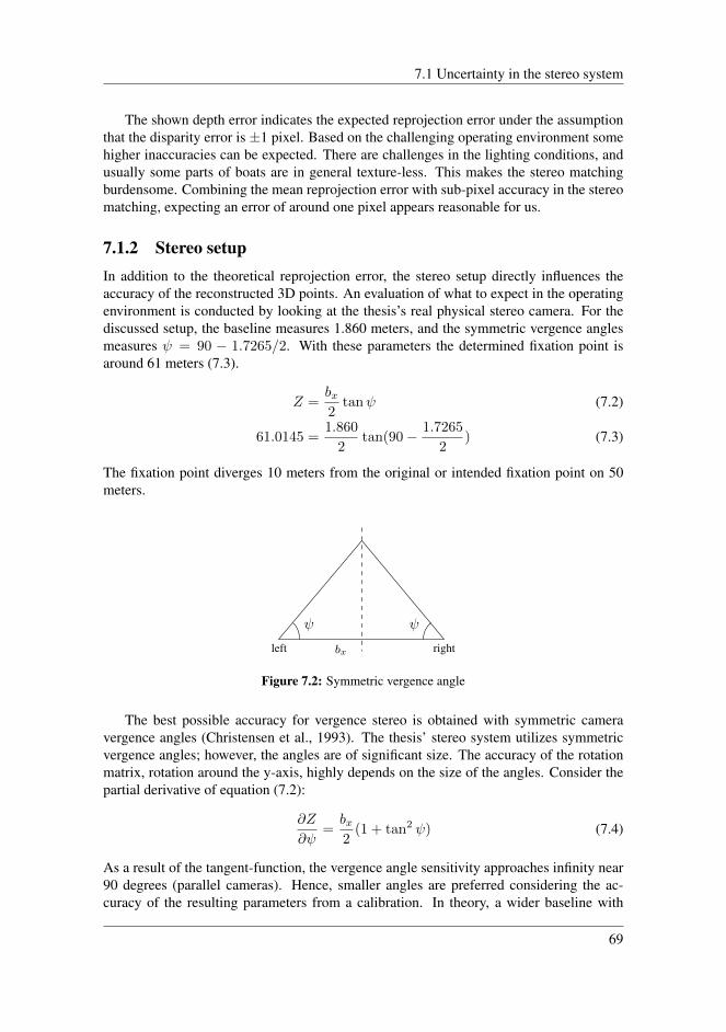
7.1 Uncertainty in the stereo system
The shown depth error indicates the expected reprojection error under the assumptionthat the disparity error is ±1 pixel. Based on the challenging operating environment somehigher inaccuracies can be expected. There are challenges in the lighting conditions, andusually some parts of boats are in general texture-less. This makes the stereo matchingburdensome. Combining the mean reprojection error with sub-pixel accuracy in the stereomatching, expecting an error of around one pixel appears reasonable for us.
7.1.2 Stereo setupIn addition to the theoretical reprojection error, the stereo setup directly influences theaccuracy of the reconstructed 3D points. An evaluation of what to expect in the operatingenvironment is conducted by looking at the thesis’s real physical stereo camera. For thediscussed setup, the baseline measures 1.860 meters, and the symmetric vergence anglesmeasures ψ = 90 − 1.7265/2. With these parameters the determined fixation point isaround 61 meters (7.3).
Z =bx2
tanψ (7.2)
61.0145 =1.860
2tan(90− 1.7265
2) (7.3)
The fixation point diverges 10 meters from the original or intended fixation point on 50meters.
left rightbx
ψ ψ
Figure 7.2: Symmetric vergence angle
The best possible accuracy for vergence stereo is obtained with symmetric cameravergence angles (Christensen et al., 1993). The thesis’ stereo system utilizes symmetricvergence angles; however, the angles are of significant size. The accuracy of the rotationmatrix, rotation around the y-axis, highly depends on the size of the angles. Consider thepartial derivative of equation (7.2):
∂Z
∂ψ=bx2
(1 + tan2 ψ) (7.4)
As a result of the tangent-function, the vergence angle sensitivity approaches infinity near90 degrees (parallel cameras). Hence, smaller angles are preferred considering the ac-curacy of the resulting parameters from a calibration. In theory, a wider baseline with
69

Chapter 7. Object detection
a smaller vergence angle would enhance the calibration accuracy on the given fixationpoint. However, the baseline in use is the largest baseline available to implement on theferry, thus an additional source of error.
88.6 88.7 88.8 88.9 89 89.1 89.2 89.3 89.4
Vergence angle (deg)
40
50
60
70
80
90
De
pth
(m
)
Depth versus vergence angle (Baseline = 1.860m)
(a) Depth estimate on given vergence angle
80 82 84 86 88 90
Vergence angle (deg)
0
50
100
150
200
250
300
350
Change in d
epth
(m
)
Change in depth versus vergence angle (Baseline = 1.860m)
(b) Depth uncertainty given a change in vergence angle of 0.01 degrees
Figure 7.3: Depth estimate for a given vergence angle, and the error estimate for a deviation of 0.01degrees in vergence angle
From the plots in Figure 7.3, one can see how sensitive the setup is to changes inangling. Error in angling can arise either from wrong calibration estimates or from externalsources that reluctantly change the angling during the system’s lifetime.
Irrespective of the angling, the baseline and focal length directly influence the uncer-tainty of the depth estimates. From equation 2.10, the uncertainty of the baseline and focallength will introduce approximately the same amount of uncertainty in the depth estimates.The translation in x-direction diverges 6 centimeters from the expected value, while no va-lidity exists for the focal length. Therefore the average error from Chapter 5 is used as afoundation for uncertainty. The depth error from the test scenes yields to be approximatelyconstant for the 20m calibration. Subtracting the expected one pixel error from Table 7.1can be interpreted as an estimate of the overall uncertainties of the real stereo setup.
Distance Actualtest-scene error
Expectedreprojection error
30 m 1.23 m 0.392 m40 m 0.94 m 0.699 m50 m 1.65 m 1.091 m70 m 1.32 m 2.138 m90 m 1.25 m 3.541 m
Table 7.2: Error from the real physical stereo camera, with the expected theoretical error
70
7.2 The disparity map algorithm
In Table 7.2, the reprojection errors are shown that were extracted from the test sce-narios. By comparing the measured errors with the expected theoretical error, the experi-mental error turned out to be higher than in our theoretical consideration. The theoreticalassumptions were more optimistic about the possible setup and measurement deviations. Itcan be caused by several reasons which finally accumulate to a higher error. This includeshigher errors in the estimation of the baseline and the relative orientation of the cameras,but also higher errors in the estimation of the matching position of corresponding points.
The uncertainty of the physical stereo camera is expected to yield an even higher errorfor testing in the operating environment than in Table 7.2. The test scene is a bit un-reliable as it contains an enormous building similar to the calibration scene. Besides, itutilizes semi-global matching which is shown to be more precise than our chosen real-time disparity-algorithm (described in the subsequent section). Thus, assuming an error ofabout 2-3 pixels seems to be more appropriate for the real physical stereo camera.
The finding from this subsection estimates the reprojection error to be highly depen-dent on the operating distance. As well, uncertainties in estimating the stereo setup have anegative impact on the overall accuracy. Therefore, higher uncertainty is to be expected. Amore precise estimation of the error is to be determined by trial and error in the operatingenvironment.
7.2 The disparity map algorithmWhen processing images from a stereo camera, the corresponding pixels in the two imagesneed to be matched to obtain depth information. Based on the evaluation of matchingalgorithms presented in the specialization project by Olsen (2020), a simple correlation-based method is preferred. Due to real-time computation, the chosen algorithm categorizesas a local method with a low computational cost.
7.2.1 Sum of Absolute DifferenceSum of Absolute Difference (SAD) is known for its simplicity and low execution time. Itis one of the simplest methods for matching corresponding pixels but still has an advantagedue to few memory requirements. (Thaher and Hussein, 2014)
The main idea is to find matching pixels by exploiting the neighborhood around apixel. The neighborhood is a predefined block, and when used on rectified images, asuitable match is found on the same horizontal axis in the second image. The search startsin the same location as the reference block and moves along the horizontal line. A matchis defined as the block with the most similarity. Similarity is computed by a cost function,measuring the absolute intensity difference between two selected neighborhoods.
CSAD(d) =∑
(u,v)∈Wm
|IL(u, v)− IR(u− d, v)| (7.5)
The cost function (7.5) measures absolute similarity, and the block with the minimumcost is considered a match. The intensity of pixel (u − d, v) in the right image IR issubtracted from the reference intensity in the left image IL. The cost is summed over the
71
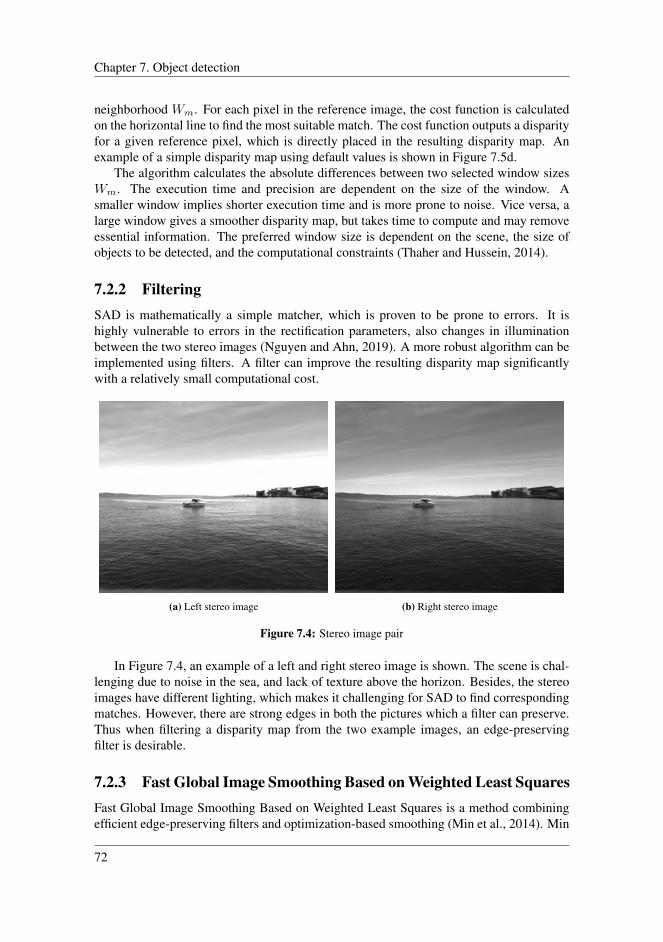
Chapter 7. Object detection
neighborhood Wm. For each pixel in the reference image, the cost function is calculatedon the horizontal line to find the most suitable match. The cost function outputs a disparityfor a given reference pixel, which is directly placed in the resulting disparity map. Anexample of a simple disparity map using default values is shown in Figure 7.5d.
The algorithm calculates the absolute differences between two selected window sizesWm. The execution time and precision are dependent on the size of the window. Asmaller window implies shorter execution time and is more prone to noise. Vice versa, alarge window gives a smoother disparity map, but takes time to compute and may removeessential information. The preferred window size is dependent on the scene, the size ofobjects to be detected, and the computational constraints (Thaher and Hussein, 2014).
7.2.2 FilteringSAD is mathematically a simple matcher, which is proven to be prone to errors. It ishighly vulnerable to errors in the rectification parameters, also changes in illuminationbetween the two stereo images (Nguyen and Ahn, 2019). A more robust algorithm can beimplemented using filters. A filter can improve the resulting disparity map significantlywith a relatively small computational cost.
(a) Left stereo image (b) Right stereo image
Figure 7.4: Stereo image pair
In Figure 7.4, an example of a left and right stereo image is shown. The scene is chal-lenging due to noise in the sea, and lack of texture above the horizon. Besides, the stereoimages have different lighting, which makes it challenging for SAD to find correspondingmatches. However, there are strong edges in both the pictures which a filter can preserve.Thus when filtering a disparity map from the two example images, an edge-preservingfilter is desirable.
7.2.3 Fast Global Image Smoothing Based on Weighted Least SquaresFast Global Image Smoothing Based on Weighted Least Squares is a method combiningefficient edge-preserving filters and optimization-based smoothing (Min et al., 2014). Min
72
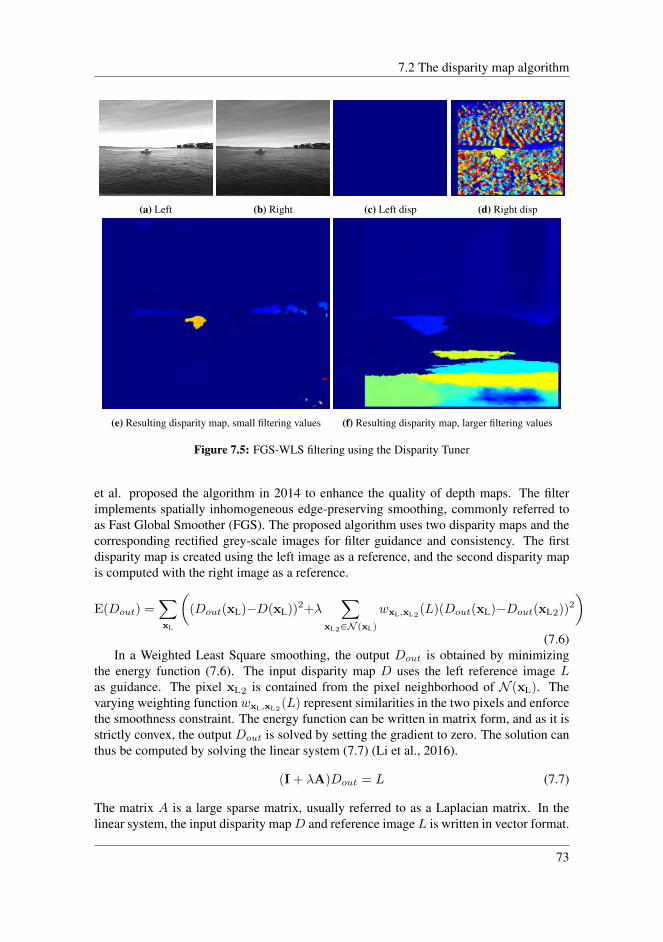
7.2 The disparity map algorithm
(a) Left (b) Right (c) Left disp (d) Right disp
(e) Resulting disparity map, small filtering values (f) Resulting disparity map, larger filtering values
Figure 7.5: FGS-WLS filtering using the Disparity Tuner
et al. proposed the algorithm in 2014 to enhance the quality of depth maps. The filterimplements spatially inhomogeneous edge-preserving smoothing, commonly referred toas Fast Global Smoother (FGS). The proposed algorithm uses two disparity maps and thecorresponding rectified grey-scale images for filter guidance and consistency. The firstdisparity map is created using the left image as a reference, and the second disparity mapis computed with the right image as a reference.
E(Dout) =∑xL
((Dout(xL)−D(xL))2+λ
∑xL2∈N (xL)
wxL,xL2(L)(Dout(xL)−Dout(xL2))2
)(7.6)
In a Weighted Least Square smoothing, the output Dout is obtained by minimizingthe energy function (7.6). The input disparity map D uses the left reference image Las guidance. The pixel xL2 is contained from the pixel neighborhood of N (xL). Thevarying weighting function wxL,xL2
(L) represent similarities in the two pixels and enforcethe smoothness constraint. The energy function can be written in matrix form, and as it isstrictly convex, the output Dout is solved by setting the gradient to zero. The solution canthus be computed by solving the linear system (7.7) (Li et al., 2016).
(I + λA)Dout = L (7.7)
The matrix A is a large sparse matrix, usually referred to as a Laplacian matrix. In thelinear system, the input disparity mapD and reference image L is written in vector format.
73

Chapter 7. Object detection
For efficiently solving the equation (7.7), one-dimensional Fast Global Smoothing isutilized. The key idea is that the matrix A is a tridiagonal matrix in a one-dimensionalsystem. For images in grey-scale, one dimension means horizontal or vertical inputs. Bysolving a series of multiple linear equations over the total image, the exact solution ofequation (7.6) can be solved. The one-dimensional linear equations are solved by theGaussian elimination algorithm (Golub and Van Loan, 2013) in a recursive manner. Byrepeating the linear equation over horizontal lines in the image, the result is the minimumsolution of (7.6).
In Figure 7.5, the two guidance images are displayed together with the two disparityimages by SAD. Figure 7.5e and 7.5f shows the resulting disparity map from executingthe Fast Global Smoothing based on WLS filtering.
7.2.4 Implementation
1 //Creating a disparity map from two rectified images2 void DisparityNodelet::imageCallBack(left_rectified_image,
right_rectified_image, calibration_params)3
4 convert images to opencv lib5 downscale images //speed up the execution, optional6
7 compute left disparity map8 compute right disparity map9 WLSfilter(left image, left disparitymap, right image,
right disparity map)10
11 upscale image //optional12
13 Adjust offset in principal point14
15 Convert to ros msg16 publish(disparityMap)
Listing 7.1: Create disparity map
The algorithm is notated in pseudo-code in Listing 7.1. The image callback is a ROS-function which is executed every time a new image is published to a rectification-topic. Itlistens to camera calibration parameters and the left- and right rectified images. Whenevertwo images are published, the function is called, and it checks that the timestamp of theimages is equal. The stereo image pairs are further converted to use the OpenCV imagelibrary. The first disparity map is computed using SAD with the left image as the reference.The second disparity map uses the right image as a reference. Both matching pixels withthe fast and efficient stereo matching algorithm based on Konolige (Konolige, 1998). FastGlobal Smoothing combines the two disparity maps with both the rectified images forpreserving edges and smoothing the result. The resulting disparity map is subsequentlypublished to a topic for later creating the world position for regions of interest.
74
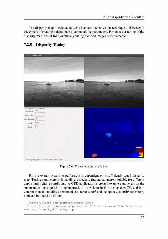
7.2 The disparity map algorithm
The disparity map is calculated using standard stereo vision techniques. However, atricky part of creating a depth map is tuning all the parameters. For an easier tuning of thedisparity map, a GUI for dynamically tuning rectified images is implemented.
7.2.5 Disparity Tuning
Figure 7.6: The stereo tuner application
For the overall system to perform, it is dependent on a sufficiently tuned disparitymap. Tuning parameters is demanding, especially finding parameters suitable for differentdepths and lighting conditions. A GTK application is created to tune parameters on thestereo matching algorithm implemented. It is written in C++ using openCV, and is acombination and modified version of the stereo-tuner1 and the opencv contrib2 repository,both can be found on Github.
1https://github.com/guimeira/stereo-tuner2https://github.com/opencv/opencv_contrib/blob/master/modules/ximgproc/
samples/disparity_filtering.cpp
75

Chapter 7. Object detection
The application has a graphical interface where parameters can be changed dynami-cally. A screenshot of the application is displayed in Figure 7.6. The two upper imagesare the rectified stereo images from the left and right camera, respectively, while the lowerright image is the resulting disparity map. Only the parameters influencing the disparitymap is chosen in the application. This is the block size for SAD and the disparity range forsearching for matches on the horizontal line. For the filter, sigma and lambda are includedfor tuning. Lambda, λ in (7.6), defines the amount of regularization during filtering. Largevalues will adhere to the disparity map edges closer to the guidance image. Sigma definesthe sensitivity of the filtering. Larger values smooth the resulting image but may misssome of the corners.
7.3 2D Object Detection with YOLOThe detection of objects in an image is twofold. It consists of locating the exact positionof objects in an image, and subsequently classify each object. YOLOv3 (Redmon andFarhadi, 2018) is a fast and accurate real-time detection system. In the overall system,YOLOv3 is implemented to locate objects of interest in the left stereo image. By combin-ing the disparity map found in Section 7.2 with a trained network, it can output positionsof detected objects in world coordinates.
YOLO is a single convolutional neural network, engineered to detect patterns in im-ages. It is a type of neural network, a special kind of computer algorithms.
Neural Networks
A neural network is inspired by the knowledge of the inner workings of the human brain.It consists of perceptrons, which is a mathematical model of a biological neuron. Thenodes are connected to one another to model pattern recognition capabilities. A network ismade up of layers, and they can be trained to perform specific tasks like image recognition,image classification, and image captioning.
A neural network comprises one input layer, one output layer, and at least one hiddenlayer. Figure 7.7 illustrates a simple three-layer neural network consisting of only onehidden layer. Each input of a neuron is multiplied with a weight wi. The weighted sum, a,of a neuron is given in (7.8).
a =
n∑i=1
wix+ b (7.8)
The signal or value xj represents the input, and b is applied to allow for a constant bias tothe neuron. The neuron generates an output when the weighted sum exceeds an activationthreshold set by an activation function. The parameters of the weights and biases are setduring training. When training a neural network, the parameters are tuned to find thedesired output. (Krenker et al., 2011)
Convolutional Neural Networks
Convolutional neural networks, CNN, is a special case of neural networks. CNN’s aremade of mostly convolutional layers, which are designed for having images as inputs. The
76
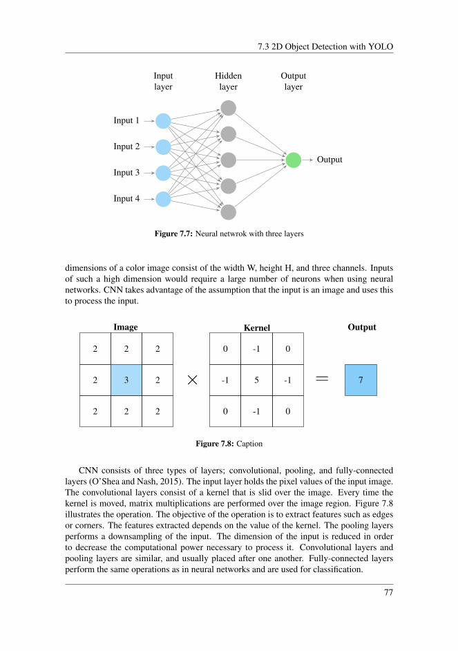
7.3 2D Object Detection with YOLO
Input 1
Input 2
Input 3
Input 4
Output
Hiddenlayer
Inputlayer
Outputlayer
Figure 7.7: Neural netwrok with three layers
dimensions of a color image consist of the width W, height H, and three channels. Inputsof such a high dimension would require a large number of neurons when using neuralnetworks. CNN takes advantage of the assumption that the input is an image and uses thisto process the input.
2 2 2
2 3 2
2 2 2
Image
×
0 -1 0
-1 5 -1
0 -1 0
Kernel
= 7
Output
Figure 7.8: Caption
CNN consists of three types of layers; convolutional, pooling, and fully-connectedlayers (O’Shea and Nash, 2015). The input layer holds the pixel values of the input image.The convolutional layers consist of a kernel that is slid over the image. Every time thekernel is moved, matrix multiplications are performed over the image region. Figure 7.8illustrates the operation. The objective of the operation is to extract features such as edgesor corners. The features extracted depends on the value of the kernel. The pooling layersperforms a downsampling of the input. The dimension of the input is reduced in orderto decrease the computational power necessary to process it. Convolutional layers andpooling layers are similar, and usually placed after one another. Fully-connected layersperform the same operations as in neural networks and are used for classification.
77
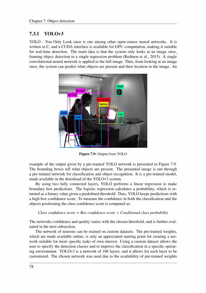
Chapter 7. Object detection
7.3.1 YOLOv3YOLO - You Only Look once is one among other open-source neural networks. It iswritten in C, and a CUDA interface is available for GPU computation, making it suitablefor real-time detection. The main idea is that the system only looks at an image once,framing object detection to a single regression problem (Redmon et al., 2015). A singleconvolutional neural network is applied to the full image. Thus, from looking at an imageonce, the system can predict what objects are present and their location in the image. An
Figure 7.9: Output from YOLO
example of the output given by a pre-trained YOLO network is presented in Figure 7.9.The bounding boxes tell what objects are present. The presented image is run througha pre-trained network for classification and object recognition. It is a pre-trained model,made available in the download of the YOLOv3 system.
By using two fully connected layers, YOLO performs a linear regression to makeboundary box predictions. The logistic regression calculates a probability, which is re-turned as a binary value given a predefined threshold. Thus, YOLO keeps predictions witha high box confidence score. To measure the confidence in both the classification and theobjects positioning the class confidence score is computed as:
Class confidence score = Box confidence score× Conditional class probability
The networks confidence and quality varies with the chosen threshold, and is further eval-uated in the next subsection.
The network of neurons can be trained on custom datasets. The pre-trained weights,which are made available online, is only an appreciated starting point for creating a net-work suitable for more specific tasks of own interest. Using a custom dataset allows theuser to specify the detection classes and to improve the classification in a specific operat-ing environment. YOLOv3 is a network of 106 layers, and it allows for each layer to becustomized. The chosen network was used due to the availability of pre-trained weights
78

7.3 2D Object Detection with YOLO
developed during a Master thesis project by Grini (2019) at NTNU. The framework istrained for detecting boats in images. The dataset consists of images captured in andaround the fjords in Trondheim, combined with some online datasets.
The network is implemented using a pre-exisiting ros-package3, and combined with thenew weighs. To accelerate the execution the package is utilized by installing the NvidiaCUDA Toolkit 10.2. This boosts the network to use parallel computing for real-time per-formance. A pre-trained network requires a threshold in percentage for classifying ob-jects. The training dataset in its whole and the confidence threshold of the application isunknown. For this reason, an analysis of the quality is conducted before taking it to use.
7.3.2 Precision recall curvePrecision-Recall metric is a useful measure to evaluate the classifiers output quality. Byusing different probability thresholds, the curve summarizes the trade-off between the truepositive rate and the positive predictive value for the network. Precision Pn (7.9) definesthe true positive rate for the threshold n, and recall Rn (7.10) the positive predicted valuefor the threshold n. With the given weights in the thesis, the classifier is binary, i.e., boator not boat.
Pn =TP
TP + FP(7.9)
Rn =TP
TP + FN(7.10)
Both the functions consist of the abbreviations in (7.11).
TP = True positive: boats correctly classified
FP = False positive: miss-classifications (7.11)FN = False negative: boats not classified
High precision shows that the classifier is accurate and does not label wrong objectsas boats. The recall score is the ability of the classifier to find all the boats in the picture.Lowering the threshold of the neural network may increase the precision’s denominator byincreasing the number of results returned. The denominator of the recall does not dependon the classifiers threshold, implying that lowering the threshold will mostly increase therecall. If the recall leaves unchanged while changing the threshold, the precision mayfluctuate.
The values are usually comprised in a confusion matrix, defined in Table 7.3 The last
PredictedPositive Negative
Actual Positive TP FNNegative FP TN
Table 7.3: Confusion matrix
3https://github.com/leggedrobotics/darknet_ros
79

Chapter 7. Object detection
value, TN, is defined as no boats present nor detected. When detecting and classifyingobjects in a picture, it makes no to little sense using TN, because a negative class does notexist. The negative class is defined as parts of the image not including boats.
Computing the curve
To evaluate the accuracy of the network a ground truth dataset was labeled. The imagesare taken in the test area outside the port of Brattøra. The dataset and the graphical userinterface are presented in Appendix D. The labeled images are the ground truth, implying asquared PRC with both precision and recall equal to zero. It is the same boat, just capturedat various distances and with different headings. In theory, a perfectly trained networkshould be able to detect the same boat with about the same confidence and similar sizedboxes.
PredictedPositive Negative
Actual Positive 483 0Negative 0 -
Table 7.4: Ground-truth Confusion matrix
IoU =Area of Overlap
Area of Union=
The ground truth bounding boxes are compared with the bounding boxes predictedby YOLO. To get a comparison, the Intersect over Union, IoU, is calculated. The pre-dicted bounding box is a match if it shares the same label as the ground-truth and hasconfidence- and IoU- value above the given thresholds. Only one predicted bounding boxcan be assigned to the ground truth to avoid multiple detections of the same object. Thepseudocode of the implementation is given in Listing 7.2. The implementation is given inthe GitHub-repository explained in Appendix C. The PRC is calculated for each IoU- andYOLO-threshold, of all the images in the dataset.
1 for each IoU-threshold2 for each YOLO-threshold
80

7.3 2D Object Detection with YOLO
3
4 sort detection-results by decreasing confidence5 for each detection confidence >= YOLO-threshold6 for each class7 assign detected box to ground-truth object8 if IoU >= IoU-threshold9 TP ++
10 else11 FP ++12
13 Precision = TP/(TP+FP)14 Recall = TP/ (number of ground truth objects)15 Plot curve
Listing 7.2: Pseudocode plot PRC
Figure 7.10: Precision Recall Curve
The resulting plot is presented in Figure 7.10. Each colored line represents the givenIoU-threshold used for counting the True Positive detections. The dots represent a giventhreshold for the YOLO-network. The YOLO-threshold is plotted from 0 to 1 with a stepsize of 0.05. The YOLO-threshold of 0.95 and 0.005 of each curve are given in the topleft and lower right corners, respectively. The graph with the largest area under the curvehas IoU= 0.10%. The node giving the largest possible area is computed with a YOLO-threshold of 0.45. The associated confusion matrix is given below and corresponds to a
81
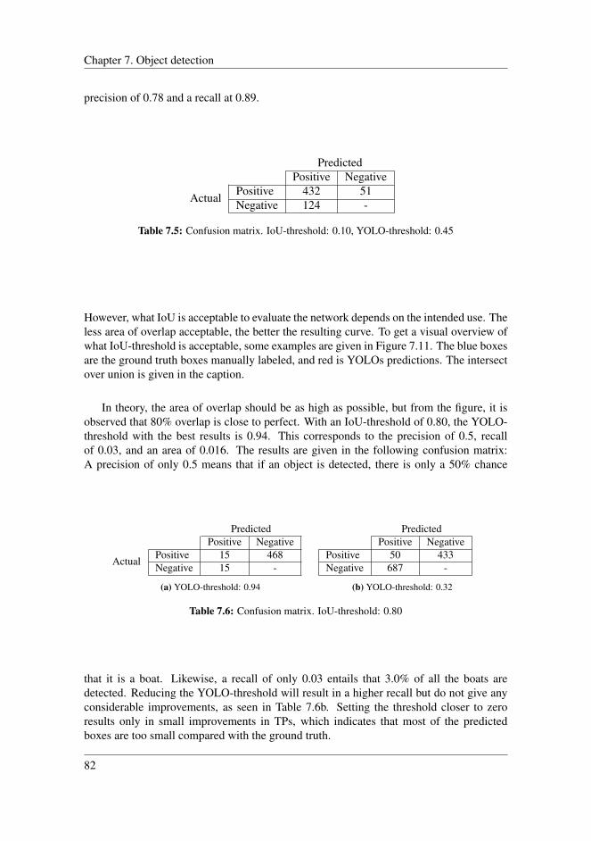
Chapter 7. Object detection
precision of 0.78 and a recall at 0.89.
PredictedPositive Negative
Actual Positive 432 51Negative 124 -
Table 7.5: Confusion matrix. IoU-threshold: 0.10, YOLO-threshold: 0.45
However, what IoU is acceptable to evaluate the network depends on the intended use. Theless area of overlap acceptable, the better the resulting curve. To get a visual overview ofwhat IoU-threshold is acceptable, some examples are given in Figure 7.11. The blue boxesare the ground truth boxes manually labeled, and red is YOLOs predictions. The intersectover union is given in the caption.
In theory, the area of overlap should be as high as possible, but from the figure, it isobserved that 80% overlap is close to perfect. With an IoU-threshold of 0.80, the YOLO-threshold with the best results is 0.94. This corresponds to the precision of 0.5, recallof 0.03, and an area of 0.016. The results are given in the following confusion matrix:A precision of only 0.5 means that if an object is detected, there is only a 50% chance
PredictedPositive Negative
ActualPositive 15 468Negative 15 -
(a) YOLO-threshold: 0.94
PredictedPositive Negative
Positive 50 433Negative 687 -
(b) YOLO-threshold: 0.32
Table 7.6: Confusion matrix. IoU-threshold: 0.80
that it is a boat. Likewise, a recall of only 0.03 entails that 3.0% of all the boats aredetected. Reducing the YOLO-threshold will result in a higher recall but do not give anyconsiderable improvements, as seen in Table 7.6b. Setting the threshold closer to zeroresults only in small improvements in TPs, which indicates that most of the predictedboxes are too small compared with the ground truth.
82
7.3 2D Object Detection with YOLO
(a) IoU=9% (b) IoU=14% (c) IoU=14% (d) IoU=18%
(e) IoU=20% (f) IoU=23% (g) IoU=25% (h) IoU=29%
(i) IoU=35% (j) IoU=35% (k) IoU=38% (l) IoU=41%
(m) IoU=62% (n) IoU=67% (o) IoU=70% (p) IoU=73%
(q) IoU=80% (r) IoU=86% (s) IoU=90% (t) IoU=91%
Figure 7.11: Example of the IoU with ground truth in blue and YOLO predictions in red
83

Chapter 7. Object detection
Looking at the pictures in Figure 7.11, one can estimate the preferred IoU-thresholdfor the application. With IoU less than 0.2, the predicted bounding boxes seem to detecttoo much of the surroundings. However, increasing the threshold above 0.2, most of thepredicted bounding boxes primarily detect the boat. The bounding boxes are too smallcompared to the ground truth, but parts of the boat are detected. The network is imple-mented together with the disparity map to get depth estimates. By using a disparity withsome smoothing, the same depth values will yield for every pixel where the boat is present.Thus, YOLO only needs to detect a small part of the boat for the system to extract it fromthe disparity map and reconstruct its 3D position.
(a) 1 (b) 2 (c) 3 (d) 4
(e) 5 (f) 6 (g) 7 (h) 8
(i) 9 (j) 10 (k) 11 (l) 12
Figure 7.12: Example of predictions in a time sequence, images in chronological order. YOLO-threshold: 0.44
For IoU-threshold of 0.2, the results from differing the YOLO-thresholds is writtenin the table in Appendix E. From the table, the YOLO-threshold giving the largest areais 0.44. The confusion matrix is given in Table 7.7. With a recall of 89%, the networkstill misses out on 52 out of 483 boats in the images. Not detecting 11% of the boats canbe critical for an autonomous navigation system, increasing the likelihood of a collision.However, if the probability for detecting a boat is independent and 89%, setting the framerate to about 10 will ensure enough TPs to establish the presents of a boat. Looking atthe dataset in Figure 7.12 and 7.13 comparing two time-sequences of images, one can
84
7.3 2D Object Detection with YOLO
observe that the probability of detecting a boat is indeed dependent on the scene. In thefirst time-sequence, YOLO detects 25% of the boats, while in the second it detects 100%of the boats. Thus, as the system is meant for collision avoidance, the YOLO-threshold
PredictedPositive Negative
Actual Positive 431 52Negative 146 -
Table 7.7: Confusion matrix. IoU-threshold: 0.20. YOLO-threshold: 0.44
is decreased to increase the recall. Even though this implies decreasing the precision,detecting all boats is of higher importance. From the table in Appendix E, a recall of 1 canbe obtained with a threshold of 0.2. The confusion matrix is given in Table 7.8, with threeadditional thresholds of interest.
PredictedPositive Negative
483 0525 -
(a) YOLO-threshold: 0.20
PredictedPositive Negative
482 1368 -
(b) YOLO-threshold: 0.26
PredictedPositive Negative
480 3350 -
(c) YOLO-threshold: 0.27
PredictedPositive Negative
471 12256 -
(d) YOLO-threshold: 0.33
Table 7.8: Confusion matrix. IoU-threshold: 0.20
The optimal threshold is a matter of the intended use of the system. In the case ofobject detection, to be able to trust the output, a well-trained network would be preferred.As the available YOLO-weights struggle with detecting the same boat, a higher recall ispreferred to detect as many boats as possible. A higher recall will increase the number ofFPs. A miss-classification of 525 images is not that bad considering the wrong match inFigure 7.13. In the case of multiple matches, the one with the lowest confidence score ischosen as the TP, the other as FP. In total, around half of the FPs are because of multiplematches on the same boat. However, YOLO tends to miss-classify the same buildings asboats, which implies that the probabilities are not independent. Therefore FPs should beminimized. Regardless, the thresholds of 0.26, 0.27, and 0.33 are added to see the changein FPs and FNs. Increasing the threshold from 0.20 to 0.26 shows quite an improvement.The FP is decreased with 157 boats, and the network only misses one boat.
85

Chapter 7. Object detection
(a) 1 (b) 2 (c) 3 (d) 4
(e) 5 (f) 6 (g) 7 (h) 8
(i) 9 (j) 10 (k) 11 (l) 12
(m) 13 (n) 14 (o) 15 (p) 16
(q) 17 (r) 18 (s) 19 (t) 20
Figure 7.13: Example of predictions in a time sequence, images in chronological order. YOLO-threshold 0.20
The threshold chosen in the thesis is 0.26. In the ground truth dataset, the network only
86
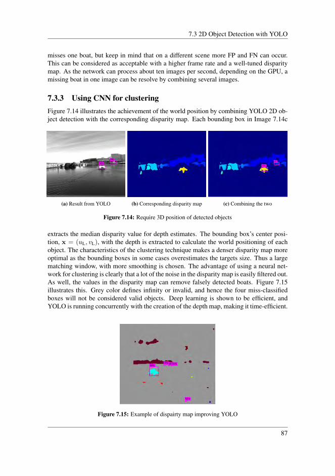
7.3 2D Object Detection with YOLO
misses one boat, but keep in mind that on a different scene more FP and FN can occur.This can be considered as acceptable with a higher frame rate and a well-tuned disparitymap. As the network can process about ten images per second, depending on the GPU, amissing boat in one image can be resolve by combining several images.
7.3.3 Using CNN for clusteringFigure 7.14 illustrates the achievement of the world position by combining YOLO 2D ob-ject detection with the corresponding disparity map. Each bounding box in Image 7.14c
(a) Result from YOLO (b) Corresponding disparity map (c) Combining the two
Figure 7.14: Require 3D position of detected objects
extracts the median disparity value for depth estimates. The bounding box’s center posi-tion, x = (uL, vL), with the depth is extracted to calculate the world positioning of eachobject. The characteristics of the clustering technique makes a denser disparity map moreoptimal as the bounding boxes in some cases overestimates the targets size. Thus a largematching window, with more smoothing is chosen. The advantage of using a neural net-work for clustering is clearly that a lot of the noise in the disparity map is easily filtered out.As well, the values in the disparity map can remove falsely detected boats. Figure 7.15illustrates this. Grey color defines infinity or invalid, and hence the four miss-classifiedboxes will not be considered valid objects. Deep learning is shown to be efficient, andYOLO is running concurrently with the creation of the depth map, making it time-efficient.
Figure 7.15: Example of dispairty map improving YOLO
87

Chapter 7. Object detection
7.4 Point Cloud ClusteringThe images captured by a stereo camera are rectified and utilized in the creation of adisparity map. A disparity map contains depth information needed to reconstruct the cap-tured scene in 3D. In both the disparity map and the reconstructed point cloud, objectsin the scene appear as a tight bundle of points. This makes clustering a suitable methodfor object detection and localization. As the point cloud is a direct product of the disparitymap, it is important to preserve edges for acquiring the correct localization of objects. Thisis achieved by the disparity map, by using a smaller matching window with larger lambdavalues. This makes the point cloud more vulnerable to noise, making filtering proceduresimportant before the clustering.
Clustering categorizes data points such that similar points belong to the same category,and unalike points belong to other categories. Various algorithms can achieve this. Thealgorithms have different definitions of what a cluster is and how to find points belongingto them. The number of categories can be both defined and unknown, depending on thealgorithm. The appropriate algorithm must be chosen depending on the intended use ofthe result.
7.4.1 Hierarchical clustering
a b c d e f g
sim
ilari
ty
Figure 7.16: Dendrogram from single-link algorithm
Hierarchical clustering creates a dynamical number of clusters making it suitable for thevariable environment the stereo camera operates in. Hierarchical clustering produces afinal set of clusters by successively merging or splitting clusters based on similarity. Hi-erarchical clustering can thus be divided into two types; agglomerative and divisive. Ag-glomerative clustering uses a bottom-up approach, while divisive clustering uses a top-down approach. Agglomerative clustering starts by specifying each data point as separateclusters. The goal is to meet a similarity measure by merging clusters. Divisive cluster-
88

7.4 Point Cloud Clustering
ing begins by defining all data points as one cluster and splits them until the similaritythreshold is met.
Hierarchical clustering algorithms can further be divided by their similarity calcula-tions. The three algorithms are the single-link, the complete-link, and the average-linkalgorithm. Single-link uses the minimum distance between two clusters, while complete-link uses the maximum distance. In average-link, the similarity is a measure of the averagedistance between the members of the clusters. There are drawbacks and advantages of eachmethod.
The hierarchical clustering methods produce a dendrogram. In a dendrogram, the cat-egorization of the points and the similarity levels where the categories change are repre-sented. Figure 7.16 shows a dendrogram obtained from a single-link algorithm.
7.4.2 Implementation of Euclidean clusteringThe system implements a Euclidean clustering extraction for segmenting point clouds intoclusters. The method is a single-link hierarchical clustering procedure and extracts clustersbased on Euclidean distance as similarity measurement. The code is implemented with thePoint Cloud Library and uses a simple data clustering approach summarized in Listing 7.3.The code makes use of nearest neighbors approach.
1 //segmentation class for cluster extraction in an Euclideansense
2 PointCloud::Ptr PclObstacleDetector::cluster_cloud(constPointCloud::ConstPtr &cloud_input)
3 Create a Kd-tree for //search method4 Create empty list of clusters, and an empty queue5
6 for every point in cloud_input7 add point to queue8
9 for point in queue10 search for neighbors within threshold11 if not in queue12 add to queue13 add queue to clusters, set queue to empty14
15 create empty centroid_cloud16 for each cluster17 add centroid to centroid_cloud18 publish(centroid_cloud)19
20 void cluster_callback(centroid_cloud, position milliAmpere)21 for each centroid22 calculate NED coordinates23 publish(detected objects)
Listing 7.3: Create disparity map
89

Chapter 7. Object detection
The algorithm falls under the category agglomerative clustering. All points start in separateclusters, and based on the Euclidean distance points are merged into the same cluster.
The raw stereo point cloud is too dense and noisy for segmenting out objects of inter-est. Thus, the unorganized point cloud is pre-processed using several filtering techniques.The written class PclObstacleDetector implements both the clustering and filtering, and iscomprised in the cloud callback in Listing 7.4. Figure 7.17 illustrates the output from eachfunction.
1 /***2 ** Point cloud callback3 ** - PassThrough filter4 ** - Statistical Outlier Removal5 ** - Voxel Grid filter6 ** - Combine point clouds7 ** - Euclidean clustering8 ***/9 void PclObstacleDetector::cloudcb(const PointCloud::
ConstPtr &cloud_input){}10 &cloud_cut = cut_cloud(cloud_input);11 &cloud_sor = sor_cloud(cloud_cut);12 &cloud_vg = vg_cloud(cloud_sor);13 &cloud_acc = accumulate_cloud(cloud_vg);14 &cloud_clustered = cluster_cloud(cloud_acc);15
16 pub_cluster.publish(cloud_clustered);17 }
Listing 7.4: Clustering callback
The function in line 10, cut cloud, utilizes a pass-through filter. It is in all simplemanners just cutting of the point cloud for values over a given threshold in the z-dimension.The threshold is obtained from the calibration chapter concluding that the stereo setup isnowhere capable of acquiring accurate depth estimates above 250 meters. The thresholdwill also remove the numbers at infinity, making it easier to visualize and post-process.
Subsequently, sor cloud is removing noisy measurements using statistical analysistechniques. The algorithm takes the mean distance from a query point to each point ina neighborhood. The points whose distance is larger than a standard deviation multiplieris considered as outliers and removed from the point cloud. Figure 7.17e displays an ex-ample output from the function. As one can observe, the point cloud is, in theory, readyfor clustering. Directly clustering the output with Euclidean clustering, a computationallyefficient computer takes about 130 milliseconds to output the clustered centroids.
90
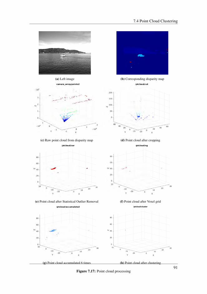
7.4 Point Cloud Clustering
(a) Left image (b) Corresponding disparity map
(c) Raw point cloud from disparity map (d) Point cloud after cropping
(e) Point cloud after Statistical Outlier Removal (f) Point cloud after Voxel grid
(g) Point cloud accumulated 6 times
/ptcloud/cluster
0
10
20
30
X
-20
-10
0
10
Y
0
20
40
60
80
Z
(h) Point cloud after clustering
Figure 7.17: Point cloud processing91

Chapter 7. Object detection
The implementation of the voxel grid filter is for real-time considerations. The voxelgrid downsamples the point cloud, approximating a neighborhood of points to the cen-troid. Using the filter enhances the computational time more than ten times! The lastpreprocessing function in line 13 accumulates the point clouds. It assembles subsequentpoint clouds for redundancy, increasing the reliability of the system. The function antic-ipates shortcomings in the stereo matching or filtering. If the stereo matching algorithmfails to match the objects of interest in one image, the accumulate function will includethe missing parts from the already processed point clouds. Also, objects of interest will bedenser, while noisier parts like sea waves remain sparse. The complete callback in Listing7.4 takes about ten milliseconds to compute accumulating 6 point clouds, by all meansdepending on the computer.
Both of the presented clustering techniques are used for object detection on milliAmpere.They are tested in the operational environment, and their performance is evaluated andcompared.
92

Chapter 8Test results in marine environment
The experiment and data collection took place outside the port of Brattøra. A handheldGlobal Positioning System (GPS), placed on the target boat, serves as the ground truth.The test area and the GPS route are shown in Figure 8.1. The origin of the NED coordinateframe is set inside the harbour. The performance of the stereo parameters obtained at 20
Figure 8.1: Test area and route of the target
meters, and the algorithms described in Chapter 7 are tested and evaluated.The experiment is divided into seven different scenarios, capturing the target boat at
different distances. The scenarios are numbered in chronological order by the time theywere recorded. The distance to the target varies between 10 and 160 meters. Scenariotwo, three, four, five and six are captured along the coast. The target is the main focus in
93

Chapter 8. Test results in marine environment
the scene, with the coast line and the island Munkholmen present in the background. Inscenario one and seven milliAmpere is following the target in and out of the harbour. Thisis to give an impression how the disparity map and the two clustering algorithms performin a confined environment. The parameters are not tuned for such an environment.
8.1 Ground truthA Garmin eTrex 10 GPS is placed right in front of the wheelhouse of the target boat,recording its positioning once per second. The GPS device has an accuracy of about 10meters (Luoto et al., 2010). Figure 8.2 shows the recorded GPS data during the experiment.
07:40:48 07:55:12 08:09:36 08:24:00 08:38:24 08:52:48 09:07:12
time- hours:minutes:seconds
63.4365
63.437
63.4375
63.438
63.4385
63.439
63.4395
63.44
63.4405
Lat
Lat Plot
21-May-2020
(a) GPS latitude
07:40:48 07:55:12 08:09:36 08:24:00 08:38:24 08:52:48 09:07:12
time- hours:minutes:seconds
10.388
10.39
10.392
10.394
10.396
10.398
10.4
Long
Long Plot
21-May-2020
(b) GPS longitude
07:40:48 07:55:12 08:09:36 08:24:00 08:38:24 08:52:48 09:07:12
time- hours:minutes:seconds
1
2
3
4
5
6
7
8
9
10
Ele
v
Elev Plot
21-May-2020
(c) GPS elevation
Figure 8.2: GPS plots
The test scenarios are all captured along the coast, thus no signal-blocking from buildingsis expected. During the data collection, there was little to no wind and a smooth sea. Theelevation plot in Figure 8.2c shows that the elevation varies between 1 and 10 meters.The varying elevation signal indicates that the GPS signal strength varies throughout theexperiment. In Figure G.2 in Appendix G the longitude, latitude and elevation plots aredivided into the different scenarios. Inspecting the plots, the GPS has smooth curves for
94
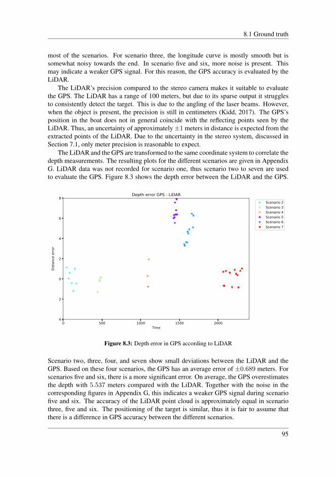
8.1 Ground truth
most of the scenarios. For scenario three, the longitude curve is mostly smooth but issomewhat noisy towards the end. In scenario five and six, more noise is present. Thismay indicate a weaker GPS signal. For this reason, the GPS accuracy is evaluated by theLiDAR.
The LiDAR’s precision compared to the stereo camera makes it suitable to evaluatethe GPS. The LiDAR has a range of 100 meters, but due to its sparse output it strugglesto consistently detect the target. This is due to the angling of the laser beams. However,when the object is present, the precision is still in centimeters (Kidd, 2017). The GPS’sposition in the boat does not in general coincide with the reflecting points seen by theLiDAR. Thus, an uncertainty of approximately±1 meters in distance is expected from theextracted points of the LiDAR. Due to the uncertainty in the stereo system, discussed inSection 7.1, only meter precision is reasonable to expect.
The LiDAR and the GPS are transformed to the same coordinate system to correlate thedepth measurements. The resulting plots for the different scenarios are given in AppendixG. LiDAR data was not recorded for scenario one, thus scenario two to seven are usedto evaluate the GPS. Figure 8.3 shows the depth error between the LiDAR and the GPS.
0 500 1000 1500 2000Time
−4
−2
0
2
4
6
8
Distan
ce erro
r
Depth error GPS - LiDARScenario 2Scenario 3Scenario 4Scenario 5Scenario 6Scenario 7
Figure 8.3: Depth error in GPS according to LiDAR
Scenario two, three, four, and seven show small deviations between the LiDAR and theGPS. Based on these four scenarios, the GPS has an average error of ±0.689 meters. Forscenarios five and six, there is a more significant error. On average, the GPS overestimatesthe depth with 5.537 meters compared with the LiDAR. Together with the noise in thecorresponding figures in Appendix G, this indicates a weaker GPS signal during scenariofive and six. The accuracy of the LiDAR point cloud is approximately equal in scenariothree, five and six. The positioning of the target is similar, thus it is fair to assume thatthere is a difference in GPS accuracy between the different scenarios.
95

Chapter 8. Test results in marine environment
The average error of scenario five is 6.551 meters while for six it is 4.625. Trustingthe LiDAR’s high accuracy, the mean error of scenario five and six is subtracted from theGPS. The resulting errors are illustrated in Figure 8.4. The GPS measures are assumed
0 500 1000 1500 2000Time
−4
−3
−2
−1
0
1
2
3
4
Distan
ce erro
r
Depth error GPS - LiDARstdScenario 2Scenario 3Scenario 4Scenario 5Scenario 6Scenario 7
Figure 8.4: Depth error in GPS adjusted according to LiDAR measurements
to include Gaussian distributed noise with mean e = 0.064, and a standard deviation ofσ = 0.865. The variance is therefore σ2 = 0.748. This seems reasonable as the LiDAR isexpected to have a standard deviation of around 1. Finally, it should be noted that the errorof the last point in scenario four deviates more than the other points in the same scenario.This may indicate that the GPS has a offset from the true position in the end of scenariofour.
Both the measurements by the GPS and the LiDAR are transformed into the NEDreference frame providing as the ground truth for evaluating the measurements of the stereocamera.
8.2 ResultsThis section presents the five test scenarios along the coast of Trondheim. The target iscaptured in a range of different distances to determine the stereo systems accuracy. Thetargets position is given in NED coordinates, and the distance to the target is calculatedrelative to milliAmpere. The resulting plots of the two clustering techniques; point cloud
96

8.2 Results
clustering and CNN clustering, are presented for each of the test scenarios. The estimateddistance to the target, the resulting error, and the NED position of the targets is given. Theposition in north and east direction depends on the time, and the plots of the directionsare given in Appendix H together with the corresponding errors. In each plot, the groundtruth is given in black, and the stereo systems estimates in blue. For all plots, distances aregiven in meters and time in seconds.
As already mentioned in Chapter 5, there may have been added a constant error tothe stereo setup. This will have a high influence on the overall results. However, thecomparison between the algorithms, and distance estimates is still valid. From Section7.1, the stereo system is expected to have a theoretical reprojection error of more than onepixel. For this reason, the theoretical reprojection error of one pixel is given in purpleand plotted together with the distance error of the stereo cameras. The expected distancebased on the theoretical error is included to illustrate what one pixel error corresponds toin distance for each scenario. The value of the reprojection error is given in Table 7.1, andplotted with the same sign as the error of the depth estimates.
8.2.1 Scenario 2
(a) Start of scenario 2 (b) End of scenario 2
Figure 8.5: Scenario 2
In the beginning of scenario 2, the stereo camera observes the aft of the target. In the mid-dle of the scenario the target makes a turn and places itself perpendicular to Milliamepre,see Figure 8.5. As the GPS is placed in front of the wheelhouse, a larger error is expectedin the first half of the scenario.
From the distance estimations in Figure 8.6, both clustering seems quite accurate. Thedistance is the optimal depth for the stereo system, and the result are therefore expectedto be the most satisfactory of all the scenes. However, Figure 8.8 show some deviationsfrom the theoretical error. As expected, the estimates are more accurate in the second halfof the scenario.
97

Chapter 8. Test results in marine environment
0 20 40 60 80 100 120 140 160Time
0
10
20
30
40
50
60
70
80Distance
CNN-clusteringground truthexpected stereo [1 pixel error]stereo
(a) Estimated distance
0 20 40 60 80 100 120 140 160Time
0
10
20
30
40
50
60
70
80
Distan
ce
ptCloud-clusteringground truthexpected stereo [1 pixel error]stereo
(b) Estimated distance
Figure 8.6: Distance estimate of scenario 2
−440 −430 −420 −410 −400 −390 −380 −370East
40
60
80
100
120
140
North
CNN-clustering
(a) Position in North-East
−440 −430 −420 −410 −400 −390 −380 −370East
40
60
80
100
120
140
North
ptCloud-clustering
(b) Position in North-East
Figure 8.7: Position estimate of scenario 2
0 20 40 60 80 100 120 140 160Time
−7
−6
−5
−4
−3
−2
−1
0
1
2
Distan
ce erro
r
CNN-clusteringexpected stereo [1 pixel error]error
(a) Error of estimated distance
0 20 40 60 80 100 120 140 160Time
−7
−6
−5
−4
−3
−2
−1
0
1
2
Distance
erro
r
ptCloud-clusteringexpected stereo [1 pixel error]error
(b) Error of estimated distance
Figure 8.8: Error of distance estimate of scenario 2
98
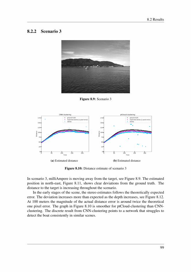
8.2 Results
8.2.2 Scenario 3
Figure 8.9: Scenario 3
0 50 100 150 200Time
0
25
50
75
100
125
150
175
Distan
ce
CNN-clusteringground truthexpected stereo [1 pixel error]stereo
(a) Estimated distance
0 50 100 150 200Time
0
25
50
75
100
125
150
175
Distan
ce
ptCloud-clusteringground truthexpected stereo [1 pixel error]stereo
(b) Estimated distance
Figure 8.10: Distance estimate of scenario 3
In scenario 3, milliAmpere is moving away from the target, see Figure 8.9. The estimatedposition in north-east, Figure 8.11, shows clear deviations from the ground truth. Thedistance to the target is increasing throughout the scenario.
In the early stages of the scene, the stereo estimates follows the theoretically expectederror. The deviation increases more than expected as the depth increases, see Figure 8.12.At 100 meters the magnitude of the actual distance error is around twice the theoreticalone pixel error. The graph in Figure 8.10 is smoother for ptCloud-clustering than CNN-clustering. The discrete result from CNN-clustering points to a network that struggles todetect the boat consistently in similar scenes.
99
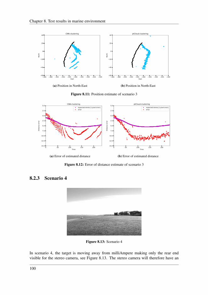
Chapter 8. Test results in marine environment
−465 −460 −455 −450 −445 −440 −435 −430 −425 −420East
−60
−40
−20
0
20
40No
rth
CNN-clustering
(a) Position in North-East
−465 −460 −455 −450 −445 −440 −435 −430 −425 −420East
−60
−40
−20
0
20
40
North
ptCloud-clustering
(b) Position in North-East
Figure 8.11: Position estimate of scenario 3
0 50 100 150 200Time
−15.0
−12.5
−10.0
−7.5
−5.0
−2.5
0.0
2.5
5.0
Distan
ce erro
r
CNN-clusteringexpected stereo [1 pixel error]error
(a) Error of estimated distance
0 50 100 150 200Time
−15.0
−12.5
−10.0
−7.5
−5.0
−2.5
0.0
2.5
5.0Distan
ce erro
rptCloud-clustering
expected stereo [1 pixel error]error
(b) Error of estimated distance
Figure 8.12: Error of distance estimate of scenario 3
8.2.3 Scenario 4
Figure 8.13: Scenario 4
In scenario 4, the target is moving away from milliAmpere making only the rear endvisible for the stereo camera, see Figure 8.13. The stereo camera will therefore have an
100

8.2 Results
0 20 40 60 80 100 120Time
0
20
40
60
80
100
120
140
160Distan
ce
CNN-clustering
ground truthexpected stereo [1 pixel error]stereo
(a) Estimated distance
0 20 40 60 80 100 120Time
0
20
40
60
80
100
120
140
160
Distan
ce
ptCloud-clustering
ground truthexpected stereo [1 pixel error]stereo
(b) Estimated distance
Figure 8.14: Distance estimate of scenario 4
offset from ground truth. The distance to the target is increasing but continues to a distanceof 150 meters.
Similar to scenario 3, for distances below 80 meters the estimates are within an ac-ceptable range, see Figure 8.14. At farther distances stronger deviations are present, andthe error exceeds 20 meters. During the last twenty second both algorithms fails to extractclusters, which implies the clusters from the disparity map are too small and considered asnoise for the algorithms. The estimates follows the shape of the curve, but with an increas-ing error. From Figure 8.15 CNN-clustering has a lower error, but point cloud clusteringhas a more consistent detection of the target throughout the scenario. The noise from thepoint cloud clustering originates from a noisy disparity map. In the last part of the scenethere is a significant large error. As mentioned in 8.1, the GPS might have an offset in themeasurement towards the end of scene 4.
−440 −420 −400 −380 −360 −340 −320 −300East
−150
−100
−50
0
50
100
North
CNN-clustering
(a) Position in North-East
−440 −420 −400 −380 −360 −340 −320 −300East
−150
−100
−50
0
50
100
North
ptCloud-clustering
(b) Position in North-East
Figure 8.15: Position estimate of scenario 4
For clarification, for a couple of seconds the target moves out of the stereo camerasfield of view. This occurs at position -50 North, -380 east in Figure 8.15, which correspondto time 40 (seconds).
101
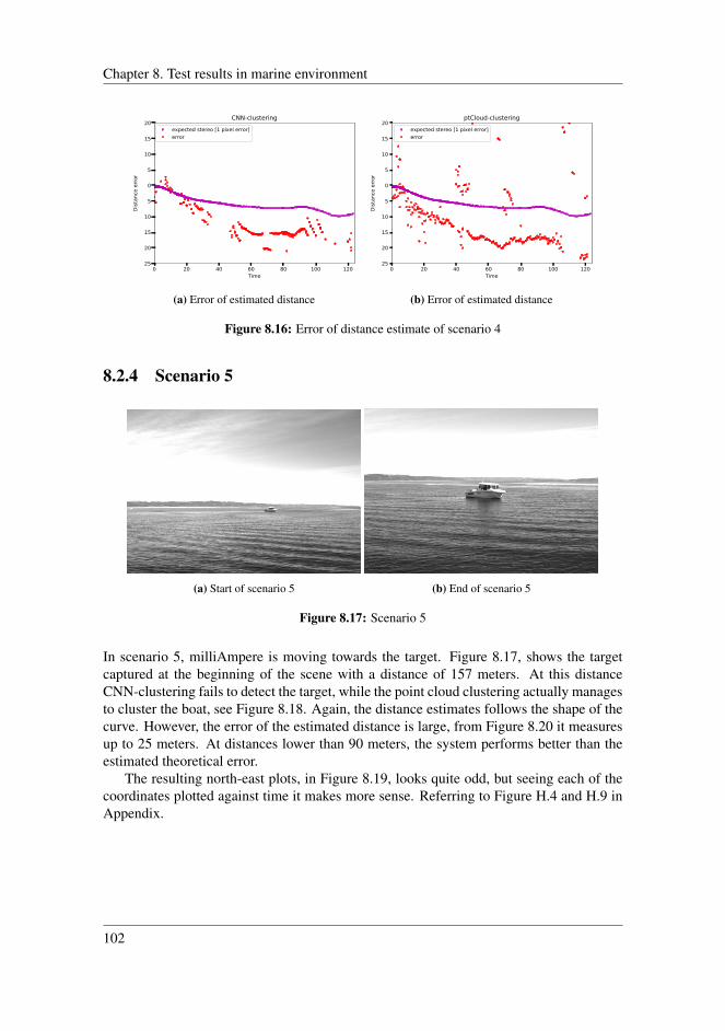
Chapter 8. Test results in marine environment
0 20 40 60 80 100 120Time
−25
−20
−15
−10
−5
0
5
10
15
20Distan
ce erro
r
CNN-clusteringexpected stereo [1 pixel error]error
(a) Error of estimated distance
0 20 40 60 80 100 120Time
−25
−20
−15
−10
−5
0
5
10
15
20
Distan
ce erro
r
ptCloud-clusteringexpected stereo [1 pixel error]error
(b) Error of estimated distance
Figure 8.16: Error of distance estimate of scenario 4
8.2.4 Scenario 5
(a) Start of scenario 5 (b) End of scenario 5
Figure 8.17: Scenario 5
In scenario 5, milliAmpere is moving towards the target. Figure 8.17, shows the targetcaptured at the beginning of the scene with a distance of 157 meters. At this distanceCNN-clustering fails to detect the target, while the point cloud clustering actually managesto cluster the boat, see Figure 8.18. Again, the distance estimates follows the shape of thecurve. However, the error of the estimated distance is large, from Figure 8.20 it measuresup to 25 meters. At distances lower than 90 meters, the system performs better than theestimated theoretical error.
The resulting north-east plots, in Figure 8.19, looks quite odd, but seeing each of thecoordinates plotted against time it makes more sense. Referring to Figure H.4 and H.9 inAppendix.
102

8.2 Results
0 20 40 60 80 100Time
0
20
40
60
80
100
120
140
160Distan
ce
CNN-clusteringground truthexpected stereo [1 pixel error]stereo
(a) Estimated distance
0 20 40 60 80 100Time
0
20
40
60
80
100
120
140
160
Distan
ce
ptCloud-clusteringground truthexpected stereo [1 pixel error]stereo
(b) Estimated distance
Figure 8.18: Distance estimate of scenario 5
−328 −326 −324 −322 −320 −318East
10
15
20
25
30
35
40
45
50
North
CNN-clustering
(a) Position in North-East
−328 −326 −324 −322 −320 −318East
10
15
20
25
30
35
40
45
50
North
ptCloud-clustering
(b) Position in North-East
Figure 8.19: Position estimate of scenario 5
0 20 40 60 80 100Time
−35
−30
−25
−20
−15
−10
−5
0
5
10
Distance
erro
r
CNN-clusteringexpected stereo [1 pixel error]error
(a) Error of estimated distance
0 20 40 60 80 100Time
−35
−30
−25
−20
−15
−10
−5
0
5
10
Distan
ce erro
r
ptCloud-clusteringexpected stereo [1 pixel error]error
(b) Error of estimated distance
Figure 8.20: Error of distance estimate of scenario 5
103
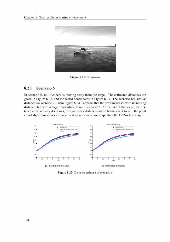
Chapter 8. Test results in marine environment
Figure 8.21: Scenario 6
8.2.5 Scenario 6In scenario 6, milliAmpere is moving away from the target. The estimated distances aregiven in Figure 8.22, and the world coordinates in Figure 8.23. The scenario has similardistances as scenario 2. From Figure 8.24 it appears that the error increases with increasingdistance, but with a larger magnitude than in scenario 2. At the end of the scene, the dis-tance error actually decreases, this yields for distances above 60 meters. Overall, the pointcloud algorithm serves a smooth and more dense error graph than the CNN-clustering.
0 10 20 30 40 50 60 70 80Time
0
10
20
30
40
50
60
70
80
90
Dist
ance
CNN-clusteringground truthexpected stereo [1 pixel error]stereo
(a) Estimated distance
0 10 20 30 40 50 60 70 80Time
0
10
20
30
40
50
60
70
80
90
Distance
ptCloud-clusteringground truthexpected stereo [1 pixel error]stereo
(b) Estimated distance
Figure 8.22: Distance estimate of scenario 6
104
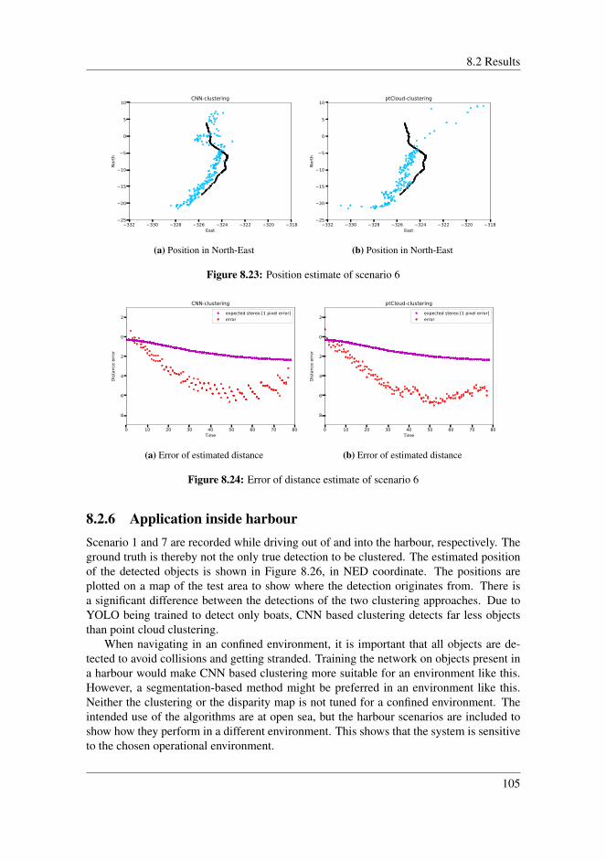
8.2 Results
−332 −330 −328 −326 −324 −322 −320 −318East
−25
−20
−15
−10
−5
0
5
10No
rth
CNN-clustering
(a) Position in North-East
−332 −330 −328 −326 −324 −322 −320 −318East
−25
−20
−15
−10
−5
0
5
10
North
ptCloud-clustering
(b) Position in North-East
Figure 8.23: Position estimate of scenario 6
0 10 20 30 40 50 60 70 80Time
−8
−6
−4
−2
0
2
Distan
ce erro
r
CNN-clusteringexpected stereo [1 pixel error]error
(a) Error of estimated distance
0 10 20 30 40 50 60 70 80Time
−8
−6
−4
−2
0
2Distance
erro
rptCloud-clustering
expected stereo [1 pixel error]error
(b) Error of estimated distance
Figure 8.24: Error of distance estimate of scenario 6
8.2.6 Application inside harbourScenario 1 and 7 are recorded while driving out of and into the harbour, respectively. Theground truth is thereby not the only true detection to be clustered. The estimated positionof the detected objects is shown in Figure 8.26, in NED coordinate. The positions areplotted on a map of the test area to show where the detection originates from. There isa significant difference between the detections of the two clustering approaches. Due toYOLO being trained to detect only boats, CNN based clustering detects far less objectsthan point cloud clustering.
When navigating in an confined environment, it is important that all objects are de-tected to avoid collisions and getting stranded. Training the network on objects present ina harbour would make CNN based clustering more suitable for an environment like this.However, a segmentation-based method might be preferred in an environment like this.Neither the clustering or the disparity map is not tuned for a confined environment. Theintended use of the algorithms are at open sea, but the harbour scenarios are included toshow how they perform in a different environment. This shows that the system is sensitiveto the chosen operational environment.
105

Chapter 8. Test results in marine environment
(a) Start of scenario 1 (b) End of scenario 1
(c) Start of scenario 7 (d) End of scenario 7
Figure 8.25: Recorded data from harbour
106

8.2 Results
(a) CNN-clustering scenario 1 (b) ptCloud clustering scenario 1
(c) CNN -clustering scenario 7 (d) ptCloud-clustering scenario 7
Figure 8.26: Estimated position of detected objects in harbour
107
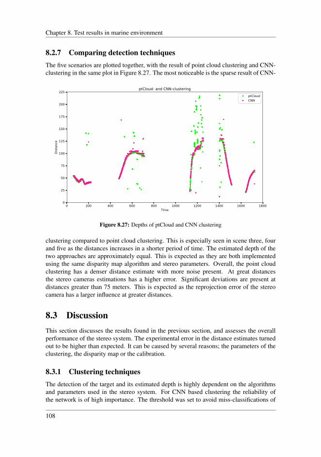
Chapter 8. Test results in marine environment
8.2.7 Comparing detection techniquesThe five scenarios are plotted together, with the result of point cloud clustering and CNN-clustering in the same plot in Figure 8.27. The most noticeable is the sparse result of CNN-
0 200 400 600 800 1000 1200 1400 1600 1800Time
0
25
50
75
100
125
150
175
200
225
Distan
ce
ptCloud- and CNN-clusteringptCloudCNN
Figure 8.27: Depths of ptCloud and CNN clustering
clustering compared to point cloud clustering. This is especially seen in scene three, fourand five as the distances increases in a shorter period of time. The estimated depth of thetwo approaches are approximately equal. This is expected as they are both implementedusing the same disparity map algorithm and stereo parameters. Overall, the point cloudclustering has a denser distance estimate with more noise present. At great distancesthe stereo cameras estimations has a higher error. Significant deviations are present atdistances greater than 75 meters. This is expected as the reprojection error of the stereocamera has a larger influence at greater distances.
8.3 DiscussionThis section discusses the results found in the previous section, and assesses the overallperformance of the stereo system. The experimental error in the distance estimates turnedout to be higher than expected. It can be caused by several reasons; the parameters of theclustering, the disparity map or the calibration.
8.3.1 Clustering techniquesThe detection of the target and its estimated depth is highly dependent on the algorithmsand parameters used in the stereo system. For CNN based clustering the reliability ofthe network is of high importance. The threshold was set to avoid miss-classifications of
108

8.3 Discussion
the same object in consecutive frames. The resulting plots shows few false positives, butincreased the number of false negatives. This caused a sparser output compared to pointcloud clustering. As a result of this, it seems like an even lower YOLO-threshold may befavourable.
Decreasing the precision further will results in more detections. However, with thegiven weights, the network tends to have FPs even for an YOLO-threshold approximatelyequal to 0. From the confusion matrix (7.8), a decrease in precision for the given weightsgives no noticeable increase in TP. This can also be seen from Figure 7.10 in Section7.3.2. The technique is limited to the quality of the network, and based on the results thenetworks performance can benefit from further training.
For the localization based on the YOLO-bounding boxes, the centroid and medianvalue gave a satisfying result. The distance estimates even seems to be more correct thanthe distances directly extracted from the point cloud. The inequalities in the depth es-timates between the two algorithms is most likely due to the network’s tendency to onlydetect parts of the boat. For the given test scenarios, the wrong positioning of the boundingboxes does not have any noticeable impact on the results. However, this should be notedas it may cause errors in different scenarios.
Point cloud clustering produces a dense output, but more false detections are present.This is a direct consequence of the chosen parameters. The wide range of distances inthe scenarios impose challenges for the selection of parameters. Setting a higher value forthe minimum number of points in a cluster would remove a lot of the noise. On the otherhand, for distances above 110 meters the target will be discarded as noise. Alternatively, anincrease in the number of accumulations or decreasing the value of the standard deviationmultiplier in the filtering, will discard some more noise. However, the noise is randomlydistributed and can thus be accounted for by standard Markovian models in a trackingalgorithm.
8.3.2 Disparity mapThe results are directly dependent on the parameter values of the disparity map. Thechosen parameter of the disparity map are optimal at approximately 50 meters, while thedistance to the target varies between 10 and 160 meters. Figure 8.28 shows examples ofthe resulting disparity maps at short, medium and far range distances. Figure 8.28b, 8.28eand 8.28g illustrated the original parameters set for point cloud clustering. At 140 metersnoise from the sea produces bigger clusters than the target. This causes the noise and lackof detection towards the end of scenario 4 in Figure 8.14. In the re-tuned disparity map inFigure 8.28h noise is removed by reducing the maximum disparity. This will segment outpoints at short distances. The minimum required points in a cluster can thus be decreased,making object detection optimal for far distances.
At 10 meters the resulting disparity map divides the boat into different segments. Thisis shown in Figure 8.26d, where both the target and the pier is segmented into severalparts, creating multiple detections of the same object. This also causes problems for CNNclustering, as it takes the median value of the disparities within a bounding box. When theobject appears sparse, the depth is estimated to infinity, e.g. no target is localized.
Considering the range of operating distances, it was hard to find optimal values. Fromthe results, the chosen disparity parameters performed better than expected considering
109
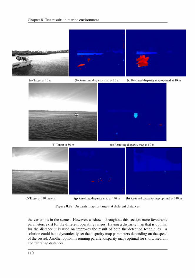
Chapter 8. Test results in marine environment
(a) Target at 10 m (b) Resulting disparity map at 10 m (c) Re-tuned disparity map optimal at 10 m
(d) Target at 50 m (e) Resulting disparity map at 50 m
(f) Target at 140 meters (g) Resulting disparity map at 140 m (h) Re-tuned disparity map optimal at 140 m
Figure 8.28: Disparity map for targets at different distances
the variations in the scenes. However, as shown throughout this section more favourableparameters exist for the different operating ranges. Having a disparity map that is optimalfor the distance it is used on improves the result of both the detection techniques. Asolution could be to dynamically set the disparity map parameters depending on the speedof the vessel. Another option, is running parallel disparity maps optimal for short, mediumand far range distances.
110

8.3 Discussion
8.3.3 Error of the estimated distances
The mean percentage error of the two clustering techniques is plotted in Figure 8.29. Theerror is calculated from the ground truth. The CNN-clustering yields an average absoluteerror percentage of 0.069, and the point cloud clustering 0.076. These calculations arebased on a adjusted ground truth, combining the GPS measurements with the LiDAR. Inaddition, 2 meters are removed from scenario 4 and the beginning of scenario 2 to accountfor the GPS’s position in the boat. From the Figure 8.29, the magnitude of the error varies
0 100 200 300 400 500 600 700Time
−0.2
−0.1
0.0
0.1
0.2
Distance
erro
r [%]
CNN-clusteringScenario 2Scenario 3Scenario 4Scenario 5Scenario 6
(a) Percentage error of estimated distance from CNN-clustering
0 100 200 300 400 500 600 700Time
−0.2
−0.1
0.0
0.1
0.2
Distance erro
r [%]
ptClo d-clusteringScenario 2Scenario 3Scenario 4Scenario 5Scenario 6
(b) Percentage error of estimated distance from ptCloud-clustering
Figure 8.29: Percentage error of estimated distance from the ground truth for all scenarios
between the scenarios. The percentage error is three times as high as the error from thetest scenes in Chapter 5.
It is worth noticing that there seems to be a constant offset, a bias. This is probably dueto errors in the estimation of the focal length or the baseline. Both directly influences thedepth estimates (2.10). A constant error can also have occurred due to the transformationbetween the camera and the GPS on milliAmpere being measured by hand.
111

Chapter 8. Test results in marine environment
8.3.4 Reprojection error
0 100 200 300 400 500 600 700Time
−25
−20
−15
−10
−5
0
5
10
Distan
ce erro
r
CNN-clustering
Expected stereo [1 pixel error]Scenario 2Scenario 3Scenario 4Scenario 5Scenario 6
(a) CNN-clustering
0 100 200 300 400 500 600 700Time
−25
−20
−15
−10
−5
0
5
10
Distan
ce erro
r
ptCloud-clustering
Expected stereo [1 pixel error]Scenario 2Scenario 3Scenario 4Scenario 5Scenario 6
(b) ptCloud-clustering
Figure 8.30: Error of all scenario and expected value when there is a pixel error of 1
In Figure 8.30, the error of all scenarios are given with the expected value when onepixel error is present. This confirms that the theoretical reprojection error is too optimistic.To find the true reprojection error for the system, equation (8.1) is minimized.
µ(e(dist)) =1
N
∑(diststereo − (distGT + e(dist))) (8.1)
diststereo is the estimated distance from the stereo camera, distGT is the ground truth dis-tance, and e(dist) is the reprojection error given in pixels. This gave the CNN-clusteringa reprojection error of 1.588 pixels, and the point cloud clustering 1.988 pixels. One mayargue that the expected value should be zero, however this confirms that there is a constantoffset in the stereo system.
Figure 8.31a and 8.31b shows how the estimated distance from the stereo camera devi-ates from the given reprojection error. Point cloud clustering yields a higher reprojection
112
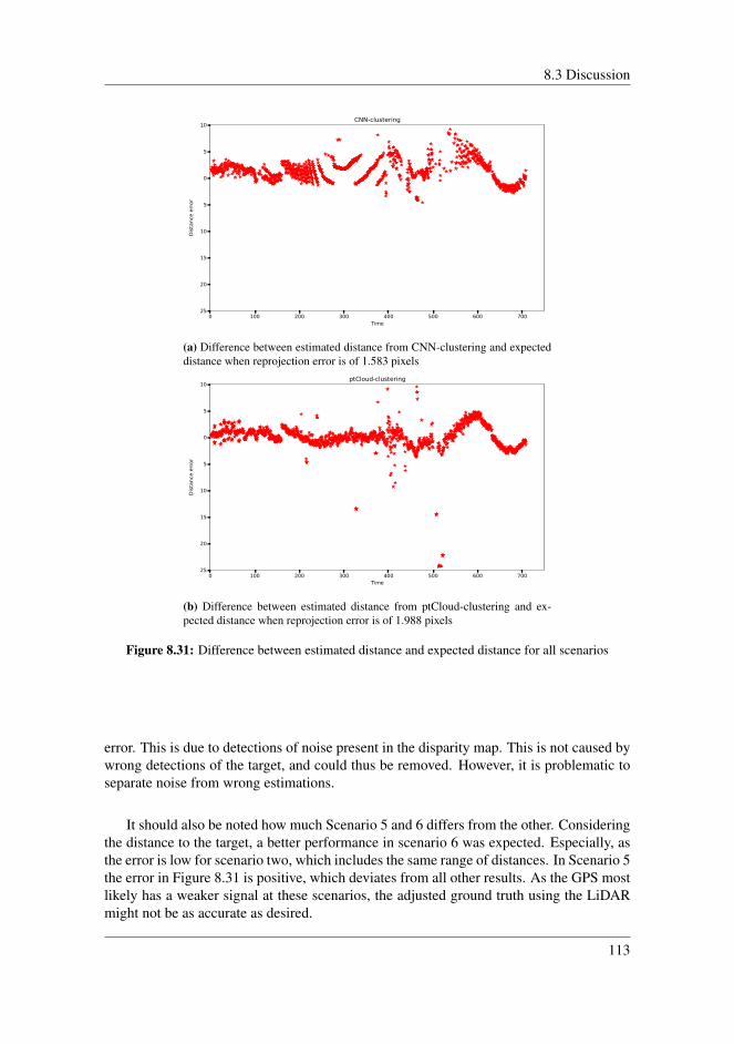
8.3 Discussion
0 100 200 300 400 500 600 700Time
−25
−20
−15
−10
−5
0
5
10
Distan
ce erro
r
CNN-clustering
(a) Difference between estimated distance from CNN-clustering and expecteddistance when reprojection error is of 1.583 pixels
0 100 200 300 400 500 600 700Time
−25
−20
−15
−10
−5
0
5
10
Distan
ce erro
r
ptCloud-clustering
(b) Difference between estimated distance from ptCloud-clustering and ex-pected distance when reprojection error is of 1.988 pixels
Figure 8.31: Difference between estimated distance and expected distance for all scenarios
error. This is due to detections of noise present in the disparity map. This is not caused bywrong detections of the target, and could thus be removed. However, it is problematic toseparate noise from wrong estimations.
It should also be noted how much Scenario 5 and 6 differs from the other. Consideringthe distance to the target, a better performance in scenario 6 was expected. Especially, asthe error is low for scenario two, which includes the same range of distances. In Scenario 5the error in Figure 8.31 is positive, which deviates from all other results. As the GPS mostlikely has a weaker signal at these scenarios, the adjusted ground truth using the LiDARmight not be as accurate as desired.
113
Chapter 8. Test results in marine environment
8.3.5 Uncertainty in the stereo systemThe standard deviation of the Figures 8.31a and 8.31b, measures the expected uncertaintiesof the system. With a mean of 1.583 pixels, the standard deviation of CNN-clustering iscalculated to 3.882 meters. For the ptCloud-clustering the standard deviation is 6.921meters calculated from a mean value of 1.988 pixels.
The standard deviation of ptCloud-clustering is of significant size. By removing sce-nario 5 and 6, the standard deviation is reduced to 2.668 meters. The distribution of pointsmay indicate a Gaussian distribution. Assuming this, ptCloud-clustering has a variance of1.633 meters. Removing scenario 5 and 6 impose no significant changes to the measuredstandard deviation of CNN-clustering. The depth error, shown in Table 8.1, indicates the
Real world-depth Disparity Depth error
CNN-clusteringDepth error
ptCloud-clustering10 m 229.3 ±0.070m ±0.087 m20 m 114.7 ±0.277m -±.348 m30 m 76.5 ±0.621m ±0.779 m40 m 57.3 ±1.107m ±1.390 m50 m 45.9 ±1.727m ±2.169 m60 m 38.2 ±2.488m ±3.125 m70 m 32.8 ±3.384m ±4.250 m80 m 28.7 ±4.423m ±5.554 m90 m 25.5 ±5.605m ±7.040 m
100 m 22.9 ±6.922m ±8.694 m110 m 20.9 ±8.350m ±10.487 m120 m 19.1 ±9.952m ±12.499 m130 m 17.7 ±11.654m ±14.636 m140 m 16.4 ±13.498m ±16.952 m150 m 15.3 ±15.509m ±19.476 m
Table 8.1: Expected depth error for CNN-clustering (1.583 pixels) and ptCloud-clustering (1.988)
expected reprojection error under the assumption that the disparity error is 1.583 and 1.988pixel.
8.3.6 Limitations of the stereo systemThe experimental measured error and standard deviation turned out to be higher than inthe theoretical consideration where more optimistic estimations about the possible setupand measurement deviations was made. It can be caused by several reasons which finallyaccumulate to a higher error. This includes higher errors in the estimation of the baselineand the relative orientation of the cameras but also higher errors in the estimation of thematching position of corresponding points.
There is a constant offset in the distance estimates. The constant offset indicates errorsin the estimates of the stereo parameters. This will influence both the reconstruction ofworld points and the rectification which directly affects the stereo matching.
114

8.3 Discussion
The results indicates range limitations. In general, the disparity map of objects atfar distances produces a sparse cluster of points. Figure 8.28h shows that even for anoptimal disparity map at 140 meters, the target appears in relatively few pixels. At 140meters an object will have a displacement of 16.4 pixels. Due to uncertainties in the stereomatching, the stereo system is likely to have range limit of approximately 200 meters. Thiscorresponds to a displacement of only 11 pixels. To have an operational system at suchgreat distances, a tuning of the disparity map and the point cloud clustering algorithm isimperative. With the stereo systems calculated reprojection error an object at 200 metersyields a depth error of almost 50 meters. Therefore, the baseline must be widened toreduce the slope of the depth error, based on the reprojection error and baseline (Figure7.1b).
8.3.7 Overall performanceSome error in the estimated distance to the target is tolerable when the uncertainty of thesystem is known. From the ground truth, the reprojection error was calculated to 1.583and 1.988 pixels for CNN-clustering and ptCloud-clustering, respectively. With additionaltesting, the uncertainty of the system can be determined more accurately.
Two operational clustering algorithms has been implemented, as well as a stereo match-ing procedure. The range of distances imposes challenges for setting optimal parametersfor all scenarios. The result of point cloud clustering is influenced by noise present in thedisparity map. While, for CNN-clustering the result is dependent on the quality of thenetwork. Even though miss-classifications and lack of detections occurred, the target wasdetected and localized for all scenarios. The CNN based clustering procedure is robustagainst noise in the disparity map. Point cloud clustering is more prone to noise in thedisparity map, but gave a more dense and consistent result.
Scenario 1 and 7 show how sensitive the behavior of the system is to changes in theenvironment. For the system to produce beneficial results in these scenarios, an adjust-ment of the parameters is necessary. The performance of the system is dependent on setparameters and the operational environment. Using different parameters of the algorithmsat different distances, could also help improve the overall result. However, the utilizedparameters provided a reasonable result considering the wide range of distances in thescenarios. Overall, the parameters extracts the target and estimates the distance with aoffset. With further testing of the system using a more reliable ground truth a lower uncer-tainty is expected.
115

Chapter 8. Test results in marine environment
116

Chapter 9Conclusion and future work
9.1 Conclusion
A stereo setup for an autonomous ferry was introduced, calibrated, implemented andtested. A far range extrinsic calibration procedure was proposed, and tested on scenesof different depths. The LiDAR was used as the ground truth to confirm that extrinsiccalibration highly influence the accuracy of the reconstructed world points. The findingsshowed that a careful selection of the scene is of higher importance than calibrating at theoperating distance. A scene where salient points are available in the cameras entire fieldof view will improve the calibration accuracy.
A ROS-based software architecture for object detection was implemented and tested ina marine environment. The disparity map was implemented using a correlation basedcorrespondence algorithm, and Fast Global Image Smoothing Based on Weighted LeastSquares. This provided a robust foundation for clustering. Two different techniques wereutilized for object detection. A convolution neural network was applied for classification,and used in combination with the disparity map to extract 3D positions of objects. Themethod is robust against noise in the disparity map, but appeared to be partially incon-sistent in the estimates. However, the technique is limited to the quality of the network.The alternative detection method based on hierarchical clustering using Euclidean distancemade consistent detections, but was more prone to noise in the disparity map. The noisecan be accounted for by standard Markovian models in a tracking algorithm.
The system was tested on the autonomous ferry milliAmpere, and the targets was detectedand its localization given in the common world frame. With a stereo configuration optimalfor 50 meters, the stereo system was found to have a reprojection error of 1.583 and 1.988pixels, for CNN- and ptCloud-clustering respectively. The average absolute error for thesystems distance estimates is 7%. With additional testing, the uncertainty of the systemcan be determined more accurately. Based on the constant bias, the error is expected to beadjusted to a more acceptable range. While the implemented system shows potential, it is
117

Chapter 9. Conclusion and future work
still not clear that the detection performance is good enough to rely on these methods inan autonomous collision avoidance system.
9.2 Future WorkThe thesis has experimented with a stereo configuration for use on an autonomous ferry.The work has laid the foundation for using stereo camera for visual vessel detection onan unmanned surface vehicles in general. The system was tested in the operation envi-ronment, in and close to Trondheim Harbor, but there are still several issues to be solvedbefore the proposed stereo vision solution can be used as a part of a sensor fusion system.Therefore, the following tasks are suggested to continue the work of this thesis.
• Due to COVID-19 and bad weather conditions opportunities for testing was limited.More tests of the system needs to be performed to find a more exact estimate of theuncertainty. In the test scenarios presented, the ground truth originates from a GPScorrected by LiDAR data. A more reliable ground truth would be provided by e.g, aGPS using RTK.
• The stereo camera system should be properly mounted and integrated on milliAmpere.This allows for a calibration for finding the rigid-body transformation between thestereo camera and the BODY frame of the vessel. This will improve the accuracyof the system. When a proper calibration of the stereo camera and milliAmpere’sBODY frame is performed, the resulting 3D coordinate frames should be imple-mented using the ROS-library tf. This will make the information about the coordi-nate frames available to all ROS components.
• The physical constraints of the cameras needs to be taken into consideration. Theoperating temperature is above 0 degrees and they are not waterproof. The stereosetup is also sensitive to changes in temperature, vibrations and wind, causing theaccuracy of the extrinsic stereo calibration to fluctuate over time.
• As already mentioned, more favourable disparity maps parameters exists for the dif-ferent operating distances. Looking into dynamically set disparity maps dependingon the speed, or running multiple maps in parallel could improve the result of boththe detection techniques.
• The real-time capabilities of the system must be assessed. The running time of thesystem is imperative for the reliability and usefulness of the output data. YOLO isrunning on the GPU, using CUDA to reduce the running time. The CUDA toolkitcan be useful throughout the system, especially for the point cloud clustering andstereo matching. For the overall system all the image processing will benefit of beingin the same package. Implementing the nodes as nodelets will minimize memoryusage, running multiple algorithms in the same process with zero-copy transportbetween algorithms.
• Comparing different extrinsic stereo parameters in a marine environment would ofinterest. The stereo camera parameters are set in the Spinnaker driver. As the sce-
118
9.2 Future Work
narios were recorded using bagfiles, a dynamic change of the parameters on thecaptured data was not performed.
• Because of the constant bias, both the internal and external parameters of the stereocamera should be re-calibrated. When performing the stereo calibration the datashould be normalized when performing linear triangulation. This will improve thenumerical estimates in DLT. When evaluating the parameters the main focus wason depth. A further evaluation of the influencing factors of, and the accuracy ofreconstructed x- and y-coordinates should be performed.
• The accuracy of the stereo camera is dependent on the estimations of the extrin-sic parameters, thus changes in the configurations can lead wrongly reconstructed3D points. Marita et al. (2006) proposed an on-line calibration method for moni-toring the stability of the relative extrinsic parameters. The method is suitable foroutdoor far range stereo 3D reconstruction applications. Accounting for externalfactors influencing the physical system would also be beneficial for the stereo cam-era mounted on milliAmpere.
• Widening the baseline and imposing a global method for stereo matching would in-crease the accuracy of the system. If a global method is used, then running time mustbe taken into consideration. Generally, global methods require more computationalpower than local methods.
• The possibility of fusing the stereo camera with other sensors should be examined.If data from different sensors are combined it will be possible to achieve less uncer-tainty than for a pure stereo camera system.
119

Chapter 9. Conclusion and future work
120
Bibliography
Abdullah, Sukarnur Che, e.a., 2019. Stereo vision for visual object tracking and distancemeasurement assessment. Journal of Mechanical Engineering 16, 121–134.
Benjdira, B., Khursheed, T., Koubaa, A., Ammar, A., Ouni, K., 2019. Car detection usingunmanned aerial vehicles: Comparison between faster R-CNN and YOLOv3, in: 20191st International Conference on Unmanned Vehicle Systems-Oman (UVS), pp. 1–6.
Biber, P., Straßer, W., 2003. The normal distributions transform: A new approach to laserscan matching, in: Proceedings 2003 IEEE/RSJ International Conference on IntelligentRobots and Systems (IROS 2003), pp. 2743–2748.
Christensen, H.I., Bowyer, K., Bunke, H., 1993. Active Robot Vision: camera heads,model based navigation and reactive control. volume 6. World Scientific.
Curtin, D.P., 2011. Understanding the Baseline. URL: http://www.shortcourses.com/stereo/stereo3-14.html.
Fooladgar, F., Samavi, S., Soroushmehr, S.M.R., Shirani, S., 2013. Geometrical analysisof localization error in stereo vision systems. IEEE Sensors Journal 13, 4236 – 4246.
Fossen, T.I., 2011. Handbook of marine craft hydrodynamics and motion control. JohnWiley & Sons.
G., C., Stephens, M., 1988. A combined corner and edge detector. Alvey vision conference15, 10–5244.
Golub, G.H., Van Loan, C.F., 2013. Matrix computations. volume 4th. JHU press.
Grini, S.V., 2019. Object Detection in Maritime Environments. Master’s thesis. NTNU.
Hartley, R., Zisserman, A., 2004. Multiple View Geometry in computer vision, 2nd edi-tion. Cambridge University Press.
Hirschmuller, H., 2005. Accurate and efficient stereo processing by semi-global matchingand mutual information, in: 2005 IEEE Computer Society Conference on ComputerVision and Pattern Recognition (CVPR’05), pp. 807–814 vol. 2.
121
Hirschmuller, H., 2011. Semi-global matching-motivation, developments and applica-tions. Photogrammetric Week 11 , 173–184.
Hirschmuller, H., Gehrig, S., 2009. Stereo matching in the presence of sub-pixel calibra-tion errors, in: 2009 IEEE Conference on Computer Vision and Pattern Recognition,IEEE. pp. 437–444.
Huber, P.J., 1985. Projection pursuit. The annals of Statistics , 435–475.
Kidd, J.R., 2017. Performance evaluation of the Velodyne VLP-16 system for surfacefeature surveying .
Konolige, K., 1998. Small vision systems: Hardware and implementation, in: Roboticsresearch. Springer, pp. 203–212.
Krenker, A., Bester, J., Kos, A., 2011. Introduction to the artificial neural networks, in:Suzuki, K. (Ed.), Artificial Neural Networks. IntechOpen, Rijeka. chapter 1.
Kukelova, Z., Martin, B., Pajdla, T., 2008. Polynomial eigenvalue solutions to the 5-PTand 6-PT relative pose problems. BMVC 2, 138–156.
Li, L., Zhang, S., Wu, J., 2019. Efficient object detection framework and hardware archi-tecture for remote sensing images. Remote Sensing 11, 2376.
Li, Y., Min, D., Do, M.N., Lu, J., 2016. Fast guided global interpolation for depth andmotion. European Conference on Computer Vision , 717–733.
Liu, Y., Aggarwal, J., 2005. Local and Global Stereo Methods. chapter 3.12. pp. 297–308.
Luoto, M., Marmion, M., Hjort, J., 2010. Assessing spatial uncertainty in predictive geo-morphological mapping: A multi-modelling approach. Computers & Geosciences 36,355–361.
Magnusson, M., 2009. The Three-Dimensional Normal-Distributions Transform — anEfficient Representation for Registration, Surface Analysis, and Loop Detection. Ph.D.thesis. Orebro University, School of Science and Technology.
Marita, T., Oniga, F., Nedevschi, S., Graf, T., Schmidt, R., 2006. Camera calibrationmethod for far range stereovision sensors used in vehicles. IEEE Intelligent VehiclesSymposium , 356 – 363.
McCabe, K., 2016. How to Set Up a Stereo Machine Vision So-lution. URL: https://www.qualitymag.com/articles/93543-how-to-set-up-a-stereo-machine-vision-solution.
Min, D., Choi, S., Lu, J., Ham, B., Sohn, K., Do, M.N., 2014. Fast global image smoothingbased on weighted least squares. IEEE Transactions on Image Processing 23, 5638–5653.
Nguyen, A., Le, B., 2013. 3d point cloud segmentation: A survey, in: 2013 6th IEEEconference on robotics, automation and mechatronics (RAM), IEEE. pp. 225–230.
122
Nguyen, P.H., Ahn, C.W., 2019. Stereo matching methods for imperfectly rectified stereoimages. Symmetry 11, 570.
Ødegard Olsen, T., 2020. Stereo vision using local methods for autonomous ferry. 5thyear specialization project at NTNU.
O’Shea, K., Nash, R., 2015. An introduction to convolutional neural net-works. CoRR abs/1511.08458. URL: http://arxiv.org/abs/1511.08458,arXiv:1511.08458.
Park, K., Kim, S., Sohn, K., 2018. High-precision depth estimation with the 3d lidar andstereo fusion, in: 2018 IEEE International Conference on Robotics and Automation(ICRA), pp. 2156–2163.
Pendleton, S., Andersen, H., Du, X., Shen, X., Meghjani, M., Eng, Y., Rus, D., Ang,M., 2017. Perception, Planning, Control, and Coordination for Autonomous Ve-hicles. Machines 5, 6. URL: http://www.mdpi.com/2075-1702/5/1/6,doi:10.3390/machines5010006.
Praveen, S., 2019. Efficient depth estimation using sparse stereo-vision with other percep-tion techniques, in: Advanced Image and Video Coding. IntechOpen.
Quigley, M., Conley, K., Gerkey, B.P., Faust, J., Foote, T., Leibs, J., Wheeler, R.C., Ng,A.Y., 2009. ROS: an open-source robot operating system, in: IEEE International Con-ference on Robotics and Automation.
Redmon, J., Divvala, S.K., Girshick, R.B., Farhadi, A., 2015. You only look once: Uni-fied, real-time object detection. CoRR abs/1506.02640. URL: http://arxiv.org/abs/1506.02640, arXiv:1506.02640.
Redmon, J., Farhadi, A., 2018. YOLOv3: An incremental improvement.CoRR abs/1804.02767. URL: http://arxiv.org/abs/1804.02767,arXiv:1804.02767.
robotics, O., . Spinnaker SDK driver - ROS wiki . http://wiki.ros.org/spinnaker_sdk_camera_driver. Open Source Robotics Foundation.
Rusu, R.B., Cousins, S., 2011. 3D is here: Point Cloud Library (PCL), in: IEEE Interna-tional Conference on Robotics and Automation (ICRA), Shanghai, China. pp. 1–4.
Sasiadek, J.Z., Walker, M.J., 2019. Achievable stereo vision depth accuracy with changingcamera baseline. 24th International Conference on Methods and Models in Automationand Robotics (MMAR), Miedzyzdroje, Poland , 152–157.
Schiller, I., Beder, C., Koch, R., 2012. Calibration of a PMD-camera using a planarcalibration pattern together with a multi-camera setup. ISPRS 37.
Shi, J., Tomasi, C., 1994. Good features to track. IEEE conference on computer visionand pattern recognition 2, 593–600.
123

Shin, B., Mou, X., Mou, W., 2018. Vision-based navigation of an unmanned surfacevehicle with object detection and tracking abilities. Machine Vision and Applications29, 95–112.
Strecha, C., Von Hansen, W., Van Gool, L., Fua, P., Thoennessen, U., 2008. On bench-marking camera calibration and multi-view stereo for high resolution imagery. IEEEConference on Computer Vision and Pattern Recognition , 1 – 8.
Templeton, B., 2013. Cameras or Lasers? URL: https://www.templetons.com/brad/robocars/cameras-lasers.html.
Thaher, R.H., Hussein, Z.K., 2014. Stereo vision distance estimation employing SAD withCanny edge detector. International Journal of Computer Applications 107.
Theimann, L., 2020. Comparison of depth information from stereo camera and lidar. 5thyear specialization project at NTNU.
Tomasi, C., Kanade, T., 1991. Detection and tracking of point features. InternationalJournal of Computer Vision .
Torr, P.H.S., Zisserman, A., 2000. MLESAC: A new robust estimator with application toestimating image geometry. Computer Vision and Image Understanding 78, 138–156.
Velodyne, 2019. Velodyne LiDAR Puck. Technical report.
Wang, Y., Chao, W.L., Garg, D., Hariharan, B., Campbell, M., Weinberger, K.Q., 2019.Pseudo-lidar from visual depth estimation: Bridging the gap in 3D object detection forautonomous driving. Proceedings of the IEEE Conference on Computer Vision andPattern Recognition URL: http://arxiv.org/abs/1812.07179.
Wang, Y., Lai, Z., Huang, G., Wang, B.H., van der Maaten, L., Campbell, M., Wein-berger, K.Q., 2019. Anytime stereo image depth estimation on mobile devices, in: 2019International Conference on Robotics and Automation (ICRA), pp. 5893–5900.
Wang, Y., Wang, X., Yin, L., 2019. Estimation of extrinsic parameters for dynamic binoc-ular stereo vision using unknown-sized rectangle images. Review of Scientific Instru-ments 90, 065108.
Warren, M., McKinnon, D., , Upcroft, B., 2013. Online calibration of stereo rigs forlong-term autonomy. IEEE International Conference on Robotics and Automation 37,3692–3698.
Yu, S., Zhu, R., Yu, L., Ai, W., 2018. Effect of checkerboard on the accuracy of cameracalibration. Pacific Rim Conference on Multimedia , 619–629.
Zhang, Z., 2000. A flexible new technique for camera calibration. IEEE Transactions onpattern analysis and machine intelligence 22, 1330 – 1334.
Zhao, Z.Q., Zheng, P., Xu, S.T., Wu, X., 2019. Object detection with deep learning: Areview. IEEE transactions on neural networks and learning systems 30, 3212–3232.
124

Appendix AReconstructed point clouds ofcalibration scenes
This appendix contains plots of the reconstructed point clouds of each calibration scene.The obtained stereo parameters are used in a semi-global matching algorithm to create adisparity map and to reconstruct a point cloud of the calibration scene. The point cloudsare plotted together with the ground truth of the scene, the LiDAR point cloud. The stereopoint cloud is given in green and the LiDAR in purple.
125

(a) 10 meters front (b) 10 meters above (c) 20 meters front (d) 20 meters above
(e) 30 meters front (f) 30 meters above (g) 40 meters front (h) 40 meters above
(i) 40 meters front (j) 40 meters above (k) 50 meters front (l) 50 meters above
(m) 60 meters front (n) 60 meters above (o) 70 meters front (p) 70 meters above
Figure A.1: Stereo point cloud of calibration scenes plotted together with LiDAR point cloud
126

Appendix BReconstructed point clouds of testscenes
This appendix contains plots of the stereo point clouds of each test scene. The point cloudsare plotted together with the ground truth of the scene, the LiDAR point cloud. The stereopoint cloud is given in green and the LiDAR in purple.
(a) 7.6 meter MATLAB calibration (b) 10 meter calibration (c) 20 meter calibration
(d) 30 meter calibration (e) 40 meter calibration (f) 50 meter calibration
127

(g) 60 meter calibration (h) 70 meter calibration (i) Average calibration
Figure B.1: Test scene at 30 meters
(a) 7.6 meter MATLAB calibration (b) 10 meter calibration (c) 20 meter calibration
(d) 30 meter calibration (e) 40 meter calibration (f) 50 meter calibration
(g) 60 meter calibration (h) 70 meter calibration (i) Average calibration
Figure B.2: Test scene at 40 meters
128

(a) 7.6 meter MATLAB calibration (b) 10 meter calibration (c) 20 meter calibration
(d) 30 meter calibration (e) 40 meter calibration (f) 50 meter calibration
(g) 60 meter calibration (h) 70 meter calibration (i) Average calibration
Figure B.3: Test scene at 50 meters
129

(a) 7.6 meter MATLAB calibration (b) 10 meter calibration (c) 20 meter calibration
(d) 30 meter calibration (e) 40 meter calibration (f) 50 meter calibration
(g) 60 meter calibration (h) 70 meter calibration (i) Average calibration
Figure B.4: Test scene at 70 meters
130
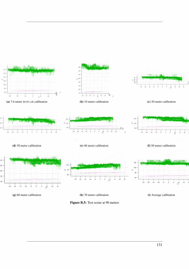
(a) 7.6 meter MATLAB calibration (b) 10 meter calibration (c) 20 meter calibration
(d) 30 meter calibration (e) 40 meter calibration (f) 50 meter calibration
(g) 60 meter calibration (h) 70 meter calibration (i) Average calibration
Figure B.5: Test scene at 90 meters
131

132
Appendix CGithub repository, Readme
133

README.md
Stereo Vision for Autonomous ferry - code
The project is a part of TTK4900 - Engineering Cybernetics, Master's Thesis at Norwegian University of Science and Technology. "Stereo
Vision for Autonomous ferry" goes into detail of the calibration, the chosen stereo setup, and the implementation for testing of dynamic
scenes. The ownship has adequate data to sense, process, and understand its surroundings.
Contents
Getting Started
System overviw
Launch
Connect to Network MilliAmpere
Application and Scrips
Authors and License
Getting Started
Example of the stereo system tested. The baseline in use measures 1.8meters, and the cameras are angled 1 degree inwards. The stereo
system was tested using Blackfly S GigE with PoE, master software triggering, and GPIO pins for external triggering of the slave. The
Velodyne LiDAR Puck-16 serves as ground truth for the system.
Prerequisites
Set up a computer with GPU and Ubuntu 16.04. The repo is tested on a Dell Precision 7530 with NVIDIA Quadro P3200.
Set up a stereo system, and perform a stereo calibration of the cameras.
Install Spinnaker and verify that you can run your cameras with SpinViw (Windows operating system is preferred). Set up a stereo
system with either hardware or software triggering. Modify the yaml files in spinnaker-sdk-driver by replacing the cam-ids and master
cam serial number to match your camera's serial number. In the same yaml file, include the calibration parameters. (If using Matlab
for calibration, make sure to convert the numbers to OpenCV calibration definitions)
Optionally: Set up the LiDAR driver. An extrinsic calibration of the LiDAR and the stereo camera must be performed for the LiDAR to
serve as a basis for comparison.
Installing
README.md - Grip http://localhost:6419/
1 of 5 6/16/20, 11:33 PM
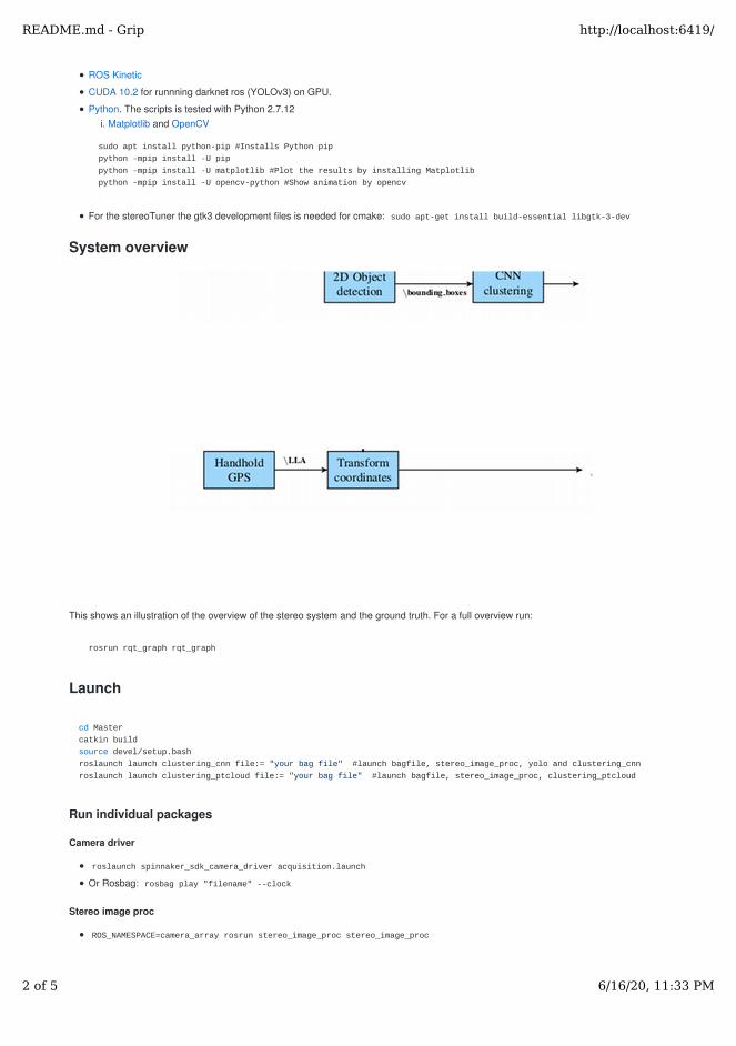
ROS Kinetic
CUDA 10.2 for runnning darknet ros (YOLOv3) on GPU.
Python. The scripts is tested with Python 2.7.12
i. Matplotlib and OpenCV
sudo apt install python-pip #Installs Python pip
python -mpip install -U pip
python -mpip install -U matplotlib #Plot the results by installing Matplotlib
python -mpip install -U opencv-python #Show animation by opencv
For the stereoTuner the gtk3 development files is needed for cmake: sudo apt-get install build-essential libgtk-3-dev
System overview
This shows an illustration of the overview of the stereo system and the ground truth. For a full overview run:
rosrun rqt_graph rqt_graph
Launch
cd Master
catkin build
source devel/setup.bash
roslaunch launch clustering_cnn file:= "your bag file" #launch bagfile, stereo_image_proc, yolo and clustering_cnn
roslaunch launch clustering_ptcloud file:= "your bag file" #launch bagfile, stereo_image_proc, clustering_ptcloud
Run individual packages
Camera driver
roslaunch spinnaker_sdk_camera_driver acquisition.launch
Or Rosbag: rosbag play "filename" --clock
Stereo image proc
ROS_NAMESPACE=camera_array rosrun stereo_image_proc stereo_image_proc
README.md - Grip http://localhost:6419/
2 of 5 6/16/20, 11:33 PM

Display images
Rectified images and disparity map`
i. rosrun image_view stereo_view stereo:=/camera_array image:=image_rect_color
Raw stereo images 2. rosrun image_view stereo_view stereo:=/camera_array image:=image_raw
Left rectified image 3. rosrun image_view image_view image:=/camera_arr/left/image_rect_color
Clustering Point Cloud
roslaunch clustering pcl_obstacle_detector.launch #Need the bagfile to be run with the "--clock"
Tuning the parameters: rosrun rqt_reconfigure rqt_reconfigure
Visualize in rviz: rosrun rviz rviz -f velodyne The package filters and clusters the point cloud, publishing the point clouds, and
transforms the clusters to NED coordinates. The class makes use of PassThrough filter, Statistical Outlier Removal, Voxel Grid filter,
accumulates subsequent point clouds, and Euclidean clustering.
Darknet_ros (YOLOv3)
roslaunch darknet_ros yolo_v3.launch #subscribes on camera_array/left/image_rect_color
Clustering Convolutional Neural Network
rosrun clustering_cnn clustering_cnn
Navigation data
rosrun navigation_data *filename*
Connect to Network on MilliAmpere
If the code is to be run with the master core on the ferry Milliampere a local network needs to be setup. The best solution is to set up a
separate static network on the computer through usb3.
ifconfig #find your network
sudo nano /etc/network/interfaces #add/make the network static
nano /etc/hosts #add milliAmpere as host on machine, further do the same at milliAmpere
sudo ifdown "your network" && sudo ifup "your network" #restarting interface
ping milliAmpere #check if connection established
Now that you have created a static network, the roscore has to be exported. This tells your machine that the roscore is running on another
computer. Be sure to do this in every terminal window (can be an advantage to add in nano .bashrc)
export ROS_MASTER_URI=http://milliAmpere:11311
echo $ROS_MASTER_URI
rostopic echo /topic #test that connection is established
Application and Scripts
stereoTuner
Application for tuning the disparity map, implemented using the stereoBM object and WLS filter from openCV. The GUI is a modified
version of the repository stereo-tuner. Remember to rectify the images beforehand; you're welcome. It is a simple little GTK application
that can be used to tune parameters for the OpenCV Stereo Vision algorithms.
mkdir build
cd build
cmake ..
make
./main
README.md - Grip http://localhost:6419/
3 of 5 6/16/20, 11:33 PM

Label YOLO images
GUI for marking bounded boxes of objects in images for training Yolo v3.
Put your .jpg -images in the directory x64/Release/data/img .
Change the numer of classes (objects for detection) in file `x64/Release/data/obj.data
Put names of the objects, one for each line in the file `x64/Release/data/obj.names If the images are used for training a custom
dataset visit AlexBA for a more detailed explanation.
cmake .
make
./linux_mark.sh
Precision-recall curve for YOLOv3
Plots and calculates the precision-recall curve from ground truth images. It iterates through two for-loops, one with IoU-threshold and the
second with the YOLO-threshold. Make sure to input detection images from the network with threshold less than the ones in the for-loop in
main.py. The mAP script is a modified version of the code in the github repository mAp. It outputs a precision-recall curve for each
threshold and IoU-threshold in main.py
Create the ground truth files using Label YOLO images
i. Insert images into the folder input/ground-truth/images
README.md - Grip http://localhost:6419/
4 of 5 6/16/20, 11:33 PM

ii. Insert ground-truth files into ground-truth/
iii. Add class list to the file scripts/extra/class_list.txt
iv. Run the python script: python convert_gt_yolo.py to convert the txt-files to the correct format
Create the detection-results files by running darknet_ros (It is created code (commented out) for saving box-files and rectified images
in /src/darknet_ros/darknet_ros/src/YoloObjectDetector.cpp)
i. Copy the detection-results files into the folder input/detection-results/
Run the script: python main.py
i. Note: To run the script once, for a given IoU-threshold and YOLO-threshold,run the following command line. This wil process
mAP, detection result information etc in the folder /output. python precision-recall.py "IoU-threshold" "YOLO-threshold"
Note: be consistent with using rectified/not-rectified images.
python main.py
Feel free to edit the main file with your preferred values in the for-loops.
Plot and calculate ground truth depth and stereo depth
Matches handhold-GPS csv file with the GPS from MA by satellite time. Match the stereo ros-time and plots estimated depth and NED
coordinates in a beautiful graph.
Authors and License
Good-luck from two soon-to-be well educated grown-ups.
Trine Ødegård Olsen - trineoo
Lina Theimann - linact
This project is licensed under the MIT License - see the LICENSE.md file for details
README.md - Grip http://localhost:6419/
5 of 5 6/16/20, 11:33 PM

Appendix DLabeling ground truth dataset forYOLOv3 evaluation
To evaluate the accuracy of the weights in the network, a ground truth dataset was labeled.The dataset is captured outside the port Brattøra and consists of 483 images. The imagesare rectified with the given calibration parameters, and manually labeled with the graphicaluser interface developed by AlexeyAB1. The GUI created for marking bounded boxes ofobjects in images for neural network is shown in Figure D.2. The GUI output a textfilefor each image, containing the class of labeled objects with the corresponding boundingbox. The dataset contains images of one boat at different heading from the camera’s pointof view. All the images are taken 40- to 150-meters from the boat. An example of thepictures in the dataset is displayed in Figure D.1. The pictures are easy to label and areconsidered a relatively fair scene considering the training set. The dataset is expected toyield satisfactory results, given the operating environment.
1https://github.com/AlexeyAB/Yolo_mark
139

Figure D.1: Images of the dataset
Figure D.2: GUI for labeling images
140

Appendix EResult of differentYOLO-thresholds
With IoU-threshold of 0.2, different YOLO-threshold yields the following result. Used tofind the systems optimal threshold.
YOLO-threshold
IoU >= 0.20Area Precision Recall
0.03 0.2379 0.2379 1.00000.04 0.2379 0.2379 1.00000.05 0.2379 0.2379 1.00000.06 0.2564 0.2564 1.00000.07 0.2712 0.2712 1.00000.08 0.2880 0.2880 1.00000.09 0.3028 0.3028 1.00000.10 0.3205 0.3205 1.00000.11 0.3371 0.3371 1.00000.12 0.3526 0.3526 1.00000.13 0.3698 0.3698 1.00000.14 0.3861 0.3861 1.00000.15 0.4022 0.4022 1.00000.16 0.4178 0.4178 1.00000.17 0.4347 0.4347 1.00000.18 0.4476 0.4476 1.00000.19 0.4649 0.4649 1.00000.20 0.4792 0.4792 1.00000.21 0.4898 0.4908 0.9979
......
......
141

YOLO-threshold
IoU >= 0.20Area Precision Recall
0.22 0.5037 0.5047 0.99790.23 0.5172 0.5183 0.99790.24 0.5368 0.5379 0.99790.25 0.5503 0.5515 0.99790.26 0.5659 0.5671 0.99790.27 0.5747 0.5783 0.99380.28 0.5847 0.5909 0.98960.29 0.5940 0.6015 0.98760.30 0.6025 0.6140 0.98140.31 0.6087 0.6216 0.97930.32 0.6232 0.6391 0.97520.33 0.6318 0.6479 0.97520.34 0.6378 0.6582 0.96890.35 0.6450 0.6686 0.96480.36 0.6508 0.6789 0.95860.37 0.6519 0.6830 0.95450.38 0.6579 0.6923 0.95030.39 0.6603 0.6994 0.94410.40 0.6594 0.7093 0.92960.41 0.6664 0.7217 0.92340.42 0.6633 0.7265 0.91300.43 0.6610 0.7356 0.89860.44 0.6665 0.7470 0.89230.45 0.6631 0.7590 0.87370.46 0.6540 0.7648 0.85510.47 0.6478 0.7669 0.84470.48 0.6390 0.7697 0.83020.49 0.6379 0.7780 0.81990.50 0.6356 0.7851 0.80950.51 0.6394 0.7939 0.80540.52 0.6434 0.8071 0.79710.53 0.6402 0.8137 0.78670.54 0.6277 0.8172 0.76810.55 0.6266 0.8247 0.75980.56 0.6171 0.8326 0.74120.57 0.6097 0.8413 0.72460.58 0.6079 0.8536 0.71220.59 0.6064 0.8589 0.70600.60 0.5877 0.8575 0.68530.61 0.5852 0.8670 0.67490.62 0.5639 0.8674 0.6501
......
......
142
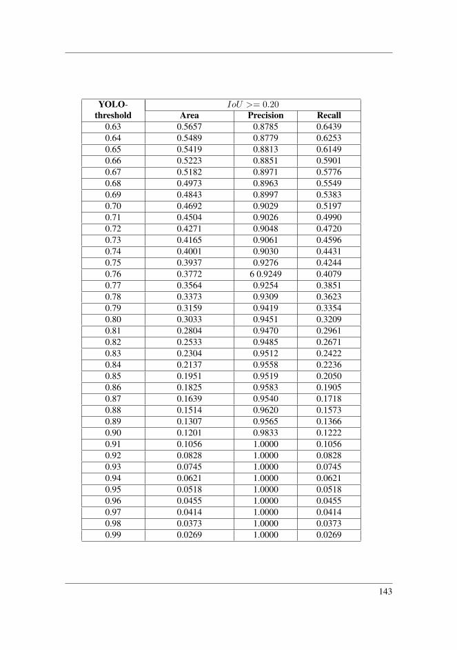
YOLO-threshold
IoU >= 0.20Area Precision Recall
0.63 0.5657 0.8785 0.64390.64 0.5489 0.8779 0.62530.65 0.5419 0.8813 0.61490.66 0.5223 0.8851 0.59010.67 0.5182 0.8971 0.57760.68 0.4973 0.8963 0.55490.69 0.4843 0.8997 0.53830.70 0.4692 0.9029 0.51970.71 0.4504 0.9026 0.49900.72 0.4271 0.9048 0.47200.73 0.4165 0.9061 0.45960.74 0.4001 0.9030 0.44310.75 0.3937 0.9276 0.42440.76 0.3772 6 0.9249 0.40790.77 0.3564 0.9254 0.38510.78 0.3373 0.9309 0.36230.79 0.3159 0.9419 0.33540.80 0.3033 0.9451 0.32090.81 0.2804 0.9470 0.29610.82 0.2533 0.9485 0.26710.83 0.2304 0.9512 0.24220.84 0.2137 0.9558 0.22360.85 0.1951 0.9519 0.20500.86 0.1825 0.9583 0.19050.87 0.1639 0.9540 0.17180.88 0.1514 0.9620 0.15730.89 0.1307 0.9565 0.13660.90 0.1201 0.9833 0.12220.91 0.1056 1.0000 0.10560.92 0.0828 1.0000 0.08280.93 0.0745 1.0000 0.07450.94 0.0621 1.0000 0.06210.95 0.0518 1.0000 0.05180.96 0.0455 1.0000 0.04550.97 0.0414 1.0000 0.04140.98 0.0373 1.0000 0.03730.99 0.0269 1.0000 0.0269
143

144

Appendix FThe milliAmpere system
The system running on Milliampere can be comprised in the following graph.
145
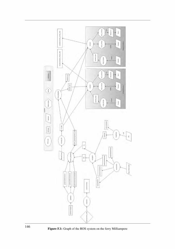
Figure F.1: Graph of the ROS system on the ferry Milliampere146
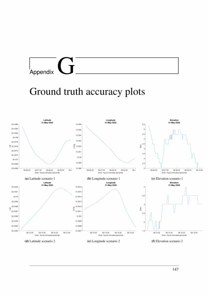
Appendix GGround truth accuracy plots
08:06:00 08:07:00 08:08:00 08:09:00 08:10:00
time- hours:minutes:seconds
63.4366
63.4368
63.437
63.4372
63.4374
63.4376
63.4378
63.438
63.4382
63.4384
63.4386
Lat
Latitude
21-May-2020
(a) Latitude scenario 1
08:06:00 08:07:00 08:08:00 08:09:00 08:10:00
time- hours:minutes:seconds
10.388
10.389
10.39
10.391
10.392
10.393
10.394
10.395
10.396
Long
Longitude
21-May-2020
(b) Longitude scenario 1
08:06:00 08:07:00 08:08:00 08:09:00 08:10:00
time- hours:minutes:seconds
2
2.5
3
3.5
4
4.5
5
5.5
6
6.5
Ele
v
Elevation
21-May-2020
(c) Elevation scenario 1
08:13:30 08:14:00 08:14:30 08:15:00
time- hours:minutes:seconds
63.4393
63.4394
63.4395
63.4396
63.4397
63.4398
63.4399
63.44
63.4401
63.4402
Lat
Latitude
21-May-2020
(d) Latitude scenario 2
08:13:30 08:14:00 08:14:30 08:15:00
time- hours:minutes:seconds
10.3907
10.3908
10.3909
10.391
10.3911
10.3912
10.3913
10.3914
10.3915
10.3916
Long
Longitude
21-May-2020
(e) Longitude scenario 2
08:13:30 08:14:00 08:14:30 08:15:00
time- hours:minutes:seconds
1.5
2
2.5
3
3.5
4
Ele
v
Elevation
21-May-2020
(f) Elevation scenario 2
147

08:20:00 08:21:00 08:22:00 08:23:00 08:24:00
time- hours:minutes:seconds
63.4385
63.4386
63.4387
63.4388
63.4389
63.439
63.4391
63.4392
Lat
Latitude
21-May-2020
(a) Latitude scenario 3
08:20:00 08:21:00 08:22:00 08:23:00 08:24:00
time- hours:minutes:seconds
10.39008
10.3901
10.39012
10.39014
10.39016
10.39018
10.3902
10.39022
10.39024
10.39026
10.39028
Long
Longitude
21-May-2020
(b) Longitude scenario 3
08:20:00 08:21:00 08:22:00 08:23:00 08:24:00
time- hours:minutes:seconds
5.8
6
6.2
6.4
6.6
6.8
7
7.2
7.4
Ele
v
Elevation
21-May-2020
(c) Elevation scenario 3
08:31:00 08:31:30 08:32:00 08:32:30 08:33:00
time- hours:minutes:seconds
63.4375
63.438
63.4385
63.439
63.4395
63.44
Lat
Latitude
21-May-2020
(d) Latitude scenario 4
08:31:00 08:31:30 08:32:00 08:32:30 08:33:00
time- hours:minutes:seconds
10.39
10.3905
10.391
10.3915
10.392
10.3925
Long
Longitude
21-May-2020
(e) Longitude scenario 4
08:31:00 08:31:30 08:32:00 08:32:30 08:33:00
time- hours:minutes:seconds
3.5
4
4.5
5
5.5
6
6.5
7
7.5
8
Ele
v
Elevation
21-May-2020
(f) Elevation scenario 4
08:35:30 08:36:00 08:36:30 08:37:00 08:37:30
time- hours:minutes:seconds
63.43915
63.4392
63.43925
63.4393
63.43935
63.4394
Lat
Latitude
21-May-2020
(g) Latitude scenario 5
08:35:30 08:36:00 08:36:30 08:37:00 08:37:30
time- hours:minutes:seconds
10.39259
10.3926
10.39261
10.39262
10.39263
10.39264
10.39265
10.39266
10.39267
10.39268
10.39269
Long
Longitude
21-May-2020
(h) Longitude scenario 5
08:35:30 08:36:00 08:36:30 08:37:00 08:37:30
time- hours:minutes:seconds
2.5
3
3.5
4
4.5
Ele
v
Elevation
21-May-2020
(i) Elevation scenario 5
148
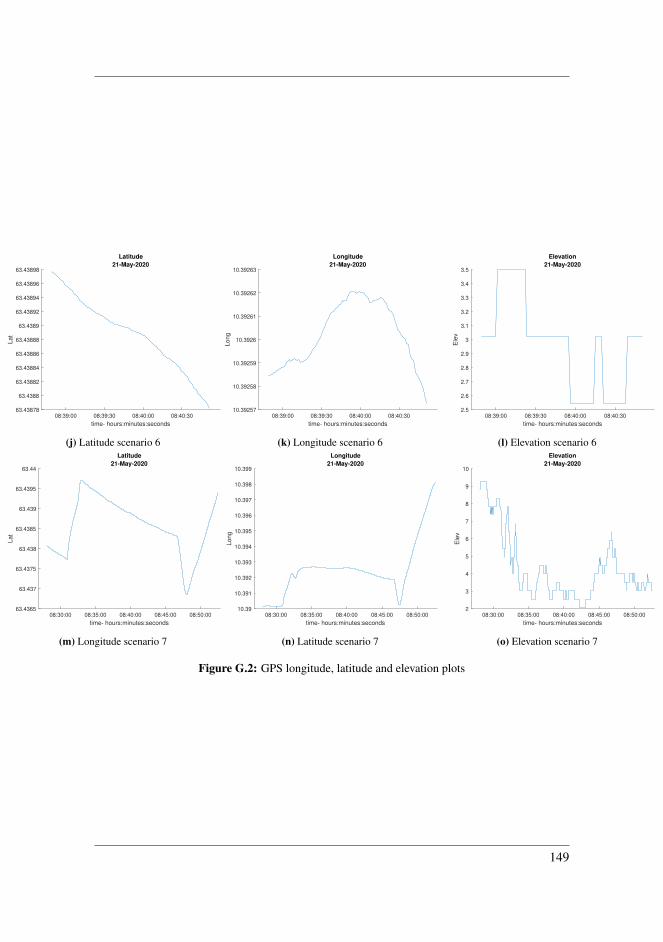
08:39:00 08:39:30 08:40:00 08:40:30
time- hours:minutes:seconds
63.43878
63.4388
63.43882
63.43884
63.43886
63.43888
63.4389
63.43892
63.43894
63.43896
63.43898
Lat
Latitude
21-May-2020
(j) Latitude scenario 6
08:39:00 08:39:30 08:40:00 08:40:30
time- hours:minutes:seconds
10.39257
10.39258
10.39259
10.3926
10.39261
10.39262
10.39263
Long
Longitude
21-May-2020
(k) Longitude scenario 6
08:39:00 08:39:30 08:40:00 08:40:30
time- hours:minutes:seconds
2.5
2.6
2.7
2.8
2.9
3
3.1
3.2
3.3
3.4
3.5
Ele
v
Elevation
21-May-2020
(l) Elevation scenario 6
08:30:00 08:35:00 08:40:00 08:45:00 08:50:00
time- hours:minutes:seconds
63.4365
63.437
63.4375
63.438
63.4385
63.439
63.4395
63.44
Lat
Latitude
21-May-2020
(m) Longitude scenario 7
08:30:00 08:35:00 08:40:00 08:45:00 08:50:00
time- hours:minutes:seconds
10.39
10.391
10.392
10.393
10.394
10.395
10.396
10.397
10.398
10.399
Long
Longitude
21-May-2020
(n) Latitude scenario 7
08:30:00 08:35:00 08:40:00 08:45:00 08:50:00
time- hours:minutes:seconds
2
3
4
5
6
7
8
9
10
Ele
vElevation
21-May-2020
(o) Elevation scenario 7
Figure G.2: GPS longitude, latitude and elevation plots
149

0 20 40 60 80 100 120 140 160Time
0
20
40
60
80
100
120
140
Depth
Scenario 2depth from
GPSLiDAR
(a) Scene 2
0 50 100 150 200Time
0
20
40
60
80
100
120
140
Depth
Scenario 3depth from
GPSLiDAR
(b) Scene 3
0 20 40 60 80 100 120Time
0
20
40
60
80
100
120
140
Depth
Scenario 4depth from
GPSLiDAR
(c) Scene 4
0 20 40 60 80 100Time
0
20
40
60
80
100
120
140
Depth
Scenario 5depth from
GPSLiDAR
(d) Scene 5
0 20 40 60 80 100 120Time
0
20
40
60
80
100
120
140
Depth
Scenario 6depth from
GPSLiDAR
(e) Scene 6
0 50 100 150 200 250 300 350Time
0
20
40
60
80
100
120
140
Depth
Scenario 7depth from
GPSLiDAR
(f) Scene 7
Figure G.3: Depth from LiDAR and GPS
150

Appendix HResult Plots
H.1 CNN-clustering
151

0 20 40 60 80 100 120 140 160Time
40
60
80
100
120
140
160
North
Scenario 2
(a) North-time
0 20 40 60 80 100 120 140 160Time
−460
−450
−440
−430
−420
−410
−400
−390
−380
−370
East
Scenario 2
(b) East-time
0 20 40 60 80 100 120 140 160Time
−40
−30
−20
−10
0
10
20
30
North
erro
r
Scenario 2
(c) North-time error
0 20 40 60 80 100 120 140 160Time
−10.0
−7.5
−5.0
−2.5
0.0
2.5
5.0
7.5
10.0Ea
st erro
rScenario 2
(d) East-time error
0 20 40 60 80 100 120 140 160Time
−0.25
−0.20
−0.15
−0.10
−0.05
0.00
0.05
Depth error [%]
Scenario 2
(e) Depth-time error percentage
Figure H.1: Scenario 2
152

0 50 100 150 200Time
−40
−30
−20
−10
0
10
20
North
Scenario 3
(a) North-time
0 50 100 150 200Time
−455
−450
−445
−440
−435
East
Scenario 3
(b) East-time
0 50 100 150 200Time
−40
−30
−20
−10
0
10
20
30
North
erro
r
Scenario 3
(c) North-time error
0 50 100 150 200Time
−10.0
−7.5
−5.0
−2.5
0.0
2.5
5.0
7.5
10.0
East erro
rScenario 3
(d) East-time error
0 50 100 150 200Time
−0.25
−0.20
−0.15
−0.10
−0.05
0.00
0.05
Depth error [%]
Scenario 3
(e) Depth-time error percentage
Figure H.2: Scenario 3
153

0 20 40 60 80 100 120Time
−100
−50
0
50
North
Scenario 4
(a) North-time
0 20 40 60 80 100 120Time
−440
−420
−400
−380
−360
−340
East
Scenario 4
(b) East-time
0 20 40 60 80 100 120Time
−40
−30
−20
−10
0
10
20
30
North
erro
r
Scenario 4
(c) North-time error
0 20 40 60 80 100 120Time
−10.0
−7.5
−5.0
−2.5
0.0
2.5
5.0
7.5
10.0Ea
st erro
rScenario 4
(d) East-time error
0 20 40 60 80 100 120Time
−0.25
−0.20
−0.15
−0.10
−0.05
0.00
0.05
Depth error [%]
Scenario 4
(e) Depth-time error percentage
Figure H.3: Scenario 4
154

0 20 40 60 80 100Time
−20
0
20
40
60
80
North
Scenario 5
(a) North-time
0 20 40 60 80 100Time
−350
−340
−330
−320
−310
−300
East
Scenario 5
(b) East-time
0 20 40 60 80 100Time
−40
−30
−20
−10
0
10
20
30
North
erro
r
Scenario 5
(c) North-time error
0 20 40 60 80 100Time
−10.0
−7.5
−5.0
−2.5
0.0
2.5
5.0
7.5
10.0Ea
st erro
rScenario 5
(d) East-time error
0 20 40 60 80 100Time
−0.25
−0.20
−0.15
−0.10
−0.05
0.00
0.05
Depth error [%]
Scenario 5
(e) Depth-time error percentage
Figure H.4: Scenario 5
155

0 10 20 30 40 50 60 70 80Time
−40
−30
−20
−10
0
10
North
Scenario 6
(a) North-time
0 10 20 30 40 50 60 70 80Time
−350
−340
−330
−320
−310
−300
East
Scenario 6
(b) East-time
0 10 20 30 40 50 60 70 80Time
−40
−30
−20
−10
0
10
20
30
North
erro
r
Scenario 6
(c) North-time error
0 10 20 30 40 50 60 70 80Time
−10.0
−7.5
−5.0
−2.5
0.0
2.5
5.0
7.5
10.0Ea
st erro
rScenario 6
(d) East-time error
0 10 20 30 40 50 60 70 80Time
−0.25
−0.20
−0.15
−0.10
−0.05
0.00
0.05
Depth error [%]
Scenario 6
(e) Depth-time error percentage
Figure H.5: Scenario 6
156
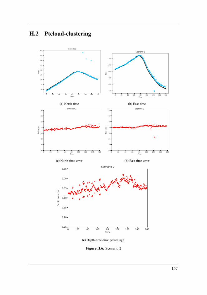
H.2 Ptcloud-clustering
0 20 40 60 80 100 120 140 160Time
50
75
100
125
150
175
200
225
250
North
Scenario 2
(a) North-time
0 20 40 60 80 100 120 140 160Time
−430
−420
−410
−400
−390
−380
East
Scenario 2
(b) East-time
0 20 40 60 80 100 120 140 160Time
−40
−30
−20
−10
0
10
20
30
North
erro
r
Scenario 2
(c) North-time error
0 20 40 60 80 100 120 140 160Time
−40
−30
−20
−10
0
10
20
30
East erro
r
Scenario 2
(d) East-time error
0 20 40 60 80 100 120 140 160Time
−0.25
−0.20
−0.15
−0.10
−0.05
0.00
0.05
Depth error [%]
Scenario 2
(e) Depth-time error percentage
Figure H.6: Scenario 2
157
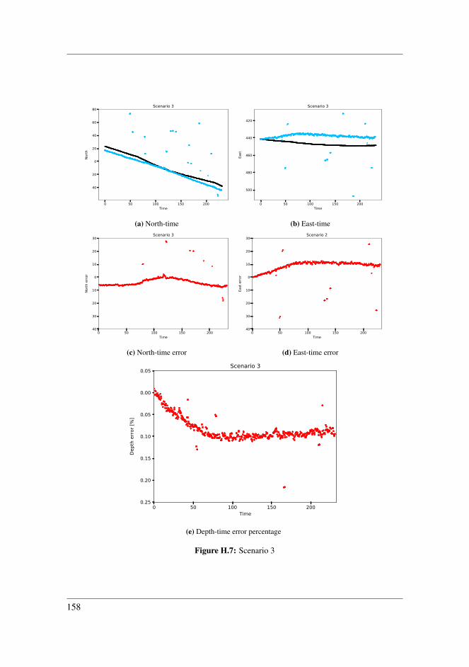
0 50 100 150 200Time
−40
−20
0
20
40
60
80
North
Scenario 3
(a) North-time
0 50 100 150 200Time
−500
−480
−460
−440
−420
East
Scenario 3
(b) East-time
0 50 100 150 200Time
−40
−30
−20
−10
0
10
20
30
North
erro
r
Scenario 3
(c) North-time error
0 50 100 150 200Time
−40
−30
−20
−10
0
10
20
30Ea
st erro
rScenario 2
(d) East-time error
0 50 100 150 200Time
−0.25
−0.20
−0.15
−0.10
−0.05
0.00
0.05
Depth error [%]
Scenario 3
(e) Depth-time error percentage
Figure H.7: Scenario 3
158
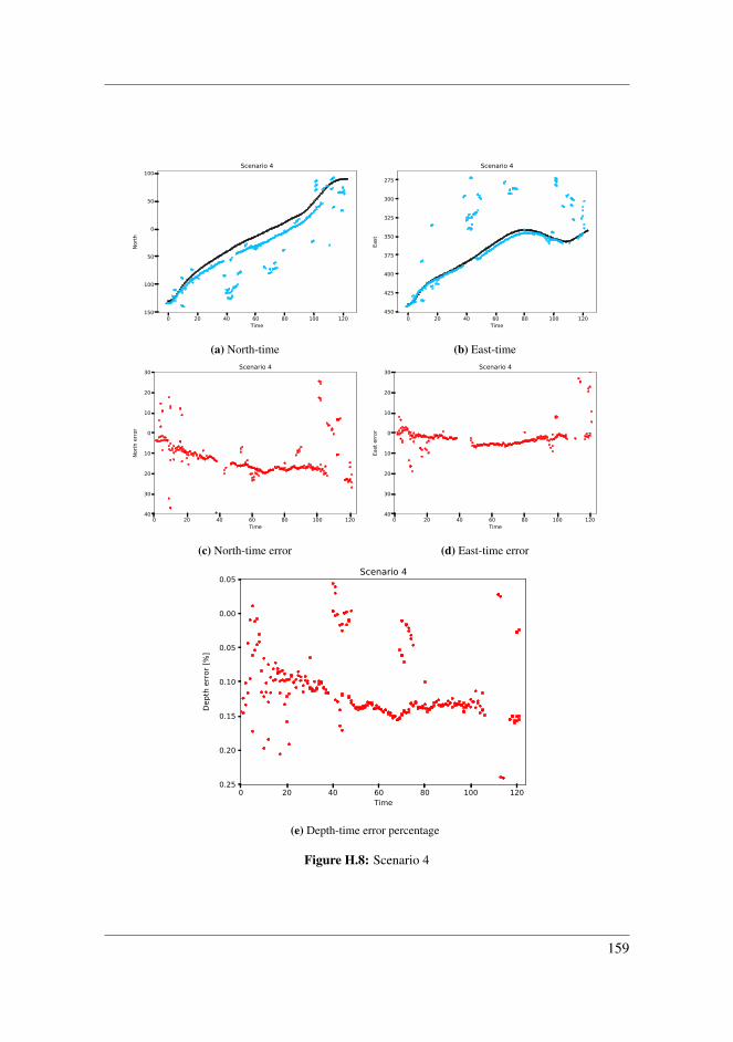
0 20 40 60 80 100 120Time
−150
−100
−50
0
50
100
North
Scenario 4
(a) North-time
0 20 40 60 80 100 120Time
−450
−425
−400
−375
−350
−325
−300
−275
East
Scenario 4
(b) East-time
0 20 40 60 80 100 120Time
−40
−30
−20
−10
0
10
20
30
North
erro
r
Scenario 4
(c) North-time error
0 20 40 60 80 100 120Time
−40
−30
−20
−10
0
10
20
30Ea
st erro
rScenario 4
(d) East-time error
0 20 40 60 80 100 120Time
−0.25
−0.20
−0.15
−0.10
−0.05
0.00
0.05
Depth error [%]
Scenario 4
(e) Depth-time error percentage
Figure H.8: Scenario 4
159
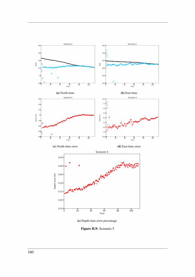
0 20 40 60 80 100Time
−20
0
20
40
60
80
North
Scenario 5
(a) North-time
0 20 40 60 80 100Time
−350
−340
−330
−320
−310
−300
East
Scenario 5
(b) East-time
0 20 40 60 80 100Time
−40
−30
−20
−10
0
10
20
30
North
erro
r
Scenario 5
(c) North-time error
0 20 40 60 80 100Time
−10.0
−7.5
−5.0
−2.5
0.0
2.5
5.0
7.5
10.0Ea
st erro
rScenario 5
(d) East-time error
0 20 40 60 80 100Time
−0.25
−0.20
−0.15
−0.10
−0.05
0.00
0.05
Depth error [%]
Scenario 5
(e) Depth-time error percentage
Figure H.9: Scenario 5
160
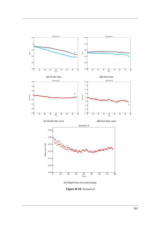
0 10 20 30 40 50 60 70 80Time
−40
−30
−20
−10
0
10
North
Scenario 6
(a) North-time
0 10 20 30 40 50 60 70 80Time
−350
−340
−330
−320
−310
−300
East
Scenario 6
(b) East-time
0 10 20 30 40 50 60 70 80Time
−40
−30
−20
−10
0
10
20
30
North
erro
r
Scenario 6
(c) North-time error
0 10 20 30 40 50 60 70 80Time
−10.0
−7.5
−5.0
−2.5
0.0
2.5
5.0
7.5
10.0Ea
st erro
rScenario 6
(d) East-time error
0 10 20 30 40 50 60 70 80Time
−0.25
−0.20
−0.15
−0.10
−0.05
0.00
0.05
Depth error [%]
Scenario 6
(e) Depth-time error percentage
Figure H.10: Scenario 6
161

Lina C. K. Theimann, Trine Ø
. Olsen
NTN
UN
orw
egia
n U
nive
rsity
of S
cien
ce a
nd T
echn
olog
yFa
culty
of I
nfor
mat
ion
Tech
nolo
gy a
nd E
lect
rical
Engi
neer
ing
Dep
artm
ent o
f Eng
inee
ring
Cybe
rnet
ics
Mas
ter’s
thes
is
Lina Charlotte Kristoffersen TheimannTrine Ødegård Olsen
Stereo vision for autonomous ferry
Master’s thesis in Cybernetics and Robotics
Supervisor: Edmund Førland Brekke,
Co-supervisor: Annette Stahl, Øystein K. Helgesen.
June 2020