Spatial chirp revisited: Matrix analysis of dispersionless optical

systems and correct interferometric autocorrelation

Nikolay Dimitrov, Nedyalko Chakarov, Alexander Dreischuh*

Department of Quantum Electronics, Faculty of Physics, Sofia University, 5, J. Bourchier Blvd., BG-1164 Sofia, Bulgaria

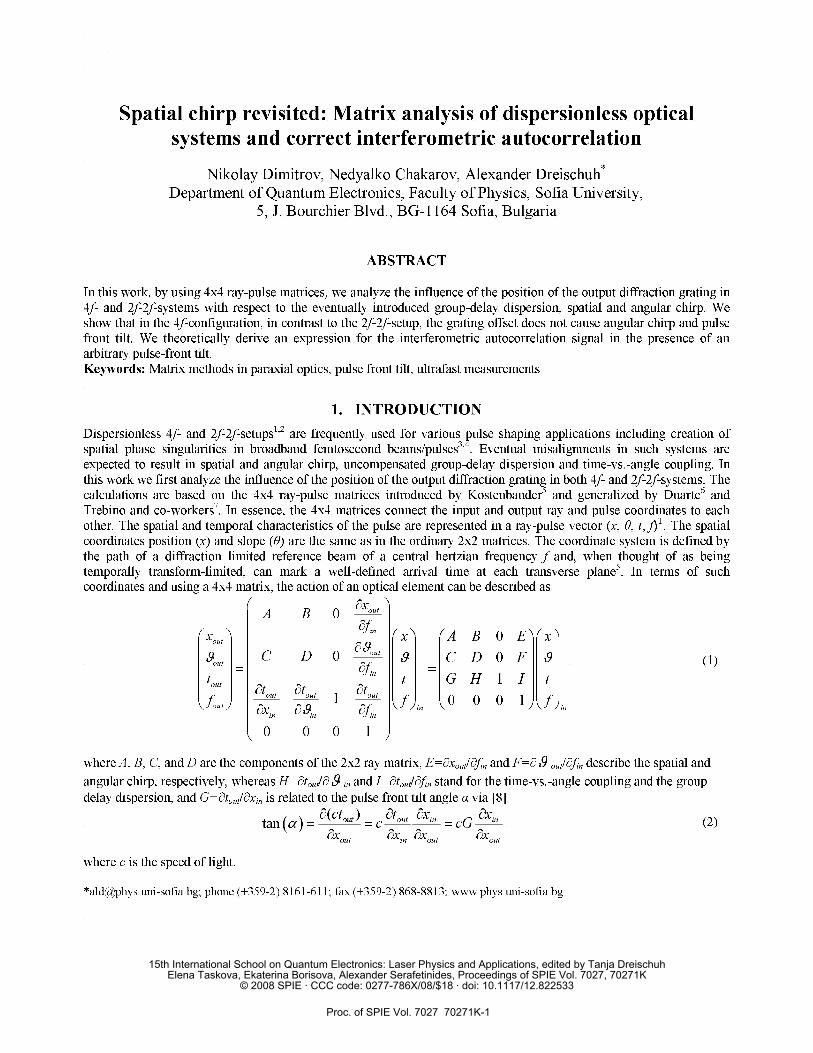
ABSTRACT

In this work, by using 4x4 ray-pulse matrices, we analyze the influence of the position of the output diffraction grating in

4f- and 2f-2f-systems with respect to the eventually introduced group-delay dispersion, spatial and angular chirp. We

show that in the 4f-configuration, in contrast to the 2f-2f-setup, the grating offset does not cause angular chirp and pulse

front tilt. We theoretically derive an expression for the interferometric autocorrelation signal in the presence of an

arbitrary pulse-front tilt.

Keywords: Matrix methods in paraxial optics, pulse front tilt, ultrafast measurements

1. INTRODUCTION

Dispersionless 4f- and 2f-2f-setups1,2

are frequently used for various pulse shaping applications including creation of

spatial phase singularities in broadband femtosecond beams/pulses3,4

. Eventual misalignments in such systems are

expected to result in spatial and angular chirp, uncompensated group-delay dispersion and time-vs.-angle coupling. In

this work we first analyze the influence of the position of the output diffraction grating in both 4f- and 2f-2f-systems. The

calculations are based on the 4x4 ray-pulse matrices introduced by Kostenbauder5 and generalized by Duarte

6 and

Trebino and co-workers7. In essence, the 4x4 matrices connect the input and output ray and pulse coordinates to each

other. The spatial and temporal characteristics of the pulse are represented in a ray-pulse vector (x, θ, t, f)T. The spatial

coordinates position (x) and slope (θ) are the same as in the ordinary 2x2 matrices. The coordinate system is defined by

the path of a diffraction limited reference beam of a central hertzian frequency f and, when thought of as being

temporally transform-limited, can mark a well-defined arrival time at each transverse plane5. In terms of such

coordinates and using a 4x4 matrix, the action of an optical element can be described as

0

0

0 0

1

1 0 0 0 1

0 0 0 1

out

in

out

out

out

in

out

out out out

out in in

in in in

xA B

fx x A B E x

C D C D Ff

t t G H I tt t t

f f fx f

ϑϑ ϑ ϑ

ϑ

∂⎛ ⎞⎜ ⎟∂⎜ ⎟⎛ ⎞ ⎛ ⎞ ⎛ ⎞⎛ ⎞⎜ ⎟∂⎜ ⎟ ⎜ ⎟ ⎜ ⎟⎜ ⎟⎜ ⎟⎜ ⎟ ⎜ ⎟ ⎜ ⎟⎜ ⎟∂= =⎜ ⎟⎜ ⎟ ⎜ ⎟ ⎜ ⎟⎜ ⎟⎜ ⎟∂ ∂ ∂⎜ ⎟ ⎜ ⎟ ⎜ ⎟⎜ ⎟⎜ ⎟⎝ ⎠ ⎝ ⎠⎝ ⎠⎝ ⎠ ∂ ∂ ∂⎜ ⎟⎜ ⎟⎝ ⎠

(1)

where A, B, C, and D are the components of the 2x2 ray matrix, E=∂xout/∂fin and F=∂ϑ out/∂fin describe the spatial and

angular chirp, respectively, whereas H=∂tout/∂ϑ in and I=∂tout/∂fin stand for the time-vs.-angle coupling and the group

delay dispersion, and G=∂tout/∂xin is related to the pulse front tilt angle α via [8]

( )( )

tan out out in in

out in out out

ct t x xc cG

x x x xα

∂ ∂ ∂ ∂= = =

∂ ∂ ∂ ∂

(2)

where c is the speed of light.

*ald@phys.uni-sofia.bg; phone (+359-2) 8161-611; fax (+359-2) 868-8813; www.phys.uni-sofia.bg

15th International School on Quantum Electronics: Laser Physics and Applications, edited by Tanja DreischuhElena Taskova, Ekaterina Borisova, Alexander Serafetinides, Proceedings of SPIE Vol. 7027, 70271K

© 2008 SPIE · CCC code: 0277-786X/08/$18 · doi: 10.1117/12.822533

Proc. of SPIE Vol. 7027 70271K-1

2. MATRIX ANALYSIS OF DISPERSIONLESS OPTICAL SYSTEMS

2.1 Analysis of a 4f-system

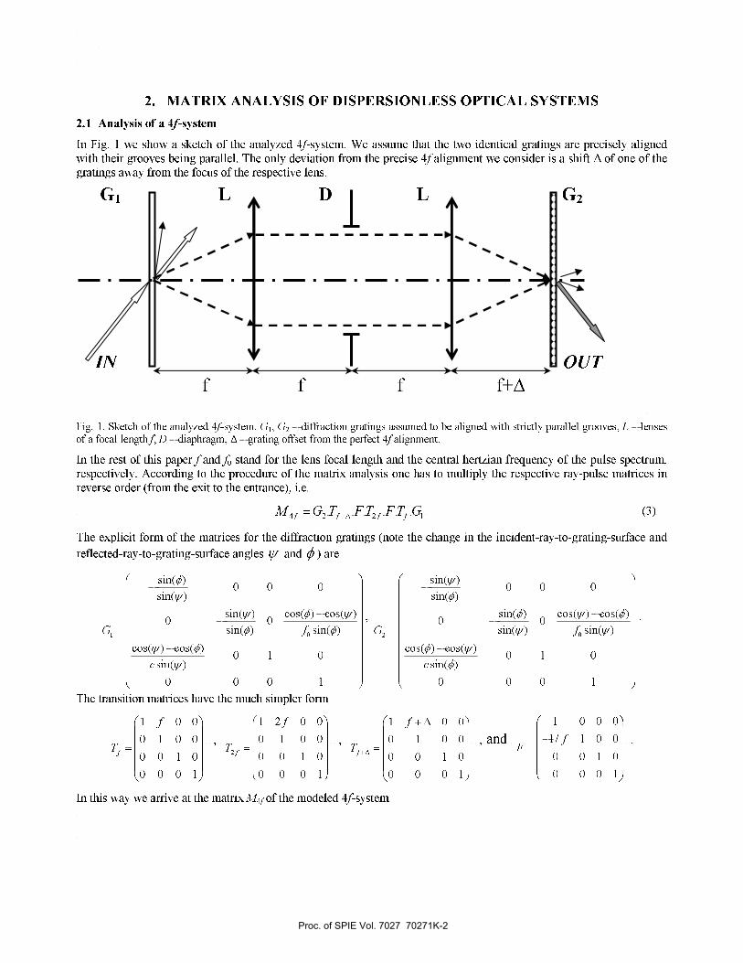
In Fig. 1 we show a sketch of the analyzed 4f-system. We assume that the two identical gratings are precisely aligned

with their grooves being parallel. The only deviation from the precise 4f alignment we consider is a shift Δ of one of the

gratings away from the focus of the respective lens.

Fig. 1. Sketch of the analyzed 4f-system. G1, G2 – diffraction gratings assumed to be aligned with strictly parallel grooves, L – lenses of a focal length f, D – diaphragm, Δ – grating offset from the perfect 4f alignment.

In the rest of this paper f and f0 stand for the lens focal length and the central hertzian frequency of the pulse spectrum,

respectively. According to the procedure of the matrix analysis one has to multiply the respective ray-pulse matrices in

reverse order (from the exit to the entrance), i.e.

4 2 2 1

. . . . . .f f f fM G T F T F T G+Δ

= (3)

The explicit form of the matrices for the diffraction gratings (note the change in the incident-ray-to-grating-surface and

reflected-ray-to-grating-surface angles ψ and φ ) are

01

sin( )0 0 0

sin( )

sin( ) cos( ) cos( )0 0

sin( ) sin( )

cos( ) cos( )0 1 0

sin( )

0 0 0 1

fG

c

φ

ψ

ψ φ ψ

φ φ

ψ φ

ψ

⎛ ⎞−⎜ ⎟

⎜ ⎟−⎜ ⎟

−⎜ ⎟= ⎜ ⎟⎜ ⎟−⎜ ⎟⎜ ⎟⎜ ⎟⎝ ⎠

,

02

sin( )0 0 0

sin( )

sin( ) cos( ) cos( )0 0

sin( ) sin( )

cos( ) cos( )0 1 0

sin( )

0 0 0 1

fG

c

ψ

φ

φ ψ φ

ψ ψ

φ ψ

φ

⎛ ⎞−⎜ ⎟

⎜ ⎟−⎜ ⎟

−⎜ ⎟= ⎜ ⎟⎜ ⎟−⎜ ⎟⎜ ⎟⎜ ⎟⎝ ⎠

.

The transition matrices have the much simpler form

1 0 0

0 1 0 0

0 0 1 0

0 0 0 1

f

f

T

⎛ ⎞⎜ ⎟⎜ ⎟=⎜ ⎟⎜ ⎟⎝ ⎠

,

2

1 2 0 0

0 1 0 0

0 0 1 0

0 0 0 1

f

f

T

⎛ ⎞⎜ ⎟⎜ ⎟=⎜ ⎟⎜ ⎟⎝ ⎠

,

1 0 0

0 1 0 0

0 0 1 0

0 0 0 1

f

f

T+Δ

+ Δ⎛ ⎞⎜ ⎟⎜ ⎟=⎜ ⎟⎜ ⎟⎝ ⎠

, and

1 0 0 0

1/ 1 0 0

0 0 1 0

0 0 0 1

fF

⎛ ⎞⎜ ⎟−⎜ ⎟=⎜ ⎟⎜ ⎟⎝ ⎠

.

In this way we arrive at the matrix M4f of the modeled 4f-system

f f f f+Δ

G1 L D G2 L

IN OUT

Proc. of SPIE Vol. 7027 70271K-2

( )

( ) ( )

2

2 2

0

4 2

2

0

cos( ) cos( ) sin( )sin ( )1 0

sin ( ) sin ( )

0 1 0 0

cos( ) cos( ) sin( ) cotg( ) cos( ) / sin( )0 1

sin ( )

0 0 0 1

f

f

M

c cf

φ ψ ψψ

φ φ

φ ψ ψ φ ψ φ

φ

⎛ ⎞−− −Δ Δ⎜ ⎟

⎜ ⎟⎜ ⎟−⎜ ⎟=⎜ ⎟− −

Δ −Δ⎜ ⎟⎜ ⎟⎜ ⎟⎝ ⎠

. (4)

It is evident that the misalignment Δ of the grating determines the signs of the introduced group-delay dispersion (GDD),

spatial chirp (SC) and time-vs.-angle coupling (TvAC):

( )2

0

cotg( ) cos / sin( )out

in

tGDD

f cfφ ψ φ

∂ Δ⎡ ⎤= = − −⎣ ⎦∂

, (5a)

( )

2

0

cos( ) cos sin( )

sin ( )

out

in

xSC

f f

φ ψ ψ

φ

⎡ ⎤Δ −∂ ⎣ ⎦= =∂

, (5b)

[ ]

2

cos( ) cos( ) sin( )v

sin ( )

out

in

tT AC

c

φ ψ ψ

ϑ φ

−∂= = Δ∂

. (5c)

Since in M4f (see Eq. 4) the matrix elements F=0 and G=0, this misalignment does not introduce angular chirp and pulse

front tilt.

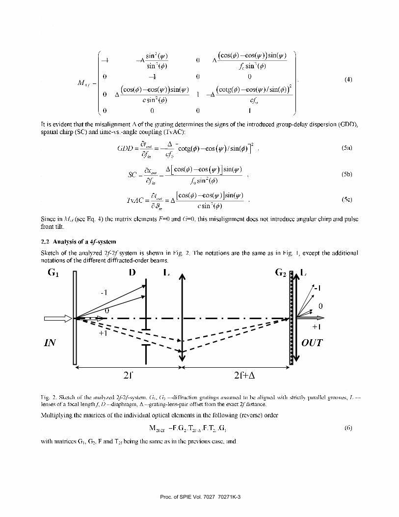
2.2 Analysis of a 4f-system

Sketch of the analyzed 2f-2f system is shown in Fig. 2. The notations are the same as in Fig. 1, except the additional notations of the different diffracted-order beams.

Fig. 2. Sketch of the analyzed 2f-2f-system. G1, G2 – diffraction gratings assumed to be aligned with strictly parallel grooves, L – lenses of a focal length f, D – diaphragm, Δ – grating-lens-pair offset from the exact 2f distance.

Multiplying the matrices of the individual optical elements in the following (reverse) order

2f-2f 2 2f+ 2f 1

M =F.G .T .F.T .GΔ

(6)

with matrices G1, G2, F and T2f being the same as in the previous case, and

OUT

2f 2f+Δ

G1 L D G2 L

IN

0

+1

-1

0

+1

-1

Proc. of SPIE Vol. 7027 70271K-3

2

1 2 0 0

0 1 0 0

0 0 1 0

0 0 0 1

f

f

T+Δ

+Δ⎛ ⎞⎜ ⎟⎜ ⎟=⎜ ⎟⎜ ⎟⎝ ⎠

we derive the matrix M2f-2f of the misaligned 2f-2f system

( )

( )

( ) ( )

2 2

2

2 2

0

2 2 2

2 2

0

2

cos( ) cos( ) sin( )sin ( )0

sin ( ) sin ( )

cotg( ) cos( ) / sin( ) sin( )sin ( ) / sin ( ) sin ( )1 0

sin ( ) sin( )

cotg( ) cos( ) / sin( ) cos( ) cos( ) sin( ) cotg(1

sin ( )

f fM

f

f f

f f

f f ff

cf c

φ ψ ψψ

φ φ

φ ψ φ ψφ ψ ψ

φ φ

ψ φ ψ φ ψ ψ φ

φ

−

=

−Δ +− −Δ Δ

−Δ + −− +Δ −Δ

− −−Δ Δ −Δ

( )2

0

) cos( ) / sin( )

0 0 0 1

cf

ψ φ

⎛ ⎞⎜ ⎟⎜ ⎟⎜ ⎟⎜ ⎟⎜ ⎟⎜ ⎟

−⎜ ⎟⎜ ⎟⎜ ⎟⎜ ⎟⎝ ⎠

. (7)

As seen, in this case the grating-lens-pair misalignment has much more complicated consequences. Comparing Eqs. 4

and 7 one can see that equal misalignments of the systems result in equal group-delay dispersion (GDD, Eq. 5a), spatial

chirp (SC, Eq. 5b) and time-vs.-angle coupling (TvAC, Eq. 5c). The misalignment introduces however a pulse-front-tilt

(PFT)

cotg( ) cos( ) / sin( )

out

in

tPFT

x cf

ψ φ ψ∂ −= = −Δ∂

. (8)

This later pulse distortion, which is especially important for nearly single-cycle ultrashort optical pulses, is understood8

as an arrival time difference out

t which depends on the transverse beam coordinate outx . In a misaligned 2f-2f-system

the corresponding pulse front tilt angle α is given by

[ ]( )

tan( ) cotg( ) cos( ) / sin( )out out in

out in out

ct t xc

x x x fα ψ φ ψ

∂ ∂ ∂ Δ= = = −

∂ ∂ ∂ + Δ

. (9)

3. AUTOCORRELATION SIGNAL IN THE PRESENCE OF PULSE FRONT TILT

In this section we consider Gaussian beam/pulse of width x0 and duration t0. When there is no pulse front tilt, the electric

field of this wave is described by

( ) ( ) ( )2 2

0 0 0( , ) exp / / expE x t E x x t t i tω⎡ ⎤= − −

⎣ ⎦ . (10)

Fig. 3 is intended to visualize the difference between pulses without and with pulse front tilt. The right frame in Fig. 3

correctly corresponds to the understanding that, at a fixed plane perpendicular to the beam propagation direction, an

arrival time difference depending on the transverse beam coordinate means presence of a spatial chirp. In a standard

Michelson-type autocorrelator the pulse front tilt remains hidden [9] (see Fig. 4, left). The picture drastically changes

when one of the beams is rotated in space at 180o (Fig. 4, right). Setups for an interferometric inverted field

autocorrelation suited for the detection of tilted pulse fronts are known9,10

. Our goal in this section is to derive an analytic

expression for the interferometric autocorrelation signal for arbitrary large pulse front tilt.

Starting with the optical field amplitudes E1 and E2 of the beams/pulses with opposite pulse front tilts -α and α,

respectively, the intensity I2ω of the second harmonic that is generated during the autocorrelation is

Proc. of SPIE Vol. 7027 70271K-4

Fig. 3. Electric field amplitude of an ultrashort pulse without (left) and with pulse front tilt (right).

Fig. 4. Electric field amplitude of an ultrashort pulse with pulse front tilt propagating in a standard Michelson-type autocorrelator (left) and in an autocorrelator, in which one of the beams is rotated in space at 180o (right).

( ) ( ) ( )2

2 2

2 2 1 2, , , , , , ( , , ) ( , , , )

d d dI x t E x t E x t E x tω ω

α τ α τ α α τ= = − + . (11)

τd is the time delay between the pulses during the autocorrelation. With a wide aperture photodetector and a detector rise

time much longer than the typical pulse length (conditions easily fulfilled with ultrashort pulses) the normalized

correlation signal has the form

( )( )

( )

2

2 22

, , ,,

2 ( , , , )

dAK

d

i d

I x t dxdt

P

E x t dxdt

ω

ω

α τ

α τ

α τ

∞ ∞

−∞ −∞

∞ ∞

−∞ −∞

=

∫ ∫

∫ ∫ , (12)

where i=1,2. The natural normalization to the energy of the second harmonic signal generated from each pulse separately

yields a correlation peak-to-background ratio of 8:1 at zero tilt of the pulse front. The most time-consuming but

straightforward step in this analysis is the correct rotation of the electric field amplitude (10) at an angle -α and α,

respectively. Following the procedure described above, we derived general expression for the interferometric

autocorrelation signal for arbitrary large pulse front tilt α

- 10 - 5 0 5 10 15

x

- 7.5

- 5

- 2.5

0

2.5

5

7.5

10

t

- 10 - 5 0 5 10 15

x

- 7.5

- 5

- 2.5

0

2.5

5

7.5

10

t

- 7.5 - 5 - 2.5 0 2.5 5 7.5 10

x

- 6

- 4

- 2

0

2

4

6

t

- 7.5 - 5 - 2.5 0 2.5 5 7.5 10

x

- 6

- 4

- 2

0

2

4

6

t

Proc. of SPIE Vol. 7027 70271K-5

( )2 2

2 0 0

( ) 18exp [ ] exp 2 [2 ]

( ) ( )( , ) 1 2 2

( ) ( )

d d d d

AK

d

Acos cos

B CP x t

B Dω

α

τ ωτ τ ωτ

α α

α τ

α α

⎛ ⎞⎧ ⎫ ⎧ ⎫⎪ ⎪ ⎪ ⎪ ⎟⎪ ⎪ ⎪ ⎪⎜ ⎟− − +⎜ ⎨ ⎬ ⎨ ⎬ ⎟⎜ ⎟⎪ ⎪ ⎪ ⎪⎜ ⎟⎪ ⎪ ⎪ ⎪⎩ ⎭ ⎩ ⎭⎜ ⎟= + +⎜ ⎟⎜ ⎟⎟⎜ ⎟⎜ ⎟⎜ ⎟⎜⎝ ⎠

, (13)

where

2 2 2 2

0 0 0 0

4 2 2 4 2 2 2

0 0 0 0 0 0

2 2 2 2

0 0

4 2 2 4 2 2 2

0 0 0 0 0 0

( ) 12 ( ) ( ) (2 )

( ) 3 26 3 3( ) (4 )

( ) ( ) ( )

( ) 6 ( ) (4 )

A x t x t cos

B x x t t x t cos

C t cos x sin

D x x t t x t cos

α α

α α

α α α

α α

⎡ ⎤= + + −⎢ ⎥⎣ ⎦

= + + − −

= +

= + + − −

. (14)

In Fig. 5 we show numerically calculated interferometric autocorrelation signals 2

AKPω

for different values of α. It is

evident that the correlation peak-to-background signal ratio of 8:1 for α=0 gradually decreases with increasing α,

whereas the amplitudes of the side lying peaks grow monotonically. This is a clear indication that the autocorrelation curve broadens with increasing the pulse front tilt. The effect is better pronounced when we inspect the envelopes of the

autocorrelation signals (see Fig. 6). It is intuitively clear that, at one and the same beam width, the shorter the laser pulse,

the stronger the influence of the pulse front tilt. Table 1 summarizes results concerning the relative pulse broadening

Δt/Δt(α=0) for different pulse duration to beam width ratios vs. tilt angle α. As seen, for α=0.35rad a decrease of the

pulse duration by a factor of 3 results in an increase of the effective pulse broadening by a factor of more than 2. The

shorter pulses appear stronger influenced by the pulse front tilt α than the longer ones.

-16 -12 -8 -4 0 4 8 12 16

0

2

4

6

8

τd

PAK

2ω

t0=4; x

0=16

α, rad

0

0.05

0.15

0.25

0.35

Fig. 5. Simulated interferometric atocorrelation signal (Eq. 13) for different values of the pulse front tilt α.

Proc. of SPIE Vol. 7027 70271K-6

-16 -12 -8 -4 0 4 8 12 16

0

2

4

6

8

α=0.0

0.05

0.1

0.15

0.2

0.25

0.3

0.35

Envelope of P

AK

2ω

τd

t0=4; x

0=16;

Fig. 6. Simulated envelopes of the interferometric atocorrelation signals (Eq. 13) for different values of the pulse front tilt α.

-16 -12 -8 -4 0 4 8 12 16

0

2

4

6

8t0=6; x

0=16;

τd

PAK

2ω

exact

approximate

deviation

α =0.1rad

Fig. 7. Simulated interferometric atocorrelation signals by using the exact (Eq. 13) and the approximate analytical result (Eq. 15) and difference of the calculated signals (bottom curve) for pulse front tilt α=0.1rad.

Proc. of SPIE Vol. 7027 70271K-7

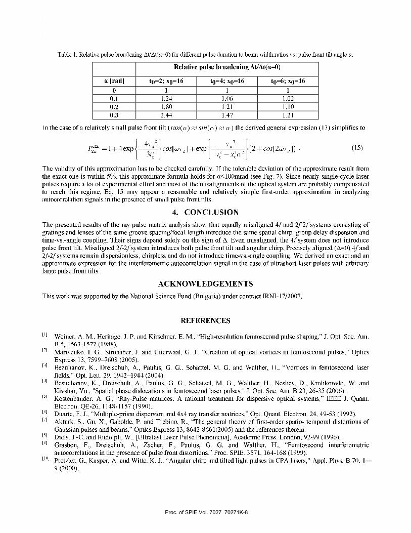
Table 1. Relative pulse broadening Δt/Δt(α=0) for different pulse duration to beam width ratios vs. pulse front tilt angle α.

Relative pulse broadening Δt/Δt(α=0)

α [rad] t0=2; x0=16 t0=4; x0=16 t0=6; x0=16

0 1 1 1

0.1 1.24 1.06 1.02

0.2 1.80 1.21 1.10

0.3 2.44 1.47 1.21

In the case of a relatively small pulse front tilt ( ( ) ( )tan sinα α α≈ ≈ ) the derived general expression (13) simplifies to

( )2 2

2 2 2 2 2

0 0 0

41 4exp [ ] exp 2 [2 ]

3

AK d d

d dP cos cos

t t xω

τ τ

ωτ ωτ

α

⎧ ⎫ ⎧ ⎫⎪ ⎪ ⎪ ⎪⎪ ⎪ ⎪ ⎪= + − + − +⎨ ⎬ ⎨ ⎬⎪ ⎪ ⎪ ⎪+⎪ ⎪ ⎪ ⎪⎩ ⎭ ⎩ ⎭

. (15)

The validity of this approximation has to be checked carefully. If the tolerable deviation of the approximate result from

the exact one is within 5%, this approximate formula holds for α<100mrad (see Fig. 7). Since nearly single-cycle laser

pulses require a lot of experimental effort and most of the misalignments of the optical system are probably compensated

to reach this regime, Eq. 15 may appear a reasonable and relatively simple first-order approximation in analyzing autocorrelation signals in the presence of small pulse front tilts.

4. CONCLUSION

The presented results of the ray-pulse matrix analysis show that equally misaligned 4f and 2f-2f systems consisting of

gratings and lenses of the same groove spacing/focal length introduce the same spatial chirp, group delay dispersion and

time-vs.-angle coupling. Their signs depend solely on the sign of Δ. Even misaligned, the 4f system does not introduce

pulse front tilt. Misaligned 2f-2f system introduces both pulse front tilt and angular chirp. Precisely aligned (Δ=0) 4f and

2f-2f systems remain dispersionless, chirpless and do not introduce time-vs.-angle coupling. We derived an exact and an approximate expression for the interferometric autocorrelation signal in the case of ultrashort laser pulses with arbitrary

large pulse front tilts.

ACKNOWLEDGEMENTS

This work was supported by the National Science Fund (Bulgaria) under contract IRNI-17/2007.

REFERENCES

[1] Weiner, A. M., Heritage, J. P. and Kirschner, E. M., “High-resolution femtosecond pulse shaping,” J. Opt. Soc. Am.

B 5, 1563-1572 (1988). [2]

Mariyenko, I. G., Strohaber, J. and Uiterwaal, G. J., “Creation of optical vortices in femtosecond pulses,” Optics

Express 13, 7599–7608 (2005). [3]

Bezuhanov, K., Dreischuh, A., Paulus, G. G., Schätzel, M. G. and Walther, H., “Vortices in femtosecond laser

fields,” Opt. Lett. 29, 1942–1944 (2004). [4]

Besuchanov, K., Dreischuh, A., Paulus, G. G., Schätzel, M. G., Walther, H., Neshev, D., Krolikowski, W. and

Kivshar, Yu., "Spatial phase dislocations in femtosecond laser pulses," J. Opt. Soc. Am. B 23, 26-35 (2006). [5]

Kostenbauder, A. G., “Ray-Pulse matrices: A rational treatment for dispersive optical systems,” IEEE J. Quant.

Electron. QE-26, 1148-1157 (1990). [6]

Duarte, F. J., “Multiple-prism dispersion and 4x4 ray transfer matrices,” Opt. Quant. Electron. 24, 49-53 (1992). [7]

Akturk, S., Gu, X., Gabolde, P. and Trebino, R., “The general theory of first-order spatio- temporal distortions of

Gaussian pulses and beams,” Optics Express 13, 8642-8661(2005) and the references therein. [8]

Diels, J.-C. and Rudolph, W., [Ultrafast Laser Pulse Phenomena], Academic Press, London, 92-99 (1996). [9]

Grasbon, F., Dreischuh, A., Zacher, F., Paulus, G. G. and Walther, H., “Femtosecond interferometric

autocorrelations in the presence of pulse front distortions,” Proc. SPIE, 3571, 164-168 (1999). [10]

Pretzler, G., Kasper, A. and Witte, K. J., “Angular chirp and tilted light pulses in CPA lasers,” Appl. Phys. B 70, 1–

9 (2000).

Proc. of SPIE Vol. 7027 70271K-8