Testing Spatial Autocorrelation in WeightedNetworks: the Modes Permutation Test

Francois Bavaud

Department of Computer Science and Mathematical MethodsDepartment of Geography

University of Lausanne, Switzerland

Abstract. In a weighted spatial network, as specified by an exchangematrix, the variances of the spatial values are inversely proportional tothe size of the regions. Spatial values are no more exchangeable under in-dependence, thus weakening the rationale for ordinary permutation andbootstrap tests of spatial autocorrelation. We propose an alternativepermutation test for spatial autocorrelation, based upon exchangeablespatial modes, constructed as linear orthogonal combinations of spatialvalues. The coefficients obtain as eigenvectors of the standardised ex-change matrix appearing in spectral clustering, and generalise to theweighted case the concept of spatial filtering for connectivity matrices.Also, two proposals aimed at transforming an acessibility matrix into aexchange matrix with with a priori fixed margins are presented. Two ex-amples (inter-regional migratory flows and binary adjacency networks)illustrate the formalism, rooted in the theory of spectral decompositionfor reversible Markov chains.

Keywords: bootstrap, local variance, Markov and semi-Markov processes, Moran’s I,permutation test, spatial autocorrelation, spatial filtering, weighted networks

1 Introduction

Bavaud, F. Testing Spatial Autocorrelation in Weighted Networks: the Modes Permutation

Test. Journal of Geographical Systems, July 2013, Volume 15, Issue 3, pp 233–247. DOI:

10.1007/s10109-013-0179-2, http://link.springer.com/article/10.1007%2Fs10109-013-0179-2

Permutation tests of spatial autoccorelation are justified under exchangeabil-ity, that is the premise that the observed scores follow a permutation-invariantjoint distribution. Yet, in the frequently encountered case of geographical datacollected on regions differing in importance, the variance of a regional score is ex-pected to decrease with the size of the region, in the same way that the varianceof an average is inversely proportional to the size of the sample in elementarystatistics: heteroscedasticity holds in effect, already under spatial independence,thus weakening the rationale of the celebrated spatial autocorrelation permu-tation test (e.g. Cliff and Ord 1973; Besag and Diggle 1977) in the case of aweighted network.

This paper presents an alternative permutation test for spatial autocorre-lation, whose validity extends to the weighted case. The procedure relies uponspatial modes, that is linear orthogonal combinations of spatial values, originally

2

based upon the eigenvectors of the standardized connectivity or adjacency ma-trix (Tiefelsdorf and Boots 1995; Griffth 2000). In contrast to regional scores,the variance of the spatial modes turn out to be constant under spatial indepen-dence, thereby justifying the modes permutation test for spatial autocorrelation.

Section 2.1 presents the definition of the local variance and Moran’s I in thearguably most general setup for spatial autocorrelation, based upon the nor-malised, symmetrical exchange matrix, whose margins define regional weights(Bavaud 2008a). Section 2.2 presents, in the spirit of spatial filtering (Griffth2000), the spectral decomposition of the exchange matrix, or rather of a stan-dardised version of it, currently used in spectral graph theory (Chung 1997; vonLuxburg 2007; Bavaud 2010), supplying the orthogonal components defining inturn the spatial modes. Section 2.3 presents the mode permutation test, and itsbootstrap variant, illustrated in section 2.4 on Swiss migratory and linguisticdata.

Section 3 addresses the familiar case of binary or weighted adjacency matri-ces, which have to be first converted into exchange matrices with a priori fixedmargins. Two proposals, namely a simple rescaling with diagonal adjustment(Section 3.1) and the construction of time-embeddable exchange matrices (Sec-tion 3.2) are presented, and illustrated on the popular “distribution of Bloodgroup A in Eire” dataset (Section 3.3).

2 Spatial autocorrelation in weighted netwoks

2.1 Local covariance and the exchange matrix

Consider a set of n regions with associated weights fi > 0, normalized to∑ni=1 fi = 1. Weights measure the importance of the regions, and define weighted

regional averages and variances as

x :=

n∑i=1

fixi var(x) :=

n∑i=1

fi(xi − x)2 =1

2

∑ij

fifj(xi − xj)2 . (1)

Here x = (xi) represents a density variable or a spatial field, that is a numericalquantity attached to region i, transforming under aggregation i, j → [i ∪ j] asx[i∪j] = (fixi + fjxj)/(fi + fj), as for instance “cars per inhabitants”, “averageincome” or “proportion of foreigners”.

The last identity in (1) is straightforward to check (Lebart 1969), and showsthe variance to measure the average squared dissimilarity between pairs (i, j) ofregions, selected independently with probability fifj . A more general samplingscheme consists in selecting the regional pair (i, j) with probability eij , such that

eij ≥ 0 eij = eji ei• :=∑j

eij = fi e•• = 1 (2)

where ”•” denotes the summation over the replaced index. A n × n matrixE = (eij) obeying (2) is called an exchange matrix (Berger and Snell 1957;

3

Bavaud 2008a), compatible with the regional weights f . The exchange matrixdefines an undirected weighted network, with edges weights eij and regionalweights fi = ei•. It contains loops in general (eii ≥ 0), denoting regional self-interaction or autarachy (Bavaud 1998).

By construction, the exchange matrix generates a reversible Markov transi-tion matrix W = (wij) (Bavaud 1998) with stationary distribution f :

wij :=eijfi≥ 0

∑j

wij = 1∑i

fiwij = fj fiwij = fjwji = eij . (3)

W constitutes a row-normalized matrix of spatial weights, entering in the au-toregressive models of spatial econometrics (see e.g. Anselin 1988; Cressie 1993;Leenders 2002; Haining 2003; Arbia 2006; LeSage and Pace 2009).

In spatial applications, the components of the exchange matrix are large fornearby regions and small for regions far apart. The quantity

varloc(x) :=1

2

∑ij

eij(xi − xj)2 (4)

defines the local variance, that is the average squared dissimilarity between neigh-bours. Comparing the local and the ordinary (weighted) variance defines Geary’sc and Moran’s I, measuring spatial autocorrelation (e.g. Geary 1954; Moran1950 ; Cliff and Ord 1973; Tiefelsdorf and Boots 1995; Anselin 1995). Namely,c(x) := varloc(x)/var(x) (differing from its usual variant by a factor n/(n − 1))and

I(x) := 1− c(x) =var(x)− varloc(x)

var(x)=

∑ij eij(xi − x)(xj − x)∑

i fi(xi − x)2.

2.2 Spatial filtering and spatial modes

Spatial filtering primarily aims at visualizing and extracting the latent factors in-volved in spatial autocorrelation (Tiefelsdorf and Boots 1995; Griffith 2000, 2003;Griffith and Peres-Neto 2006; Chun 2008; Dray 2011; and references therein).

Its first step consists in spectrally decomposing a matrix expressing inter-regional connectivity in some way or another, such as the adjacency matrix or theexchange matrix. Various choices are often equivalent under uniform weightingof the regions, but the general weighted case calls for more precision. Arguably,the most fruitful decomposition considers the so-called standardized exchangematrix Es, with components (Chung 1997, von Luxburg 2007; Bavaud 2010)

esij =eij − fifj√

fifji.e. Es = Π−

12 (E − ff ′)Π− 1

2 with Π = diag(f) . (5)

Its spectral decomposition

Es = UΛU ′ with U = (uiα) orthogonal and Λ = diag(λ) diagonal

4

generates a trivial eigenvalue λ0 = 0 associated with the trivial eigenvectorui0 =

√fi. The remaining non-trivial decreasingly ordered eigenvalues λα (for

α = 1, . . . , n − 1) lie in the interval [−1, 1], as a consequence of the Perron-Froebenius theorem and the symmetry of Es.

Also, λ1 = 1 iff E is reducible, that is consisting of two or more disconnectedcomponents (Figure 1), and λn−1 = −1 iff E is bipartite, i.e. partitionable intotwo sets without within connections (e.g. Kijima 1997; Aldous and Hill 2002).

Fig. 1. Reducible network, with λ1 = 1 (left) and bipartite network, with λn−1 = −1(right)

The exchange matrix itself expresses as

eij = fifj +√fifj

n−1∑α=1

λαuiαujα = fifj [1 +∑α≥1

λαciαcjα] (6)

where the raw coordinates

ciα :=uiαui0

=uiα

±√fi

can be used at visualizing distinct levels of spatial autocorrelation (Griffith 2003),or at specifying the positions of the n regions in a factor space (Bavaud 2010).

Raw coordinates are orthogonal and standardized, in the sense∑i

ficiα = δα0∑i

ficiαciβ = δαβ . (7)

As a consequence, the n regional values x can be converted into n modal valuesx, and vice-versa, as

xα :=∑i

ficiαxi xi =∑α≥0

ciαxα = x+∑α≥1

ciαxα . (8)

Equations (8) express orthogonal, Fourier-like correspondence between regionalvalues and modes. The latter depict global patterns, integrating the contributionsfrom all regions. In particular, the trivial mode yields the field average: x0 = x.

Borrowing an analogy from solid-state Physics, the spatial field x can describethe individual displacements of each of the n atoms of a crystal. The modes x

5

then provide global parameters describing the collective motion of atoms, con-sisting of a superposition of sound waves or harmonics, whose specific eigen-frequencies are determined by the nature of the crystal, and whose knowledgepermit to reconstruct the individual atomic displacements.

2.3 The modes permutation test

2.3.1 Heterodasticity of the spatial field The hypothesis H0 of spatial in-dependence requires the covariance matrix of the spatial field X = (X1, . . . , Xn)to be diagonal with components inversely proportional to the spatial weights,that is of the form (see the Appendix)

σij = Cov(Xi, Xj) = δijσ2

fiwhere σ2 = Var(X) . (9)

In its usual form, the direct or regional permutation test compares the ob-served value of Moran’s I(x) to a set of values I(π(x)), where π(x) denotes apermutation (that is a sampling without replacement) of the n regional valuesx (e.g. Cliff and Ord 1973; Thioulouse et al. 1995; Li and al. 2007; Bivand et al.2009a). Sampling with replacement, generating bootstrap resamples can also becarried out.

Both procedures are justified by the fact that the spatial variables Xi areidentically distributed under H0. Yet, (9) shows the latter assertion to be wrongwhenever the regional weights differ, thus jeopardizing the rationale of the directapproach, based upon the permutation or the bootstrap of regional values.

The possible heteroscedasticity of regional values has been addressed by quitea few researchers, in particular in epidemiology, and various proposals (transfor-mations of variables or weights, reformulations in terms of residuals, Bayesianapproaches) have been investigated (see e.g. Waldhor 1996, Assuncao and Reis1999 or Haining 2003).

2.3.2 Homoscedasticity of the spatial modes As annouced in the intro-duction, this paper proposes a presumably new modal test, identical in spirit tothe direct test but based upon modes permutation, together with a variant basedupon modes bootstrap. Its existence results from two fortunate circumstances (seethe Appendix), namely i) the homoscedasticity of the modes under H0

σαβ := Cov(Xα, Xβ) = δαβ σ2 with Xα =

∑i

fi ciα Xi (10)

and ii) the simplicity of Moran’s I expression in terms of spatial modes, whichreads

I(x) ≡ I(x) =

∑α≥1 λαx

2α∑

α≥1 x2α

. (11)

As expected, the trivial mode x0 = x does not contribute to Moran’s I. UnderH0, its expectation and variance under all remaining (n− 1)! non-trivial modes

6

permutations read (see the Appendix)

Eπ(I | x) =1

n− 1

∑α≥1

λα =trace(W )− 1

n− 1≥ −1

n− 1(12)

Varπ(I | x) =s(x)− 1

(n− 1)(n− 2)[∑α≥1

λ2α −1

n− 1(∑α≥1

λα)2] (13)

where

s(x) := (n− 1)

∑α≥1 x

4α

(∑α≥1 x

2α)2≥ 1

is a measure of modes dispersion.

2.3.3 The test The modes autocorrelation test consists in refuting H0, whichdenies spatial dependence, if the value (11) of I(x) is extreme w.r.t. the sample{I(π(x))} of B permuted or boostrapped mode values, that is if its quantile isnear 1 (evidence of positive autocorrelation) or near 0 (negative autocorrelation).

As expected, the trivial mode x0 = x does not contribute to Moran’s I.Also, I(x) together with its permuted or boostrapped values lie in an intervalcomprised in [λn−1, λ1] ⊆ [−1, 1]. The interval reduces to a single point I(π(x)) ≡I0, invariant under permutations or boostraping, with a corresponding variance(13) of zero, thus ruining the autocorrelation test, if (see 11, 13):

a) s(x) = 1, that is x2α ≡ x2 or equivalently xα ≡ εα x, where x ∈ R andεα = ±1 for all α ≥ 1. Following (8), this occurs for “untestable” spatialfields of the form xi = x + xzi where zi =

∑α≥1 εαuiα/ui0 actually defines

a set of 2n−1 configurations depending on the choice of the εα, whose sign isarbitrary, as is the sign of the eigenvectors uα.Noticeably, the constant field xi ≡ x is untestable, with a value I(x) =0/0 not even defined. However intriguing, the empirical relevance of those“untestable” spatial fields is debatable, in view of the vanishing probabilityto encounter exactly such a spatial pattern.

b) λα ≡ λ for all α ≥ 1, as with the :

i) frozen networks E := E(0), where e(0)ij := fiδij is the disconnected

graph1, associated to the immobile Markov chain with λα ≡ 1 andI(x) ≡ 1 (Figure 2 left)

ii) or as with the perfectly mobile networks E := E(∞), where e(∞)ij :=

fifj is the complete weighted graph, free of distance-deterrence effects,associated to the memoryless Markov chain with λα ≡ 0 and I(x) ≡ 0(Figure 2 middle)

1 Here the notations match the higher-order discrete time extensions of the exchangematrix, resulting (under weak regularity conditions) from the iteration of the Markovtransition matrix as

E(r) := ΠW r E(0) = Π E(2) = EΠ−1E E(∞) = ff ′ .

7

as well as with their linear combinations E := aE(0) + (1 − a)E(∞). Also,networks made of n = 2 regions are untestable: they automatically satisfyb) and a) above (Figure 2 right).

Under the additional normal assumption Xα ∼ N(0, σ2) for α ≥ 1, one canshow E(s(x)) = 3(n − 1)/(n + 1) by the Pitman-Koopmans theorem (Cliff andOrd 1981 p.43) and hence

E(Varπ(I | x)) =2

n2 − 1[∑α≥1

λ2α −1

n− 1(∑α≥1

λα)2]

=2

n2 − 1[tr(W 2)− 1− (tr(W )− 1)2

n− 1] . (14)

Fig. 2. Moran’s I(x) is constant, independent of the value of the field x for the dis-connected or frozen network (left), for the fully connected or perfectly mobile network(middle), and their linear combinations. Its minimum I(x) ≡ −1 occurs for the looplessnetwork with n = 2 (right).

2.4 Illustration: Swiss migratory and linguistic data

Flows constitute a major source of exchange matrices (e.g. Goodchild and Smith1980; Willekens J. 1983; Fotheringham and O’Kelly, M.E. 1989; Sen and Smith1995; Bavaud 1998, 2002). Let nij(T ) denote the number of units (people, goods,matter, etc.) initially in region i and located in region j after a time T . Quasi-symmetric flows are of the form nij = aibjcij with cij = cji, as predicted byGravity modelling. They generate reversible spatial weights wij := nij/ni•, withstationary distribution fi, whose product fiwij defines the exchange matrix eij(Bavaud 2002).

Consider the inter-regional migrations data nij(T ) between the n = 26 Swisscantons for T = 5 years (1985-90), together with the spatial fields x = “proportionof germanophones” or x = “proportion of anglophones”, for each canton. Afterdetermining the quasi-symmetric ML estimates nij (Bavaud 2002), the exchangematrix is computed, and so are the spatial modes xα from (8) and Moran’s

8

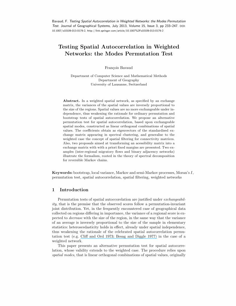
index I(x) from (11). Figure 3 depicts the distribution of 10′000 permutationand boostrap resamples of I(π(x)), from which the bilateral p-values of Table 1can be computed (see Section 3.2 for the details).

values of Moran's I(x) for x=proportion of germanophones

Modal (red) and direct (blue) sampling, without replacement

density

0.84 0.86 0.88 0.90 0.92 0.94 0.96 0.98

010

20

30

40

50

0.84 0.86 0.88 0.90 0.92 0.94 0.96 0.98

010

20

30

40

50

values of Moran's I(x) for x=proportion of anglophones

Modal (red) and direct (blue) sampling, without replacement

density

0.84 0.86 0.88 0.90 0.92 0.94 0.96 0.980

10

20

30

40

50

0.84 0.86 0.88 0.90 0.92 0.94 0.96 0.980

10

20

30

40

50

values of Moran's I(x) for x=proportion of germanophones

Modal (red) and direct (blue) sampling, with replacement

density

0.84 0.86 0.88 0.90 0.92 0.94 0.96 0.98

010

20

30

40

50

0.84 0.86 0.88 0.90 0.92 0.94 0.96 0.98

010

20

30

40

50

values of Moran's I(x) for x=proportion of anglophones

Modal (red) and direct (blue) sampling, with replacement

density

0.84 0.86 0.88 0.90 0.92 0.94 0.96 0.98

010

20

30

40

50

0.84 0.86 0.88 0.90 0.92 0.94 0.96 0.98

010

20

30

40

50

Fig. 3. Permutation (above) and bootstrap (below), modal (red) and regional (blue)testing of the ”migation-driven” spatial autocorrelation among germanophones (left)and anglophones (right). B = 10′000 samples are generated each time, and comparedwith the observed I, marked vertically.

Most people do not migrate towards other cantons in five years, thus makingthe exchange matrix “cold” (that is close to the frozen E(0)), with a dominatingdiagonal, accounting for the high values of I and Eπ(I) in Table 1.

Swiss native linguistic regions divide into German, French and Italian. Mi-grants tend to avoid to cross the linguistic barriers, thus accounting for the

9

germanophones anglophones

I 0.962 0.924Eπ(I) 0.917 0.917

Varπ(I|x) 0.00044 0.000082z 2.13 0.74

s(x) 11.29 2.90

germanophones anglophones

modal permutation .0006 .048regional permutation .0002 .075

modal bootstrap .0036 .46regional bootstrap .0004 .76

Table 1. Left: observed I, its modal permutation expectation (12) and variance (13)together with the z-value z := (I − Eπ(I))/

√Varπ(I|x) and s(x) in (13). Right: p-

values associated to the modal and direct autocorrelation test, in their permutationand bootstrap variants.

spatial autocorrelation of “germanophones” (Table 1, right). Detecting spatialpatterns in the anglophones repartition is, as expected from the above migra-tory scheme, less evident.

Bootstrap tests (modal or regional) appear here less powerful than permu-tation tests - a possibly true conjecture in general (Corcoran and Mehta 2002;Janssen and Pauls 2005).

Modal autocorrelation tests of “anglophones” seem more sensitive than theirregional conterparts, while the opposite holds for “gemanophones”: the usualtest of autocorrelation underestimates the dispersion of the resampled values ofI(π(germanophones)) (Figure 3, left), thus inflating the risk of type I errors forsize-unadjusted Moran’s I, in accordance with the simulation results of Assuncaoand Reis (1999).

3 Adjacency graphs and accessibilities

Very commonly, space is defined by a binary, off-diagonal and symmetric con-nectivity or adjacency matrix n×n matrix A = (aij), specifying whether distinctregions i and j are direct neighbours (aij = 1) or not (aij = 0). This schemecan also, as in gravity modelling, be extended to “weighted adjacencies” or ac-cessibilities aij = f(dij) defined by a non-negative distance deterrence functionf(dij) decreasing with the distance dij between distinct regions i and j.

In the sequel, we consider accessibility matrices with aij ≥ 0, aij = aji andaii = 0, with the interpretation that distinct regions i and j are direct neighboursiff aij > 0. By construction, the three quantities

εij =aija••

κij =aijai•

σi =ai•a••

= εi• (15)

respectively constitute an exchange matrix, its associated transition matrix andthe stationary distribution, proportional to the (possibly weighted) number ofneighbours or degree.

Although the series of steps of Section 2 can be wholly carried out by adoptingε := (εij) as the reference exchange matrix, this procedure reveals itself far formsatisfactory in general: exchanges between non-adjacent regions are precluded,

10

as are the diagonal exchanges, thus mechanically generating negative eigenvaluesin view of 0 = trace(εs) = 1 +

∑α≥1 λα. Even worse, the normalized degree

σ in (15), reflecting the regions centrality, strongly differs in general from theregions weights f , reflecting their importance: a densely populated region canbe weakly connected to the rest of the territory, and inversely.

Proposals A and B below aim at converting an accessibility matrix A intoan exchange matrix E with given margins f , while keeping the neighborhoodstructure expressed by A as intact as possible.

3.1 Proposal A: simple rescaling with diagonal adjustment

Define the symmetric exchange matrix

eij :=

{Cbibjaij if i 6= jhi otherwise.

(16)

where C, b and h are non-negative quantities obeying the normalisation condition(recall aii = 0)

Cbi∑j

aijbj + hi = fi for all i. (17)

By construction, ei• = fi and, for i 6= j, eij = 0 whenever aij = 0.An obvious choice, among many possibilities, consists in defining b as the first

normalised eigenvector of the accessibility matrix A, that is obeying Ab = µb,where µ > 0 is the largest eigenvalue of A, and b (normalised to

∑i b

2i = 1)

is non-negative by the Perron-Froebenius theorem on non-negative matrices. bi(or b2i ) is a measure of relative centrality of region i, sometimes referred to aseigenvector centrality in the social networks literature.

Condition (17) becomes Cµb2i + hi = fi, implying C = (1 − η)/µ, wherethe quantity η :=

∑i hi fixes the diagonal parameters to hi = fi − (1 − η)b2i ,

and ranges in η ∈ [H, 1] to insure the non-negativity of C and h, where H :=1−mini(fi/b

2i ) ≥ 0.

The free parameter η controls the “autarchy of the network”: in the limitη → 1, one recovers the frozen network of Section 2.3.3, while η → H yieldsat least one region with eii = 0. Note that eii = 0 cannot hold for all regions,unless b ≡

√f precisely, in which case H = 0.

3.2 Proposal B: time-embeddable exchange matrices

The second proposal is based upon the observation that κij in (15) constitutes ajump transition matrix, defining the probability that j will be the next, distinctregion to be visited after having been in region i (recall κii = 0). Suppose inaddition that, once arrived in j, the state remains in j for a certain randomtime tj with cumulative distribution function Fj(t), with average waiting timeor sojurn time τj =

∫t dFj(t). This set-up precisely defines a so-called semi-

Markov process (e.g. Cinlar 1975, Barbu and Limnios 2008).

11

Together, the stationary distribution σj (15) of the jump transition matrixκij and the sojurn times τj determine the fraction of time spend in region j,that is the regional weight fj , as (see e.g. Bavaud 2008b)

fj =σjτjτ

where τ :=∑j

σjτj or equivalently1

τ=∑j

fjτj

. (18)

Furthermore, requiring exponentially distributed random times tj ensures thesemi-Markov process to be continuous or time-embeddable, that is of the formW (t) = exp(tR) (matrix exponential) where R = (rij) is the n×n rate transitionmatrix, with components rij = (κij − δij)/τi. In particular,∑

j

rij = 0∑i

fi rij = 0 . (19)

The existence of transition matrices W (t) = (wij(t)) defined for any continuoustime t ≥ 0, rather than limited to integer values t = 0, 1, 2, . . ., characterises time-embeddable Markov chains. The symmetry of the associated exchange matriceseij(t) := fi wij(t) follows from the reversibility of W (t), itself insured by thereversibility of the jump matrix.

In summary, proposal B considers the adjacency matrix A as an infinitesimalgenerator of the exchange matrix E; tuning the freely adjustable sojurn times τjin (18) permits to transform any degree distribution σ into any given regionalweights f , as required.

To achieve the pratical, numerical construction of the time-embeddable ex-change matrix E(t), consider the “standardised rate matrix” Q = (qij) withcomponents

qij := f12i f− 1

2j rij =

εij − δijσjτ√fifj

. (20)

Q is semi-negative definite (see the Appendix). Its eigenvalues µα and associatednormalised eigenvectors uiα satisfy µ0 = 0 with ui0 =

√fi, together with µα ≤ 0

for the non-trivial eigenvalues α = 1, . . . , n − 1. Now the eigenvectors of thestandardized exchange matrix Es(t) = (esij(t)) (5) turn out to be identical tothose of Q, irrespectively of value of t, (see the Appendix), while the non-trivialeigenvalues of Es(t) are related to those of Q by λα(t) = exp(µαt) for α =1, . . . , n− 1. Substituting back in (6) finally yields the exchange matrix as

eij(t) = fifj [1+∑α≥1

λα(t)ciαcjα] whereciα =uiα√fi

andλα(t) = exp(µαt). (21)

The eigenvalues λα(t) of the standardized exchange matrix Es(t) (5) are non-negative. This characterizes continuous-time Markov chain and diffusive pro-cesses, by contrast to oscillatory processes associated to negative eigenvalues,as in the bipartite network of Figure 1, or as in the direct accessibility-basedapproach (15).

As a matter of fact, temporal dependence enters through the quantity t/τonly: defining Q∗ as (20) with τ = 1 and µ∗ as the corresponding non-trivial

12

eigenvalues, one gets λα(t) = (exp(µ∗α))tτ , which can be directly susbstituted

into (11) to compute Moran’s I. Note the modes xα =∑i

√fiuiαxi, where the

uiα are the eigenvectors of Q∗, to be time-independant.The free parameter t (or t/τ) represents the (relative) “age of the network”.

E(t) tends to the frozen network for t→ 0, and to the perfectly mobile networkfor t→∞ (Section 2.3.3). One expects spatial autocorrelation to be more easilydetected for small values of t, that is for networks able to sustain strong contrastsbetween local and global variances.

0.90 0.92 0.94 0.96 0.98 1.00

0.96

0.97

0.98

0.99

1.00

autarchy index η

Mor

an's

I

0.90 0.92 0.94 0.96 0.98 1.00

0.000

0.005

0.010

0.015

0.020

0.025

0.030

autarchy index η

p-value

0.90 0.92 0.94 0.96 0.98 1.00

0.000

0.005

0.010

0.015

0.020

0.025

0.030

Fig. 4. “Blood group A in Eire” dataset: proposal A. Left: Moran’s I as a functionof η ∈ [H, 1]. Right: two-tailed p-values of the modes autocorrelation test, based uponB = 10′000 permutation (bold line) or bootstrap (dashed line) resamples.

3.3 Illustration: the distribution of Blood group A in Eire

Let us revisit the popular “distribution of Blood group A in Eire” dataset (Cliffand Ord 1973; Upton and Fingleton 1985; Griffith 2003; Tiefelsdorf and Griffith2007), recording the percentage x of the 1958 adult population with of Bloodgroup A in each of the n = 26 Eire counties, as well as the relative populationsize f , and the inter-regional adjacency matrix A (data from the R packagespdep (Bivand 2009b)).

Following the “proposal A” procedure of Section 3.1 yields µ = 5.11 andH = 0.904, echoing the existence of a region whose weight fi is about ten timessmaller than its “eigenvector centrality” b2i . Both permutation and boostrapmodes autocorrelation tests reveal statistically significant spatial autocorrela-tion, without obvious dependence upon the autarchy index η.

“Proposal B” procedure of Section 3.2 yields p-values depicted in Figure5, left. As expected, they reveal statistically significant spatial autocorrelationfor small values of t/τ , and increase with t/τ . Starting the procedure with one

13

0 1 2 3 4 5

0.00

0.05

0.10

0.15

relative age of the network t τ

p-value

0 1 2 3 4 5

0.00

0.05

0.10

0.15

0 1 2 3 4 5

0.0

0.2

0.4

0.6

0.8

1.0

0 1 2 3 4 5

0.0

0.2

0.4

0.6

0.8

1.0

relative age of the network t τ

p-value

Fig. 5. “Blood group A in Eire” dataset: proposal B. Left: two-tailed p-values of themodes autocorrelation test, based upon B = 10′000 permutation (bold line) or boot-strap (dashed line) resamples. Right: the same procedure, applied to an arbitrarilyselected permutation π(x) of the original spatial field x.

among the many possible permutations of the field produces p-values as in Figure5 (right) and indicates no spatial autocorrelation, as it must.

4 Conclusion

Real spatial networks are irregular and subject to aggregation. They are boundto exhibit regions differing in sizes or weights. This paper proposes a weightedanalysis of Moran’s I, in the possibly most general set-up provided by the ex-change matrix formalism, rooted in the theory of reversible Markov chains andgravity flows of geographers.

Besides providing a rationale for overcoming the heteroscedasticity problemin the direct application of permutation or boostrap autocorrelation tests, theconcept of spatial modes we have elaborated upon arguably generalises the con-cept of spectrally-based spatial filtering (e.g. Griffith 2003) to a weighted setting,and helps integrating other network-related issues in a unified setting: typically,the first non-trivial raw coordinate c1 of Section 2.2 has beeen known for sometime to provide the optimal solution to the spectral clustering problem, parti-tioning a weighted graph into two balanced components (e.g. Chung 1997; vonLuxburg 2007; Bavaud 2010).

Finally, local variance (4) can be generalised to local inertias 12

∑ij eijDij

(where D represents a squared Euclidean distance between regions) and to localcovariances 1

2

∑ij eij(xi−xj)(yi− yj), whose future study may hopefully enrich

formal issues and applications in spatial autocorrelation.

14

References

Aldous, D. and Fill, J. (2002) Reversible Markov Chains and Ran-dom Walks on Graphs. Draft chapters, online version available athttp://www.stat.berkeley.edu/users/aldous/RWG/book.html

Anselin, L. (1988) Spatial Econometrics: Methods and Models. KluwerAnselin, L. (1995) Local indicators of spatial association - LISA. Geographical Analysis,

27, 93–115Arbia, G. (2006) Spatial Econometrics: Statistical Foundations and Applications to

Regional Convergence. SpringerAssuncao and Reis (1999) A new proposal to adjust Moran’s I for population density.

Statistics in Medicine 18, 2147–2162Barbu, V.S. and Limnios, N. (2008) Semi-Markov Chains and Hidden Semi-Markov

Models toward Applications: Their Use in Reliability and DNA Analysis. SpringerBavaud, F. (1998) Models for Spatial Weights: a Systematic Look. Geographical Anal-

ysis 30, 153–171Bavaud, F. (2002) The Quasisymmetric Side of Gravity modelling. Environment and

Planning A 34, 61–79Bavaud, F. (2008a) Local concentrations. Papers in Regional Science 87, 357–370Bavaud, F. (2008b) The Endogenous Analysis of Flows, with Applications to Migra-

tions, Social Mobility and Opinion Shifts. Journal of Mathematical Sociology 32pp. 239–266

Bavaud, F. (2010) Multiple Soft Clustering, Spectral Clustering and Distances onWeighted Graphs. Proceedings of the ECML PKDD’10. Lecture Notes in Com-puter Science 6321, 103–118. Springer.

Berger, J., Snell, J.L. (1957) On the concept of equal exchange. Behavioral Science 2,111–118

Besag J., Diggle, P.J. (1977) Simple Monte Carlo Tests for Spatial Pattern. Journal ofthe Royal Statistical Society (Series C, Applied Statistics) 26, 327–333

Bivand, R. S., Muller, W., Reder, M. (2009a) Power Calculations for Global and LocalMoran’s I. Computational Statistics and Data Analysis 53, 2859–2872

Bivand, R. (2009b) Applying Measures of Spatial Autocorrelation: Computation andSimulation. Geographical Analysis 41, 375–384

Chun, Y. (2008) Modeling network autocorrelation within migration ßows by eigenvec-tor spatial filtering. J Geogr Syst 10, 317–344

Chung, F.R.K. (1997) Spectral graph theory. CBMS Regional Conference Series inMathematics 92. American Mathematical Society, Washington

Cinlar, E. (1975) Introduction to Stochastic Processes. Prentice Hall, New YorkCliff, A.D., Ord, J.K., (1973) Spatial autocorrelation. PionCliff, A.D., Ord, J.K., (1981) Spatial Processes: Models & Applications.Corcoran, C.D., Mehta, C.R. (2002) Exact level and power of permutation, bootstrap,

and asymptotic tests of trend. Journal of Modern Applied Statistical Methods 1,42–51

Cressie, N.A.C. (1993) Statistics for Spatial Data. WileyDray, S. (2011) A New Perspective about Moran’s Coefficient: Spatial Autocorrelation

as a Linear Regression Problem. Geographical Analysis 43, 127–141Fotheringham, A.S., O’Kelly, M.E. (1989) Spatial Interaction Models: Formulations

and Applications. KluwerGeary, R. (1954) The Contiguity Ratio and Statistical Mapping, The Incorporated

Statistician 5, 115–145

15

Goodchild, M.F., Smith, T.R. (1980) Intransitivity, the spatial interaction model, andUS migration streams. Environment and Planning A 12, 1131–1144

Griffith, D.A. (2000) Eigenfunction properties and approximations of selected incidencematrices employed in spatial analyses. Linear Algebra and its Applications, Vol.321,pp. 95–112

Griffith, D.A. (2003) Spatial Autocorrelation and Spatial Filtering: Gaining Under-standing through Theory and Scientific Visualization. Springer

Griffith, D.A., Peres-Neto, P.R. (2006) Spatial modeling in ecology: the flexibility ofeigenfunction spatial analyses. Ecology 87, 2603–2613

Haining, R. P. (2003) Spatial Data Analysis: Theory and Practice. Cambridge Univer-sity Press

Janssen, A. , Pauls, T. (2005) A Monte Carlo comparison of studentized bootstrapand permutation tests for heteroscedastic two-sample problems. ComputationalStatistics 20, 369–383

Kijima, M. (1997) Markov processes for stochastic modeling. Chapman & HallLebart, L. (1969) Analyse statistique de la contiguıte. Publication de l’Institut de

Statistiques de l’Universite de Paris 18, 81-112Leenders, R.T.A.J. (2002) Modeling social influence through network autocorrelation:

Constructing the weight matrix. Social Networks 24, 21–47LeSage, J.P., Pace, R.K. (2009) Introduction to spatial econometrics. Chapman & Hallvon Luxburg, U. (2007) A tutorial on spectral clustering. Statistics and Computing 17,

395–416Moran, P.A.P. (1950) Notes on continuous stochastic phenomena. Biometrika 37, 17–23Sen, A., Smith, T. (1995) Gravity Models of Spatial Interaction Behavior. SpringerThioulouse, J., Chessel, D. Champely, S. (1995) Multivariate analysis of spatial pat-

terns: a unified approach to local and global structures. Environmental and Eco-logical Statistics, 2, 1–14

Tiefelsdorf, M., Boots, B. (1995) The exact distribution of Moran’s I. Environment andPlanning A 27, 985–999

Tiefelsdorf, M., Griffith, D. A. (2007) Semiparametric Filtering of Spatial Autocorre-lation: The Eigenvector Approach. Environment and Planning A 39, 1193–221

Upton, G., Fingleton, B. (1985) Spatial Data Analysis by Example. WileyWaldhor, T. (1996) The spatial autocorrelation coefficient Moran’s I under het-

eroscedasticity. Statistics in Medicine 15, 887–892

16

5 Appendix

Proof of (7): U being orthogonal,∑i ficiαciβ =

∑i uiαuiβ = δαβ and

∑i ficiα =∑

i

√fiuiα =

∑i ui0uiα = δα0.

Proof of (9): independence implies the functional form σij = δij g(fi) whereg(f) expresses a possible size dependence. Consider the aggregation of regionsj into super-region J , with aggregated field XJ =

∑j∈J fjXj/fJ , where fJ :=∑

j∈J fj . By construction,

g(fJ) = Var(XJ) =1

f2J

∑i,j∈J

fifjσij =1

f2J

∑j∈J

f2j g(fj)

that is f2J g(fJ) =∑j∈J f

2j g(fj), with unique solution g(fj) = σ2/fj (and

g(fJ) = σ2/fJ), where σ2 = Var(X).

Proof of (10): σαβ := Cov(Xα, Xβ) =∑ij fifjciαcjβCov(Xi, Xj) =

= σ2∑i ficiαciβ = σ2

∑i uiαuiβ = σ2δαβ .

Proof of (11):∑α≥1 x

2α =

∑ij

√fifjxixj

∑α≥0 uiαujα− x20 =

∑i fix

2i − x2 =

var(x). Also, varloc(x) = 12

∑ij eij(xi−xj)2 =

∑i fix

2i−∑ij eijxixj =

∑i fix

2i−

x2 −∑α≥1 λα

∑i ciαxi

∑j cjαxj = var(x)−

∑α≥1 λαx

2α .

Proof of (12) and (13): define

aα :=x2α∑β≥1 x

2β

with∑α≥1

aα = 1 and I(x) =∑α≥1

λαaα .

Under H0, the distribution of the non-trivial modes is exchangeable, i.e. f(a) =f(π(a)). By symmetry, Eπ(aα) = 1/(n − 1), Eπ(a2α) = s(x)/(n − 1)2 wheres(x) =

∑β≥1 a

2β/(n− 1) and Eπ(aαaβ) = (1− s(x)/(n− 1))/[(n− 1)(n− 2)] for

α 6= β. Further substitution proves the result.

Proof of the semi-negative definitness of Q in (20): for any vector h,

0 ≤ 1

2

∑ij

εij(hi − hj)2 =∑i

σih2i −

∑ij

εijhihj = −∑ij

(εij − δijσj)hihj .

Relation between the eigen-decompositions of Es(t) and Q in (20): in

matrix notation, Q = Π12RΠ−

12 , and hence Q

√f = 0 by (19), showing u0 =

√f

with µ0 = 0. Consider another, non-trivial eigenvector uα of Q, with eigenvalueµα, orthogonal to

√f by construction. Identity E(t) = Π exp(tR) together with

(5) yield

Es(t) =∑k≥0

tk

k!Qk −

√f√f′

Es(t)uα =∑k≥0

tkµkαk!

uα = exp(µαt)uα .