lable at ScienceDirect

Atmospheric Environment 103 (2015) 102e113

Contents lists avai

Atmospheric Environment

journal homepage: www.elsevier .com/locate/atmosenv

Spatial and temporal variations in atmospheric VOCs, NO2, SO2, and O3concentrations at a heavily industrialized region in Western Turkey,and assessment of the carcinogenic risk levels of benzene

Mihriban Yılmaz Civan a, *, Tolga Elbir b, Remzi Seyfioglu b, €Oznur O�guz Kuntasal c,Abdurrahman Bayram b, Güray Do�gan c, Sema Yurdakul c, €Ozgün Andiç b,Aysen Müezzino�glu b, Sait C. Sofuoglu d, Hakan Pekey a, Beyhan Pekey a, Ayse Bozlaker e,Mustafa Odabasi b, Gürdal Tuncel c

a Department of Environmental Engineering, Kocaeli University, Umuttepe Campus, 41380 Kocaeli, Turkeyb Department of Environmental Engineering, Faculty of Engineering, Dokuz Eylul University, Kaynaklar Campus, 35160 Buca, Izmir, Turkeyc Middle East Technical University, Department of Environmental Engineering, 06800 Ankara, Turkeyd Department of Chemical Engineering, _Izmir Institute of Technology, Gülbahçe, Urla 35430, _Izmir, Turkeye Department of Civil and Environmental Engineering, University of Houston, Houston, TX 77204-4003, USA

h i g h l i g h t s

� VOCs, NO2, SO2 and O3 were measured around a densely populated industrial zone.� Five separate weekly passive sampling campaigns were conducted at 55 locations.� The spatial distribution of pollutants extracted in PMF were used to realize sources.� Six factors were identified using a large number of chemical species available.� The cancer risk due to benzene inhalation was calculated using Monte Carlo simulation.

a r t i c l e i n f o

Article history:Received 11 July 2014Received in revised form11 December 2014Accepted 13 December 2014Available online 15 December 2014

Keywords:Volatile organic compoundsInorganic pollutantsPMFPassive samplingCarcinogenic riskSpatial and temporal distribution

* Corresponding author.E-mail address: mihriban.civan@kocaeli.edu.tr (M

http://dx.doi.org/10.1016/j.atmosenv.2014.12.0311352-2310/© 2014 Elsevier Ltd. All rights reserved.

a b s t r a c t

Ambient concentrations of volatile organic compounds (VOCs), nitrogen dioxide (NO2), sulphur dioxide(SO2) and ground-level ozone (O3) were measured at 55 locations around a densely populated industrialzone, hosting a petrochemical complex (Petkim), a petroleum refinery (Tupras), ship-dismantling facil-ities, several iron and steel plants, and a gas-fired power plant. Five passive sampling campaigns wereperformed covering summer and winter seasons of 2005 and 2007. Elevated concentrations of VOCs, NO2

and SO2 around the refinery, petrochemical complex and roads indicated that industrial activities andvehicular emissions are the main sources of these pollutants in the region. Ozone concentrations werelow at the industrial zone and settlement areas, but high in rural stations downwind from these sourcesdue to NO distillation. The United States Environmental Protection Agency's positive matrix factorizationreceptor model (EPA PMF) was employed to apportion ambient concentrations of VOCs into six factors,which were associated with emissions sources. Traffic was found to be highest contributor to measuredP

VOCs concentrations, followed by the Petkim and Tupras.Median cancer risk due to benzene inhalation calculated using a Monte Carlo simulation was

approximately 4 per-one-million population, which exceeded the U.S. EPA benchmark of 1 per onemillion. Petkim, Tupras and traffic emissions were the major sources of cancer risk due to benzeneinhalation in the Aliaga airshed. Relative contributions of these two source groups changes significantlyfrom one location to another, demonstrating the limitation of determining source contributions andcalculating health risk using data from one or two permanent stations in an industrial area.

© 2014 Elsevier Ltd. All rights reserved.

.Y. Civan).

M.Y. Civan et al. / Atmospheric Environment 103 (2015) 102e113 103

1. Introduction

Ambient monitoring of VOCs is a field of increasing interest dueto their direct effects on human health and indirect effects onecosystems through the contribution to formation of ground levelozone. In the presence of NOx and solar ultraviolet radiation (sun-light), VOCs react with OH radicals to form tropospheric ozone(Atkinson, 2000). They are also involved in aerosol generation(Fuzzi et al., 2006), which can have important visibility and climateimplications. Some types at particular concentrations have beenlinked to various adverse health outcomes such as sore throats andfeelings of sickness or dizziness, increase the risk of asthma (ATSDR,2014), and affect the nervous, immune, and reproductive systems(Ras et al., 2010). Some VOCs such as benzene, 1,3-butadiene, andformaldehyde have also mutagenic or carcinogenic effects afterlong-term exposure (USEPA IRIS, 2013; Zhang et al., 2012). Vehic-ular exhaust and industrial emissions, particularly from petroleumindustries, are the major sources of anthropogenic VOCs in urbanair (Cetin et al., 2003; Watson et al., 2001). Accordingly, determi-nation of VOCs levels together with another ground-level ozoneprecursor, NOx, and SO2 in ambient air, especially in heavilyindustrialized areas, is crucial to understand their influences onhuman health and urban air quality, and to identify the respectiveemission sources of these pollutants.

Tools of receptor modeling, such as chemical mass balance(CMB), (Badol et al., 2008), Factor analysis (FA) (Kuntasal et al.,2013) and positive matrix factorization (PMF) (Ling and Guo,2014) are frequently used to identify VOCs sources and quantifytheir contributions to atmospheric pollution in urban and indus-trial areas. In most of these applications receptor models wereapplied to VOCs data generated in one or two permanent stations.Since source contributions change rapidly with distance from thesource in industrial areas with one or more point sources with highVOCs emissions, determining source contributions in one or twolocations may not be representative for the whole region. Appli-cation of source apportionment techniques to spatially distributedVOCs data is very scarce (Lan et al., 2014; Civan et al., 2011).

Aliaga,a town with population of 70,000, is located approxi-mately 60 km to the north of the metropolitan city of Izmir inTurkey. Aliaga region hosts one of the most important industrialzones in Turkey, consisting of a petroleum refinery and a petro-chemicals complex. Approximately 36% of Turkey’ crude oil pro-duction is processed in Aliaga. Limited number of VOCs includinghexane, ethylene dichloride, ethyl alcohol, butyl alcohol, ethyl ac-etate, butyl acetate, acetone and methyl isobutyl ketone have beenpreviously measured at three locations around petroleum in-dustries at Aliaga by Cetin et al. (2003). Ambient levels of VOCsaround petroleum industries were found to be 4e20 fold higherthan those around suburban sites in Izmir (Cetin et al., 2003),indicating a strong association between the industrial emissionsand VOC levels in the Aliaga airshed. Therefore, it is essential toperform an exhaustive study to better understand the temporal andspatial distribution, sources and health effects of VOCs over an in-dustrial region.

Concentrations of VOCs, SO2, NO2, and O3 were simultaneouslymeasured at 55 different locations in five weekly passive samplingcampaigns conducted between December, 2005 and February 2007.The contributions of VOCs, NO2, and SO2 sources to local air qualitywere then assessed using Positive Matrix Factorization (EPA PMFv.3.0) receptor model. Spatial distribution of VOCs and inorganicpollutants (i.e., NO2, SO2, O3) were mapped using a GIS software.Both spatial distribution patterns of VOCs and composition of fac-tors extracted by PMF were used to understand possible sources ofVOCs contributing to measured VOCs concentrations in the region.Finally, the cancer risk due to inhalation of benzene by the

population living in this area was estimated using the Monte Carlosimulation.

2. Material and methods

2.1. Study area

Passive sampling was performed at 55 sites within the Aliagaregion (38.430 N and 27.130 W) home to an important industrialzone including a petroleum refinery, a petrochemicals complex,iron e and steel plants with scrap iron storage and classificationsites, a gas-fired power plant (1100 MW), ship dismantling facil-ities, transportation of scrap iron from ship dismantling facilities toiron and steel plants, heavy road and rail traffic and several ports.General layout of the study area is shown in Fig. 1.

In order to investigate the spatial distribution of the pollutantsin the area, 55 sampling points were selected over a grid systembased on their different land-use categories, populations, andtraffic and industrial densities. Locations of passive sampling sites,which were classified as rural (n ¼ 14), roadway (n ¼ 16), industrial(n ¼ 12), and residential (n ¼ 13), are also illustrated in Fig. 1.

2.2. Meteorology of the region

Meteorological data were obtained from a meteorological sta-tion in the Aliaga industrial area. Dominant wind directions in theregion are N and NNE (Fig. 1). Approximately 52% of the time windsblow from these directions both summer and winter seasons.Meteorological parameters averaged for each sampling period arein the range of monthly averages (see Table S1 in SupportingInformation (SI)).

In this study, both ventilation coefficient and mixing height ofthe atmospheric boundary layer adjacent to ground were calcu-lated as indicators for the assimilation capacity of the Aliaga airshed(Goyal and Roa, 2007). To calculate hourly mixing height, rawin-sonde data measured two times in a day on 00 UTC and 12 UTC bythe State Meteorological Service were used as an input to a mete-orological processor program (PCRAMMET) developed by the USEPA (USEPA, 1999). Diurnal variations of mixing height and venti-lation coefficient in Aliaga atmosphere for the winter and summerperiods are depicted in Figure S1 in SI. Mixing height ranged from920 to 1005 m and from 800 to 1350 m during the days in winterand summer, respectively. Similarly, hourly average ventilationcoefficients varied between 3000 and 4800 m2 s�1 in winter andbetween 4500 and 8600 m2 s�1 in summer. In addition to theirdiurnal variation, both mixing height and ventilation coefficientshowed well-defined seasonal variations. Monthly average mixingheight increased from 650 m in November to 1350 m in August,then decreased back to 650 m in November. Monthly variation inventilation coefficients were similar to those observed in mixingheight.

2.3. Sampling, analysis, and quality assurance/qulatiy control (QA/QC)

Ambient VOCs were sampled through stainless steel tubes(6.35 mm O.D. � 88.9 mm; Gradko, England) containing 160 mgChromosorb 106 adsorbent (Supelco 60e80 mesh). ConcurrentVOCs, SO2, NO2 and O3 samples were collected weekly in fivesampling campaigns between December 19e27, 2005; March21e28, 2006; June19e26, 2006; August 29 -September 5, 2006;and February 9e16, 2007.

Sampling, analytical methods, and QA/QC procedure were dis-cussed in detail by our previous studies (Civan et al., 2012; Yurdakulet al., 2013). The performance characteristics of passive sampling

Fig. 1. General layout of the study area demonstrating locations of the sampling points (rural sides: , road sides: , industrial sites: , residential sites: ) and possible pollutantsources. Wind roses show the frequency (%) of the prevailing wind directions during the sampling programs.

M.Y. Civan et al. / Atmospheric Environment 103 (2015) 102e113104

tube for ambientmeasurements were evaluated in accordancewithEN-13528-&2 protocols (EN-13528-1&2, 2002). The methoddetection limits (MDLs) of the analytical system ranged from 0.01(benzene) to 0.17 (1,3,5 trimethylbenzene) mg m�3. The percentrelative standard deviation (RSD) values ranged from 1.65 to 9.87 %with an average of 6.92%. Furthermore the masses collected on theblank tubes did not exceed the 6% of average masses collected onsample tubes. A full description of the VOCs sampling and analysisperformance evaluations are described in SI.

Thirty-two VOCs including aromatic compounds, olefins, par-affins and halogenated compounds were quantified using a GasChromatography equipped with a flame ionization detector (GC-FID, Agilent 6990) coupled to Markes Unity Thermal Desorption(TD) system. The GC oven was programmed to hold at 40 �C for5 min and ramped to 195 �C at a rate of 5 �C min�1, then again holdat 195 �C for another 10 min. Nitrogen gas, at a flow rate of5.2 mL min�1, was used as carrier gas.

Diffusion tubes used for SO2, NO2, and O3 sampling were ob-tained from Gradko Co., UK. Tubes were stored at�4 �C before theywere exposed. The labeled tubes and exposure sheets includingsampling information (e.g., exposure times, sampling locations)were returned to Gradko for the analysis as soon as possible aftersampling.

Concentrations of measured pollutants were calculated usingFick's first law (Gorecki and Namiesnik, 2002). Detailed informationon the use of Fick's law to calculate concentrations of VOCs are

given in SI. Experimental uptake rates that were derived for 34VOCs depending on meteorological conditions (Civan et al., 2012)were used to convert measured analyte mass on adsorbent to at-mospheric concentrations of individual compounds.

2.4. Health risk assessment

Among VOCs quantified in the study, benzene was selected asthe prominent agent due to its known human carcinogen effectcausing leukemia (Rinsky et al., 1987). The health-risk assessmentfor benzene was conducted using Monte-Carlo (MC) simulationmethod from slope factors given by the USEPA Integrated Risk In-formation System (USEPAIRIS, 2013), benzene concentrations fromthis study, and time-activity data corresponding to different inha-lation rates and body weights obtained from the questionnaires,which were applied on the population living in this area. Details onthe risk assessment, the statistics methods and the questionnairesare provided in SI.

3. Result and discussion

3.1. Concentrations of VOCs at Aliaga airshed

Ambient levels of the 16most abundant VOCs,P

29VOCs (sum ofthe concentrations of 29 individual compounds including 16 mostabundant VOCs), and inorganic pollutants measured during each

Table

1Ambien

tleve

lsof

themostab

undan

tVOCs(n

¼16

),P

29VOCs,an

dinorga

nic

pollutants

mea

suredat

thesamplin

gpoints

(n¼

55)forea

chsamplin

gperiod(n

¼5).T

heco

ncentrationsaregive

nas

arange

,mea

n,a

ndmed

ian

values

inmgm

�3.

Com

pou

nds

19e27

Decem

ber20

05(1st

samplin

gcampaign

)21

e28

March

2006

(2ndsamplin

gcampaign

)19

e26

June20

06(3rd

samplin

gcampaign

)29

Augu

ste5Se

ptembe

r20

06(4th

samplin

gcampaign

)9e

16Fe

bruary20

07(5th

samplin

gcampaign

)

Mea

nMed

ian

MineMax

Mea

nMed

ian

MineMax

Mea

nMed

ian

MineMax

Mea

nMed

ian

MineMax

Mea

nMed

ian

MineMax

Hex

ane

0.74

0.62

0.08

e8.8

0.61

0.57

0.11

e7.3

0.69

0.69

0.00

1e0.69

0.19

0.17

0.00

1e3.47

0.6

0.11

0.00

8e12

.7Ben

zene

1.67

0.51

0.13

e37

.11.89

0.82

0.40

e45

.60.31

0.21

0.00

3e2.20

0.22

0.06

0.00

2e4.11

1.49

0.5

0.04

6e33

.72m

hex

ane

0.63

0.48

0.08

e2.49

1.37

0.63

0.12

e11

.30.51

0.36

0.00

2e0.67

0.83

0.76

0.65

e8.7

0.42

0.37

0.00

1e4.79

3mhex

ane

1.08

0.89

0.1e

9.7

1.15

0.83

0.24

e14

.20.87

0.52

0.04

e10

.40.23

0.12

0.04

e4.41

0.29

0.21

0.00

9e9.06

Toluen

e1.46

1.17

0.07

e13

.56

2.51

1.83

0.02

e16

.21.06

0.6

0.17

e9.06

0.51

0.25

0.01

e3.97

1.74

0.87

0.14

e16

.4n-O

ctan

e0.46

0.28

0.00

1e5.55

0.62

0.25

0.10

e9.4

0.93

0.07

0.00

5e9.12

0.63

0.09

0.00

3e7.32

0.47

0.05

0.00

1e4.13

Ethylbe

nze

ne

0.33

0.23

0.02

e2.14

0.53

0.37

0.14

e4.16

0.16

0.11

0.01

e0.83

0.07

0.02

0.00

1e0.73

0.08

0.02

0.00

3e0.66

m.p-X

ylen

e0.6

0.25

0.04

e8.97

1.24

0.43

0.05

e18

.90.26

0.1

0.02

e1.91

0.17

0.04

0.00

1e2.31

0.21

0.06

0.00

3e3.58

Styren

e0.97

0.8

0.00

4e4.57

1.42

1.22

0.03

e6.78

7.33

6.29

0.33

e30

.60.74

0.61

0.02

e2.82

0.63

0.29

0.04

e2.63

o-Xylen

e0.18

0.08

0.00

6e1.37

0.29

0.1

0.01

e4.14

0.21

0.06

0.00

3e1.65

0.12

0.03

0.00

1e1.37

0.12

0.02

0.00

2e1.76

n-N

onan

e1.17

0.14

0.00

1e8.42

0.32

0.13

0.01

e5.29

0.56

0.08

0.00

1e6.68

0.29

0.04

0.00

1e3.10

0.2

0.03

0.00

1e1.65

4-Ethyltoluen

e0.17

0.1

0.00

1e0.96

0.18

0.13

0.03

e1.31

0.14

0.06

0.00

3e0.89

0.09

0.06

0.00

1e0.30

0.07

0.04

0.00

4e0.20

1,3,5-Tm

benze

ne

0.17

0.17

0.03

4e0.46

0.12

0.06

0.02

e0.56

0.06

0.02

0.00

2e0.22

0.03

0.01

0.00

1e0.11

0.03

0.02

0.00

4e0.09

2-Ethyltoluen

e0.06

0.03

0.00

6e0.30

0.07

0.04

0.01

e0.68

0.08

0.01

0.00

1e0.67

0.03

0.01

0.00

1e0.23

0.03

0.01

0.00

1e0.15

1,2,4-tm

benze

ne

0.23

0.16

0.00

5e0.64

0.59

0.54

0.25

e1.79

0.29

0.11

0.00

9e1.78

0.19

0.16

0.02

e0.84

0.08

0.02

0.00

2e0.46

n-decan

e0.57

0.33

0.04

1e3.36

0.39

0.19

0.05

e3.80

0.74

0.18

0.00

2 e5.61

0.21

0.07

0.00

1e1.63

0.27

0.09

0.02

e0.88

P29

VOCs

11.1

9.3

0.87

e10

2.5

23.4

18.5

0.38

e13

2.2

12.7

8.3

0.69

e91

.68.1

6.3

0.14

e82

.55.2

3.7

0.01

8e80

.1SO

217

.611

.72.18

e12

525

.816

.82.56

e12

120

.22

11.61

3.39

e15

220

.46

13.71

4.53

e12

121

.713

.14

3.94

e13

5NO2

15.8

153.84

e42

.223

.419

.21.41

e16

616

.73

14.3

5.28

e62

.615

.59

13.94

0.69

e47

.318

.12

13.71

4.65

e48

.1O3

44.3

48.1

10.2e62

.356

.752

.120

.1e97

.411

511

9.9

2.31

e14

710

1.6

101.5

59.0e13

661

.361

.823

.8e82

.4

M.Y. Civan et al. / Atmospheric Environment 103 (2015) 102e113 105

passive sampling period (n ¼ 5) are given in Table 1. Twenty-nineVOCs formed basis for most of the discussions, because they wereregularly detected in more than 30% of passive samples (n > 183)collected in this study.

TheP

29VOCs concentrations were highly variable, ranging from0.018 (at rural site no 41, in the 5th sampling period) to 132 mg m�3

(at industrial site no 16, which is in the proximity of petrochemicalplants, in the 2nd sampling period). In general, toluene, benzene,xylenes, styrene, ethylbenzene, 3-methylhexane, 2-methylhexane,decane, 3-ethyltoluene, and octane were the most abundant com-pounds among the VOCs studied, accounting for 16%, 15%, 13%, 11%,10%, 7%, 4%, 4%, 3%, and 2% of the

P29VOCs levels on the average,

respectively.Ambient concentrations of inorganic pollutants also covered a

wide range between 0.69 and 166 mg m�3 for NO2, between 2.6 and152 mg m�3 for SO2, and between 2.3 and 147 mg m�3 for O3.Relatively wide ranges in concentrations of both organic andinorganic pollutants are due to the presence of fairly different en-vironments, extending from industrial areas to unimpacted ruralareas. Such high variability in VOCs concentrations between thesampling points also reflected in variations in source contributions,as will be discussed later in the manuscript, and proved to be one ofthe important advantages of passive sampling in source appor-tionment studies over permanent stations.

Concentrations of benzene, toluene, ethylbenzene, xylenes(BTEX) compounds measured at the Aliaga industrial zone arecomparable to corresponding concentrations reported for indus-trial areas in Belgium (Yoo et al., 2011), China (Cai et al., 2010), Spain(Ras et al., 2009), Greece (Kalabokas et al., 2001), and France (Badolet al., 2008) (see in Table S6 in SI). However, it should be pointed outthat this is only a very crude comparison and values higher thanours can be found in literature. We avoided detailed comparison ofdata generated in this study with data from literature, becauseVOCs concentrations found in any study depends, very strongly, onthe distance between sampling location and VOCs sources, such asroads or point emissions from industries.

3.2. Spatial distribution of VOCs and inorganic gases

Spatial distribution maps of VOCs and inorganic pollutants wereprepared by interpolating their concentrations, measured at 55sites, using a GIS software (Mapinfo, Professional, version 7.5).Mapping was performed both for individual sampling periods andalso by using median values of five data at each sampling point.Although concentrations of species varied seasonally, distributionpatterns were not significantly different. Interpolated distributionsof median concentrations of selected VOCs are depicted in Fig. 2.Distributions clearly signify the influence of the emissions fromTupras (refinery) and Petkim (petrochemical complex) onmeasured VOCs concentrations in the study area. The highestconcentrations were observed in the peninsula where the refineryand petrochemical plants are located. This is true not only for theBTEX compounds shown in Fig. 2, but also for most of the VOCsmeasured in this study. Spatial distribution patterns are differentfrom those for VOCs were obtained for inorganic pollutants.Although refinery and petrochemical industries are importantsources for SO2, precursors of NO2 and O3, contribution of theseindustries on their distributions are not as dominating as in dis-tributions of VOCs concentrations. High concentrations of NO2were observed around Izmir e Canakkale highway and at theintersection of that the highway with the Aliaga e Foca road. Me-dian NO2 concentrations as high as 46 mg m�3 were measured inthis area (at sites 29 and 30). Contribution of traffic emissions onNO2 distribution in the region is fairly obvious from the figure.However, it should be noted that the intersection of the two roads

Fig. 2. Interpolated spatial distributions of median concentrations of inorganic pollutants and BTEX compounds in the study area.

M.Y. Civan et al. / Atmospheric Environment 103 (2015) 102e113106

where the highest NO2 concentrations were measured is also theindustrial area, where six iron and steel plants are located.Although it is not possible to resolve relative contributions of theseplants and traffic on high concentrations of NO2 measured in thosetwo stations from Fig. 2a, traffic turned out to be the main NO2source in the PMF study that will be discussed later in themanuscript.

The refinery and the petrochemical plants are important sourcesof SO2 in the area. However, contribution of these industries to SO2distribution in the study area was not as dominating as theircontribution to distributions of VOCs. Relatively high SO2 concen-trations were also observed at stations, which are close to settle-ment areas, such as the city of Aliaga and several villages.

Distribution of O3 concentrations are depicted in Fig. 2c. Ozoneconcentrations are low in the industrial zone, at the city of Aliaga,and around major roads, but high to the south of the study area,which is downwind from the industrial zone. Similar distribution,with low ozone concentrations at polluted areas and higher con-centration at neighboring suburban and/or rural areas has beenfrequently reported in literature (Wang et al., 2006; Xu et al., 2011)and explained by ozone distillation (O3 þ NO reaction), which in-hibits ozone built up at polluted atmosphere with high NO con-centrations (Wang et al., 2006; Yang et al., 2011).

Distribution patterns observed in SO2 and NO2 concentrationsdemonstrated a significant change in their sources since 1992.Concentrations of SO2 and NO2 were measured on an hourly basisat 7 locations in Aliaga region in a one-year-long monitoring pro-gram conducted in 1991. Two of these stations were located at thesame point with two passive sampling sites used in this study. Oneof the stations used in 1991 study was located in the vicinity of theHorozgedigi village, which is located at approximately 7 km to thesouth of Petkim and Tupras (station number 34 in Fig. 1) and thesecond one is the Turkelli village, which is located approximately15 km to southeast of Petkim and Tupras (station number 54 inFig. 1). Annual average of SO2 and NO2 concentrations at

Horozgedigi station in 1991 were 57 ± 42 and 9.1 ± 13 mg m�3,respectively. Those measured in this study at the passive samplingstation in 2006, which is approximately at the same location are22 ± 1.2 mgm�3 and 16 ± 3 mgm�3, respectively. A similar trend wasalso observed at Turkelli station. Concentrations of SO2 and NO2measured in 1991 were 33 ± 38 mg m�3 for SO2 and 7 ± 12 mg m�3

for NO2. Those in 2006 at the same site were 12 ± 5 and15 ± 12 mg m�3, respectively. Similar variations observed in bothstations suggest that SO2 concentrations decreased and NO2 con-centration increased in last 20 years in Aliaga region. The increasein NO2 concentrations is probably due to the increase in number ofmotor vehicles in the last 20 years.

The decrease in SO2 concentrations between 1991 and 2005 isdue to change inmode of energy production. Main source of energyfor the industries in Aliaga region was oil and coal combustion in1991 (electricity for iron and steel plants). However, the situationhad changed after year 2000 natural gas replacing both coal and oilas an energy source, which reduced SO2 emission in the area.Similar variations in two stations that are approximately 7 km apartsuggest that changes in fuel type in industries affected SO2 levelsnot only in the industrial zone, but it reduced SO2 concentrations inthe whole Aliaga region.

Sampling sites were grouped into four categories as industrial,residential, traffic-impacted, and rural, depending on their loca-tions relative to the main emission sources in the study area (SeeFig. 1). Concentrations of VOCs averaged for each group are given inTable 2. Highest concentrations were observed in the industrygroup while the lowest concentrations were generally associatedwith rural stations. Although these were consistent with expectedpatterns, VOCs concentrations measured in the industrial stationswere not as high and concentrations measured in rural stationswere not as low as expected. These inconsistencies between ex-pected and observed concentrations were due to strong influenceof anthropogenic sources to some, but not all of the rural stationsand lack of VOCs emissions from all industrial sources. This is

Table 2Mean concentrations (mg m�3) of the BTEX compounds and inorganic pollutants measured at the sampling sites in Aliaga classified depending on the characteristics of thelocations.

Pollutants Industry Residential areas (n ¼ 13) Roadsides (n ¼ 16) Rural areas

Petroleum refineryand petrochemicalscomplex (n ¼ 9)

Iron-steel industries (n ¼ 3) Downwind (n ¼ 8) Upwind (n ¼ 6)

Benzene 4.7 ± 9.9 0.42 ± 0.28 0.68 ± 0.68 0.53 ± 0.51 1.9 ± 8.4 0.36 ± 0.23Toluene 3.9 ± 4.1 1.2 ± 0.71 1.6 ± 1.1 1.1 ± 0.93 3.9 ± 16.8 0.74 ± 0.55Ethylbenzene 0.99 ± 1.0 0.13 ± 0.13 0.25 ± 0.17 0.39 ± 0.60 0.66 ± 4.3 0.12 ± 0.12m þ p-Xylene 2.0 ± 4.0 0.20 ± 0.18 0.31 ± 0.28 2.0 ± 3.3 0.77 ± 3.0 0.15 ± 0.15o-Xylene 0.76 ± 0.92 0.08 ± 0.08 0.16 ± 0.13 0.06 ± 0.06 0.20 ± 0.73 0.06 ± 0.06SO2 54 ± 44.5 18.8 ± 8.3 29.4 ± 10.0 16.0 ± 10.4 13.9 ± 14.6 14.6 ± 8.2NO2 20 ± 11.1 21.0 ± 9.9 26.5 ± 6.2 20.6 ± 16.8 6.9 ± 2.5 11.7 ± 4.4O3 75.3 ± 33.0 67.1 ± 32.1 77.4 ± 36.5 74.8 ± 34.0 81.8 ± 33.6 83.5 ± 32.8

M.Y. Civan et al. / Atmospheric Environment 103 (2015) 102e113 107

confirmed in Table 2, where industrial stations were divided intotwo subgroups, including sampling points close to Petkim andTupras and stations in the vicinity of iron and steel plants. Similarly,rural stations were also divided into two groups as upwind anddownwind of the industrial area. Concentrations of BTEX com-pounds were high in the stations located around Petkim (petro-chemical complex) and Tupras (refinery) and low around iron andsteel plants. Note that VOCs concentrations around the iron andsteel plants were lower than those around residential areas androads. This also explains why average VOC concentrations, in “in-dustrial” subgroup are not as high as expected.

There is also large difference between VOC concentrationsmeasured in the rural stations that are downwind and upwind fromPetkim and Tupras (see Table 2). Concentrations of almost all of theVOCs including BTEX compounds were found to be higher in therural stations that are downwind from industrial zone, whencompared with those corresponding levels at the rural stations thatare upwind from industrial zone.

Similar results were obtained for inorganic gases as well. Con-centrations of SO2 were high around Petkim and Tupras, but low iniron and steel zone, because electricity is the mode of energy usedin all iron and steel plants. Note that average SO2 concentration inresidential stations was 29 mg m�3, which was higher than averageconcentrations measured in road-side, rural stations, and stationslocated in and around iron and steel plants. This was significantlydifferent from the situation 20 years ago, when SO2 concentrationsin whole region were dominated by strong emissions from Petkimand Tupras complexes.

Concentrations of NO2were approximately at the similar level inindustrial, traffic-impacted, and residential sites, but low in ruralstations, both upwind and downwind from industrial zone,demonstrating that industries are not strong sources of NO2 inAliaga region. This result is consistent with the NO2 distributionmap discussed earlier in the manuscript.

3.3. Temporal variation of VOCs and inorganic gases

Two of the sampling campaigns were performed in summermonths (June and August) and two during winter season(December and February) to evaluate seasonal variations in con-centrations of VOCs, NO2, SO2 and O3. Average summer and winterconcentrations of measured parameters and their winter-to-summer concentration ratios are depicted in Fig. 3. Winter-to-summer concentration ratios of VOCs vary between ~5 for dodec-ane and 0.7 for undecane.

For twenty out of twenty-nine VOCs, winter concentrationswere higher than summer concentrations. Concentrations in thetwo seasons were comparable for the remaining five compounds.This pattern is partly due to meteorology, which favors higher

pollutant concentrations in winter season, owing to reduced mix-ing height and ventilation coefficient (Chou et al., 2007; Parra et al.,2009) and partly due to enhanced photochemical degradation ofVOCs in summer season (Hoque et al., 2008).

It should be noted that, since concentrations of a pollutant wasexpected to be higher in winter if its emission rate would notchange between summer and winter seasons due to meteorology.Several VOCs that had comparable concentrations in both seasonsand the ones with slightly higher concentrations in summer,including 3-methylhexane, o-xylene, 1,2,4-trimethylbenzene, n-octane, and undecane, likely due to the increase vehicular emis-sions, as Aliaga is on the road that connect Izmir, which has ametropolitan population of 3.5 million, to holiday resorts on theAegean coast of Turkey, and evaporative emissions during summer.

Similarly, summer and winter concentrations were found to beat comparable levels for NO2 and SO2, probably due to increasedtraffic-related NOx emissions during summer (Fig. 3). Ozone wasthe only pollutant that had significantly higher concentration insummer. Winter to summer concentration ratio for ozone was 0.1,as a result of its enhanced photochemical production withincreased solar flux in summer.

3.4. Source apportionment

Positive Matrix Factorization receptor model (EPA PMF v.3.0)was employed to apportion contributions of possible sources onVOCs, NO2, and SO2 concentrations measured at 55 locations inAliaga. Median concentrations of individual pollutants measured ateach station during 5 sampling periods were used as inputs to thePMF model, since the chi-square test indicated that most of the 29VOCs measured in this study were log-normally distributed with95% or higher confidence. Uncertainties for each data point were setto 5% of the measured concentration plus MDL. Data below MDLwere substituted with MDL/2 and their uncertainties were set as 5/6 of the detection limits. The missing data were substituted withmedian concentrations and their uncertainties were set as 4 timesthe geometric mean values (Polissar et al., 2001). The weak and badvariables identified by the signal/noise (S/N) ratios need to bedown-weighted to reduce their effects on the solution (Paatero andHopke, 2003). The “weak” variables were downweighted appro-priately in the analysis, while “bad” variables were omitted fromthe analysis. A total of 27 species were used in the data analysiswhile seven species (2methylhexane, 3methylhexane, 1,3,5-trimethylbenzene, 1,3-dichlorobenzene, benzylchloride, 1,4-diethylbenzene and ozone) having very low S/N (⩽0.2) wereexcluded from the PMF analysis by assigning to their category as“bad”.

Model optimization was based on an analysis of residuals, thedifference between theoretical Q (Qth) and calculated Q (Qcalc)

Fig. 3. Winter and summer concentrations and winter-to-summer ratios of measured parameters.

M.Y. Civan et al. / Atmospheric Environment 103 (2015) 102e113108

values, calculated uncertainties, and physical interpretability of thefactors and contributions. The model was run 20 times with arandom seed to determine the stability of goodness-of-fit values;the Q values were stable (see Figure S2 in SI). Calculated Q valueswere minimized by running the model with random seed values(Belis et al., 2013) and trying to keep scaled residuals within 0 ± 2(Li et al., 2013). Most of the residuals were within the range andrunning the model with different seed values had fairly limitedeffect on Qth. The most influential factor to reduce the Qth was toincrease the number of factors retained. However, running themodel with more than six factors violated the interpretabilitycriteria. Finally six factor solutions were found to be the mostappropriate.

Fig. 4 shows the factor loadings, which represent concentrationsof species in each factor and percent contribution of factors toconcentrations of species, corresponding to “explained variance” inconventional factor analysis. Beside average G-scores of VOCs fromurban, industrial, roads and rural stations are depicted at differentgraphs in the same figure. Since (G) scores of each factor representthe source contributions, samples with high factor scores, for aparticular factor, are expected to be closer to the emission source orsources represented by that factor (Guo et al., 2004a). Spatial dis-tributions of factor scores for each source mapped out using a GISsoftware (MapInfo with Vertical Mapper) are depicted in Fig. 1.

Factor 1 isolated by PMF accounts for large fractions of theconcentrations of most heavy hydrocarbons including 1,2,4,5-tetramethylbenzene, dodecane, 2-ethyltoluene, and ethylbenzene(Fig. 4a). Heavy hydrocarbons are shown to be good markers forexhaust emissions from heavy duty vehicles with diesel engines(Liu et al., 2008). Average factor 1 scores are the highest in samplingpoints in the proximity of roads, as shown in Fig. 4b. There is adense transportation activity of trucks carrying scrap iron betweenthe ship dismantling facilities and iron-steel plants in the industrialzone, as well as a dense traffic on the highway and on the mainroads. Contribution of roadway emissions to spatial distribution offactor 1 scores is also clear in Fig. 5a. With all these considerations,factor 1 was identified as “diesel exhaust”, representing emissionsfromheavy vehicles with diesel engines operating in the study area.

Factor 2 is heavily loaded with styrene. The factor accounts forapproximately 70% of the measured styrene concentration andapproximately 20% of the concentrations of some of the heavyhydrocarbons, such as 3-ethyltoluene, trimethylbenzene and n-decane (Fig. 4c). Styrene is the best known monomer in plasticindustry (Miller et al., 1994). The petrochemical complex in Aliaga isexpected to be its main source. However, average factor 2 scoreswere found to be fairly low in sampling locations around petro-chemical complex and refinery, and high in and around residentiallocations (Fig. 4d). High factor 2 scores around the town of Aliaga

and villages are also obvious in Fig. 5b. The reason for low factor 2scores at sampling stations around the petrochemical complex isprobably due to the lack of styrene production during this study.There is a styrene plant in the Petkim complex, which producesstyrene monomer for other plants in the complex, but it was notoperational during our sampling campaigns. Factor 2 scores werehigh in residential areas probably because of the emissions fromstyrene sources, such as, new plastic materials that are producedfrom styrene monomer (Lithner et al., 2009), thermal degradationof used plastic ware that contains styrene monomer (Miller et al.,1994), and photocopiers (Henschel et al., 2001). High styreneemissions and a similar styrene factor were also found at an urbansite in Bursa (Yurdakul, 2014). Thus, factor 2 was identified as astyrene source representing “domestic activities in settlementareas” in the Aliaga region.

Factor 3 was characterized by its high fractional contribution toBTEX compounds, 2,3 dimethylpentane, methylcyclohexane, n-oc-tane, n-nonane, and n-decane (Fig. 4e). In an urban atmospheregasoline-powered light duty vehicle traffic emissions is the domi-nating source of BTEX compounds (Baltrenas et al., 2011). However,petroleum industries, particularly refineries are also strong sourcesof not only BTEX compounds, but also heavy hydrocarbons that areassociated with factor 3 (Song et al., 2008). Higher average factor 3scores in refinery category in Fig. 4f, and very high scores found inthe peninsulawhere petrochemical complex and refinery is locatedin Fig. 5c also supports that factor 3 is associated with emissionsfrom the refinery and petrochemical complex.

Do�gan (2013) placed an online GC-FID system between the re-finery and petrochemical complex andmonitored concentrations ofapproximately 60 VOCs continuously with 30 min resolution for 15days. He then generated separate VOCs profiles for both the re-finery and petrochemical plants by relating measured data withwind direction during measurements. We compared factor 3loadings with the refinery and petrochemical profiles generated byDo�gan (2013). The regression plots between factor 3 profile andprofiles generated by Do�gan (2013) are given in Fig. 6a and b. Sta-tistically significant R2 values for the linear regression betweenfactor 3 profile and the Petkim (R2 ¼ 0.43, P[r,n] < 0.05) and Tupras(R2 ¼ 0.52, P[r,n] < 0.05) profiles also support the hypothesis thatfactor 3 is associated with “emissions from Tupras refinery andPetkim petrochemical complex” in Aliaga region.

Factor 4 accounts for approximately 50% of methylcyclopentaneconcentration and 20%e40% of the concentration of hexane,methylcyclopentane, 2-methylhexane, 2,3-dimethylpentane, 2,2,4-trimethylpentane, toluene, 2-methylheptane, and n-nonane(Fig. 4g). These C4eC6 compounds are solvents used in various in-dustrial activities (Borbon et al., 2002). This is supported by rela-tively high average factor 4 score in the refinery category in Fig. 5d,

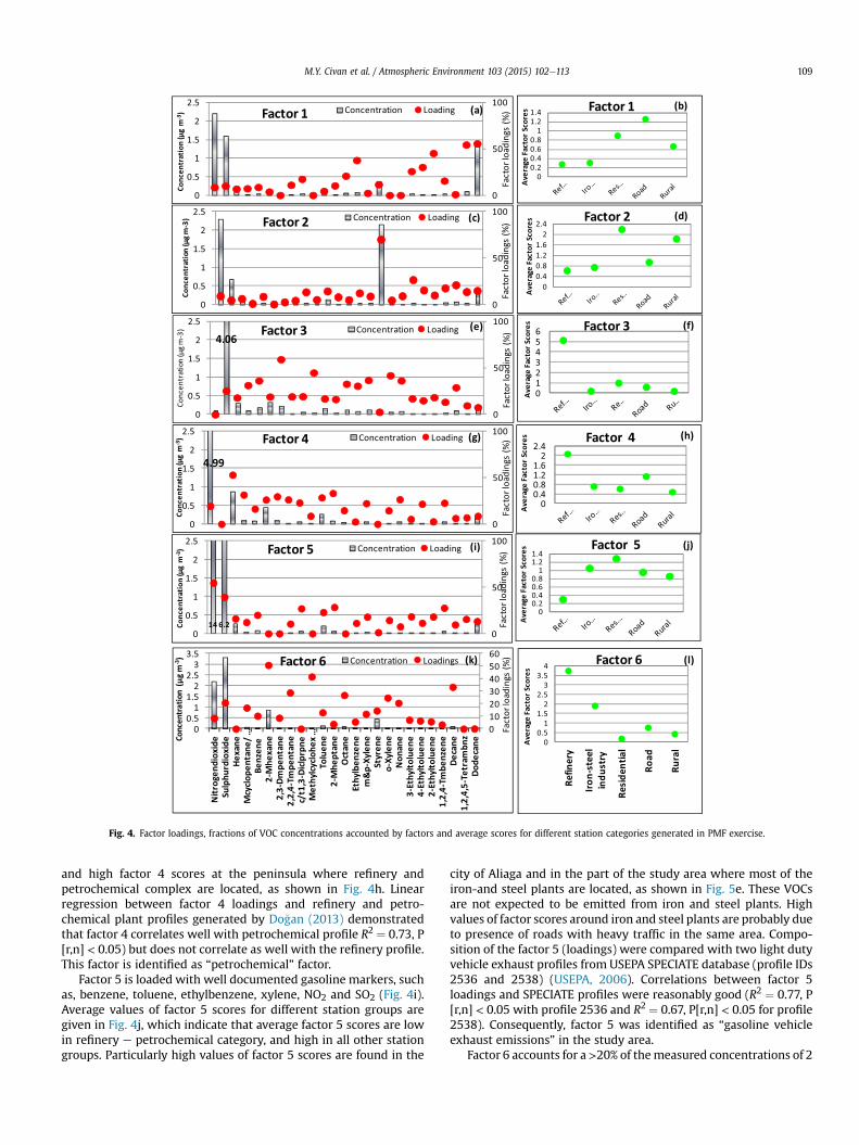
Fig. 4. Factor loadings, fractions of VOC concentrations accounted by factors and average scores for different station categories generated in PMF exercise.

M.Y. Civan et al. / Atmospheric Environment 103 (2015) 102e113 109

and high factor 4 scores at the peninsula where refinery andpetrochemical complex are located, as shown in Fig. 4h. Linearregression between factor 4 loadings and refinery and petro-chemical plant profiles generated by Do�gan (2013) demonstratedthat factor 4 correlates well with petrochemical profile R2 ¼ 0.73, P[r,n] < 0.05) but does not correlate as well with the refinery profile.This factor is identified as “petrochemical” factor.

Factor 5 is loaded with well documented gasoline markers, suchas, benzene, toluene, ethylbenzene, xylene, NO2 and SO2 (Fig. 4i).Average values of factor 5 scores for different station groups aregiven in Fig. 4j, which indicate that average factor 5 scores are lowin refinery e petrochemical category, and high in all other stationgroups. Particularly high values of factor 5 scores are found in the

city of Aliaga and in the part of the study area where most of theiron-and steel plants are located, as shown in Fig. 5e. These VOCsare not expected to be emitted from iron and steel plants. Highvalues of factor scores around iron and steel plants are probably dueto presence of roads with heavy traffic in the same area. Compo-sition of the factor 5 (loadings) were compared with two light dutyvehicle exhaust profiles from USEPA SPECIATE database (profile IDs2536 and 2538) (USEPA, 2006). Correlations between factor 5loadings and SPECIATE profiles were reasonably good (R2 ¼ 0.77, P[r,n] < 0.05 with profile 2536 and R2 ¼ 0.67, P[r,n] < 0.05 for profile2538). Consequently, factor 5 was identified as “gasoline vehicleexhaust emissions” in the study area.

Factor 6 accounts for a>20% of themeasured concentrations of 2

Fig. 5. Spatial distributions of PMF factor scores of (a) Factor 1, (b) Factor 2, (c) Factor 3, (d) Factor 4, (e) Factor 5, (f) Factor 6.

M.Y. Civan et al. / Atmospheric Environment 103 (2015) 102e113110

methylhexane, 2,2,4-threemethylpentane, methylcyclohexane, n-octane, o-xylene, n-nonane, and n-decane (Fig. 4k). It is difficult toassign a specific source for factor 6, by looking to these VOCs,because they are associated with a variety of sources includingvehicle exhaust (Liu et al., 2008), various domestic activities (Guoet al., 2004a), gasoline evaporation (Yamada, 2013), solvent evap-oration (Watson et al., 2001), surface coatings (Afshari, 1999), anddiesel exhaust (Srivastava et al., 2005). Although VOCs included infactor 6 are not ideal source tracers, their spatial distributionsshown in Figs. 4l and 5f provide information on potential sources ofthis factor. Average factor 6 scores were significantly higher inPetkim- Tupras category and iron and steel category, but low inroad, residential, and rural categories. Similarly, distribution mapfor factor 6, which is given in Fig. 5f depict high scores in both of theindustrial zones, where petrochemical plants, refinery, and iron e

steel industries are located. Furthermore factor 6 profile showedstatistically significant correlation (within 95% confidence level)with the refinery profile (Do�gan, 2013) but not with the petro-chemical profile. Therefore, this factor was attributed to emissionsoriginated from “petroleum refinery and iron-steel industries”.

Contributions of 6 factors extracted by the PMF model to themeasured VOC, NO2, and SO2 concentrations are illustrated in Fig. 7.PMF exercise revealed that light and heavy duty vehicle exhaustemissions were the highest contributors to VOCs levels in the area,accounting for 50% of the measured

P29VOCs concentration. In-

dustrial activities, particularly petrochemical industries and re-finery were the second highest contributors. These two industriesaccount for approximately 40% of the total VOC levels in the study

area. However, it should be pointed out that contribution of eachfactor to measured VOC concentrations showed dramatic differ-ences depending on the receptor location. Although traffic emis-sions were the highest contributor on the average, contribution ofPetkim and Tupras were much higher than light and heavy dutytraffic emissions in the sampling points located that are in the vi-cinity of these facilities. Strong variability of VOCs concentrationsaround industries is expected and documented in the literature(Parra et al., 2009; Civan et al., 2011), which is due to strong spatialvariations in source contributions around industries. This high-lights the most important advantage of determining source con-tributions using spatially distributed passive sampling data overassessments based on data generated at few permanent stations.Source contributions determined from one or two permanent sta-tions would probably not be representative for the study areawhere VOCs concentrations and source contributions show suchstrong spatial variability. Iron and steel industries turned out to beinsignificant VOCs sources as expected and emissions from do-mestic activities in villages were important only in their very closeproximity.

3.5. Lifetime carcinogenic risk estimation for benzene

A life-time cancer risk assessment was conducted for benzenebased on measured concentrations and data obtained from twoquestionnaires. One of the questionnaires was to generate time-eactivity data, and the second one to generate demograph-icepersonal data for people living at the Aliaga region. Details of

Fig. 6. Comparison of factor 3 profiles with profiles generated for a) Petkim and b)Tupras.

Fig. 7. Pie chart illustrating the contributions of 6 factors isolated by the model to receptor VOCs, NO2, and SO2 levels averaged for the sampling periods.

Fig. 8. Statistics, frequency and fitted distributions of cancer risk for benzene.

M.Y. Civan et al. / Atmospheric Environment 103 (2015) 102e113 111

these questioners are given in SI. Statistical evaluation of ques-tionnaire data showed that people living in the study area spend79% of their time within buildings for purposes, such as, living,working, resting and studying. This percentage is fairly similar withthe corresponding values reported by Guo et al. (2004b) andDodson et al. (2007) for people living in urban locations in HongKong and in sub-urban/urban locations in Boston, US, respectively.The participants naturally ventilated their indoor environment byopening the windows for 176 min/day, on average.

The lifetime cancer risk for benzene was estimated using MonteCarlo simulationmethod. Probability distributions of cancer risk for

benzene are given in Fig. 8. Mean, median, standard deviation ofthe distribution and the 95th percentile level are marked on thegraph.

The mean and median carcinogenic risks were 12.9 and 3.7 perone million population. These risks can be compared with USEPAbenchmark value of 1 per one million population. The differencebetween median and mean estimates pointed out the distributionof the carcinogenic risks was skewed (Zhou et al., 2011), which isprobably due to lognormal distribution of benzene concentration.The estimated mean carcinogenic risk levels are within the range ofthose calculated based on ambient measurements in Bejing, China(Zhang et al., 2012), in Seattle, USA (Wu et al., 2009), and in Port-land, USA (Tam and Neuman, 2004) which were reported as 15.3,8.8, and 41.9 per one million, respectively. It should be noted that,like benzene concentration, carcinogenic risk due to benzeneinhalation also showed large spatial differences between samplingpoints. It was significantly higher in the regions close to Petkim and

Tupras, but lower than calculated average risk in stations far fromindustries and roads. The PMF modeling results demonstrated that68% of benzene concentrations in the study area is due to emissionsfrom Petkim and Tupras, suggesting that at least half of the cancerrisk due to inhalation of benzene can be attributed to these twoplants.

4. Summary and conclusion

Spatial and temporal variations of concentrations of 32 VOCs,NO2, SO2 and O3 were determined at Aliaga, Turkey, which is a

M.Y. Civan et al. / Atmospheric Environment 103 (2015) 102e113112

densely populated industrial zone on the Aegean cost of Turkey,using passive samplers. Fifty-five passive sampling tubes wereplaced in approximately 30 km � 30 km study area. Distributionmaps ofmeasured compoundswerepreparedby interpolatingVOCsconcentrations at each sampling station using a GIS software. Highconcentrations of SO2 and most of the VOC were observed in theindustrial zone where petrochemical complex and the refinery arelocated. Concentrations of NO2 and some of the BTEX compoundswere also high around major roads. Ozone concentrations were thehighest at rural stations that are not under direct influence of anysource. This is attributed to destruction of O3 by NO in places whereNO concentration is high (also known as NO distillation).

Concentrations of most of the VOCs were high during winterseason due to lower mixing height. However, this observation wasnot true for all VOCs. Compounds that have evaporative sources andthose of which generation depends on solar flux (like O3) havehigher concentrations in summer season, or comparable concen-trations in both seasons.

The PMF was run after averaging data from five campaigns ateach station. Six factors that were associated with emissions fromheavy duty vehicles (diesel emissions), emissions from domesticactivities in settlement areas, combined emissions from Tupras andPetkim, emissions from Petkim, gasoline exhaust and emissionsfrom Petkim and iron and steel plants, were extracted by themodel.Among these, traffic emissions (light and heavy duty vehicles) werethe largest contributor to the measured VOC concentrations, ac-counting for approximately 50% of the total VOCs concentrations.Tupras and Petkim accounted for approximately 40% of

P29VOCs.

Remaining 10% is accounted for by factor 2, representing domesticactivities in towns and villages in the Aliaga region.

Distribution of factor scores suggested that source contributionsare highly variable, depending on the distance between the re-ceptor site and point sources. Consequently, although contributionof traffic to the measured VOCs concentrations were higher thancombined contributions of Petkim and Tupras on the average,contributions of these facilities were dominating in the peninsulawhere they are located. We believe that this is an importantadvantage of determining source contributions with a spatiallydistributed data, because sources and source contributions calcu-lated with data generated at one or two permanent stations doesnot represent the whole area. More control measures should bedeveloped to mitigate the VOCs and inorganic pollutants resultingfrom these two clusters of sources, namely Petkim and Tupras.

Potential cancer risk at Aliaga region, due to inhalation of ben-zene was calculated using a probabilistic approach, based on theassumption of lifetime exposure to benzene. Hence calculated riskwas probably to be underestimated mainly as only limited numberof species was monitored and there were no indoor measurementsthat should be included in data set. The mean and median carci-nogenic risks of benzene were 12.9 and 3.7 per one million popu-lation. Based on the source apportionment results thepetrochemical complex and refinery found to be largest contribu-tors (67%) to the benzene concentration in the region, followed byvehicular exhaust (27%). Despite a possible underestimation, theestimated risks still exceeded the acceptable level, suggesting thatthe pollutants with health hazards in this region are worth furtherinvestigation. The source apportionment and estimated lifetimecancer risk results presented in the paper can provide the guidancefor future health riskmanagers to design the risk reduction strategymore effectively.

Acknowledgement

This study was funded by the TÜB_ITAK through the project104Y276. We would also like to thank to Aliaga Municipality and

Izmir Metropolitan Municipalities, particularly Türkan Güngelenand Murat Gel from Aliaga Municipality for their valuable logisticsupport during sampling campaigns.

Appendix A. Supplementary data

Supplementary data related to this article can be found at http://dx.doi.org/10.1016/j.atmosenv.2014.12.031.

References

Afshari, A., 1999. Determination of VOC Emissions from Surface Coatings by Envi-ronmental Test Chamber Measurements. Doktorsavhandlingar Vid ChalmersTekniska Hogskola, pp. 1e152.

Atkinson, R., 2000. Atmospheric chemistry of VOCs and NOx. Atmos. Environ. 34,2063e2101.

ATSDR, 2014. Toxicology Information Sheets. Retrieved January 1, 2009, from theAgency for Toxic Substances and Disease Registry Web site. http://www.atsdr.cdc.gov/ (accessed May, 2014).

Badol, C., Locoge, N., Galloo, J.C., 2008. Using a source-receptor approach to char-acterise VOC behaviour in a French urban area influenced by industrial emis-sions: part II: source contribution assessment using the Chemical Mass Balance(CMB) model. Sci. Total Environ. 389, 429e440.

Baltrenas, P., Baltrenaite, E., Sereviciene, V., Pereira, P., 2011. Atmospheric BTEXconcentrations in the vicinity of the crude oil refinery of the Baltic region.Environ. Monit. Asses 182, 115e127.

Belis, C.A., Karagulian, F., Larsen, B.R., Hopke, P.K., 2013. Critical review and meta-analysis of ambient particulate matter source apportionment using receptormodels in Europe. Atmos. Environ. 69, 94e108.

Borbon, A., Locoge, N., Veillerot, M., Gallo, J.C., Guilermo, R., 2002. Characterizationof NMHCs in a French urban atmosphere: overview of the main sources. Sci.Total. Environ. 292, 177e191.

Cai, C., Geng, F., Tie, X., Yu, Q., An, J., 2010. Characteristics and source apportionmentof VOCs measured in Shanghai, China, Atmos. Environ 44, 5005e5014.

Cetin, E., Odabasi, M., Seyfioglu, R., 2003. Ambient volatile organic compound (VOC)concentrations around a petrochemical complex and a petroleum refinery. Sci.Total Environ. 312103e312112.

Chou, C.C.K., Lee, C.T., Chen, W.N., Chang, S.Y., Chen, T.K., Lin, C.Y., Chen, J.P., 2007.Lidar observations of the diurnal variations in the depth of urban mixing layer:a case study on the air quality deterioration in Taipei. Taiwan. Sci. Total. Environ.374, 156e166.

Civan, M.Y., Yorulmaz, S., Tuncel, G., 2012. Improvement of uptake rate equationsdepending on meteorological conditions for volatile organic compounds.Talanta 99, 720e729.

Civan, M.Y., Kuntasal, O.O., Tuncel, G., 2011. Source apportionment of ambientvolatile organic compounds in Bursa, a heavily industrialized city in turkey.Environ. Forensics 12 (4), 357e370.

Dodson, R.E., Houseman, E.A., Levy, J.I., Spengler, J.D., Shine, J.P., Bennett, D.H., 2007.Measured and modeled personal exposures to and risks from volatile organiccompounds. Environ. Sci. Technol. 41, 8498e8505.

Do�gan, G., 2013. Temporal Variation of Atmospheric Concentrations of SpeciatedVOCs at the Alia�ga Region (PhD. Thesis). Middle East Technical University,Ankara, Turkey.

EN 13528-1&2, 2002. Ambient Air Quality e Diffusive Samplers for the Determi-nation of Concentrations of Gases and Vapours e Requirements and TestMethods. Part 1: General Requirements, Part 2: Specific Requirements and TestMethods.

Fuzzi, S., Andreae, M.O., Huebert, B.J., Kulmala, M., Bond, T.C., et al., 2006. Criticalassessment of the current state of scientific knowledge, terminology, andresearch needs concerning the role of organic aerosols in the atmosphere,climate, and global change. Atmos. Chem. Phys. 6, 2017e2038.

Gorecki, T., Namiesnik, J., 2002. Passive sampling. Trends Anal. Chem. 21, 276e290.Goyal, S.K., Rao, C.C.V., 2007. Assessment of atmospheric assimilation potential for

industrial development in an urban environment: Kochi (India). Sci. Total En-viron. 376, 27e39.

Guo, H., Wang, T., Louie, P.K.K., 2004a. Source apportionment non-hydrocarbons inHong Kong: Application of a principal component analysis/absolute principalcomponent analysis/absolute principal component scores (PCA/APCS) receptormodel. Environ. Pollut. 129, 489e498.

Guo, H., Lee, S.C., Chan, L.Y., Li, W.M., 2004b. Risk assessment of exposure tovolatile organic compounds in different indoor environments. Environ. Res.94, 57e66.

Henschel, D.B., Fortmann, R.C., Roache, N.F., 2001. Potential for reducing indoorstyrene exposure from copied paper through use of low-emitting toners. J. Air &Waste Manage. Assoc. 53, 708e717.

Hoque, R.R., Khillare, P.S., Agarwal, T., Shridhar, V., Balachandran, S., 2008. Spatialand temporal variation of BTEX in the urban atmosphere of Delhi, India. Sci.Total. Environ. 392, 30e40.

Kalabokas, P.D., Hatzaianestis, J., Bartzis, J.G., Papagiannakopoulos, P., 2001. Atmo-spheric concentrations of saturated and aromatic hydrocarbons around a Greekoil refinery. Atmos. Environ. 35, 2545e2555.

M.Y. Civan et al. / Atmospheric Environment 103 (2015) 102e113 113

Kuntasal, O., Kilavuz, S.A., Karman, D., Wang, D., Tuncel, G., 2013. C5eC12 volatileorganic compounds at roadside, residential, and background locations inAnkara, turkey: temporal and spatial variations and sources. J. Air WasteManage. Assoc. 6, 1148e1162.

Lan, C.H., Huang, Y.L., Ho, S.H., Peng, C.Y., 2014. Volatile organic compound identi-fication and characterization by PCA and mapping at a high-technology sciencepark. Environ. Pollut. 193, 156e164.

Li, N., Hopke, P.K., Kumar, P., Cliff, S.S., Zhao, Y., Navasca, C., 2013. Source appor-tionment of time- and size-resolved ambient particulate matter. Chemom.Intelligent Laboratory Syst. 129, 15e20.

Ling, Z.H., Guo, H., 2014. Contribution of VOC sources to photochemical ozoneformation and its control policy implication in Hong Kong. Environ. Sci. Policy38, 180e191.

Lithner, D., Damberg, J., Dave, G., Larsson, A., 2009. Leachates from plastic consumerproducts e screening for toxicity with Daphnia magna. Chemosphere 74,1195e1200.

Liu, P.W.G., Yao, Y.C., Tsai, J.H., Hsu, Y.C., Chang, L.P., Chang, K.H., 2008. Source im-pacts by volatile organic compounds in an industrial city of southern. Taiwan.Sci. Total. Environ. 398, 154e163.

Miller, R.R., Newhook, R., Poole, A., 1994. Styrene production, use, and humanexposure. Crit. Rev. Toxicol. 24, 1e10.

Paatero, P., Hopke, P.K., 2003. Discarding or downweighting high-noise variables infactor analytic models. Anal. Chim. Acta 490, 277e289.

Parra, M.A., Elustondo, D., Bermejo, R., Santamaria, J.M., 2009. Ambient air levels ofvolatile organic compounds (VOC) and nitrogen dioxide (NO2) in a medium sizecity in Northern Spain. Sci. Total. Environ. 407, 999e1009.

Polissar, A.V., Hopke, P.K., Poirot, R.L., 2001. Atmospheric aerosol over Vermont:chemical composition and sources. Environ. Sci. Technol. 35, 4604e4621.

Ras, M.R., Marce, R.M., Borrull, F., 2009. Characterization of ozone precursor volatileorganic compounds in urban atmospheres and around the petrochemical in-dustry in the Tarragona region. Sci. Total Environ. 407, 4312e4319.

Ras, M.R., Marce, R.M., Borrull, F., 2010. Volatile organic compounds in air at urbanand industrial areas in the Tarragona region by thermal desorption and gaschromatographyemass spectrometry. Environ. Monit. Assess. 161, 389e402.

Rinsky, R.A., Smith, A.B., Hornung, R., Filloon, T.G., Young, R.J., Okun, A.H.,Landrigan, P.J., 1987. Benzene and leukemia an epidemiologic risk assessment.New. Engl. J. Med. 316, 1044e1050.

Song, Y., Dai, W., Shao, M., Liu, Y., Lu, S., Kuster, W., Goldan, P., 2008. Comparison ofreceptor models for source apportionment of volatile organic compounds inBeijing, China. Environ. Pollut. 156, 174e183.

Srivastava, A., Sengupta, B., Dutta, S.A., 2005. Source apportionment of ambientVOCs in Delhi City. Sci. Total Environ. 343, 207e220.

Tam, B.N., Neumann, C.M., 2004. A human health assessment of hazardous airpollutants in Portland, OR. J. Environ. Manage. 73/2, 131e145.

USEPA, 1999. PCRAMMET User's Guide. EPA-454/B-96e001. US EnvironmentalProtection Agency Office of Air Quality Planning and Standards Emissions,Monitoring, and Analysis Division Research Triangle Park, NC 27711.

USEPA SPECIATE, 2006. Data-base, Version 4.0. http://www.epa.gov/ttn/chief/software/speciate/index.html.

USEPAIRIS, 2013. Integrated Risk Information System/Benzene. US EnvironmentalProtection Agency, Cincinnati, OH. http://www.epa.gov/iris/subst/0276.htm(accessed December 2013).

Wang, T., Ding, A.J., Gao, J., Wu, W.S., 2006. Strong ozone production in urbanplumes from Beijing, China. Geophys. Res. Lett. 33, L21806.

Watson, J.J., Chow, J.C., Fujita, E.M., 2001. Review of volatile organic compoundsource apportionment by chemical mass balance. Atmos. Environ. 35,1567e1584.

Wu, C., Wu, S., Cullen, A.C., Larson, T.V., Williamson, J., Liu, L.-J.S., 2009. Cancer riskassessment of selected hazardous air pollutants in Seattle. Environ. Int. 35,516e522.

Xu, J., Ma, J.Z., Zhang, X.L., Xu, X.B., Xu, X.F., Lin, W.L., Wang, Y., Meng, W., Ma, Z.Q.,2011. Measurements of ozone and its precursors in Beijing during summertime:impact of urban plumes on ozone pollution in downwind rural areas. Atmos.Chem. Phys. Discuss. 11, 17337e17373.

Yamada, H., 2013. Contribution of evaporative emissions from gasoline vehiclestoward total VOC emissions in Japan. Sci. Total Environ. 449, 143e149.

Yang, F., Tan, J., Zhao, Q., Du, Z., He, K., Ma, Y., Duan, F., Chen, G., Zhao, Q., 2011.Characteristics of PM2.5 speciation in representative megacities and acrossChina. Atmos. Chem. Phys. 11, 5207e5219.

Yoo, H.J., Kim, J., Yi, S.M., Zoh, K.D., 2011. Analysis of black carbon, particulate matter,and gaseous pollutants in an industrial area in Korea. Atmos. Environ. 45,7698e7704.

Yurdakul, S., 2014. Temporal Variation of Volatile Organic Compound Concentra-tions in Bursa Atmosphere (PhD. Thesis). Middle East Technical University,Ankara, Turkey.

Yurdakul, S., Civan, M., Tuncel, G., 2013. Volatile organic compounds in suburbanAnkara atmosphere, Turkey: sources and variability. Atmos. Res. 120/121,298e311.

Zhang, Y., Mu, Y., Liu, J., Mellouki, A., 2012. Levels, sources and health risks of car-bonyls and BTEX in the ambient air of Beijing, China. J. Environ. Sci. 24,124e130.

Zhou, J., You, Y., Bai, Z., Hu, Y., Zhang, J., Zhang, N., 2011. Health risk assessment ofpersonal inhalation exposure to volatile organic compounds in Tianjin, China.Sci. Total Environ. 409, 452e459.