Sources, Pattern, and Health Impacts of PM2.5 inthe Central Region of Bangladesh using PMF, SOM,and Machine Learning TechniquesMd Shareful Hassan  ( shareful@gmx.com )

Jahangirnagar University https://orcid.org/0000-0003-4668-2951Mohammad Amir Hossain Bhuiyan 

Jahangirnagar UniversityS M Saify Iqbal 

Dhaka University: University of DhakaMuhammad Tauhidur Rahman 

King Fahd University of Petroleum & Minerals

Research Article

Keywords: PM2.5, ARI, PMF, SOM, Machine learning, Bangladesh

Posted Date: July 1st, 2022

DOI: https://doi.org/10.21203/rs.3.rs-1810022/v1

License: This work is licensed under a Creative Commons Attribution 4.0 International License.  Read Full License

1

Sources, Pattern, and Health Impacts of PM2.5 in the Central Region of Bangladesh 1

using PMF, SOM, and Machine Learning Techniques 2

3

Md. Shareful Hassan1*, Mohammad Amir Hossain Bhuiyan1, S M Saify Iqbal2, Muhammad Tauhidur Rahman3 4 5

1Department of Environmental Sciences, Jahangirnagar University, Dhaka, 1342, Bangladesh 62International Centre for Climate Change and Development (ICCCAD), Bangladesh 7

3Department of City and Regional Planning, King Fahd University of Petroleum and Minerals 8

KFUPM Box 5053, Dhahran – 31261, Kingdom of Saudi Arabia 9 10

11

12 13

14

*Corresponding author: Md. Shareful Hassan 15

Mailing address: Ph.D. Student, Environmental Science, Jahangirnagar University, Dhaka, Bangladesh 16

Email: shareful@gmx.com https://orcid.org/0000-0003-4668-295117

18

19

20

Abstract 21

The Particulate Matter 2.5 (PM2.5) is one of the major environmental and public health threats in Bangladesh. It 22

is important to explore the relationship between PM2.5, and other variables to mitigate its adverse health impacts. 23

This study aims to understand the sources, patterns, and health impacts of PM2.5 in five central districts of 24

Bangladesh using fourteen variables. These variables have been analyzed by PMF, SOM, Machine Learning, and 25

Multi-regression analysis. This paper has found that PM2.5 is correlated positively with NO (0.55), BC (0.45), CH4 26

(0.38), and NOx (0.22), while correlated negatively with Rainfall (-0.10), CO (-0.33), and SO2 (-0.24). In PMF 27

modeling, the R2 values of settlement density (1.00), SO2 (0.99), DEM (0.94), Rainfall (0.77), NO (0.74) and 28

Brickfield (0.66) have found as the most correlated variables. In this study, the dominant variables NO, CO, 29

Rainfall, O3, AOT, CH4, and BC are found in Factor 1; SO2, settlement density, and DEM are found in Factor 2; 30

and population density and brickfield are found in Factor 3. In SOM mapping, most of the variables are 31

concentrated in the north-eastern, central, and south-eastern parts of the study area. The prediction of PM2.5 using 32

machine learning is significant, showing reasonable R2 for Random Forest (0.85), Extreme gradient boosting 33

(0.81), and Stepwise Linear (0.76). The impact of PM2.5 on child ARI is significant (p=0.002, R2 =0.75); while 34

child mortality is not significant (p=0.268; R2 =0.55). These results will be useful for creating and implementing 35

local and regional PM2.5 mitigation plans. Concern institutions and academia may also use these outputs for 36

reducing health impacts, particularly child mortality and acute respiratory infections. 37

38

Keywords: PM2.5; ARI, PMF, SOM, Machine learning; Bangladesh. 39

40

1. Introduction 41

The Particulate Matter 2.5 (PM2.5) is a heterogeneous combination of suspended particles of various 42

chemical contents and sizes (Liang et al. 2013). The negative effects of PM2.5 are determined by its concentrations 43

in the atmosphere, which are influenced by a wide range of anthropogenic and natural sources (e.g., traffic 44

emissions, industrial processes, residential combustions, biogenic emissions), related factors (e.g., climate, 45

2

meteorological conditions, urbanization levels), and other events such as transportation and deposition of dust 46

particles (Ni et al. 2018; Adães and Pires 2019). Even at concentrations below ambient air quality standards, long-47

term exposures to PM2.5 particles has been linked to cardiovascular diseases, lung cancer, and both chronic and 48

acute respiratory diseases which ultimately lead to untimely death among children and adult population (Andersen 49

et al. 2012; Hoek et al. 2013; Raaschou-Nielsen et al. 2013; Beelen et al. 2014; Cesaroni et al. 2014). According 50

to many researchers, over 400,000 premature children die each year in EU countries as a result of PM2.5 (Badyda 51

et al. 2017; Cho and Song 2017). The PM2.5 particulates can penetrate deep into the human respiratory system due 52

to its small sizes, especially when exposed for lengthy periods of time (Eeftens et al. 2012; Tallon et al. 2017). 53

In Bangladesh, the concentration of PM2.5 particles in air is currently 15.4 times above the World health 54

Organization (WHO) annual air quality guideline value (IQAIR 2022). Between 2002 and 2019, the average 55

annual PM2.5 concentration has increased by 42% in the urban areas of the country due to excessive emissions 56

from various types of poorly maintained automobiles (Begum 2016; Hassan 2022). Furthermore, (Begum and 57

Hopke 2018) highlighted that Dhaka and other major cities of Bangladesh had some of the highest PM2.5 58

concentrations among the global cities for many years. PM2.5 causes roughly 234,000 premature deaths each year, 59

accounting for 3.5 percent of global data. Due to the rising trends of the PM2.5, it has been identified as a major 60

public health hazard for the people of Bangladesh, especially in the urban and semi-urban areas (Rahman et al. 61

2019). The high PM2.5 standard threshold also has significant impacts on vulnerable demographic groups, 62

especially for pregnant women, children, and elderly (over the age of 60) residents (Miller and Xu 2018). 63

Due to the excessive environmental threat and public health hazards, the sources, patterns, and possible 64

health impacts should be investigated for mitigating and implementing policies to reduce PM2.5 concentrations at 65

Bangladesh’s local, regional, and national levels. Some researchers have tried to identify the possible sources and 66

patterns of PM2.5 using Positive Matrix Factorization (PMF) model, its spatial concentration using Self-organizing 67

Map (SOM), machine learning for prediction of PM2.5, and regression analysis for possible health impacts 68

(Chueinta et al. 2000; Naz et al. 2015; Kim et al. 2018; Joharestani et al. 2019; Ulavi and Shiva Nagendra 2019; 69

Doreswamy et al. 2020; Liu et al. 2020). 70

The PMF model has recently gained popularity among scientists as an appropriate factorization receptor 71

model for calculating the contributions and sources of pollutants in the environment (Tao et al. 2017; Chen et al. 72

2019b). When sources are not formally identified, the PMF model is highly recommended, although it necessitates 73

post-treatment source identification. Using PMF analysis, (Nava et al. 2020) identified traffic congestions, 74

biomass burnings, secondary sulfates, secondary nitrates, urban dust storms, Saharan dust particles, and marine 75

aerosols as the seven main sources of PM2.5 in the city of Florence, Italy. Secondary sulfate was found to be a 76

significant PM2.5 source on a regional scale. (Sharma et al. 2016) also used the PMF model to find secondary 77

aerosols (21.3%) as the leading source of PM2.5, followed by soil dusts (20.5%), vehicle emissions (19.7%), 78

biomass burnings (14.3%), fossil fuel combustions (13.7%), industrial emissions (6.2%), and sea salts (4.3%) in 79

the city of Delhi, India. (Kim et al. 2018) assessed the sources of several pollutants that contribute to ambient fine 80

particles (PM2.5) in Daebu Island, Korea using PMF model. Chemical speciation data was used in this work to 81

estimate and identify possible PM2.5 sources using the PMF model. (Srivastava et al. 2021) used PMF modelling 82

in urban and rural areas of Beijing, China. One of the major limitations of these studies using PMF models is that 83

they have used chemical-based analysis of PM2.5 with minimum sample points in small geographical areas. 84

3

For mapping the hotspots of the distribution of PM2.5 pollutions, SOM became quite common recently. 85

A few researchers have used this to map the spatial distribution and concentration of each pollutant. However, the 86

integration of SOM and PMF could be a new technique for allocating different pollution sources in Bangladesh 87

(Hossain Bhuiyan et al. 2021). (Susanna et al. 2017) described the source characterization of PM10 and PM2.5 mass 88

concentrations using SOM by taking samples from Sardar Patel Road, Chennai, India during the winter months 89

of January and February of 2008. Their findings revealed that PM2.5 mass concentrations were high in their study 90

area due to contributions from six different sources: earth crust/soils, fugitive dusts, marine aerosol/sea, secondary 91

aerosols, traffic pollutions, and industries. (Srivastava et al. 2021) conducted a study on exploring the 92

spatiotemporal interrelation of PM2.5 concentration in Northern Taiwan by SOM using temporal datasets.(Lin et 93

al. 2022) evaluated the link between PM2.5 concentration, Weather Information System (WIS), precursors, and 94

meteorological factors to investigate the secondary aerosols generation mechanism and trace the likely sources of 95

PM2.5 during severe pollution episodes using SOM. However, SOM has not been used intensively in PM2.5 source 96

mapping for large geographical areas. 97

Machine learning is one of the cutting-edge tools for predicting the latent relationship between dependent 98

and different independent variables in air pollution studies. (Tian et al. 2016) estimated PM2.5 from multi-source 99

data where they employed different machine learning models in the Pearl River Delta (PRD) in China, using 100

Random Forest (RF) and Gradient Boosting Regression Tree (GBRT). (Deters et al. 2017) employed a machine 101

learning approach to estimate PM2.5 concentrations from wind (speed and direction) and precipitation levels, based 102

on six years of meteorological and pollutant data. A machine learning approach was developed by (Chen et al. 103

2018) to estimate the PM2.5 concentrations across China using remote sensing, meteorological, and land use data. 104

(Zhang et al. 2015) assessed the effects of various factors on PM2.5 pollution by merging the Random Forest 105

model, Shapley Additive exPlanations (RF-SHAP), Partial Dependence Plot (RF-PDP), and Positive Matrix 106

Factorization (PMF). They have found that anthropogenic emissions and climatic conditions both contributed 107

roughly 67% (40.5 µg/m3) and 33% (19.7 µg/m3) of the fluctuation in PM2.5 concentrations. In all of above-108

mentioned literature on machine learning, most of the works have used a very few sets of data and information as 109

well as very small sample data. Studies utilizing a large combination of air pollutants, climatic, environmental, 110

and social data for predicting PM2.5 is lacking and should be further investigated. 111

Measuring the impact of public health due to PM2.5 is a complex issue, as many hidden determinants are 112

involved. Exposure to ambient PM2.5 is associated with child mortality and acute respiratory infection (ARI), 113

which are found in Nairobi, Kenya (Egondi et al. 2018). To predict the statistical relationship of PM2.5 with child 114

mortality and ARI, many researchers have used multiple-regression modeling using an array of different datasets 115

(Dominici et al. 2002; Naz et al. 2015; Sultana and Uddin 2019). However, integration and analyses of local 116

hospital-based data with diverse air pollutants, and other variables were not examined. 117

Based on the literature review, this paper found that the combined use of different sets of data such as air 118

pollutants, environmental, climatic, and social, to identify the sources, patterns, and health impacts of PM2.5 is 119

lacking, especially for urban areas of Bangladesh. Furthermore, using PMF for source identification, GIS analysis 120

for factor mapping, SOM for concentration mapping/clustering, and machine learning for prediction of PM2.5 121

concentrations using factorized data and health impact using multi-regression modeling will be unique for the 122

country as well. Therefore, considering this knowledge gap, the goal of this study is to (1) determine the key 123

4

sources of PM2.5, (2) identify the core concentrated areas of the sources, (3) predict the PM2.5 using factorized 124

data, and (4) investigate the impacts of child mortality and ARI due to PM2.5 and other air pollutants in five central 125

districts of Bangladesh. The results and ultimate outcomes of the study could be used by the government, 126

concerned ministries, UN bodies, domestic and international NGOs, civil societies, and environmental activists 127

for local and regional level mitigation planning and implementations as well as achieve the goal of Sustainable 128

Development Goal (SDG)-11 with indicators 11.6 and 11.6.2. 129

2. Methods and Materials 130

2.1 Study area 131

The study area is located in the Dhaka division of Bangladesh, covering its five major industrial districts (Dhaka, 132

Gazipur, Narayanganj, Narsingdi, and Munshiganj). With an area of 6,043 km2, the study area is home to over 20 133

million residents (Fig. 1). The area has a tropical wet and dry climate, with annual average rainfall ranging from 134

694 mm to 2,376 mm (highest in Narsingdi district and lowest in Munshiganj district). According to (Deters et al. 135

2017), the air and water in the districts are becoming increasingly polluted because of increasing population, 136

decreasing wetland and green spaces, rising multi-storied buildings, and growing commercial real estate 137

developments. The areas also experience higher levels of traffic congestion, unplanned migration, and unplanned 138

urban activities (Begum and Hopke 2019; Rahman et al. 2019; Iqbal et al. 2020). In addition, the study area also 139

houses industries of ready-made garments, textiles, pharmaceuticals, cements, brickfields, fertilizers, and 140

processing of raw material. All of these are the primary triggering factors for massive emissions of PM2.5. 141

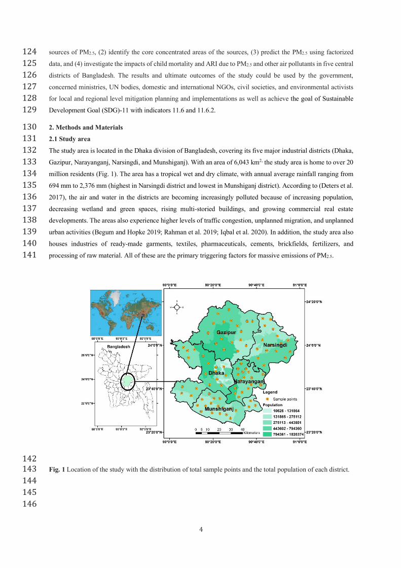
142

Fig. 1 Location of the study with the distribution of total sample points and the total population of each district. 143

144

145

146

5

2.2 Data sources and materials 147

For this study, numerous sources of data were gathered, processed, and analyzed. Some of these data 148

were obtained from the Bangladesh Bureau of Statistics (BBS), Bangladesh Department of Health (BDH), and 149

the Humanitarian Data Exchange Website. Data pertaining to air pollutants and their relevant parameters were 150

obtained from earth observing satellite sensors and were downloaded from various online sources. High-resolution 151

Google map was also used to digitize locations of brickfields. Table 1 summarizes the various parameters and 152

their data sources used in the study. 153

154

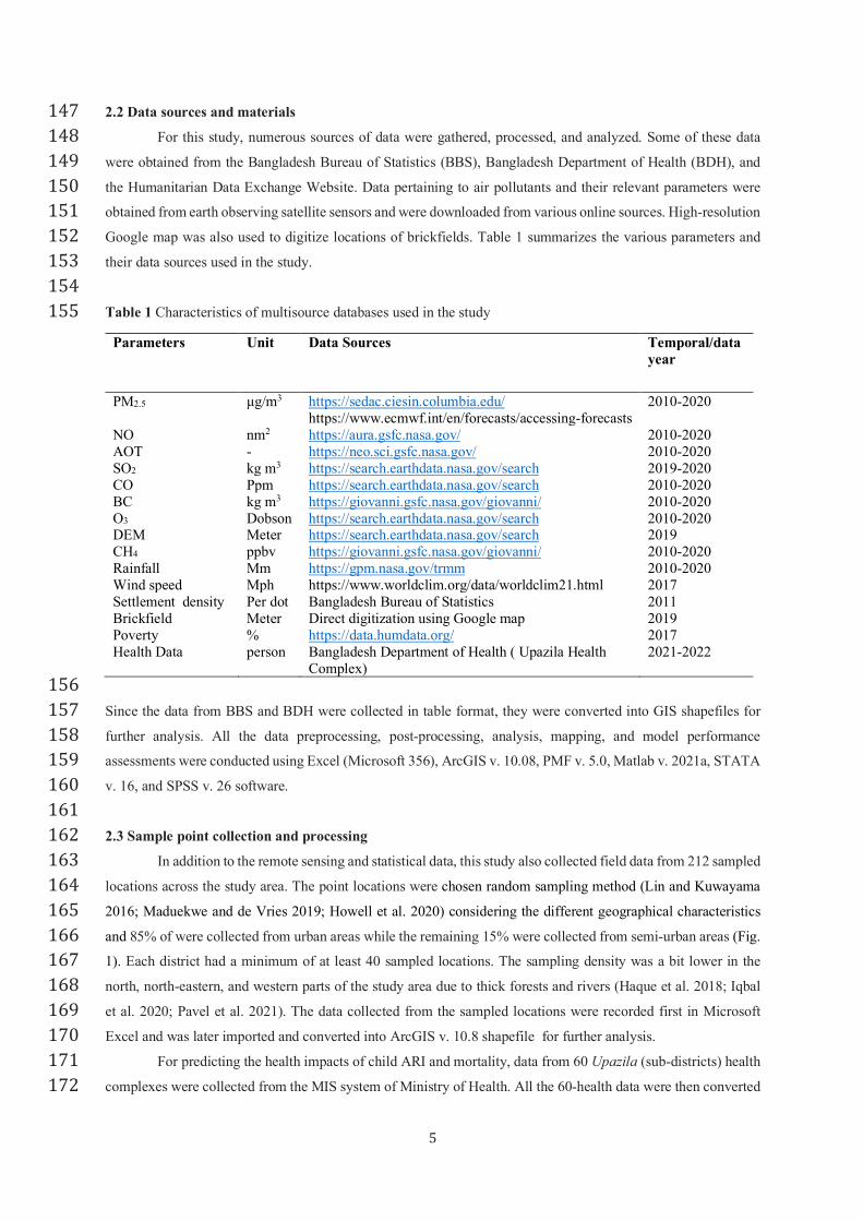
Table 1 Characteristics of multisource databases used in the study 155

Parameters

Unit Data Sources Temporal/data

year

PM2.5 µg/m3 https://sedac.ciesin.columbia.edu/

https://www.ecmwf.int/en/forecasts/accessing-forecasts

2010-2020

NO nm2 https://aura.gsfc.nasa.gov/ 2010-2020

AOT - https://neo.sci.gsfc.nasa.gov/ 2010-2020

SO2 kg m3 https://search.earthdata.nasa.gov/search 2019-2020

CO Ppm https://search.earthdata.nasa.gov/search 2010-2020

BC kg m3 https://giovanni.gsfc.nasa.gov/giovanni/ 2010-2020

O3 Dobson https://search.earthdata.nasa.gov/search 2010-2020 DEM Meter https://search.earthdata.nasa.gov/search 2019

CH4 ppbv https://giovanni.gsfc.nasa.gov/giovanni/ 2010-2020

Rainfall Mm https://gpm.nasa.gov/trmm 2010-2020

Wind speed Mph https://www.worldclim.org/data/worldclim21.html 2017

Settlement density Per dot Bangladesh Bureau of Statistics 2011

Brickfield Meter Direct digitization using Google map 2019

Poverty % https://data.humdata.org/ 2017

Health Data person Bangladesh Department of Health ( Upazila Health

Complex)

2021-2022

156

Since the data from BBS and BDH were collected in table format, they were converted into GIS shapefiles for 157

further analysis. All the data preprocessing, post-processing, analysis, mapping, and model performance 158

assessments were conducted using Excel (Microsoft 356), ArcGIS v. 10.08, PMF v. 5.0, Matlab v. 2021a, STATA 159

v. 16, and SPSS v. 26 software. 160

161

2.3 Sample point collection and processing 162

In addition to the remote sensing and statistical data, this study also collected field data from 212 sampled 163

locations across the study area. The point locations were chosen random sampling method (Lin and Kuwayama 164

2016; Maduekwe and de Vries 2019; Howell et al. 2020) considering the different geographical characteristics 165

and 85% of were collected from urban areas while the remaining 15% were collected from semi-urban areas (Fig. 166

1). Each district had a minimum of at least 40 sampled locations. The sampling density was a bit lower in the 167

north, north-eastern, and western parts of the study area due to thick forests and rivers (Haque et al. 2018; Iqbal 168

et al. 2020; Pavel et al. 2021). The data collected from the sampled locations were recorded first in Microsoft 169

Excel and was later imported and converted into ArcGIS v. 10.8 shapefile for further analysis. 170

For predicting the health impacts of child ARI and mortality, data from 60 Upazila (sub-districts) health 171

complexes were collected from the MIS system of Ministry of Health. All the 60-health data were then converted 172

6

into a GIS point shapefile, extracting the same locational values of all air pollutants and other variables. These 60 173

data points were used to run multi-regression analysis. 174

175

2.4 Positive Matrix Factorization (PMF) 176

Receptor models are mathematical methods for calculating the contribution of sources to samples 177

according to their composition or properties (USEPA 2014). Many studies have used receptor models recently, 178

and they have demonstrated their capacity to reliably identify potential ambient PM emission sources at a receptor 179

site (Waked et al. 2014). The PMF model is a multivariate receptor model that uses a weighted least square 180

approach to estimate the source profiles and their contributions (Paatero and Tapper 1994; Paatero 1997) and it is 181

extensively used in determining the air quality (Tan et al. 2014; Zhang et al. 2015). In this study, PMF (v. 5.0) 182

was used to quantify the contribution of various emission sources to PM2.5 (USEPA 2014). The model requires 183

two input files: one for the ‘species' measured concentrations and another for the ‘estimated uncertainty’ of the 184

concentrations (Sharma et al. 2016). Based on the PMF user guide, the equation below is used to identify the 185

number of factors p, species profile f, and factor to contribution g (USEPA 2014): 186

187

𝑥"# =%  '()* 𝑔"(𝑓(# + 𝑒"# 188

Where i and j are the number of samples and chemical species, and ej is the residual of individual sample/species. 189

The equation below is used for factor contribution and profiles. 190

191

𝑄 =% 0")* % 1

#)* 2𝑥"# − ∑  '()* 𝑔"(𝑓(#𝑢"# 67 192

Where Q is a critical factor, showing Q(true) and Q(robust). 193

Two input files, species concentration, and sample uncertainty are needed to run a PMF model. This study used 194

the following uncertainty equations (USEPA 2014): 195

𝑈𝑛𝑐 = 56 ×𝑀𝐷𝐿 196

Unc = A( Error Fraction × concentration )7 + (0.5 ×𝑀𝐷𝐿)7 197

Where Unc is the concentration of each sample, MDL is the sample-specific method limitation, and error fraction 198

is the percentage of measurement uncertainty. 199

200

2.5 Interpolation of point data 201

This paper used the point interpolation method to perform GIS mapping for all factors and visualize their 202

spatial concentration in the study area. The Inverse distance weighted (IDW) interpolation method was selected, 203

due to the near distances of each data point (Yu et al. 2019), to estimate the unknown values of new points 204

surrounding the nearest known points in the study area. This is a very crucial point interpolation method used in 205

many point source identification and public health data analyses (Feng et al. 2015; Hu et al. 2017; Huang et al. 206

2017; Iqbal et al. 2020). In this paper, factor 1 to 5 data was interpolated using ArcGIS v. 10.08 software. The 207

calculation of IDW is in the equation below: 208

209

Eq 01

Eq 02

Eq 03

Eq 04

Eq 05

7

𝑧# = ∑  G HGIGJ∑  G KILGJ 210

Where zi is the value of a known data point, dij is the distance of a known point, 𝑧# is the value at the unknown 211

point. 212

213

2.6 Self-Organizing Map (SOM) 214

The SOM is thought to be a suitable artificial intelligence tool for extracting features because the input 215

data is considered as a continuum rather than depending on correlation and cluster analysis (Liu et al. 2006). The 216

SOM has been widely utilized for data downscaling and visualization in different areas (Kohonen 1982). 217

Combining SOM with cluster analysis can help characterize various groupings of items that can logically be 218

classified as characteristics (Nakagawa et al. 2020). Because SOM is stronger at classifying and recognizing 219

patterns in elements, combining it with PMF could help SOM's findings to more accurately allocate contributions 220

from various sources (Pearce et al. 2014; Dyson 2015; Katurji et al. 2015; Stauffer et al. 2016; Jiang et al. 2017). 221

To imply such a concept, this paper used SOM to identify the pattern and concentration of each factorized data 222

by investigating all neurons and their neighborhood relations using Matlab v. 2021a. In SOM, a similar color 223

pattern shows a positive relationship while heterogeneous color shows a negative relationship, by clustering all 224

data. In addition to this, a SOM shows the spatial distribution of each variable in 2-dimensional space by following 225

the equation below: 226

227 ∥∥x −mP∥∥ = 𝑚𝑖𝑛{∥∥x − mT∥∥} 228

Where x is the input vector, m is the weight vector, and || || is the distance measure. 229

230

2.7 Machine learning in predicting PM2.5 231

Machine learning is the technique for creating computer algorithms that can emulate human intelligence. 232

It incorporates principles from several fields, including artificial intelligence, probability and statistics, computer 233

science, information theory, psychology, control theory, and philosophy (Michel 1997; Bishop 2017). Generally, 234

machine learning models are performed using numerous alternative algorithms to evaluate their effectiveness and 235

select the best prediction. Algorithms of machine learning include Extremely Randomized Trees Regression 236

(Extra Trees Regression), Random Tree, Stepwise linear, Linear Regression, Extreme Gradient Boosting 237

(XGBoost), Least Absolute Shrinkage, and Selection Operator (Minh et al. 2021). In this paper, three supervised 238

classifiers of machine learning (1) Random Tree (Joharestani et al. 2019) (2) Extreme gradient boosting (Ma et 239

al. 2020a), and (3) Stepwise Linear (Chen et al. 2019a) were used to predict the relationship between PM2.5 and 240

fourteen variables using Matlab v. 2021a. To run these three classifiers, this paper followed several steps (Minh 241

et al. 2021). The first step was to divide the pre-processing data into training and test data sets. Second, using the 242

training dataset, the machine learning model was trained using each algorithm. The test dataset was then placed 243

to evaluate the training efficiency of each method. The final stage was to assess each model's performance using 244

the assessment parameters. Lastly, the Mean Absolute Error (MAE), Root Mean Square Error (RMSE), Mean 245

Square Error (MSE), and Coefficient of Determination (R2) were used to evaluate the model performance of these 246

three classifiers. The key equations of these performance indexes are given below: 247

248

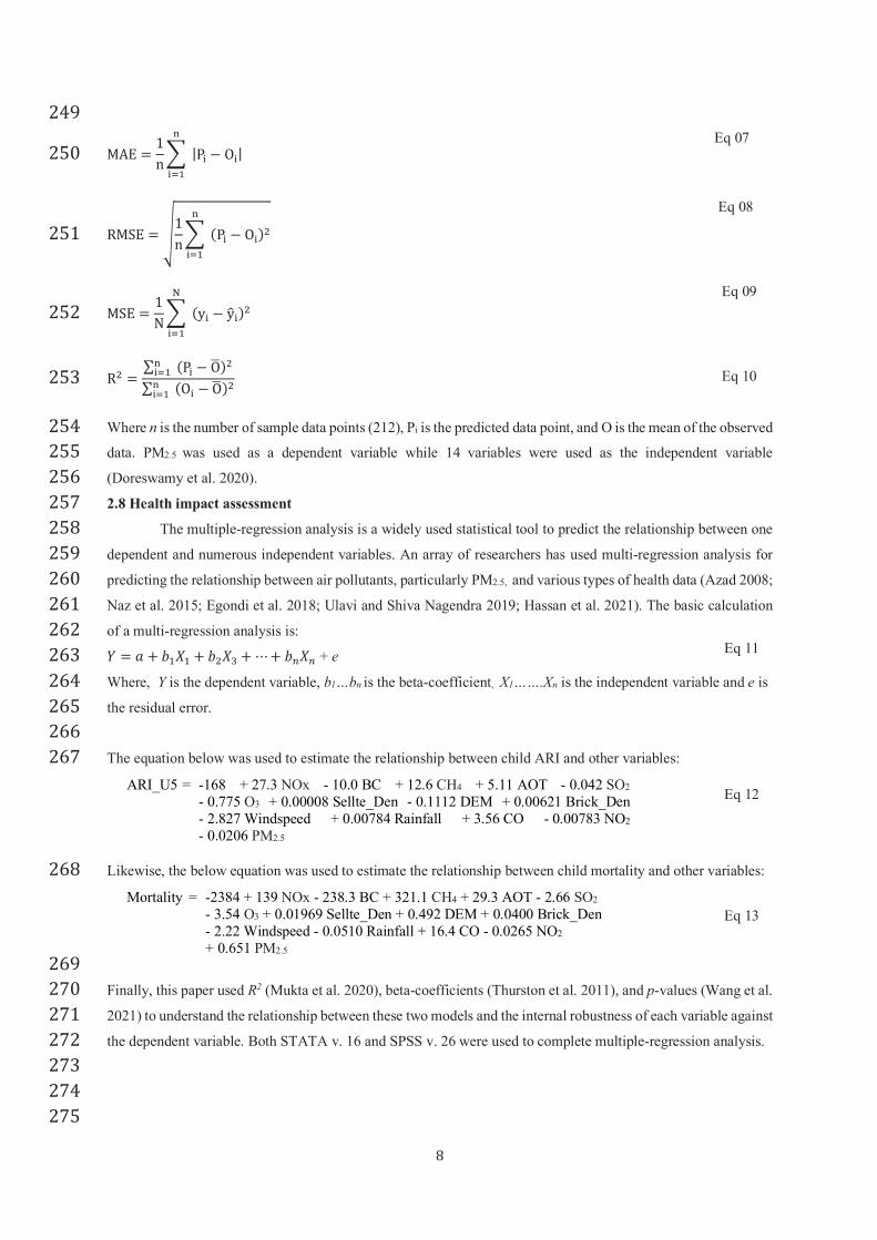
Eq 06

8

249

MAE = 1n%  [T)* |PT − OT| 250

RMSE = a1n% [T)* (PT − OT)7 251

MSE = 1N% cT)* (yT − yeT)7 252

R7 = ∑  [T)* (PT − Of)7∑  [T)* (OT −Of)7 253

Where n is the number of sample data points (212), Pi is the predicted data point, and O is the mean of the observed 254

data. PM2.5 was used as a dependent variable while 14 variables were used as the independent variable 255

(Doreswamy et al. 2020). 256

2.8 Health impact assessment 257

The multiple-regression analysis is a widely used statistical tool to predict the relationship between one 258

dependent and numerous independent variables. An array of researchers has used multi-regression analysis for 259

predicting the relationship between air pollutants, particularly PM2.5, and various types of health data (Azad 2008; 260

Naz et al. 2015; Egondi et al. 2018; Ulavi and Shiva Nagendra 2019; Hassan et al. 2021). The basic calculation 261

of a multi-regression analysis is: 262 𝑌 = 𝑎 + 𝑏*𝑋* + 𝑏7𝑋k +⋯+ 𝑏0𝑋0 + e 263

Where, Y is the dependent variable, b1…bn is the beta-coefficient, X1…….Xn is the independent variable and e is 264

the residual error. 265

266

The equation below was used to estimate the relationship between child ARI and other variables: 267

ARI_U5 = -168 + 27.3 NOx - 10.0 BC + 12.6 CH4 + 5.11 AOT - 0.042 SO2

- 0.775 O3 + 0.00008 Sellte_Den - 0.1112 DEM + 0.00621 Brick_Den

- 2.827 Windspeed + 0.00784 Rainfall + 3.56 CO - 0.00783 NO2

- 0.0206 PM2.5

Likewise, the below equation was used to estimate the relationship between child mortality and other variables: 268

Mortality = -2384 + 139 NOx - 238.3 BC + 321.1 CH4 + 29.3 AOT - 2.66 SO2

- 3.54 O3 + 0.01969 Sellte_Den + 0.492 DEM + 0.0400 Brick_Den

- 2.22 Windspeed - 0.0510 Rainfall + 16.4 CO - 0.0265 NO2

+ 0.651 PM2.5

269

Finally, this paper used R2 (Mukta et al. 2020), beta-coefficients (Thurston et al. 2011), and p-values (Wang et al. 270

2021) to understand the relationship between these two models and the internal robustness of each variable against 271

the dependent variable. Both STATA v. 16 and SPSS v. 26 were used to complete multiple-regression analysis. 272

273

274

275

Eq 07

Eq 08

Eq 09

Eq 10

Eq 11

Eq 12

Eq 13

9

3. Results and Discussion 276

3.1 Descriptive statistics of all sample points 277

The descriptive statistics of each variable are shown in Table 2. Data analysis highlighted that the mean 278

concentration of all the variables ranges from 0.55 to 82.11. Among all the variables, the mean concentration was 279

the highest for CO (82.11) followed by Poverty (73.59), PM2.5 (65.19), NO (56.63), Rainfall (27.46), and 280

Settlement density (23.52). The lowest mean concentration was for AOT (0.55). In addition, in comparison with 281

other variables, Standard Deviation was higher for Brickfield (51.99), Rainfall (44.11), No (12.91), and Settlement 282

(10.88), which indicated that these variables have a higher level of spatial variation compared to other variables. 283

Also, the Coefficient of variation is high in the brick field (2.17). 284

285

Table 2 descriptive statistics of all parameters used in this paper. 286

Mean Std. Deviation Coefficient of Variation

NOx 1.19 0.00 0.00

BC 0.67 0.01 0.02

CH4 6.33 0.03 0.00

AOT 0.55 0.04 0.08

SO2 1.02 0.37 0.36

O3 23.28 0.77 0.00

Settlement 23.52 10.88 0.46

DEM 10.02 3.56 0.35

Brickfield 23.67 51.99 2.17

Poverty 73.59 2.86 0.03

Wind Speed 2.10 0.20 0.09

Rainfall 27.46 44.11 0.16

CO 82.11 0.09 0.00

NO 56.63 12.91 0.22

PM2.5 65.19 1.26 1.58

287

3.2 Correlation analysis 288

Spearman’s Correlation method was applied among the fifteen variables ( including PM2.5) to know 289

which variables were correlated positively and negatively with each other (Fig. 2). From the data analysis, it was 290

observed that NO and CH4 (0.83), CO and DEM (0.58), and CH4 and BC (0.56) had strong positive relationships 291

(p>0.05). On the other hand, NO and CO (-0.80), CO and CH4 (-0.69), CO and Rainfall (-0.68), and Rainfall and 292

DEM (-0.82) showed a moderate to very strong negative relationships (p>0.05). Moreover, Brickfield was one of 293

the weaker variables with all other variables except for PM2.5 (0.25). PM2.5 was positively correlated with NO 294

(0.55), BC (0.45), CH4 (0.38) and NOx (0.22), while negatively correlated with Rainfall (-0.10), CO (-0.33), and 295

SO2 (-0.24). 296

297

10

298

Fig. 2 Results of Spearman’s Correlation of all variables, where *p < .05, **p < .01, ***p < .001 299

300

3.3 PMF process for source appointment 301

As state previously, to classify and quantity the key sources of PM2.5 in the study area and to determine 302

the major fingerprint of each pollutant, this study used PMF Model (version 5.0) using 19 variables (Fig. S1). 303

First, about 212 sample points were added to the model along with 212 uncertainty data (Table S1). Then, the 304

model was executed 20 times until the following conditions were met: having 1-5 factors, considering the base 305

random seed of 98, 0% extra modeling uncertainty, bootstraps value of 100, and minimum R2 value of 0.2. All the 306

input data were defined as “Strong” variables, except for APR, Pop density, LST, HCHO, and poverty. Five 307

variables (APR, population density, HCHO, LST, and water vapor) were excluded from this analysis as they were 308

not statistically significant. Finally, the standard model was selected when the Q values reached close to +1. As 309

an outcome of the PMF model, the coefficient of determination (R2) between the observed and predicted value of 310

each pollutant is shown in Fig. 3. 311

11

312

313

Fig. 3 Relationship between the observed and predicted of each pollutant generated from the PMF modeling. 314

315

The R2 values of settlement density (1.00), SO2 (0.99), DEM (0.94), Rainfall (0.77), NO (0.74) and Brickfield 316

density (0.66) were found to be the most correlated and significant variables in this model. Black Carbon, AOT, 317

Wind Speed, and CH4 had lower R2 values ranging from 0.26 to 0.38. 318

319

3.3.1 Factor profile analysis 320

In this study, the first factor was highly dominated by NO (70%) and Rainfall (60%). It suggests that 321

both traffic, diesel engine, and climatic factors are the responsible sources for PM2.5. Different emissions from 322

traffic and vehicles are being significantly contributed to about 2/3rd of air pollution in Dhaka and its surrounding 323

areas (Hassan et al. 2019). A study by (Pavel et al. 2021) showed that NO contributes ~74% to factor 1. (Begum 324

and Hopke 2019) suggested that rainfall and other metrological factors have a critical influence on PM2.5 in 325

Bangladesh. Moreover, about 50% of loading of CO, water vapor, O3, BC, and NOx were found as second 326

contributed sources in this factor 1 (Fig. 4). These gaseous substances have a substantial role as the major source 327

of PM2.5 (Zhang et al. 2013; Rahman et al. 2017; Samek et al. 2017). Like other particulate matter, BC emissions 328

mainly from the incomplete combustion of fossil fuels, biofuels, and biomass have long-term negative 329

implications for both public health and global climatic changes (Haque et al. 2018). In addition to factor 1, 330

unplanned urban development, uncovered construction materials, huge population, emissions from different 331

industries, less vegetation coverage, narrow road transportation systems, brick fields, and transboundary air flow 332

from, neighboring countries have all played major catalysts to increase PM2.5 in Dhaka and the surrounding 333

districts in the study area (Begum et al. 2009; Hasan et al. 2013; Rahman et al. 2017; Iqbal et al. 2020). 334

The second factor was depicted by SO2 (55%) and settlement density (54%). The main sources of 335

generating SO2 are mainly anthropogenic processes including motor vehicles, emissions from brick fields, 336

industries, and urbanization (Zhang et al. 2013; Mukta et al. 2020). (Huang et al. 2017) used a land use regression 337

model in China using three independent variables to predict the PM2.5, where SO2 explained the highest variance 338

(83%). (M.M. et al. 2018) mentioned that ready-made garment (RMG) factories in Bangladesh release huge 339

amounts of wastes, liquid particulates, and gaseous substances, which are the key components for increasing SO2 340

in major urban areas. The consumption level of liquefied petroleum gas (LPG) and electricity at the urban 341

household level is very common in Bangladesh. It is expected that about 36.5% of the total country has been 342

speculated to be urbanized (BBS 2020). The emissions from LPG and electricity have a significant outcome on 343

12

PM2.5 as well as overall air pollutions (Muindi et al. 2016; Fotheringham et al. 2019). In addition, the digital 344

elevation model (DEM) was loaded moderately by 50%, while settlement density was more than 50% (Fig. 4). 345

The third factor was dominated by population density with a loading of 60%, which was a high maker in 346

this group. Many researchers concluded that a higher density of urban population increases emissions from cars, 347

traffic patterns, slow travel speeds, compact roads, and unplanned urbanization, which are mainly the triggering 348

factors for PM2.5 (Chueinta et al. 2000; Han and Sun 2019; Nouri et al. 2021). As a result of migration from 349

climate changes across Bangladesh, more than 4.1 million people have been displaced and relocated to urban areas 350

(Khan et al. 2021). These populations are being created into huge urban slums and formed informal economic 351

activities for their daily lives and livelihoods. Slums and low-income settings have a significant role to enhance 352

PM2.5 due to their household fuel consumption, use of stoves, and poor ventilation systems (Gaita et al. 2014; 353

Muindi et al. 2016). In addition to factor 3, brickfield contributed about 30% of loading (Fig. 4). There are more 354

than 4,500 brick fields in and around the Dhaka division, which are mainly run by traditional coal and biomass 355

fuels (Haque et al. 2018). In turn, these brick fields are producing various gaseous and particulate matters in the 356

study area. 357

The fourth factor was characterized by settlement density (49%). This is one of the crucial urban 358

problems in Bangladesh. Increasing population, settlement, and manufacturing agglomeration for overall local 359

and regional economic development have fetched a signature of emitting pollution from diverse sources (Zhao et 360

al. 2021). Different urban landscape patterns like edge density (ED) and patch density (PD) are influenced by 361

PM2.5 in urban settings (Wu et al. 2015). As a second major source of this factor, brick field (Fig. 4) was dominated 362

by 30% loading in the north and central parts of the study area. (Al Nayeem et al. 2019) mentioned that about 363

92% of brick fields use fixed chimney kilns (FCKs), which emit dusts, fine coal, organic matters, and some 364

gaseous particles. Even the location of roadside brick fields increases the concentration of PM2.5 along with rapid 365

urbanization activities. 366

The fifth factor was dominated by brick field and SO2 (Fig. 4) with the loading of 60% and 10%. As a 367

major by-product of brickfield, SO2 pollutes the quality of air. About 7,500 brick fields across Bangladesh are 368

being operated illegally, violating the Environmental Conservation Rules (DoE 2022). Each year, more than 369

20,00,000 metric tons of raw fire wood and low-quality coals are burned in these brick fields by the traditional 370

brick-making processes, which are emitting SO2, CO2, and TSP (Ahmed and Hossain 2008). It is noted that 371

traditional, non-eco-friendly, and non-compliant brick kilns enhance PM2.5 and are susceptible to unhealthy 372

atmospheric conditions (Saha and Hosain 2016). (Thygerson et al. 2019) concluded that brick fields along with 373

population density and urban traffic have far exceeded the standard levels in Bhaktapur, Nepal. In turn, the emitted 374

gaseous and particulate matters have impacted public health, crops, vegetation, and land uses (Rahman 2022). 375

13

376

377

378

379

380

381

382

383

384

385

386

387

388

389

390

391

Fig. 4 Factor profile and source contribution from the PMF modeling. 392

393

3.3.2 GIS mapping of all factors and their spatial concentration 394

To understand the spatial distribution of each factor (Table S1), the inverse distance weighted (IDW) 395

interpolation method was used. The highest spatial concentration of factor 1 was found in the central to the 396

northern parts of the study area, covering central Dhaka and Gazipur districts (Fig. 5a). The mean concentration 397

of this factor was 1.00, the standard deviation was 0.49 with a 0.06 confidence interval (95%). Both areas have 398

been exposed to a high concentration level of emission due to huge traffic, construction works, the RMG sector, 399

and massive industrial activities. Moreover, unplanned urbanization activities, reduced vegetation areas, and 400

inadequate transportation systems have all created atmospheric pollutions, particularly PM2.5 (Hasan et al. 2020). 401

In Dhaka, the recent urbanization and various city development projects like elevated express, flyovers, new 402

buildings, an extension of the airport, shrinkage of water bodies, uncontrolled land development and landfills have 403

all caused heavily deteriorating air quality by releasing different gaseous and particulate matters (Nahar et al. 404

2021). On the other hand, Factor 2 was loaded in the central, south, and eastern parts of the study area, including 405

Dhaka, Munshiganj, and Narshingdi districts (Fig. 5b). The mean concentration of this factor was 0.99, the 406

standard deviation was 0.38 with a 0.52 confidence interval (95%). It is noted that most of the ready-made garment 407

factories, dyeing industries, and informal machine factories are located in both Munshiganj and Narshingdi 408

districts, which are producing vast amount of emissions (M.M. et al. 2018). Even more, enormous uncontrolled 409

brick fields have been installed and are operating in these areas (Haque et al. 2018; Rahman 2022). In Factor 3 410

(Fig. 5c), a pollution hotspot was found in central Dhaka and in the southern part of the Narayanganj districts, 411

with a mean concentration value of 1.00 and standard deviation of 3.28 with a 0.44 confidence interval (95%). 412

Several waterbodies have been flowing in these areas. Due to lower transportation costs for firewood, supply 413

bricks, cheaper labor costs, and the availability of quality clay, brick kilns were established in these areas (Hassan 414

et al. 2019). Factor 4 (Fig. 5d) was dominated in the northern part of Narshingdi and the western part of Dhaka 415

14

districts. The mean concentration of this factor was 0.99 and the standard deviation was 1.51 with a 0.20 416

confidence interval (95%). Many studies have found that both of these cities are releasing different gaseous and 417

particulate matters and are affecting the local public health, ecology, and ecosystems (Hasan et al. 2013; Al 418

Nayeem et al. 2019; Iqbal et al. 2020; Pavel et al. 2021) . In Factor 5, sporadic loading of a few variables was 419

found in few areas of Dhaka, Munshiganj, and Narayanganj districts (Fig. 5e). The mean concentration of this 420

factor was 0.99 with a standard deviation of 3.17 with a 0.43 confidence interval (95%). Factor 5 was not found 421

to be a major concern in identifying the key sources of PM2.5 in this study. 422

From this analysis, it is observed that Dhaka, Gazipur, Narayanganj, and Narshingdi are the prominent 423

areas for generating different sources of PM2.5 due to similar anthropogenic, natural, and development patterns. 424

While the results of this analysis are satisfactory considering the discussion and published literature, a major 425

limitation is not considering seasonal concentration levels. This study used average annual data from earth 426

observing satellite sensors. Perhaps, seasonal data may reveal a better understanding of possible sources. Further 427

investigation is needed to explore this variation. 428

429

Fig. 5 The spatial concentration mapping of all five factors from the PMF modeling, where factor 1 (5a), factor 2 430

(5b), factor 3 (5c), factor 4 (5d), and factor 5 (5e). 431

432

3.4 Concentration mapping using SOM 433

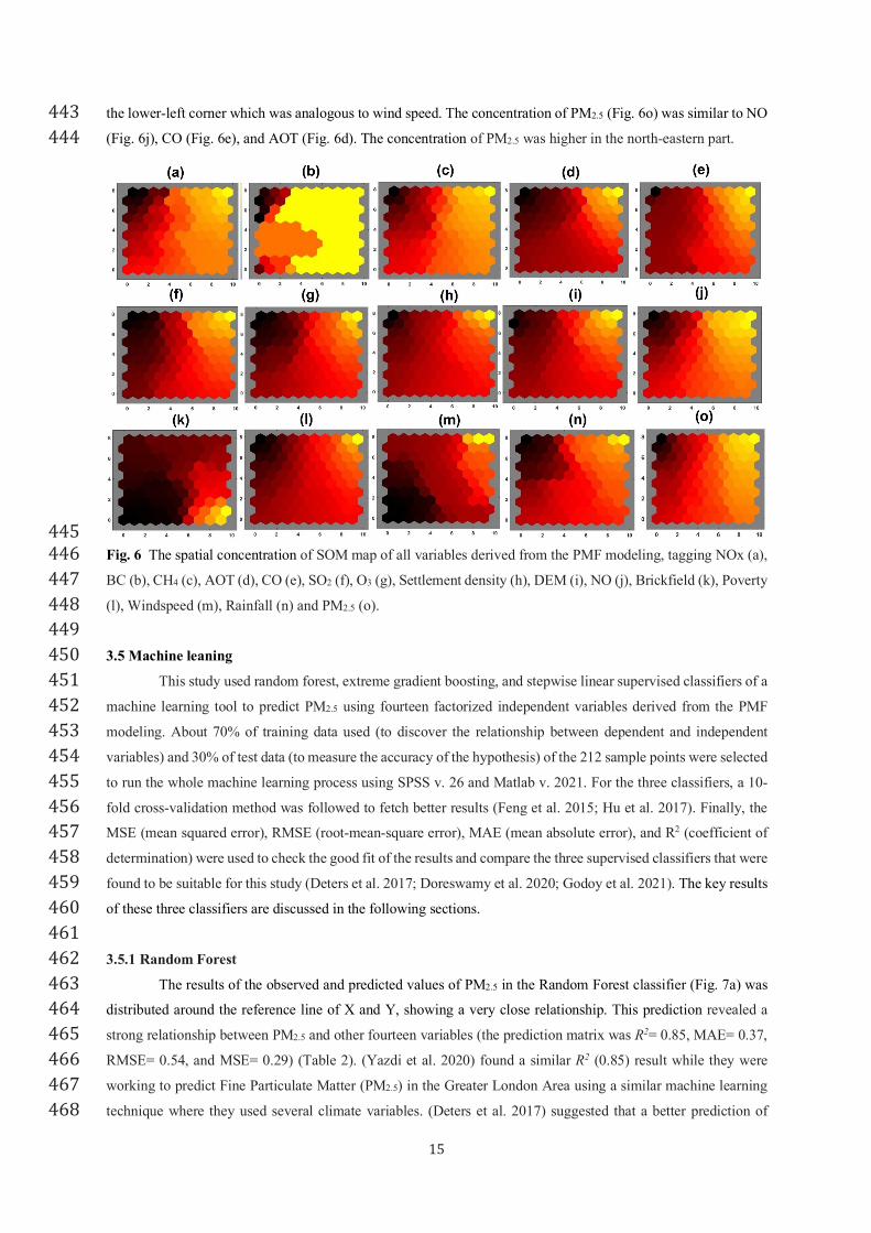
In Figure 06, the output of the component planes of the SOM analysis is shown in detail. Color-coded 434

SOM planes were created to highlight the concentration of the given variables for each SOM unit. The more 435

similar the properties of samples are, the smaller the hexagonal space is. A similar color indicates a positive 436

correlation between variables in a component plane, while dissimilar colors indicate negative correlations. 437

In most of the samples, the upper right corner of the map showed a higher concentration. No variable 438

was found to be highly concentrated in the left part. The variables O3 (Fig. 6g), Poverty (Fig. 6l), NO (Fig. 6j), 439

Settlement Density (Fig. 6g), CH4 (Fig. 6c), and DEM (Fig. 6i) showed a similar pattern of concentration which 440

indicated a common association and a positive correlation among these variables. For BC (Fig. 6b), most of the 441

portion of the component plane had high concentrations. In addition, the brick field had lower concentrations at 442

15

the lower-left corner which was analogous to wind speed. The concentration of PM2.5 (Fig. 6o) was similar to NO 443

(Fig. 6j), CO (Fig. 6e), and AOT (Fig. 6d). The concentration of PM2.5 was higher in the north-eastern part. 444

445

Fig. 6 The spatial concentration of SOM map of all variables derived from the PMF modeling, tagging NOx (a), 446

BC (b), CH4 (c), AOT (d), CO (e), SO2 (f), O3 (g), Settlement density (h), DEM (i), NO (j), Brickfield (k), Poverty 447

(l), Windspeed (m), Rainfall (n) and PM2.5 (o). 448

449

3.5 Machine leaning 450

This study used random forest, extreme gradient boosting, and stepwise linear supervised classifiers of a 451

machine learning tool to predict PM2.5 using fourteen factorized independent variables derived from the PMF 452

modeling. About 70% of training data used (to discover the relationship between dependent and independent 453

variables) and 30% of test data (to measure the accuracy of the hypothesis) of the 212 sample points were selected 454

to run the whole machine learning process using SPSS v. 26 and Matlab v. 2021. For the three classifiers, a 10-455

fold cross-validation method was followed to fetch better results (Feng et al. 2015; Hu et al. 2017). Finally, the 456

MSE (mean squared error), RMSE (root-mean-square error), MAE (mean absolute error), and R2 (coefficient of 457

determination) were used to check the good fit of the results and compare the three supervised classifiers that were 458

found to be suitable for this study (Deters et al. 2017; Doreswamy et al. 2020; Godoy et al. 2021). The key results 459

of these three classifiers are discussed in the following sections. 460

461

3.5.1 Random Forest 462

The results of the observed and predicted values of PM2.5 in the Random Forest classifier (Fig. 7a) was 463

distributed around the reference line of X and Y, showing a very close relationship. This prediction revealed a 464

strong relationship between PM2.5 and other fourteen variables (the prediction matrix was R2= 0.85, MAE= 0.37, 465

RMSE= 0.54, and MSE= 0.29) (Table 2). (Yazdi et al. 2020) found a similar R2 (0.85) result while they were 466

working to predict Fine Particulate Matter (PM2.5) in the Greater London Area using a similar machine learning 467

technique where they used several climate variables. (Deters et al. 2017) suggested that a better prediction of 468

16

PM2.5 derives when the climatic conditions are used (like strong wind or high levels of precipitation). This current 469

paper followed the same notion by adding some climatic variables (rainfall and wind speed). (Dai et al. 2021) 470

estimated the R2 (0.85) for the annual prediction of PM2.5 in the US, which is similar to this paper's result too. 471

472

3.5.2 Extreme gradient boosting 473

The relationships between observed and predicted values of PM2.5 using an extreme gradient boosting 474

classifier is shown in Fig. 7b. The relationships between PM2.5 and the independent variables were reasonably 475

strong (R2= 0.81, MAE= 0.32, RMSE= 0.51, and MSE= 0.26) (Table 3). Pan 2018 researched to predict the hourly 476

PM2.5 concentration in Tianjin city, China and found a strong R2 (0.95) between observed and predicted values. 477

The result found in this study was a bit lower since Pan (2018) used hourly predictions of PM2.5. (Dai et al. 2021) 478

used spatio-temporal feature selection to predict PM2.5 in the Fenwei plain, China. Their estimated R2 was about 479

0.87 with a higher RMSE (11.07). Interestingly, an R-value of –0.65 was found in the eastern Chinese city of 480

Shanghai. (Ma et al. 2020b) concluded this negative value was estimated because predicted PM2.5 and 481

meteorological factors were smaller than other pollutions used as independent variables. On the other hand, (Pan 482

2018) found a robust R2 (0.95) using the extreme gradient boosting classifier to PM2.5 concentration in Tianjin 483

city, China. 484

485

486

487

488

489

490

491

492

493

494

Fig. 7 Scatterplot of predicted and observed values of PM2.5. Figure 7a is the Random Forest, 7b is the Extreme 495

gradient boosting while 7c is the Stepwise linear. 496

497

Table 3 the key parameters derived from three classifiers to assess the prediction accuracy. 498

Classifier MSE RMSE MAE R2

Random forest 0.29 0.54 0.37 0.85

Extreme gradient boosting 0.26 0.51 0.32 0.81

Stepwise Linear 0.38 0.62 0.43 0.76

499

3.5.3 Stepwise Linear Classifier 500

The observed and predicted values of PM2.5 using a Stepwise linear classifier is shown in Fig. 7c. The 501

prediction matrix was for R2= 0.76, MAE= 0.43, RMSE= 0.62 and MSE= 0.38 (Table 3). This classifier showed 502

a slightly less performance accuracy than the other two classifiers used in this study. (Wu et al. 2015) studied how 503

urban landscape patterns affected PM2.5 in Beijing, China using stepwise linear modeling. They found a lower R2 504

17

(0.65) compared to the current study due to different urban landscapes associated with other variables like air 505

follow, traffic congestions, population density, etc. (Chen et al. 2019b) predicted the annual average of PM2.5 in 506

ESCAPE sites in Europe using 16 algorithms of machine learning with even lower R2 (0.61) due to the inclusion 507

of NO2. The R2 (0.70) was calculated by (Ulavi and Shiva Nagendra 2019) in Chennai, India. While they used 508

several meteorological variables, their coefficient of determination was the closest to the results obtained in this 509

study. 510

Long-term prediction of PM2.5 considering different variables with temporal sessional variations can be 511

a better management tool for local and regional level air pollution mitigation. This study has not used any temporal 512

sessional data. The inclusion of sessional and other data is suggested in its future study. 513

514

3.6 Health Impact analysis 515

The possible health impacts of mortality and ARI of children under the age of five due to different air 516

pollutants were estimated separately using multiple-regression analysis. 517

Table 4 highlights the relationship between child mortality and fourteen air pollutants. The results show 518

that the relationship was moderately statistically significant, with an R2 of 0.55. The significant P-values were in 519

BC, CH4, and settlement density at 0.01, 0.00, and 0.02, respectively with a 95% confidence level. The beta-520

coefficient results suggests that if 1 unit of NOx, CH4, and AOT increases in the air, then it will heavily affect 139 521

children, 321 children, and 29 children. Currently, 29 children die per 1,000 live births in Bangladesh (UNICEF 522

2022) due to various factors. In this analysis, PM2.5 did not affect child mortality. However, (Naz et al. 2015) 523

found that the amount of outdoor air pollution exposed is a critical factor in child mortality in the country. 524

(Dominici et al. 2002) studied the relationship between PM2.5 and mortality in 88 largest cities in the US and found 525

a strong R2 with positive coefficients for O3 and NO2. There is a significant difference between higher and lower 526

air polluted areas. (Egondi et al. 2018) found that in Nairobi (Kenya), child mortality is higher in regions with 527

poor economic conditions and high air pollutions areas irrelevant of gender. The national panel child mortality 528

and PM2.5 data and their statistical relationship from 16 Asian countries revealed that R2 values were 0.75 and 529

0.87 in WHO and World Bank datasets, respectively (Anwar et al. 2021). Daily mortality increases when the 530

concentration of PM2.5 increases which was found by a pooled concentration-response analysis conducted in 652 531

cities in the world (Liu et al. 2020). The fixed-effect model and spatial econometric modeling can be a good way 532

to measure the relationship between PM2.5 and infant mortality. (Li et al. 2021) used these models in China and 533

found that R2 was 0.70 while urbanization (p=0.00), hospital beds per ten thousand persons (p=0.01), and hospital 534

agencies per ten thousand persons (0.04) were significant predictors at p < 0.05 for child mortality. 535

536

Table 4 model parameters derived from the multi-regression analysis between mortality and 14 air pollutants 537

Variables Coef SE Coef 95% CI T-Value P-Value VIEW R2

Constant -2384 2645 (-771, 294) -0.90 0.372

0.55

NOx 139 258 (-380, 657) 0.54 0.593 1.50

BC -238.3 94.6 (-428.9, -47.6) -2.52 0.015 7.70

CH4 321.1 70.9 (178.2, 464.0) 4.53 0.000 12.96

AOT 29.3 25.0 (-21.1, 79.8) 1.17 0.247 3.66

SO2 -2.66 3.46 (-9.63, 4.30) -0.77 0.446 4.67

O3 -3.54 2.02 (-7.60, 0.53) -1.75 0.087 3.93

Sellte_Den 0.019 0.008 (0.002, 0.037) 2.27 0.028 2.61

DEM 0.492 0.301 (-0.115, 1.100) 1.63 0.109 2.38

18

Brick Den 0.040 0.028 (-0.017, 0.097) 1.41 0.164 1.55

Windspeed -2.22 4.03 (-10.34, 5.89) -0.55 0.584 2.11

Rainfall -0.051 0.036 (-0.125, 0.022) -1.40 0.169 4.72

CO 16.4 34.7 (-53.5, 86.3) 0.47 0.639 17.60

NO2 -0.026 0.024 (-0.075, 0.022) -1.09 0.280 24.48

PM2.5 0.651 0.581 (-0.51, 1.82) 1.12 0.268 1.51

538

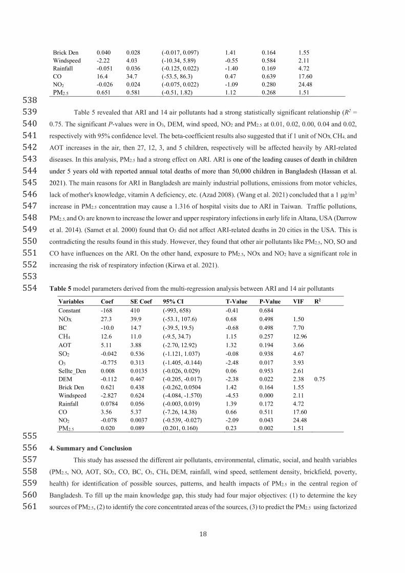
Table 5 revealed that ARI and 14 air pollutants had a strong statistically significant relationship (R2 = 539

0.75. The significant P-values were in O3, DEM, wind speed, NO2 and PM2.5 at 0.01, 0.02, 0.00, 0.04 and 0.02, 540

respectively with 95% confidence level. The beta-coefficient results also suggested that if 1 unit of NOx, CH4, and 541

AOT increases in the air, then 27, 12, 3, and 5 children, respectively will be affected heavily by ARI-related 542

diseases. In this analysis, PM2.5 had a strong effect on ARI. ARI is one of the leading causes of death in children 543

under 5 years old with reported annual total deaths of more than 50,000 children in Bangladesh (Hassan et al. 544

2021). The main reasons for ARI in Bangladesh are mainly industrial pollutions, emissions from motor vehicles, 545

lack of mother's knowledge, vitamin A deficiency, etc. (Azad 2008). (Wang et al. 2021) concluded that a 1 µg/m3 546

increase in PM2.5 concentration may cause a 1.316 of hospital visits due to ARI in Taiwan. Traffic pollutions, 547

PM2.5, and O3 are known to increase the lower and upper respiratory infections in early life in Altana, USA (Darrow 548

et al. 2014). (Samet et al. 2000) found that O3 did not affect ARI-related deaths in 20 cities in the USA. This is 549

contradicting the results found in this study. However, they found that other air pollutants like PM2.5, NO, SO and 550

CO have influences on the ARI. On the other hand, exposure to PM2.5, NOx and NO2 have a significant role in 551

increasing the risk of respiratory infection (Kirwa et al. 2021). 552

553

Table 5 model parameters derived from the multi-regression analysis between ARI and 14 air pollutants 554

Variables Coef SE Coef 95% CI T-Value P-Value VIF R2

Constant -168 410 (-993, 658) -0.41 0.684

NOx 27.3 39.9 (-53.1, 107.6) 0.68 0.498 1.50

BC -10.0 14.7 (-39.5, 19.5) -0.68 0.498 7.70

CH4 12.6 11.0 (-9.5, 34.7) 1.15 0.257 12.96

AOT 5.11 3.88 (-2.70, 12.92) 1.32 0.194 3.66

SO2 -0.042 0.536 (-1.121, 1.037) -0.08 0.938 4.67

O3 -0.775 0.313 (-1.405, -0.144) -2.48 0.017 3.93

Sellte_Den 0.008 0.0135 (-0.026, 0.029) 0.06 0.953 2.61

DEM -0.112 0.467 (-0.205, -0.017) -2.38 0.022 2.38 0.75

Brick Den 0.621 0.438 (-0.262, 0.0504 1.42 0.164 1.55

Windspeed -2.827 0.624 (-4.084, -1.570) -4.53 0.000 2.11

Rainfall 0.0784 0.056 (-0.003, 0.019) 1.39 0.172 4.72

CO 3.56 5.37 (-7.26, 14.38) 0.66 0.511 17.60

NO2 -0.078 0.0037 (-0.539, -0.027) -2.09 0.043 24.48

PM2.5 0.020 0.089 (0.201, 0.160) 0.23 0.002 1.51

555

4. Summary and Conclusion 556

This study has assessed the different air pollutants, environmental, climatic, social, and health variables 557

(PM2.5, NO, AOT, SO2, CO, BC, O3, CH4, DEM, rainfall, wind speed, settlement density, brickfield, poverty, 558

health) for identification of possible sources, patterns, and health impacts of PM2.5 in the central region of 559

Bangladesh. To fill up the main knowledge gap, this study had four major objectives: (1) to determine the key 560

sources of PM2.5, (2) to identify the core concentrated areas of the sources, (3) to predict the PM2.5 using factorized 561

19

data, and (4) to investigate the impacts of child mortality and ARI due to PM2.5 and other air pollutants. The main 562

outcomes of the study are as follows: 563

• GIS, PMF, SOM, machine learning, and multi-regression analysis derived reliable outcomes for the 564

study. 565

• PM2.5 was correlated positively with NO (0.55), BC (0.45), CH4 (0.38) and NOx (0.22), while 566

correlated negatively with rainfall (-0.10), CO (-0.33), and SO2 (-0.24). 567

• In PMF modeling, the R2 values of settlement density (1.00), SO2 (0.99), DEM (0.94), Rainfall 568

(0.77), NO (0.74) and Brickfield density (0.66) were found to be the most correlated and signified 569

variables. 570

• Factor 1 (NO, CO, Rainfall, O3, AOT, CH4, and BC) and Factors 2 (SO2, settlement density, and 571

DEM) were dominant in identifying the key sources of PM2.5, while Factor 3 was dominated by only 572

population density and brickfield. 573

• The central parts of Dhaka, the northern parts of Munshiganj, the western parts of Narshingdi and 574

Narayanganj, and the southern parts of Gazipur districts were the highly concentrated areas due to 575

diverse pollutant sources. 576

• In SOM mapping, most of the variables were concentrated in the north-eastern, central, and south-577

eastern parts of the study area, where NOx, CH4, AOT, CO, settlement density, DEM, NO, Poverty, 578

and PM2.5 have similar concentration patterns. 579

• The prediction of PM2.5 using machine learning was significant, showing reasonable R2 for random 580

forest (0.85), extreme gradient boosting (0.81) and stepwise linear (0.76). 581

• The impact of PM2.5 on child ARI was significant (p=0.002) while the R2 was 0.75. However, the 582

impacts of PM2.5 on child mortality was not significant (p=0.268) while the R2 was 0.55. However, 583

other variables like BC, CH4, settlement density, O3, DEM, wind speed, and NO2 were critical for 584

both child mortality and ARI. 585

586

In a country like Bangladesh, where air pollution and PM2.5 data are limited and sparse, the results found 587

in this study will be useful for local and regional level PM2.5 mitigation and implementation plans. The government 588

of Bangladesh, concerned ministries, UN bodies, and local and international NGOs may use these outputs for 589

reducing health impacts (particularly child mortality and ARI), and for enhancing the environmental health in the 590

study area as well as in the region. In addition to this, the overall methodology used can be replicated in similar 591

urban and semi-urban settings with additional data. Future studies should also utilize additional data and 592

parameters on ecological, seasonal air pollutants, and economic factors. 593

594

595

Supplementary Information a supplementary data sheet is attached to the main paper. 596

597

Acknowledgements The authors also deeply acknowledge to NASA and EPA for their freely available datasets. 598

599

Author contribution- Shareful: model conceptualization, methodology, data collection, analysis, writing the 600

original draft. Rahman: review and editing. Amir: methodology and editing, Saify: analysis and writing. 601

20

Funding The authors declare that no funds, grants, or other support were received during the preparation of this 602

manuscript. 603

Data availability- All data generated or analysed during the current study are presented in this article. However, 604

the raw data will be also accessible from the corresponding author. 605

Code Availability Not applicable. 606

607

Declarations 608

Conflict of interest The authors declare that they have no known competing financial interests or personal 609

relationships that could have appeared to influence the work reported in this paper. 610

Ethical Approval We certify that this manuscript is original and has not been published and will not be 611

submitted elsewhere for publication. This study follows all ethical practices during its writing. 612

Consent to Participate All authors duly participated. 613

Consent for Publication This is confirmed that the publication of this manuscript has been approved by all co-614

authors 615

616

617

618

619

Reference: 620

621

1. Adães J, Pires JCM (2019) Analysis and modelling of PM2.5 temporal and spatial behaviors in 622

European cities. Sustain 11:. https://doi.org/10.3390/su11216019 623

2. Ahmed S, Hossain I (2008) Applicability of Air pollution Modeling in a Cluster of Brickfields in 624

Bangladesh. Chem Eng Res Bull 12:28–34. https://doi.org/10.3329/cerb.v12i0.1495 625

3. Al Nayeem A, Sahadat Hossain M, Kamruzzaman Majumder A, Carter WS (2019) Spatiotemporal 626

Variation of Brick Kilns and it’s relation to Ground-level PM2.5 through MODIS Image at Dhaka 627

District, Bangladesh. Int J Environ Pollut Environ Model 2:277–284 628

4. Andersen ZJ, Bønnelykke K, Hvidberg M, et al (2012) Long-term exposure to air pollution and asthma 629

hospitalisations in older adults: A cohort study. Thorax 67:6–11. https://doi.org/10.1136/thoraxjnl-630

2011-200711 631

5. Anwar A, Ullah I, Younis M, Flahault A (2021) Impact of air pollution (PM2.5) on child mortality: 632

Evidence from sixteen asian countries. Int J Environ Res Public Health 18:. 633

https://doi.org/10.3390/ijerph18126375 634

6. Azad KMAK (2008) Risk Factors for Acute Respiratory Infections (ARI) Among Under-five Children 635

in Bangladesh. J Sci Res 1:72–81. https://doi.org/10.3329/jsr.v1i1.1055 636

7. Badyda AJ, Grellier J, Dąbrowiecki P (2017) Ambient PM2.5 exposure and mortality due to lung 637

cancer and cardiopulmonary diseases in polish cities. Adv Exp Med Biol 944:9–17. 638

https://doi.org/10.1007/5584_2016_55 639

8. BBS (2020) Upazila specific population data. In: Bangladesh Bur. Stat. http://www.bbs.gov.bd/. 640

Accessed 25 Jul 2020 641

21

9. Beelen R, Raaschou-Nielsen O, Stafoggia M, et al (2014) Effects of long-term exposure to air pollution 642

on natural-cause mortality: An analysis of 22 European cohorts within the multicentre ESCAPE 643

project. Lancet 383:785–795. https://doi.org/10.1016/S0140-6736(13)62158-3 644

10. Begum BA (2016) Dust Particle (PM10 and PM2.5) Monitoring for Air Quality Assessment in 645

Naryanganj and Munshiganj , Bangladesh. Nucl Sci Appl 25:45–47 646

11. Begum BA, Hopke PK (2018) Ambient air quality in dhaka bangladesh over two decades: Impacts of 647

policy on air quality. Aerosol Air Qual Res 18:1910–1920. https://doi.org/10.4209/aaqr.2017.11.0465 648

12. Begum BA, Hopke PK (2019) Identification of sources from chemical characterization of fine 649

particulate matter and assessment of ambient air quality in Dhaka, Bangladesh. Aerosol Air Qual Res 650

19:118–128. https://doi.org/10.4209/aaqr.2017.12.0604 651

13. Begum BA, Tazmin A, Rabbani K, et al (2009) Investigation of Sources of Particulate Matter from the 652

Tajgaon Industrial Area, Dhaka. J Bangladesh Acad Sci 33:71–85. 653

https://doi.org/10.3329/jbas.v33i1.2952 654

14. Bishop CM (2017) Sparse Additive Gaussian Process with Soft Interactions. Open J Stat 7: 655

15. Cesaroni G, Forastiere F, Stafoggia M, et al (2014) Long term exposure to ambient air pollution and 656

incidence of acute coronary events: Prospective cohort study and meta-analysis in 11 european cohorts 657

from the escape project. BMJ 348:. https://doi.org/10.1136/bmj.f7412 658

16. Chen C, Ye W, Zuo Y, et al (2019a) Graph Networks as a Universal Machine Learning Framework for 659

Molecules and Crystals. Chem Mater 31:3564–3572. https://doi.org/10.1021/acs.chemmater.9b01294 660

17. Chen G, Li S, Knibbs LD, et al (2018) A machine learning method to estimate PM2.5 concentrations 661

across China with remote sensing, meteorological and land use information. Sci Total Environ 636:52–662

60. https://doi.org/10.1016/j.scitotenv.2018.04.251 663

18. Chen XC, Ward TJ, Cao JJ, et al (2019b) Source identification of personal exposure to fine particulate 664

matter (PM2.5) among adult residents of Hong Kong. Atmos Environ 218:116999. 665

https://doi.org/10.1016/j.atmosenv.2019.116999 666

19. Cho B, Song M (2017) Distributions and Origins of PM10 in Jeollabuk-do from 2010 to 2015. J 667

Korean Soc Atmos Environ 33:251–264. https://doi.org/10.5572/kosae.2017.33.3.251 668

20. Chueinta W, Hopke PK, Paatero P (2000) Investigation of sources of atmospheric aerosol at urban and 669

suburban residential areas in Thailand by positive matrix factorization. Atmos Environ 34:3319–3329. 670

https://doi.org/10.1016/S1352-2310(99)00433-1 671

21. Dai H, Huang G, Zeng H, Yang F (2021) PM2.5 concentration prediction based on spatiotemporal 672

feature selection using XGBoost-MSCNN-GA-LSTM. Sustain 13:. 673

https://doi.org/10.3390/su132112071 674

22. Darrow LA, Klein M, Dana Flanders W, et al (2014) Air pollution and acute respiratory infections 675

among children 0-4 years of age: An 18-year time-series study. Am J Epidemiol 180:968–977. 676

https://doi.org/10.1093/aje/kwu234 677

23. Deters JK, Zalakeviciute R, Gonzalez M, Rybarczyk Y (2017) Modeling PM2.5 Urban Pollution Using 678

Machine Learning and Selected Meteorological Parameters. 2017: 679

24. DoE (2022) 700 illegal brickfields to be demolished to check air pollution. In: Bangladesh Dep. 680

Environ. https://www.thefinancialexpress.com.bd/national/700-illegal-brickfields-to-be-demolished-to-681

22

check-air-pollution-1610427426 682

25. Dominici F, Daniels M, Zeger SL, Samet JM (2002) Air pollution and mortality: Estimating regional 683

and national dose-response relationships. J Am Stat Assoc 97:100–111. 684

https://doi.org/10.1198/016214502753479266 685

26. Doreswamy, Harishkumar KS, Km Y, Gad I (2020) Forecasting Air Pollution Particulate Matter 686

(PM2.5) Using Machine Learning Regression Models. Procedia Comput Sci 171:2057–2066. 687

https://doi.org/10.1016/j.procs.2020.04.221 688

27. Dyson LL (2015) A heavy rainfall sounding climatology over Gauteng, South Africa, using self-689

organising maps. Clim Dyn 45:3051–3065. https://doi.org/10.1007/s00382-015-2523-3 690

28. Eeftens M, Tsai MY, Ampe C, et al (2012) Spatial variation of PM2.5, PM10, PM2.5 absorbance and 691

PMcoarse concentrations between and within 20 European study areas and the relationship with NO2 - 692

Results of the ESCAPE project. Atmos Environ 62:303–317. 693

https://doi.org/10.1016/j.atmosenv.2012.08.038 694

29. Egondi T, Ettarh R, Kyobutungi C, et al (2018) Exposure to outdoor particles (PM2.5) and associated 695

child morbidity and mortality in socially deprived neighborhoods of Nairobi, Kenya. Atmosphere 696

(Basel) 9:1–12. https://doi.org/10.3390/atmos9090351 697

30. Feng X, Li Q, Zhu Y, et al (2015) Artificial neural networks forecasting of PM2.5 pollution using air 698

mass trajectory based geographic model and wavelet transformation. Atmos Environ 107:118–128. 699

https://doi.org/10.1016/j.atmosenv.2015.02.030 700

31. Fotheringham AS, Charlton ME, Brunsdon C (2019) Geographically weighted regression: a natural 701

evolution of the expansion method for spatial data analysis. Trans GIS 1:. https://doi.org/DOI: 702

10.1111/tgis.12580 703

32. Gaita SM, Boman J, Gatari MJ, et al (2014) Source apportionment and seasonal variation of PM2.5 in a 704

sub-Saharan African city: Nairobi, Kenya. Atmos Chem Phys 14:9977–9991. 705

https://doi.org/10.5194/acp-14-9977-2014 706

33. Godoy ARL, Silva AEA da, Bueno MC, et al (2021) Application of machine learning algorithms to 707

PM2.5 concentration analysis in the state of São Paulo, Brazil. Brazilian J Environ Sci 56:152–165. 708

https://doi.org/10.5327/z21769478782 709

34. Han S, Sun B (2019) Impact of population density on PM2.5 concentrations: A case study in Shanghai, 710

China. Sustain 11:1–16. https://doi.org/10.3390/su11071968 711

35. Haque MI, Nahar K, Kabir MH, Salam A (2018) Particulate black carbon and gaseous emission from 712

brick kilns in Greater Dhaka region, Bangladesh. Air Qual Atmos Heal 11:925–935. 713

https://doi.org/10.1007/s11869-018-0596-y 714

36. Hasan M, Rahman S, Paul N, et al (2013) Analysis of Exhaust Emission of Vehicles in Dhaka City of 715

Bangladesh. Glob J Sci Forntier Res 13:1–6 716

37. Hasan R, Hiya HJ, Marzia S (2020) Atmospheric Content of Particulate Matter PM2.5 in Gazipur and 717

Mymensingh City Corporation Area of Bangladesh. Int J Res Environ Sci 6:. 718

https://doi.org/10.20431/2454-9444.0602003 719

38. Hassan MM, Juhász L, Southworth J (2019) Mapping time-space brickfield development dynamics in 720

Peri-Urban Area of Dhaka, Bangladesh. ISPRS Int J Geo-Information 8:. 721

23

https://doi.org/10.3390/ijgi8100447 722

39. Hassan MZ, Monjur MR, Biswas MAAJ, et al (2021) Antibiotic use for acute respiratory infections 723

among under-5 children in Bangladesh: A population-based survey. BMJ Glob Heal 6:1–13. 724

https://doi.org/10.1136/bmjgh-2020-004010 725

40. Hassan S (2022) Assessment of Health Impacts of Particulate Matter (PM2.5 ) on the Vulnerable 726

Groups in the Central part of Bangladesh. 1–24 727

41. Hoek G, Krishnan RM, Beelen R, et al (2013) Long-term air pollution exposure and cardio-respiratory 728

mortality: A review. Environ Heal A Glob Access Sci Source 12:. https://doi.org/10.1186/1476-069X-729

12-43 730

42. Hossain Bhuiyan MA, Chandra Karmaker S, Bodrud-Doza M, et al (2021) Enrichment, sources and 731

ecological risk mapping of heavy metals in agricultural soils of dhaka district employing SOM, PMF 732

and GIS methods. Chemosphere 263:128339. https://doi.org/10.1016/j.chemosphere.2020.128339 733

43. Howell CR, Su W, Nassel AF, et al (2020) Area based stratified random sampling using geospatial 734

technology in a community-based survey. BMC Public Health 20:1–9. https://doi.org/10.1186/s12889-735

020-09793-0 736

44. Hu X, Belle JH, Meng X, et al (2017) Estimating PM2.5 Concentrations in the Conterminous United 737

States Using the Random Forest Approach Department of Environmental Health , Rollins School of 738

Public Health , Emory University , Department of Biostatistics & Bioinformatics , Rollins School of. 739

Environ Sci Technol 1–29 740

45. Huang L, Zhang C, Bi J (2017) Development of land use regression models for PM2.5, SO2, NO2 and 741

O3 in Nanjing, China. Environ Res 158:542–552. https://doi.org/10.1016/j.envres.2017.07.010 742

46. IQAIR (2022) Air quality in Bangladesh. https://www.iqair.com/bangladesh 743

47. Iqbal A, Afroze S, Rahman MM (2020) Vehicular PM emissions and urban public health sustainability: 744

A probabilistic analysis for Dhaka City. Sustainability 12:1–18. https://doi.org/10.3390/SU12156284 745

48. Jiang N, Scorgie Y, Hart M, et al (2017) Visualising the relationships between synoptic circulation type 746

and air quality in Sydney, a subtropical coastal-basin environment. Int J Climatol 37:1211–1228. 747

https://doi.org/10.1002/joc.4770 748

49. Joharestani MZ, Cao C, Ni X, et al (2019) PM2.5 prediction based on random forest, XGBoost, and 749

deep learning using multisource remote sensing data. Atmosphere (Basel) 10:12–18. 750

https://doi.org/10.3390/atmos10070373 751

50. Katurji M, Noonan B, Zawar-Reza P, et al (2015) Characteristics of the springtime alpine valley 752

atmospheric boundary layer using self-organizing maps. J Appl Meteorol Climatol 54:2077–2085. 753

https://doi.org/10.1175/JAMC-D-14-0317.1 754

51. Khan MR, Huq S, Risha AN, Alam SS (2021) High-density population and displacement in 755

Bangladesh. Science (80-. ). 372:1–5 756

52. Kim S, Kim TY, Yi SM, Heo J (2018) Source apportionment of PM2.5 using positive matrix 757

factorization (PMF) at a rural site in Korea. J Environ Manage 214:325–334. 758

https://doi.org/10.1016/j.jenvman.2018.03.027 759

53. Kirwa K, Eckert CM, Vedal S, et al (2021) Ambient air pollution and risk of respiratory infection 760

among adults: Evidence from the multiethnic study of atherosclerosis (MESA). BMJ Open Respir Res 761

24

8:1–10. https://doi.org/10.1136/bmjresp-2020-000866 762

54. Kohonen T (1982) Self-Organized Formation of Topologically Correct Feature Maps. Biol Cybern 763

43:59–69 764

55. Li G, Li L, Liu D, et al (2021) Effect of PM2.5 pollution on perinatal mortality in China. Sci Rep 11:1–765

12. https://doi.org/10.1038/s41598-021-87218-7 766

56. Liang CS, Yu TY, Chang YY, et al (2013) Source apportionment of PM2.5 particle composition and 767

submicrometer size distribution during an Asian dust storm and non-dust storm in Taipei. Aerosol Air 768

Qual Res 13:545–554. https://doi.org/10.4209/aaqr.2012.06.0161 769

57. Lin GY, Chen HW, Chen BJ, Yang YC (2022) Characterization of temporal PM2.5, nitrate, and sulfate 770

using deep learning techniques. Atmos Pollut Res 13:101260. 771

https://doi.org/10.1016/j.apr.2021.101260 772

58. Lin Y, Kuwayama DP (2016) Using satellite imagery and GPS technology to create random sampling 773

frames in high risk environments. Int J Surg 32:123–128. https://doi.org/10.1016/j.ijsu.2016.06.044 774

59. Liu T, Hu B, Yang Y, et al (2020) Characteristics and source apportionment of PM2.5 on an island in 775

Southeast China: Impact of sea-salt and monsoon. Atmos Res 235:104786. 776

https://doi.org/10.1016/j.atmosres.2019.104786 777

60. Liu Y, Weisberg RH, Mooers CNK (2006) Performance evaluation of the self-organizing map for 778

feature extraction. J Geophys Res Ocean 111:1–14. https://doi.org/10.1029/2005JC003117 779

61. M.M. H, M.A. R, B. M, et al (2018) Assessment of nitrogen oxides and sulphur dioxide content in the 780

ambient air near the garments industries of Bangladesh. Environ Soc Sci 5:3–6 781

62. Ma B, Meng F, Yan G, et al (2020a) Diagnostic classification of cancers using extreme gradient 782

boosting algorithm and multi-omics data. Comput Biol Med 121:103761. 783

https://doi.org/10.1016/j.compbiomed.2020.103761 784

63. Ma J, Yu Z, Qu Y, et al (2020b) Application of the xgboost machine learning method in PM2.5 785

prediction: A case study of Shanghai. Aerosol Air Qual Res 20:128–138. 786

https://doi.org/10.4209/aaqr.2019.08.0408 787

64. Maduekwe E, de Vries WT (2019) Random spatial and systematic random sampling approach to 788

development survey data: Evidence from field application in Malawi. Sustainability 11:. 789

https://doi.org/10.3390/SU11246899 790

65. Michel TM (1997) Does Machine Learning Really Work? AI Mag 18:71–83 791

66. Miller L, Xu X (2018) Ambient PM2.5 Human Health Effects—Findings in China and Research 792

Directions. Atmosphere (Basel) 9:424. https://doi.org/10.3390/atmos9110424 793

67. Minh VTT, Tin TT, Hien TT (2021) PM2.5 Forecast System by Using Machine Learning and WRF 794

Model, A Case Study: Ho Chi Minh City, Vietnam. Aerosol Air Qual Res 21:210108. 795

https://doi.org/10.4209/aaqr.210108 796

68. Muindi K, Kimani-Murage E, Egondi T, et al (2016) Household air pollution: Sources and exposure 797

levels to fine particulate matter in Nairobi slums. Toxics 4:12–14. 798

https://doi.org/10.3390/toxics4030012 799

69. Mukta TA, Hoque MMM, Sarker ME, et al (2020) Seasonal variations of gaseous air pollutants (SO2, 800

NO2, O3, CO) and particulates (PM2.5, PM10) in Gazipur: An industrial city in Bangladesh. Adv 801

25

Environ Technol 6:195–209. https://doi.org/10.22104/AET.2021.4890.1320 802

70. Nahar N, Mahiuddin S, Hossain Z (2021) The Severity of Environmental Pollution in the Developing 803

Countries and Its Remedial Measures. Earth 2:124–139. https://doi.org/10.3390/earth2010008 804

71. Nakagawa K, Yu ZQ, Berndtsson R, Hosono T (2020) Temporal characteristics of groundwater 805

chemistry affected by the 2016 Kumamoto earthquake using self-organizing maps. J Hydrol 806

582:124519. https://doi.org/10.1016/j.jhydrol.2019.124519 807

72. Nava S, Calzolai G, Chiari M, et al (2020) Source apportionment of PM2.5 in Florence (Italy) by PMF 808

analysis of aerosol composition records. Atmosphere (Basel) 11:1–16. 809

https://doi.org/10.3390/ATMOS11050484 810

73. Naz S, Page A, Agho KE (2015) Household air pollution and under-five mortality in Bangladesh 811

(2004–2011). Int J Environ Res Public Health 12:12847–12862. 812

https://doi.org/10.3390/ijerph121012847 813

74. Ni X, Cao C, Zhou Y, et al (2018) Spatio-temporal pattern estimation of PM2.5 in Beijing-Tianjin-814

Hebei Region based on MODIS AOD and meteorological data using the back propagation neural 815

network. Atmosphere (Basel) 9:. https://doi.org/10.3390/atmos9030105 816

75. Nouri A, Ghanbarzadeh Lak M, Valizadeh M (2021) Prediction of PM2.5 Concentrations Using 817

Principal Component Analysis and Artificial Neural Network Techniques: A Case Study: Urmia, Iran. 818

Environ Eng Sci 38:89–98. https://doi.org/10.1089/ees.2020.0089 819

76. Paatero P (1997) Least square formulation of robust non-negetive factor analysis. Chemom Intell Lab 820

Syst 37:23.35 821

77. Paatero P, Tapper U (1994) Positive matrix factorization: A non-negative factor model with optimal 822

utilization of error estimates of data values. Environmetrics 5:111–126. 823

https://doi.org/10.1002/env.3170050203 824

78. Pan B (2018) Application of XGBoost algorithm in hourly PM2.5 concentration prediction. In: IOP 825

Conference Series: Earth and Environmental Science 826

79. Pavel MRS, Zaman SU, Jeba F, et al (2021) Long-Term (2003–2019) Air Quality, Climate Variables, 827

and Human Health Consequences in Dhaka, Bangladesh. Front Sustain Cities 3:. 828

https://doi.org/10.3389/frsc.2021.681759 829

80. Pearce JL, Waller LA, Chang HH, et al (2014) Using self-organizing maps to develop ambient air 830

quality classifications: a time series example. Environ Heal 13:. https://doi.org/doi:10.1186/1476-831

069X-13-56 832

81. Raaschou-Nielsen O, Andersen ZJ, Beelen R, et al (2013) Air pollution and lung cancer incidence in 17 833

European cohorts: Prospective analyses from the European Study of Cohorts for Air Pollution Effects 834

(ESCAPE). Lancet Oncol 14:813–822. https://doi.org/10.1016/S1470-2045(13)70279-1 835

82. Rahman AM (2022) CO2 Emission from Brickfields in Bangladesh: Can Ethical Responsibility by 836

Doing Reduce Level of Emission? Athens J Soc Sci 9:255–272. https://doi.org/10.30958/ajss.9-3-3 837

83. Rahman MM, Mahamud S, Thurston GD (2019) Recent spatial gradients and time trends in Dhaka, 838

Bangladesh air pollution and their human health implications. J Air Waste Manage Assoc 69:478–501. 839

https://doi.org/10.1080/10962247.2018.1548388 840

84. Rahman MM, Mazaheri M, Clifford S, Morawska L (2017) Estimate of main local sources to ambient 841

26

ultrafine particle number concentrations in an urban area. Atmos Res 194:178–189. 842

https://doi.org/10.1016/j.atmosres.2017.04.036 843

85. Saha CK, Hosain J (2016) Impact of brick kilning industry in peri-urban Bangladesh. Int J Environ 844

Stud 73:1–11. https://doi.org/10.1080/00207233.2016.1179014 845

86. Samek L, Stegowski Z, Furman L, et al (2017) Quantitative Assessment of PM2.5 Sources and Their 846

Seasonal Variation in Krakow. Water Air Soil Pollut 228:. https://doi.org/10.1007/s11270-017-3483-5 847

87. Samet JMS, Ominici FD, Urriero FCC, et al (2000) Fine particulate air pollution and mortality in 20 848

U.S. cities, 1987–1994. N Engl J Med 343: 849

88. Sharma SK, Mandal TK, Jain S, et al (2016) Source Apportionment of PM2.5 in Delhi, India Using 850

PMF Model. Bull Environ Contam Toxicol 97:286–293. https://doi.org/10.1007/s00128-016-1836-1 851

89. Srivastava D, Xu J, Vu T V., et al (2021) Insight into PM2.5sources by applying positive matrix 852

factorization (PMF) at urban and rural sites of Beijing. Atmos Chem Phys 21:14703–14724. 853

https://doi.org/10.5194/acp-21-14703-2021 854

90. Stauffer RM, Thompson AM, Young GS (2016) Tropospheric ozonesonde profiles at long-term U.S. 855

monitoring sites: 1. A climatology based on self-organizing maps. J Geophys Res Atmos 121:. 856

https://doi.org/10.1038/175238c0 857

91. Sultana M, Uddin MK (2019) Parental rejection, depression, and internet addiction among young 858

adults. Pakistan J Psychol Res 34:419–432. https://doi.org/10.33824/PJPR.2019.34.2.23 859

92. Susanna NT, Alex M, Jose J, B S (2017) Application of self organising maps (SOM) in source 860

characterization of PM10 and PM2.5 mass concentrations. In: International Conference on Recent 861

Advances in Bioresource Technology (RABT 2017) 862

93. Tallon LA, Manjourides J, Pun VC, et al (2017) Cognitive impacts of ambient air pollution in the 863

National Social Health and Aging Project (NSHAP) cohort. Environ Int 104:102–109. 864

https://doi.org/10.1016/j.envint.2017.03.019 865

94. Tan J hua, Duan J chun, Chai F he, et al (2014) Source apportionment of size segregated fine/ultrafine 866

particle by PMF in Beijing. Atmos Res 139:90–100. https://doi.org/10.1016/j.atmosres.2014.01.007 867

95. Tao S yang, Zhong B qing, Lin Y, et al (2017) Application of a self-organizing map and positive 868

matrix factorization to investigate the spatial distributions and sources of polycyclic aromatic 869

hydrocarbons in soils from Xiangfen County, northern China. Ecotoxicol Environ Saf 141:98–106. 870

https://doi.org/10.1016/j.ecoenv.2017.03.017 871

96. Thurston GD, Ito K, Lall R (2011) A source apportionment of U.S. fine particulate matter air pollution. 872

Atmos Environ 45:3924–3936. https://doi.org/10.1016/j.atmosenv.2011.04.070 873

97. Thygerson SM, Beard JD, House MJ, et al (2019) Air-quality assessment of on-site brick-kiln worker 874

housing in bhaktapur, nepal: Chemical speciation of indoor and outdoor PM2.5 pollution. Int J Environ 875

Res Public Health 16:. https://doi.org/10.3390/ijerph16214114 876

98. Tian YZ, Chen G, Wang HT, et al (2016) Source regional contributions to PM2.5 in a megacity in 877

China using an advanced source regional apportionment method. Chemosphere 147:256–263. 878

https://doi.org/10.1016/j.chemosphere.2015.12.132 879

99. Ulavi S, Shiva Nagendra SM (2019) Regression modelling for predicting visibility in a tropical urban 880

environment. WIT Trans Ecol Environ 236:149–157. https://doi.org/10.2495/AIR190151 881

27

100. UNICEF (2022) Key demographic indicators in Bangladesh. In: Unicef. 882

https://data.unicef.org/country/bgd/. Accessed 18 May 2022 883

101. USEPA (2014) EPA Positive Matrix Factorization (PMF) 5.0 Fundamentals and User Guide 884

102. Waked A, Favez O, Alleman LY, et al (2014) Source apportionment of PM10 in a north-western 885

Europe regional urban background site (Lens, France) using positive matrix factorization and including 886

primary biogenic emissions. Atmos Chem Phys 14:3325–3346. https://doi.org/10.5194/acp-14-3325-887

2014 888

103. Wang F, Chen T, Chang Q, et al (2021) Respiratory diseases are positively associated with PM2.5 889

concentrations in different areas of Taiwan. PLoS One 16:1–11. 890

https://doi.org/10.1371/journal.pone.0249694 891

104. Wu J, Xie W, Li W, Li J (2015) Effects of urban landscape pattern on PM2.5 Pollution-A Beijing Case 892

Study. PLoS One 10:1–20. https://doi.org/10.1371/journal.pone.0142449 893

105. Yazdi MD, Kuang Z, Dimakopoulou K, et al (2020) Predicting fine particulate matter (PM2.5) in the 894

greater london area: An ensemble approach using machine learning methods. Remote Sens 12:. 895

https://doi.org/10.3390/rs12060914 896

106. Yu X, Venecek M, Kumar A, et al (2019) Regional sources of airborne ultrafine particle number and 897

mass concentrations in California. Atmos Chem Phys 19:14677–14702. https://doi.org/10.5194/acp-19-898

14677-2019 899

107. Zhang L, Wang S, Wang L, et al (2015) Updated emission inventories for speciated atmospheric 900

mercury from anthropogenic sources in China. Environ Sci Technol 49:3185–3194. 901

https://doi.org/10.1021/es504840m 902

108. Zhang R, Jing J, Tao J, et al (2013) Chemical characterization and source apportionment of PM2.5 in 903

Beijing: Seasonal perspective. Atmos Chem Phys 13:7053–7074. https://doi.org/10.5194/acp-13-7053-904

2013 905

109. Zhao Z, Lao X, Gu H, et al (2021) How does air pollution affect urban settlement of the floating 906

population in China? New evidence from a push-pull migration analysis. BMC Public Health 21:1–15. 907

https://doi.org/10.1186/s12889-021-11711-x 908

909

910

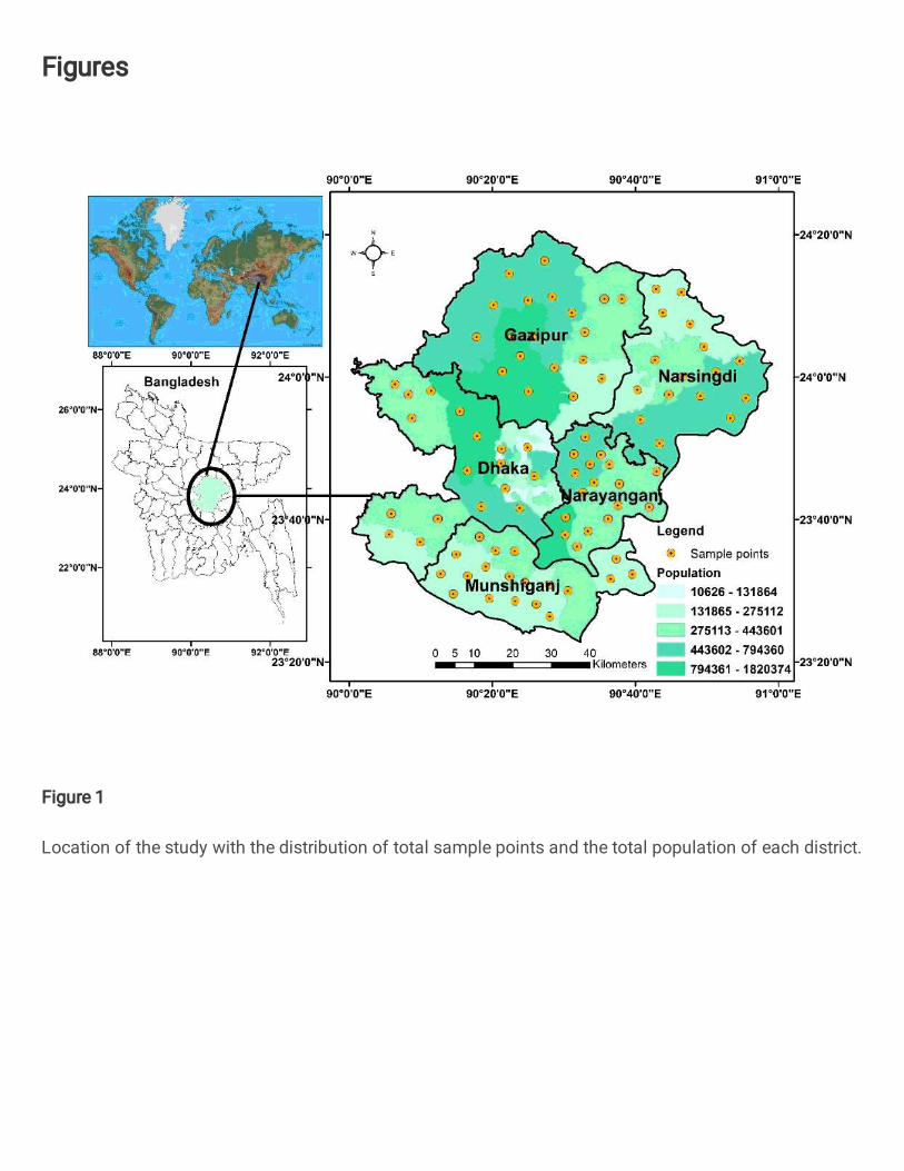
Figures

Figure 1

Location of the study with the distribution of total sample points and the total population of each district.

Figure 2

Results of Spearman’s Correlation of all variables, where *p < .05, **p < .01, ***p < .001

Figure 3

Relationship between the observed and predicted of each pollutant generated from the PMF modeling.  

Figure 4

Factor pro�le and source contribution from the PMF modeling.

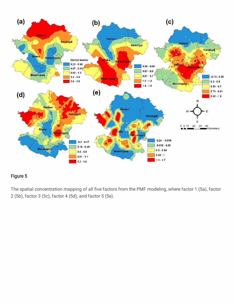
Figure 5

The spatial concentration mapping of all �ve factors from the PMF modeling, where factor 1 (5a), factor2 (5b), factor 3 (5c), factor 4 (5d), and factor 5 (5e).

Figure 6

The spatial concentration of SOM map of all variables derived from the PMF modeling, tagging NOx (a),BC (b), CH4 (c), AOT (d), CO (e), SO2 (f), O3 (g), Settlement density (h), DEM (i), NO (j), Brick�eld (k),Poverty (l), Windspeed (m), Rainfall (n) and PM2.5 (o).

Figure 7

Scatterplot of predicted and observed values of PM2.5. Figure 7a is the Random Forest, 7b is the Extremegradient boosting while 7c is the Stepwise linear.     

Supplementary Files

This is a list of supplementary �les associated with this preprint. Click to download.

Supplementarydata.docx