Electronic copy available at: http://ssrn.com/abstract=337660

MIT Sloan School of Management

Working Paper 4389-02 April 2002

SOLVING REAL-LIFE LOCOMOTIVE SCHEDULING

PROBLEMS

Ravindra K. Ahuja, Jian Liu, James B. Orlin, Dushyant Sharma, Larry A. Shughart

© 2002 by Ravindra K. Ahuja, Jian Liu, James B. Orlin, Dushyant Sharma, Larry A. Shughart. All rights reserved. Short sections of text, not to exceed two paragraphs, may be quoted without explicit permission provided that full

credit including © notice is given to the source."

This paper also can be downloaded without charge from the Social Science Research Network Electronic Paper Collection:

http://ssrn.com/abstract_id=337660

Electronic copy available at: http://ssrn.com/abstract=337660

1

Solving Real-Life Locomotive Scheduling ProblemsRavindra K. Ahuja1, Jian Liu2, James B. Orlin3, Dushyant Sharma4, and Larry Shughart5

Abstract

The locomotive scheduling problem (or the locomotive assignment problem) is to assign a consist(a set of locomotives) to each train in a pre-planned train schedule so as to provide them sufficient powerto pull them from their origins to their destinations. Locomotive scheduling problems are among the mostimportant problems in railroad scheduling. In this paper, we report the results of a study of the locomotivescheduling problem faced by CSX Transportation, a major US railroad company. We consider theplanning version of the locomotive scheduling model (LSM), where there are multiple types oflocomotives and we need to decide the set of locomotives to be assigned to each train. We present anintegrated model that determines the set of active and deadheaded locomotives for each train, lighttraveling locomotives from power sources to power sinks, and train-to-train connections (specifyingwhich inbound train and outbound trains can directly connect). An important feature of our model is thatwe explicitly consider consist-bustings and consistency. A consist is said to be busted when the set oflocomotives coming on an inbound train is broken into subsets to be reassigned to two or more outboundtrains. A solution is said to be consistent over a week with respect to a train, if the train gets the samelocomotive assignment each day it runs. We give a mixed integer programming (MIP) formulation of theproblem that contains about 197 thousand integer variables and 67 thousand constraints. An MIP of thissize cannot be solved to optimality or near-optimality in acceptable running times using commerciallyavailable software. Using problem decomposition, integer programming, and very large-scaleneighborhood search, we developed a solution technique to solve this problem within 30 minutes ofcomputation time on a Pentium III computer. When we compared our solution with the solution obtainedby the software in-house developed by CSX, we obtained a savings of over 400 locomotives, whichtranslates into savings of over one hundred million dollars annually.

1 Ravindra K. Ahuja, Industrial and Systems Engineering, University of Florida, Gainesville, FL 32611, USA.2 Jian Liu, Industrial and Systems Engineering, University of Florida, Gainesville, FL 32611, USA.3 James B. Orlin, MIT Sloan School of Management, MIT, Cambridge, MA 02139, USA.4 Dushyant Sharma, Operations Research Center, MIT, Cambridge, MA 02139, USA.5 Larry Shughart, CSX Transportation, Jacksonville, FL 32202, USA.

Electronic copy available at: http://ssrn.com/abstract=337660

2

1. INTRODUCTION

Transportation is one of the most vital services in modern society. Transportation of goods byrailroads is an integral part of the US economy. Railroads play a leading role in multi-modal andcontainer transportation. The rail transportation industry is very rich in terms of problems that can bemodeled and solved using mathematical optimization techniques. However, research in railroadscheduling has experienced a slow growth and, until recently, most contributions used simplified modelsor had small instances failing to incorporate the characteristics of real-life applications. The strongcompetition facing rail carriers (most notably from trucking companies) and the ever increasing speed ofcomputers have motivated the use of optimization models at various levels in railroad organizations. Inaddition, recently proposed models tend to exhibit an increased level of realism. As a result, there isgrowing interest for optimization techniques in railroad problems. In the last few years, a growing body ofadvances concerning several aspects of rail freight and passenger transportation has appeared in theoperations research literature (see, for example, Jovanovic and Harker [1991], Brannlund et al. [1998],Newton et al. [1998], Cordeau et al. [1998], Sherali and Suharko [1998]). This paper concerns thedevelopment of new models and algorithms for solving real-life locomotive scheduling problems faced byUS railroad companies.

The locomotive scheduling problem (or the locomotive assignment problem) is to assign a consist(a set of locomotives) to each train in a pre-planned train schedule so as to provide them sufficient powerto pull them from their origins to their destinations. Locomotive scheduling problems are among the mostimportant problems in railroad scheduling (Florian et al. [1976], Mao and Martland [1981], Smith andSheffi [1988], Chih et al. [1990], Forbes et al. [1991], Fischetti and Toth [1997], Nou et al. [1997], andZiarati et al. [1997, 1999]). Often, locomotive availability is the constraining factor in whether a traindeparts on time. With new locomotives costing in excess of $1.8 million, it is paramount to the railroadbusiness that they be managed efficiently. The variety of types of locomotives, different types of trains,and the diverse geographic networks create very difficult combinatorial optimization problems. There arenot satisfactory algorithms to solve these problems. As a result, there are inefficiencies in locomotivemanagement, and substantial savings may be achieved through the development of better models andalgorithms. CSX Transportation has over 3,000 locomotives, which translates into a capital investment ofover $5 billion, and over $1 billion in yearly maintenance and operational costs. Our study reports animprovement of 5% in average locomotive utilization for CSX, which translates into a saving of over$100 million per year.

Locomotive scheduling problems can be studied at two levels - planning level or operational level.At the planning stage of the locomotive scheduling problem, we assign locomotive types to various trains.Typically, a railroad company has different type of locomotives with different pulling and costcharacteristics. For example, we may assign two CW44AC and one CW40-8 locomotive to a train. Butthe railroad company may have several hundred locomotives of type CW44AC and CW40-8. Of these,which specific units get assigned to the train is handled by the operational locomotive schedulingproblem. The operational locomotive scheduling model also takes into account the fueling andmaintenance needs of the locomotives, which are ignored in the planning model.

Railroad companies differ on their views of the relative importance of the planning problem versusthe operational problem. One view holds that the day-to-day variability in traffic patterns, locomotiveunreliability, changing service priorities and the wide range of train schedule operations create anenvironment that is so unpredictable that it is a futile exercise to develop a static locomotive schedulingplan. This philosophy, which we refer to as the tactical planning philosophy, would attempt to take intoaccount current conditions on an on-going basis and dynamically solve the locomotive schedulingproblem. This creates an ever changing set of solutions where particular trains may run with very

3

different consists each day, and each train may source those locomotives from a variety of inbound trains,depending on that days’ situation.

These philosophy differences carry over to many aspects of the business. Ultimately, they can besummarized in two camps: those who believe it is best to operate a scheduled railroad and those whobelieve it is best to operate a “tonnage” or tactical railroad. The first camp would hold that while runninga specific schedule the same way every time may in fact result in local inefficiencies (such as trains withvery few cars or terminals that may be over staffed on some shifts), the macro level total cost of theoperation is minimized. The second camp would hold that the total cost can be reduced by tacticallyadjusting the operation to reduce the number of local inefficiencies. These strategic approaches are linkedto the view of the role of line managers as well. The operational model based railroad requires managersto be flexible and adjust their local operations to an ever changing pattern of trains, cars, locomotives andcrews. The local managers also are expected to make quick, tactical decisions to adjust the operations toreduce inefficiencies both at the local and the network level. The planning model based railroad assumesthat managers will anchor their local operation to the foundation of regular, routine, repeatable networkoperations. Over time, they will make finite adjustments to their many sub-processes that optimize theirresponsibility area. This fine tuning of the operation is not possible in a tactical operation due to the lackof stability.

These strategic approaches are linked to the view of the role of line managers as well. Theoperational model based railroad requires managers to be flexible and adjust their local operations to anever changing pattern of trains, cars, locomotives and crews. The local managers also are expected tomake quick, tactical decisions to adjust the operations to reduce inefficiencies both at the local and thenetwork level. The planning model based railroad assumes that managers will anchor their local operationto the foundation of regular, routine, repeatable network operations. Over time, they will make smalladjustments to their many sub-processes that optimize their responsibility area. This fine tuning of theoperation is not possible in a tactical operation due to the lack of stability.

The CSX managers who sponsored this research chose to emphasize the planning part of thelocomotive assignment problem for several reasons. First of all, they believe that the planning problem isof value in running the railroad. The CSX management philosophy is to operate a scheduled railroad andbelieves the inherent value of a repeatable, routine, scheduled set of decisions will ultimately not onlyminimize total locomotive costs but also total operating costs while improving the service product.Second, the planning system could be used as part of a network planning tool to evaluate which enginesto buy in the future, and to study the impact of modifying their schedule. Third, any technology developedfor the planning problem could possibly be extended to deal with tactical decisions in an operationalsetting.

In this paper, we consider the planning version of the locomotive scheduling model (LSM). Wewill now summarize the features of the LSM to give the reader a better understanding of the problem. Alarge railroad company has a train schedule which consists of several hundred trains with different weeklyfrequencies. Some trains run each day in a week, whereas others run less frequently. At CSX, there areseveral thousand train departures per week (assuming that we may count the same train running ondifferent days multiple times). Many trains have long hauls and take several days to go from their originsto their destinations. To power these trains, CSX has several thousand locomotives of different types.Some locomotives are AC powered, some DC powered; they have different manufacturers, and some aremore powerful than others. In LSM, we assign a set of locomotives to each train in the weekly trainschedule so that each train gets sufficient tractive effort (that is, gets sufficient pulling power) andsufficient horsepower (that is, gets sufficient speed), and the assignment can be repeated indefinitely weekto week. At the same time, assigning a single locomotive to a train is undesirable because if thatlocomotive breaks down, the train gets stranded on the track and blocks the movement of other trains.

4

An additional feature of the LSM is that some locomotives may be deadheaded on trains.Deadheaded locomotives do not pull the train; they are just pulled by active locomotives from one placeto another place. Deadheading plays an important role in locomotive scheduling models since it allowsextra locomotives to be moved from the places where they are in surplus to the places where are in shortsupply. Locomotives also light travel; that is, they travel on their own between different stations toreposition themselves between two successive assignments to trains. A set of locomotives in light travelforms a group, and one locomotive in the group pulls the others from an origin station to a destinationstation. Light travel is different from deadheading of locomotives since it is not limited by the trainschedule. In general, light travel is faster than deadheading. However, light travel is more costly as a crewis required to operate the pulling locomotive, and the transportation does not generate any revenue asthere are no cars attached.

Since we assign a set of locomotives (or a consist) to trains, we need to account for consist-busting.Whenever a train arrives at its destination, its consist is either assigned to an outbound train in its entirety,or its consist goes to the pool of locomotives where new consists are formed. In the former case, we saythat there is a train-to-train connection between the inbound and outbound trains and no consist-bustingtakes place. In the latter case we say that consist-busting takes place. Consist-busting leads to mixing oflocomotives from inbound trains and regrouping them to make new consists. This is undesirable fromseveral angles. First, consist-busting requires additional locomotive time and crew time to execute themoves. Second, consist-busting often results in outbound trains getting their locomotives from severalinbound trains. If any of these inbound trains is delayed, the outbound train is also delayed, whichpotentially propagates to further delays down the line. In an ideal schedule, we try to maximize the train-to-train connections of locomotives and thus minimize consist-bustings. A major contribution of thispaper is to explicitly model the economic impacts of consist-busting, and to reduce its impacts on thesystem. Moreover, a schedule that performs a lot of consist-busting may be too complex to beimplementable in practice.

Another important feature of the locomotive scheduling model is that we want a solution that isconsistent throughout the week in terms of the locomotive assignment and train-to-train connections. If atrain runs five days a week, we want it to be assigned the same consist each day it runs. If we make atrain-to-train connection between two trains and if on three days in a week both trains run, then we wantthem to have the same train-to-train connection on all three days. Consistency of the locomotiveassignment and train-to-train connections is highly desirable from an operational point of view. Anothercontribution of our paper is that we model the effects of inconsistency, and try to reduce the inconsistencyin a schedule.

This paper reports the development of a locomotive scheduling model that models the assignmentof active and deadheaded locomotives to trains, light traveling of locomotives, consistency and consist-busting decisions in an integrated model. The objective in the model is to minimize the total cost, whichis the sum of the active locomotive costs, deadheading costs, light travel costs, consist-busting costs,locomotive usage costs, and the penalty for using single locomotive consists. The solution is required toprovide sufficient power to every train in a timely fashion to meet their prescribed schedules. We firstdescribe a mixed integer programming formulation. Unfortunately, this MIP formulation is too large to besolved to optimality or near-optimality. We solve this model heuristically using a combination oftechniques taken from linear programming, integer programming, and neighborhood search algorithms.

Locomotive scheduling problems are similar to the airline scheduling problems where one assignsplanes of different types to flight legs. The planning version of the locomotive scheduling problemstudied in this paper is similar to the well known fleet assignment model (see, for example, Subramaniumet al. [1994], Hane et al. [1995]), and the operational version of the locomotive scheduling problem issimilar to the aircraft routing problem (see, for example, Barnhart et al. [1998]). However, the locomotive

5

scheduling problem considered in this paper is substantially more difficult than the fleet assignmentmodel (FAM). In the FAM, we assign a single plane to a flight leg, but in LSM we assign a set oflocomotives to a train. In FAM, there is no deadheading, no light travel, and no consist-busting. Further,the popular and well-solved FAM models assume that the flight leg schedule is the same each day of theweek; that is, they solve the daily scheduling problem and repeat it each day of the week. But in thelocomotive scheduling problem, we need to consider the weekly schedule of trains, and train schedules donot repeat on a daily basis. Hence, the LSM is combinatorially much harder to solve than the FAM.

The locomotive division at CSX Transportation has developed in-house software for the LSMwhich was developed, refined, and improved over a period of 10 years. This software has two main parts:consist-builder and locomotive scheduler. The consist-builder assigns active consists to trains; that is,which set of locomotives will actively pull the trains. This assignment is done based on train types,geography and additional business rules. The locomotive scheduler then routes locomotives in the weeklytrain network so that each train gets the desired active consist. In order to provide the desired activeconsists to trains, deadheading of the locomotives is often necessary. The locomotive scheduler considerseach locomotive type one by one and solves a minimum cost flow problem to determine locomotive flowin the network. Breaking the LSM into two distinct parts leads to inefficiencies. When consist-builderassigns active consists, it does not take into account how locomotives will flow in the network to providethose consists to trains. When locomotive flow is determined, then consists cannot be changed. Anothersource of inefficiency in their approach is that the locomotive scheduler solved the problem onelocomotive type (or, one commodity) at a time. In addition, this approach did not handle light travel oflocomotives (which was done manually) and was unable to model consist-bustings. The planning solutionprovided by their software had very high consist-bustings. As many as 85% of the trains had their consistsbusted. Our model integrates both parts of their system into a single model, treats all locomotive typessimultaneously, and models the impacts of consist-bustings, light travel, and deadheading.

Our LSM model is substantially different than locomotive scheduling models studied previously byresearchers. Single locomotive models have been studied by Forbes et al. [1991], and Fischetti and Toth[1997]. Multicommodity flow based models for planning decisions have been studied by Florian et al.[1976], Smith and Sheffi [1988], Nou et al. [1997]. Multicommodity flow based models for operationaldecisions have been developed by Chih et al. [1990], and Ziarati et al. [1997, 1999]. Our multicommodityflow based model for planning decision has more features than any of the existing planning models.

The locomotive scheduling problem is a very large-scale combinatorial optimization problem. Weformulate it as a mixed integer programming (MIP) problem, which is essentially an integermulticommodity flow problem with side constraints. The underlying flow network is the weekly space-time network where arcs denote trains, nodes denote events (that is, arrival and departure of trains), anddifferent locomotive types define different commodities. Since we assign only integer number oflocomotives to trains, we get integer multicommodity flow problems. The constraints that the locomotivesassigned to a train must provide sufficient tonnage and horsepower and that the number of locomotives ofeach type is in limited quantity gives rise to the side constraints. In addition, our formulation has fixedcharge variables which result from modeling the light travel and consist-bustings. Even when we ignorethe consistency constraints, our formulation contains about 197 thousand integer variables and 67thousand constraints, and is too large to be solved to optimality or near-optimality using existingcommercial-level MIP software.

We developed a methodology to solve the locomotive scheduling problem heuristically. By usinglinear programming, mixed integer programming, and very large-scale neighborhood search techniques,we have attempted to obtain very good solutions of the locomotive scheduling problem. We solve theLSM in two stages. In the first stage, we modify the original problem so that all trains run seven days aweek. This approximation of the original problem allows us to handle consistency constraints

6

satisfactorily. In the second stage, we modify the solution of the first stage to solve the original problemwhere trains do not run all seven days a week. The first stage problem, though substantially smaller thanthe original problem, is still too large to be solved by the existing MIP software. The source of difficultyis the fixed charge variables introduced by modeling the light travel and consist-bustings. We developedlinear programming based greedy algorithms to determine the values of these variables. Once thesevariables were determined, the resulting MIP gave very good solutions quickly, usually within 10minutes.

We developed prototype software for our algorithms and compared our software with the in-housesoftware used by CSX. On one benchmark instance, for which CSX software required 1,614 locomotivesto satisfy the train schedule, our software required only 1,210 locomotives, thereby achieving a savings ofover 400 locomotives. We obtained similar improvements on other benchmark instances. In the solutionsobtained by the CSX software, locomotives actively pull a train about 31.3% of the time, deadhead about19.6% of the time, and idle at stations about 49.1% of the time. In the solutions obtained by our software,locomotives actively pull the train about 44.4% of the time, deadhead about 8.1% of the time, light travelabout 0.8% of the time, and idle at stations about 46.7% of the time.

This paper is organized as follows. In Section 2, we describe the problem in greater detail anddefine our notation. In Section 3, we describe the space-time network which will be the basis of all of ourformulations. Section 4 describes the MIP formulation of the problem. In Section 5, we show themotivation for solving the problem in two stages, first as a daily scheduling problem followed by theweekly scheduling problem. Section 6 describes how we solve the daily scheduling problem, and Section7 the weekly scheduling problem. In Section 8, we present a summary of our algorithmic approach.Section 9 presents the computational results of our approach and compares with the approach used at theCSX Transportation. Finally, Section 10 summarizes our contributions and outlines the future researchissues.

2. PROBLEM DETAILS

In this section, we give the details and notation of the locomotive scheduling problem used forplanning at CSX.

Train Data:

Locomotives pull a set L of trains from their origins to destinations. The train schedule is assumedto repeat from week to week. Trains have different weekly frequencies; some trains run every day, whileothers run less frequently. We will consider the same train running on different days as different trains;that is, if a train runs five days a week, we will consider it as five different trains for which all data is thesame except that they will have different departure and arrival times.

We use the index l to denote a specific train. For the planning model, the train schedule isdeterministic and pre-specified. There are three classes of trains: Auto, Merchandize, and Intermodal.Each train belongs to exactly one class. The required tonnage and horsepower is specified. The tonnage ofa train represents the minimum pulling power needed to pull the train. The tonnage depends upon thenumber of cars pulled by the train, weight of the cars, and the slope or ruling grade of that train’s route.The horsepower required by the train is its tonnage multiplied by the factor that we call the horsepowerper tonnage. The greater the horsepower per tonnage, the faster the train can move. Different classes oftrains have different horsepower per tonnage. For greater model flexibility, we allow each train to have itsown horsepower per tonnage. We associate the following data with each train l.

7

dep-time(l) : The departure time for the train l. We express this time in terms of the weekly time as thenumber of minutes past Sunday midnight. For example, if the train l leaves on Monday 6 AM, thendep-time(l) = 360; and if it leaves on Tuesday 6 AM, then dep-time(l) = 1,800.

arr-time(l) : The arrival time for train l (in the same format as the dep-time(l)).

dep-station(l) : The departure station for train l.

arr-station(l) : The arrival station for train l.

lT : Tonnage requirement of train l.

lβ : Horsepower per tonnage for train l.

lH : Horsepower requirement of train l, which is defined as l l lH Tβ= .

lE : The penalty for using a single locomotive consist for train l.

Locomotive Data:

A railroad company typically has several different types of locomotives with different pulling andcost characteristics and different number of axles (often varing from 4 to 9). Locomotives with differentcharacteristics allow railroads greater flexibility in locomotive assignments, but also make the locomotivescheduling problem substantially more difficult. We denote by K the set of all locomotive types, and usethe index k to represent a particular locomotive type. We associate the following data with each train k ∈K:

kh : Horsepower provided by a locomotive of type k.

kα : Number of axles in a locomotive of type k.

kG : Weekly ownership cost for a locomotive of type k.

kB : Fleet size of locomotives of type k, that is, the number of locomotives available for assignment.

Active and Deadheaded Locomotives:

Locomotives assigned to a train either actively pull the train or deadhead. Deadheading allows extralocomotives to be moved from places where they are in surplus to the places where they are in shortsupply. For example, more tonnage leaves a coal mine than arrives at the coal mine; so more pullingpower is needed on trains departing from the mine. This creates a demand for locomotives at the mine.Similarly, more tonnage arrives at a thermal power plant than leaves it; so more pulling power is neededon trains arriving at the power plant. This creates a surplus of locomotives at the power plant. Effectivedeadheading of locomotives reduces the total number of locomotives used and improves the averagelocomotive utilization.

We need the following data for train-locomotive type combinations:

klc : The cost incurred in assigning an active locomotive of type k to train l.

8

kld : The cost incurred in assigning a deadheaded locomotive of type k to train l.

klt : The tonnage pulling capability provided by an active locomotive of type k to train l.

The active cost klc captures the economic asset cost of the locomotive for the duration of the train

and the fuel and maintenance costs. The deadhead cost kld captures the same asset cost, a reduced

maintenance cost, and zero fuel cost. Observe that the tonnage provided by a locomotive depends uponthe train. Different train routes have different ruling grades (that is, slopes) and the pulling powerprovided by a locomotive type is affected by the ruling grade.

Also specified for each train l are three disjoint sets of locomotive types: (i) MostPreferred[l], thepreferred classes of locomotives; (ii) LessPreferred[l]: the acceptable (but not preferred) classes oflocomotives; and (iii) Prohibited[l], the prohibited classes of locomotives. CSX uses business rules basedon train types and geographical considerations to determine these classes for each train. When assigninglocomotives to a train, we can only assign locomotives from the classes listed as MostPreferred[l] andLessPreferred[l] (a penalty is associated for using LessPreferred[l]).

Light Travel:

Our model allows light travel of locomotives, that is, locomotives traveling in a group on their ownbetween different stations to reposition themselves. Similar to deadheading, light travel can be aneffective way to reposition locomotives. The light travel cost has a fixed component that depends uponthe distance of travel in the light move since we need a crew, and a variable component that depends uponthe number of locomotives light traveling.

Consist-Busting:

Consist-busting is a normal phenomenon in railroads because the needs for outgoing locomotives ata station do not precisely match the incoming needs. However, consist-busting incurs a cost in complexityof managing the system, and in delays in repositioning locomotives. Consist-busting can be reduced by abetter scheduling of locomotives. We model the cost of consist-busting with a fixed component, B, perconsist-busting and a variable component that depends upon the number of locomotives involved in theconsist-busting.

We will now describe the constraints in the LSM. The constraints can be classified into two parts:hard constraints (which each locomotive assignment must satisfy) and soft constraints (which aredesirable but not always required to be satisfied). We incorporate soft constraints by attaching a penaltyfor each violation of these constraints.

Hard Constraints:

Power requirement of trains: Each train must be assigned locomotives with at least the required tonnageand horsepower.

Locomotive type constraints: Each train l is assigned locomotive types belonging to the setMostPreferred[l] and LessPreferred[l] only.

Locomotive balance constraints: The number of incoming locomotives of each type into a station at agiven time must equal the number of outgoing locomotives of that type at that station at that time.

9

Active axles constraints: Each train must be assigned locomotives with at most 24 active axles. Thisbusiness rule is designed to protect the standard couplers used in North America. Exceeding 24 poweredaxles may result in overstressing the couplers and causing a train separation.

Consist size constraints: Each train can be assigned at most 12 locomotives including both the activeand deadheaded locomotives. This rule is a business policy of CSX that reduces its risk exposure if thetrain were to suffer a catastrophic derailment.

Fleet size constraints: The number of assigned locomotives of each type is at most the number ofavailable locomotives of that type.

Repeatability of the schedule: The number and type of locomotives positioned at each station at thebeginning of the week must equal the number and type of locomotives positioned at that station at the endof the week. This ensures that the assignment of locomotives can be repeated from week to week.

Soft Constraints:

Consistency in locomotive assignment: If a train runs five days a week, then it should be assigned thesame consist each day it runs. CSX believes that crews will perform more efficiently and more safely ifthey operate the same equipment on a particular route and train. As the crews learn the operating nuancesassociated with each combination, they will adjust their throttle and braking control accordingly.

Consistency in train-to-train connections: If locomotives carrying a train to its destination stationconnect to another train originating at that station, then it should preferably make the same connection oneach day both the trains run. This is useful to help terminal managers optimize their sub-processesassociated with arriving and departing trains.

Same class connections: Trains should connect to other trains in the same class, e.g., auto trains shouldconnect to auto trains; merchandise trains should connect to merchandise trains, etc. This is useful in thatdifferent trains have different preferred types of locomotives and may originate and terminate at differentlocations within a larger terminal area (an unloading ramp, for example).

Avoid consist-busting: Consist-busting should be avoided as much as possible.

OBJECTIVE FUNCTION:

The objective function for the locomotive scheduling model contains the following terms:

• Cost of ownership, maintenance, and fueling of locomotives• Cost of active and deadheaded locomotives • Cost of light traveling locomotives• Penalty for consist-busting• Penalty for inconsistency in locomotive assignment and train-to-train connections• Penalty for using single locomotive consists

3. SPACE-TIME NETWORK

We will formulate the locomotive scheduling problem as a multicommodity flow problem with sideconstraints on a network, which we call the weekly space-time network. Each locomotive type defines acommodity in the network. We denote the space-time network as G7 = (N7, A7), where N7 denotes thenode set and A7 denotes the arc set. We construct the weekly space-time network as follows. We create a

10

train arc (l', l") for each train l; the tail node l' of the arc denotes the event for the departure of train l atdep-station(l) and is called a departure node. The head node l" denotes the arrival event of train l at arr-station(l) and is called an arrival node. Each arrival or departure node has two attributes: place and time.For example, place(l') = dep-station(l) and time(l') = dep-time(l). Similarly, place(l") = arr-station(l) andtime(l") = arr-time(l). Some trains are called forward trains and some trains are called backward trains.Forward trains are those trains for which dep-time(l) > arr-time(l) and backward trains are those trainsfor which dep-time(l) < arr-time(l). For example, a train that leaves on Monday and arrives at itsdestination on Tuesday is a forward train; whereas a train that leaves on Saturday and arrives on Mondayis a backward train. (Recall that our timeline begins on Sunday at midnight.)

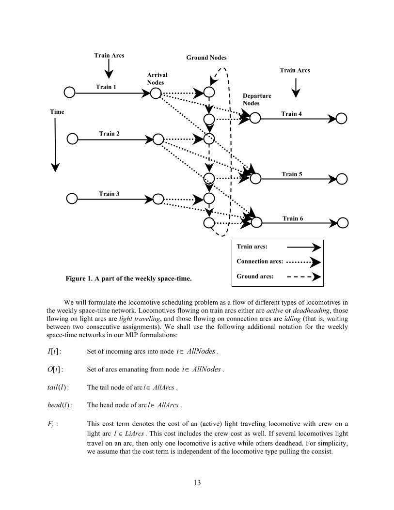
To allow the flow of locomotives from an inbound train to an outbound train, we introduce groundnodes and connection arcs. For each arrival node, we create a corresponding arrival-ground node withthe same place and time attribute as that of the arrival event. Similarly, for each departure event, wecreate a departure-ground node with the same place and time attribute as that of the departure node. Weconnect each arrival node to the associated arrival-ground node by a directed arc called the arrival-ground connection arc. We connect each departure-ground node to the associated departure node througha directed arc called the ground-departure connection arc. We next sort all the ground nodes at eachstation in the chronological order of their time attributes, and connect each ground node to the nextground node in this order through directed arcs called ground arcs. (We assume without any loss ofgenerality that ground nodes at each station have distinct time attributes.) The ground nodes at a stationrepresent the pool (or storage) of locomotives at the station at different instants of times, when events takeplace. As trains arrive, they bring in locomotives to the pool through arrival-ground connection arcs. Astrain departs, they take out locomotives from the pool through ground-departure connection arcs. Theground arcs allow inbound locomotives to stay in the pool as they wait to be connected to the outboundtrains. We also connect the last ground node in the week at a station to the first ground node of the weekat that station through the ground arc; this ground arc models the ending inventory of locomotives for aweek becoming the starting inventory for the following week.

We also model the possibility of an inbound train sending its entire consist to an outbound train.We capture this possibility by creating train-train connection arcs from an arrival node to those departurenodes whenever such a connection can be feasibly made. Railroads have some business rules about whichtrain-train connections can be feasibly made. The arrival nodes i″ for a train i can be connected to adeparture node j′ for train j provided min-connection-time ≤ dep-time(j) – arr-time(i) ≤ max-connection-time, where min-connection-time and max-connection-time are two specified parameters. For example,min-connection-time = 120 (in minutes) and max-connection-time = 480.

We also allow the possibility of light travel, that is, several locomotives forming a group andtraveling on their own as a group from one station to another station. Using a method described later inSection 6.4, we create possibilities for light travel among different stations. We create a light arc in theweekly space-time network corresponding to each light travel possibility. Each light arc originates at aground node (with a specific time and at a specific station) and also terminates at a ground node. Eachlight arc has a fixed charge which denotes the fixed cost of sending a single locomotive with crew fromthe origin of the light arc to its destination. We denote this fixed charge for a light travel arc l by Fl. Thelight arc also has a variable cost which depends upon the number of locomotives light traveling as agroup.

To summarize, the weekly space-time network G = (N, A) has three types of nodes - arrival nodes(ArrNodes), departure nodes (DepNodes), and ground nodes (GrNodes); and four kinds of arcs - train arcs(TrArcs), connection arcs (CoArcs), ground arcs (GrArcs) and light travel arcs (LiArcs). Let AllNodes =ArrNodes ∪ DepNodes ∪ GrNodes, and AllArcs = TrArcs ∪ CoArcs ∪ GrArcs ∪ LiArcs. We show in

11

Figure 1, a part of the weekly space-time network at a particular station, which illustrates various kinds ofarcs.

12

13

We will formulate the locomotive scheduling problem as a flow of different types of locomotives inthe weekly space-time network. Locomotives flowing on train arcs either are active or deadheading, thoseflowing on light arcs are light traveling, and those flowing on connection arcs are idling (that is, waitingbetween two consecutive assignments). We shall use the following additional notation for the weeklyspace-time networks in our MIP formulations:

[ ]I i : Set of incoming arcs into node i AllNodes∈ .

[ ]O i : Set of arcs emanating from node i AllNodes∈ .

( )tail l : The tail node of arc l AllArcs∈ .

( )head l : The head node of arc l AllArcs∈ .

lF : This cost term denotes the cost of an (active) light traveling locomotive with crew on alight arc l LiArcs∈ . This cost includes the crew cost as well. If several locomotives lighttravel on an arc, then only one locomotive is active while others deadhead. For simplicity,we assume that the cost term is independent of the locomotive type pulling the consist.

Train arcs:

Connection arcs:

Ground arcs:

Train Arcs

Train 1

Train 4

Train 5

ArrivalNodes

Train 2

Train 3

Train 6

DepartureNodes

Train Arcs

Ground Nodes

Time

Figure 1. A part of the weekly space-time.

14

kld : Recall that in Section 2, we defined k

ld as the cost of deadheading of locomotive type k ontrain arc l. We now define it for every arc .l AllArcs∈ For a light arc ,l LiArcs∈

kld captures the cost of traveling for a non-active locomotive of locomotive type k on arc l.

For a connection arc l CoArcs GrArcs∈ ∪ , kld captures the cost of idling for locomotive

type k on arc l.

CB: The set of all connection arcs from arrival nodes to ground nodes. These are the arcs onwhich positive flow represents consist-busting. Alternatively, CB = {(i, j) ∈ AllArcs: i ∈ArrNodes and j ∈ GrNodes}.

CheckTime : It is a time instant of the week when no event takes place; that is, no train arrives or departsat any station. We will henceforth assume that CheckTime is Sunday midnight.

S: The set of arcs that cross the CheckTime; that is, S = {(i, j) ∈ AllArcs: time(i) < CheckTime< time(j)}.

4. THE MIXED INTEGER PROGRAMMING FORMULATION

In this section, we present the mixed integer programming (MIP) formulation of the locomotivescheduling model.

Decision Variables:

klx : Integer variable representing the number of active locomotives of type k K∈ on the arc

l TrArcs∈ ;

kly : Integer variable indicating the number of non-active locomotives (deadheading, light-traveling

or idling) of type k K∈ on the arc l AllArcs∈ ;

lz : Binary variable which takes value 1 if at least one locomotive flows on the arcl LiArcs CoArcs∈ ∪ , and 0 otherwise;

lw : Binary variable which takes value 1 if there is a flow of a single locomotive on arc ,l TrArcs∈and 0 otherwise;

ks : Integer variable indicating the number of unused locomotives of type k K∈ .

Objective Function:

min k k k k k kl l l l l l l l l

l TrArcs k K l AllArcs k K l LiArcs l CB l TrArcs k Kz c x d y F z Bz E w G s

∈ ∈ ∈ ∈ ∈ ∈ ∈ ∈

= + + + + −∑ ∑ ∑ ∑ ∑ ∑ ∑ ∑ (1a)

Constraints:, for all ,k k

l l lk K

t x T l TrArcs∈

≥ ∈∑ (1b)

, for all ,k kl l l

k Kh x T l TrArcsβ

∈

≥ ∈∑ (1c)

15

24, for all ,k kl

k Ka x l TrArcs

∈

≤ ∈∑ (1d)

( ) 12, for all ,k kl l

k Kx y l TrArcs

∈

+ ≤ ∈∑ (1e)

[ ] [ ]( ) ( ), for all , for all ,k k k k

l l l ll I i l O i

x y x y i AllNodes k K∈ ∈

+ = + ∈ ∈∑ ∑ (1f)

12 , for all ,kl l

k Ky z l CoArcs LiArcs

∈

≤ ∈ ∪∑ (1g)

[ ]1, for all ,l

l O iz i ArrNodes

∈

= ∈∑ (1h)

[ ]1, for all ,l

l I iz i DepNodes

∈

= ∈∑ (1i)

( ) 2, for all ,k kl l l

k Kx y w l TrArcs

∈

+ + ≥ ∈∑ (1j)

( ) , for all ,k k k kl l

l Sx y s B k K

∈

+ + = ∈∑ (1k)

, 0 and integer, for all , for all ,k kl lx y l TrArcs k K≥ ∈ ∈ (1l)

{ }0, 1 , for all ,lz l CoArcs LiArcs∈ ∈ ∪ (1m) { }0, 1 , for all .lw l TrArcs∈ ∈ (1n)

We now give some explanation for the above formulation to show that it correctly represents theLSM. We first discuss the constraints. The constraint (1b) ensures that the locomotives assigned to a trainprovide the required tonnage, and the constraint (1c) ensures that the locomotives assigned provide therequired horsepower. The constraint (1d) models the constraint that the number of active axles assigned toa train does not exceed 24. The constraint (1e) models the constraint that every train is assigned at most12 locomotives. The flow balance constraints (1f) ensures that the number of incoming locomotives equalthe number of outgoing locomotives at every node of the weekly space-time network. The constraint (1g)makes the fixed charge variable lz equal to 1 whenever a positive flow takes place on a connection arc ora light arc; this constraint also ensures that no more than 12 locomotives flow on any light arc. Theconstraint (1h) states that, for each inbound train, all the inbound locomotives use only one connectionarc; either all the locomotives go to the associated ground node (in which case consist-busting takesplace) or all the locomotives go to another outbound train (in which case consist-busting does not takeplace and there is a train-to-train connection). The constraint (1i) states that for each outbound train all theoutbound locomotives either come from a ground node or all the locomotives come from an incomingtrain. The constraint (1j) makes the variable lw equal to 1 whenever a single locomotive consist isassigned to train l. Finally, the constraint (1k) counts the total number of locomotives used in the week;which is the sum of the flow of locomotives on all the arcs crossing the CheckTime. The differencebetween the number of locomotives available minus the number of locomotives used gives the number oflocomotives saved ( ks ).

We now discuss the objective function (1a) which contains six terms. The first term denotes thecost of actively pulling locomotives on train arcs. The second term captures the cost of deadheadinglocomotives on train and light travel arcs, and the cost of idling locomotives. We also include the variablecost of consist-busting in the definition of the term k

ld for each arc .l CB∈ The third term,

l ll LiArcsF z

∈∑ denotes the fixed cost of light traveling locomotives. The fourth term, ll CBBz

∈∑ , denotesthe fixed cost of consist-busting. The fifth term, Σl∈TrArcsElwl, denotes the penalty associated with thesingle locomotive consists; and the sixth term, Σk∈KGksk, represents the savings accrued from not using allthe locomotives.

16

Observe that the formulation (1) assumes that any locomotive type can flow on any train arc. Butrecall from our discussion in Section 2 that each train arc l has MostPreferred[l], LessPreferred[l], andProhibited[l] sets of locomotives. We handle these constraints in the following manner. To theformulation (1) we add the constraints k

lx = 0 for each k ∈ Prohibited[l] and each l ∈ TrArcs. Thisconstraint ensures that prohibited locomotives are never used on train arcs. To discourage the flow oflocomotive types belonging to the LessPreferred sets, we multiply k

lc by a suitable parameter larger than(for example, 1.2) for each k ∈ LessPreferred[l] and each l ∈ TrArcs.

Our formulation (1) incorporates all the hard constraints described in Section 2, but not all the softconstraints. The formulation does not incorporate the consistency constraints. Including those constraintswould make the formulation unmanageably large. We, however, do handle the same class constraintsimplicitly in the definition of the term k

ld . If a train-train connection arc l is not the same class connectionarc, we multiply its k

ld value by a constant parameter greater than 1, which penalizes the use of thesearcs. By suitably selecting the value of this parameter, we can satisfy the same class constraints to varyingdegrees. We can also obtain different levels of consist-busting by selecting different values of the consist-busting cost B. The greater the value of B we choose, the less will be the amount of consist-busting in anoptimal solution.

In the data provided to us by CSX, there were 538 trains, each of which operate several days in aweek, and 5 locomotive types. The weekly space-time network consisted of 8,798 nodes and 30,134 arcs.The MIP formulation (1) consisted of 197,424 variables and 67,414 constraints. This formulation couldnot be solved to optimality or near-optimality using the state of the art commercial software. As a matterof fact, we were unable to solve even the linear programming (LP) relaxation of the problem. When wesolved the LP relaxation of a much smaller problem, we found that the LP solution was highly fractional.Most of the variables were non-integer and the integer programming algorithm did not find a good integersolution in several hours. In addition, our MIP formulation (1) omits the consistency constraints that thesame train running on different days should have the same locomotive assignment. In our formulation, atrain running on different days is treated as separate trains and their locomotive assignments can be quitedifferent. In principle, we can add new constraints to enforce the consistency constraints, but that wouldbe impractical as it would increase the size of the MIP substantially. Hence, satisfying the consistencyconstraints by introducing new constraints did not seem to be a feasible option. Rather we developed analternative approach that simultaneously helped enforce consistency while dramatically reducing theproblem size. We describe our approach in the next section.

5. SIMPLIFYING THE MODEL

We next analyzed the number of trains running with different frequencies in a week for CSX. Thetable shown in Figure 2 gives these numbers. The first column in the table gives the train frequency in aweek; that is, how often the trains run in a week. The second column in the table gives the number oftrains in the train schedule with the frequency given in the first column. For example, in the trainschedule, there are 372 trains that run all seven days a week, there are 62 trains that run six days a week,and so on. The third column is a product of the first and second columns, the fourth column gives acumulative sum of the third column, and the fifth column expresses the values in the fourth column in thepercentage notation. Observe that the third column gives the number of train arcs in the weekly space-time network for trains with different frequencies. The table shows that 94% of the train arcs in the space-time network correspond to the trains that run 5, 6, or 7 days.

17

TrainFrequency

(A)Number of Trains (B) A*B

Cum.Sum of

A*BCumulative

Percentage A*B7 372 2,604 2,604 78%6 62 372 2,976 90%5 29 145 3,121 94%4 24 96 3,217 97%3 20 60 3,277 99%2 16 32 3,309 100%1 15 15 3,324 100%

Figure 2. Analysis of trains and their frequencies.

We now state an approximation that reduces the size of the MIP substantially and also helps ussatisfy the consistency constraints. We create a daily locomotive scheduling model that is a simplificationof the weekly locomotive scheduling model in the following manner. Each train with a frequency of pdays per week or larger is a train in the daily model. Each train with frequency strictly less than p days isnot included in the daily model. After some analysis and testing, we chose p = 5. So, if a train has afrequency of 4 or less in the weekly model, we eliminate it from our daily model. Our daily model isroughly seven times smaller than the weekly model, and accordingly much easier to solve. In addition,since we repeat the train’s daily schedule for each day of the week, the solution automatically satisfies theconsistency constraints. Hence this simplification achieves both of our goals, which is to reduce theproblem size and achieve consistency of the solution.

The solution to the daily model is not feasible for the weekly model. It assigns locomotives tosome train arcs that do not exist (those trains that run 5 or 6 days per week) and does not assignlocomotives to train arcs that exist (those trains that run 4 days per week or fewer). But for the CSX data,the approximation we make is relatively small compared to the size of the problem. With our choice of p= 5, we assign locomotives to 120 train arcs that do not exist in the weekly model and do not assignlocomotives to 203 train arcs that do exist in the weekly model. These numbers are small compared to thetotal number of train arcs, which is 3,324.

We take the solution for the daily model and transform it to a feasible solution to the weekly modelin a separate algorithm. We thus solve the locomotive scheduling problem in two stages. The first stagesolves the daily locomotive scheduling problem, and the second stage takes in the daily locomotiveschedule and modifies it to obtain the weekly locomotive schedule. We will in the next few sections focuson the daily locomotive scheduling problem, and return to the weekly locomotive scheduling problem inSection 7. In our investigations, we chose p = 5 primarily because the solution of the model with p = 5was more easily converted to a solution of the weekly locomotive scheduling problem than other valuesof p.

6. SOLVING THE DAILY LOCOMOTIVE SCHEDULING PROBLEM

In this section, we describe how to solve the daily scheduling problem. We describe (i) how toconstruct the daily space-time network and formulate the MIP for the daily scheduling problem; and (ii)how to solve the daily locomotive scheduling problem using a decomposition-based approach.

6.1 Constructing the Daily Space-Time Network and Formulating the MIP

The daily space-time network is constructed for the daily locomotive scheduling problem whereeach train is assumed to run each day of the week. It is constructed in a similar manner to the way in

18

which we construct the weekly space-time network. We represent the daily space-time network as G1 =(N1, A1). The daily space-time network is about seven times smaller than the weekly space-time network.

In the daily model, the departure time is the number of minutes past midnight that the train departs,and the arrival time is the number of minutes past midnight that the train arrives. The day of the weekdoes not play a role in this daily model. For a train l, let day(l) denote the number of times the train willcross the midnight time line as it goes from its origin to its destination. For example, consider a train thatleaves station A on 7 AM on one day and arrives at 4 PM two days later at Station B. For example, thetrain starts on Monday at 7 AM and arrives at 4 PM on Wednesday. In this case, day(l) = 2. If this trainwere to repeat each day in our weekly model, then two copies of the train would cross the time line atmidnight on Sunday - the train that starts at 7 AM on Saturday and ends at 4PM on Monday, and the onethat starts at 7 AM on Sunday and ends at 4 PM on Tuesday. In general, if day(l) = k in our daily model,then there are k copies of the train l that cross the midnight at Sunday time line in our weekly model.Therefore, assigning a locomotive in our daily model to a train l with day(l) = k corresponds to assigningk locomotives of the same type in the weekly model.

To account for the impact of day(l), we modify the fleet size constraint of the locomotivescheduling problem as follows:

( ) ( ) , for all .k k k kl l

l Sx y day l s B k K

∈

+ + = ∈∑

The rest of the formulation of the locomotive scheduling problem (1) on the daily space-timenetwork is identical to the one given earlier.

6.2 Solving the MIP for the Daily Scheduling Problem

Though the space-time network for the daily scheduling problem was substantially smaller than thespace-time network for the weekly scheduling problem, we found it to be too large to be solved tooptimality or near-optimality. The daily locomotive scheduling problem consisted of 463 train arcs, andthe daily space-time network contained 1,323 nodes and 30,034 arcs. The MIP formulation consisted of22,314 variables and 9,974 constraints. The LP relaxation took a few seconds to solve but the MIP did notgive any integer feasible solution in 72 hours of running time. We conjecture that the biggest source ofdifficulty was the presence of fixed charge variables zl (for connection and light arcs) which take value 1whenever there is a positive flow on arc l. It is well known that MIPs with many fixed charge variablesoften produce weak lower bounds.

In order to obtain high quality feasible solutions and to keep the total running time of the algorithmsmall, we decided to eliminate the fixed charge variables from the MIP formulation using heuristics. Theheuristics also allowed us greater flexibility in determining what kind of solution we want. In ourformulation, we have two kind of fixed charge variables – one corresponding to connection arcs, and theother corresponding to light arcs. We will first consider the fixed charge variables corresponding to theconnections arcs, followed by the fixed charge variables corresponding to light arcs. We also considersome cases in which fixed charge variables can be eliminated without any loss of generality.

6.3 Determining Train-Train Connections

Train companies often specify some “hardwired” train-train connections, that is, they specifysome inbound trains whose consist must go to the specified outbound trains. These hard-wired train-trainconnections are easy to enforce. If the inbound train i at a station is hardwired to the outbound train j atthat station, then in the space-time network we create the train-train connection arc (i″, j′) and do not

19

allow any other connection arc to emanate node i″ or enter node j′. This arc is the only connection arcleaving node i″ and the only connection arc entering node j′. This will ensure that all locomotives broughtin by the inbound train i directly go to the outbound train j without consist-busting. In this case, there willbe no fixed charge variables corresponding to the trains i and j.

Sometimes, a station has a unique inbound train and a unique outbound train. If this station has nolight traveling locomotives coming into it, then all the locomotives brought in by the inbound train will beautomatically assigned to the outbound train. Hence, there will be no consist-busting and there will be noneed for fixed charge variables. Sometimes, a station has one inbound train and two outbound trains, or ithas two inbound trains and one outbound trains. In these cases too, consist-busting cannot be avoided andthere is no need to introduce any train-train connection arcs. Again, there will not be any fixed chargevariables; all inbound train(s) send their locomotives to the ground node, and all outbound train(s) will gettheir locomotives from the ground node.

Train companies also have rules about which train-train connections are permissible or desirable.The difference between the arrival time of the inbound train and the departure time of the outbound trainmust be between some specified lower and upper bounds in order for a valid train-train connection to bemade. They also prefer connections between trains of the same class; that is, auto trains sendinglocomotives to auto trains and merchandize trains to the merchandize trains, etc. They also want that thetonnage and HP requirements of the two trains be similar in order for it to be a desirable train-trainconnection. Using these business rules, we determine the set of all “candidate” train-train connections. Inthe next step, we will “fix” some of these candidate train-train connections into hardwired train-trainconnections and all “unfixed” trains will send (or receive) locomotives to (from) ground nodes. Usingthese heuristics we eliminate fixed charge variables corresponding to consist-busting in our model.

We fix some candidate train-train connections by solving an iterative procedure that solves asequence of linear programming relaxations of the daily locomotive scheduling problem given in Section6.1 with some changes. We start with a daily space-time network containing all the candidate train-trainconnection arcs and candidate light arcs. We next solve the linear programming relaxation of thelocomotive scheduling model where there are no fixed charge variables and constraints (that is,constraints (1g) through (1i)) and all the train-to-ground and ground-to-train connections have a largecost, to discourage the flow on such arcs. This is an alternative way of discouraging consist-busting. Letα(l) denote the total flow of locomotives (of all types) on any arc l in the daily space-time network. Wenext select a candidate train-train connection arc h with the largest value of α(h). This arc indicates agood potential train-train connection. We make this connection arc the unique connection arc for the twocorresponding trains, that is, we make it mandatory for the inbound train to send its locomotive to thecorresponding outbound train, and resolve the linear programming relaxation. If this linear programmingrelaxation is infeasible or increases the cost of the new solution by an amount greater than β, we do notmake this train-train connection; otherwise we keep this connection. In any case, we remove arc h fromthe list of candidate train-train connections. This completes one iteration of our procedure to fix train-trainconnections. We select another candidate train-train connection arc h with the largest value of α(h) in thecurrent flow solution, and repeat this process until either we have reached the desired number of train-train connections (as specified by some parameter γ), or the set of candidate train-train connectionsbecomes empty.

Our method of identifying the train-train connections is a greedy method. It identifies a promisingchoice, makes it, and resolves the LP problem to assess the impact of this choice. If it turns out to be abad choice, it is ignored; otherwise, it is made. By suitably identifying the values of the two parameters βand γ, we can govern the behavior of the algorithm. By choosing the higher value of β, we can increasethe number of train-train connections. We can also increase the number of train-train connections by

20

increasing the value of the parameter γ. We show in Section 9 that using this heuristic technique we wereable to increase the number of train-train connections to 72%, which was substantially higher than thegoals originally set by our industry sponsor. In fact, 72% was originally not considered an achievablegoal. The parameters β and γ need to be assigned right values so that we get the desired consist-busting.We used β = $1,000, and varied γ to get different levels of consist-bustings.

6.4 Determining Light Travel Arcs

Light travel of locomotives plays an important role in locomotive scheduling and can substantiallyimpact the quality of the solution. Incorporating light travel in the locomotive scheduling model requirestwo decisions: (i) candidate light arcs: what should be the light travel arcs in the space-time network; and(ii) flow on light travel arcs: which locomotives will flow on the candidate light arcs. In principle, wecould allow light travel of locomotives from any station to any station at any time of the day. To captureall these possibilities of light travel in our network, we would need to add a large number of arcs in thedaily space-time network. This would increase the size of the network substantially and also the numberof flow variables. In addition, since we associate a fixed charge variable with each candidate light arc, thenumber of fixed charge variables would be very high. Rather than introducing a large number of lighttravel arcs, we developed a heuristic procedure to create a small but potentially useful collection of lighttravel arcs, and another heuristic procedure for selecting a subset of these arcs for light travel. We nowdescribe these procedures in greater detail.

Our first procedure determines the candidate light travel possibilities. For each such arc, we need todecide its origin station, its start time, its destination station, and its end time. The end time can becomputed from the origin station, its start time, and its destination station if we know the average speed ofthe light traveling locomotives. In the railroad network, light traveling locomotives typically travel from"power sources" (stations where inbound trains require substantially more tonnage/horsepower than theoutbound trains) to "power sinks" (stations where outbound trains require substantially moretonnage/horsepower than the inbound trains). We first construct the space network, which is the same asthe daily space-time network described in Section 6.1 except that we ignore the time element.Equivalently, we shrink all the station nodes with different times into a single station node. We nextdetermine the additional availability of pulling power at the power sources and the additional demand forpulling power at the power sinks in the space network of our weekly model. To incorporate bothhorsepower and tonnage constraints simultaneously, we translate this information into the number oflocomotives of some standard type, such as, SD40. This gives us node imbalances of locomotives in thespace network. We then solve a minimum cost flow problem (see, for example, Ahuja, Magnanti andOrlin [1993]) in the space network to determine the optimal locomotive flow in the network. If there is apositive flow of locomotives on arc (i, j) in the space network greater than some threshold value (say, twolocomotives), then we create candidate light travel arcs from city i to city j in the space-time networkdeparting from city i every 8 hours. For the data provided to us by CSX, we found 58 arcs in the spacenetwork with flow greater than 2 locomotives and we created 174 candidate light arcs in the space-timenetwork.

In our formulation described before, we need to create a fixed charge variable for each candidatelight arc and we cannot solve the formulation for these many fixed charge variables in the required time.Our second procedure eliminates the fixed charge variables. From the list generated by the previousheuristic, it selects a small subset of light arcs and assumes that there will be light travel on these arcs.The procedure works as follows. It first solves a linear programming formulation of the locomotivescheduling problem where all the candidate light arcs are added. It then removes all those light arcs whichhave zero flow. Let α(l) denote the total number of locomotives flowing on an arc l. We then perform thefollowing iterative step. We select the light arc l with the smallest value of flow α(l). Suppose this is arcq. We delete arc q from the network and solve the LP relaxation of the locomotive scheduling problem. If

21

the deletion of this light arc causes the total cost of flow (of the LP relaxation) to go up by at least η units,we do not delete this arc; otherwise we delete this arc and replace α by the new flow. We repeat thisprocess until there are no unexamined light arcs. The number of light arcs generated by this modulecrucially depends upon the value of the parameter η. If we increase the value of η, then we will increasethe number of arcs deleted from the network which will result in lesser number of light arcs beinggenerated. Hence, by assigning suitable values to this parameter, one can generate appropriate number oflight arcs. We used η = $1,000 in our implementation.

6.5 Determining Active and Deadheaded Locomotive Flow Variables

As described before, the use of heuristics to determine train-train connections and light travel arcseliminates the fixed charge variables. We next determine the remaining variables that are the active anddeadheaded locomotives on arcs in the network. To determine these variables, we solve the followinginteger programming problem:

min k k k k k kl l l l l l

l TrArcs k K l AllArcs k K l TrArcs k Kz c x d y E w G s

∈ ∈ ∈ ∈ ∈ ∈

= + + −∑ ∑ ∑ ∑ ∑ ∑ (2a)

subject to:

, for all ,k kl l l

k Kt x T l TrArcs

∈

≥ ∈∑ (2b)

, for all ,k kl l l

k Kh x T l TrArcsβ

∈

≥ ∈∑ (2c)

24, for all ,k kl

k Ka x l TrArcs

∈

≤ ∈∑ (2d)

( ) 12, for all ,k kl l

k Kx y l TrArcs LiArcs

∈

+ ≤ ∈ ∪∑ (2e)

[ ] [ ]( ) ( ), for all , for all ,k k k k

l l l ll I i l O i

x y x y i AllNodes k K∈ ∈

+ = + ∈ ∈∑ ∑ (2f)

( ) 2, for all ,k kl l l

k Kx y w l TrArcs

∈

+ + ≥ ∈∑ (2g)

( ) ( ) , for all ,k k k kl l

l Sx y day l s B k K

∈

+ + = ∈∑ (2h)

, 0 and integer, for all , for all ,k kl lx y l TrArcs k K≥ ∈ ∈ (2i)

{ }0,1 , for all .lw l TrArcs∈ ∈ (2j)

We refer to a solution of (2) by (x, y), since w can be deduced using the solution (x, y). Theinteger programming model here is much easier to solve than the model described in Section 6.1. It doesnot contain fixed charge variables and has fewer locomotive flow variables. For the locomotivescheduling problem we solved, it had 2,315 k

lx variables, 6,120 kly variables, 463 lw variables, and 7,782

constraints. We solved (2) using CPLEX 7.0, and set the CPLEX parameters so that a very good integersolution is obtained in the early part of the branch and bound algorithm. We found that CPLEX 7.0 gave avery good solution within 15 minutes of execution time, but it did not terminate even when it was allowedto run for over 48 hours. We also found that the algorithm, when run for 24 hours, did not improve muchover the best integer solution obtained within 15 minutes; hence prematurely terminating the algorithmafter 15 minutes did not affect much the quality of the solution obtained.

22

6.6 Neighborhood Search Algorithm

The integer solution obtained by the integer programming software CPLEX 7.0 is not, in general,an optimal solution of the locomotive scheduling problem. We found that this solution can be easilyimproved by a modest perturbation of the solution. We used a neighborhood search algorithm to look forpossible improvements. A neighborhood search algorithm typically starts with an initial feasible solutionand repeatedly replaces it by an improved neighbor until we obtain a solution which is at least as good asits neighbors. At this point the current solution is called a local optimal solution (Aarts and Lenstra[1997]). We call a neighborhood search algorithm a Very Large-Scale Neighborhood (VLSN) SearchAlgorithm if the size of the neighborhood is very large, possibly exponential in terms of the input sizeparameters. We use the solution obtained by the integer programming software as the starting solutionand improve it using a VLSN search algorithm.

The locomotive scheduling problem can be conceived of as a multicommodity flow problem withside constraints in the space-time network where the flow of each locomotive type defines a commodity.When viewed in this manner, the constraints (2f) define the flow balance constraints of each commodityand the remaining constraints define the side constraints. The multicommodity flow problem ispolynomially solvable when the flow variables k

lx and kly take real values, but is NP-complete when

flow variables are required to take integer values. (For the time being, we are ignoring the fixed penaltyfor single locomotive trains captured by the constraints (2g).)

We define the neighborhood for a feasible solution ( , )x y of (2) as follows: For a specified valueof k ∈ K, send δ > 0 locomotives of type k along a cycle in the daily space-time network so that the flowbalance and all side constraints remain satisfied. The new solution is a lower cost solution (or a betterneighbor) if the cycle along which the flow is sent is a negative cost cycle. In this neighborhood, theneighborhood search algorithm would proceed by identifying negative cost cycles with respect to a givensolution ( , )x y and a locomotive type k and augmenting flows along these cycles until there is nonegative cost cycle for any locomotive type k.

We now describe how we identify negative cost cycles for a given locomotive type k. Let klα

denote the total number of locomotives of type k on arc l (that is, klα = k

lx + kly ). We first create a

residual network G(α, k), similar to those used in solving minimum cost flow problems (see, for example,Ahuja, Magnanti and Orlin [1993]). We consider each arc l ∈ AllArcs and add arcs to the residualnetwork in the manner described below:

Case 1: If we can send additional locomotives of type k on arc l, then we add arc l to the residual network.The capacity k

lu of the arc l is equal to the maximum number of locomotives of type k that can be sent onarc l without violating any of constraints in (2b)-(2e) and (2h)-(2j). The cost k

lf of the arc l is equal to theincrease in the cost of sending one additional locomotive on the arc l.

Case 2: If we can reduce locomotives of type k on arc l, then we add the reversal of arc l, say, arc l , tothe residual network. The capacity k

lu of the arc l is equal to the maximum number of locomotives oftype k that can be reduced on arc l without violating any of constraints in (2b)-(2e) and (2h)-(2j). The cost

klf of the arc l equals the decrease in the cost of sending one fewer locomotive of type k on arc l.

For any negative cost directed cycle W in the residual network, there is a way to improve in thecurrent solution. If the cost of cycle W is Wc and if its capacity is δ units (the capacity of W is the

23

minimum capacity of an arc in W), then δ locomotives of type k can be sent around the cycle Wresulting in a total savings of Wcδ . There exist several efficient negative cycle detection algorithms (see,for example, Ahuja et al. [1993], and Goldberg et al. [1995]), and any of these algorithms can be used toidentify negative cycles.

The neighborhood for a given solution ( , )x y is defined so that each neighbor is any solution thatcan be obtained by sending one or more units of flow around one of the directed cycles in the residualnetwork. The number of directed cycles in each residual network can be very large and may not bepolynomially bounded in terms of the number of nodes and arcs in the network. Hence our neighborhoodsearch algorithm is a very large-scale neighborhood (VLSN) search algorithm. In the VLSN searchalgorithms, the size of the neighborhood is too large to be searched explicitly and we use implicitenumeration methods to identify improved neighbors. Algorithms based on VLSNs have beensuccessfully used in the context of optimization problems (Ahuja et al. [2001a, 2001b, 2001c, 2002]). Toapply this algorithm, we start with a feasible solution of the locomotive scheduling problem, select alocomotive type k, construct the residual network, identify negative cycles in it, and send maximumpossible flow along this cycle. We then update the residual network and again send flow along a negativecycle. We repeat this process until there is no negative cycle in the residual network. At this time, weselect another locomotive type k' and reapply the method. We terminate when no negative cycle is foundfor any locomotive type.

This algorithm, when implemented, ran very efficiently. We were able to obtain a local optimalsolution in a few seconds of computer time. The algorithm obtained some improvements over the solutionobtained by CPLEX. Although our neighborhood was quite large, ultimately we decided that it was notlarge enough. The side constraints (2h) were often tight and did not permit many locomotives to bererouted without violating the constraints. In order to find more substantial improvements, we need topermit flows to change in many arcs simultaneously. This observation motivated us to consider anotherneighborhood that we describe next. This neighborhood can be considered as a specific implementation ofthe concept of referent domain optimization briefly described in Glover and Laguna [1997].

Let ( , )x y be a feasible solution of (2). We call a solution ( , )x y a neighbor of ( , )x y if ( , )x y isfeasible for (2b)- (2j) and it differs from ( , )x y for one locomotive type only, that is q qx x= and

q qy y= for all \ { }q K k∈ for some locomotive type k . In other words, all the feasible locomotive flowsthat can be obtained by changing the locomotive flow for one locomotive type only define theneighborhood of the solution ( , )x y . Mathematically, all the solutions of the following integer programdefine the neighborhood of the solution ( , )x y .

minimize k k k k k k kl l l l l l

l TrArcs l AllArcs l TrArcsz c x d y E w G s

∈ ∈ ∈

= + + −∑ ∑ ∑ (3a)

subject to:

\{ }, for all ,k k q

l l l lq K k

t x T x l TrArcs∈

≥ − ∈∑ (3b)

\{ }, for all k k q q

l l l lq K k

h x T h x l TrArcsβ∈

≥ − ∈∑ (3c)

\{ }24 , for all ,k k q q

l lq K k

a x a x l TrArcs∈

≤ − ∈∑ (3d)

24

\{ }12 ( ), for all ,k k k k

l l l lq K k

x y x y l TrArcs LiArcs∈

+ ≤ − + ∈ ∪∑ (3e)

( ) ( )( ) ( ), for all k k k k

l l l ll I i l O i

x y x y i AllNodes∈ ∈

+ = + ∈∑ ∑ (3f)

\{ }2 ( ), for all ,k k k k

l l l l lq K k

x y w x y l TrArcs∈

+ + ≥ − + ∈∑ (3g)

( ) ( )k k k kl l

l AllArcsx y day l s B

∈

+ + =∑ (3h)

, 0 and integer, for all ,k kl lx y l TrArcs≥ ∈ (3i)

{0,1}, for all .lw l TrArcs∈ ∈ (3j)

This new neighborhood subsumes our previous cycle-based neighborhood and is also a verylarge-scale neighborhood. We call the solution ( , )x y a local optimal solution if ( , )x y is an optimalsolution of (3) for each k ∈ K. Thus, a solution ( , )x y is a local optimal solution of the locomotivescheduling problem if each single locomotive type is optimally scheduled when the schedule of otherlocomotive types is not allowed to change. Though (3) is an integer programming problem with 2,168variables and 3,437 constraints, CPLEX solved to optimality within a few seconds.

To summarize, we take the solution provided by the integer programming software for the dailyscheduling problem (3) as the starting solution of our neighborhood search algorithm and solve asequence of problems (3) for all locomotive type q K∈ . We stop when the solution cannot be improvedfor any locomotive type. The solution at this stage is a local optimal solution.

7. SOLVING THE WEEKLY LOCOMOTIVE SCHEDULING PROBLEM

We now describe how we solve the weekly locomotive scheduling problem. Recall from ourdiscussion in Section 5 that to handle the consistency constraints and to keep the problem sizemanageable, we solve the problem in two stages. The first stage assumes that all trains run every day ofthe week. To satisfy this assumption, we eliminate trains which run fewer than p days (for example, p =5), and all other trains are assumed to run every day of the week. When we apply the solution of the dailyscheduling to the weekly scheduling problem by repeating it every day, then we provide locomotives tosome trains that don't exist and do not provide locomotives to those trains that do exist. To transform thissolution into a feasible and effective solution for the weekly scheduling problem, we take locomotivesfrom the trains that exist in the daily problem but do not exist in the weekly problem and assign them tothe trains that do not exist in the daily problem but exist in the weekly problem, and possibly useadditional locomotives to meet the constraints. In this section, we describe this method in greater detail.

We define some notation to simplify the presentation. There are two kinds of trains in thelocomotive scheduling problem: (i) Φ : trains that operate p or more days a week; and Ψ : trains thatoperate fewer than p days a week. Let 1Φ denote the set of train arcs corresponding to the trains in Φ inthe daily space-time network 1G , and 7Φ denote the set of train arcs corresponding to the trains in Φ inthe weekly space-time network 7G . Observe that each arc in 1Φ induces p or more corresponding arcs in

7Φ . Let 7Ψ denote the set of train arcs corresponding to the trains in Ψ in the weekly space-timenetwork 7G . Observe that trains in Ψ do not have any corresponding train arc in 1G . Also observe that inthe weekly space-time network, TrArcs = 7Φ ∪ 7Ψ .

25

Suppose that the optimal solution for the daily locomotive scheduling problem produces thefollowing solution:

klx : The number of active locomotives of type k assigned to train arc 1l ∈Φ .

kly : The number of deadheaded locomotives of type k assigned to train arc 1l ∈Φ .

We have the following objectives when we solve the weekly locomotive scheduling problem:

(i) Each arc l ∈ 7Φ has a corresponding arc in 1Φ , say, l . The locomotive assignment of arc l ∈ 1Φ inthe daily locomotive scheduling problem becomes the “target flow” for the corresponding arc l ∈ 7Φin the weekly locomotive scheduling problem. We would like the locomotive flow on each arc in 7Φbe as close to its target flow as possible as this would ensure that the weekly locomotive schedule isconsistent. Changes to the target flow can be made but they are penalized as it may affect theconsistency of the solution. Henceforth, we will assume that k

lx and kly denote the target flow for

each arc l ∈ 7Φ .

(ii) Each arc 7l ∈Ψ should be assigned sufficient number of locomotives so that its horsepower andtonnage requirements are satisfied. Observe that we do not consider consistency for train arcs in 7Ψ .Only 10% of the train arcs are in 7Ψ and ignoring consistency of these arcs will not have a majorimpact on the overall consistency of the solution.

(iii) If there is a train-train connection from train A to train B in the daily space-time network, then thesame train-train connection should be carried over to the weekly space-time network on all the dayswhen both the trains A and B run.

We now describe the weekly space-time network. The objective (iii) requires that we slightlymodify the weekly space-time network defined earlier in Section 3. Recall that in the daily space-timenetwork, we have train-train connection arcs which force the locomotives to go from an inbound train toan outbound train without consist-busting. When we create the weekly space-time network, we createthese train-train connections on all days wherever it is possible. For example, suppose that the inboundtrain l1 runs Monday through Friday, the outbound train l2 runs Wednesday through Sunday, and we had atrain-train connection from l1 to l2 in the daily space-time network. Then in the weekly space-timenetwork, we will have train-train connection arcs only on Wednesday through Friday when both the trainsrun. On all other days, the train l1 will send its locomotives to the ground node and the train l2 will get itslocomotive from the ground node. Those trains that do not have a train-train connection in the dailyspace-time network, send their locomotives to the corresponding ground node and get their locomotivesfrom the corresponding ground node. Thus, each arrival node has exactly one outgoing arc; either it is atrain-train connection arc or it is a train-ground connection arc. Similarly, each departure node has exactlyone incoming arc. Either it is a train-train connection arc or it is a train-ground connection arc. Theweekly space-time network also has light arcs. Each light travel arc in the daily space-time network isrepeated seven times in the weekly space-time network to allow the possibility of light travel each day ofthe week.

We now discuss how to determine a locomotive schedule in the weekly space-time network. Wefirst formulated this problem as an integer programming problem, which is similar to the IP formulation(1) presented in Section 4. But we were unable to solve it using CPLEX 7.0. The integer programmingproblem for the weekly space-time network is about seven-times larger than the corresponding problemfor the daily space-time network, and CPLEX ran for 72 hours without obtaining any integer feasible

26

solution. Since our goal was to solve the locomotive scheduling problem within 30 minutes ofcomputational time, we needed to follow another approach.

We next attempted to determine the locomotive schedule one locomotive type at a time. Thisconverted a multicommodity flow problem (with each locomotive type defining a commodity) with sideconstraints into a sequence of single commodity flow problems with side constraints, one for eachlocomotive type. We found that these single commodity flow problems with side constraints were solvedvery efficiently by CPLEX 7.0. We now describe this approach in greater detail. We first arrangeddifferent locomotive types in some order, and then considered them one by one in this order.

Suppose we are considering locomotive type .k Our goal is to determine that schedule oflocomotive type k so as to:

minimize ( ) ( )k k k k k k k k k kl l l l l l l l l l

l l l AllArcs l TrArcs lc M x c x d x E w G s P α α+ −

∈Ψ ∈Φ ∈ ∈ ∈Φ

− + + + − + +∑ ∑ ∑ ∑ ∑ (4a)

subject to (3b)-(3g), (3i)-(3j), and the following constraints:

for all ,k kl lx U l≤ ∈Ψ (4b)

( ) ( ) for all ,k k k k k kl l l l l lx y x y lα α+ −− = + − + ∈Φ (4c)

, 0 and integer, for all ,k kl l l TrArcsα α+ − ≥ ∈ (4d)

( ) , for all ,k k k kl l

l Sx y s B k K

∈

+ + = ∈∑ (4e)

where M is a large positive number, and

\{ } \{ }max ,

q q q ql l l l l l l

q K k l K kkl k k

l

T t x T h xU

t h

β∈ ∈

− − =

∑ ∑

denotes the number of active locomotives of type k needed to meet the tonnage and horsepowerrequirements of the train arc l. This formulation is similar to the formulation (3), which is to find theoptimal flow of locomotives of type k while keeping the flow of other locomotive types intact. Inaddition, the formulation attempts to send the sufficient number of locomotives on arcs in Ψ ; this isachieved by subtracting a large positive number M from the active locomotive costs of arcs in Ψ in theobjective function (4a). The formulation also attempts to find a flow which is “close” to the target flow onarcs in Φ ; this is accomplished by measuring the positive or negative deviation ( or k k

l lα α+ − ) from thetarget flow through the constraints (4c) and (4d), and penalizing it in the objective function (4a). Byassigning a suitable value to the coefficient P , we make the locomotive flow ( , )k kx y sufficiently close tothe target flow on arcs in the set Φ . In our computational investigations, we used P = $1,000.

We solved the formulation (4) multiple times and with different objective functions to obtainimproved solutions. For example, our primary objective is to provide sufficient number of locomotives totrains in Ψ . We accomplish it by choosing a sufficiently large value of M (say, 610 ), and solving (4) forall locomotive types. Once all trains have sufficient number of active locomotives, we set 0M = and

27

solve it again for all locomotive types. Depending upon the value of P , the optimal solution will balancethe total flow cost and the penalty for deviation from the target flow. We may need to experiment withdifferent values of P before we obtain the right balance between the two terms.

For our data, the formulation (4) is defined over a network with 8,798 nodes and 9,139 arcs. Theformulation (4) comprises of 15,266 variables and 13,142 constraints. CPLEX 7.0 was able to solve it forone locomotive type in a few seconds. We took a total of 2-3 minutes to obtain a satisfactory solution inthe weekly space-time network. Whereas the integer programming formulation of the weekly space-timenetwork was intractable, solving it heuristically using the constrained network flow algorithm was quiteefficient.

After we obtained a feasible solution of the weekly locomotive scheduling problem, we appliedneighborhood search algorithm to it. We considered each locomotive type one by one and tried todetermine the optimal flow of the selected locomotive type while keeping the flow of other locomotivetypes intact. This subproblem is a (single commodity) constrained minimum cost flow problem and canbe very efficiently solved. We terminate when the solution value does not improve for any locomotivetype. Observe that this algorithm can also be regarded as a very large-scale neighborhood searchalgorithm and is a modification of the neighborhood search algorithm described in Section 6.6 for thedaily space-time network.

Recall our discussion in Section 6.3 that we create train-train connections between several inboundand outbound trains to reduce consist-bustings. After we have obtained the solution of the weeklylocomotive scheduling problem, we can create additional train-train connections. After we have solvedthe daily locomotive scheduling problem, we know the consists of all trains. Suppose that an outboundtrain l2 at a station has the same consist as that of an inbound train l1 at the same station and locomotivesfrom train l1 can feasibly connect to train l2, Then we can create a train-train connection between l1 and l2,provided locomotives coming from train l1 are not needed by another train departing before train l2. Wedeveloped an efficient algorithm (details are omitted here) to determine a maximal number of train-trainconnections that can be made between inbound and outbound trains. We applied this algorithm at eachstation to identify additional train-train connections. For the data provided to us by CSX, we were able tocreate about 10-15% additional train-train connections by the use of this algorithm.

8. SUMMARY OF THE ALGORITHMIC APPROACH

We now summarize our algorithm to solve the weekly locomotive scheduling problem. Figure 3gives the steps of our algorithm.

28

algorithm locomotive scheduling;begin

construct the daily space-time network including light arcs (see Section 5);solve a sequence of LPs in the daily space-time network to determine train-train

connections (see Section 6.3);solve a sequence of LPs in the daily space-time network to determine light travel

arcs (see Section 6.4);solve the MIP problem (2) to determine the active and deadheaded locomotives for the daily locomotive scheduling problem (see Section 6.5);solve a sequence of (single commodity) integer programs (3) to improve the solution obtained by the MIP (see Section 6.6); use the solution of the daily locomotive scheduling problem to construct the target solution

of the weekly locomotive scheduling problem (see Section 7);solve a sequence of single commodity integer programs (4) to obtain a solution of the

weekly locomotive scheduling problem (see Section 7);identify additional train-train connections between inbound and outbound trains at

each station (see Section 8); end;

Figure 3. Summary of the algorithmic steps.

9. COMPUTATIONAL RESULTS

In this section, we present our computational results. We were supplied data files for severalscenarios by CSX Transportation. However, for the sake of consistency, we performed most of ourcomputational results on one scenario only. The scenario we tested comprised of 3,324 trains originatingfrom and terminating at 119 stations. It contained 3,316 locomotives belonging to five locomotive types.All of our algorithms were implemented in C++ and we made extensive use of callable libraries inCPLEX 7.0. The algorithms were run and tested on a Pentium III PC with a speed of 750 Megahertz. Wecall our software the Advanced Locomotive Scheduling (ALS) system.

The table shown in Figure 3 summarizes the sizes of the MIP and LP problems we solved invarious stages, the number of such problems solved, and the time taken to solve these problems. The MIPproblem we solved to obtain a solution of the daily locomotive assignment problem was solvedheuristically, as the algorithms did not terminate even after several hours of running time. We set theCPLEX parameters so that a very good integer solution to the MIP was obtained early on by the software.

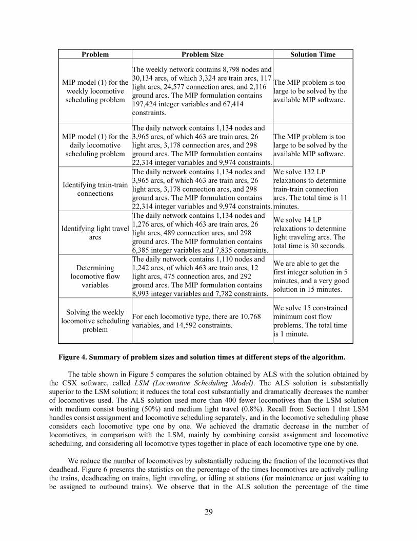
29

Problem Problem Size Solution Time

MIP model (1) for theweekly locomotivescheduling problem

The weekly network contains 8,798 nodes and30,134 arcs, of which 3,324 are train arcs, 117light arcs, 24,577 connection arcs, and 2,116ground arcs. The MIP formulation contains197,424 integer variables and 67,414constraints.

The MIP problem is toolarge to be solved by theavailable MIP software.

MIP model (1) for thedaily locomotive

scheduling problem

The daily network contains 1,134 nodes and3,965 arcs, of which 463 are train arcs, 26light arcs, 3,178 connection arcs, and 298ground arcs. The MIP formulation contains22,314 integer variables and 9,974 constraints.

The MIP problem is toolarge to be solved by theavailable MIP software.

Identifying train-trainconnections

The daily network contains 1,134 nodes and3,965 arcs, of which 463 are train arcs, 26light arcs, 3,178 connection arcs, and 298ground arcs. The MIP formulation contains22,314 integer variables and 9,974 constraints.

We solve 132 LPrelaxations to determinetrain-train connectionarcs. The total time is 11minutes.

Identifying light travelarcs

The daily network contains 1,134 nodes and1,276 arcs, of which 463 are train arcs, 26light arcs, 489 connection arcs, and 298ground arcs. The MIP formulation contains6,385 integer variables and 7,835 constraints.

We solve 14 LPrelaxations to determinelight traveling arcs. Thetotal time is 30 seconds.

Determininglocomotive flow

variables

The daily network contains 1,110 nodes and1,242 arcs, of which 463 are train arcs, 12light arcs, 475 connection arcs, and 292ground arcs. The MIP formulation contains8,993 integer variables and 7,782 constraints.

We are able to get thefirst integer solution in 5minutes, and a very goodsolution in 15 minutes.

Solving the weeklylocomotive scheduling

problem

For each locomotive type, there are 10,768variables, and 14,592 constraints.

We solve 15 constrainedminimum cost flowproblems. The total timeis 1 minute.

Figure 4. Summary of problem sizes and solution times at different steps of the algorithm.

The table shown in Figure 5 compares the solution obtained by ALS with the solution obtained bythe CSX software, called LSM (Locomotive Scheduling Model). The ALS solution is substantiallysuperior to the LSM solution; it reduces the total cost substantially and dramatically decreases the numberof locomotives used. The ALS solution used more than 400 fewer locomotives than the LSM solutionwith medium consist busting (50%) and medium light travel (0.8%). Recall from Section 1 that LSMhandles consist assignment and locomotive scheduling separately, and in the locomotive scheduling phaseconsiders each locomotive type one by one. We achieved the dramatic decrease in the number oflocomotives, in comparison with the LSM, mainly by combining consist assignment and locomotivescheduling, and considering all locomotive types together in place of each locomotive type one by one.

We reduce the number of locomotives by substantially reducing the fraction of the locomotives thatdeadhead. Figure 6 presents the statistics on the percentage of the times locomotives are actively pullingthe trains, deadheading on trains, light traveling, or idling at stations (for maintenance or just waiting tobe assigned to outbound trains). We observe that in the ALS solution the percentage of the time

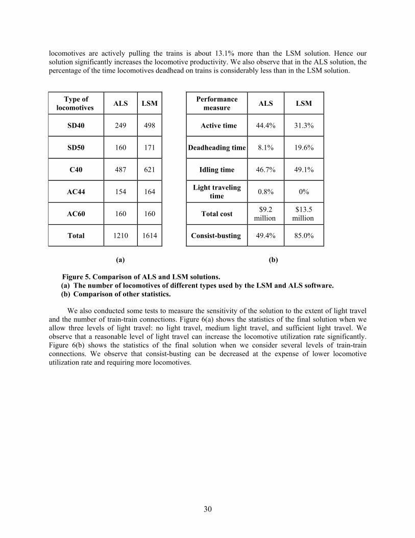
30

locomotives are actively pulling the trains is about 13.1% more than the LSM solution. Hence oursolution significantly increases the locomotive productivity. We also observe that in the ALS solution, thepercentage of the time locomotives deadhead on trains is considerably less than in the LSM solution.

Type oflocomotives ALS LSM Performance

measure ALS LSM

SD40 249 498 Active time 44.4% 31.3%

SD50 160 171 Deadheading time 8.1% 19.6%

C40 487 621 Idling time 46.7% 49.1%

AC44 154 164 Light travelingtime 0.8% 0%

AC60 160 160 Total cost $9.2million

$13.5million

Total 1210 1614 Consist-busting 49.4% 85.0%

(a) (b)

Figure 5. Comparison of ALS and LSM solutions.(a) The number of locomotives of different types used by the LSM and ALS software.(b) Comparison of other statistics.

We also conducted some tests to measure the sensitivity of the solution to the extent of light traveland the number of train-train connections. Figure 6(a) shows the statistics of the final solution when weallow three levels of light travel: no light travel, medium light travel, and sufficient light travel. Weobserve that a reasonable level of light travel can increase the locomotive utilization rate significantly.Figure 6(b) shows the statistics of the final solution when we consider several levels of train-trainconnections. We observe that consist-busting can be decreased at the expense of lower locomotiveutilization rate and requiring more locomotives.

31

ConsistBusting: 50%

No LightTravel

Medium lighttravel

Sufficientlight travel

Total numberof locomotives

used1268 1210 1192

Total cost $9,431,228 $9,242,092 $9,182,314 Percentageactive time 39.14% 44.44% 45.26%

Percentagedeadheading

time12.37% 8.09% 7.33%

Percentageidling time 48.49% 46.67% 46.06%

Percentagelight traveling

time0.00% 0.80% 1.35%

(a)

Very hight

consist-busting Hight consist-busting

Mediumconsist-busting Low consist-

busting

Minimumconsist-busting

Consist bustingrate 66.39% 59.48% 49.42% 39.09% 31.06%

Number oflocomotive

used1155 1165 1210 1281 1340

Total cost $9,052,779 $9,064,822 $9,242,092 $9,532,021 $9,772,958 Percentageactive time 46.68% 45.74% 44.44% 42.67% 41.25%

Percentagedeadheading

time6.28% 6.79% 8.09% 9.99% 9.57%

Percentageidling and

dwelling time46.23% 46.68% 46.67% 46.35% 48.04%

Percentagelight traveling

time0.81% 0.79% 0.80% 0.99% 1.14%

(b)

Figure 7. Sensitivity of the solution to light travel and consist-busting.

32

10. SUMMARY AND CONCLUSIONS

In this paper, we present the results of a study of a locomotive scheduling problem faced by CSXTransportation, a major US railroad company. We focused on the planning version of the locomotivescheduling problem, where we assign locomotive types to various trains. Our goal was to developexcellent plans along a number of dimensions. Our primary metric for evaluating a solution was tocompare it to the existing software used by the locomotive planning division at CSX. The existingsoftware was in-house software developed over a period of ten years. While it has the substantialadvantage of capturing many constraints and objectives not dealt with in the existing literature, it also hassome important limitations. In particular, it was unable to produce acceptable solutions withoutconsiderable manual adjustment of the solution produced. Our approach to solve the planning version ofthe locomotive scheduling problem produced solutions that satisfied the constraints and business rulesspecified by CSX and offered considerable savings in cost, especially in terms of a significant reductionin the number of locomotives needed. Our model is the first approach to account for consist busting, lighttravel, and consistency of the solution in a unified framework. Our approach relies upon breaking thelocomotive scheduling problem into a two-step process: first solving the daily locomotive schedulingproblem, and then solving the weekly locomotive scheduling problem. This approach works reasonablywell for those situations where a large number of trains run most days in a week.

By incorporating more realistic constraints and costs in our models, we needed to rely on amultistage heuristic procedure to solve the model. In particular, we were unable to solve MIPs involvingmany fixed charge constraints. We avoided this with a sequential heuristic procedure for determining thethree sets of decision variables (i) light travel, (ii) train-train connections, and (iii) active and deadheadlocomotive flow variables sequentially instead of determining them in a single model. Nevertheless, oursequential procedure heavily exploited information from a sequence of LPs, and thus relied on a systemwide view of the entire planning problem. When we determine light travel arcs, we consider locomotiveflow variables are also part of the LPs solved. Similarly, when we determine train-train connectionvariables, we again consider locomotive flow variables in the decision process. Hence we do achieve acertain level of integration in our sequential approach. Perhaps in the future we will be able to obtain abetter integration of these different sets of variables.

From the CSX perspective, this research demonstrated that advances in OR techniques enabled asimultaneous locomotive assignment and scheduling solution on a much larger network than previouslythought possible. CSX used the model in support of its operations planning effort associated with itsacquisition of Conrail territory, a 30% increase in network size. Without the aid of the model, CSX wouldnot have been confident in its ability to execute the new integrated operating plan. In addition, CSXexecuted a major locomotive trade with a locomotive leasing company where they swapped 156 older,low and medium horsepower locomotives for 31 newer, high horsepower locomotives. The model helpedquantify the network benefits of re-centering the fleet composition. In the future, CSX is interested inexpanding on this work to include locomotive fueling and servicing constraints into the algorithm. CSXalso intends to introduce decision support tools into its tactical management process.

ACKNOWLEDGEMENTS:

We would like to acknowledge the help of our students, Anurag Chandra (MIT) , Ozlem Ergun(MIT), Anurag Mehta (University of Florida), and Mukundhan Krishnaswamy (University of Delaware),who participated in this project and contributed in different capacities. The project was mainly funded byCSX Transportation and we gratefully appreciate the help the CSX Locomotive Division for giving us theresearch grant and access to their data. The project was also partly funded by the National ScienceFoundation Grants # DMI-9900087, DMI-0085682, DMI-9820998 and the Office of Naval ResearchGrant ONR N00014-98-1-0317 to the first and third coauthors.

33

REFERENCES:

Aarts, E. H. L., and J. K. Lenstra, J. K. (editors). 1997. Local search in Combinatorial Optimization. JohnWiley & Sons, New York, NY.

Ahuja, R. K., T.L. Magnanti, and J.B. Orlin. 1993. Network Flows: Theory, Algorithms, and Applications.Prentice Hall, NJ.

Ahuja, R. K., O. Ergun, J. B. Orlin, and A.P. Punnen. 2002. A survey of very large scale neighborhoodsearch techniques. To appear in Discrete Applied Mathematics.

Ahuja, R. K., J. B. Orlin, and D. Sharma. 2001a. Multi-exchange neighborhood search algorithms for thecapacitated minimum spanning tree problem. Mathematical Programming 91, 71-97.

Ahuja, R. K., J. B. Orlin, and D. Sharma. 2001b. A composite very large-scale neighborhood structure forthe capacitated minimum spanning tree problem. Submitted to Operations Research Letters.

Ahuja, R. K., J. B. Orlin, and D. Sharma. 2001c. A very large-scale neighborhood search algorithm forthe combined through-fleet assignment model. Submitted to INFORMS Journal on Computing.

Barnhart, C., N.L. Boland, L.W. Clarke, E.L. Johnson, G.L. Nemhauser, and R. Shenoi. 1998. Flightstring models for aircraft fleeting and routing. Transportation Science 32, 208-219.

Brannlund, U., P. O. Lindberg, A. Nou, and J. -E. Nilsson. 1998. Railway timetabling using Lagrangianrelaxation. Transportation Science 32, 358-369

Chih, K.C., M.A. Hornung, M.S. Rothenberg, and A.L. Kornhauser. 1990. Implementation of a real timelocomotive distribution system. In Computer Applications in Railway Planning and Management,T. K. S. Murthy, R. E. Rivier, G. F. List and J. Mikolaj (eds.) Computational MechanicsPublications, Southampton, U.K., 39-49.

Cordeau, J.-F., P. Toth, and D. Vigo. 1998. A survey of optimization models for train routing andscheduling. Transportation Science 32, 988-1005.

Fischetti, M. and P. Toth. 1997. A package for locomotive scheduling, Technical Report DEIS-OR-97-16,University of Bologna, Italy.

Florian, M. G. Bushell, J. Ferland, G. Guerin, and L. Nastansky. 1976. The engine scheduling problem ina railway network. INFOR 14, 121-138.

Forbes, M.A., J.N. Holt, and A.M. Watts. 1991. Exact solution of locomotive scheduling problems.Journal of Operational Research Society 42, 825-831.

Glover, F., and M. Laguna. 1997. Tabu Search. Kluwer Academic Publishers, Norwell, MA.

Goldberg, A.V. 1995. Scaling algorithms for the shortest path problem. SIAM Journal on Computing 24,494-504.

Hane, C. A., C. Barnhart, E.L. Johnson, R.E. Marsten, G.L. Nemhauser, and G. Sigmondi. 1995. The fleetassignment problem: Solving a large-scale integer program. Mathematical Programming 70, 211-232.

Jovanovic, D. and P. T. Harker. 1991. A decision support system for train dispatching: An optimization-based methodology, Transportation Research Record 1314, 31-40.

Mao, C-K., and C. D. Martland. 1981. Utilization of railroad motive power: Train delay impacts andorganizational considerations. The Logistics and Transportation Review 17, 291-312.

34

Newton, H. N., C Barnhart, and P. H. Vance. 1998. Constructing railroad blocking plans to minimizehandling costs. Transportation Science 32, 330-345.

Nou, A., J. Desrosiers, and F. Soumis. 1997. Weekly locomotive scheduling at Swedish State Railways,Technical report G-97-35, GERAD, Ecole des Hautes Etudes Commercials de Montreal, Canada.

Smith, S. and Y. Sheffi. 1988. Locomotive scheduling under uncertain demand. Transportation ResearchRecord 1251, 45-53.

Sherali, H. D., and A. B. Suharko. 1988 A tactical decision support system for empty railcar management.Transportation Science 32, 306-329.

Subramanium, R., R. P. Scheff Jr., J. D. Quillinan, D. S. Wiper, and R. E. Marsten. 1994. Coldstart: Fleetassignment at Delta Air Lines. Interfaces 24, 104-120.

Ziarati, K., F. Soumis, J. Desrosiers, S. Gelinas, and A. Saintonge. 1997. Locomotive assignment withheterogeneous consists at CN North America. European Journal of Operational Research 97, 281-292.

Ziarati, K., F. Soumis, J. Desrosiers, and M. M. Solomon. 1999. A branch-first, cut-second approach forlocomotive assignment, Management Science 45, 1156-1168.