arX

iv:c

ond-

mat

/010

9377

v1 [

cond

-mat

.sta

t-m

ech]

20

Sep

2001

Solvable model for electrolytic soap films:

the two-dimensional two-component plasma

Gabriel Tellez∗ and Lina Merchan†

Departamento de Fısica, Universidad de Los Andes, A.A. 4976, Bogota, Colombia

We study a toy model for electrolytic soap films, the two-dimensional two-component plasma.This model is exactly solvable for a special value of the coulombic coupling constant βq2 = 2. Thisallows us to compute the disjoining pressure of a film and to study its stability. We found that theCoulomb interaction plays an important role in this stability. Also the adhesivity that measures theattraction of soap anions to the boundaries is very important. For large adhesivity the film is stable,whereas for small adhesivity a collapse could occur. We also study the density and correlations inthe film. The charge density near the boundary shows a double layered profile. We show that thecharge correlations verify a certain number of sum rules.

PACS numbers: 5.20.Jj, 68.15.+e, 61.20.Qg, 05.70.Np

Keywords: soap films, Coulomb systems, disjoining pressure, charge density, correlations

I. INTRODUCTION

When soap molecules interact with water they disso-ciate into anions and cations. The soap anions havea hydrophilic head and a hydrophobic tail. Therefore,their negative tails prefer to lie on the surface of the filmwhile the positive ions can remain throughout the film.Soap films have a simple configuration and a well defineddouble layered structure, hence constituting an excellentsystem to be modeled by a Coulomb gas in a confinedgeometry. We are interested in the Coulomb interactionbetween the ions of a two-dimensional soap film and howit contributes to the collapse to a black film.

A soap film, when subject to certain circumstances,may collapse to a thickness smaller than visible light wavelength and therefore it is seen black. This phenomenonwas observed in the experiments held by O. Belorgey andJ. J. Benattar [1] and later by D. Sentenac and J. J. Be-nattar [2]. In both cases, salt was added to the soapsolution. Depending on both the salt concentration andtemperature, if the external pressure was increased to acertain point the soap film collapsed to either a CommonBlack Film (CBF) or to a Newton Black Film (NBF). Ac-cording to O. Belorgey and J. J. Benattar [1], the CBFequilibrium thickness is due to a balance among attrac-tive van der Waals forces and repulsive forces betweenthe layers. It is believed that short range repulsive forcesassociated to the local structure of water are responsi-ble for the NBF stability. The sole difference betweenthese two kinds of black films is the thickness of the wa-ter layer. The CBF water layer is more than seven timesas thick as the NBF water layer. But the external lipidlayer has the same width in both black films. In spiteof this, the structure and forces involved in black filmsare not completely understood. We want to know if the

∗Electronic address: gtellez@uniandes.edu.co†Electronic address: l-mercha@uniandes.edu.co

coulombic forces play a role in this phenomenon.In 1997, the mean field Poisson-Boltzmann theory was

applied by Dean and Sentenac [3] to three-dimensionalsoap films. Within this framework, they studied the dis-joining pressure of the soap film for a wide range of saltconcentrations and widths of the film. This disjoiningpressure is the difference between the external and inter-nal pressures of the film. However, the phenomenon ofcollapse could not be explained by this mean field ap-proach. Later Dean, Horgan and Sentenac [4] used afunctional integral technique to examine a solvable one-dimensional Coulomb system model for a soap film. Theyfound the film charge distribution and discussed the sta-bility criterion for the one-dimensional film. In thatmodel they observed the collapse of the film, so one oftheir conclusions was that electrostatic forces play an im-portant role in this phenomenon.

In order to see what aspects are particular to the one-dimensional model and what aspects are more general westudy here another type of solvable model for a Coulombsystem that can be applied to soap films. Working inthe framework of classical statistical mechanics, we willmodel the soap film as a symmetric two-dimensional two-component plasma, i.e, a neutral system of positive andnegative particles of opposite charges ±q embedded ina neutral background. We are only interested in therole that the Coulomb interaction plays in the collapse ofthe film so forces like van der Waals and others will notbe considered. We will only consider salt-free systems.Also, the internal structure of the particles will not beregarded. This model is exactly solvable for a tempera-ture given by q2/kBT = 2. The attraction of the anionsto the interfaces will be accounted for by a short rangeattractive potential. We will study a film that has aninfinite surface and a finite thickness. The two dimen-sions to be considered lie on the breadth of the film, sothis system is invariant in one of the two dimensions. Wewill study separately the inner and outer regions of thefilm. For this reason we will use two models. Each oneis meant to be used to analyze one of the two regions.

The outline of this paper is as follows. First, in Sec. II

2

we will describe the two models we employ. Then, thereis brief explanation of the two-component plasma theoryand of the general method of solution. In Sec. III, we usethe technique presented in Sec. II to find the pressureinside the film. Afterward, in Sec. IV, we will show howto compute the one-particle densities and the truncatedtwo-body densities. Each calculation is followed by itscorresponding analysis. Finally, we conclude on the rolethat electrostatic forces play in the collapse of this two-dimensional soap film.

The main interest of our work is to study a solvablemodel for a soap film. Given the limitations of this two-dimensional model, we can only compare qualitativelythe structure and behavior of this film to a real one.

II. THE MODEL AND METHOD OF

RESOLUTION

In this section, we will present the two models we em-ployed to study a two-dimensional soap film. The twomodels have a lot in common. Both are two dimensionalsystems of particles of charge ±q confined in a slab of im-penetrable walls. This aspect is modeled by an infiniteexternal potential outside the slab. The anions, nega-tively charged, tend to lie on the external surface of thefilm. This is accounted for by an attractive short rangepotential of different form in each model. The cations,on the other hand, can lie anywhere in the film and thisis represented by a constant potential. This potential isthe same in the two models.

In the first model (model I), the short range potentialis modeled by a delta function, while in model II, it ismodeled by a step function. The first model will be usedto find the pressure and the densities in the inner regionof the film whilst the second model will be employed inthe computation of the correlations and the densities inthe outer layers of the film.

In two dimensions, the Coulomb interaction potentialof a charge sq at a distance r from another charge s′q islogarithmic, of the form v(r) = −ss′q2 ln(r/d), where d isan irrelevant length scale. The adimensional coulombiccoupling constant is Γ = βq2. For a system of pointparticles the attraction between pairs of opposite signwill make the system unstable at low temperatures. Forthis reason the partition function is not well defined forΓ ≥ 2. While for Γ < 2, the system is stable againstcollapse.

Let us review the method described by Jancovici andCornu [5] for the two-component plasma. We start withthe grand partition function

Ξ =

∞∑

N=0

1

N !λN

0

∫

dr1

∫

dr2...

∫

drN exp (−βH) ,

(2.1)

where N is the number of particles and λ0 is the con-stant fugacity related to the kinetic energy and the

chemical potential. We consider only neutral config-urations: the number of positive particles is equal tothe number of negative particles. An external poten-tial can be described by a position dependent fugacityλ (ri) = λ0 exp (−βUext (ri)). In order to avoid diver-gences we start with a discretized model. The positionvector r = (x, y) will be represented by a complex numberz = x+iy. The particles lie in two interwoven sublatticesU and V . The positives particles reside in the sublatticeU with coordinates ui, while the negatively charged par-ticles reside in the sublattice V with coordinates vi.

For a specific temperature, given by q2/kBT = 2,this model is exactly solvable. For a configuration withN positive particles and N negative particles, using aCauchy identity, it can be shown that

exp

−β∑

i<j

v (rij)

= d2N

∣

∣

∣

∣

∣

[

det1

ui − vj

]

i,j=1,...,N

∣

∣

∣

∣

∣

2

.

(2.2)

Using this fact, the grand partition function can be writ-ten as

Ξ = det

∣

∣

∣

∣

∣

∣

∣

∣

∣

∣

∣

∣

∣

∣

∣

∣

∣

1 0 · · · d λ(u1)u1−v1

d λ(u1)u1−v2

· · ·0 1 · · · d λ(u2)

u2−v1

d λ(u2)u2−v2

· · ·...

.... . . · · · · · · · · ·

d λ(v1)v1−u1

d λ(v1)v1−u2

... 1 0 · · ·d λ(v2)v2−u1

d λ(v2)v2−u2

... 0 1...

......

...

∣

∣

∣

∣

∣

∣

∣

∣

∣

∣

∣

∣

∣

∣

∣

∣

∣

.

(2.3)

If each lattice site is characterized by a complex coor-dinate z and by a vector which is (1, 0) for the positiveparticles and (0, 1) for the negative particles then thegrand potential can be expressed in the following simpli-fied form

Ξ = det

[

1 +

(

λ+(r) 00 λ−(r)

) (

0 dz−z′

dz−z′

0

)]

. (2.4)

with λs the fugacity for particles of sign s.In the continuum limit where the lattice spacing goes

to zero (ignoring divergences for the time being) by usingthe identity

∂

∂z

1

z − z′=

∂

∂z

1

z − z′= πδ (r − r

′) , (2.5)

it can be shown that

Ξ = det

[

(

0 2∂z

2∂z 0

)−1 (

m+(r) 2∂z

2∂z m−(r)

)

]

, (2.6)

where ms = 2πdS λs are rescaled fugacities (S is the area

of a lattice site). Then defining a new matrix K as

K =

(

0 2∂z

2∂z 0

)−1 (

m+(r) 00 m−(r)

)

, (2.7)

3

the grand partition function Ξ can be expressed as

Ξ = det (1 +K) . (2.8)

The calculation of the pressure, p = −∂ω/∂W , reducesto finding the eigenvalues of K. While, on the otherhand, the calculation of the one-particle densities andcorrelations reduces to finding the Green functions G,satisfying the following set of equations

(

m+(r1) ∂x1− i∂y1

∂x1+ i∂y1

m−(r1)

)

G(r1, r2) = δ(r1 − r2)1 ,

(2.9)

where

G =

(

G++ G+−

G−+ G−−

)

, (2.10)

and 1 is the unit 2×2 matrix, since it can be shown that

ρs1(r1) = ms1

Gs1s1(r1, r1) , (2.11a)

ρ(2)Ts1s2

(r1, r2) = −ms1ms2

Gs1s2(r1, r2)Gs1s2

(r2, r1) .

(2.11b)

When an external potential is acting differently on posi-tive and negative particles, it is convenient to definem (r)and V (r) as

ms (r) = m (r) exp [−2sV (r)] . (2.12)

To symmetrize the problem for the two types of parti-cles, it is useful to define the following modified Greenfunctions

gs1s2(r1, r2) = e−s1V (r1)Gs1s2

(r1, r2) e−s2V (r2). (2.13)

Using the following operators

A = ∂x1+ i∂y1

+ ∂x1V (r1) + i∂y1

V (r1) , (2.14a)

A† = −∂x1+ i∂y1

+ ∂x1V (r1) − i∂y1

V (r1) , (2.14b)

the equations for g++ and g−− decouple into

{

m (r1) +A† [m (r1)]−1A

}

g++ (r1, r2) = δ (r1 − r2) ,

(2.15a)

{

m (r1) +A [m (r1)]−1A†

}

g−− (r1, r2) = δ (r1 − r2) .

(2.15b)

The other Green functions are given by

g−+ (r1, r2) = − [m (r1)]−1Ag++ (r1, r2) (2.16a)

g+− (r1, r2) = [m (r1)]−1A†g−− (r1, r2) . (2.16b)

We will apply the above method to the models explainednext.

The film has a thickness W . The outer region has awidth δ, while the inner region has a thickness 2L. Thebreadth of the film is in the x-axis and the film is infinitein the y-axis. The origin is set in the middle of the soapfilm. Remembering that ms ∝ exp (−βUext(r)), in modelI, the position dependent fugacities are

m+(r) = m, (2.17a)

m−(r) = m+ α(δ(x − L) + δ(x+ L)) . (2.17b)

The parameter α which we will call adhesivity mesuresthe strength of the attractive potential.

Model II differs from the preceding in that the attrac-tive potential acts over a region of length δ. For a realsoap film, this thickness is approximately the length ofthe hydrophobic tail. So for this model the position de-pendent fugacities are

m+(x) = m (2.18a)

m−(x) =

{

mi if x ∈ [−L− δ,−L[ ∪ ]L,L+ δ]

m if x ∈ [−L,L] .

(2.18b)

withmi = m exp(−βUext) > m since Uext is an attractiveconstant potential. We can therefore distinguish threeregions: the left border −L− δ < x < −L (region 1), thebulk of the film −L < x < L (region 2) and the rightborder L < x < L+ δ (region 3).

In this case, the Eqs. (2.15) and (2.16) simplify to[

(m(x1))2 − ∆

]

g±± (x1, x2, l) = m(x1)δ (x1 − x2)

(2.19a)

1

m(x1)[−∂x ∓ i∂y] g±± (x1, x2, l) = g∓± (x1, x2, l)

(2.19b)

where

m(x) =

{

m0 = (mmi)1/2 if x in regions 1 or 3 ,

m if x in region 2 .

(2.20)

In this model, the potential defined in Eq. (2.12) is thefollowing

exp (V ) =

{

(

mi

m

)1

4 if x in regions 1 or 3 ,

1 if x in region 2 .(2.21)

With this model we will study the case where mi → ∞and δ → 0 while keeping their product constant. Thisway model I is a limiting case of model II.

III. THE PRESSURE

A. Formal expression for the grand potential

We shall use here the first model presented in the abovesection (model I), where the position-dependent fugaci-

4

ties are given by Eqs. (2.17). As explained in the preced-ing section the grand potential is given by

Ξ = det(1 +K) , (3.1)

To compute the grand potential we need to find the eigen-values of K. The eigenvalue problem for K with eigen-values λ and eigenvectors (ψ, χ) reads

m−(r)χ(r) = 2λ∂zψ(r) , (3.2a)

m+(r)ψ(r) = 2λ∂zχ(r) . (3.2b)

From Eqs. (3.2) and (2.17) we find that χ is a continuousfunction while ψ(x, y) is discontinuous at x = ±L due tothe Dirac delta distributions in m−(r). The discontinuityof ψ is given by Eqs. (3.2a) and (2.17b)

ψ(x = ±L+, y) − ψ(x = ±L−, y) =α

λχ(x = ±L, y) .

(3.3)

Inside the film, for −L < x < L, Eqs. (3.2) can be com-bined into the Laplacian eigenvalue problem

∆χ =(m

λ

)2

χ . (3.4)

Due to the translational invariance in the y-direction welook for solutions of the form

χ(r) = (Ae−κ∗x +Beκ∗x)eiky , (3.5)

where κ∗ = (k2 + (m/λ)2)1/2. From Eq. (3.2b) we find

ψ(r) =λ

m(A(k − κ∗)e−κ∗x +B(κ∗ + k)eκ∗x)eiky .

(3.6)

Outside the film Eqs. (3.2) reduce to

∂zψ = 0 and ∂zχ = 0 . (3.7)

That is ψ is analytic and χ is antianalytic. Since we arelooking for solutions with y dependence eiky this gives

ψ(r) = Cekz = Cekx+iky , (3.8a)

χ(r) = De−kz = De−kx+iky . (3.8b)

In order to have vanishing solutions at infinity, from thepreceding equations it is necessary that for k > 0

ψ(r) = 0 for x > L , (3.9a)

χ(r) = 0 for x ≤ −L , (3.9b)

and for k < 0

ψ(r) = 0 for x < −L , (3.9c)

χ(r) = 0 for x ≥ L . (3.9d)

Eqs. (3.3) and (3.9) are the boundary conditions thatcomplete the Laplacian eigenvalue problem (3.4). Theseboundary conditions yield a homogeneous linear system

for the coefficients A and B, which in the case k > 0reads

(

A B)

(

(λ2(k − κ∗) + αm)e−κ∗L eκ∗L

(λ2(κ∗ + k) + αm)eκ∗L e−κ∗L

)

= 0 .

(3.10)

In order to have non trivial solutions the determinant ofthis linear system must vanish. This gives the followingequation that must be satisfied by the eigenvalues λ

(λ2(κ∗ + k) + αm)e2κ∗L + (λ2(κ∗ − k) − αm)e−2κ∗L = 0 ,(3.11)

that can also be written as

cosh(2κ∗L) +(

k +αm

λ2

)

sinh(2κ∗L)/κ∗ = 0 . (3.12)

A similar equation is found for the case k < 0 in whichone should change k for −k. As a consequence of this factthe set of solutions for k < 0 is the same as for k > 0.From now on we will only consider the case k > 0.

The grand potential per unit length is then given by

βω = − 1

2π

∫ +∞

−∞

ln∏

λk

(1 + λk) dk

= − 1

π

∫ +∞

0

ln∏

λk

(1 + λk) dk , (3.13)

where the product runs over all λk solution of Eq. (3.12).This product can actually be performed as explained inrefs. [6, 7, 8]. Let us introduce the analytic function

fk(z) = cosh(2√

k2 +m2z2L)

+(

k + αmz2) sinh(2

√k2 +m2z2L)√

k2 +m2z2.(3.14)

By construction the zeros of fk are the inverse of theeigenvalues λk. This function fk can be factorized as aWeierstrass product running over its zeros. Since fz(0) =exp(2kL), f ′(0) = 0, f(z) = f(−z) and the zeros of fk

are 1/λk, the Weierstrass product representation reducesto

fk(z) = exp(2kL)∏

λk

(1 − zλk) . (3.15)

Then the product appearing in the grand potential (3.13)is simply fk(−1)e−2kL. Finally, the grand potential perunit length reads

βω = − 1

π

∫ ∞

0

dk

[

− 2kL+ (3.16)

+ ln

(

cosh(2κL) +k + αm

κsinh(2κL)

)]

,

where κ = (k2 +m2)1/2. The above integral is actuallydivergent and should be cutoff to a kmax ≃ 1/R where R

5

is the diameter of the particles as explained in Ref. [5].It can be checked that for α = 0, Eq. (3.16) yields theknown grand potential for a two-component plasma in astrip of hard walls [6].

It is interesting to look at the large-L behavior of thegrand potential,

ω = −Wpb + 2γ +O(

e−mW)

, (3.17)

where W = 2L is the width of the film, the bulk pressureis given by

βpb =1

π

∫ 1/R

0

(κ− k) dk

=m2

2π

(

ln2

mR+ 1

)

, (3.18)

(a known result from Refs. [5, 6], in the limit of vanishingcutoff R → 0), and the surface grand potential is

βγ = − 1

2π

∫ 1/R

0

ln

[

1

2

(

1 +k +mα

κ

)]

dk . (3.19)

In the limit R → 0 the surface grand potential reads

βγ = −m

4π

[

α ln2

mR+ 1 − π + α+

1 − α2

αln(α + 1)

]

.

(3.20)

When α = 0 the above expression reduces to the knownresult [6, 9]

βγ(α = 0) =m

2π

(π

2− 1

)

. (3.21)

When the cutoff R vanishes the surface grand potentialdiverges (except for α = 0). This is expected since neg-ative particles are strongly attracted to the boundariesand for point particles this would create divergences inthe surface grand potential in addition to the usual diver-gences in the bulk pressure due to the collapse of particlesof opposite sign.

Finally it should be noted in Eq. (3.17) that there areno algebraic corrections in 1/W to the grand potential.The next correction after the surface term is exponen-tially small. This is the same situation as in a strip withhard walls (α = 0) but very different from the situa-tion of ideal conducting boundaries [6] and ideal dielec-tric boundaries [10]. In those later cases there is indeedan algebraic universal finite-size correction to the grandpotential equal to π/24W .

B. The disjoining pressure

The pressure in the film can be obtained from thegrand potential as p = −∂ω/∂W . The disjoining pres-sure is defined as the difference between the pressure ofthe film and the pressure of an infinite system (W → ∞,

FIG. 1: The disjoining pressure pd as a function of thewidth W for several values of α. From top to bottomα = 2, 1, 0.5, 0.3, 0. Notice that the disjoining pressure be-comes positive for small W except in the case α = 0 where itis always negative.

the bulk pressure): pd = p− pb [4]. Using Eq. (3.16) forthe grand potential and Eq. (3.18) for the bulk pressure,we find

βpd =1

π

∫ ∞

0

g(k) dk , (3.22a)

with

g(k) =2κ(−κ+ k +mα)e−2κW

κ+ k +mα+ (κ− k −mα)e−2κW. (3.22b)

In the limit W → 0, the total pressure is

βp(W = 0) =mα

πR. (3.23)

For W = 0 and α 6= 0, the pressure diverges as 1/R whenthe cutoff vanishes, stronger than the usual logarithmicdivergence. From this fact, it is clear that for α 6= 0 thedisjoining pressure will be positive whenW → 0 (actuallypd → +∞ as W → 0). The case α = 0 is particular sincethen the disjoining pressure is of same order as minusthe bulk pressure for small-W and then pd → −∞ whenW → 0.

For non-zero width films W 6= 0 the disjoining pressureis finite for vanishing cutoff R→ 0 (this limit has alreadybeen taken in Eq. (3.22)).

Fig. (1) shows several plots of the disjoining pressure asa function of the width W , for different values of α. Wenotice two different behaviors. For α = 1 and α = 2, thepressure is a monotonous decaying function of the width.This indicates that the film is stable for all widths. Forα = 0.3 and α = 0.5, we notice that the pressure is nolonger a monotonous function of the width. There existsa “critical” width Wc and for W > Wc the pressure isan increasing function of the width. This indicates thatthe film is unstable for W > Wc. Indeed, in that regiona small change in the applied pressure to the film willresult into a collapse to a width smaller than the criticalWc. This transition is discontinuous (first order). This

6

FIG. 2: The disjoining pressure pd as a function of the widthW for α = 0.3. The critical length is Wc. The phenomenon ofcollapse is illustrated as follows. Initially the film has a widthWA corresponding to the point A in the pd – W diagram. Asmall change in the pressure will force the system to go topoint B: the film has collapsed to a width WB < Wc < WA.This transition is clearly first order (discontinuous).

is illustrated in Fig. (2). In the case α = 0 the disjoiningpressure is always negative and increases if W increases.The film is unstable for all widths when α = 0.

The critical value of α distinguishing between these twodifferent behaviors is αc = 1 as it will be shown below.In order to determine if the pressure is an increasing ordecreasing function of W we study the sign of ∂pd/∂Wand in particular the sign of ∂g(k)/∂W . We have

∂g(k)

∂W=

mκ2[

m(1 − α2) − 2αk]

e−2κW

[κ+ k +mα+ (κ− k −mα)e−2κW ]2 . (3.24)

Clearly for α ≥ 1 the function ∂g(k)/∂W is negativefor all values of k > 0, and consequently the disjoiningpressure will be a decreasing function of W .

For α < 1 the function ∂g(k)/∂W is positive for valuesof k < k∗ = m(1−α2)/2α and negative for values of k >k∗. Since for large values of W , the function ∂g(k)/∂Wdecays exponentially, the dominant part of the integralin

∂βpd

∂W=

1

π

∫ ∞

0

∂g(k)

∂Wdk , (3.25)

will be given by small values of k, where ∂g(k)/∂W ispositive. Then, for large values of W , ∂pd/∂W will bepositive and pd will be an increasing function of W forlarge W .

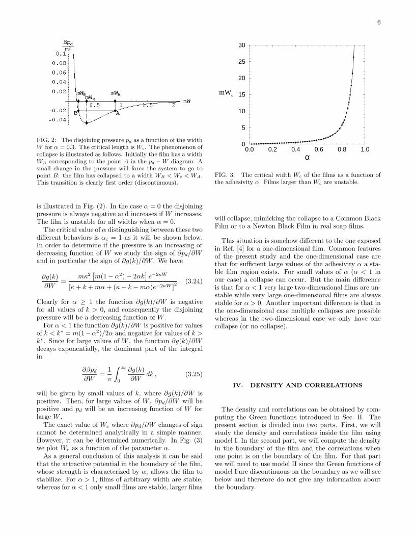
The exact value of Wc where ∂pd/∂W changes of signcannot be determined analytically in a simple manner.However, it can be determined numerically. In Fig. (3)we plot Wc as a function of the parameter α.

As a general conclusion of this analysis it can be saidthat the attractive potential in the boundary of the film,whose strength is characterized by α, allows the film tostabilize. For α > 1, films of arbitrary width are stable,whereas for α < 1 only small films are stable, larger films

0.0 0.2 0.4 0.6 0.8 1.0α

0

5

10

15

20

25

30

mWc

FIG. 3: The critical width Wc of the films as a function ofthe adhesivity α. Films larger than Wc are unstable.

will collapse, mimicking the collapse to a Common BlackFilm or to a Newton Black Film in real soap films.

This situation is somehow different to the one exposedin Ref. [4] for a one-dimensional film. Common featuresof the present study and the one-dimensional case arethat for sufficient large values of the adhesivity α a sta-ble film region exists. For small values of α (α < 1 inour case) a collapse can occur. But the main differenceis that for α < 1 very large two-dimensional films are un-stable while very large one-dimensional films are alwaysstable for α > 0. Another important difference is that inthe one-dimensional case multiple collapses are possiblewhereas in the two-dimensional case we only have onecollapse (or no collapse).

IV. DENSITY AND CORRELATIONS

The density and correlations can be obtained by com-puting the Green functions introduced in Sec. II. Thepresent section is divided into two parts. First, we willstudy the density and correlations inside the film usingmodel I. In the second part, we will compute the densityin the boundary of the film and the correlations whenone point is on the boundary of the film. For that partwe will need to use model II since the Green functions ofmodel I are discontinuous on the boundary as we will seebelow and therefore do not give any information aboutthe boundary.

7

A. Inside the film

1. The Green functions

In the present geometry it is natural to work with theFourier transform Gss′ of Gss′ in the y-direction

Gss′ (r1, r2) =

∫ ∞

−∞

Gss′ (x1, x2, k) eik(y1−y2)

dk

2π. (4.1)

Then Eq. (2.9) translates in Fourier space to

(

m+(x1) ∂x1+ k

∂x1− k m−(x1)

)

G(x1, x2, k) = δ(x1 − x2)1 .

(4.2)

Let us detail the calculation of G−− and G+−, the onefor G++ and G−+ follows similar steps. The equationsare

mG+− + (∂x1+ k)G−− = 0 , (4.3a)

(∂x1− k)G+− +m−(x1)G−− = δ(x1 − x2).(4.3b)

From Eq. (4.3a) we deduce that G−− is continuous. How-ever because of the Dirac delta distributions in the defi-nition of m− the function G+− will be discontinuous atx1 = ±L. From Eq. (4.3b) we deduce the discontinuity

of G+− at x1 = ±L if x2 6= x1

G+−(x1 = ±L−) − G+−(x1 = ±L+) = αG−−(x1 = ±L) ,(4.4)

If both points r1 and r2 are inside the film but not onthe boundary both fugacities are equal m+ = m− = m

and then Eqs. (4.3) can be combined into

(∂2x1

− κ2)G−−(x1, x2) = −mδ(x1 − x2) , (4.5)

with κ = (k2 +m2)1/2, while G+− is given by Eq. (4.3a).

If r1 is outside the film while r2 is fixed inside the film,thenm+(x1) = m−(x1) = 0 and the solution of Eqs. (4.3)is

G−−(x1, x2, k) = Ce−kx1 , (4.6a)

G+−(x1, x2, k) = Dekx1 . (4.6b)

In order to have finite solutions at x1 = ±∞ it is neces-sary that for k > 0

G−−(x1 ≤ −L) = 0 and G+−(x1 > L) = 0 ,(4.7a)

and for k < 0

G−−(x1 ≥ L) = 0 and G+−(x1 < −L) = 0 .(4.7b)

Eqs. (4.4) and (4.7) are the boundary conditions thatcomplement the differential equations (4.3) for the Greenfunctions.

The solution is of the form

G−−(x1, x2) =m

2κ

[

e−κ|x1−x2| + (4.8)

+Ae−κx1 +Beκx2

]

,

where the coefficients A and B are determined by theboundary conditions. Finally the Green function G−−

is, for k > 0,

G−−(x1, x2, k) =m

2κ

[

e−κ|x1−x2| +

+−(k + κ+ αm)e−κ(x1+x2) + (κ− k − αm)eκ(x1+x2)

(κ− k − αm)e−κW + (k + κ+ αm)eκW+

+2(−κ+ k + αm)e−κW coshκ(x1 − x2)

(κ− k − αm)e−κW + (k + κ+ αm)eκW

]

, (4.9a)

and for k < 0,

G−−(x1, x2, k) =m

2κ

[

e−κ|x1−x2| +

+(κ+ k − αm)e−κ(x1+x2) + (−κ+ k − αm)eκ(x1+x2)

(κ+ k − αm)e−κW + (κ− k + αm)eκW+

+2(−κ− k + αm)e−κW coshκ(x1 − x2)

(κ+ k − αm)e−κW + (κ− k + αm)eκW

]

, (4.9b)

8

and G+− can be obtained from Eq. (4.3a). Similar calculations lead to G++ for k > 0,

G++(x1, x2, k) =m

2κ

[

e−κ|x1−x2| +

+−(κ+ k)

(

1 − ακ+km

)

eκ(x1+x2) + (κ− k)(

1 + ακ−km

)

e−κ(x1+x2)

(κ− k − αm)e−κW + (κ+ k + αm)eκW+

+2(k − κ+ αm)e−κW coshκ(x1 − x2)

(κ− k − αm)e−κW + (κ+ k + αm)eκW

]

, (4.10a)

while for k < 0,

G++(x1, x2, k) =m

2κ

[

e−κ|x1−x2| +

+(κ+ k)

(

1 + ακ+km

)

eκ(x1+x2) − (κ− k)(

1 − ακ−km

)

e−κ(x1+x2)

(κ+ k − αm)e−κW + (κ− k + αm)eκW

+2(−k − κ+ αm)e−κW coshκ(x1 − x2)

(κ+ k − αm)e−κW + (κ− k + αm)eκW

]

. (4.10b)

The Green function G−+ is obtained from

G−+(x1, x2) = − 1

m(∂x1

− k)G++(x1, x2) . (4.11)

We omit the details of the calculation for G++. Let us

only note that in this case, G+− is continuous while G++

is discontinuous at x1 = ±L with

G++(x1 = ±L−) − G++(x1 = ±L+) = αG+−(x1 = ±L) .(4.12)

The Green functions G(r1, r2) in position space aregiven by the Fourier transform formula (4.1). The term

m exp(−κ|x1−x2|)/(2κ) that appears in all Gss give thebulk contribution to Gss [5]

Gbulk =m

2πK0(m|r1 − r2|) , (4.13)

where K0 is the modified Bessel function of the secondkind of order 0.

For α = 0 the expressions for the Green functions re-duce to known results [11].

2. The density

The density of species of charge s is given by

ρs(r) = ms(r)Gss(r, r) . (4.14)

Using Eqs. (4.9) and (4.10) for the Green functions weobtain the densities

ρ−(x) = ρb +m2

π

∫ ∞

0

(k − κ+ αm)e−κW − (k + αm) cosh(2κx)

(κ− k − αm)e−κW + (κ+ k + αm)eκW

dk

κ(4.15a)

ρ+(x) = ρb +m2

π

∫ ∞

0

(k − κ+ αm)e−κW −(

k − αm− 2αk2

m

)

cosh(2κx)

(κ− k − αm)e−κW + (κ+ k + αm)eκW

dk

κ(4.15b)

where ρb is the bulk density (actually divergent whenthe cutoff R → 0). The charge density ρ = ρ+ − ρ−

(measured in units of q) is then

ρ(x) =2mα

π

∫ ∞

0

κe−κW cosh(2κx) dk

κ+ k + αm+ (κ− k − αm)e−2κW.

(4.16)

9

FIG. 4: The charge density as a function of the position xfor several values of α. The width of the film is W = 8/m.From top to bottom α = 2, 1, 0.5, 0.3.

Fig. (4) shows several plots of the charge density as afunction of the position x. This figure can be understoodas follows. Because of the strong attractive potential onthe boundary an important part of the negative particles(the soap molecules) are stuck in the borders of the filmat x = ±L creating a layer of negative surface charge den-sity (actually it is really a linear charge density since oursystem is two-dimensional, in a three-dimensional case itwould be a real surface charge density). In the frameworkof model I, this negative surface charge density cannot beseen in Fig. (4) nor in the analytic expressions found forthe densities, but it will be studied in detail in the sec-ond part of this section (section IVB) when we will workmodel II.

The system on the interior of the film is then non-neutral with an excess positive charge. This excess pos-itive charge screens the negative surface charge densityat the borders as it can be seen on Fig. (4). The den-sity near the boundary is positive and becomes very largewhen the boundary is approached. Away from the bor-ders, near the middle of the film, the system is almostneutral. Also in Fig. (4) and from the analytic expres-sion (4.16) for the density it can be checked that thescreening length is of order m−1, a well-known result [5].It should be noted that for α = 0.3 and α = 0.5 thesystem should collapse according to the analysis of thepreceding section (Sec. III). However there is no hint onthe charge density profiles indicating the collapse. Thiswas also the case on the one-dimensional model [4].

The surface charge on one border −σ can be computedby using the screening sum rule

σ =

∫ L

0

ρ(x) dx , (4.17)

giving

σ =αm

2π

∫ ∞

0

(1 − e−2κW ) dk

κ+ k + αm+ (κ− k − αm)e−2κW.

(4.18)

Actually the above expression is divergent and shouldbe cutoff to a kmax ≃ 1/R as it has been done for thepressure. In section IVB a more direct calculation of σwill be done and the validity of the screening sum rulewill be proven.

The surface charge density σ is an increasing functionof W . Actually for large films it converges exponentiallyfast to the value

σb =αm

2π

∫ 1/R

0

1

κ+ k + αmdk

=m

4π

[

α ln2

mR− α2 + 1

αln(α+ 1) + 1

]

.(4.19)

The vanishing terms when R → 0 have been omitted inthe second equality. The dominant term of σb, when thecutoff vanishes, is proportional to α. It is clear that αcontrols how much the boundaries get charged.

For very large films W → ∞, it is interesting to studythe relationship between the surface charge density σb

and the surface tension. Actually the surface grand po-tential γ computed in Sec. III is really the surface tensionof the system since we are dealing with polarizable inter-faces [5, 12]. This is clear in model II (model I beinga special limit of model II) where the particles are freeto go from region −L < x < L to the boundary re-gions −L − δ < x < −L and L < x < L + δ. In thatmodel the control parameter for charging the boundariesis the attractive potential Uext, or equivalently the fugac-ity mi. For model I the control parameter is the adhe-sivity α. From the formal expressions of γ and σb givenby Eqs. (3.19) and (4.19) it can be verified that

σb = −βα∂γ∂α

, (4.20)

which can be regarded as a particular form of Lippmannequation for this model [5].

3. The correlations

The truncated two-body correlation function for a par-ticle of sign s at r1 and a particle of sign s′ at r2 is givenin terms of the Green functions by

ρ(2)Tss′ (r1, r2) = −ms(r1)ms′(r2)Gss′ (r1, r2)Gs′s(r2, r1) .

(4.21)

With the expressions for the Green functions given byEqs. (4.9) and (4.10) the correlation functions can beobtained.

Due to the screening properties the structure near aboundary will not be modified considerably by the pres-ence of the other boundary. For this reason it is inter-esting to study in further detail the case of large filmsW → ∞. The corrections for finite films are exponen-tially small in mW .

10

For W → ∞, taking the origin at the boundary (xis now changed to x + L), the Fourier transforms of theGreen functions simplify, for k > 0, to

G−−(x1, x2) = Gbulk −m

2κe−κ(x1+x2) , (4.22a)

G++(x1, x2) = Gbulk + (4.22b)

+m

2κ

(κ− k)[

1 + αm (κ− k)

]

κ+ k + αme−κ(x1+x2),

and for k < 0

G−−(x1, x2) = Gbulk + (4.22c)

+m

2κ

κ+ k − αm

κ− k + αme−κ(x1+x2) ,

G++(x1, x2) = Gbulk + (4.22d)

+m

2κ

(k − κ)[

1 − αm (κ− k)

]

κ− k + αme−κ(x1+x2).

As a very curious fact it should be noted that the pre-ceding expressions for G−− are formally identical withthe ones of Ref. [5] for a two-component plasma neara charged hard wall if one chooses in the later casethe external surface charge density of the wall equal to−αm/(2π). This does not mean that in our case thecharge density (which is actually not external to the sys-tem, but internal and due to the reorganization of chargesin the film) is −αm/(2π). In the preceding subsectionwe have computed the surface charge density −σ and weknow that it is not equal to −αm/(2π). Furthermore for

the Green functions G++ this comparison does not hold,

the expression for G++ given by Eqs. (4.22) and thosefrom Ref. [5] are very different.

It is clear from Eqs. (4.22) that the correlation func-tions will decay exponentially fast in the x-direction(through the width of the film). However it is well knownthat in the y-direction, parallel to the boundary, the cor-relation functions usually decay algebraically [13, 14, 15].For two-dimensional Coulomb systems, near a hard ordielectric (non-conducting) wall, they should decay asy−2. For a hard wall (α = 0) the total charge correla-

tion function S(r1, r2) = ρ(2)T++ (r1, r2) + ρ

(2)T−− (r1, r2) −

ρ(2)T−+ (r1, r2) − ρ

(2)T+− (r1, r2) should behave, for y = y1 −

y2 → ∞, as [13, 14, 15]

S(r1, r2) ≃f(x1, x2)

|y|2 , (4.23)

and the function f(x1, x2) should obey the sum rule

∫ ∞

0

dx2

∫ ∞

0

dx1 f(x1, x2) = − 1

2π2β. (4.24)

The preceding asymptotic behavior is very general for aCoulomb system near a plane hard wall.

Returning to our case, the Fourier transform of theGreen functions have a discontinuity at k = 0 whichwill translate in position space into a decay as 1/y for

large y, then the correlation functions will indeed havea decay as 1/y2. More precisely, the large-y behav-ior of the charge correlation function is found to beS(r1, r2) ≃ f(x1, x2)/y

2 with the function f(x1, x2) givenby

f(x1, x2) = −m2e−2m(x1+x2)

(α + 1)2π2. (4.25)

This function obeys the sum rule

∫ ∞

0

dx2

∫ ∞

0

dx1 f(x1, x2) = − 1

2π2β(α+ 1)2. (4.26)

According to Ref. [13, 14, 15] for a Coulomb system neara plane hard wall with an external charge density on thewall the sum rule (4.24) is not modified. In our case,where the boundary is charged by a fraction of the par-ticles of the system, the sum rule is modified. Howeverin the sum rule (4.26) we only accounted for the correla-tions of particles in the fluid. As we will see in Sec. IVBthere are also correlations for particles that are absorbedin the boundary and when these are taken into accountthe sum rule (4.24) is verified.

It is also interesting to comment on the case α → ∞.It can be checked that in that limit Eqs. (4.22) reduce to

G−−(x1, x2) = Gbulk −m

2κe−κ(x1+x2) , (4.27a)

G++(x1, x2) = Gbulk + (4.27b)

+(κ− k)2

2mκe−κ(x1+x2) ,

for all values of k. Computing the inverse Fourier trans-forms gives

G−−(r1, r2) =m

2π[K0(mr12) −K0(mr

∗12)](4.27c)

G++(r1, r2) =m

2πK0(r12) + (4.27d)

+m

2πe−iφ∗

12K2(mr∗12) ,

where r12 = |r1 − r2| and r∗12 = |r1 − r∗2| with r

∗2 =

(−x2, y2) being the image of r2. The angle φ∗12 is theangle of the vector r1 − r

∗2 with respect to the x-axis.

It is clear that, when α→ ∞, the Green functions haveno longer an algebraic decay along the y-direction. Thedecay is now exponential in all directions and of the formexp(−mr12) and exp(−mr∗12).

B. On the boundary of the film

We are now interested in the structure of the film at theboundary. Model I cannot give directly any informationon the density or the correlations at the boundary sincesome of the Green functions are discontinuous there. We

11

shall use instead model II where the fugacities are givenby

m−(x) =

{

mi if x ∈ [−L− δ,−L[ ∪ ]L,L+ δ] ,

m if x ∈ [−L,L] ,

(4.28)

and m+(x) = m everywhere. Recall that we distinguishbetween three different regions: the left border −L− δ <x < −L (region 1), the bulk of the film −L < x < L(region 2) and the right border L < x < L+ δ (region 3).

1. The Green functions

It is useful to work with the modified Green functionsas explained in Sec. II. As before we will concentrate onthe computation of g−−, the one for g++ follows the samelines. We fix the source point r2 in region 1. Then, theGreen function obeys Helmoltz equation in the differentregions

(∆r1−m(x1)

2)g−−(r1, r2) = −m(x1)δ(r1 − r2) ,(4.29)

and

g+−(r1, r2) =1

m(x1)(−∂x1

+ i∂y1)g−−(r1, r2) , (4.30)

with the position dependent fugacity

m(x) =

{

m0 = (mmi)1/2 if x in regions 1 or 3 ,

m if x in region 2 .

(4.31)

Working with the Fourier transforms gss′ of gss′ we have,if r1 is in region 1,

g−−(x1, x2) =m0

κ0e−κ0|x1−x2| + (4.32a)

+A1e−κ0x1 +B1e

κ0x1 ,

if r1 is in region 2,

g−−(x1, x2) = A2e−κx1 +B2e

κx1 , (4.32b)

and if r1 is in region 3,

g−−(x1, x2) = A3e−κ0x1 +B3e

κ0x1 , (4.32c)

with κ0 = (m20 + k2)1/2. The coefficients Ai and Bi are

determined by the following boundary conditions: Gss′

should be continuous at x1 = ±L and at x1 = ±(L+ δ).

Furthermore, for k > 0, G−− = 0 if x1 ≤ −L − δ and

G+− = 0 if x1 ≥ L + δ. And for k < 0, G−− = 0

if x1 ≥ L + δ and G+− = 0 if x1 ≤ −L − δ. Theseboundary conditions yield a linear system of six equationsfor the coefficients Ai and Bi for each case k > 0 and

k < 0. This system can be solved by standard matrixmanipulation programs like Mathematica. Since thesolution is actually not very illuminating and too longto reproduce here we will only consider from now on thelimit mi → ∞, δ → 0 while miδ = α is kept constant.This limit is taken after the linear system has been solved.In this limit model II reduces to model I.

In the limiting procedure it is very important to ob-serve how the Green functions scale with the fugacity mi.

We find that g−− is proportional to m1/2i when r1 is in

region 1. Then the density will be proportional to mi

and diverges in the limit mi → ∞. However the “sur-face” charge density σ− = δρ−− will have a finite value.Similar scaling behaviors appear in the other regions, giv-ing finite surface charge density-surface charge density〈σ−(r1)σ−(σ(r2)〉 correlations for both points in bound-ary region 1, and finite charge density-surface charge den-sity 〈ρs(r1)σ−(r2)〉 for r1 in region 2 and r2 in region 1,as it should be.

On the other hand the function g++ for instance is of

order 1/m1/2i when r1 and r2 are in region 1. This will

give a finite charge density ρ+ in the boundary which isnegligible when compared to the surface charge densityσ−. The same holds for correlations when r1 is in region2 and r2 in region 1, we find finite charge density-chargedensity correlations 〈ρs(r1)ρ+(r2)〉 which are negligiblewhen compared to the charge density-surface charge den-sity correlation function 〈ρs(r1)σ−(r2)〉.

This is not surprising. We know from the precedingsection that the strong attractive potential has created anegative surface charge density at the boundaries.

The results for the relevant Green functions are, for r1

in region 1 and k < 0 (with W = 2L)

g−− =m0(1 − e−2κW )

κ− k + αm+ (κ+ k − αm)e−2κW, (4.33)

while for k > 0, g−− = O(m−10 ). All other Green func-

tions in this region are of order O(m−10 ).

For r1 in region 2 we find, for k < 0,

g−−(x1) =2(m0m)1/2e−κW sinhκ(L− x1)

κ− k − αm+ (κ+ k − αm)e−2κW,

(4.34a)

and

g+−(x1) =[m0

m

]1/2

× (4.34b)

×e−κ(L+x1)

[

κ− k + (κ+ k)e−2κ(L−x1)]

κ− k + αm+ (κ+ k − αm)e−2κW,

while for k > 0 the Green functions g−− and g+− are

of order O(m−1/20 ). Also the other Green functions g++

and g−+ are of order O(m−1/20 ).

When r1 is in the other boundary (region 3) we foundthat all Green functions are of order O(m−1

0 ).

12

2. The density

We now compute the density on the boundary. UsingEq. (4.33) for the Green function g−− and the formula

ρs(r) = m0gss(r, r) , (4.35)

we find a charge density ρ− proportional to mi. Thenthe surface charge density σ− = δρ− is finite in the limitmi → ∞, δ → 0 and miδ = α fixed. We have

σ− =αm

2π

∫ 0

−∞

(1 − e−2κW ) dk

κ− k + αm+ (κ+ k − αm)e−2κW.

(4.36)

Making a change of variable k → −k in the integralwe find that the surface charge density σ− is equal tothe one computed in Sec. IVA using the screening sumrule (4.17), σ− = σ, as it should be. The screening sumrule (4.17) is then verified.

3. The correlations

For both points r1 and r2 on the boundary (region 1)we compute the charge density correlation function byusing

ρ(2)T−− (r1, r2) = −m2

0|g−−(r1, r2)|2. (4.37)

The Green function g−− given by the Fourier transformof Eq. (4.33) is proportional to m0 =

√mmi. Then, the

charge density correlation function is proportional to m2i .

This gives a well defined surface charge density-surfacecharge density correlation function

〈σ−(y1)σ−(y2)〉T = δ2ρ(2)T−− (r1, r2) , (4.38)

in the limit mi → ∞, δ → 0 and miδ = α fixed. Thefinal expression for the correlation function is

〈σ−(y1)σ−(y2)〉T = −[mα

2π

]2

× (4.39)

×∣

∣

∣

∣

∫ ∞

0

(1 − e−2κW )eiky dk

κ+ k + αm+ (κ− k −mα)e−2κW

∣

∣

∣

∣

2

,

with y = y1 − y2. As before it is interesting to study thedecay of the correlations along the y-axis. The disconti-nuity of the Fourier transform of the Green function atk = 0 will be translated into a 1/y decay. Then the sur-face charge correlation will have the asymptotic behavior

〈σ−(y1)σ−(y2)〉T ≃ − α2

4π2

(1 − e−2mW )2

(1 + α+ (1 − α)e−2mW )2

1

y2,

(4.40)

and for very large films W → ∞

〈σ−(y1)σ−(y2)〉T ≃ − α2

4π2(α+ 1)21

y2. (4.41)

In relation to the results of Sec. IV A on the asymptoticbehavior of the total charge correlation function S(r1, r2)inside the film we notice that for y → ∞ and in the limitW → ∞ the following sum rule is verified

〈σ−(y1)σ−(y2)〉T = α2

∫ ∞

0

dx2

∫ ∞

0

dx1S(r1, r2) .

(4.42)

When r1 is in region 2 (inside the film) and r2 remains

on the boundary, the correlation function ρ(2)T−− is given

by

ρ(2)T−− (r1, r2) = −m0m|g−−(r1, r2)|2, (4.43)

with the Green function g−− given by the inverse Fourier

transform of Eq. (4.34a). The correlation function ρ(2)T+−

is given by

ρ(2)T+− (r1, r2) = m0m|g+−(r1, r2)|2, (4.44)

with g+− given by the inverse Fourier transform ofEq. (4.34b). We notice that both correlation functionsare proportional to m2

0 = mim. Then the charge density-

surface charge density correlation 〈ρs(r1)σ−(y2)〉T =

δρ(2)Ts− (r1, r2) will have a well defined finite limit when

mi → ∞, δ → 0 and miδ = α.We find

〈ρ−(r1)σ−(y2)〉T = −αm3

π2× (4.45)

×∣

∣

∣

∣

∫ ∞

0

e−κW sinh [κ(L− x1)] eiky dk

κ+ k + αm+ (κ− k − αm)e−2κW

∣

∣

∣

∣

2

,

and

〈ρ+(r1)σ−(y2)〉T =αm

4π2× (4.46)

×∣

∣

∣

∣

∣

∫ ∞

0

e−κ(L+x1)[

κ+ k + (κ− k)e−2κ(L−x1)]

κ+ k + αm+ (κ− k − αm)e−2κWdk

∣

∣

∣

∣

∣

2

.

It is interesting to notice a relation between

〈ρ−(r1)σ−(y2)〉T and the surface charge densitycorrelation when both points are at the border, whichwe might call “continuity”. This relation is

〈ρ−(x1 = −L, y1)σ−(y2)〉T =m

α〈σ−(y1)σ−(y2)〉T .

(4.47)

It is also important to study the decay of the correla-tions along the boundary, when |y| = |y1 − y2| → ∞.Here again the discontinuity of the Fourier transform ofthe Green functions at k = 0 is responsible for a 1/y2 de-cay of the correlations. The asymptotic behavior of thecorrelations for |y1 − y2| → ∞ is

〈ρ−(r1)σ−(y2)〉T ≃ − αm [sinhm(L− x1)]2

[1 + α+ (1 − α)e−2mW ]2

e−2mW

π2y2,

(4.48)

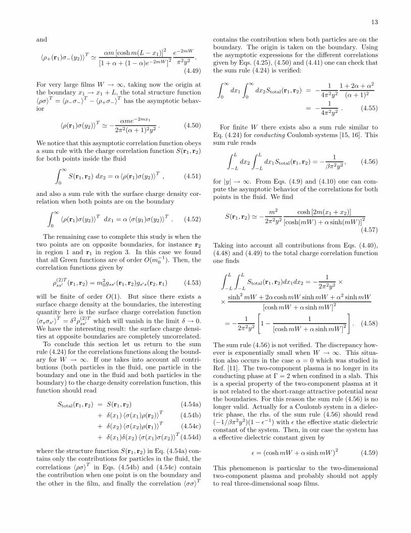
13

and

〈ρ+(r1)σ−(y2)〉T ≃ αm [coshm(L− x1)]2

[1 + α+ (1 − α)e−2mW ]2

e−2mW

π2y2.

(4.49)

For very large films W → ∞, taking now the origin atthe boundary x1 → x1 + L, the total structure function

〈ρσ〉T = 〈ρ−σ−〉T − 〈ρ+σ−〉T has the asymptotic behav-ior

〈ρ(r1)σ(y2)〉T ≃ − αme−2mx1

2π2(α+ 1)2y2. (4.50)

We notice that this asymptotic correlation function obeysa sum rule with the charge correlation function S(r1, r2)for both points inside the fluid

∫ ∞

0

S(r1, r2) dx2 = α 〈ρ(r1)σ(y2)〉T , (4.51)

and also a sum rule with the surface charge density cor-relation when both points are on the boundary

∫ ∞

0

〈ρ(r1)σ(y2)〉T dx1 = α 〈σ(y1)σ(y2)〉T . (4.52)

The remaining case to complete this study is when thetwo points are on opposite boundaries, for instance r2

in region 1 and r1 in region 3. In this case we foundthat all Green functions are of order O(m−1

0 ). Then, thecorrelation functions given by

ρ(2)Tss′ (r1, r2) = m2

0gss′(r1, r2)gs′s(r2, r1) (4.53)

will be finite of order O(1). But since there exists asurface charge density at the boundaries, the interestingquantity here is the surface charge correlation function

〈σsσs′ 〉T = δ2ρ(2)Tss′ which will vanish in the limit δ → 0.

We have the interesting result: the surface charge densi-ties at opposite boundaries are completely uncorrelated.

To conclude this section let us return to the sumrule (4.24) for the correlations functions along the bound-ary for W → ∞. If one takes into account all contri-butions (both particles in the fluid, one particle in theboundary and one in the fluid and both particles in theboundary) to the charge density correlation function, thisfunction should read

Stotal(r1, r2) = S(r1, r2) (4.54a)

+ δ(x1) 〈σ(x1)ρ(r2)〉T (4.54b)

+ δ(x2) 〈σ(x2)ρ(r1)〉T (4.54c)

+ δ(x1)δ(x2) 〈σ(x1)σ(x2)〉T (4.54d)

where the structure function S(r1, r2) in Eq. (4.54a) con-tains only the contributions for particles in the fluid, the

correlations 〈ρσ〉T in Eqs. (4.54b) and (4.54c) containthe contribution when one point is on the boundary and

the other in the film, and finally the correlation 〈σσ〉T

contains the contribution when both particles are on theboundary. The origin is taken on the boundary. Usingthe asymptotic expressions for the different correlationsgiven by Eqs. (4.25), (4.50) and (4.41) one can check thatthe sum rule (4.24) is verified:

∫ ∞

0

dx1

∫ ∞

0

dx2Stotal(r1, r2) = − 1

4π2y2

1 + 2α+ α2

(α + 1)2

= − 1

4π2y2. (4.55)

For finite W there exists also a sum rule similar toEq. (4.24) for conducting Coulomb systems [15, 16]. Thissum rule reads

∫ L

−L

dx2

∫ L

−L

dx1Stotal(r1, r2) = − 1

βπ2y2, (4.56)

for |y| → ∞. From Eqs. (4.9) and (4.10) one can com-pute the asymptotic behavior of the correlations for bothpoints in the fluid. We find

S(r1, r2) ≃ − m2

2π2y2

cosh [2m(x1 + x2)]

[cosh(mW ) + α sinh(mW )]2

(4.57)

Taking into account all contributions from Eqs. (4.40),(4.48) and (4.49) to the total charge correlation functionone finds

∫ L

−L

∫ L

−L

Stotal(r1, r2)dx1dx2 = − 1

2π2y2×

× sinh2mW + 2α coshmW sinhmW + α2 sinhmW

[coshmW + α sinhmW ]2

= − 1

2π2y2

[

1 − 1

[coshmW + α sinhmW ]2

]

. (4.58)

The sum rule (4.56) is not verified. The discrepancy how-ever is exponentially small when W → ∞. This situa-tion also occurs in the case α = 0 which was studied inRef. [11]. The two-component plasma is no longer in itsconducting phase at Γ = 2 when confined in a slab. Thisis a special property of the two-component plasma at itis not related to the short-range attractive potential nearthe boundaries. For this reason the sum rule (4.56) is nolonger valid. Actually for a Coulomb system in a dielec-tric phase, the rhs. of the sum rule (4.56) should read(−1/βπ2y2)(1− ǫ−1) with ǫ the effective static dielectricconstant of the system. Then, in our case the system hasa effective dielectric constant given by

ǫ = (coshmW + α sinhmW )2 (4.59)

This phenomenon is particular to the two-dimensionaltwo-component plasma and probably should not applyto real three-dimensional soap films.

14

V. CONCLUSION

We have studied a toy model for electrolytic soap films.Although this model is very simple and gives only quali-tative information for real soap films it is very interestingsince it is a solvable model. Our study of the disjoiningpressure shows that the charging of the boundaries isresponsible of the stability of the film. For strong adhe-sivity α > 1 the film is stable while for weak adhesivityα < 1 large films are not stable. For 0 < α < 1 largefilms collapse to non-zero width small films. This couldbe the equivalent of a collapse to a Common Black Filmsfor our two-dimensional model. For α = 0 unstable largefilms collapse to a film of zero width which could be theequivalent of a Newton Black Film. We can concludethat the Coulomb interaction plays indeed an importantrole in the stability of large films. This is also the casein the one-dimensional model presented in Ref. [4]. Thenit is natural to expect that for real three dimensionalfilms the Coulomb interaction also plays an importantrole in their stability. Of course in real films there areother important interactions that certainly play a role inthe stability of the film and in particular in the stabilityand structure of black films (both Common Black Filmsand Newton Black Films) that have not been taken intoaccount in our simplified model.

We also studied the density profiles and correlationfunctions for this two-dimensional model. The densityprofile near a boundary shows a classical double layered

structure. A fraction of the anions (soap molecules) arestucked in the boundary creating a first layer of negativesurface charge density. The ions in the fluid create thesecond layer of positive charge and thickness given by thescreening length which screens the first layer.

The correlation functions exhibit the usual behavior.In the x-direction across the film they decay exponen-tially with the characteristic screening length. In they-direction parallel to the boundary they decay alge-braically as 1/y2. The total charge correlation function(taking into account all contributions of particles in thefluid and in the boundary) obeys the usual sum rule forCoulomb fluids near a plane wall when W → ∞. For Wfinite, the two-component plasma at Γ = 2 is no longer aconductor and therefore fails to satisfy a sum rule for cor-relations along the boundaries. We also found an inter-esting new fact: the surface charge densities on oppositeboundaries are completely uncorrelated.

Acknowledgments

G. T. would like to thank B. Jancovici for useful dis-cussions concerning the sum rules of Sec. IV. The au-thors acknowledge partial financial support from COL-CIENCIAS and BID through project # 1204-05-10078.G. T. acknowledge support from ECOS Nord/ICFES ac-tion C00P02 of French and Colombian cooperation.

[1] O. Belorgey and J. J. Benattar, Phys. Rev. Lett. 66, 313(1991).

[2] D. Sentenac and J. J. Benattar, Phys. Rev. Lett. 81, 160(1998).

[3] D. S. Dean and D. Sentenac, Europhys. Lett. 38 645(1997)

[4] D. S. Dean, R. R. Horgan and D. Sentenac,J. Stat. Phys. 90, 899 (1998).

[5] F. Cornu and B. Jancovici, J. Chem. Phys. 90, 2444(1989).

[6] B. Jancovici and G. Tellez, J. Stat. Phys. 82, 609 (1996).[7] P. J. Forrester, J. Stat. Phys. 67, 433 (1992).[8] G. Tellez, J. Stat. Phys. 104, 945 (2001).[9] B. Jancovici, G. Manificat and C. Pisani,

J. Stat. Phys. 76, 307 (1994).[10] B. Jancovici and L. Samaj, J. Stat. Phys. 104, 755

(2001).[11] B. Jancovici and G. Manificat, J. Stat. Phys. 68, 1089

(1992).[12] F. Cornu, Mecanique Statistique Classique de Systemes

Coulombiens Bidimensionels: Resultats Exacts,Ph. D. Thesis, Orsay, France (1989).

[13] B. Jancovici, J. Stat. Phys. 28, 43 (1982)[14] B. Jancovici, J. Stat. Phys. 29, 263 (1982)[15] Ph. A. Martin, Rev. Mod. Phys. 60, 1075 (1988)[16] P. J. Forrester, B. Jancovici and E. R. Smith,

J. Stat. Phys. 31, 129 (1983).