Solution and Liquid Crystalline Properties of Sodium Lauroyl ...

Solution and Liquid

Crystalline Properties of Sodium Lauroyl Methyl

Isethionate/Water Mixtures

A Thesis submitted to The University of Manchester for the degree of Doctor of Philosophy (PhD) in the

Faculty of Engineering and Physical Sciences

2015

JOSEPH CURTIS FLOOD

School of Chemical Engineering and Analytical Science

2

Table of Contents

TABLE OF CONTENTS .................................................................................................................... 2 LIST OF FIGURES ............................................................................................................................ 7 LIST OF TABLES ............................................................................................................................ 10 ABSTRACT ..................................................................................................................................... 11 DECLARATION ............................................................................................................................... 12 COPYRIGHT STATEMENT ............................................................................................................. 12 ACKNOWLEDGEMENTS ............................................................................................................... 13

2 Surfactants ............................................................................................................................... 14

2.1 Structural Classification ...................................................................................................... 14

2.2 Interfacial Phenomena ........................................................................................................ 15

2.3 Micelle Formation ............................................................................................................... 16

2.4 The Hydrophobic Effect ...................................................................................................... 17

2.5 Micelle Shape and the Critical Packing Parameter ............................................................. 17

2.6 Krafft Boundary ................................................................................................................... 19

2.7 Thermodynamics of Self-Assembly .................................................................................... 20

2.8 Dynamics of Micellisation ................................................................................................... 21

3 Liquid Crystals ......................................................................................................................... 24

3.1 Thermotropic, Lyotropic and Chromonic Liquid Crystals .................................................... 24

3.2 Lyotropic Liquid Crystals ..................................................................................................... 25

3.2.1 Lamellar Phase ............................................................................................................ 25

3.2.2 Hexagonal Phases ....................................................................................................... 26

3.2.3 Cubic Phases ............................................................................................................... 27

3.2.4 Nematic Phases ........................................................................................................... 27

3.2.5 Gel Phases .................................................................................................................. 28

3.2.6 Intermediate Phases .................................................................................................... 29

3.3 Lyotropic Liquid Crystal Phase Ordering ............................................................................ 30

4 Common Formulation Additives ............................................................................................ 33

4.1 Electrolytes ......................................................................................................................... 33

4.2 Cosurfactants ...................................................................................................................... 34

4.3 Mixed Micelle Formation ..................................................................................................... 35

3

5 Experimental Techniques ....................................................................................................... 40

5.1 Polarising Optical Microscopy ............................................................................................. 40

5.1.1 Birefringence ................................................................................................................ 40

5.1.2 Phase Identification ..................................................................................................... 41

5.2 Differential Scanning Calorimetry ....................................................................................... 42

5.2.1 Instrumentation and Thermodynamics ........................................................................ 42

5.3 Rheology ............................................................................................................................. 44

5.3.1 Newtonian and Non-Newtonian Fluids ........................................................................ 44

5.3.2 Thixotropy, Rheopexy and Viscoelasticity ................................................................... 47

5.4 X-ray Diffraction .................................................................................................................. 47

5.4.1 Introduction to X-rays ................................................................................................... 48

5.4.2 Bragg’s Law ................................................................................................................. 48

5.4.3 Small Angle X-ray Scattering ....................................................................................... 50

5.4.4 Wide Angle X-ray Scattering ........................................................................................ 51

5.5 Dynamic Light Scattering .................................................................................................... 51

5.5.1 Correlation Function, Z-average Diameter and Polydispersity .................................... 51

5.6 Static Light Scattering ......................................................................................................... 53

5.6.1 Rayleigh Ratio and the Zimm Equation ....................................................................... 53

5.7 Nuclear Magnetic Resonance Spectroscopy ...................................................................... 54

5.7.1 Spin Physics ................................................................................................................ 54

5.7.2 Nuclear Energy Levels in a Magnetic Field ................................................................. 55

5.7.3 Spin-Lattice Relaxation ................................................................................................ 56

5.7.4 Spin-Spin Relaxation ................................................................................................... 57

5.7.5 Nuclear Relaxation Mechanisms ................................................................................. 57

5.7.6 Relaxation Processes in Surfactant Systems .............................................................. 58

6 Sodium Lauroyl Methyl Isethionate Production and Materials ........................................... 60

6.1 Industrial Production of Sodium Lauroyl Methyl Isethionate ............................................... 60

6.2 Materials ............................................................................................................................. 61

7 Aqueous Phase Behaviour of the Sodium Lauroyl Methyl Isethionate/ Water System .... 65

4

7.1 Methodology ....................................................................................................................... 65

7.2 Experimental Method .......................................................................................................... 65

7.2.1 Optical Microscopy ...................................................................................................... 65

7.2.1.1 Phase Penetration Scan ....................................................................................... 65

7.2.1.2 Optical Microscopy of Aqueous Samples ............................................................. 66

7.2.1.3 Experimental Setup .............................................................................................. 66

7.2.2 Small Angle X-Ray Scattering ..................................................................................... 66


7.2.3 Wide Angle X-Ray Scattering ...................................................................................... 67


7.2.4 Differential Scanning Calorimetry ................................................................................ 68


7.3 Results and Discussion ...................................................................................................... 69

7.3.1 Phase Characterisation – Optical Microscopy ............................................................. 69

7.3.2 Phase Characterisation – Small Angle X-ray Scattering (SAXS) ................................ 71

7.3.3 Phase Characterisation – Wide angle X-ray Scattering (WAXS) ................................. 73

7.3.4 Lamellar - Crystal + Isotropic Phase Boundary Determination: Differential Scanning

Calorimetry ............................................................................................................................... 74

7.3.5 Lamellar + Isotropic - Crystal + Isotropic Phase Boundary Determination: Visual

Identification ............................................................................................................................. 76

7.3.1 Sodium Lauroyl Methyl Isethionate/ Water Phase Diagram ........................................ 76

7.4 Conclusions and Future Work ............................................................................................ 78

8 Rheological Performance Properties in Sodium Lauroyl Methyl Isethionate/ {(3-

Dodecanoylamino)propyl(dimethyl)amino}acetate/ Water Mixtures and the Effects of

Process Components .................................................................................................................... 79

8.1 Thickening in Surfactant Mixtures ....................................................................................... 79

8.2 Methodology ....................................................................................................................... 80

8.2.1 Effects on Rheological Performance Caused by Variable Discharge Time ................. 80

8.2.2 Effects of Process Components .................................................................................. 80


5

8.3.1 Effects on Rheological Performance Caused by Variable Discharge Time ................. 80

8.3.2 Effects of Process Components .................................................................................. 81

8.3.3 Experimental Setup ..................................................................................................... 82

8.3.4 Rheological Measurements ......................................................................................... 82


8.4.1 Effects on Rheological Behaviour Induced by Variable Reactor Discharge Time ....... 83

8.4.2 Process Component Effects ........................................................................................ 86

8.5 Conclusions and Future Work ............................................................................................ 89

9 Micelle Build-up Kinetics in the Sodium Lauroyl Methyl Isethionate/

(Carboxylatomethyl)hexadecyldimethyl ammonium /Water System ........................................ 90

9.1 Theoretical Descriptions of Micelle Build-up ....................................................................... 90

9.2 Monitoring Micelle Growth: NMR Linewidth Broadening and Static Light Scattering ......... 91

9.3 Methodology ....................................................................................................................... 93


9.4.1 Phase Diagram Determination ..................................................................................... 93

9.4.2 NMR Spectroscopy ...................................................................................................... 94


9.4.3 Static Light Scattering .................................................................................................. 95



9.5.1 Sodium Lauroyl Methyl Isethionate/ (Carboxylatomethyl) hexadecyldimethyl

ammonium / H2O Partial Phase Diagram ................................................................................. 96

9.5.2 Solution State Proton NMR of Surfactant Components ............................................... 97

9.5.3 Micelle Build-up Kinetics as a Function of Surfactant Concentration ........................ 101

9.5.4 Micelle Build-up Kinetics as a Function of SLMI:Cetyl Betaine Mass Ratio .............. 103

9.6 Conclusions and Future Work .......................................................................................... 105

10 Electrolyte Induced Precipitation in the Sodium Lauroyl Methyl Isethionate/Water

System .......................................................................................................................................... 106

10.1 Clouding in Surfactant Systems ...................................................................................... 106

6

10.2 Introduction to Colloidal Interactions ............................................................................... 107

10.3 Methodology ................................................................................................................... 108

10.4 Experimental Method ...................................................................................................... 108

10.4.1 Cloud Point Determination ....................................................................................... 108

10.4.2 Dynamic Light Scattering ......................................................................................... 109

10.4.2.1 Experimental Setup .......................................................................................... 109

10.4.3 Static Light Scattering .............................................................................................. 109

10.4.3.1 Experimental Setup .......................................................................................... 109

10.5 Results and Discussion .................................................................................................. 110

10.5.1 Anion Effects ............................................................................................................ 110

10.5.2 Cation Effects .......................................................................................................... 112

10.5.3 Salt-Induced Cloud Point Mechanism ...................................................................... 115

10.6 Conclusions and Future Work ........................................................................................ 116

11 Research Summary ............................................................................................................. 117

12 References ........................................................................................................................... 118

Word count: 35,945

7

List of Figures

Figure 2.1. Examples of surfactant types by head group classification. R represents an atom or functional group [2]. ............................................................................................................... 14

Figure 2.2. Surfactant adsorption at the air-water interface. ............................................................ 15 Figure 2.3. Mean dynamic shape of surfactants and the structures they form [10]. ........................ 18 Figure 2.4. Surfactant concentration as a function of temperature for sodium decyl sulphate in

aqueous solution. TKrafft is determined as the intersection between CMC and solubility curves [5, 13]. .................................................................................................................................... 20

Figure 2.5. Dissociation and monomer-micelle exchange constants k-1 as a function of carbon chain length for various alkyl surfactants. CnTAB are alkyltrimethylammonium bromide surfactants, CnK are potassium alkanecarboxylate surfactants, SAS are sodium alkyl sulfate surfactants and CnPyBr are alkylpyridinium bromide surfactants. Circles and squares indicate results from ultrasonic relaxation experiments and those of T- and P-jump studies respectively [19]. .................................................................................................................... 22

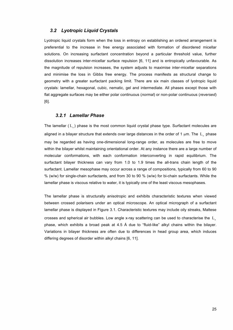
Figure 3.1. Polarisation micrograph showing the Maltese cross patterns of the αL mesophase in an alkylpolyglucoside/water system [25]. .................................................................................... 26

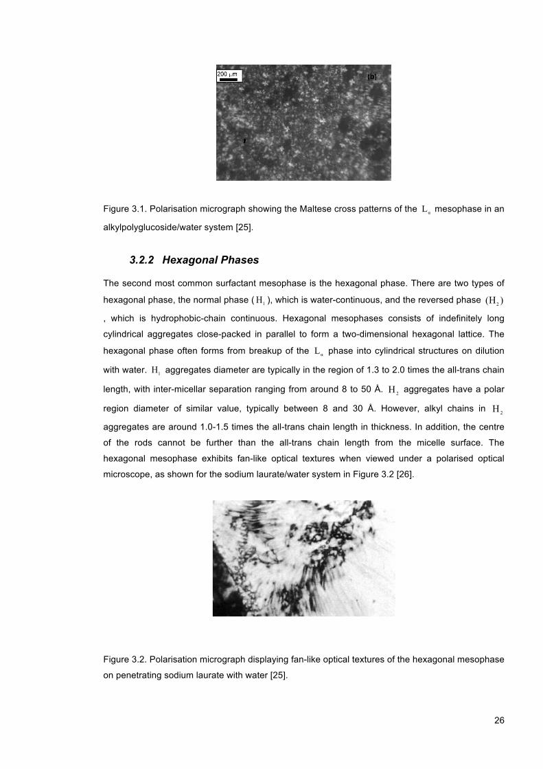
Figure 3.2. Polarisation micrograph displaying fan-like optical textures of the hexagonal mesophase on penetrating sodium laurate with water [25]. ...................................................................... 26

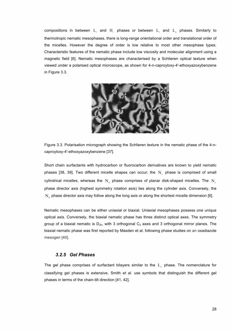
Figure 3.3. Polarisation micrograph showing the Schlieren texture in the nematic phase of the 4-n-caproyloxy-4'-ethoxyazoxybenzene [37]. ............................................................................... 28

Figure 3.4. Graphical representations of the three gel phases according to chain-tilt classification: (a) normal, (b) tilted and (c) inter-digitated. ........................................................................... 29

Figure 3.5. General temperature-water (% w/w) phase sequence of reversed mesophases. ......... 32 Figure 4.1. CMC as a function of surfactant mole fraction 1x , or the micellar mole fraction x1

m , for the SDS + NP-E10 system [58]. .............................................................................................. 36

Figure 4.2. CMC for mixtures of sodium decyl sulphate (SDeS) and decyltrimethylammonium bromide (DeTAB (C10TBR)) as a function of surfactant composition in solution. The dashed line corresponds to an ideal system when 0=β and the solid curve corresponds to the non-ideal case when 2.13−=β [58]. ............................................................................................ 38

Figure 4.3. The micellar composition for mixtures of sodium decyl sulphate (SDeS) and decyltrimethylammonium bromide (DeTAB (C10TBR)). The dashed line corresponds to the ideal case when 0=β and the solid curve corresponds to the non-ideal case when

2.13−=β [58]. ....................................................................................................................... 38

Figure 5.1. Illustration depicting light travelling through non-birefringent isotropic (left) and birefringent anisotropic (right) materials. ............................................................................... 41

Figure 5.2. Illustration of a typical DSC experiment. 1 is the sample material, 2 is the reference material, 3 are temperature sensors, 4 is a thermal conductor and 5 is a heating element. Φo is the temperature of the heating element and ΔT is the temperature difference between sample and reference materials [63]. .................................................................................... 42

Figure 5.3. Two parallel plates with an intervening sheared fluid. The upper plane moves with force F and velocity υ relative to the lower plane [58]. ................................................................ 45

Figure 5.4. Plot of shear stress versus shear rate for various Newtonian and non-Newtonian fluid types [58]. .............................................................................................................................. 45

Figure 5.5. Shear-thinning in dilute and concentrated surfactant systems [58]. D is the shear rate. ............................................................................................................................................... 46

Figure 5.6. Two x-ray beans scattering from Bragg planes. Lattice planes are formed by the atoms, which are depicted by spheres. ............................................................................................. 49

8

Figure 5.7. (a) Nuclear spin energy of a single nucleus of I =1 plotted as a function of magnetic field strength, B0 . (b) Alignment of magnetic vectors in relation to B0 . ................................. 55

Figure 6.1. Surface tension of SLMI/water solutions plotted as a function of SLMI concentration. Measurements were collected at 22.0 °C using the Wilhelmy plate technique and the CMC was determined to be 1.5×10-3 mol kg-1. The reaction scheme for the SLMI production process is as follows: ............................................................................................................. 60

Figure 7.1. Phase penetration experimental setup. Mesophases develop in between the point of solvent contact and the solid surfactant phase [97]. .............................................................. 66

Figure 7.2. Phase penetration scan of SLMI (14055sp composite) by water across the 10.0 to 90.0 °C temperature range. From left to right the phase assignments in each image are crystal; H

aL; 1

Ha L+L 1L . The red magnification line represents 100 µm. ................................................ 69

Figure 7.3. Polarised optical images of SLMI/water (14055sp composite) samples. The red magnification bar represents 100 µm. ................................................................................... 70

Figure 7.4. X-ray d-spacing curves of SLMI/water samples at 22.0 °C: 51.0 (circle), 53.0 (triangle) and 55.0 (plus) % (w/w). ........................................................................................................ 72

Figure 7.5. WAXS scattering curves of a) SLMI (51.0 % (w/w), 25.0 °C) and b) SLMI (51.0 % (w/w), 15.0 °C). ................................................................................................................................. 73

Figure 7.6. WAXS scattering curves of SLMI/water samples using batch 14055sp composite: a) 51.0 % (w/w), 13.0 °C and b) 56.0 % (w/w), 25.0 °C. The appearance of multiple sharp peaks in b) indicates the transition to a crystal phase. .......................................................... 74

Figure 7.7. DSC curves of SLMI/water (14055sp composite) samples at a) 40.0 %, b) 51.0 %, c) 53.0 % and d) 55.0 % (w/w). .................................................................................................. 75

Figure 7.8. Phase diagram for the SLMI/water system. Dotted lines indicate experimentally determined phase boundaries. The dashed line indicates an approximate phase boundary and was determined through visual observation. It is also important to note that phase boundaries at high temperatures are approximately given due to the possibility of sample degradation (hydrolysis). L1 , La

H+L1 , LaH and crystal + L1 regions are indicated. Phase

boundary data points represent an average property using SLMI batch 14055sp: first discharged, composite and last discharged. .......................................................................... 77

Figure 8.1. Plot of viscosity versus shear rate using the base formulation (SLMI batch 14054sp composite) at variable NaCl concentrations (0.0 (triangle), 0.4 (diamond) and 0.6 (cross) % (w/w)). .................................................................................................................................... 83

Figure 8.2. Salt-thickening curves of the base formulation (see Table 8.1) using SLMI batch 14054sp: first discharged (triangle), composite (circle) and last discharged (cross). Lines are drawn as a guide to the eye. .................................................................................................. 84

Figure 8.3. Salt-thickening curves of the base formulation (see Table 8.1) using SLMI batch 14054sp: first discharged (triangle), composite (circle) and last discharged (cross). Lines are drawn as a guide to the eye. .................................................................................................. 84

Figure 8.4. Salt-thickening curves of the base formulation using: (a) batch 14055sp (composite) and (b) batch 14054sp (last discharged). Samples are doped with 0.00 (triangle), 0.11 (circle) and 0.22 % (w/w) PGD (cross). Lines are drawn as a guide to the eye. ................... 86

Figure 8.5. Salt-thickening curves of the base formulation using: (a) batch 14055sp (composite) and (b) batch 14054sp (last discharged) at 0.00 (triangle), 0.23 (circle) and 0.46 (cross) % (w/w) SMI. Lines are drawn as a guide to the eye. ................................................................ 87

Figure 8.6. Salt-thickening curves of the base formulation using: (a) batch 14055sp (composite) and (b) batch 14054sp (last discharged), doped with 0.00 (triangle), 0.29 (circle) and 0.57 (cross) % (w/w) LA. Lines are drawn as a guide to the eye. .................................................. 88

Figure 9.1. Phase diagram depicting the sub-10 % (w/w) total surfactant concentration regime in the SLMI/cetyl betaine/H20 system. ....................................................................................... 96

Figure 9.2. 1H NMR spectrum of sodium lauroyl methyl isethionate (5.0 % (w/w)) in D2O. ............. 98

9

Figure 9.3. 1H NMR spectrum of cetyl betaine (5.0 % (w/w)) in D2O. .............................................. 99 Figure 9.4. 1H NMR spectrum of SLMI/cetyl betaine/D2O (5.0 % (w/w) surfactant. SLMI:cetyl

betaine ratio 1:2 (w:w)). ....................................................................................................... 100 Figure 9.5. (a) Photon count rate and (b) NMR linewidth as a function of time for 2.0 (cross), 3.0

(triangle), 4.0 (circle) and 5.0 (diamond) % (w/w) SLMI/cetyl betaine/water mixtures (SLMI:cetyl betaine ratio 1:2 (w:w)). Equation 9.7 is fitted to both sets of data, as indicated by the black lines. ..................................................................................................................... 101

Figure 9.6. Micelle build-up rate constant k as a function of surfactant concentration at a SLMI:cetyl betaine at a ratio of 1:2 (w:w)). Data was collected using NMR (cross) and SLS (triangle) experiments. Lines are drawn as guides to the eye. ............................................ 102

Figure 9.7. (a) Photon count rate and (b) NMR linewidth of SLMI β-CH2 resonance signal as a function of time for SLMI/cetyl betaine/water mixtures at a fixed total surfactant concentration of 2.0 % (w/w) for SLMI:cetyl betaine ratios of 1:1 (cross), 2:3 (triangle), 1:2 (circle) and 1:3 (plus) (w:w). Equation 9.7 is fitted to the data and is indicated by black lines. .................... 103

Figure 9.8. Micelle build up rate constant k for SLMI/cetyl betaine/water mixtures (2.0 % (w/w)) as a function of SLMI:cetyl betaine mass ratio. NMR (cross) and LS (triangle) data are plotted. ............................................................................................................................................. 104

Figure 10.1. Salt-induced cloud point curves of SLMI/water samples at 20.0 °C. Salts used were Na2HPO4 (cross), NaCl (plus), NaNO3 (triangle) and NaSCN (circle). At SLMI concentrations below ~0.1 mol/kg (indicated by the dotted line), demixing resulted in isotropic phase separation. At SLMI concentrations above ~0.1 mol/kg, demixing resulted in Lα phase

separation from a L1 phase. Solid lines are drawn as a guide to the eye. .......................... 110

Figure 10.2. Plots of (a) hydrodynamic diameter dH , (b) polydispersity index χ and (c) count rate φ of micelles as a function of salt concentration prior to the cloud point in SLMI/water samples (0.1 mol/kg). The salts used were Na2HPO4 (cross), NaCl (plus), NaNO3 (triangle) and NaSCN (circle). All experiments were conducted at 20.0 °C. Lines are drawn as a guide to the eye. ............................................................................................................................ 111

Figure 10.3. Salt-induced precipitation/cloud point curves of SLMI/water samples at 20.0 °C. The salts used were NH4Cl (cross), KCl (plus), LiCl (circle) and NaCl (triangle). At SLMI/water compositions below ~0.1 mol/kg (indicated by the dotted line) demixing resulted in L1 phase separation. At SLMI/water concentrations above ~0.1 mol/kg, demixing resulted in Lα phase

separation from a L1 phase. Solid lines are drawn as a guide to the eye. .......................... 113

Figure 10.4. Plots of (a) hydrodynamic diameter dH , (b) polydispersity index χ and (c) count rate φ of micelles as a function of salt concentration in SLMI/water samples. The salts used were NH4Cl (cross) and LiCl (triangle) and NaCl (circle). All experiments were conducted using SLMI (0.1 mol/kg) at 20.0 °C. Lines are drawn as a guide to the eye. ................................ 114

10

List of Tables

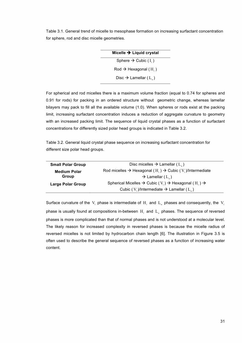
Table 3.1. General trend of micelle to mesophase formation on increasing surfactant concentration for sphere, rod and disc micelle geometries. ......................................................................... 31

Table 3.2. General liquid crystal phase sequence on increasing surfactant concentration for different size polar head groups. ........................................................................................... 31

Table 6.1. Compositional details of SLMI batches (a) 14054sp and (b) 14055sp. .......................... 61 Table 6.2. Compositional details of Natrlquest E30. ........................................................................ 62 Table 6.3. Compositional details of cocamidopropyl betaine. .......................................................... 62 Table 6.4. Compositional details of cetyl betaine. ............................................................................ 62 Table 6.5. Compositional details of freeze-dried cetyl betaine (assuming complete sublimation of

water and ethanol). ................................................................................................................ 62 Table 6.6. Molecular structures of research components. ............................................................... 63 Table 7.1. Summary of optical microscopy data used for construction of the La

H+L1 - 1L phase boundary in SLMI/water samples. The data represents an average property of SLMI batch 14055sp: first discharged, composite and last discharged. ................................................... 71

Table 7.2. Summary of SAXS data and calculations of head group area at 22.0 °C. The standard deviation in d spacing was ± 0.2 Å (using batch 14055sp composite). ................................. 72

Table 7.3. DSC cooling data of SLMI/water LaH phase samples. Enthalpy and transition temperature

represents an average property using SLMI batch 14055sp: first discharged, composite and last discharged. ...................................................................................................................... 75

Table 7.4. Data collected for determining the LaH+L1 -

1L + crystal phase boundary by visual observation, with aid of a temperature controlled water bath. Transition temperature represents an average property using SLMI batch 14055sp: first discharged, composite and last discharged. ...................................................................................................................... 76

Table 8.1. Compositional details of stock solution. .......................................................................... 81 Table 8.2. Compositional details of stock solutions. x was manually doped to yield process

component concentrations at 150 % and 200 % (w/w) of the standard process component concentration in the base formulation. ................................................................................... 81

Table 8.3. Percentage difference Δ(%) of material components between first and last discharged samples in SLMI batches 14054sp and 14055sp. Δ(%) = ( flast − ffirst ) / ffirst where ffirst is the percentage (w/w) of a component is in first discharged material and flast is the percentage (w/w) of a component in last discharged material. ................................................................. 85

Table 9.1. 1H NMR peak assignments of SLMI in D20 (5.0 % (w/w)). H’s (Int.) is the integrated peak intensity and was calculated using Topspin software. H’s is the actual number of protons. . 97

Table 9.2. 1H NMR peak assignments of cetyl betaine in D20 (5.0 % (w/w)). .................................. 97 Table 10.1. Salt-induced surface tension increment and calculated surface tension increments at

the cloud point at 20.0 °C for NaNO3[164], NH4Cl [165], LiCl[34], NaCl[166], NaSCN[167] and Na2HPO4 [168]. ............................................................................................................. 115

11

Abstract

School: The University of Manchester Student name: Joseph Curtis Flood Thesis Title: Solution and Liquid Crystalline Properties of Sodium

Lauroyl Methyl Isethionate/Water Mixtures Submission Date: 23/01/2015 The project contributes to the general theme of complex chemical systems and strengthens ties with Innospec, a multi-national chemical company. Sodium lauroyl methyl isethionate (SLMI. Trade name “Iselux”) is a newly developed surfactant with attractive product properties for personal care applications. Little is known about the fundamental surface and solution properties of SLMI, and it is not currently possible to use information on available surfactants to predict phase behaviour. We characterise the solution and liquid crystalline phase behaviour of the SLMI/water system using a combination of optical microscopy, x-ray scattering and differential scanning calorimetry techniques. SLMI is synthesised using a batch process that leads to variable component concentrations. Preliminary studies conducted by Innospec indicate that the presence of particular process components has a significant influence on SLMI formulation rheological properties. We investigate the effects of synthesis-derived components on the rheological properties of the SLMI/sodium {(3-(dodecanoyl amino)propyl)(dimethyl)ammonio)}acetate/water system using rheology and light scattering (static and dynamic) techniques. SLMI is often formulated into personal care products on mixing aqueous formulation components. Micelle growth occurs via a mechanistic process that is not understood and the equilibrium viscosity is attained at a time after mixing that ranges from seconds to weeks. Developing an improved understanding of the micelle growth mechanism is of both academic and industrial value. We utilise static light scattering and nuclear magnetic resonance techniques to probe a range of samples in the viscoelastic region of the SLMI/(carboxymethyl)hexadecyl dimethylammonium hydroxide/water system. Experimental findings improve our current understanding of micelle growth process and provide a platform for future research on non-equilibrium mixing kinetics. In the final section we investigate salt-induced cloud point and precipitation phenomena in the SLMI/salt/water system. The cloud point is commonly observed in surfactant and protein systems by increasing the solution temperature above a critical value, resulting in phase separation of solute-rich and solute-depleted layers. Cloud point induced phase separation may also be prompted by addition of salt. The mechanistic process driving electrolyte-induced cloud point phenomena is not understood. We use a combination of turbidimetry measurements and light scattering (static and dynamic) techniques to measure cloud point curves and characterise micellar behaviour prior to clouding.

12

Declaration

I declare that that no portion of the work referred to in the thesis has been submitted in support of

an application for another degree or qualification of this or any other university or other institute of

learning.

Copyright Statement

i. The author of this thesis (including any appendices and/or schedules to this thesis) owns

certain copyright or related rights in it (the “Copyright”) and s/he has given The University

of Manchester certain rights to use such Copyright, including for administrative purposes.

ii. Copies of this thesis, either in full or in extracts and whether in hard or electronic copy, may

be made only in accordance with the Copyright, Designs and Patents Act 1988 (as

amended) and regulations issued under it or, where appropriate, in accordance with

licensing agreements which the University has from time to time. This page must form part

of any such copies made.

iii. The ownership of certain Copyright, patents, designs, trademarks and other intellectual

property (the “Intellectual Property”) and any reproductions of copyright works in the thesis,

for example graphs and tables (“Reproductions”), which may be described in this thesis,

may not be owned by the author and may be owned by third parties. Such Intellectual

Property and Reproductions cannot and must not be made available for use without the

prior written permission of the owner(s) of the relevant Intellectual Property and/or

Reproductions.

iv. Further information on the conditions under which disclosure, publication and

commercialisation of this thesis, the Copyright and any Intellectual Property and/or

Reproductions described in it may take place is available in the University IP Policy (see

http://documents.manchester.ac.uk/DocuInfo.aspx?DocID=487), in any relevant Thesis

restriction declarations deposited in the University Library, The University Library’s

regulations (see http://www.manchester.ac.uk/library/aboutus/regulations) and in The

University’s policy on Presentation of Theses.

13

Acknowledgements

First I am thankful to my supervisor and friend, Dr Robin Curtis, who gave me the opportunity to

work on this PhD project. Robin has provided excellent mentorship and eased my transition from

physical science into chemical engineering. He is a wonderful supervisor and I am yet to meet

anyone who can explain thermodynamics with such clarity after so much beer.

My foremost thankfulness is reserved for Professor Gordon Tiddy. You inspire me to reach higher

and I am truly privileged to have worked under your supervision. I am infinitely grateful for your

humour, time, enthusiasm, guidance, expertise and wisdom. Our “early morning” meetings were a

highlight of my week and something I always looked forward to.

I would also thank my industrial sponsor, Innospec, for funding part of the project. My gratitude is

extended to Dr Ian McRobbie, Dr Nick Dixon and Dr Tony Gough, for their guidance and support. I

also would like to thank the EPSRC for their funding contributions.

My acknowledgments are extended to my Masters students who inspired key ideas and were

integral to delivering a successful project. Thank you to Flora, Asima, Daniel, Aim and Karishma.

I’d also like to acknowledge the people who have made my journey a lot smoother. Thank you for

the unforgettable memories Abdullatif, Helen, Max, Spyros, James, Rose, David, Marium, Ishara,

Vicky, Rafael and Jennifer.

Ultimately I would like to thank my remarkable parents, Nigel and Peggy Flood. Thank you for your

unconditional love, guidance, motivation and support.

14

2 Surfactants

2.1 Structural Classification

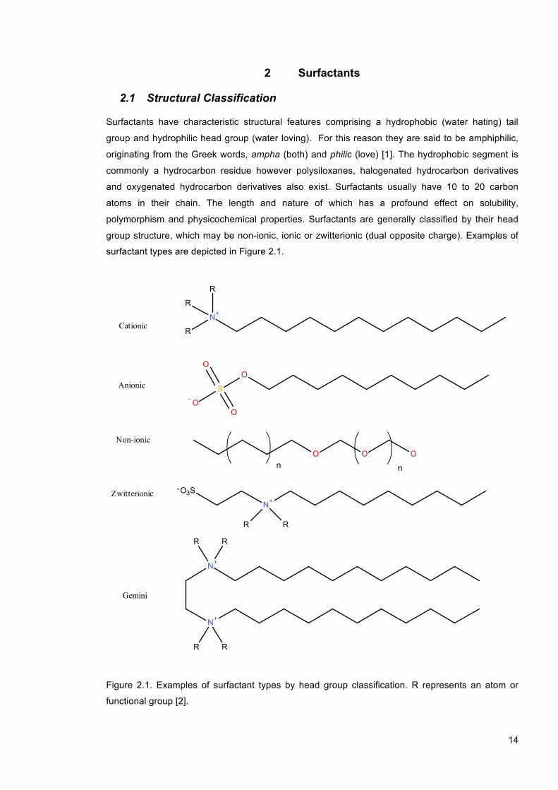
Surfactants have characteristic structural features comprising a hydrophobic (water hating) tail

group and hydrophilic head group (water loving). For this reason they are said to be amphiphilic,

originating from the Greek words, ampha (both) and philic (love) [1]. The hydrophobic segment is

commonly a hydrocarbon residue however polysiloxanes, halogenated hydrocarbon derivatives

and oxygenated hydrocarbon derivatives also exist. Surfactants usually have 10 to 20 carbon

atoms in their chain. The length and nature of which has a profound effect on solubility,

polymorphism and physicochemical properties. Surfactants are generally classified by their head

group structure, which may be non-ionic, ionic or zwitterionic (dual opposite charge). Examples of

surfactant types are depicted in Figure 2.1.

n n

Cationic

Anionic

Non-ionic

Zwitterionic

Gemini

Figure 2.1. Examples of surfactant types by head group classification. R represents an atom or

functional group [2].

-

15

2.2 Interfacial Phenomena

When a surfactant is dissolved in a polar solvent, the system will minimise free energy by expelling

hydrophobic tail-solvent contacts via the hydrophobic effect (see Section 2.4), which is achieved by

adsorption of surfactant to the interface and/or formation of sub-microscopic colloidal particles

called micelles.

Surfactants preferentially adsorb at the air-water interface as shown in Figure 2.2. When adsorbed

at the interface, the surfactants hydrophilic segment is immersed in water and the hydrophobic

segment partitions at the air-water interface. The alignment and aggregation of surfactant

molecules at the water/air interface acts to reduce the free energy of interaction between air and

water, which in turn reduces interfacial tension [3].

Figure 2.2. Surfactant adsorption at the air-water interface.

The change in surface tension of a pure surfactant in solution is governed by the Gibbs adsorption

isotherm [4]

Γ(1) = −1RT

dγd(lnc)#

$%

&

'(T ,P

Equation 2.1

where Γ(1) is the Gibbs surface excess of the surfactant, γ is the interfacial tension and c is the

total surfactant concentration. The isotherm assumes ideal solution behaviour and zero solvent

concentration at the surface. For concentrated solutions the surfactant activity ( a =ψc , where ψ is

the activity coefficient of the surfactant) should be used instead of concentration. The isotherm

16

requires that an increase in concentration of a component with positive surface excess induce a

reduction in surface tension.

For dissociative species such as ionic surfactants, the isotherm becomes

Γ(1) = −12RT

dγd(lnc)#

$%

&

'(T ,P

Equation 2.2

In the case of swamping electrolyte or when ionic strength is high enough to negate electrostatic

effects, Equation 2.1 applies.

2.3 Micelle Formation

Surfactant functionality originates from molecular structure, with the polar head-group conveying

water solubility and the non-polar tail driving surface adsorption or self-assembly. If the polar and

apolar segments of a molecule are not sufficiently well defined, the system can phase separate and

monomer aggregation may not occur without the aid of additives. Examples of such molecules

include most ketones, aldehydes and simple ethers [5].

Micelles result from surfactant self-assembly at concentrations above the critical micelle

concentration (CMC). The CMC is not a single value, since micelle formation occurs over a narrow

concentration range [6]. However, the concentration range is usually extremely small so that for

most purposes, it is convenient to specify a single value.

In single surfactant systems at concentrations below the CMC, all surfactant exists in monomeric

form. At concentrations greater than or equal to the CMC, some of the dissolved surfactant self-

assembles to form micelles. For surfactant mixtures the solution behaviour is more complex, as

there will be multiple CMC values for each respective surfactant.

Structural features of a surfactant, such as hydrophobic chain length and type of head group affect

the CMC. Increasing the number of carbon atoms in the hydrophobic tail group lowers the CMC

value due to an increased contribution of the hydrophobic effect [1]. As the hydrophobic chain

length increases, the Gibbs free energy of transferring the hydrocarbon chain into a micelle within a

polar solvent becomes increasingly negative [5]. Head group size and classification also affects the

CMC. Bulky and highly charged a surfactant head groups induce a significant loss in entropy on

micellisation, which leads to an increased CMC. Such entropic losses originate from repulsive

hydration forces, steric hindrance and electrostatic effects.

17

2.4 The Hydrophobic Effect

The hydrophobic effect drives surfactant adsorption and self-assembly and is a term used to

describe the unfavourable interaction between an apolar solute and water. The first and most

significant contribution to the hydrophobic effect arises from a loss in entropy due to the reduction

in hydrogen bonding configurations available to the water molecules surrounding the solute. The

second contribution to the hydrophobic effect originates in the energy required to overcome the

strong cohesive forces between water molecules and create a cavity for the apolar molecule. The

magnitude of the hydrophobic effect is directly proportional to the hydrophobic solute-water contact

area [6].

Repulsion between polar head groups opposes self-assembly. The origin of this lateral repulsion is

complex and a number of factors require consideration. When polar head groups move closer

together they dehydrate and experience a repulsive hydration force. Thermal fluctuations also

decrease because of steric hindrance, further reducing mobility. For ionic surfactants, there is an

additional electrostatic contribution associated with the energy required to push charged head

groups closer together. The magnitude of electrostatic head-group repulsion means ionic

surfactants generally have a higher CMC than non-ionic counterparts [6, 7].

2.5 Micelle Shape and the Critical Packing Parameter

Micelles exist in a variety of geometries; small globules, oblate or prolate ellipsoids, long cylinders,

flat disks and reversed structures have all been observed. Micelles can form bilayer structures

which may be rigid or flexible, the latter making it possible to form vesicle structures [8]. Geometric

transformations can occur when solution conditions such as the ionic strength, pH and/or

temperature are changed.

Globular micelles are characterised by a small aggregation number, Ns ≈ 10 to 150, and positive

surface curvature. Surfactant monomers that form globular micelles often possess a short

hydrocarbon chain attached to a bulky head group [9]. In contrast, rod micelles exhibit much larger

aggregation numbers and can grow to several hundred nanometres in size. Surfactant molecules

that form rod micelles generally possess long hydrocarbon tail segments and a less bulky head

group relative to surfactants that form spherical micelles [9]. The geometry of a micelle is related to

surfactant molecular structure via the critical packing parameter, which is described in the following

paragraph.

The critical packing parameter (CPP =ν a0lc ) relates optimal head-group area a0 , hydrophobic

chain volume ν and critical chain length lc . The CPP is a dimensionless number that reflects the

shape a molecule can adopt in an aggregate. Several different structures can satisfy a single CPP

value, however entropy will favour the structure with the smallest aggregation number [10].

18

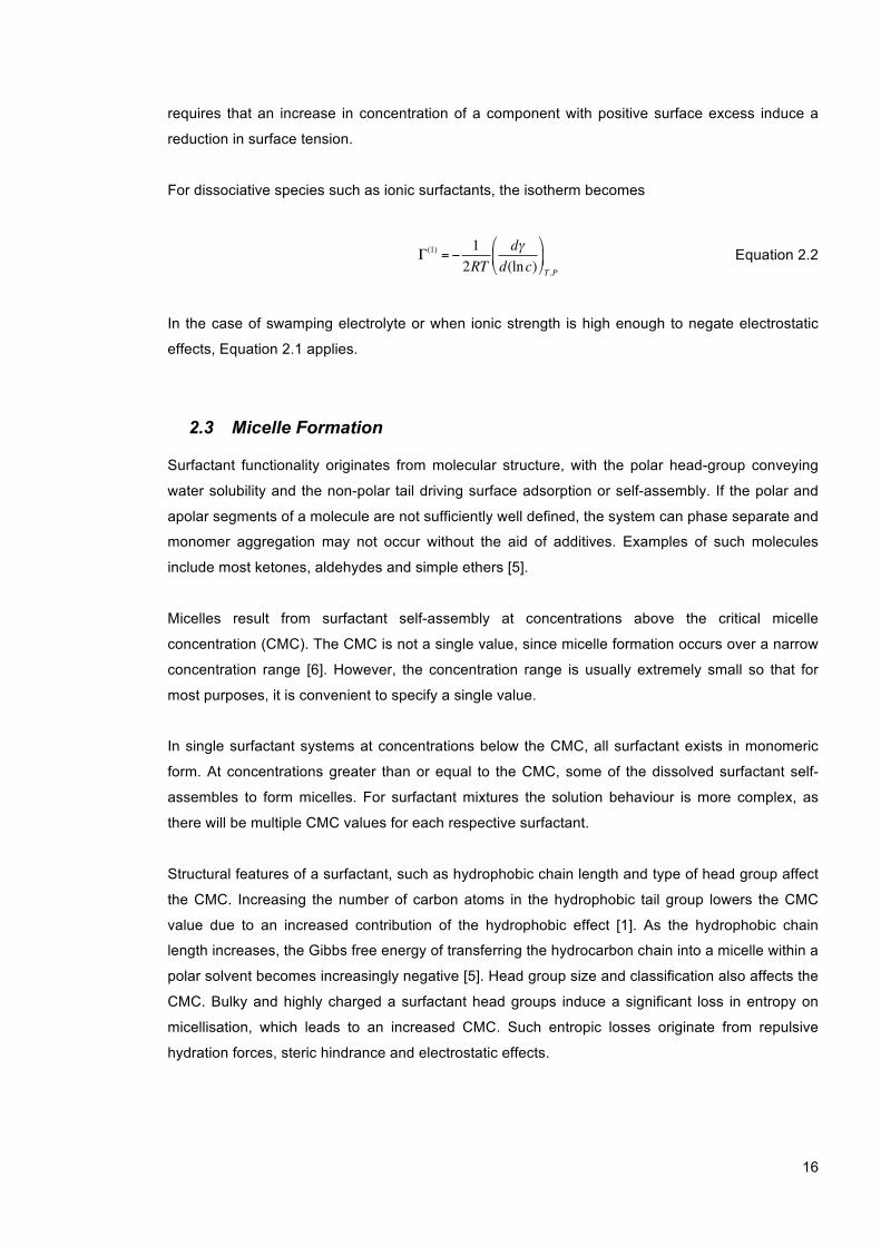
As the CPP increases, there is a change of preferred structure from spherical micelles

(0 ≤ν a0lc ≤1/ 3) to rod-like micelles (1 / 3≤ν a0lc ≤1/ 2) to various interconnected structures

(1 / 2 ≤ν a0lc ≤1) to vesicles, bilayers and reversed structures (ν a0lc ≥1) . The various micelle

shapes are summarised in Figure 2.3 [10].

Figure 2.3. Mean dynamic shape of surfactants and the structures they form [10].

Varying solution conditions may induce a micelle structural transition by affecting the following

factors:

19

1. a0 . Surfactants with small head-group areas may form structures with less positive surface

curvatures such as large vesicles, bilayers or inverted micellar phases. Shape changes can be

induced by addition of electrolyte or additional components that alter the value of a0 . Ionic

surfactant systems generally increase in a0 (and decrease in micelle size) as a function of

temperature due to increases in thermal motion [11]. Non-ionic polyoxyethylene surfactants

often exhibit a decrease in a0 (and increase in micelle size) function of temperature. Several

theories have been proposed in attempt to explain the phenomenon and a widely accepted

theoretical description is yet to be presented. One of the most common theories [12] suggests

that increases in micelle size as a function of temperature are attributed to reduction in inter-

head group repulsion. The decrease in inter-head group repulsion is thought to occur as a

result of weakening favourable head group-solvent interactions due to temperature-induced

broadening in the distribution of preferred head group conformations. For zwitterionic

surfactants, temperature generally has less of an effect on micelle size.

2. Chain packing ( lc and ν ). Hydrocarbon chain branching and other structural factors such as

unsaturated cis-double bonding reduce lc and increase the CPP . The same effect may be

achieved by adding small amounts of organic molecules that can penetrate into the micelle and

increase ν . The aforementioned effects can promote formation of larger aggregates and yield

inverted structures.

3. Mixed systems. When the system contains a mixture of amphiphilic components, aggregate

properties may be treated in terms of a mean packing parameter, provided that there is ideal

mixing and no phase separation. Micelle sizes may be increased or decreased, depending on

the type of additive used. In practice, mixed micelle systems generally exhibit non-ideal

behaviour due to physical effects (steric, spatial) and interactions between head groups,

hydrocarbon tails and external molecules.

2.6 Krafft Boundary

To form micelles the system temperature must exceed a particular value known as the Krafft

temperature (TKrafft). TKrafft occurs at the intersection of the solubility curve and CMC curve [5] and is

indicated in Figure 2.4, which shows a plot of surfactant concentration as a function of temperature

in the sodium decyl sulphate/water system. If the system temperature is below TKrafft, only

surfactant monomers exist in equilibrium with the hydrated crystalline surfactant. Above TKrafft

micelles form to induce a rapid increase in surfactant solubility.

20

Figure 2.4. Surfactant concentration as a function of temperature for sodium decyl sulphate in

aqueous solution. TKrafft is determined as the intersection between CMC and solubility curves [5,

13].

TKrafft is dependent on structural characteristics of a surfactant that affect solubility and packing

efficiency in crystal form, such as chain length and branching. From an industrial viewpoint, it is

often important to operate above the Krafft boundary to ensure product functionality. Chain

branching, double bonds and/or polar segments between the alkyl chain and head group act to

reduce crystal packing efficiency and lower TKrafft [5].

2.7 Thermodynamics of Self-Assembly

Tanford (1980) published a simplified yet extremely useful description of micelle aggregation, which

was later extended to larger aggregates such as bilayers, vesicles and microemulsion droplets [10].

Tanford’s thermodynamic description of micellar aggregation is known as the Multiple Equilibrium

Model and treats micellisation as a series of step-wise, co-operative equilibrium steps [14]. The

model implies coexistence of different micelle sizes, where the distribution of surfactant between a

range of aggregation states is described by a series of dynamic equilibria [1]:

Si−1 + S1⇔ Si Equation 2.3

with equilibrium constant Ki

21

Ki = Si Si−1S1 Equation 2.4

where S1 is the concentration of surfactant monomers and Si is the concentration of aggregates of

i monomers. At equilibrium the chemical potential of each identical molecule in different

aggregates is the same.

µ = µ10 +KbT logX1 = µ2

0 +12KbT logX2 = µi

0 +1iKbT logXi = ... Equation 2.5

It follows that

µi = µi0 +

KbTilogXi Equation 2.6

where µi is the mean chemical potential of a monomer in an aggregate of i monomers, µi0 is the

standard chemical potential of a monomer in aggregates of i monomers, Xi is the activity per

monomer in aggregates of i monomers ( iii SaX = ) and ia is the activity coefficient of the

surfactant monomer. An expression for the total surfactant concentration, C is given by

C = XNN=1

∞

∑ Equation 2.7

A necessary condition for the formation of stable aggregates is that µN0 < µ1

0 for some value(s) of

N (µN0 has a minimum value at some finite value of N ).

2.8 Dynamics of Micellisation

Surfactant monomers are in dynamic equilibrium with micelles and the aggregation number

represents a time-averaged value. The kinetics of micellisation scales with the CMC. Lower CMC

values promotes slower aggregation/break-up dynamics by influencing [6]:

1. The monomer-micelle exchange rate. The rate of entry of monomers into the micelles is

diffusion controlled. Ultrasonic studies have indicated this process occurs on the microsecond

timescale [15, 16].

2. The micelle lifetime (dissociation). Surfactants with a high CMC are able to reach the micelle

surface quickly relative to surfactants with a low CMC. However, increases in CMC correlate

with reduction in surface activity. T (temperature)-jump and P (pressure)-jump studies have

22

indicated that the dissociation of a micelle into monomers occurs on the millisecond timescale

[17, 18].

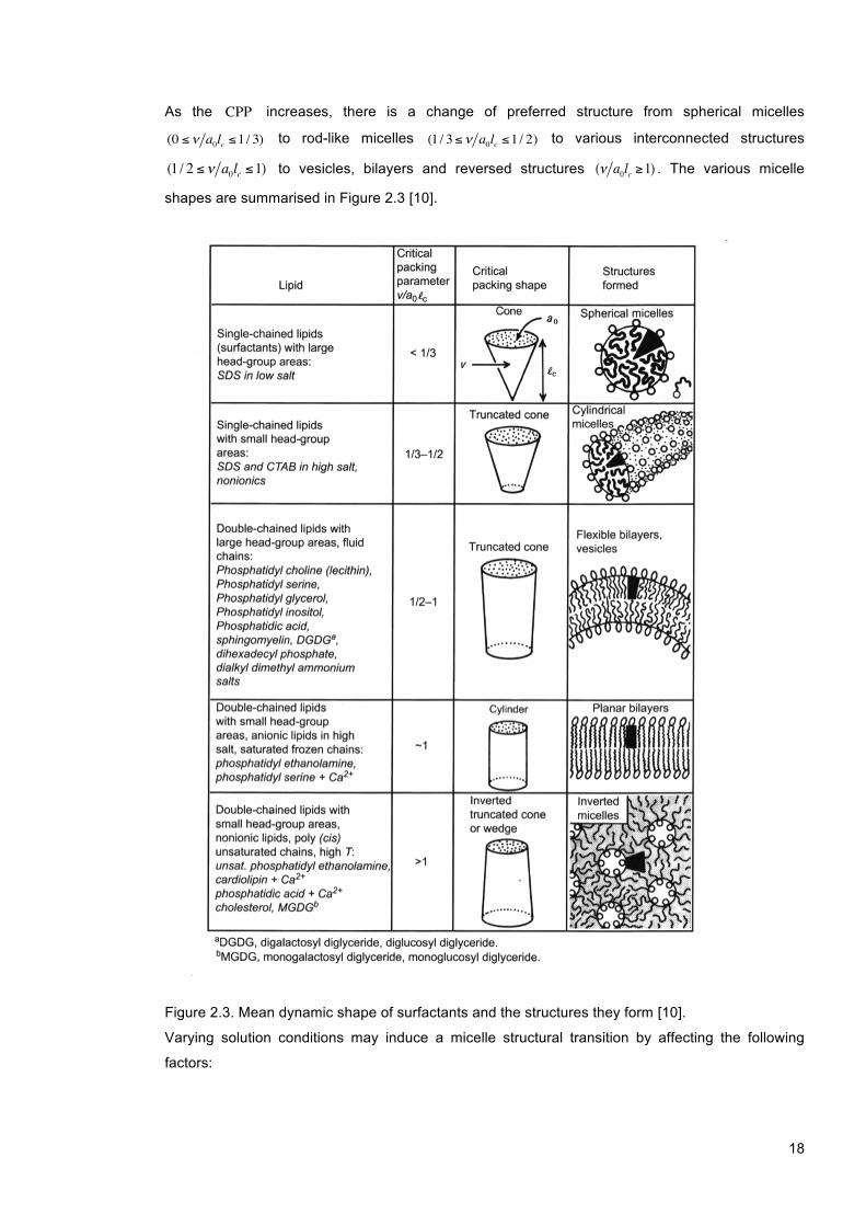
Hydrophobic bonding forces are stronger for molecules with longer alkyl chains and consequently

the monomer-micelle exchange rate is dependent on chain length. In Figure 2.5 is a plot of

monomer micelle exchange and dissociation rate constants (k-1) as a function of the number of

carbon atoms for a series of alkyl surfactants.

Figure 2.5. Dissociation and monomer-micelle exchange constants k-1 as a function of carbon

chain length for various alkyl surfactants. CnTAB are alkyltrimethylammonium bromide surfactants,

CnK are potassium alkanecarboxylate surfactants, SAS are sodium alkyl sulfate surfactants and

CnPyBr are alkylpyridinium bromide surfactants. Circles and squares indicate results from

ultrasonic relaxation experiments and those of T- and P-jump studies respectively [19].

The experimentally determined curves for monomer-micelle exchange rates show little dependence

on the head group type, but instead depend on hydrophobic chain length [1, 19]. Micelle kinetics

can be probed non-invasively by measuring the local motions within alkyl chains using multi-field

NMR experiments. The molecular motion at various points along the alkyl chain can be quantified

using “fast” (local motion of alkyl chain segments) and “slow” (tumbling of the whole aggregate

and/or diffusion of surfactant monomers over the surface) correlation times [20]. In normal micelles,

23

the “fast” motion becomes more rapid as distance from the polar head group increases. At the end

of the alkyl chain furthest from the polar head group, correlation times of the “fast” motion occur in

the order of 10-11 seconds, which is similar to that of pure liquid hydrocarbons of similar length and

is indicative of a liquid-like micelle interior.

Monovalent counterions exhibit rapid exchange rates at the micelle surface (10-8 to 10-9 s),

indicating high lateral mobility and implying that there are no associations to a specific head group

[21]. Bound water molecules have also been studied using NMR and self-diffusion. Experimental

data indicates that bound water molecules exhibit fast exchange rates (10-8 s), however water

rotation rates are slower than that of bulk water molecules [1].

24

3 Liquid Crystals

3.1 Thermotropic, Lyotropic and Chromonic Liquid Crystals

Solid crystals possess well-defined three dimensional phase structures, with ordered molecular

arrangements (molecules are volumetrically confined) and regular periodicity extending over many

structural planes. Conversely, molecules in a liquid exhibit random molecular motion and assume

the shape of a container. Rheologically, liquids and solids exhibit different behaviours. Liquids flow

under applied stress whereas solids exhibit considerably higher resistance to deformation.

Liquid crystals exhibit intermediate properties of liquid and solid phases. There is some degree of

long-range positional order and molecular tumbling, which may be anisotropic. Many types of liquid

crystal phases (mesophases) occur with varying levels of molecular mobility and structural order.

Some mesophases interchange with other phases via first-order phase transitions, representing a

change in molecular entropy at a particular temperature. Liquid crystal phase transitions generally

exhibit small transition enthalpies relative to solid-liquid transitions [6, 11].

Liquid crystals are commonly divided into two subcategories known as “thermotropic” or “lyotropic”.

Mesophases formed by changing temperature are thermotropic, whereas those formed by solvent

dissolution are lyotropic. Dividing liquid crystals into either thermotropic or lyotropic materials does

not allow for simple distinction as many mesophases exhibit properties of both.

Thermotropic liquid crystals often comprise of molecules possessing a flexible hydrocarbon chain

connected to a rigid polyaromatic head group. Molecular order arises from the anisotropic

molecular shape and short-range anisotropic attraction between molecules. Thermotropic

“character” originates from changes in molecular conformation induced by temperature change. An

example of a compound exhibiting thermotropic liquid crystal behaviour is para-azoxyanisole [22].

The thermotropic nematic phase can be aligned by an external magnetic or electric field, leading to

applications in liquid crystal display (LCD) technology [23].

Lyotropic liquid crystals comprise semi-ordered arrays of solvated amphiphilic molecular

aggregates known as micelles. Micelles are significantly larger than solvent molecules and their

translational order arises from inter-aggregate repulsion at increased solute concentrations.

Lyotropic liquid crystals commonly occur in solutions of phospholipids, fatty acid salts, polymers

and biological macromolecules. Chromonics are a sub-category of lyotropic liquid crystal that often

derive from polyaromatic compounds with polar substituents. Chromonics form multi-molecular

aggregates via π-stacking interactions, as opposed to the hydrophobic effect that is found in

lyotropic systems [24]. The following section is an overview of lyotropic liquid crystals found in

surfactant systems. Thermotropic and chromonic liquid crystals were not researched and a

comprehensive review is beyond the scope of study.

25

3.2 Lyotropic Liquid Crystals

Lyotropic liquid crystals form when the loss in entropy on establishing an ordered arrangement is

preferential to the increase in free energy associated with formation of disordered micellar

solutions. On increasing surfactant concentration beyond a particular threshold value, further

dissolution increases inter-micellar surface repulsion [6, 11] and is entropically unfavourable. As

the magnitude of repulsion increases, the system adjusts to maximise inter-micellar separations

and minimise the loss in Gibbs free energy. The process manifests as structural change to

geometry with a greater surfactant packing limit. There are six main classes of lyotropic liquid

crystals: lamellar, hexagonal, cubic, nematic, gel and intermediate. All phases except those with

flat aggregate surfaces may be either polar continuous (normal) or non-polar continuous (reversed)

[6].

3.2.1 Lamellar Phase

The lamellar ( αL ) phase is the most common liquid crystal phase type. Surfactant molecules are

aligned in a bilayer structure that extends over large distances in the order of 1 µm. The αL phase

may be regarded as having one-dimensional long-range order, as molecules are free to move

within the bilayer whilst maintaining orientational order. At any instance there are a large number of

molecular conformations, with each conformation interconverting in rapid equilibrium. The

surfactant bilayer thickness can vary from 1.0 to 1.9 times the all-trans chain length of the

surfactant. Lamellar mesophase may occur across a range of compositions, typically from 60 to 90

% (w/w) for single-chain surfactants, and from 30 to 90 % (w/w) for bi-chain surfactants. While the

lamellar phase is viscous relative to water, it is typically one of the least viscous mesophases.

The lamellar phase is structurally anisotropic and exhibits characteristic textures when viewed

between crossed polarisers under an optical microscope. An optical micrograph of a surfactant

lamellar phase is displayed in Figure 3.1. Characteristic textures may include oily streaks, Maltese

crosses and spherical air bubbles. Low angle x-ray scattering can be used to characterise the αL

phase, which exhibits a broad peak at 4.5 Å due to “fluid-like” alkyl chains within the bilayer.

Variations in bilayer thickness are often due to differences in head group area, which induces

differing degrees of disorder within alkyl chains [6, 11].

26

Figure 3.1. Polarisation micrograph showing the Maltese cross patterns of the αL mesophase in an

alkylpolyglucoside/water system [25].

3.2.2 Hexagonal Phases

The second most common surfactant mesophase is the hexagonal phase. There are two types of

hexagonal phase, the normal phase ( 1H ), which is water-continuous, and the reversed phase )(H2

, which is hydrophobic-chain continuous. Hexagonal mesophases consists of indefinitely long

cylindrical aggregates close-packed in parallel to form a two-dimensional hexagonal lattice. The

hexagonal phase often forms from breakup of the αL phase into cylindrical structures on dilution

with water. 1H aggregates diameter are typically in the region of 1.3 to 2.0 times the all-trans chain

length, with inter-micellar separation ranging from around 8 to 50 Å. 2H aggregates have a polar

region diameter of similar value, typically between 8 and 30 Å. However, alkyl chains in 2H

aggregates are around 1.0-1.5 times the all-trans chain length in thickness. In addition, the centre

of the rods cannot be further than the all-trans chain length from the micelle surface. The

hexagonal mesophase exhibits fan-like optical textures when viewed under a polarised optical

microscope, as shown for the sodium laurate/water system in Figure 3.2 [26].

Figure 3.2. Polarisation micrograph displaying fan-like optical textures of the hexagonal mesophase

on penetrating sodium laurate with water [25].

27

Hexagonal phases are viscous in comparison to the αL phase, but not relative to cubic and gel

phases. Small angle x-ray diffraction studies on hexagonal phases yield Bragg reflections in the

ratio 1:1 / √3:1 / √4:1 / √7:1, etc., with a diffuse reflection at 4.5 Å .

3.2.3 Cubic Phases

Cubic mesophases are viscous isotropic structures based around one of several possible cubic

lattices: primitive (P), face-centred (F) and body-centred (I) [5, 6]. Cubic mesophases comprise of

two sub-types. The first cubic sub-type comprises a three-dimensional discontinuous array of small

micelles (normal or reversed), which is labelled “ I ”. The second sub-type is based on three

dimensional bicontinuous aggregates, labelled “V ” (normal or reversed). For the water-continuous

1I phase, several cubic structures have been reported, such as primitive (Pm3n), face-centred

(Fm3m) and body-centred (Im3m). For cubic lattices assigned to the Fm3m and Im3m space

groups, a single quasi-spherical micellar shape has been proposed [27, 28]. Aggregate diameters

are similar to those in normal micellar solutions, with inter-micellar separations comparable with the

1H phase. The structure of cubic Pm3m phases is contested, and some authors suggest that two

different micelle structures coexist, with one micelle being slightly larger than the other [27-30].

Whether the micelles are short rods or flattened spheres are currently unknown. Fairly recently, a

model suggested by Seddon et al. states that the structure may be composed of two spherical

micelles and six disc-shaped micelles [28].

For the reverse cubic 2I phase, an Fd3m structure containing 24 micelles of two distinct sizes has

been found. The coexistence of two different micelle sizes is more probable with reversed

structures as the alkyl chain packing constraints no longer limit the micelle diameter. Bicontinuous

cubic phases (V ) commonly possess one of three main space groups, Pn3n, Im3m and Ia3d [31-

34]. Aggregates form an infinitely extended three-dimensional structure, where most surface

coordinates are saddle points. Once again, the surface may be normal or reversed, depending on

whether the net curvature is positive towards water or oil. The net curvature of the V phase is

intermediate of 1H and αL phases, which is consistent with the composition region in which it is

usually found. The Ia3d structure is currently described as an infinite periodic array of minimal

surfaces [35]. For the 1V phase, only the Ia3d space group has been reported, whereas 2V

mesophases are found to exhibit the three space groups (Pn3m, Im3m and Ia3d). I and V cubic

classes are distinguished by their position on phase diagrams. I occurs between 1L and 1H

phases, while V phases occur between 1H and αL phases.

3.2.4 Nematic Phases

Nematic phases in lyotropic systems were first reported by Lawson and Flautt [36] and are fairly

uncommon relative to the mesophases previously discussed. Nematic phases may exist at

28

compositions in between 1L and 1H phases or between 1L and αL phases. Similarly to

thermotropic nematic mesophases, there is long-range orientational order and translational order of

the micelles. However the degree of order is low relative to most other mesophase types.

Characteristic features of the nematic phase include low viscosity and molecular alignment using a

magnetic field [6]. Nematic mesophases are characterised by a Schlieren optical texture when

viewed under a polarised optical microscope, as shown for 4-n-caproyloxy-4'-ethoxyazoxybenzene

in Figure 3.3.

Figure 3.3. Polarisation micrograph showing the Schlieren texture in the nematic phase of the 4-n-

caproyloxy-4'-ethoxyazoxybenzene [37].

Short chain surfactants with hydrocarbon or fluorocarbon derivatives are known to yield nematic

phases [38, 39]. Two different micelle shapes can occur; the cN phase is comprised of small

cylindrical micelles, whereas the dN phase comprises of planar disk-shaped micelles. The cN

phase director axis (highest symmetry rotation axis) lies along the cylinder axis. Conversely, the

dN phase director axis may follow along the long axis or along the shortest micelle dimension [6].

Nematic mesophases can be either uniaxial or biaxial. Uniaxial mesophases possess one unique

optical axis. Conversely, the biaxial nematic phase has three distinct optical axes. The symmetry

group of a biaxial nematic is D2h, with 3 orthogonal C2 axes and 3 orthogonal mirror planes. The

biaxial nematic phase was first reported by Masden et al. following phase studies on an oxadiazole

mesogen [40].

3.2.5 Gel Phases

The gel phase comprises of surfactant bilayers similar to the αL phase. The nomenclature for

classifying gel phases is extensive. Smith et al. use symbols that distinguish the different gel

phases in terms of the chain-tilt direction [41, 42].

29

The gel phase is highly viscous and bilayers contain rigid, all-trans hydrocarbon chain structures.

Gel mesophases are characterised by a sharp wide-angle scattering (WAXS) spacing of ~4.2 Å

and a melting enthalpy of ~25 to 75 % of the surfactant crystal melting enthalpy. The melting

enthalpy of the gel phase suggests that there is restricted chain motion, where only rotation about

the long axis can occur.

There are three widely recognised types of gel phase, corresponding to normal, tilted and inter-

digitated, as depicted in Figure 3.4. The normal structure (a) has bilayers normal to the liquid

crystal axis, and is most commonly found in dialkyl lipid systems [43]. Normal gel phases possess

bilayer thicknesses of approximately twice the all-trans surfactant chain length. The tilted structure

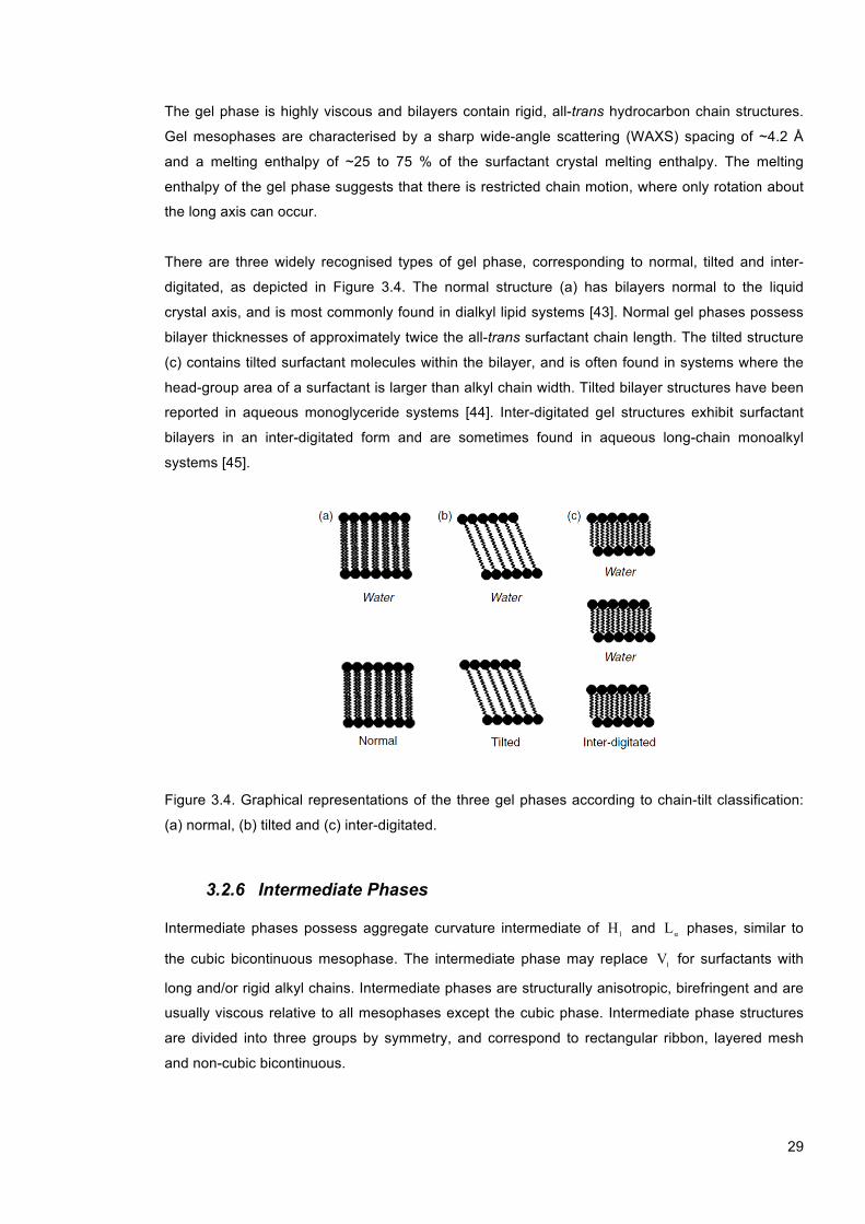
(c) contains tilted surfactant molecules within the bilayer, and is often found in systems where the

head-group area of a surfactant is larger than alkyl chain width. Tilted bilayer structures have been

reported in aqueous monoglyceride systems [44]. Inter-digitated gel structures exhibit surfactant

bilayers in an inter-digitated form and are sometimes found in aqueous long-chain monoalkyl

systems [45].

Figure 3.4. Graphical representations of the three gel phases according to chain-tilt classification:

(a) normal, (b) tilted and (c) inter-digitated.

3.2.6 Intermediate Phases

Intermediate phases possess aggregate curvature intermediate of 1H and αL phases, similar to

the cubic bicontinuous mesophase. The intermediate phase may replace 1V for surfactants with

long and/or rigid alkyl chains. Intermediate phases are structurally anisotropic, birefringent and are

usually viscous relative to all mesophases except the cubic phase. Intermediate phase structures

are divided into three groups by symmetry, and correspond to rectangular ribbon, layered mesh

and non-cubic bicontinuous.

30

The ribbon phases can be considered as a distorted hexagonal phase and are the most extensively

studied of the intermediate phases. Ribbon phases occur when the surfactant molecules aggregate

into long flat ribbons (aspect ratio ca. 0.5), located on two-dimensional lattices of hexagonal,

oblique or rectangular [46]

Mesh intermediate phases are distorted lamellar-like structures in which the continuous bilayers

are split by water-filled defects. The non-cubic bicontinuous intermediate structures are distorted

cubic structures. Mesh intermediate phases are formed by a range of long-chain non-ionic

surfactant systems. There are several possible mesh structures with both tetrahedral and

rhombohedral symmetry [47, 48]. Intermediate phases with reversed curvatures are uncommon,

with only a handful of reports citing their existence. Detailed structural characterisations of the

reversed intermediate phases are not established, nor are the effect of small changes in alkyl chain

length. In reversed structures there is a significant amount of conformational freedom due to the

water present in the core. It is therefore likely for reversed intermediate phases to be found in

systems containing low water volume fractions and multi-chain amphiphiles with bulky head

groups.

3.3 Lyotropic Liquid Crystal Phase Ordering

1I , 1H and αL phases are mesomorphic structures based on ordered arrangements of globular

(spherical), rod and disc micelles respectively. Conversely, intermediate and 1V phases comprise

of aggregates with surface curvature intermediate of rods and discs. The liquid crystal phases

formed and their respective sequences may be predicted by the micelle geometry at the CMC and

the ‘effective’ micelle volume fraction, which dictates micelle packing limits at increased surfactant

concentrations [49]. The ‘effective’ volume fraction comprises the actual volume occupied by chain

groups, head groups and bound water. Also included are the effects of soft-core intermicellar

interactions [5, 10], such as overlapping head group conformations, electrostatics, hydration forces,

ion specificity (adsorption/desorption), polarisable organics and polymers. The combinations of

effects are complex, and it is therefore fortuitous that general mesomorphic behaviour is often

comparable to that of a ‘hard-wall’ particle [6]. The chemical structure of a surfactant has a

profound effect on the concentration ranges over which mesophases are observed, but not the

phase sequence. Micelle shape is determined by the critical packing parameter, which was

discussed in Section 2.5. There is a critical volume fraction above which disordered solutions

cannot occur for spherical and disc micelles. The general scheme for normal (non-reversed)

micelles on increasing surfactant concentration is indicated in Table 3.1.

31

Table 3.1. General trend of micelle to mesophase formation on increasing surfactant concentration

for sphere, rod and disc micelle geometries.

Micelle à Liquid crystal

Sphere à Cubic ( 1I )

Rod à Hexagonal ( 1H )

Disc à Lamellar ( αL )

For spherical and rod micelles there is a maximum volume fraction (equal to 0.74 for spheres and

0.91 for rods) for packing in an ordered structure without geometric change, whereas lamellar

bilayers may pack to fill all the available volume (1.0). When spheres or rods exist at the packing

limit, increasing surfactant concentration induces a reduction of aggregate curvature to geometry

with an increased packing limit. The sequence of liquid crystal phases as a function of surfactant

concentrations for differently sized polar head groups is indicated in Table 3.2.

Table 3.2. General liquid crystal phase sequence on increasing surfactant concentration for

different size polar head groups.

Small Polar Group Disc micelles à Lamellar ( αL )

Medium Polar Group

Rod micelles à Hexagonal ( 1H ) à Cubic ( 1V )/Intermediate à Lamellar ( αL )

Large Polar Group

Spherical Micelles à Cubic ( 1V ) à Hexagonal ( 1H ) à Cubic ( 1V )/Intermediate à Lamellar ( αL )

Surface curvature of the 1V phase is intermediate of 1H and αL phases and consequently, the 1V

phase is usually found at compositions in-between 1H and αL phases. The sequence of reversed

phases is more complicated than that of normal phases and is not understood at a molecular level.

The likely reason for increased complexity in reversed phases is because the micelle radius of

reversed micelles is not limited by hydrocarbon chain length [6]. The illustration in Figure 3.5 is

often used to describe the general sequence of reversed phases as a function of increasing water

content.

32

Figure 3.5. General temperature-water (% w/w) phase sequence of reversed mesophases.

There are a number of surfactants for which the illustration in Figure 3.5 is misrepresentative, as

more than two mesophases have been observed at a given concentration. Furthermore, on

increasing water content some systems exhibit 2/HLα or 22/HV sequences. For all its limitations,

the diagram in Figure 3.5 does indicate which phases are most likely to occur adjacently and is

best used as a rough guide for predicting mesophase sequence.

33

4 Common Formulation Additives

4.1 Electrolytes

Specific ion effects are ubiquitous in surfactant systems. Electrolytes impose a strong influence on

the interaction between micelles and affect aggregation properties of amphiphilic molecules. On

dissolution of ionic surfactants in electrolyte solution, electrostatic interactions induce a significant

reduction of the CMC. The effect on CMC of an electrolyte is more pronounced for anionic and

cationic surfactants than for non-ionic and zwitterionic surfactants [3]. For anionic and cationic

surfactants, the relation between electrolyte concentration and CMC follows the general relation:

bCa i +−= )log()CMClog( Equation 4.1

where a and b are ionic head group constants at a defined temperature and iC is the total

counterion concentration in equivalents per litre. The lowering in the CMC with increasing

electrolyte concentration is attributed to the electrostatic screening effect of electrolyte, which

decreases the size of the ionic atmosphere surrounding the surfactant head groups and reduces

inter-head group electrostatic repulsion. For non-ionic and zwitterionic surfactants, the relation

between electrolyte concentration and surfactant CMC is commonly described by [50]:

sKC−= )CMCln()CMCln( 0 Equation 4.2

where CMC0 is the critical micelle concentration of a surfactant in absence of salt sC is the

concentration of electrolyte (mol/L) and K is an electrolyte and surfactant specific constant at a

defined temperature. The influence of electrolyte on CMC is attributed primarily to salting-in or

salting-out effects of the hydrophobic groups by the electrolyte, as opposed to the head group

effects observed in anionic and cationic systems.

In ionic surfactant solutions the addition of salt above a critical limit results in demixing and phase

separation, also known as clouding or salting-out. Clouding phenomena is a consequence of

attractive interactions between surfactant micelles, and initially yields a cloudy mixture. With time,

the system separates into two coexisting phases. One phase is surfactant-rich and the other

surfactant-depleted. The salting-out ability of an ion is described by the Hofmeister series [51],

which was originally used to describe salting-out of egg-white proteins. The effectiveness of an ion

to induce salting-out follows the order [51]:

Citrate3- ≈ SO42- > PO4

3- > F- > Cl- > Br- > I- > NO3- > ClO4

-

N(CH3)4+ > NH4

+ > Cs+ > Rb+ > K+ > Na+ > H+ > Ca2+ > Mg2+ > Al3+

34

Initial theories to explain ordering of the series were based on the size of hydrated ions and water

structure. Such theories state that small hydrated ions (kosmotropes) increase water structure and

dehydrate the surfactant, defining such ions as effective at salting-out. Conversely, large

dehydrated ions (chaotropes) are said to break-up water-water interactions and increase the level

of surfactant hydration, which increases salting-in potency [1, 51]. The above reasoning is

successful for anions but not cations, primarily because salting-out interactions are balanced by

adsorption interactions, which are strongest for heavily hydrated cations. Thus the salting out

tendency of cations is strongly depends on the interaction with surfactant head groups. The

aforementioned adsorption effects are non-electrostatic and the mechanisms by which they are

manifested are not currently understood [52].

By discussing Hofmeister effects as a series of ions, one neglects that ions are not isolated species

in solution, and they may interact with each other and with surfaces. Ion specificity depends on

counterion type and surface composition. A theory proposed by Collin relates the tendency of

oppositely charged ions to spontaneously associate as inner-sphere ion pairs in aqueous solution

to matching absolute free energies of ion hydration. The success of the concept is attributed to the

fact that the strength of interaction between ions and water molecules correlates with the strength

of ion-ion interactions [53]. An extended computation study by Jungwirth et al. reported ion pairing

of sodium and potassium ions with a broad range of biologically relevant ions in aqueous solution

[54, 55]. A Hofmeister-like head group series was proposed from the results on the study by Kunz

et al. [56].

Hard Soft

Carboxylate > phosphate > sulphate > sulfonate

Kunz et al. demonstrated that using the proposed head group series in combination with the

concept of matching water affinities provided qualitative explanations for a multitude of

experimental data published in recent years [56].

4.2 Cosurfactants

Molecules that are insufficiently hydrophilic to form micelles or mesophases with water alone, but

have profound effects when mixed with surfactants are known as cosurfactants. Examples of

cosurfactant molecules can include alcohols, long chain aldehydes and fatty acids. The magnitude

of polar group hydration affects the level of incorporation of cosurfactant into the mesophase and

the affinity of a polar group for the micelle surface also has an effect on mesophase behaviour.

Weakly polar groups can occupy both the micelle interior and reside at the micelle surface.

35

Ekwall et al. investigated the effects of various cosurfactant additives on the phase behaviour of the

sodium octanoate/water system [57]. Three additives with approximately the same chain length as

sodium octanoate were studied: decanol, octyl aldehyde (octanal) and methyl octanoate. In water,

sodium octanoate formed only a hexagonal phase at room temperature, however increasing

temperature yielded 1V and αL phases. Decanol (head group area ~12 Å2) occupied a large αL

region and a 2H region due to the alcohol functional group residing at the water/alkyl chain

interface. The sodium octanoate head group area is ~58 Å2 in mesophases and packing constraint

calculations predict the occurrence of a α/LH1 transition at a sodium octanoate/decanol weight

ratio of 7:3, which is in agreement with experimental data. Octyl aldehyde and methyl octanoate

are comparatively soluble in the 1H phase, which is likely because they occupy a significant

proportion of the micelle interior. Octanal resides primarily at the micelle surface and induces a αL

phase region, which is in equilibrium with the 1L phase. Methyl isethionate resides primarily in the

micelle interior, and therefore the αL phase does not bound with the 1L phase.

4.3 Mixed Micelle Formation

Surfactant formulations often contain additional surfactant components to increase performance by

tuning solution properties such as the rheology, foaming ability and CMC. Surfactant mixtures form

micelles that may contain a mixture of the amphiphilic components. A theoretical understanding of

mixed micelle formation enables one to derive information on micelle composition and prediction of

CMC values.

For the simplest case of a mixed bi-surfactant system, there is no net interaction between the

surfactant species. The approximation may only be valid if the surfactants possess identical head

groups but different chain lengths. For such systems, it is reasonable to assume that the CMC is a

weighted average of the individual species [58]

∑=ixmi iCMCCMC Equation 4.3

where xim is the mole fraction of surfactant i in the mixed micelle. Equation 4.3 has limited use in

its current form, as xim is not known a priori. If xi is the solution composition, the CMC of a mixed

surfactant system is

∑=i

xiiCMCCMC

1 Equation 4.4

For the simplest case of a bi-surfactant mixture, combining equations 4.3 and 4.4 results in an

expression for the composition of the mixed micelle as a function of iCMC and xi .

36

1221

211 CMCCMC

CMCxx

xxm+

= Equation 4.5

The sodium dodecyl sulphate (SDS)/nonylphenol with 10 ethylene oxide units (NP-E10)/water

system is considered in Figure 4.1, in which the CMC is plotted as a function of the molar

composition of the solution (circles) and the molar composition in the micelles (squares). If the

molar composition of micelles is plotted along the x-axis, the CMC is the arithmetic mean of the

CMC’s of each surfactant (Equation 4.3). Conversely, if the molar composition of the solution is

plotted along the x-axis (CMC is equal to the total molar composition), the CMC drops significantly

at low levels of NP-E10. The trend is explained by preferential absorption of NP-E10 into the micelle,

due to NP-E10 exhibiting a greater hydrophobicity relative to SDS.

Figure 4.1. CMC as a function of surfactant mole fraction 1x , or the micellar mole fraction x1m , for

the SDS + NP-E10 system [58].

For surfactants with different head group structures and/or charges, there is often net interaction

and non-ideal behaviour. Ternary systems that combine anionic and cationic surfactants exhibit

strong net attractions between surfactant head groups due to opposite charged head-groups. To

account for non-ideal interactions between surfactant head-groups, activity coefficient models are

utilised and Equation 4.3 becomes

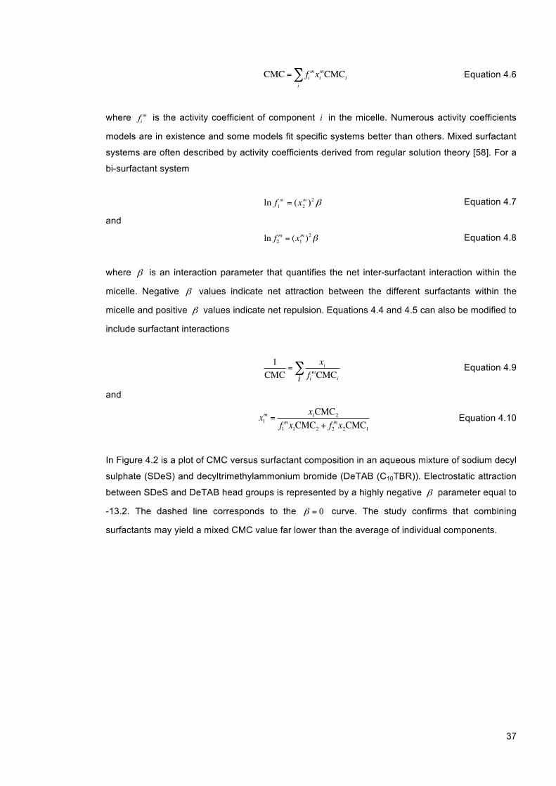
37

CMC = fimxi

mCMCii∑ Equation 4.6

where fim is the activity coefficient of component i in the micelle. Numerous activity coefficients

models are in existence and some models fit specific systems better than others. Mixed surfactant

systems are often described by activity coefficients derived from regular solution theory [58]. For a

bi-surfactant system

β221 )(ln mm xf = Equation 4.7

and

ln f2m = (x1

m )2β Equation 4.8

where β is an interaction parameter that quantifies the net inter-surfactant interaction within the

micelle. Negative β values indicate net attraction between the different surfactants within the

micelle and positive β values indicate net repulsion. Equations 4.4 and 4.5 can also be modified to

include surfactant interactions

1CMC

=xi

fimCMCii

∑ Equation 4.9

and

x1m =

x1CMC2f1mx1CMC2 + f2

mx2CMC1 Equation 4.10

In Figure 4.2 is a plot of CMC versus surfactant composition in an aqueous mixture of sodium decyl

sulphate (SDeS) and decyltrimethylammonium bromide (DeTAB (C10TBR)). Electrostatic attraction

between SDeS and DeTAB head groups is represented by a highly negative β parameter equal to

-13.2. The dashed line corresponds to the 0=β curve. The study confirms that combining

surfactants may yield a mixed CMC value far lower than the average of individual components.

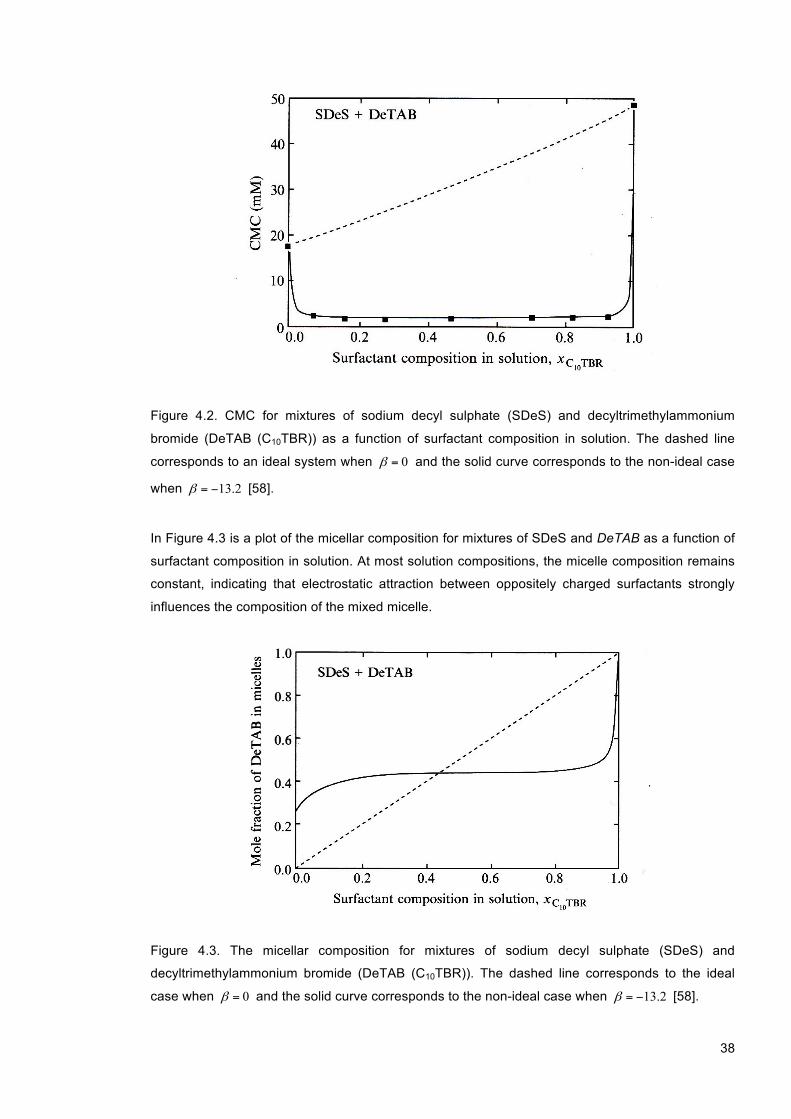
38

Figure 4.2. CMC for mixtures of sodium decyl sulphate (SDeS) and decyltrimethylammonium

bromide (DeTAB (C10TBR)) as a function of surfactant composition in solution. The dashed line

corresponds to an ideal system when 0=β and the solid curve corresponds to the non-ideal case

when 2.13−=β [58].

In Figure 4.3 is a plot of the micellar composition for mixtures of SDeS and DeTAB as a function of

surfactant composition in solution. At most solution compositions, the micelle composition remains

constant, indicating that electrostatic attraction between oppositely charged surfactants strongly

influences the composition of the mixed micelle.

Figure 4.3. The micellar composition for mixtures of sodium decyl sulphate (SDeS) and

decyltrimethylammonium bromide (DeTAB (C10TBR)). The dashed line corresponds to the ideal

case when 0=β and the solid curve corresponds to the non-ideal case when 2.13−=β [58].

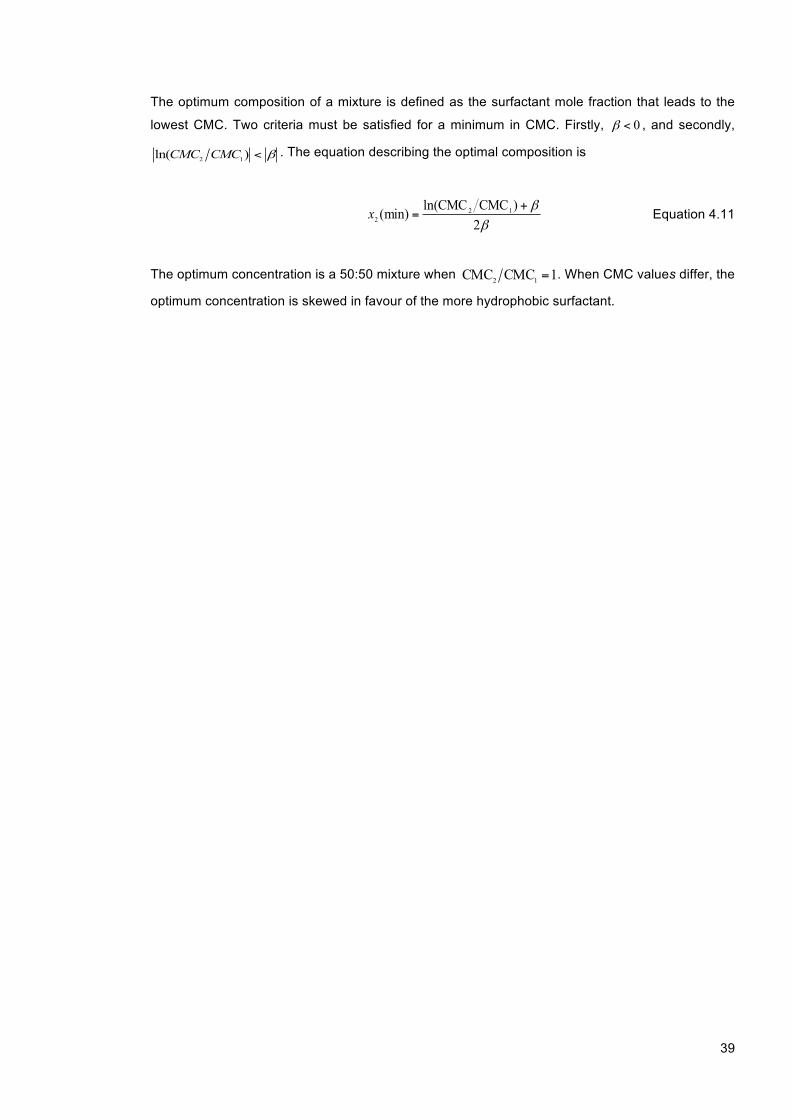
39

The optimum composition of a mixture is defined as the surfactant mole fraction that leads to the

lowest CMC. Two criteria must be satisfied for a minimum in CMC. Firstly, 0<β , and secondly,

β<)ln( 12 CMCCMC . The equation describing the optimal composition is

ββ

2)CMCCMCln((min) 12

2

+=x Equation 4.11

The optimum concentration is a 50:50 mixture when 1CMCCMC 12 = . When CMC values differ, the

optimum concentration is skewed in favour of the more hydrophobic surfactant.

40

5 Experimental Techniques

Various experimental techniques were used to characterise solution and liquid crystalline phase

behaviour of SLMI in aqueous systems. Micellar and liquid crystalline phase behaviour was probed

using x-ray diffraction (wide and small angle), dynamic light scattering, rheology and polarising

optical microscopy. Nuclear magnetic resonance (NMR) spectroscopy was used to follow micellar

build-up processes in SLMI water mixtures. In the following chapter are descriptions of the

techniques utilised to aid research.

5.1 Polarising Optical Microscopy

Polarising optical microscopy is a versatile technique that is used to aid the identification of liquid

crystalline phases. The technique is quick, convenient and generates a significant amount of

information that may be used for preliminary phase identification. Liquid crystals may scatter and

rotate the plane of polarised light, generating characteristic optical textures specific to a particular

phase(s). Structurally anisotropic liquid crystalline phases often possess an optical property known

as optical birefringence, which occurs due to the difference in refractive index as a function of

sample orientation [59, 60].

5.1.1 Birefringence

A polarising optical microscope includes a light source and two polarising light filters placed at right

angles: the polariser and analyser. Polarising light filters only permit light of a specific vibrational

component and adsorb all light with other vibrational components. If the polariser and analyser are

placed at right angles, the polarisers are crossed, and no light can pass due to destructive

interference [61]. Many liquid crystal phases display optical patterns with bright coloured areas

when viewed under a polarising optical microscope. The phenomenon is due to an optical property

known as birefringence, which occurs when the refractive index of the sample material is

dependent on the direction of light propagation. The birefringence of a material is often expressed

as ∆𝑛 = 𝑛!! − 𝑛!, where 𝑛!! and 𝑛! are the refractive indices parallel and perpendicular to the liquid

crystal director axis respectively. The refractive index defines the reduction in speed of light as it

transverses a material. In Figure 5.1 is shown a diagram that depicts light waves passing through

isotropic and anisotropic samples. Light entering the anisotropic sample splits into ordinary (o-) and

extraordinary (e-) rays that travel at different velocities. The change in refractive index results in

brightly coloured textures and the viewing intensity is dependent on sample thickness; thin samples

exhibit brighter textures.

41

Figure 5.1. Illustration depicting light travelling through non-birefringent isotropic (left) and

birefringent anisotropic (right) materials.

In the isotropic sample light is not observed as there is no change in refractive index on passing

through the sample (refractive index is independent of sample orientation) [62]. When polarised

light passes through an isotropic phase, the plane of polarisation (emergence, e-ray) is unchanged

with respect to the incident ray. All the light it absorbed by the analyser and dark regions appear as

the sample is non-birefringent.

5.1.2 Phase Identification

Liquid crystalline phases can exhibit characteristic optical textures when viewed under a polarising

optical microscope. Mesophases may undergo homeotropic alignment, in which the molecules are

aligned via their director axis parallel to the glass sample slide and perpendicular to the viewing

direction. Mesophases exhibiting homeotropic alignment appear optically extinct (the mesophase

appears opaque and black) for planar alignments when the optical axis is parallel to either polariser

axis (θ° = 0, 90, 180, 360). The mesogenic textures are a consequence of phase specific structural

defects.

Lamellar phases often exhibit oily streaks, spherical air bubbles and Maltase cross textures,

whereas hexagonal phases are identifiable from non-spherical air bubbles and fan-like textures.

42

Cubic phases are isotropic and non-birefringent, however may exhibit shear birefringence on

compression. To identify a phase type with confidence, optical microscopy needs to be used in

conjunction with additional techniques such as x-ray diffraction.

5.2 Differential Scanning Calorimetry

Differential scanning calorimetry (DSC) is frequently used in combination with optical microscopy,

x-ray scattering and NMR spectroscopy for phase identification in surfactant systems. DSC is

utilised to probe thermally induced phase transitions and extract thermodynamic data on

crystallisation, glass transition and melting. Qualitative and quantitative information on phase

transitions may be extracted from DSC experiments.

5.2.1 Instrumentation and Thermodynamics

The calorimeter consists of two separate compartments: a sample cell and a reference cell. The

cells are made of platinum for thermal stability at high temperatures. Both cells are connected to

separate temperature sensors and a resistance heater for thermal control. The resistance heater

operates using electrical current and can deliver temperature changes at a specified rate. A typical

DSC setup is drawn in Figure 5.2.

Figure 5.2. Illustration of a typical DSC experiment. 1 is the sample material, 2 is the reference

material, 3 are temperature sensors, 4 is a thermal conductor and 5 is a heating element. Φo is the

temperature of the heating element and ΔT is the temperature difference between sample and

reference materials [63].

The resistance heaters maintain sample and reference materials at constant temperature by

controlling heat flow. Difference in heat flow between sample and reference materials forms the

basis of a DSC experiment. When experiments are conducted at constant pressure, heat flow is

equivalent to enthalpy [64]

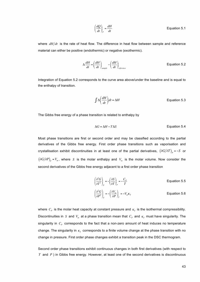
43

dQdt

!

"#

$

%&P

=dHdt

Equation 5.1

where dH dt is the rate of heat flow. The difference in heat flow between sample and reference

material can either be positive (endothermic) or negative (exothermic).

ΔdHdt

=dHdt

"

#$

%

&'sample

−dHdt

"

#$

%

&'reference

Equation 5.2

Integration of Equation 5.2 corresponds to the curve area above/under the baseline and is equal to

the enthalpy of transition.

ΔdHdt

"

#$

%

&'dt∫ = ΔH Equation 5.3

The Gibbs free energy of a phase transition is related to enthalpy by

ΔG = ΔH −TΔS Equation 5.4

Most phase transitions are first or second order and may be classified according to the partial

derivatives of the Gibbs free energy. First order phase transitions such as vaporisation and

crystallisation exhibit discontinuities in at least one of the partial derivatives, ∂G ∂T( )P = −S or

∂G ∂P( )T =Vm , where S is the molar enthalpy and Vm is the molar volume. Now consider the

second derivatives of the Gibbs free energy adjacent to a first order phase transition

∂2G∂T 2

"

#$

%

&'P

= −∂S∂T"

#$

%

&'P

= −CP

T Equation 5.5

∂2G∂P2"

#$

%

&'T

= −∂Vm∂P

"

#$

%

&'T

= −VmκT Equation 5.6

where CP is the molar heat capacity at constant pressure and κT is the isothermal compressibility.

Discontinuities in S and Vm at a phase transition mean that CP and κT must have singularity. The

singularity in CP corresponds to the fact that a non-zero amount of heat induces no temperature

change. The singularity in κT corresponds to a finite volume change at the phase transition with no

change in pressure. First order phase changes exhibit a transition peak in the DSC thermogram.

Second order phase transitions exhibit continuous changes in both first derivatives (with respect to

T and P ) in Gibbs free energy. However, at least one of the second derivatives is discontinuous

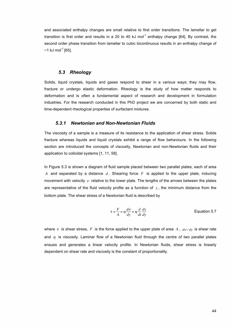
44

and associated enthalpy changes are small relative to first order transitions. The lamellar to gel

transition is first order and results in a 20 to 40 kJ mol-1 enthalpy change [64]. By contrast, the

second order phase transition from lamellar to cubic bicontinuous results in an enthalpy change of

~1 kJ mol-1 [65].

5.3 Rheology

Solids, liquid crystals, liquids and gases respond to shear in a various ways; they may flow,

fracture or undergo elastic deformation. Rheology is the study of how matter responds to

deformation and is often a fundamental aspect of research and development in formulation

industries. For the research conducted in this PhD project we are concerned by both static and

time-dependent rheological properties of surfactant mixtures.

5.3.1 Newtonian and Non-Newtonian Fluids

The viscosity of a sample is a measure of its resistance to the application of shear stress. Solids

fracture whereas liquids and liquid crystals exhibit a range of flow behaviours. In the following

section are introduced the concepts of viscosity, Newtonian and non-Newtonian fluids and their

application to colloidal systems [1, 11, 58].

In Figure 5.3 is shown a diagram of fluid sample placed between two parallel plates, each of area

A and separated by a distance d . Shearing force F is applied to the upper plate, inducing

movement with velocity υ relative to the lower plate. The lengths of the arrows between the plates

are representative of the fluid velocity profile as a function of y , the minimum distance from the

bottom plate. The shear stress of a Newtonian fluid is described by

τ =FA=η

dυdy

=ηddtdxdy

Equation 5.7

where τ is shear stress, F is the force applied to the upper plate of area A , dυ / dy is shear rate

and η is viscosity. Laminar flow of a Newtonian fluid through the centre of two parallel plates

ensues and generates a linear velocity profile. In Newtonian fluids, shear stress is linearly

dependent on shear rate and viscosity is the constant of proportionality.

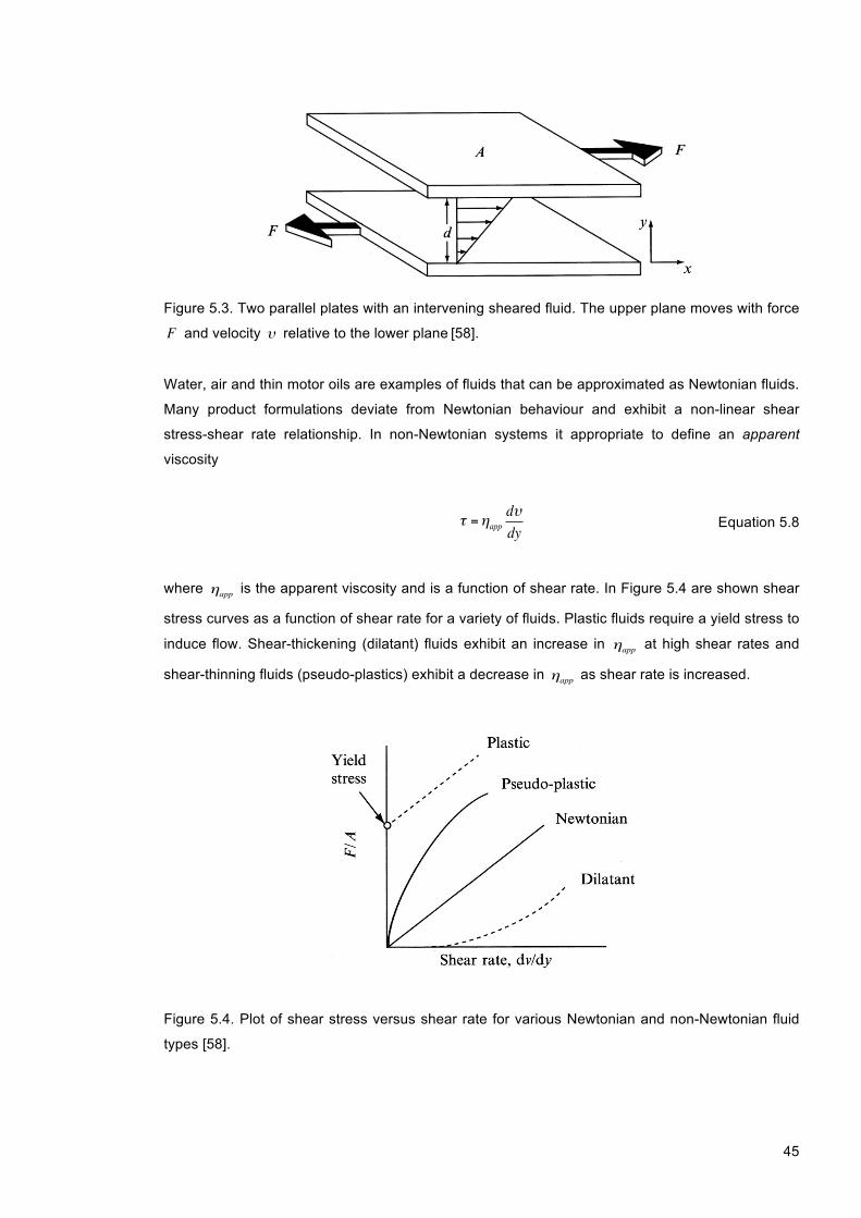
45

Figure 5.3. Two parallel plates with an intervening sheared fluid. The upper plane moves with force

F and velocity υ relative to the lower plane [58].

Water, air and thin motor oils are examples of fluids that can be approximated as Newtonian fluids.

Many product formulations deviate from Newtonian behaviour and exhibit a non-linear shear

stress-shear rate relationship. In non-Newtonian systems it appropriate to define an apparent

viscosity

τ =ηappdυdy

Equation 5.8

where ηapp is the apparent viscosity and is a function of shear rate. In Figure 5.4 are shown shear

stress curves as a function of shear rate for a variety of fluids. Plastic fluids require a yield stress to

induce flow. Shear-thickening (dilatant) fluids exhibit an increase in ηapp at high shear rates and

shear-thinning fluids (pseudo-plastics) exhibit a decrease in ηapp as shear rate is increased.

Figure 5.4. Plot of shear stress versus shear rate for various Newtonian and non-Newtonian fluid

types [58].

46

Bingham plastics are fluids that require a yield stress, σy to induce flow. At stresses less than σy the

particles can interact to form a rigid lattice. However, at stresses greater than σy the interactions

are overcome and flow ensues. Examples of Bingham plastics are toothpastes and most drilling

muds used for oil exploration.

Shear-thickening materials exhibit a non-linear increase in viscosity as a function of shear rate

where shear forces dominate repulsive inter-particle forces. At the molecular level, increasing

shear rate can move particles out of their equilibrium positions. As a consequence, inter-particle

jamming occurs and viscosity increases. Shear thickening behaviour depends on the volume

fraction of particles in a suspension. Higher particle volume fractions require lower shear rates to

induce dilatant behaviour. Another mechanism used to explain dilatency is hydroclustering, which

occurs when shearing of a particle suspension induces grouping of particles into irregular clusters.

The hydroclusters are believed to have extremely small separation distances, yielding a quasi-

incompressible transient structure. Furthermore, it is possible for hydroclusters to form via

molecular aggregation. Examples of dilatant fluids are Oobleck and silica in polyethylene glycol

mixtures [66].

Shear-thinning properties are commonly observed in surfactant solutions and are most relevant to

research conducted for this project. In Figure 5.5 are depicted the mechanisms responsible for

shear-thinning in dilute and concentrated surfactant systems.

Figure 5.5. Shear-thinning in dilute and concentrated surfactant systems [58]. D is the shear rate.

In dilute systems shear thinning occurs due to re-orientation of particles along the direction of

shear. The particles become aligned once the shear rate exceeds the rate of thermal re-orientation

47

of particles. In concentrated systems, shear thinning is observed when the shear rate exceeds the

rate of build-up of equilibrium macrostructures.

5.3.2 Thixotropy, Rheopexy and Viscoelasticity

Under constant shear rate conditions the viscosity of a complex fluid may exhibit time dependency.

Thixotropy is a common property of shear thinning fluids, in which the viscosity decreases as a

function of time. In surfactant systems, thixotropy occurs due to gradual re-orientation and

breakdown of aggregate structures. If the shear force is removed, aggregate structures reform and

viscosity gradually increases to an equilibrium value. A far less commonly observed property of

shear thickening fluids is rheopexy, in which fluid viscosity increases as a function of time.

Examples of rheopectic materials are some lubricants and semen [67, 68].

Viscoelastic materials exhibit both viscous and elastic properties. On subjecting an elastic material

to an external oscillatory stress, the shear stress peaks at maximum strain ( = ∂(x − X) ∂X where x

is final deformation length and X is initial length). Shear stress varies in phase with strain and the

phase shift between stress and strain, δ , is equal to 0°. For viscous liquids, the shear stress peaks

at maximum shear rate and therefore occurs at zero deformation. Shear stress is out of phase with

deformation and the phase shift δ is equal to 90°. Viscoelastic liquids exhibit some phase lag

between stress and strain, therefore 0° < δ < 90°. Viscoelastic materials are characterised by the

in phase and out of phase components of the modulus (stress to strain ratio).

Shear storage modulus G ' =σ 0

ε0

cosδ Equation 5.9

Shear loss modulus G '' =σ 0

ε0

sinδ Equation 5.10

where σ 0 is the shear stress and ε0 the shear strain. G ' is a measure of the elastic component of

energy stored and G '' is a measure of the viscous component of energy dissipated as heat.

5.4 X-ray Diffraction

X-ray diffraction (XRD) is often used to aid the identification of liquid crystal phases from

characteristic Bragg reflections of long-range order (>5 Å). XRD data generates information of

hydrocarbon chain order and distances between repeat structural units. Wide angle x-ray

scattering (WAXS) is used to obtain information such as head-group packing, whereas small angle

x-ray scattering (SAXS) is used to determine larger scale information, such as the distance

48

between partially ordered aggregates and bilayer thickness [69]. In XRD experiments the

wavelength is specific to the material of the x-ray tube (commonly Cu, Mo or Cr-Ka).

5.4.1 Introduction to X-rays

X-rays are a form of electromagnetic radiation of wavelength between 10-8 and 10-12 m and can be

generated using an x-ray tube, which uses high voltages to accelerate electrons from a high

temperature cathode. The high velocity electrons collide with the anode, creating x-rays. In x-ray

crystallography a copper target metal is common. Two of the mechanistic processes that generate

x-rays are

1. Fluorescence: During impact of a high-energy electron and an atom, an electron may be

ejected from the inner shell of the atom. Consequently, an electron from a higher energy orbital

fills the vacancy and a photon is emitted. The fluorescence process results in an emission

spectrum of x-rays at discrete wavelengths. The wavelength of photons emitted via discreet

are specific to the subject nuclei.

2. Bremsstrahlung: A type of radiation emitted by electrons as they are scattered by the strong

electric field of an atomic nucleus is known as Bremsstrahlung radiation. Bremsstrahlung x-

rays are characterised by a continuous spectrum and shift to higher frequencies when the

energy of incident electrons are increased.

Consider a sample material and an incident x-ray beam. The x-ray photons interact with electrons

in the atomic nuclei and a fraction of the photons are scattered as a spherical wave emanating

from the point source. If the wavelength of scattered x-rays remains constant, elastic scattering

(Rayleigh) has occurred and only momentum transfer takes place. X-ray diffraction measures the

intensities of elastically scattered photons as a function of scattering angle, which contains

information of the electron distribution in a material. In crystalline materials that possess long-range

periodic order, the diffraction pattern exhibits sharp interference peaks that characterise the

symmetry of distributed atoms. The diffraction pattern of a material is directly related to atomic

spacing and unit cell geometry.

5.4.2 Bragg’s Law

Diffraction of x-rays from a crystalline material is commonly described using Bragg’s law. The

theory treats crystals as a periodic build-up of lattice planes, such that each plane acts as a semi-

transparent mirror [70]. Bragg’s law states that when two scattered rays are in-phase they

constructively interfere to yield diffracted beams. When considering multiple lattice planes in a

crystal structure, the phase shift between the two beams (pathlength difference) must be

accounted for to ensure that beams transverse adjacently in parallel. In Figure 5.7 are shown two

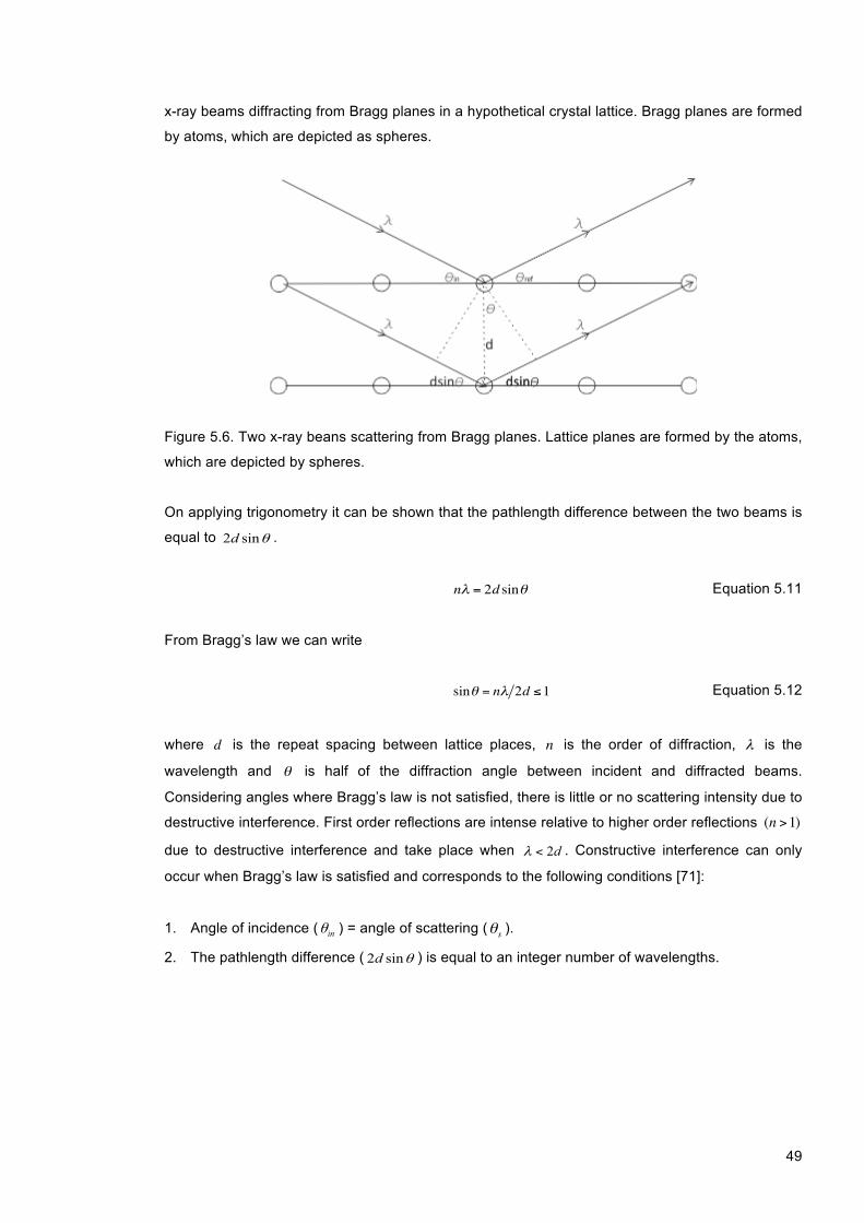
49

x-ray beams diffracting from Bragg planes in a hypothetical crystal lattice. Bragg planes are formed

by atoms, which are depicted as spheres.

Figure 5.6. Two x-ray beans scattering from Bragg planes. Lattice planes are formed by the atoms,

which are depicted by spheres.

On applying trigonometry it can be shown that the pathlength difference between the two beams is

equal to θsin2d .

nλ = 2d sinθ Equation 5.11

From Bragg’s law we can write

sinθ = nλ 2d ≤1 Equation 5.12

where d is the repeat spacing between lattice places, n is the order of diffraction, λ is the

wavelength and θ is half of the diffraction angle between incident and diffracted beams.

Considering angles where Bragg’s law is not satisfied, there is little or no scattering intensity due to

destructive interference. First order reflections are intense relative to higher order reflections (n >1)

due to destructive interference and take place when d2<λ . Constructive interference can only

occur when Bragg’s law is satisfied and corresponds to the following conditions [71]:

1. Angle of incidence ( inθ ) = angle of scattering (θs ).

2. The pathlength difference ( θsin2d ) is equal to an integer number of wavelengths.

50

5.4.3 Small Angle X-ray Scattering

SAXS experiments are usually conducted in the sub-1° regime for characterising systems with

large d spacing (nm-µm), such as liquid crystals, macromolecules, polymers and self-assembled

structures (e.g. zeolites). Technical challenges with SAXS are associated with the small angular

difference between the incident and scattered beam. Good signal to noise ratios are achieved via

the use of high quality collimating optics and beam stop positioning [72].

In liquid crystalline systems SAXS can be used to obtain information on aggregate ordering, size,

shape, intermolecular separation and spacing between bilayer structures. Our research focused on

utilising SAXS for characterising mesophases by determining intermolecular separation distances.

The area per molecule in a lamellar mesophase can be calculated from x-ray 0d (most intense

peak) spacings and the equations presented assume an infinite bilayer structure [73]. The moles of

surfactant in 1.0 g of sample may be calculated from

ms =Z

100S Equation 5.13

where sm is the number of moles of surfactant and Z is the concentration of surfactant (w/w %) of

molar mass S . The surfactant head groups have molar mass G and the hydrophobic chain molar

mass H . Consequently, S =G +H .

ZH =HS

Z100

Equation 5.14

Considering surfactant material ( 1=Z )

ZW =1− ZH Equation 5.15

where ZW and ZH are weight fractions of aqueous and hydrophobic regions respectively. The

volume fraction of the hydrophobic region, φH and the polar region φW are calculated using

φH =

Z HρH

Z HρH

− (1− Z H )ρW

Equation 5.16

φW =1−φH Equation 5.17

51

where ρW and ρH are mass densities of water and the bilayer respectively. For gel phases

9.0=Hρ kg m-3 and for the lamellar phase 8.0=Hρ kg m-3. ρW is assumed to occupy the value of

water (1.0 kg m-3). Assuming a lamellar phase, the thickness of hydrophobic and polar regions, dHand dW , are given by

dH = φHd0 Equation 5.18

dW = (1−φH )d0 Equation 5.19

The area per surfactant molecule a0 (m2), may be calculated using

a0 =2d0

ZWρW

+ZH

ρH

!

"#

$

%&1024

msN Equation 5.20

where N is Avogadro’s number (= 6.02214 × 1023 mol-1).

5.4.4 Wide Angle X-ray Scattering

Wide angle x-ray scattering is one of the most common experimental techniques used for structural

determination in materials possessing a high degree of short-range order. The technique is often

utilised in colloidal systems such as surfactant liquid crystals and polymeric materials. For our

research, WAXS was used to probe intra-aggregate surfactant separation distances and

differentiate between liquid crystal mesophases.

5.5 Dynamic Light Scattering

5.5.1 Correlation Function, Z-average Diameter and Polydispersity

Dynamic light scattering (DLS) is a non-invasive technique that is commonly used for

characterisation of micelle size and diffusion properties in surfactant solutions. DLS experiments

measure the intensity auto-correlation function C(t) = Agt2 +B , where A is an optical constant of

the instrument and B is a background constant. t is time and g is the first order autocorrelation

function. For monodisperse samples where the wavelength of light is far greater than the size of

the particle, the first order autocorrelation function g(t) is given by

g(t) = exp(−Dq2t) Equation 5.21

52

where q is the scattering vector ( q = 4πn0 sin(θ / 2) / λ , where θ is the scattering angle) [74]. DLS

is used to measure the translational diffusion coefficient of the particle D , which governs the delay

time for correlations in scattered light fluctuations. For monodisperse samples, D can be

calculated by fitting g(t) to an exponential decay as given in Equation 5.22. However for

polydispere solutions, each aggregate size contributes to the correlation function as given by

∑∑ −

=i ii

i iii

MtqDM

tg2

22 )exp()(

ρ

ρ Equation 5.22

which corresponds to a z-weighted average over all particle sizes of molecular weight Mi and

density ρi . Relating D to the correlation function is an ill-conditioned problem because different

distributions may yield the same measured value of g(t) . For mononodal particle distributions, a

way to overcome this problem is to use the cumulants expansion, which fits the natural logarithm of

the correlation function to a second order polynomial in the delay time.

224

2 )(2

)(ln zz DtqtDqtg δ+−= Equation 5.23

where the subscript “z” denotes the intensity based harmonic mean. The first order term in the

delay time relates to the z-average diffusion coefficient, whereas the second order term is

proportional to the variance in the z-average diffusion coefficient (smaller variance implies a thinner

size distribution). The z-average diffusion coefficient is regularly converted to hydrodynamic size,

which corresponds to a sphere with the same diffusion coefficient as the z-averaged diffusion

coefficient for the polydispersed sample.

z

BH D

Tkd

πη3= Equation 5.24

dH is the hydrodynamic diameter, kB is the Boltzmann constant, T is the thermodynamic

temperature and η is the solvent viscosity.

The polydispersity index is a measure of the width of a particle size distribution, and can be defined

as ( )2/ Hdσχ = , where σ is the standard deviation in dH . For monodisperse samples χ is equal

to zero, whereas values greater than 0.1 indicate a relatively broad size distribution.

A requirement for DLS is a minimum amount of background electrolyte to negate the electrostatic

repulsion between particles. Otherwise, the electrostatic repulsions induce a larger apparent

diffusion coefficient and thus a larger apparent particle size. A limitation of this technique is that

53

concentrated samples may not be studied as backscattering occurs, in which scattering information

is lost [5, 74, 75].

5.6 Static Light Scattering

Static light scattering measures light scattering intensity as a time-average value as a function of

scattering angle. Conversely, dynamic light scattering involves measuring the temporal variation in

scattering intensity, which is usually reported as an intensity auto-correlation function (Section

5.5.1) [76]. This section focuses on introducing a brief description of static light scattering, which is

frequently used to probe microstructure in colloidal systems. Applications are extensive and include

molecular weight determination, probing interparticle interactions and calculating radius of gyration.

For this research SLS was used to probe micelle growth kinetics by measuring photon scattering

intensity (count rate) as a function of time after mixing aqueous surfactant components.

5.6.1 Rayleigh Ratio and the Zimm Equation

Large molecules in solution scatter light due to thermal fluctuations in local concentration. To relate

scattered intensity caused by a particle to its properties, the excess scattering per unit volume and

scattering angle is normalised by the incident intensity. The corresponding excess Rayleigh ratio

(Rayleigh ratio of the sample minus that of the solvent) is expressed as [77]

R(θ ) = KMwP(θ )S(θ ) Equation 5.25

where K is the optical constant ( ANdcdnnK 40

22 /)(2 λπ= ), n is the refractive index, dn dc is the

specific refractive index increment, λ0 is the wavelength in a vacuum, NA is Avogadro’s number, c

is concentration (mol L-1), )(θR is the Rayleigh ratio and Mw is the molecular weight. P(θ ) and

S(θ ) are the particle form and structure factors at angle θ and allow for intra- and inter-particle

effects, respectively. The length scale over which light scattering is determined is characterised by

the scattering wave number q (Å-1).

⎟⎠

⎞⎜⎝

⎛=

2sin4 θ

λπnq Equation 5.26

When particle size is small relative to the wavelength of light, a simplified version of the Zimm

equation is valid [78]

...2)(1)( 2 ++= cAMP

RKcwθ

θ Equation 5.27

54

where A2 is the second virial coefficient. P(θ ) describes the angular variation in scattering

intensity and account for interparticle interference. Extrapolating to a 0° angle means the P(θ )

term tends to one. In micellar systems, the Mw term is apparent due to a broad size distribution.

The second virial coefficient describes whether the intraparticle interactions are attractive or

repulsive. Negative values correspond to attraction whereas positive values indicate attraction [79].

5.7 Nuclear Magnetic Resonance Spectroscopy

Nuclear magnetic resonance (NMR) spectroscopy is an extremely versatile technique that is

frequently used to probe solution dynamics and aggregation properties in micellar systems. The

variety of applications are extensive, and range from critical micelle concentration determination to

elucidating solution structure of microemulsions and ion binding [80]. In this section is presented a

brief overview of NMR with relevance to surfactant-based systems.

5.7.1 Spin Physics

Nuclear magnetic resonance occurs when the nuclei of atoms, possessing a property known as

spin, are placed in an external magnetic field and exposed to a radiofrequency pulse. Spin

describes the intrinsic angular momentum of a nucleus and is quantified by the spin quantum

number, I . The spin quantum number I is expressed in integral or half-integral values and the

total magnitude of spin angular momentum is h I(I +1) , where h is Planck’s reduced constant.

Since I is quantised, several discreet values of angular momentum exist and are defined by the

magnetic quantum number, m . For a given nuclei, m can take values from + I to – I in integer

steps, leading to a total of 2I +1 spin states. In addition, a spin-active nucleus has an associated

magnetic moment µ . The components of µ associated with different spin states are defined by

mµ / I , such that µ has 2I +1 components.

The magnetic moment and angular momentum behave as parallel or antiparallel vectors. The

relationship between µ and I is expressed by the gyromagnetic ratio γ :

γ =µhI

Equation 5.28

For a given nuclei immersed in a static magnetic field:

-‐ I = 0 : Absence of spin active nuclei means no local magnetic field is created (e.g. 12C, 16O).

The magnetic moment µ is equal to zero as the atomic charge is distributed evenly meaning

55

there is no circulation of nuclear charge. There is no electric field gradient eQ and is therefore

an isotropic electric field. Consequently, the nuclear electric quadrupole moment eQ = 0 .

-‐ I =1/ 2 : The nucleus spins as a spherical charged rigid body, inducing a magnetic field and a

single line peak is generated in the NMR spectrum (often split by dipolar coupling effects). A

circulation of nuclear charge leads to a magnetic moment ( µ ≠ 0 ), however as the charge is

distributed evenly around the spherical body, eQ = 0 .

-‐ I >1/ 2 : The nucleus spins as a non-spherical charged rigid body, creating a magnetic field

and the NMR spectrum exhibits multiple lines ( 2I ) as a consequence of quadrupolar splitting,

Δ . The uneven charge distribution in such nuclei results in an electric field gradient. Both µ

and eQ ≠ 0 . eQ > 0 for elongated rigid bodies (2H, 14N, …) and eQ < 0 for flattened rigid body

structures (17O, 35Cl, etc.).

5.7.2 Nuclear Energy Levels in a Magnetic Field

In the absence of an external magnetic field, all spin states are of equal energy. Application of an

external magnetic field of frequency B0 leads to the spin states occupying different energy values,

a process that forms the basis of NMR spectroscopy. For a Cartesian coordinate system with B0

aligned along the z-axis, the energy of a nucleus splits into 2I +1 orientations. The energy of a

nucleus with magnetic moment µ in field strength 0B is equal to −µzB0 , where µz is the

component of µ in the field direction. The energy of various spin states is −mµB0I−1 and the

separation between adjacent states is equal to −µB0I−1 . In Figure 5.7 are illustrated the splitting in

energy level for a spin active nuclei of I =1 [81].

Figure 5.7. (a) Nuclear spin energy of a single nucleus of I =1 plotted as a function of magnetic

field strength, B0 . (b) Alignment of magnetic vectors in relation to B0 .

56

Boltzmann statistics indicates that it is slightly more favourable for spins to align in the lowest

energy state, however alignment is opposed by thermal contributions, and thus temperature is a

parameter in the Boltzmann equation. Considering a spin active nuclei with I =1/ 2 and thus two

spin states, the population ratio between upper and lower spin states is given by

Pr =Nupper

Nlower

=1+ 2µB0kT

= exp(−ΔE / kT ) Equation 5.29

where Pr is the population ratio, Nupper is the population density of the upper spin state and Nlower

is the population density of the lower spin state. Signal intensity is dependent on the difference in

energy absorbed and emitted from the spins to make the transition between states.

Correspondingly, the signal is proportional to the population difference, Pd .

Pd = Nupper − Nlower =1−Nupper

Nlower

Equation 5.30

Thermal nuclear relaxation is required to achieve equilibrium distribution of nuclei between the

various spin states. Energy transfer among nuclei in different energy states and the surroundings

governs the process. Thermal nuclear relaxation is known as nuclear precession, and occurs about

the magnetic field axis at an angular velocity ω0 .

To induce a transition between spin states and perturb equilibrium spin populations, an external

rotating magnetic field at the Larmour frequency ν0 (= γB0 2π =ω0 2π )q must be applied. Two time

constants, T1 (spin-lattice) and T2 (spin-spin) are used to characterise the relaxation of nuclear

magnetisation back to equilibrium. Nuclear relaxation about B0 induces a periodic oscillating

voltage in radiofrequency coils surrounding the sample. The result is a time domain NMR signal,

from which may be derived the NMR spectrum in the frequency domain via Fourier transformation.

5.7.3 Spin-Lattice Relaxation

Nuclei within a sample undergo constant vibrational and rotational motion, which creates a

complex magnetic field known as the lattice field. The lattice field of nuclei in a low energy state

may interact with the lattice field of nuclei in a higher energy state, resulting in redistribution of

energy back to equilibrium. Energy gained by nuclei from exposure to a radiofrequency pulse may

increase the sample temperature due to an increase in thermal motion. Spin-lattice ( 1T ) relaxation

refers to time constant governing the process by which the spins dissipate energy gained from the

radiofrequency pulse back to the lattice, hence restoring thermal equilibrium. 1T relaxation occurs

along the magnetic field direction. Spin-lattice relaxation may be described by the Bloch equation

[82, 83]

57

MZ =M0 (1− 2exp(−τ /T1)) Equation 5.31

where MZ is the magnetisation vector in the z-direction, τ is the radiofrequency exposure time

and M0 is the equilibrium magnetisation vector in the z-direction. T1 may be defined as the time

required for the z-magnetisation to decay by a factor of 2e.

5.7.4 Spin-Spin Relaxation

The relaxation process involving transverse magnetisation is governed by spin-spin relaxation and

the time constant T2 . Converse to spin-lattice relaxation, spin-spin relaxation involves no energy

transfer and may be interpreted as destructive interference in the precessing magnetisation due to

loss of phase coherence. Nuclei lose phase coherence by exchanging spin and consequently the

phases of precessing spins randomise. The resultant magnetisation vector proceeds towards the z-

axis and collective macroscopic magnetisation in the xy plane decreases to zero. The equation

describing spin-spin relaxation is [82, 84]

Mxy =M0 exp(−τ /T2 ) Equation 5.32

where Mxy is the next magnetisation vector and M0 is the equilibrium magnetisation vector in the

xy plane. It is transverse relaxation that defines the decay of the time domain NMR signal and the

linewidth at half height of the frequency domain NMR signal, Δνobs . T2 is related to the linewidth at

half height by

T2 = (πΔνobs )−1 Equation 5.33

5.7.5 Nuclear Relaxation Mechanisms

In this section is a brief summary of the four main mechanisms contributing to spin-lattice and spin-

spin relaxation processes, assuming diamagnetic nuclei [85, 86].

Dipolar Relaxation: Two spin active nuclei are required for dipolar relaxation. A magnetic field is

induced by one spin on the other, and vice-versa. The interaction provides a pathway for energy

transfer between spins and the lattice. Essentially, the dipole-dipole interaction turns molecular

motion into an oscillating magnetic field that can cause spin state transitions.

Quadrupolar Relaxation: Describes the interaction between electric field gradients of quadrupolar

nuclei. This interaction does not occur for molecules at the centre of tetrahedral or octahedral

symmetry. Electric field gradients induce a torque on the quadrupolar nuclei. Tumbling of the

molecule can induce transitions between spin states and the effectiveness is dependent on the

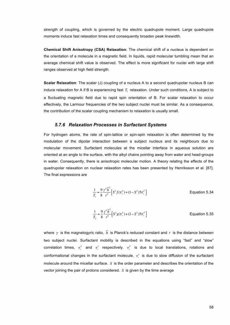
58

strength of coupling, which is governed by the electric quadrupole moment. Large quadrupole

moments induce fast relaxation times and consequently broaden peak linewidth.

Chemical Shift Anisotropy (CSA) Relaxation: The chemical shift of a nucleus is dependent on

the orientation of a molecule in a magnetic field. In liquids, rapid molecular tumbling mean that an

average chemical shift value is observed. The effect is more significant for nuclei with large shift

ranges observed at high field strength.

Scalar Relaxation: The scalar (J) coupling of a nucleus A to a second quadrupolar nucleus B can

induce relaxation for A if B is experiencing fast T1 relaxation. Under such conditions, A is subject to

a fluctuating magnetic field due to rapid spin orientation of B. For scalar relaxation to occur

effectively, the Larmour frequencies of the two subject nuclei must be similar. As a consequence,

the contribution of the scalar coupling mechanism to relaxation is usually small.

5.7.6 Relaxation Processes in Surfactant Systems

For hydrogen atoms, the rate of spin-lattice or spin-spin relaxation is often determined by the

modulation of the dipolar interaction between a subject nucleus and its neighbours due to

molecular movement. Surfactant molecules at the micellar interface in aqueous solution are

oriented at an angle to the surface, with the alkyl chains pointing away from water and head-groups

in water. Consequently, there is anisotropic molecular motion. A theory relating the effects of the

quadrupolar relaxation on nuclear relaxation rates has been presented by Henriksson et al. [87].

The final expressions are

1T1=98γ 4h

2

r6S2 f (τ c

S )+ (1− S2 )5τ cF"# $% Equation 5.34

1T2=98γ 4h

2

r6S2g(τ c

S )+ (1− S2 )5τ cF"# $% Equation 5.35

where γ is the magnetogyric ratio, h is Planck’s reduced constant and r is the distance between

two subject nuclei. Surfactant mobility is described in the equations using “fast” and “slow”

correlation times, τ cF and τ c

S respectively. τ cF is due to local translations, rotations and

conformational changes in the surfactant molecule. τ cS is due to slow diffusion of the surfactant

molecule around the micellar surface. S is the order parameter and describes the orientation of the

vector joining the pair of protons considered. S is given by the time average

59

S = 123cos2θDM −1 Equation 5.36

where θDM is the angle between the H-H vector and the normal to the micelle surface.

NMR spectra of micellar systems comprise an averaged contribution from micellar and monomeric

surfactant due to rapid exchange between the two species. Formation of large cylindrical micelles

results in increased time taken for a surfactant molecule to diffuse around the micelle surface [88-

90]. Consequently there is an associated “slow” correlation time ( τ cS , Section 5.7.6) in the

distribution of surfactant motions, which results in linewidth broadening of NMR signals [91].

Resonance lines in viscoelastic micellar solutions vary in width from 1 to over 100 Hz, depending

on surfactant concentration, temperature and the specific group inducing the signal. There is a

complex correlation between linewidth and viscosity. Non-viscous micellar solutions exhibit

linewidths of ~2 to 3 Hz, whereas the water resonance signal (residual protons in D2O) exhibits a

linewidth of less than 1 Hz, independent of macroscopic viscosity. In surfactant solutions the most

likely explanation for broad NMR linewidths is a distribution of micellar environments, where small

spherical micelles coexist with restricted mobility cylindrical micelles. Since a single NMR spectrum

is observed, the rate of monomer exchange between species must be rapid (>104 s-1) [89, 92, 93].

Small T2 values indicate that surfactant motion is anisotropic, with either a distribution of

correlation times (some > 10-8 s) or that non-averaged residual dipolar coupling contributes to the

observed T2 value. Small T2 values also occur when there is a degree of short-range order in the

system and the time taken for a molecule to experience all orientations is long compared to the

inverse of dipolar coupling. In our system it was assumed that the dipole coupling contribution to

T2 was averaged out by rapid monomer micelle exchange. Observed T2 values were assumed to

arise from a distribution of correlation times within the system [92] and were calculated as a

weighted average of T2 values from the individual ‘sites’ (independent proton resonance signals)

[94]

T2obs−1 = Pa (T2a )

−1

1

n

∑

Equation 5.37

Where the sum is over the types of independent sites a . aP and aT2 the fractional population and

spin-spin relaxation time at site a . Since an averaged value of T2 is observed and gives rise to a

single NMR spectrum, the monomer exchange rate between sites must be faster than the time

required to average spectra with different linewidths (~104 s-1).

60

6 Sodium Lauroyl Methyl Isethionate Production and Materials

6.1 Industrial Production of Sodium Lauroyl Methyl Isethionate

Sodium lauroyl methyl isethionate (SLMI; CMC (22.0 °C) = 1.5×10-3 mol kg-1, see Figure 6.1)) is

synthesised at industrial scale via a batch process and comprises a mixture of two isomers, 1 and

2 (9:1 w:w).

Figure 6.1. Surface tension of SLMI/water solutions plotted as a function of SLMI concentration.

Measurements were collected at 22.0 °C using the Wilhelmy plate technique and the CMC was

determined to be 1.5×10-3 mol kg-1. The reaction scheme for the SLMI production process is as

follows:

where dodecanoic acid (lauric acid, LA) and sodium methyl isethionate (SMI) are reagents.

Propylene glycol dilaurate (PGD) occurs as a side product and is not shown in the reaction

scheme. Heating LA and SMI under vacuum drives the reaction to completion. Excess LA is

20

30

40

50

60

70

80

0.01 0.1 1 10 100

Sur

face

Ten

sion

(m

N/m

)

Log(mmolal SLMI)

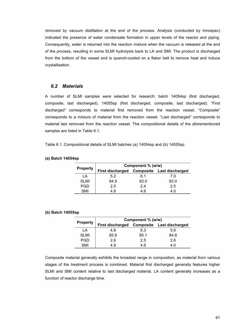
61

removed by vacuum distillation at the end of the process. Analysis (conducted by Innospec)

indicated the presence of water condensate formation in upper levels of the reactor and piping.

Consequently, water is returned into the reaction mixture when the vacuum is released at the end

of the process, resulting in some SLMI hydrolysis back to LA and SMI. The product is discharged

from the bottom of the vessel and is quench-cooled on a flaker belt to remove heat and induce

crystallisation.

6.2 Materials

A number of SLMI samples were selected for research: batch 14054sp (first discharged,

composite, last discharged), 14055sp (first discharged, composite, last discharged). “First

discharged” corresponds to material first removed from the reaction vessel. “Composite”

corresponds to a mixture of material from the reaction vessel. “Last discharged” corresponds to

material last removed from the reaction vessel. The compositional details of the aforementioned

samples are listed in Table 6.1.

Table 6.1. Compositional details of SLMI batches (a) 14054sp and (b) 14055sp.

(a) Batch 14054sp

Property Component % (w/w) First discharged Composite Last discharged

LA 5.2 6.1 7.0 SLMI 84.9 83.5 82.0 PGD 2.5 2.4 2.5 SMI 4.9 4.6 4.0

(b) Batch 14055sp

Property Component % (w/w) First discharged Composite Last discharged

LA 4.8 5.3 5.6 SLMI 85.6 85.1 84.8 PGD 2.6 2.5 2.6 SMI 4.9 4.6 4.0

Composite material generally exhibits the broadest range in composition, as material from various

stages of the treatment process is combined. Material first discharged generally features higher

SLMI and SMI content relative to last discharged material. LA content generally increases as a

function of reactor discharge time.

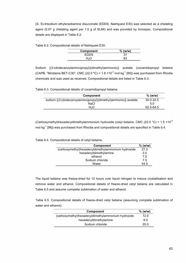
62

(S, S)-trisodium ethylenediamine disuccinate (EDDS, Natrlquest E30) was selected as a chelating

agent (0.07 g chelating agent per 1.0 g of SLMI) and was provided by Innospec. Compositional

details are displayed in Table 6.2.

Table 6.2. Compositional details of Natrlquest E30.

Component % (w/w) EDDS 37 H2O 63

Sodium {(3-(dodecanoylamino)propyl)(dimethyl)ammonio)} acetate (cocamidopropyl betaine

(CAPB, “Mirataine BET-C30”; CMC (22.0 °C) = 1.8 ×10-3 mol kg-1 [95]) was purchased from Rhodia

chemicals and was used as received. Compositional details are listed in Table 6.3.

Table 6.3. Compositional details of cocamidopropyl betaine.

Component % (w/w) sodium {(3-(dodecanoylamino)propyl)(dimethyl)ammonio)} acetate 30.0-32.5

NaCl 5.0 H2O 62.5-64.5

(Carboxymethyl)hexadecyldimethylammonium hydroxide (cetyl betaine, CMC (22.0 °C) = 1.5 ×10-5

mol kg-1 [96]) was purchased from Rhodia and compositional details are specified in Table 6.4.

Table 6.4. Compositional details of cetyl betaine.

Component % (w/w) (carboxymethyl)hexadecyldimethylammonium hydroxide 27.5

hexadecyldimethylamine 3.0 ethanol 7.5

Sodium chloride 7.5 Water 54.5

The liquid betaine was freeze-dried for 12 hours over liquid nitrogen to induce crystallisation and

remove water and ethanol. Compositional details of freeze-dried cetyl betaine are calculated in

Table 6.5 and assume complete sublimation of water and ethanol.

Table 6.5. Compositional details of freeze-dried cetyl betaine (assuming complete sublimation of

water and ethanol).

Component % (w/w) (carboxymethyl)hexadecyldimethylammonium hydroxide 72.0

hexadecyldimethylamine 8.0 Sodium chloride 20.0

63

Deuterium oxide (D2O) was provided by Sigma and used as received (99.9 % atom D).

Electrolytes were sourced from various suppliers: NaCl (>99 %, Fisher Scientific), NaSCN (>98 %,

Sigma), Na2HPO4 (>99 %, Sigma), NaNO3 (>99 %, Fluka), LiCl (99 %, Sigma), KCl (>99 %, Fluka),

and NH4Cl (>99 %, MP Biomedicals). All electrolytes were used as received.

Molecular structures of all research components (except salts) used for research are provided in

Table 6.6.

Table 6.6. Molecular structures of research components.

Component Molecular Structure

sodium lauroyl

methyl isethionate

9

9

S,S-trisodium

ethylenediamine

disuccinate

sodium {(3-

(dodecanoylamino)

propyl)(dimethyl)

ammonio}acetate

NH

64

(carboxymethyl)

Hexadecyldimethyl

ammonium

hydroxide 14

propylene glycol

dilaurate

sodium methyl

isethionate

dodecanoic acid

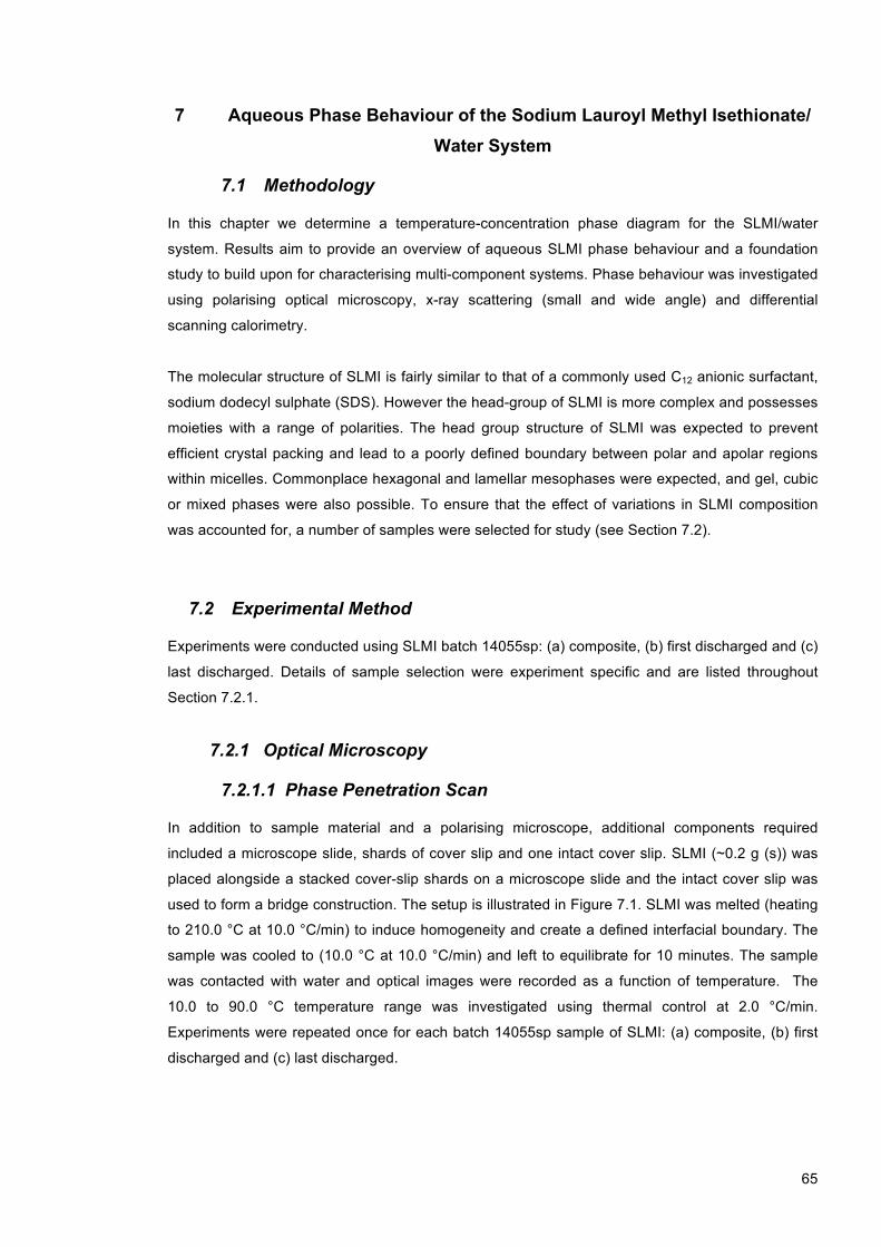
65

7 Aqueous Phase Behaviour of the Sodium Lauroyl Methyl Isethionate/ Water System

7.1 Methodology

In this chapter we determine a temperature-concentration phase diagram for the SLMI/water

system. Results aim to provide an overview of aqueous SLMI phase behaviour and a foundation

study to build upon for characterising multi-component systems. Phase behaviour was investigated

using polarising optical microscopy, x-ray scattering (small and wide angle) and differential

scanning calorimetry.

The molecular structure of SLMI is fairly similar to that of a commonly used C12 anionic surfactant,

sodium dodecyl sulphate (SDS). However the head-group of SLMI is more complex and possesses

moieties with a range of polarities. The head group structure of SLMI was expected to prevent

efficient crystal packing and lead to a poorly defined boundary between polar and apolar regions

within micelles. Commonplace hexagonal and lamellar mesophases were expected, and gel, cubic

or mixed phases were also possible. To ensure that the effect of variations in SLMI composition

was accounted for, a number of samples were selected for study (see Section 7.2).

7.2 Experimental Method

Experiments were conducted using SLMI batch 14055sp: (a) composite, (b) first discharged and (c)

last discharged. Details of sample selection were experiment specific and are listed throughout

Section 7.2.1.

7.2.1 Optical Microscopy

7.2.1.1 Phase Penetration Scan

In addition to sample material and a polarising microscope, additional components required

included a microscope slide, shards of cover slip and one intact cover slip. SLMI (~0.2 g (s)) was

placed alongside a stacked cover-slip shards on a microscope slide and the intact cover slip was

used to form a bridge construction. The setup is illustrated in Figure 7.1. SLMI was melted (heating

to 210.0 °C at 10.0 °C/min) to induce homogeneity and create a defined interfacial boundary. The

sample was cooled to (10.0 °C at 10.0 °C/min) and left to equilibrate for 10 minutes. The sample

was contacted with water and optical images were recorded as a function of temperature. The

10.0 to 90.0 °C temperature range was investigated using thermal control at 2.0 °C/min.

Experiments were repeated once for each batch 14055sp sample of SLMI: (a) composite, (b) first

discharged and (c) last discharged.

66

Figure 7.1. Phase penetration experimental setup. Mesophases develop in between the point of

solvent contact and the solid surfactant phase [97].

7.2.1.2 Optical Microscopy of Aqueous Samples

Optical microscopy was used to characterise aqueous SLMI/water samples of known

concentration. All glassware was washed using nitric acid (1.0 M) and Mili-Q water. SLMI/water

solutions ranging from 40.0 to 60.0 % (w/w) were prepared by diluting a SLMI/water stock solution

(60.0 % (w/w)) with Mili-Q water. Phase behaviour was observed as a function of temperature

(10.0 to 90.0 °C range) at a rate of 2.0 °C/min. Phase transitions were indicated by changes in

phase-specific optical characteristics, which are described in Section 3.2. Experiments were

performed using SLMI batch 14055sp: (a) composite, (b) first discharged and (c) last discharged.

7.2.1.3 Experimental Setup

Experiments were performed using a Jenaval polarising optical microscope fitted with Carl Zeiss

Axioplan Lens (objective of x10, x10 magnification). Images were recorded using a JVC KY-F55B

3-CCD camera. A Linkam LNP TMS 94 hot-stage and a liquid nitrogen dewar were coupled to the

microscope for thermal control (± 0.1°C). Linkam Linksys 32 software was used to control the hot-

stage and Image Pro Plus was used for exporting images to usable formats (tiff, jpeg, etc.).

7.2.2 Small Angle X-Ray Scattering

All glassware was washed using nitric acid (1.0 M) and Mili-Q water. 40.0 to 60.0 % (w/w)

SLMI/water (batch 14055sp composite) solutions were reused from Section 7.2.1. Samples were

heated to 40.0 °C in a beaker and slowly agitated using a magnetic stirrer. Samples were loaded

into Lindeman capillary tubes (1.0 mm diameter, quartz) and thermally sealed using a Bunsen

flame. The sample capillary was placed in the diffractometer sample holder. Scattering data was

collected from the 10 to 60 °C temperature range (equilibrated for 30 minutes at the desired

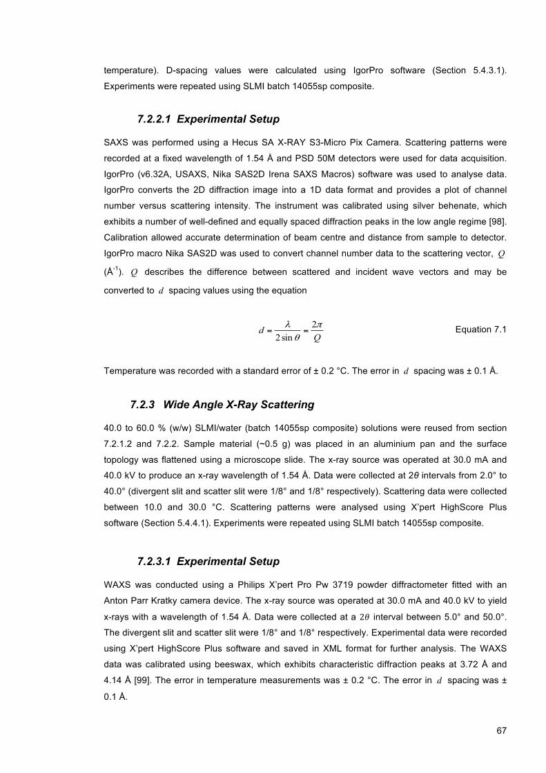
67

temperature). D-spacing values were calculated using IgorPro software (Section 5.4.3.1).

Experiments were repeated using SLMI batch 14055sp composite.


SAXS was performed using a Hecus SA X-RAY S3-Micro Pix Camera. Scattering patterns were

recorded at a fixed wavelength of 1.54 Å and PSD 50M detectors were used for data acquisition.

IgorPro (v6.32A, USAXS, Nika SAS2D Irena SAXS Macros) software was used to analyse data.

IgorPro converts the 2D diffraction image into a 1D data format and provides a plot of channel

number versus scattering intensity. The instrument was calibrated using silver behenate, which

exhibits a number of well-defined and equally spaced diffraction peaks in the low angle regime [98].

Calibration allowed accurate determination of beam centre and distance from sample to detector.

IgorPro macro Nika SAS2D was used to convert channel number data to the scattering vector, Q

(Å-1). Q describes the difference between scattered and incident wave vectors and may be

converted to d spacing values using the equation

Qd π

θλ 2sin2

== Equation 7.1

Temperature was recorded with a standard error of ± 0.2 °C. The error in d spacing was ± 0.1 Å.

7.2.3 Wide Angle X-Ray Scattering

40.0 to 60.0 % (w/w) SLMI/water (batch 14055sp composite) solutions were reused from section

7.2.1.2 and 7.2.2. Sample material (~0.5 g) was placed in an aluminium pan and the surface

topology was flattened using a microscope slide. The x-ray source was operated at 30.0 mA and

40.0 kV to produce an x-ray wavelength of 1.54 Å. Data were collected at 2θ intervals from 2.0° to

40.0° (divergent slit and scatter slit were 1/8° and 1/8° respectively). Scattering data were collected

between 10.0 and 30.0 °C. Scattering patterns were analysed using X’pert HighScore Plus

software (Section 5.4.4.1). Experiments were repeated using SLMI batch 14055sp composite.


WAXS was conducted using a Philips X’pert Pro Pw 3719 powder diffractometer fitted with an

Anton Parr Kratky camera device. The x-ray source was operated at 30.0 mA and 40.0 kV to yield

x-rays with a wavelength of 1.54 Å. Data were collected at a 2𝜃 interval between 5.0° and 50.0°.

The divergent slit and scatter slit were 1/8° and 1/8° respectively. Experimental data were recorded

using X’pert HighScore Plus software and saved in XML format for further analysis. The WAXS

data was calibrated using beeswax, which exhibits characteristic diffraction peaks at 3.72 Å and

4.14 Å [99]. The error in temperature measurements was ± 0.2 °C. The error in d spacing was ±

0.1 Å.

68

7.2.4 Differential Scanning Calorimetry

All glassware was washed using nitric acid (1.0 M) and Mili-Q water. 40.0 to 60.0 % (w/w)

SLMI/water solutions were reused from section 7.2.1.2, 7.2.2 and 7.2.3. Sample material (~10 mg)

were placed into aluminium pans and sealed by compression. The sample pans were transferred

to the DSC device. Samples were equilibrated at 30.0 °C for 10 minutes. Samples were cooled to

0.0 °C at a rate of 2.0 °C/min. Thermograms were interpreted and analysed using Perkin-Elmer

Pyris v11 software (Section 5.2.2). Experiments were repeated using SLMI batch 14055sp (a)

composite, (b) first discharged and (c) last discharged.


DSC experiments were conducted using a Perkin-Elmer Diamond instrument. Using indium, the

thermogram (melting onset temperature (Tmelt = 156.6 °C)) and heat flow (area under the peak (

ΔH fusion = 28.45 Jg-1)) were calibrated. Perkin-Elmer Pyris v11 software was used for analysis. Data

extracted from DSC thermograms included phase transition onset temperatures and transition

enthalpies. The phase transition onset temperature was derived from the intersection of a linear

extrapolation of the transition peak with the baseline. Phase transition enthalpies were calculated

from the area under the peak from first and last departures from the baseline. The error in peak

temperature was ± 0.3 °C and the error in enthalpy was ± 0.5 Jg-1.

69

7.3 Results and Discussion

7.3.1 Phase Characterisation – Optical Microscopy

Polarised optical images of a SLMI/water penetration scan across the 10.0 to 90.0 °C temperature

range are shown in Figure 7.2. In total, four separate phases were identified. Phase assignments

were delineated using polarised optical images (Figure 7.3) in combination with x-ray experiments

conducted on samples of known concentration (Section 7.3.2 and 7.3.3). The least concentrated

phase is isotropic micellar ( 1L ); next is a two-phase 1Ha L+L region (identified by observing phase

separation in samples); the penultimate phase is lamellar with defects HaL and the final phase was

crystal.

12 27 45 53

60 70 80 90

Temperature °C

Figure 7.2. Phase penetration scan of SLMI (14055sp composite) by water across the 10.0 to 90.0

°C temperature range. From left to right the phase assignments in each image are crystal; HaL ;

1Ha L+L 1L . The red magnification line represents 100 µm.

Optical textures remain similar on increasing temperature, indicating that phase behaviour is fairly

insensitive to temperature across the experimental range. Such behaviour is often observed in

aqueous ionic surfactant systems, as ionic head-group-water interactions exhibit weak temperature

dependence [6, 100]. Only at temperatures above ~80 °C were slight changes in optical texture

observed due to evaporation of water.

Polarised optical micrographs of SLMI/water samples at known concentrations were recorded as a

function of temperature and are presented in Figure 7.3. Analysis of the data enabled qualitative

determination of the position of phase boundary locations and examination of optical textures in

greater detail. The single-phase LaH region was distinguished from the two-phase La

H+L1 region by

70

visual observation of samples in sealed glass containers. On heating SLMI/water samples (46.0,

48.0, 50.0 % (w/w)) the phase behaviour remained fairly insensitive with respect to changes in

temperature. The exact position of the LaH+L1 - La

H phase boundary was only approximately located

from visual observations.

SLMI

46.0 % (w/w)

LaH+L1

28.0 °C

LaH+L1

70.0 °C

SLMI

53.0 % (w/w)

LaH

26.0 °C

LaH+L1

77.0 °C

SLMI

55.0 % (w/w)

LaH

30.0 °C

LaH

75.0 °C

SLMI

56.0 % (w/w)

crystal + L1

25.0 °C

crystal + L1

73.0 °C

Figure 7.3. Polarised optical images of SLMI/water (14055sp composite) samples. The red

magnification bar represents 100 µm.

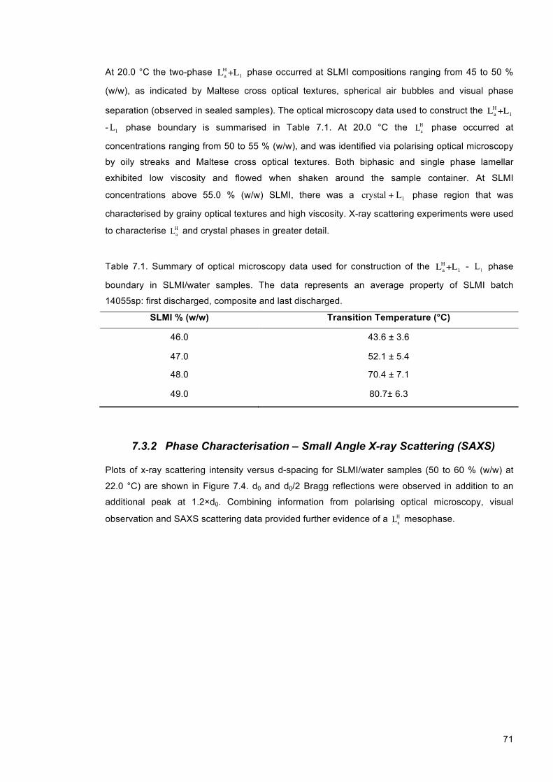
71

At 20.0 °C the two-phase LaH+L1 phase occurred at SLMI compositions ranging from 45 to 50 %

(w/w), as indicated by Maltese cross optical textures, spherical air bubbles and visual phase

separation (observed in sealed samples). The optical microscopy data used to construct the LaH+L1

- L1 phase boundary is summarised in Table 7.1. At 20.0 °C the LaH phase occurred at

concentrations ranging from 50 to 55 % (w/w), and was identified via polarising optical microscopy

by oily streaks and Maltese cross optical textures. Both biphasic and single phase lamellar

exhibited low viscosity and flowed when shaken around the sample container. At SLMI

concentrations above 55.0 % (w/w) SLMI, there was a crystal + L1 phase region that was

characterised by grainy optical textures and high viscosity. X-ray scattering experiments were used

to characterise LaH and crystal phases in greater detail.

Table 7.1. Summary of optical microscopy data used for construction of the LaH+L1 - 1L phase

boundary in SLMI/water samples. The data represents an average property of SLMI batch

14055sp: first discharged, composite and last discharged.

SLMI % (w/w) Transition Temperature (°C)

46.0 43.6 ± 3.6

47.0 52.1 ± 5.4

48.0 70.4 ± 7.1

49.0 80.7± 6.3

7.3.2 Phase Characterisation – Small Angle X-ray Scattering (SAXS)

Plots of x-ray scattering intensity versus d-spacing for SLMI/water samples (50 to 60 % (w/w) at

22.0 °C) are shown in Figure 7.4. d0 and d0/2 Bragg reflections were observed in addition to an

additional peak at 1.2×d0. Combining information from polarising optical microscopy, visual

observation and SAXS scattering data provided further evidence of a LaH

mesophase.

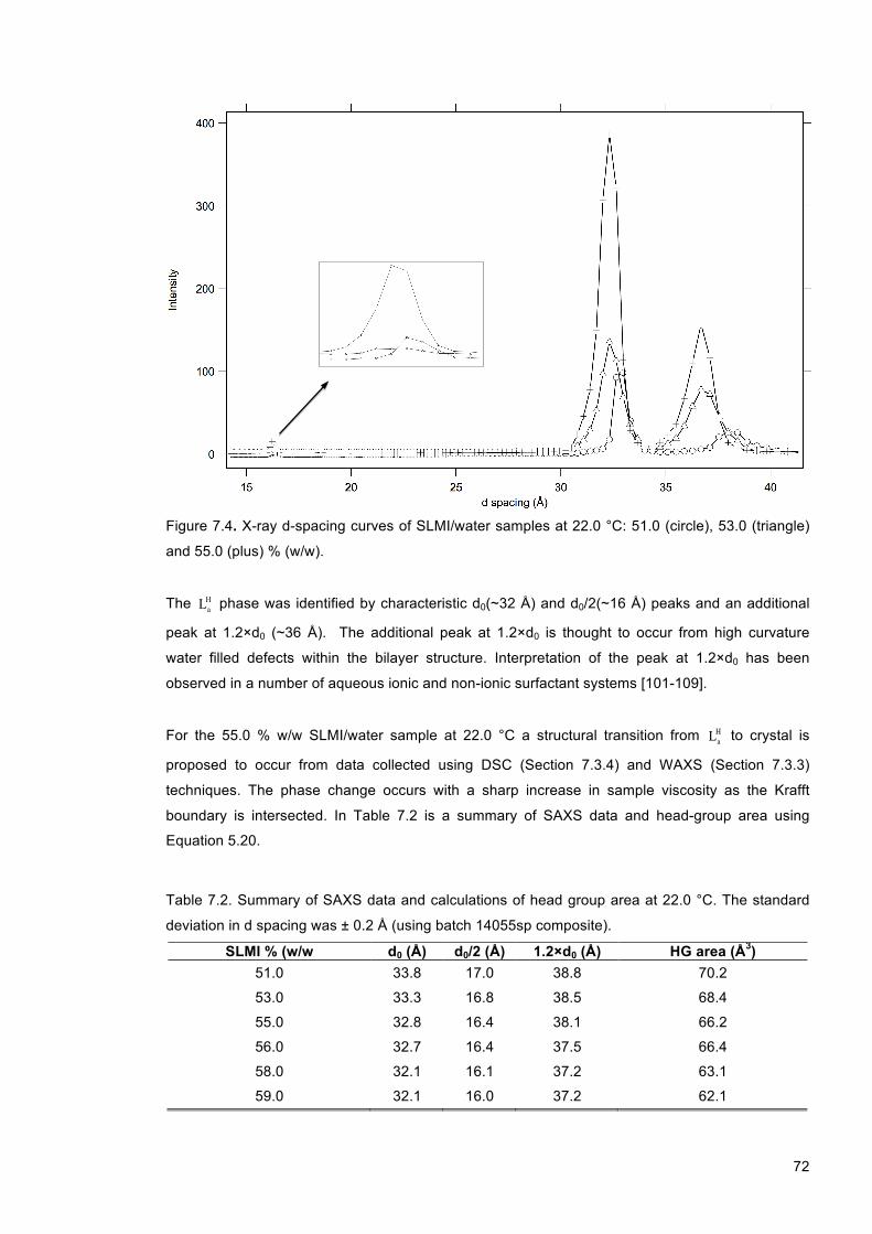
72

Figure 7.4. X-ray d-spacing curves of SLMI/water samples at 22.0 °C: 51.0 (circle), 53.0 (triangle)

and 55.0 (plus) % (w/w).

The LaH phase was identified by characteristic d0(~32 Å) and d0/2(~16 Å) peaks and an additional

peak at 1.2×d0 (~36 Å). The additional peak at 1.2×d0 is thought to occur from high curvature

water filled defects within the bilayer structure. Interpretation of the peak at 1.2×d0 has been

observed in a number of aqueous ionic and non-ionic surfactant systems [101-109].

For the 55.0 % w/w SLMI/water sample at 22.0 °C a structural transition from LaH to crystal is

proposed to occur from data collected using DSC (Section 7.3.4) and WAXS (Section 7.3.3)

techniques. The phase change occurs with a sharp increase in sample viscosity as the Krafft

boundary is intersected. In Table 7.2 is a summary of SAXS data and head-group area using

Equation 5.20.

Table 7.2. Summary of SAXS data and calculations of head group area at 22.0 °C. The standard

deviation in d spacing was ± 0.2 Å (using batch 14055sp composite).

SLMI % (w/w d0 (Å) d0/2 (Å) 1.2×d0 (Å) HG area (Å3) 51.0 33.8 17.0 38.8 70.2

53.0 33.3 16.8 38.5 68.4

55.0 32.8 16.4 38.1 66.2

56.0 32.7 16.4 37.5 66.4

58.0 32.1 16.1 37.2 63.1

59.0 32.1 16.0 37.2 62.1

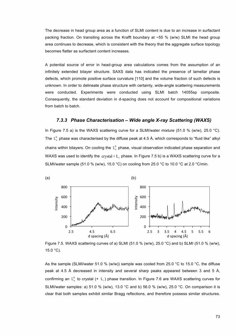
73

The decrease in head group area as a function of SLMI content is due to an increase in surfactant

packing fraction. On transiting across the Krafft boundary at ~55 % (w/w) SLMI the head group

area continues to decrease, which is consistent with the theory that the aggregate surface topology

becomes flatter as surfactant content increases.

A potential source of error in head-group area calculations comes from the assumption of an

infinitely extended bilayer structure. SAXS data has indicated the presence of lamellar phase

defects, which promote positive surface curvature [110] and the volume fraction of such defects is

unknown. In order to delineate phase structure with certainty, wide-angle scattering measurements

were conducted. Experiments were conducted using SLMI batch 14055sp composite.

Consequently, the standard deviation in d-spacing does not account for compositional variations

from batch to batch.

7.3.3 Phase Characterisation – Wide angle X-ray Scattering (WAXS)

In Figure 7.5 a) is the WAXS scattering curve for a SLMI/water mixture (51.0 % (w/w), 25.0 °C).

The HαL phase was characterised by the diffuse peak at 4.5 Å, which corresponds to “fluid like” alkyl

chains within bilayers. On cooling the HαL phase, visual observation indicated phase separation and

WAXS was used to identify the 1L + crystal phase. In Figure 7.5 b) is a WAXS scattering curve for a

SLMI/water sample (51.0 % (w/w), 15.0 °C) on cooling from 25.0 °C to 10.0 °C at 2.0 °C/min.

(a) (b)

Figure 7.5. WAXS scattering curves of a) SLMI (51.0 % (w/w), 25.0 °C) and b) SLMI (51.0 % (w/w),

15.0 °C).

As the sample (SLMI/water 51.0 % (w/w)) sample was cooled from 25.0 °C to 15.0 °C, the diffuse

peak at 4.5 Å decreased in intensity and several sharp peaks appeared between 3 and 5 Å,

confirming an HαL to crystal (+ 1L ) phase transition. In Figure 7.6 are WAXS scattering curves for

SLMI/water samples: a) 51.0 % (w/w), 13.0 °C and b) 56.0 % (w/w), 25.0 °C. On comparison it is

clear that both samples exhibit similar Bragg reflections, and therefore possess similar structures.

0

200

400

600

800

2.5 4.5 6.5

Intensity

d spacing (Å)

0

200

400

600

800

2.5 3 3.5 4 4.5 5 5.5 6

Intensity

d spacing (Å)

74

In addition, samples is Figure 7.6 possess higher degrees in crystallinity, as reflected by the

relatively larger signal intensity.

(a) (b)

Figure 7.6. WAXS scattering curves of SLMI/water samples using batch 14055sp composite: a)

51.0 % (w/w), 13.0 °C and b) 56.0 % (w/w), 25.0 °C. The appearance of multiple sharp peaks in b)

indicates the transition to a crystal phase.

The WAXS curves in Figures 7.5 and 7.6 confirm that intersection of the Krafft boundary occurs on

increasing SLMI concentration and cooling HαL samples. WAXS results are consistent with optical

microscopy data.

7.3.4 Lamellar - Crystal + Isotropic Phase Boundary Determination: Differential Scanning Calorimetry

DSC was used to determine phase transition onset temperatures and transition enthalpies on

cooling SLMI/water samples from LaH to crystal + L1 phase regions. Data were used to construct the

Krafft boundary, which is plotted in the phase diagram in Figure 7.8. Since the purpose of the

experiment was to determine the cooling transition temperature of the LaH

phase, only cooling

scans were utilised. DSC cooling traces of SLMI/water samples (40.0 to 60.0 % (w/w)) are shown

in Figure 7.7. 40.0 % (w/w) SLMI/water L1 samples exhibited no phase change on cooling. Several

SLMI/water samples in the L1 region were tested and similarly exhibited no phase change.

SLMI/water LaH samples (40.0, 51.0, 53.0 and 55.0 % (w/w)) exhibited an endothermic peak

(indicated by the stars on plots in Figure 7.7) indicative of first order phase transition. Phase

transition onset temperature increased with surfactant concentration.

0

1000

2000

3000

4000

5000

6000

2.5 3 3.5 4 4.5 5 5.5 6

Intensity

d spacing (Å)

0

2000

4000

6000

8000

10000

12000

2.5 3 3.5 4 4.5 5 5.5 6

Intensity

d spacing (Å)

75

(a) (b)

(c) (d)

Figure 7.7. DSC curves of SLMI/water (14055sp composite) samples at a) 40.0 %, b) 51.0 %, c)

53.0 % and d) 55.0 % (w/w).

HaL phase samples exhibited an endothermic peak on cooling. The magnitude of enthalpy change

(~15 kJ/mol) supports previous evidence suggesting a LaH to crystal phase transition. In Table 7.3 is

a summary of the DSC data collected.

Table 7.3. DSC cooling data of SLMI/water LaH phase samples. Enthalpy and transition temperature

represents an average property using SLMI batch 14055sp: first discharged, composite and last

discharged.

SLMI % (w/w) Enthalpy (kJ/mol) Transition Temperature (°C) 52.0 15.4 ± 2.4 17.5 ± 3.4 54.0 15.5 ± 5.7 23.7 ± 5.7 56.0 17.7 ± 3.4 27.0 ± 4.4

-‐4

-‐3

-‐2

-‐1

0

1

2 0 5 10 15 20 25 30

Heat Flow (m

W)

Temperature (°C)

-‐4 -‐3.5 -‐3

-‐2.5 -‐2

-‐1.5 -‐1

-‐0.5 0

0 5 10 15 20 25 30

Heat Flow (m

W)

Temperature (°C)

-4

-3.5

-3

-2.5

-2

-1.5

-1

-0.5

0 0 5 10 15 20 25 30

Hea

t Flo

w (m

W)

Temperature (°C)

-4

-3.5

-3

-2.5

-2

-1.5

-1

-0.5

0 0 5 10 15 20 25 30

Hea

t Flo

w (m

W)

Temperature (°C)

76

The time required for crystallisation to occur was dependent on sample concentration. Mesophase

samples crystallised within minutes, whereas isotropic samples only exhibited precipitation when

stored at low temperatures for timescales several orders of magnitude larger (weeks-months).

Consequently, L1 phase precipitation was not indicated on the phase diagram.

7.3.5 Lamellar + Isotropic - Crystal + Isotropic Phase Boundary Determination: Visual Identification

The LaH+L1 - crystal + L1 phase boundary was determined by visual observation using a

temperature controlled water bath (Clifton NE5D) and SLMI/water samples in sealed glass vials.

On cooling LaH+L1 SLMI/water samples (46.0 and 48.0 % (w/w)) at 0.5 °C/min to below the

transition temperature, a crystalline material separated. Experiments were repeated using SLMI

batch 14055sp (a) composite, (b) first discharged and (c) last discharged. A summary of the data

is presented in Table 7.4.

Table 7.4. Data collected for determining the LaH+L1 -

1L + crystal phase boundary by visual

observation, with aid of a temperature controlled water bath. Transition temperature represents an

average property using SLMI batch 14055sp: first discharged, composite and last discharged.

SLMI % (w/w) Transition Temperature (°C) 46.0 15.4 ± 3.2 48.0 15.5 ± 4.1

7.3.1 Sodium Lauroyl Methyl Isethionate/ Water Phase Diagram

Data collected throughout this Chapter was used to construct a temperature-composition phase

diagram, which is presented in Figure 7.8. The L1 phase was the lowest concentration phase and

preceded mesophase formation. A biphasic LaH+L1 phase region was observed and transitioned to

a LaH phase with increasing SLMI concentration. A crystal + L1 phase was also discovered.

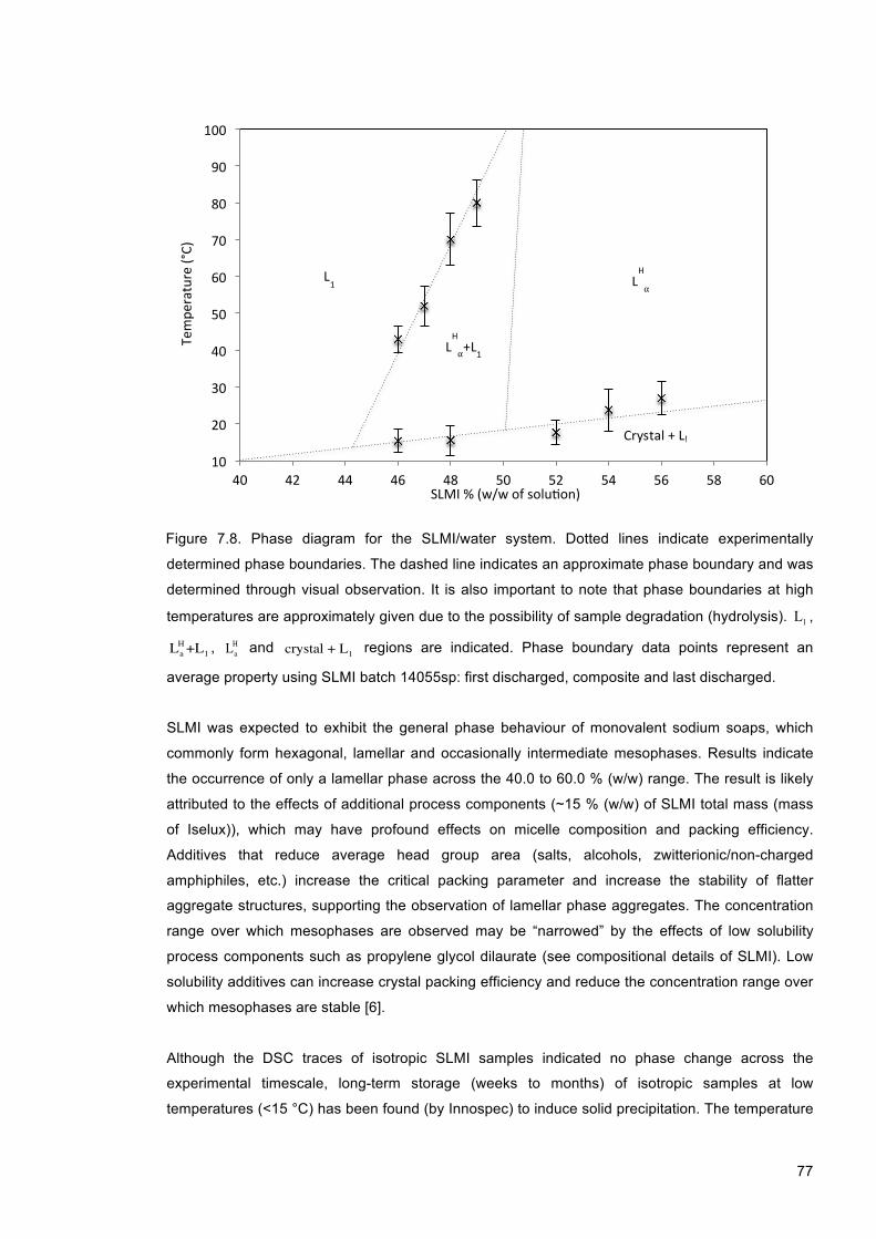
77

Figure 7.8. Phase diagram for the SLMI/water system. Dotted lines indicate experimentally

determined phase boundaries. The dashed line indicates an approximate phase boundary and was

determined through visual observation. It is also important to note that phase boundaries at high

temperatures are approximately given due to the possibility of sample degradation (hydrolysis). L1 ,

LaH+L1 , La

H and crystal + L1 regions are indicated. Phase boundary data points represent an

average property using SLMI batch 14055sp: first discharged, composite and last discharged.

SLMI was expected to exhibit the general phase behaviour of monovalent sodium soaps, which

commonly form hexagonal, lamellar and occasionally intermediate mesophases. Results indicate

the occurrence of only a lamellar phase across the 40.0 to 60.0 % (w/w) range. The result is likely

attributed to the effects of additional process components (~15 % (w/w) of SLMI total mass (mass

of Iselux)), which may have profound effects on micelle composition and packing efficiency.

Additives that reduce average head group area (salts, alcohols, zwitterionic/non-charged

amphiphiles, etc.) increase the critical packing parameter and increase the stability of flatter

aggregate structures, supporting the observation of lamellar phase aggregates. The concentration

range over which mesophases are observed may be “narrowed” by the effects of low solubility

process components such as propylene glycol dilaurate (see compositional details of SLMI). Low

solubility additives can increase crystal packing efficiency and reduce the concentration range over

which mesophases are stable [6].

Although the DSC traces of isotropic SLMI samples indicated no phase change across the

experimental timescale, long-term storage (weeks to months) of isotropic samples at low

temperatures (<15 °C) has been found (by Innospec) to induce solid precipitation. The temperature

10

20

30

40

50

60

70

80

90

100

40 42 44 46 48 50 52 54 56 58 60

Tempe

rature (°C)

SLMI % (w/w of soluOon)

LH

α L1

LH

α+L1

Crystal + L!

78

stability of SLMI mesophases presents a potential storage problem for distributors (samples may

be warehoused in winter season) and is an area that requires further attention. Whilst DSC

experiments were conducted at a rate of 2.0 °C/min, it is possible that subtleties in phase behavior

were missed. Kekicheff studied the sodium dodecyl sulfate/water system and discovered that a

cooling rate of 0.1 °C per minute was required to distinguish peak separation [111].

SAXS and WAXS analysis elucidated the lamellar phase, which is thought to contain water-filled

defects within the bilayer structure. Defects are often in the form of either dislocation loops, which

have been extensively investigated by Allain [112], or thermodynamically stable defects within a

highly curved bilayer [113]. The large head group area of SLMI is thought to promote a positively

curved aggregate geometry, and thus the latter defect structure is most likely to occur from

minimizing free energy in the system. The conventional lamellar phase without defects satisfies

global aggregate packing requirements, however there is a free energy penalty for packing the

molecules into an extended planar bilayer with zero curvature; water filled defect formation allows

surfactants with bulky head groups such as SLMI to retain positively curvature [109].

The phase diagram indicates that the phase rule is disobeyed for a multi-component system in the

crystal + L1 phase region. The result may possibly be attributed to the presence of additional

process components such as propylene glycol dilaurate, which act as additional components and

increase the number of degrees of freedom in the system. Formation of the crystal + L1 phase

region is commonly observed on intersecting the Krafft boundary and has been reported for a

multitude of surfactant systems [11].

7.4 Conclusions and Future Work

Our results were combined to produce a phase diagram of the SLMI/water system. Optical

microscopy and x-ray diffraction studies facilitated mesophase and crystal phase identification.

Differential scanning calorimetry and visual experiments enabled phase boundary determination.

The lamellar phases with defects dominated mesophase behaviour and spanned the 46.0 to 60.0

% (w/w) SLMI compositional range. Absence of a hexagonal phase, which is often observed in

similar systems, was attributed to the bulky head-group structure of SLMI, which is likely to prevent

formation of long cylindrical pre-hexagonal phase micelles. Cooling of the lamellar phases reduced

surfactant solubility and induced Krafft precipitation into a crystalline + water phase.

Our results provide a foundation for future experiments on determining the effects on SLMI phase

behaviour of additives such as fragrances, secondary surfactants, polymers and electrolytes.

Surface-active molecules that reduce hydrophobic chain packing efficiency (branches/double

bonded surfactants, alcohols) are expected to increase mesophase solubility and shift the Krafft

boundary to lower temperatures. Such molecules may broaden mesophase regions and an

understanding of their effects will be valuable to formulation scientists.

79

8 Rheological Performance Properties in Sodium Lauroyl Methyl Isethionate/ {(3-Dodecanoylamino)propyl(dimethyl)amino}acetate/ Water

Mixtures and the Effects of Process Components

8.1 Thickening in Surfactant Mixtures

SLMI has applications in personal care products such as shampoos, shower gels and facial

cleansers. Highly viscous formulations are desirable for ease of application and luxury. Innospec

has experienced variable viscosities in SLMI formulations. The viscosity of a formulation is

dependent on the concentration of process components, which may occur as reaction side-

products and/or unreacted reagent. The effects on viscosity of a standard formulation induced by

process components and variable reactor discharge times have been investigated via doping

experiments.

Shampoo and shower gel products incorporate thickening agents such as electrolytes and

secondary surfactants. Ionic surfactants are often combined with secondary surfactants

(zwitterionic/non-ionic/cationic) to increase viscosity, boost foam stability and reduce the CMC of

the mixture. For ionic surfactants in aqueous solution, aggregation initially leads to formation of

small micellar structures. Electrostatic repulsion between charged head-groups induces positive

curvature at the micelle surface. Addition of a secondary surfactant reduces the magnitude of

electrostatic surface repulsion and decreases the average head group area. Continual reduction in

micelle surface head group area eventually induces a micelle shape transition to a lower curvature

structure (see Section 2.5). Shape transitions from globular to rod micelles lead to an increase in

viscosity [114].

Electrolytes such as sodium chloride are frequently used to thicken surfactant product formulations.

Sodium chloride is the most commonly used thickening agent due to its cheapness and availability

[115-119]. Electrostatic head-group repulsion within micelles is reduced as ionic strength is

increased, resulting in a decrease in the effective head group area. Once ionic strength is high

enough to negate electrostatic interactions, further electrolyte addition results in progressive

“dehydration” of the micelle surface [120, 121]. Surface dehydration decreases the head group

area and consequently increases solution viscosity. Subsequent addition of salt induces break-up

of long rod micelles into smaller disc geometries and a corresponding decrease in viscosity follows.

It is widely understood that formulation viscosity peaks when the largest dimension of rod micelles

reaches maximum size. Formulation scientists use a combination of surfactants, salts and other

components to tune rheological properties [6].

Once a suitable starting formulation is identified, additional components such as fragrances and

foam boosters may be added. Once a based formulation is prepared, electrolyte may be added to

further increase formulation viscosity. The response of a particular formulation to added salt is

gauged using a “salt thickening curve”, which plots solution viscosity as a function of added salt. If

80

the salt thickening profile does not meet the required level, the base formulation needs to be

adjusted.

8.2 Methodology

8.2.1 Effects on Rheological Performance Caused by Variable Discharge Time

In Section 6.1 it was mentioned that at the end of the production process, water release induces

hydrolysis of SLMI into SMI and LA. The time taken to discharge the product material from the

reactor affects the extent of hydrolysis and therefore influences final composition. Hydrolysis is

more advanced at increased discharge times, as the material is subjected to high temperature for a

longer period of time. The effects of variable reactor discharge time were determined by conducting

viscosity measurements on a base formulation (see Section 8.2.1) using two separate batches of

SLMI, each containing markedly different levels of process component (Section 8.3.1). For each

batch, three samples were analysed corresponding to first, middle and last discharged positions

along the treatment process. Salt-thickening curves were determined and examined along with the

compositional data. The objective of the experiment was to determine a qualitative relationship

between formulation viscosity and reactor discharge time.

8.2.2 Effects of Process Components

The effects on formulation viscosity induced by the three most abundant (w/w % of Iselux) process

components were determined. Experiments were designed to isolate the effect on viscosity of the

component studied. Salt-thickening curves were constructed for a standard base formulation (see

Section 8.3.2) at incremental concentrations of process components. Experimental results were

analysed by considering molecular effects on micelle geometry.


8.3.1 Effects on Rheological Performance Caused by Variable Discharge Time

Glassware was washed with nitric acid (1.0 M) and Mili-Q water. Stock solutions were prepared

using two SLMI batches (batch 15054sp (last discharged) and batch 14055sp (composite)).

Compositional details are listed in Table 8.1.

81

Table 8.1. Compositional details of stock solution.

Component % (w/w) SLMI 10.00 CAPB 5.00

Natrlquest 0.92 Water 84.08

Stock solutions were poured into glass sample vials and NaCl was added to yield compositions

ranging from 0.0 to 2.0 % (0.2 % increments). Samples were left to equilibrate at room temperature

for two weeks. Sample viscosities were measured and salt thickening curves constructed (Section

8.3.4).

8.3.2 Effects of Process Components

Glassware was washed with nitric acid (1.0 M) and Mili-Q water. Stock solutions were prepared

using two batches of SLMI (batch 15054sp (last discharged) and batch 14055sp (composite)) at

incremental concentrations of each process component (propylene glycol dilaurate (PGD), sodium

methyl isethionate (SMI) and lauric acid (LA)). Compositional details are listed in Table 8.2.

Table 8.2. Compositional details of stock solutions. x was manually doped to yield process

component concentrations at 150 % and 200 % (w/w) of the standard process component

concentration in the base formulation.

(a)

Component % (w/w) SLMI 10 CAPB 5

Natrlquest 0.92 PGD x Water 84.08 - x

Where x = 0.00, 0.22 and 0.44.

(b)


Natrlquest 0.92 SMI x

Water 84.08 - x

Where x = 0.00, 0.23, 0.46

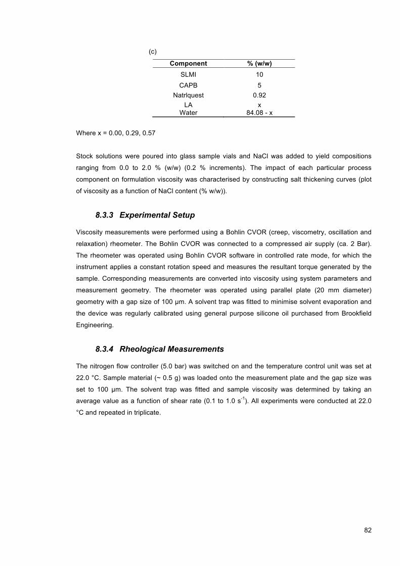
82

(c)


Natrlquest 0.92 LA x

Water 84.08 - x

Where x = 0.00, 0.29, 0.57

Stock solutions were poured into glass sample vials and NaCl was added to yield compositions

ranging from 0.0 to 2.0 % (w/w) (0.2 % increments). The impact of each particular process

component on formulation viscosity was characterised by constructing salt thickening curves (plot

of viscosity as a function of NaCl content (% w/w)).

8.3.3 Experimental Setup

Viscosity measurements were performed using a Bohlin CVOR (creep, viscometry, oscillation and

relaxation) rheometer. The Bohlin CVOR was connected to a compressed air supply (ca. 2 Bar).

The rheometer was operated using Bohlin CVOR software in controlled rate mode, for which the

instrument applies a constant rotation speed and measures the resultant torque generated by the

sample. Corresponding measurements are converted into viscosity using system parameters and

measurement geometry. The rheometer was operated using parallel plate (20 mm diameter)

geometry with a gap size of 100 µm. A solvent trap was fitted to minimise solvent evaporation and

the device was regularly calibrated using general purpose silicone oil purchased from Brookfield

Engineering.

8.3.4 Rheological Measurements

The nitrogen flow controller (5.0 bar) was switched on and the temperature control unit was set at

22.0 °C. Sample material (~ 0.5 g) was loaded onto the measurement plate and the gap size was

set to 100 µm. The solvent trap was fitted and sample viscosity was determined by taking an

average value as a function of shear rate (0.1 to 1.0 s-1). All experiments were conducted at 22.0

°C and repeated in triplicate.

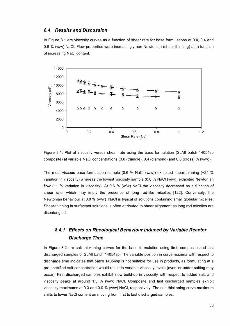
83


In Figure 8.1 are viscosity curves as a function of shear rate for base formulations at 0.0, 0.4 and

0.6 % (w/w) NaCl. Flow properties were increasingly non-Newtonian (shear thinning) as a function

of increasing NaCl content.

Figure 8.1. Plot of viscosity versus shear rate using the base formulation (SLMI batch 14054sp

composite) at variable NaCl concentrations (0.0 (triangle), 0.4 (diamond) and 0.6 (cross) % (w/w)).

The most viscous base formulation sample (0.6 % NaCl (w/w)) exhibited shear-thinning (~24 %

variation in viscosity) whereas the lowest viscosity sample (0.0 % NaCl (w/w)) exhibited Newtonian

flow (~1 % variation in viscosity). At 0.6 % (w/w) NaCl the viscosity decreased as a function of

shear rate, which may imply the presence of long rod-like micelles [122]. Conversely, the

Newtonian behaviour at 0.0 % (w/w) NaCl is typical of solutions containing small globular micelles.

Shear-thinning in surfactant solutions is often attributed to shear alignment as long rod micelles are

disentangled.

8.4.1 Effects on Rheological Behaviour Induced by Variable Reactor Discharge Time

In Figure 8.2 are salt thickening curves for the base formulation using first, composite and last

discharged samples of SLMI batch 14054sp. The variable position in curve maxima with respect to

discharge time indicates that batch 14054sp is not suitable for use in products, as formulating at a

pre-specified salt concentration would result in variable viscosity levels (over- or under-salting may

occur). First discharged samples exhibit slow build-up in viscosity with respect to added salt, and

viscosity peaks at around 1.3 % (w/w) NaCl. Composite and last discharged samples exhibit

viscosity maximums at 0.3 and 0.0 % (w/w) NaCl, respectively. The salt-thickening curve maximum

shifts to lower NaCl content on moving from first to last discharged samples.

0

2000

4000

6000

8000

10000

12000

14000

0 0.2 0.4 0.6 0.8 1 1.2

Visc

osity

(cP

)

Shear Rate (1/s)

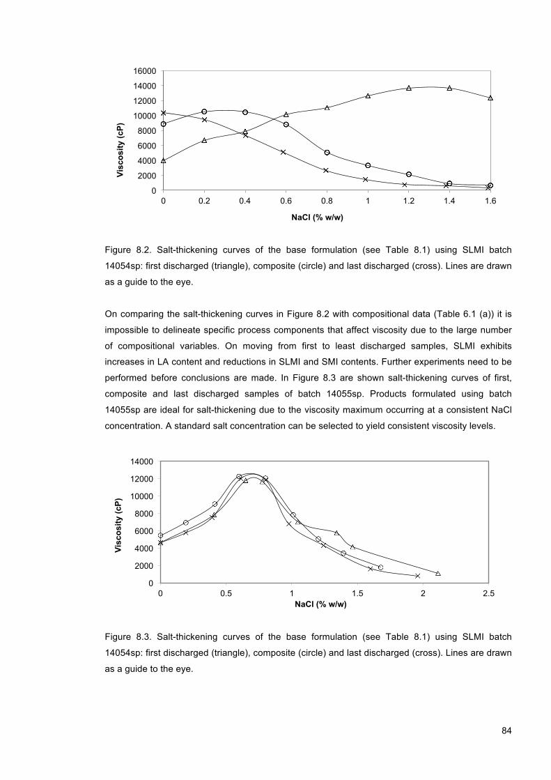
84

Figure 8.2. Salt-thickening curves of the base formulation (see Table 8.1) using SLMI batch

14054sp: first discharged (triangle), composite (circle) and last discharged (cross). Lines are drawn

as a guide to the eye.

On comparing the salt-thickening curves in Figure 8.2 with compositional data (Table 6.1 (a)) it is

impossible to delineate specific process components that affect viscosity due to the large number

of compositional variables. On moving from first to least discharged samples, SLMI exhibits

increases in LA content and reductions in SLMI and SMI contents. Further experiments need to be

performed before conclusions are made. In Figure 8.3 are shown salt-thickening curves of first,

composite and last discharged samples of batch 14055sp. Products formulated using batch

14055sp are ideal for salt-thickening due to the viscosity maximum occurring at a consistent NaCl

concentration. A standard salt concentration can be selected to yield consistent viscosity levels.

Figure 8.3. Salt-thickening curves of the base formulation (see Table 8.1) using SLMI batch

14054sp: first discharged (triangle), composite (circle) and last discharged (cross). Lines are drawn

as a guide to the eye.

0

2000

4000

6000

8000

10000

12000

14000

16000

0 0.2 0.4 0.6 0.8 1 1.2 1.4 1.6

Visc

osity

(cP)

NaCl (% w/w)

0

2000

4000

6000

8000

10000

12000

14000

0 0.5 1 1.5 2 2.5

Visc

osity

(cP)

NaCl (% w/w)

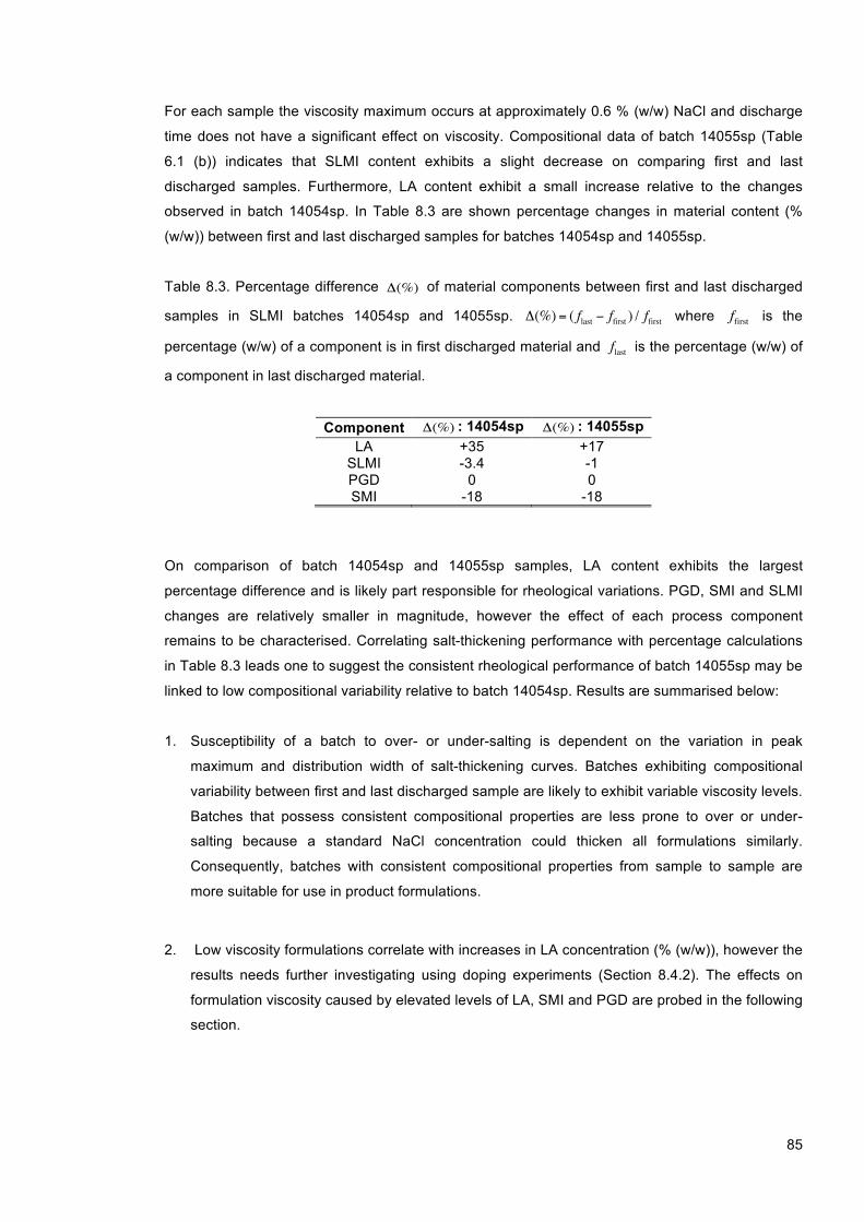
85

For each sample the viscosity maximum occurs at approximately 0.6 % (w/w) NaCl and discharge

time does not have a significant effect on viscosity. Compositional data of batch 14055sp (Table

6.1 (b)) indicates that SLMI content exhibits a slight decrease on comparing first and last

discharged samples. Furthermore, LA content exhibit a small increase relative to the changes

observed in batch 14054sp. In Table 8.3 are shown percentage changes in material content (%

(w/w)) between first and last discharged samples for batches 14054sp and 14055sp.

Table 8.3. Percentage difference Δ(%) of material components between first and last discharged

samples in SLMI batches 14054sp and 14055sp. Δ(%) = ( flast − ffirst ) / ffirst where ffirst is the

percentage (w/w) of a component is in first discharged material and flast is the percentage (w/w) of

a component in last discharged material.

Component Δ(%) : 14054sp Δ(%) : 14055sp LA +35 +17

SLMI -3.4 -1 PGD 0 0 SMI -18 -18

On comparison of batch 14054sp and 14055sp samples, LA content exhibits the largest

percentage difference and is likely part responsible for rheological variations. PGD, SMI and SLMI

changes are relatively smaller in magnitude, however the effect of each process component

remains to be characterised. Correlating salt-thickening performance with percentage calculations

in Table 8.3 leads one to suggest the consistent rheological performance of batch 14055sp may be

linked to low compositional variability relative to batch 14054sp. Results are summarised below:

1. Susceptibility of a batch to over- or under-salting is dependent on the variation in peak

maximum and distribution width of salt-thickening curves. Batches exhibiting compositional

variability between first and last discharged sample are likely to exhibit variable viscosity levels.

Batches that possess consistent compositional properties are less prone to over or under-

salting because a standard NaCl concentration could thicken all formulations similarly.

Consequently, batches with consistent compositional properties from sample to sample are

more suitable for use in product formulations.

2. Low viscosity formulations correlate with increases in LA concentration (% (w/w)), however the

results needs further investigating using doping experiments (Section 8.4.2). The effects on

formulation viscosity caused by elevated levels of LA, SMI and PGD are probed in the following

section.

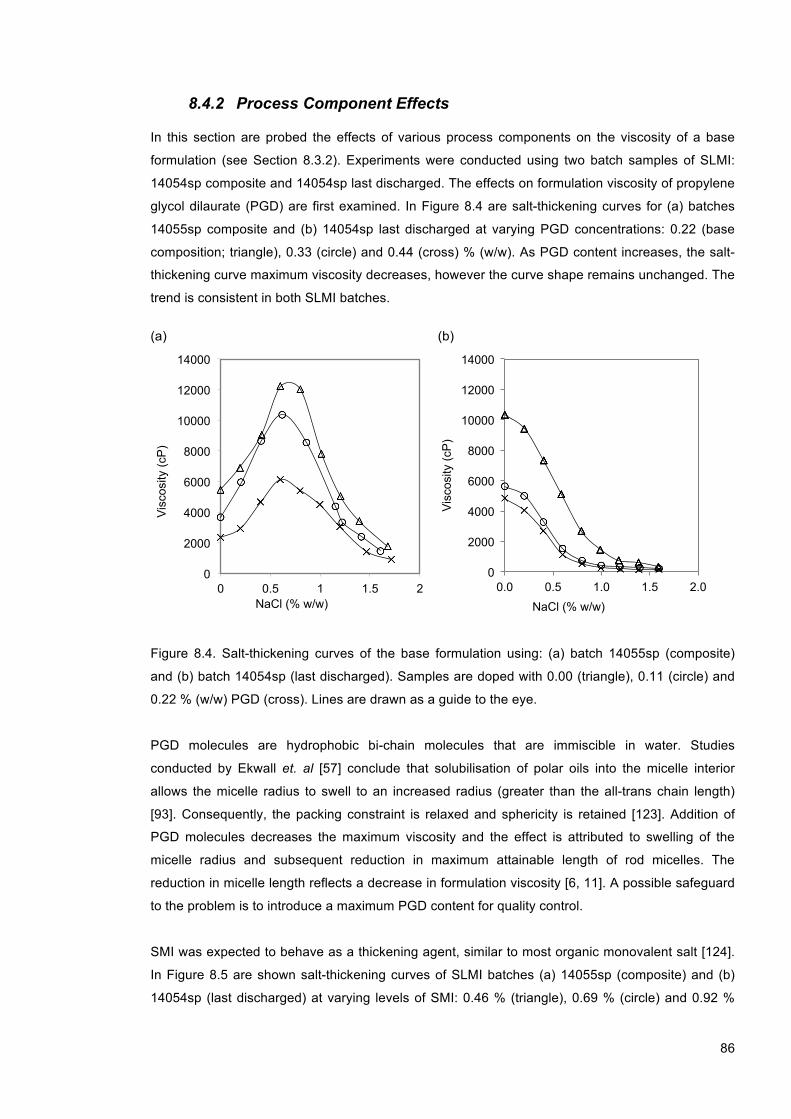
86

8.4.2 Process Component Effects

In this section are probed the effects of various process components on the viscosity of a base

formulation (see Section 8.3.2). Experiments were conducted using two batch samples of SLMI:

14054sp composite and 14054sp last discharged. The effects on formulation viscosity of propylene

glycol dilaurate (PGD) are first examined. In Figure 8.4 are salt-thickening curves for (a) batches

14055sp composite and (b) 14054sp last discharged at varying PGD concentrations: 0.22 (base

composition; triangle), 0.33 (circle) and 0.44 (cross) % (w/w). As PGD content increases, the salt-

thickening curve maximum viscosity decreases, however the curve shape remains unchanged. The

trend is consistent in both SLMI batches.

(a) (b)

Figure 8.4. Salt-thickening curves of the base formulation using: (a) batch 14055sp (composite)

and (b) batch 14054sp (last discharged). Samples are doped with 0.00 (triangle), 0.11 (circle) and

0.22 % (w/w) PGD (cross). Lines are drawn as a guide to the eye.

PGD molecules are hydrophobic bi-chain molecules that are immiscible in water. Studies

conducted by Ekwall et. al [57] conclude that solubilisation of polar oils into the micelle interior

allows the micelle radius to swell to an increased radius (greater than the all-trans chain length)

[93]. Consequently, the packing constraint is relaxed and sphericity is retained [123]. Addition of

PGD molecules decreases the maximum viscosity and the effect is attributed to swelling of the

micelle radius and subsequent reduction in maximum attainable length of rod micelles. The

reduction in micelle length reflects a decrease in formulation viscosity [6, 11]. A possible safeguard

to the problem is to introduce a maximum PGD content for quality control.

SMI was expected to behave as a thickening agent, similar to most organic monovalent salt [124].

In Figure 8.5 are shown salt-thickening curves of SLMI batches (a) 14055sp (composite) and (b)

14054sp (last discharged) at varying levels of SMI: 0.46 % (triangle), 0.69 % (circle) and 0.92 %

0

2000

4000

6000

8000

10000

12000

14000

0 0.5 1 1.5 2

Visc

osity

(cP

)

NaCl (% w/w)

0

2000

4000

6000

8000

10000

12000

14000

0.0 0.5 1.0 1.5 2.0

Visc

osity

(cP

)

NaCl (% w/w)

87

(cross) (w/w). As SMI content increased, the salt thickening curve is shifted to lower salt

concentrations and the peak viscosity value remains fairly unchanged.

(a) (b)


and (b) batch 14054sp (last discharged) at 0.00 (triangle), 0.23 (circle) and 0.46 (cross) % (w/w)

SMI. Lines are drawn as a guide to the eye.

Elevated levels of SMI reduce the effective head-group area at the micelle surface by screening

electrostatic repulsion between charged surfactant head groups [125]. As a consequence, smaller

amounts of NaCl are required to induce a sphere to rod micelle transition. Results are consistent

with a study conducted by Kumar [126] on the effects on SDS micelle morphology using a range of

electrolytes. SMI content needs be monitored to avoid over or under-salting during the formulation

process.

The final process component of study was lauric acid (LA), a C12 non-ionic carboxylic acid. Salt-

thickening curves for batches (a) 14055sp composite and (b) 14054sp last discharged doped with

LA are presented in Figure 8.6: 0.57 % LA (triangle), 0.86 % LA (circle) and 1.14 % LA (cross)

(w/w). An elevated LA content resulted in drastic reduction in formulation viscosity. The viscosity

maximum shifted to lower NaCl concentrations with increasing LA content.

0

2000

4000

6000

8000

10000

12000

14000

0 0.5 1 1.5 2

Visc

osity

(cP

)

NaCl (% w/w)

0

2000

4000

6000

8000

10000

12000

14000

0.0 0.5 1.0 1.5 2.0

Visc

osity

(cP

) NaCl (% w/w)

88

(a) (b)


and (b) batch 14054sp (last discharged), doped with 0.00 (triangle), 0.29 (circle) and 0.57 (cross)

% (w/w) LA. Lines are drawn as a guide to the eye.

LA induces significant reduction in viscosity with increasing content and must be carefully

controlled to prevent low viscosity product formulations. On comparison of salt-thickening for the

respective process components, it is evident that LA has the most significant viscosity reducing

effect.

The viscosity reducing nature of LA can be explained by considering its effects at the molecular

level. Small head-group fatty acids (such as LA) adsorb into the micelle core and reduce the

average head group area at the micelle surface [6]. The critical packing parameter increases and

micelles undergo a shape transition to a flatter aggregate structure. At increased LA levels, the

average head group area is reduced significantly and micelles predominantly exist in a disk-like

geometry, which exhibit lower viscosities. As a result, a lower NaCl concentration is required to

maximise formulation viscosity maximum. Our results are consistent with studies conducted by

Ekwall [57] on the effects on sodium octanoate phase behaviour of similar fatty acid (cosurfactant)

additives [5].

0

2000

4000

6000

8000

10000

12000

14000

0 0.5 1 1.5 2

Visc

osity

(cP

)

NaCl (% w/w)

0

2000

4000

6000

8000

10000

12000

14000

0.0 0.5 1.0 1.5 2.0

Visc

osity

(cP

)

NaCl (% w/w)

89


An elevated concentration of LA, PGD or SMI has potential to induce a reductive effect on

formulation viscosity. Elevated LA concentrations induced the most drastic reduction in formulation

viscosity and its content should be controlled and kept to a minimum. An elevated PGD

concentration also reduced solution viscosity and safeguards should be introduced to minimise its

concentration. SMI was determined to act as a thickening agent, akin to many small monovalent

salts [11]. An empirical relationship between SMI content and the optimum level of NaCl (required

for thickening in many formulation processes) is difficult to establish due to the large number of

process variables. To reduce variability in formulation viscosity, variations in process component

levels need to be minimised.

The obvious solution for limiting the extent of hydrolysis is to eliminate water release at the end of

the reaction process. In practice this is not feasible due to condensation on the upper walls of the

reactor. For the current process design, Innospec have optimised variables such as discharge rate

from the reactor and quenching efficiency of the flaker belt. The next stage of investigation is to

work towards identifying and synthesising the “ideal” SLMI composition (whilst minimising

compositional variability), which exhibits the desired rheological performance.

90

9 Micelle Build-up Kinetics in the Sodium Lauroyl Methyl Isethionate/ (Carboxylatomethyl)hexadecyldimethyl ammonium /Water System

Personal care products may contain a number of components such as surfactants, polymers,

electrolytes and fragrances. The rheological properties of a product formulation are dependent on

ingredient compatibility as well as their relative concentrations. Even if suitable components are

mixed, the formulation may be ineffective if the physicochemical properties (viscosity, pH, turbidity)

are not correctly tuned in accordance with component ratio [127].

The rheological properties of a personal care product dictate pumpability and ergonomics.

Shampoo and shower gel products often exhibit high viscosity and viscoelasticity due to the

presence of long cylindrical (rod-like) micelles in solution. On mixing individual surfactant

components micelle growth occurs and the time to attain equilibrium viscosity varies from seconds

to months. The molecular process by which equilibrium is attain is not understood [89, 128]. Slow

micelle growth kinetics may present a significant problem for formulators as the rheology may

undergo changes between leaving the factory and reaching the shop shelf. This Chapter examines

the micelle build-up kinetics in a standard formulation of SLMI, (carboxylatomethyl)

hexadecyldimethyl ammonium (cetyl betaine) and water (see Section 9.3). A ternary phase

diagram depicting liquid crystal and viscoelastic phase regions was determined as a basis for

identifying sample compositions for further study. The micelle build-up phenomenon was

characterised as a function of time after mixing using static light scattering and nuclear magnetic

resonance spectroscopy. The study objective was to obtain an improved understanding of micelle

growth kinetics.

9.1 Theoretical Descriptions of Micelle Build-up

On mixing two aqueous surfactant components above the CMC to achieve a solution composition

that exhibits viscoelastic properties, there is an increase in viscosity as a function of time. The

increase in viscosity occurs due to micelle growth from small micelles into cylindrical (rod-like)

micelles and there are two well-established theoretical descriptions [89, 129]:

(1) Monomeric addition to small micelles. The initial rate of formation of cylindrical micelles is

given by

Initial rate = k micsp!" #$ monA[ ]m monB[ ]n Equation 9.1

where n and m are experimentally determined orders of reaction with respect to surfactants A and

B. [ ]spmic , [ ]Amon and [ ]Bmon are the concentrations of small micelles, surfactant monomer A and

surfactant monomer B respectively. k is the cylindrical micelle build-up rate constant.

91

(2) Micelle Fusion. Aggregation of small micelles to form a cylindrical micelle. Initial rate of

formation of rod micelles is given by:

[ ]Pspmicrate Initial k= Equation 9.2

where P is the experimentally determined order of reaction with respect to the concentration of

small micelles. k is the cylindrical micelle build-up rate constant.

The concentration of micelles may be approximated as equal to surfactant concentration as greater

than ~98 % of surfactant molecules exist in micellar form. By determining the relationship between

k and surfactant concentration, one may distinguish between the two mechanisms. For

mechanism (1), k is expected to exhibit a linear dependence on surfactant concentration as

monomer concentrations are approximately constant (decrease slightly) above the CMC. For

mechanism (2), k is expected to increase by a power law as a function of surfactant

concentration. P may be determined experimentally from measuring the dependence of build-up

constant on surfactant concentration above the CMC.

9.2 Monitoring Micelle Growth: NMR Linewidth Broadening and Static Light Scattering

On mixing aqueous surfactant components to a solution composition exhibiting viscoelasticity,

micelle growth leads to an initial large increase in the observed linewidth obsυΔ before plateauing.

obsυΔ is a function of the number density and hydrodynamic diameter of micelles, and therefore

may be measured to monitor the micelle growth process [89, 93, 130]. For a similar C12 anionic and

C16 zwitterionic surfactant system (sodium dodecyl sulphate/hexadecyldimethylamoniopropane

sulphonate/water), Tiddy et al. found that obsυΔ was a weighted average of contributions from

surfactant molecules in small micelles SυΔ and cylindrical micelles CυΔ [89]. obsυΔ is given by

CCsSobs PP υυυ Δ+Δ=Δ Equation 9.3

where SP and CP are the fraction of surfactant molecules in small and cylindrical micelles

respectively. Previous authors have shown that CS PP >> and sC υυ >> [93]. Since 1≅SP , changes

in obsυΔ are primarily due to changes in CυΔ and Equation 9.3 may be approximated as

CCobs P υυ Δ≅Δ Equation 9.4

92

In the same study authors found that initial micelle growth kinetics were first order with respect to

the concentration of surfactant (approximately equal to concentration of small micelles). However

after an initial time period the situation was complicated by the micelle breakdown process, which

causes a fall-off in build-up rate with time. Assuming first order kinetics with respect to the

concentration of small micelles, we can derive an expression for the changes in linewidth as a

function of time. Using the first order integrated rate law we can write

))exp(1(0 ktAAcy −−= Equation 9.5

where cyA is the concentration of small micelles, 0A is the initial concentration of surfactant and k

is the micelle build-up rate constant. Since obsυΔ is a function of micelle number density and

hydrodynamic size [93], we can write

))exp(1)(( ktsphfinalobs −−Δ−Δ=Δ ννν Equation 9.6

where sphνΔ is the peak linewidth of small micelles and finalνΔ is the final peak linewidth, which

includes contributions from cylindrical and small micelles.

A similar relation can be written when following micelle build-up using static light scattering. Tiddy

et al. found that for solutions containing cylindrical micelles, the photon scattering count rate is a

function of the number density and square diameter of micelles [93]. Consequently, increases in

micelle hydrodynamic size may be monitored using this technique and micelle build-up kinetics are

also expected to follow a form of Equation 9.6.

93

9.3 Methodology

It was necessary to delineate viscoelastic and liquid crystalline phase regions in the SLMI/cetyl

betaine/H20 system at sub-10 % (w/w) surfactant concentrations. Once phase boundaries were

determined, a number of viscoelastic compositions were selected to probe micelle build-up using

NMR and SLS techniques.

Proton NMR spectra of SLMI, cetyl betaine and SLMI/cetyl betaine solutions in D2O were obtained.

An easily resolvable proton peak was identified for measuring obsυΔ to monitor micelle growth.

NMR and SLS were used to follow micelle build-up on mixing aqueous solutions of SLMI and cetyl

betaine. A range of solution compositions were studied within and outside of the viscoelastic phase

region. Experiments were conducted:

a) As a function of total surfactant concentration (% (w/w)) at fixed SLMI:cetyl betaine ratio

(w:w).

b) As a function of SLMI:cetyl betaine ratio (w:w) at fixed total surfactant concentration (%

(w/w)).

Experiment a) was conducted to study the dependence of micelle build-up rate constant on

surfactant concentration and distinguish between the monomer addition and fusion growth

mechanisms. The micelle build-up rate constant for monomer addition to small micelles was

expected to vary linearly with surfactant concentration. Conversely, the build-up rate constant for

micelle fusion was expected to increase rapidly as a function of surfactant concentration (see

Section 9.1 and 9.2). Experiment b) was conducted to determine the dependence of micelle build-

up constant on surfactant mass ratio.


9.4.1 Phase Diagram Determination

All glassware was washed with nitric acid (0.5 M) and Mili-Q water. Stock solutions of SLMI (batch

14055sp composite)/water and cetyl betaine/water (10.0 % (w/w)) were prepared and diluted with

Mili-Q water to yield solution concentrations ranging from 0.1 to 5.0 % (w/w). The viscoelastic

boundary was determined by titrating SLMI solutions to cetyl betaine solutions (and vice-versa;

order of addition achieved same result) in a stirred beaker. Viscoelastic solutions were identified by

recoil on swirling and shear birefringence when viewed between crossed polarisers). The SLMI-rich

side of the viscoelastic boundary was relatively difficult to determine due to slow kinetics. Liquid

crystal phase boundaries were determined by preparing mixed surfactant samples over narrow

concentration intervals. Mixed samples were left to equilibrate for one week and were visually

94

observed for formation (single phase) or separation (biphasic) of liquid crystalline phase. A ternary

phase diagram was plotted using OriginPro (v9.1) software.

9.4.2 NMR Spectroscopy

NMR tubes (8 mm diameter, Sigma) and relevant glassware were washed with nitric acid (0.5 M)

and Mili-Q water. Master solutions (20.0 % (w/w)) of SLMI (batch 14055sp composite)/water and

cetyl betaine/water were prepared and diluted with D2O to yield concentrations ranging from 0.1 to

5.0 % (w/w), The diluted samples were filtered through 0.45 µm Millex-HV filters purchased from

Millipore Corp. Samples were equilibrated at 20.0 °C for one week prior to measurement.

SLMI/cetyl betaine/D2O samples were prepared by mixing aqueous surfactant components in a

glass vial. The solution was immediately transferred to an NMR tube and placed in the

spectrometer. The experimental delay time was ~3 minutes due to sample shimming. 1H NMR

spectra were recorded as a function of time until constant linewidths were attained (~12 scans per

data point). The time dependence of SLMI β-CH2 proton peak linewidth was used to monitor

micelle build-up. Samples were monitored as a function of surfactant concentration (2.0 to 4.0 %

(w/w); SLMI:cetyl betaine ratio 1:2 (w:w)) and as a function of mass ratio (SLMI:cetyl betaine 1:1 to

1:3 (w:w). 2.0 % (w/w)). Experiments were repeated using batch 14055sp composite.


Proton NMR experiments were conducted using a Bruker Avance III 800 MHz NMR Spectrometer

(0.54 T magnetic field) with a 1H/13C/15N TCI cryoprobe. The dead time of the spectrometer is

accounted for by d1 (radiofrequency oscillator probe) and d2 (receiver). d1 is the time between

applying the radiofrequency pulse and data collection. d2 is the wait time for the filter to stabilise.

The pulse sequence (zgesgp) represented a standard proton one-dimensional experiment with

excitation sculpting water suppression and is described as follows [131]:

d1 (relaxation delay); 1H 90°; gradient 1; shaped 1H 180° (selective on water); 1H 180° (-x);

gradient 1 (refocuses 1H except water); gradient 2; shaped 1H 180° (selective on water); 1H 180° (-

x); gradient 2 (refocuses 1H except water); acquire.

The spectrometer was fitted with a temperature control unit accurate to ± 0.05 °C. Samples were

loaded into NMR tubes (8mm diameter, glass) and inserted into the sample holder. The numbers of

scans were manually adjusted depending on the type of experiment and ranged from 16 to 512.

Linewidths were measured at half height using Topspin (v3.2) software.

95

9.4.3 Static Light Scattering

A low volume quartz cuvette (45 µL) and relevant glassware were washed with nitric acid (0.5 M)

and Mili-Q water. Master solutions of SLMI (20.0 % (w/w)) and cetyl betaine (20.0 % (w/w)) were

prepared and diluted with H2O to yield concentrations ranging from 0.1 to 5.0 % (w/w), The diluted

samples were filtered through 0.45 µm Millex-HV filters purchased from Millipore Corp. Samples

were equilibrated at 20.0 °C for one week prior to measurement. Experiments were conducted as a

function of surfactant concentration (2.0 to 4.0 % (w/w). SLMI:cetyl betaine 1:2 (w:w)) and as a

function of mass ratio (2.0 % (w/w). SLMI:cetyl betaine 1:1 to 1:3 (w:w)). SLMI/cetyl betaine/H2O

solutions were prepared by mixing aqueous surfactant components the cuvette. Photon count rate

was measured at a 90° detection angle as a function of time after mixing for a range of samples

inside and outside of the viscoelastic region. Each data point comprised an average from 11 scans.

Experiments were repeated using batch 14055sp composite.


The photon count rate (scattering intensity) of SLMI micelles in electrolyte solution were measured

using a Malvern Zetasizer Nano-S instrument operating a He–Ne laser (632.8 nm). The actuator

setting was automatic and data was collected at a scattering angle of 90.0°. All experiments were

performed at 20.0 °C and the error in temperature measurement was ± 0.05 °C. Samples were

placed in a low volume quartz cuvette (45 µL). Malvern Dispersion Technology Software (DTS)

v5.03 was used for data analysis.

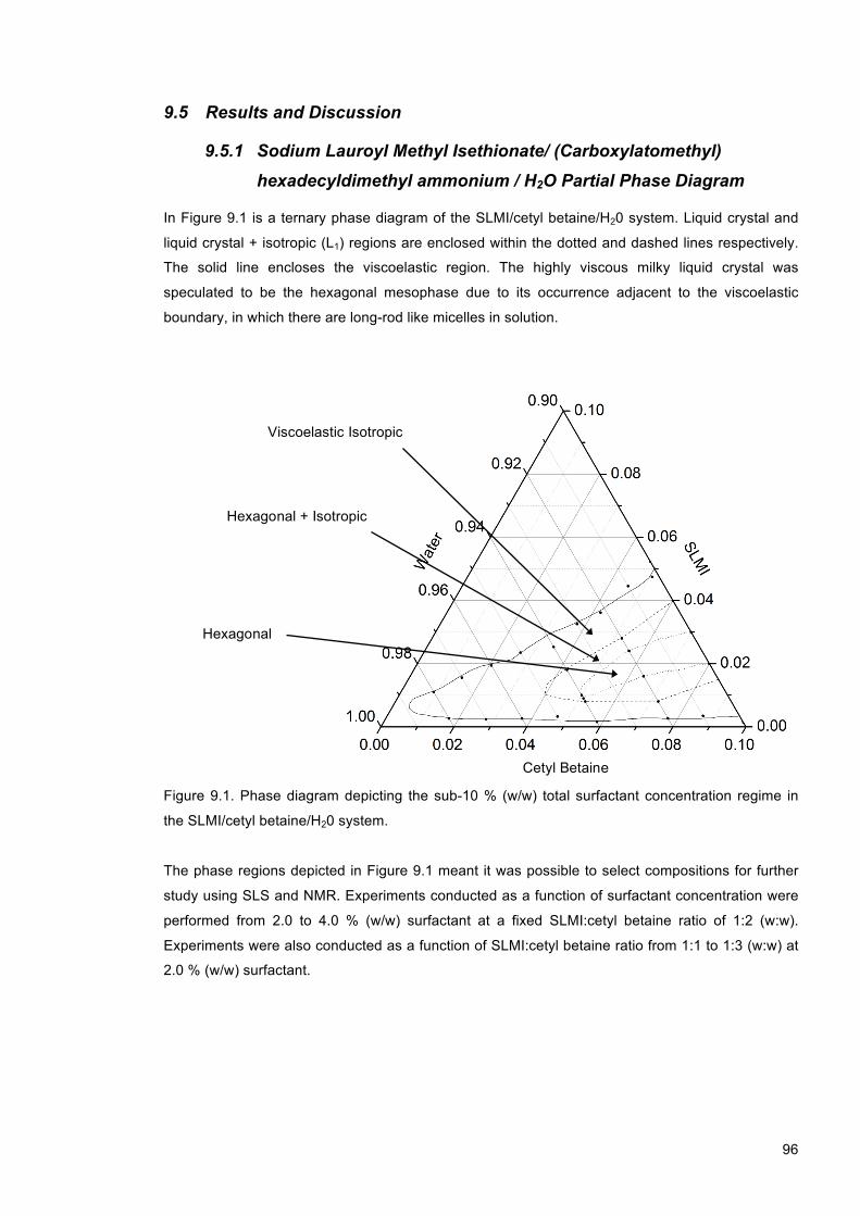
96


9.5.1 Sodium Lauroyl Methyl Isethionate/ (Carboxylatomethyl) hexadecyldimethyl ammonium / H2O Partial Phase Diagram

In Figure 9.1 is a ternary phase diagram of the SLMI/cetyl betaine/H20 system. Liquid crystal and

liquid crystal + isotropic (L1) regions are enclosed within the dotted and dashed lines respectively.

The solid line encloses the viscoelastic region. The highly viscous milky liquid crystal was

speculated to be the hexagonal mesophase due to its occurrence adjacent to the viscoelastic

boundary, in which there are long-rod like micelles in solution.

Figure 9.1. Phase diagram depicting the sub-10 % (w/w) total surfactant concentration regime in

the SLMI/cetyl betaine/H20 system.

The phase regions depicted in Figure 9.1 meant it was possible to select compositions for further

study using SLS and NMR. Experiments conducted as a function of surfactant concentration were

performed from 2.0 to 4.0 % (w/w) surfactant at a fixed SLMI:cetyl betaine ratio of 1:2 (w:w).

Experiments were also conducted as a function of SLMI:cetyl betaine ratio from 1:1 to 1:3 (w:w) at

2.0 % (w/w) surfactant.

Viscoelastic Isotropic

Hexagonal

Hexagonal + Isotropic

Cetyl Betaine

97

9.5.2 Solution State Proton NMR of Surfactant Components

In Figure 9.2 is the 1H NMR spectrum of SLMI in D20 (5.0 % (w/w)). Peak assignments are listed in

Table 9.1. Discrepancies in the integrated peak intensity (H’s (Int.)) are due to the presence of

additional process components within SLMI (see Table 6.1).

Table 9.1. 1H NMR peak assignments of SLMI in D20 (5.0 % (w/w)). H’s (Int.) is the integrated peak

intensity and was calculated using Topspin software. H’s is the actual number of protons.

Shift (ppm) Intensity H’s (Int.) H’s Assignment 0.802 1 3.00 3 CH3(CH2)10 1.23 7.34 22.02 20 (CH2)8; COOC(CH3); COOCH

1.546 0.721 2.16 2 CH3(CH2)8CH2 2.27 0.642 1.93 2 CH3(CH2)8CH2CH2 3.01 0.327 0.98 1 CH2βSO3Na

3.131 0.305 0.92 1 CH2αSO3Na

ΣH = 31 29

In Figure 9.3 is the 1H NMR spectrum of the cetyl betaine/D20 system (5.0 % (w/w)). The peaks

assignments are listed in Table 9.2. Discrepancies in peak intensity are due to the presence of

additional process components within cetyl betaine (see Table 6.4).

Table 9.2. 1H NMR peak assignments of cetyl betaine in D20 (5.0 % (w/w)).

Shift (ppm) Intensity H’s (Int.) H’s Assignment 0.804 1 3.00 3 CH3(CH2)15 1.224 7 21.00 26 CH3(CH2)13 1.652 0.691 2.07 2 CH3(CH2)13CH2 3.14 1.96 5.88 6 N(CH3)2

3.527 0.353 1.06 2 CH3(CH2)13CH2CH2 3.762 0.352 1.06 3 CH2COO

ΣH = 34 32

In Figure 9.4 is the 1H NMR spectrum of a SLMI/cetyl betaine/D20 sample (5.0 % (w/w). SLMI:cetyl

betaine ratio 1:2 (w:w)). The SLMI (CH2)8CH2CH2 (β-CH2) proton signal was easily resolved and

was selected for characterising micelle build up. The SLMI β-CH2 linewidth was taken as the

linewidth at half peak height, and was calculated using Topspin software (see Section 9.4.2).

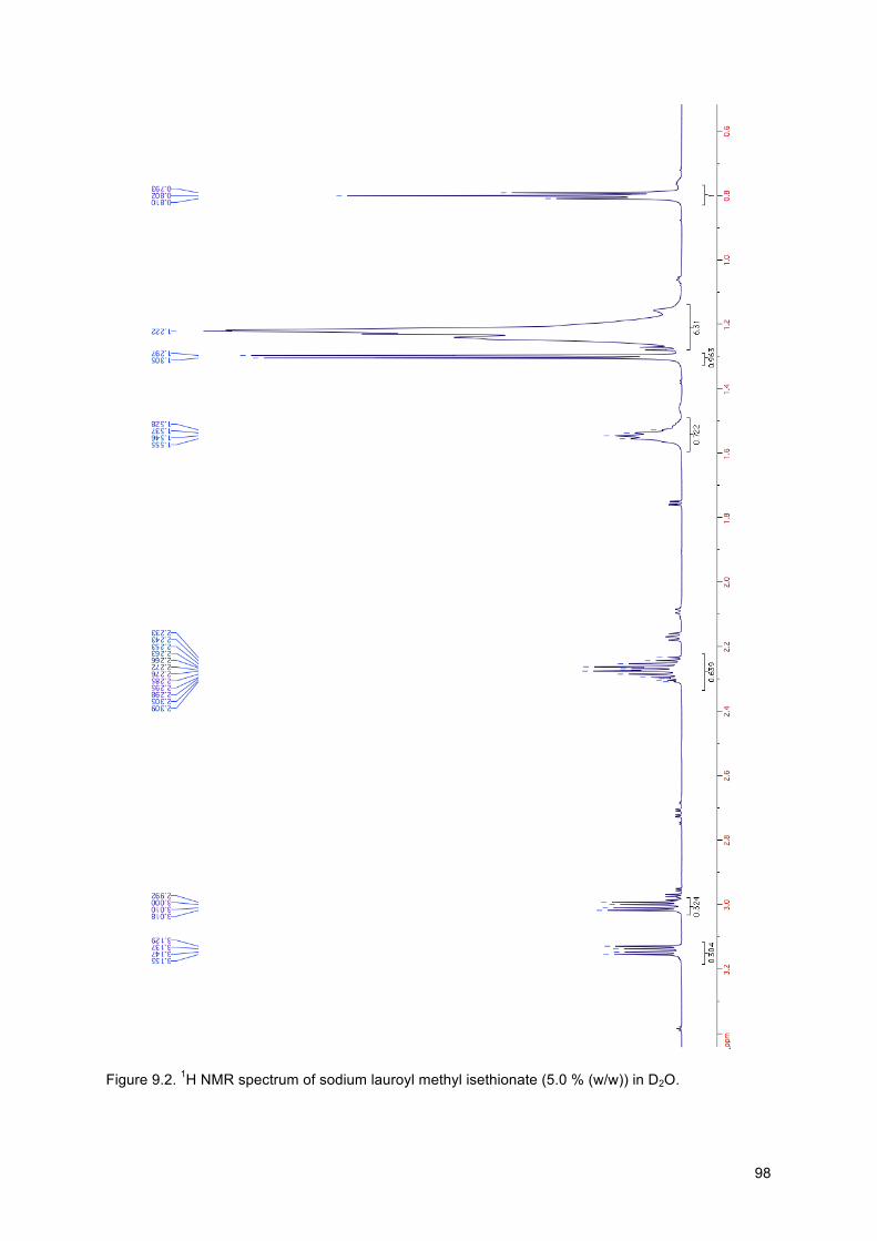
98

Figure 9.2. 1H NMR spectrum of sodium lauroyl methyl isethionate (5.0 % (w/w)) in D2O.

99

Figure 9.3. 1H NMR spectrum of cetyl betaine (5.0 % (w/w)) in D2O.

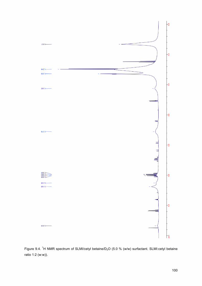
100

Figure 9.4. 1H NMR spectrum of SLMI/cetyl betaine/D2O (5.0 % (w/w) surfactant. SLMI:cetyl betaine

ratio 1:2 (w:w)).

101

9.5.3 Micelle Build-up Kinetics as a Function of Surfactant Concentration

In Figure 9.5 are plotted a) photon scattering count rate and b) 1H NMR linewidth of SLMI β-CH2

protons as a function of time for SLMI/cetyl betaine/water (2.0 to 5.0 % (w/w). SLMI:cetyl betaine

ratio 1:2 (w:w)) mixtures. The photon count rate and NMR linewidth exhibited an increase as a

function of time due to micelle growth. The rate of formation of large micelles increased as a

function of surfactant concentration, as indicated by the reduced time taken to reach an

approximately constant photon count rate/NMR linewidth.

(a) (b)

Figure 9.5. (a) Photon count rate and (b) NMR linewidth as a function of time for 2.0 (cross), 3.0

(triangle), 4.0 (circle) and 5.0 (diamond) % (w/w) SLMI/cetyl betaine/water mixtures (SLMI:cetyl

betaine ratio 1:2 (w:w)). Equation 9.7 is fitted to both sets of data, as indicated by the black lines.

It is theoretically possible to distinguish between the micelle growth mechanisms of monomeric

addition to small micelles and micelle fusion by determining the relationship between micelle build-

up rate constant and surfactant concentration (see Section 9.2). NMR linewidth and SLS count rate

were expected to follow Equation 9.6, which is re-written as

))exp(1)(()( ktxxtx spcy −−−= Equation 9.7

where k is the micelle build-up constant, x(t) the photon count rate or NMR linewidth at time t after

mixing. cyx and spx are initial and final photon count rates or NMR linewidths respectively. Micelle

build-up rate constants k were calculated by fitting the photon count rate and NMR linewidth data

0

2000

4000

6000

8000

10000

12000

14000

16000

18000

20000

1 21 41

Cou

nt R

ate

(kcp

s)

Time (mins)

0

10

20

30

40

50

60

70

80

90

100

3 23 43 63

Line

wid

th (H

z)

Time (mins)

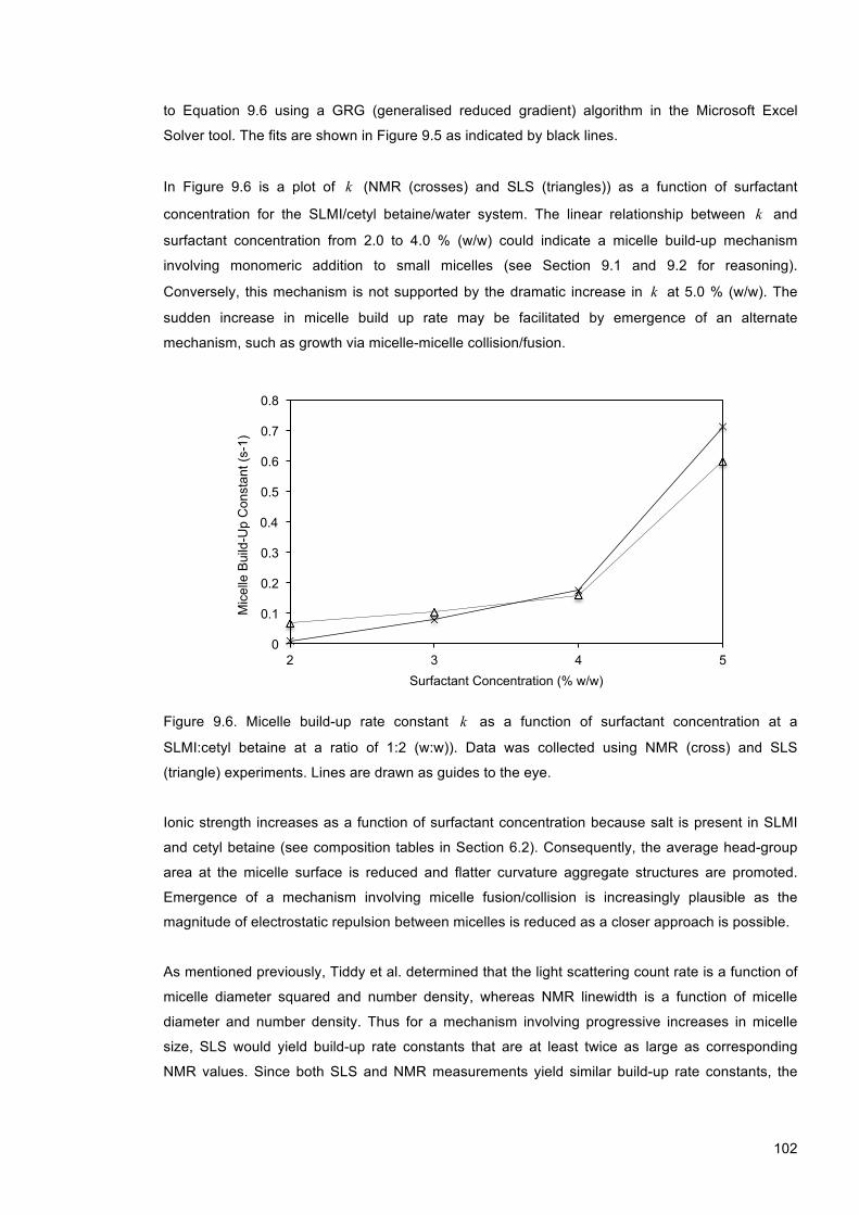
102

to Equation 9.6 using a GRG (generalised reduced gradient) algorithm in the Microsoft Excel

Solver tool. The fits are shown in Figure 9.5 as indicated by black lines.

In Figure 9.6 is a plot of k (NMR (crosses) and SLS (triangles)) as a function of surfactant

concentration for the SLMI/cetyl betaine/water system. The linear relationship between k and

surfactant concentration from 2.0 to 4.0 % (w/w) could indicate a micelle build-up mechanism

involving monomeric addition to small micelles (see Section 9.1 and 9.2 for reasoning).

Conversely, this mechanism is not supported by the dramatic increase in k at 5.0 % (w/w). The

sudden increase in micelle build up rate may be facilitated by emergence of an alternate

mechanism, such as growth via micelle-micelle collision/fusion.

Figure 9.6. Micelle build-up rate constant k as a function of surfactant concentration at a

SLMI:cetyl betaine at a ratio of 1:2 (w:w)). Data was collected using NMR (cross) and SLS

(triangle) experiments. Lines are drawn as guides to the eye.

Ionic strength increases as a function of surfactant concentration because salt is present in SLMI

and cetyl betaine (see composition tables in Section 6.2). Consequently, the average head-group

area at the micelle surface is reduced and flatter curvature aggregate structures are promoted.

Emergence of a mechanism involving micelle fusion/collision is increasingly plausible as the

magnitude of electrostatic repulsion between micelles is reduced as a closer approach is possible.

As mentioned previously, Tiddy et al. determined that the light scattering count rate is a function of

micelle diameter squared and number density, whereas NMR linewidth is a function of micelle

diameter and number density. Thus for a mechanism involving progressive increases in micelle

size, SLS would yield build-up rate constants that are at least twice as large as corresponding

NMR values. Since both SLS and NMR measurements yield similar build-up rate constants, the

0

0.1

0.2

0.3

0.4

0.5

0.6

0.7

0.8

2 3 4 5

Mic

elle

Bui

ld-U

p C

onst

ant (

s-1)

Surfactant Concentration (% w/w)

103

observed kinetics are most likely due to an increase in number density of large micelles, as

opposed to increases in the maximum micelle size.

9.5.4 Micelle Build-up Kinetics as a Function of SLMI:Cetyl Betaine Mass Ratio

1H NMR and SLS experiments were conducted to measure the dependence of micelle build-up rate

on SLMI:cetyl betaine mass ratio. Experiments were conducted for a range of SLMI:cetyl betaine

ratios (w:w) for 2.0 % (w/w) compositions. By combining all sets of data it was possible to obtain

further information on the micelle build-up process and identify procedures for avoiding slow

kinetics. In Figure 9.7 are plotted a) photon count rate and b) 1H NMR linewidth of SLMI β-CH2

protons as a function of time for SLMI/cetyl betaine/water mixtures (2.0 % (w/w)) at surfactant

ratios ranging from 1:1 to 1:3 (w:w). In both sets of data, the rate of micelle growth increases as a

function of increasing cetyl betaine mass fraction, as indicated by a decrease in time taken for the

experimental variable (count rate or linewidth) to attain an approximately constant value. Equation

9.7 is fitted to the data and is indicated by black lines.

(a) (b)

Figure 9.7. (a) Photon count rate and (b) NMR linewidth of SLMI β-CH2 resonance signal as a

function of time for SLMI/cetyl betaine/water mixtures at a fixed total surfactant concentration of 2.0

% (w/w) for SLMI:cetyl betaine ratios of 1:1 (cross), 2:3 (triangle), 1:2 (circle) and 1:3 (plus) (w:w).

Equation 9.7 is fitted to the data and is indicated by black lines.

The origin of fast kinetics in cetyl betaine rich solutions is understood in terms of DLVO theory by

considering a hypothetical scenario of two micelles each comprising ten SLMI or cetyl betaine

molecules. The first micelle is cetyl betaine rich and the second SLMI rich. The SLMI rich micelle

0

2000

4000

6000

8000

10000

12000

14000

16000

18000

20000

0 20 40 60 80

Cou

nt R

ate

(kcp

s)

Time (mins)

0

10

20

30

40

50

60

70

80

90

0 20 40 60 80

Line

wid

th (H

z)

Time (mins)

104

possesses more anionic surface charge relative to the cetyl betaine rich micelle. Consequently, the

SLMI rich micelles exhibit a greater electrostatic surface repulsion, which poses a barrier to

monomer addition or fusion and slows kinetics. In addition, cetyl betaine rich solutions form large

cylindrical micelles contrary to SLMI rich solutions, which form smaller globular micelles.

Subsequently, for cetyl betaine rich solutions containing large rod-like micelles there is an increase

in magnitude of van der Waals and depletion forces, which could lead to an increase in fusion rate.

The mixed CMC of an anionic/zwitterionic aqueous mixture is significantly lower than the average

CMC of individual surfactant components due to non-ideal electrostatic interactions between the

different head groups. Studies on an aqueous C12 anionic/C12 (and C14) zwitterionic system by

Iwasaki et al. report a minimum CMC and maximum micelle size at a surfactant mole fraction of 0.6

(zwitterionic/anionic), independent of zwitterionic chain length [132].

In Figure 9.8 is a plot of micelle build-up rate constant k as a function of SLMI:cetyl betaine mass

ratio (2.0 % w/w). Both photon count rate (cross) and linewidth (triangle) data indicate that the

micelle build up rate increases as a function of the relative proportion of cetyl betaine.

Figure 9.8. Micelle build up rate constant k for SLMI/cetyl betaine/water mixtures (2.0 % (w/w)) as

a function of SLMI:cetyl betaine mass ratio. NMR (cross) and LS (triangle) data are plotted.

The discrepancy in k at SLMI:cetyl betaine mass ratios of 1:2 and 1:3 is most likely attributed to

the dependence of each experimental parameter (count rate and linewidth) on particle size. The

intensity of scattered light from micelles is a function of the number density and square of the

hydrodynamic size of micelles. Conversely, NMR linewidth is a function of number density and the

hydrodynamic size of micelles and is therefore expected to exhibit a build-up rate that is at least a

factor of two smaller than for SLS. The larger value in micelle build up constant for SLS relative to

NMR experiments at SLMI:cetyl betaine mass ratios of 1:2 and 1:3 imply that the micelle growth

0

0.1

0.2

0.3

0.4

0.5

0.6

0.7

0.8

1:1 2:3 1:2 1:3

Bui

ld-U

p C

onst

ant k

s-1

Mass Ratio (SLMI:CB)

105

mechanism could involve an increase in maximum micelles size. Such a result is not in agreement

with analogous experiments conducted as a function of surfactant concentration.

From determining k as a function of surfactant mass ratio it is apparent that the micelle build-up

kinetics are faster as the cetyl betaine surfactant mass fraction increases. For industrial formulators

this is useful information as slow kinetics are undesirable when constructing products in house.

Formulating anionic/zwitterionic betaine aqueous mixtures at a greater surfactant mass fraction of

cetyl betaine will likely reduce equilibration time.


Our results indicate that the micelle build-up process is not explicable in terms of either monomeric

addition to small micelles or micelle fusion. At low surfactant concentrations, the linear dependence

of micelle build-up rate constant on surfactant concentration may indicate micelle growth via

monomeric addition to micelles. However as surfactant concentration is increased, faster kinetics

are observed and a fusion mechanism may provide the most likely explanation.

Micelle build-up rate constants derived via SLS and NMR as a function of concentration yielded

comparable values. The outcome implies that micelle growth does not occur via increases in the

maximum hydrodynamic size of the micelles, but rather there is an increase in cylindrical micelle

number density. Conversely, analogous experiments performed as a function of SLMI:cetyl betaine

mass ratio at fixed surfactant concentration yielded larger micelle build-up rate constants

determined by SLS relative to those by NMR for higher cetyl betaine surfactant mass fraction

compositions. At the current stage it is not clear whether micelle growth occurs as an increase in

the maximum micelle size, and more data needs to be collected before conclusions are made.

This is an initial study and there are several areas to explore before non-equilibrium micelle

kinetics can be understood. First of all, it is necessary to determine micelle breakdown rate

constants on dilution of viscoelastic mixtures so that equilibrium constants may be calculated.

Secondly, it may be worthwhile to conduct analogous experiments using high purity surfactants

that possess the same carbon chain length. Use of high purity surfactants will eliminate additional

interactions induced by unwanted process components.

106

10 Electrolyte Induced Precipitation in the Sodium Lauroyl Methyl Isethionate/Water System

Electrolytes are used as thickening agents in a variety of consumer products such as shampoos,

conditioners and shower gels. To achieve the desired rheological properties, it is important to

understand how electrolytes interact with other components in solution. In ionic surfactant systems,

demixing occurs at the cloud point, which is induced by increasing salt concentration above a

threshold value. The mechanistic detail of the electrolyte-induced cloud point is unknown and we

aim to develop an improved understanding of ion-micelle interactions. In this chapter, dynamic and

static light scattering experiments are conducted on the SLMI/”electrolyte”/water system to

investigate the cloud point phenomenon. Various salt types were tested to probe ion specificity and

Hofmeister effects [51].

10.1 Clouding in Surfactant Systems

The cloud point has been extensively documented in aqueous non-ionic (polyoxyethylene)

surfactant systems and is commonly achieved by increasing the system temperature above a

critical value. In the temperature-concentration phase diagram of a surfactant, the lower consolute

curve signifies a boundary of stability, above which the system demixes into two phases: one

surfactant-rich phase and the other surfactant-depleted. Clouding in aqueous non-ionic surfactant

systems is ascribed to the gradual dehydration of hydrophilic groups in the micelle at increased

temperatures. The cloud point phenomenon occurs as a consequence of an attractive inter-micellar

potential, the well depth of which increases as a function of temperature [133]. At solution

conditions corresponding to the cloud point, micelles possess sufficient attraction to cluster

together. The onset of clouding is indicated by a sudden increase in turbidity and subsequent

demixing [134].

After almost a century of research, significant theoretical developments have been made and the

non-ionic cloud point mechanism is for the most part understood [49, 92, 134]. In early attempts,

Kjellander et al. [135] used Flory-Huggins theory to describe cloud point behaviour and deemed the

existence of rod micelles at the cloud point a requirement to account for experimentally observed

critical volume fractions [136]. More recently, nuclear magnetic resonance spectroscopy, light

scattering and neutron scattering experiments have provided strong evidence to support an

alternate theory that micelles remain small and cluster together at temperatures approaching the

cloud point [92, 137, 138]. It is now established that polyoxyethylene surfactants with large

oxyethylene groups exhibit association between small micelles at increased temperatures.

Conversely, polyoxyethylene surfactants with small oxyethylene groups undergo a rod to disc

micelle transition at cloud point temperatures [139].

107

Cloud point behaviour is less frequently reported for ionic surfactant systems. The general absence

of a cloud point is attributed to inter-micellar electrostatic repulsion between charged surfactant

head-groups, which may provide a significant barrier to aggregation. The addition of particular

additives (secondary surfactants (non-ionic, counter charged or zwitterionic), cosurfactants and

electrolytes) to aqueous ionic surfactant mixtures have been found to induce cloud point behaviour

[125, 140, 141].

10.2 Introduction to Colloidal Interactions

The net interaction between colloidal particles in aqueous solution is often described using

Derjaguin, Landau, Verwey and Overbeek (DLVO) theory, which encompasses an attractive van

der Waals force and a repulsive electrostatic double-layer force [10].

The van der Waals (vdW) force term includes contributions from quantum mechanical dispersion

interactions (London Force), thermally averaged dipole-dipole interactions (Keesom force) and

dipole-induced dipole (Debye force) interactions. The simplest way to calculate the vdW force

between particles is to assume pairwise additivity and discount many-body interactions using the

Hamaker approach, which is sufficient for most experimental scenarios [58]. A more rigorous

description of vdW forces is presented in Lifshitz theory, which accounts many-body particle

interactions [142]. The vdW force between micelles in aqueous electrolyte solution is dependent on

the size and curvature of aggregates. Large flat structures such as disc micelles experience a

greater vdW attraction than smaller high curvature structures such as small micelles. For a given

surfactant volume fraction, disk-disk attraction is greater than rod-rod attraction, which is greater

than sphere-sphere attraction [143].

Charged micelles are surrounded by an electrical double-layer at the micelle surface, which

comprises a build-up in counter-ion charge density that screens electrostatic potential originating

from surface charge. The width of the double layer is determined by competition between counter-

ion thermal motion and electrostatic effects, which attract counter-ions towards the surface and

repel co-ions. In DLVO theory the force between two double layers is always repulsive according to

Poisson-Boltzmann mean-field theory. At high salt concentration the Poisson-Boltzmann approach

is inaccurate due to a few important oversimplifications [144]. Firstly, ions are treated as point

charges and finite-size elements are neglected. An additional oversimplification is use of a single

dielectric constant to describe the whole system. In anionic micellar solutions the charged micelle

surface and bulk solvent exhibit differing dielectric constants. The inside of the micelle is at a low

dielectric (~2) relative to water at the micellar surface (~80) [145-151].

108

10.3 Methodology

The purpose of this work was to obtain molecular level information of the electrolyte-induced cloud

point by probing electrolyte-micelle interactions. A range of salts were selected for testing from the

Hofmeister series, which ranks ions based on salting-out potency (Section 4.1). Anion specific

interactions with surfactant micelles were probed using a range of sodium salts (sodium is a

“neutral” salting-out Hofmeister cation [52]): NaCl, Na2HPO4, NaNO3, NaSCN). Cation specific

interactions with surfactant micelles were probed using a variety of chloride salts (chloride is a

“neutral” salting-out Hofmeister anion): NaCl, NH4Cl, LiCl, KCl). Cloud point curves were

determined via turbidity measurements (Section 10.3.1).

Dynamic and static light scattering techniques were utilised to characterise SLMI micelles at salt

concentrations prior to the cloud point. DLS was used to determine the hydrodynamic diameter and

polydispersity of surfactant micelles as a function of electrolyte concentration. SLS was used to

measure the photon count rate as a function of electrolyte concentration. DLS and SLS data

provided information on microstructural changes and enable qualitative estimates of micelle shape

at the cloud point.

Note: concentration units are expressed in moles per kilogram of solution (mol/kg molality) unless

specified otherwise.


10.4.1 Cloud Point Determination

Glassware was washed using nitric acid (1.0 M) and Mili-Q water. A SLMI (batch 14055sp

composite)/water stock solution (2.0 mol/kg, 50.0 ml) was prepared and diluted using Mili-Q water.

Cloud points were visually determined via turbidity measurements using a PC 950 Brinkmann

Probe Colorimeter. SLMI/water solutions were magnetically stirred and titrated with concentrated

electrolyte solution. Changes in turbidity were measured as a function of salt solution mass. The

mass of salt required to induce cloudiness (turbidity intensity < 10 (scale from 0 to 100 %

transmittance)) denoted the cloud point. Data were collected across a range of surfactant

concentrations (1 µmol/kg to 1 mol/kg). All measurements were performed at 20.0 °C and were

repeated in triplicate using NaCl, Na2HPO4, NaNO3, NaSCN, NH4Cl, LiCl and KCl

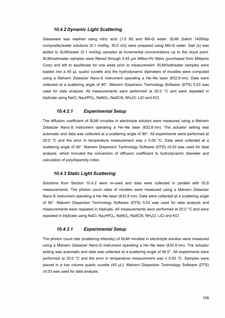
109

10.4.2 Dynamic Light Scattering

Glassware was washed using nitric acid (1.0 M) and Mili-Q water. SLMI (batch 14055sp

composite)/water solutions (0.1 mol/kg, 30.0 ml)) were prepared using Mili-Q water. Salt (s) was

added to SLMI/water (0.1 mol/kg) samples at incremental concentrations up to the cloud point.

SLMI/salt/water samples were filtered through 0.45 µm Millex-HV filters (purchased from Millipore

Corp) and left to equilibrate for one week prior to measurement. SLMI/salt/water samples were

loaded into a 45 µL quartz cuvette and the hydrodynamic diameters of micelles were computed

using a Malvern Zetasizer Nano-S instrument operating a He–Ne laser (632.8 nm). Data were

collected at a scattering angle of 90°. Malvern Dispersion Technology Software (DTS) 5.03 was

used for data analysis. All measurements were performed at 20.0 °C and were repeated in

triplicate using NaCl, Na2HPO4, NaNO3, NaSCN, NH4Cl, LiCl and KCl.


The diffusion coefficient of SLMI micelles in electrolyte solution were measured using a Malvern

Zetasizer Nano-S instrument operating a He–Ne laser (632.8 nm). The actuator setting was

automatic and data was collected at a scattering angle of 90°. All experiments were performed at

20.0 °C and the error in temperature measurement was ± 0.05 °C. Data were collected at a

scattering angle of 90°. Malvern Dispersion Technology Software (DTS) v5.03 was used for data

analysis, which included the conversion of diffusion coefficient to hydrodynamic diameter and

calculation of polydispersity index.

10.4.3 Static Light Scattering

Solutions from Section 10.4.2 were re-used and data were collected in parallel with DLS

measurements. The photon count rates of micelles were measured using a Malvern Zetasizer

Nano-S instrument operating a He–Ne laser (632.8 nm). Data were collected at a scattering angle

of 90°. Malvern Dispersion Technology Software (DTS) 5.03 was used for data analysis and

measurements were repeated in triplicate. All measurements were performed at 20.0 °C and were

repeated in triplicate using NaCl, Na2HPO4, NaNO3, NaSCN, NH4Cl, LiCl and KCl


The photon count rate (scattering intensity) of SLMI micelles in electrolyte solution were measured

using a Malvern Zetasizer Nano-S instrument operating a He–Ne laser (632.8 nm). The actuator

setting was automatic and data was collected at a scattering angle of 90.0°. All experiments were

performed at 20.0 °C and the error in temperature measurement was ± 0.05 °C. Samples were

placed in a low volume quartz cuvette (45 µL). Malvern Dispersion Technology Software (DTS)

v5.03 was used for data analysis.

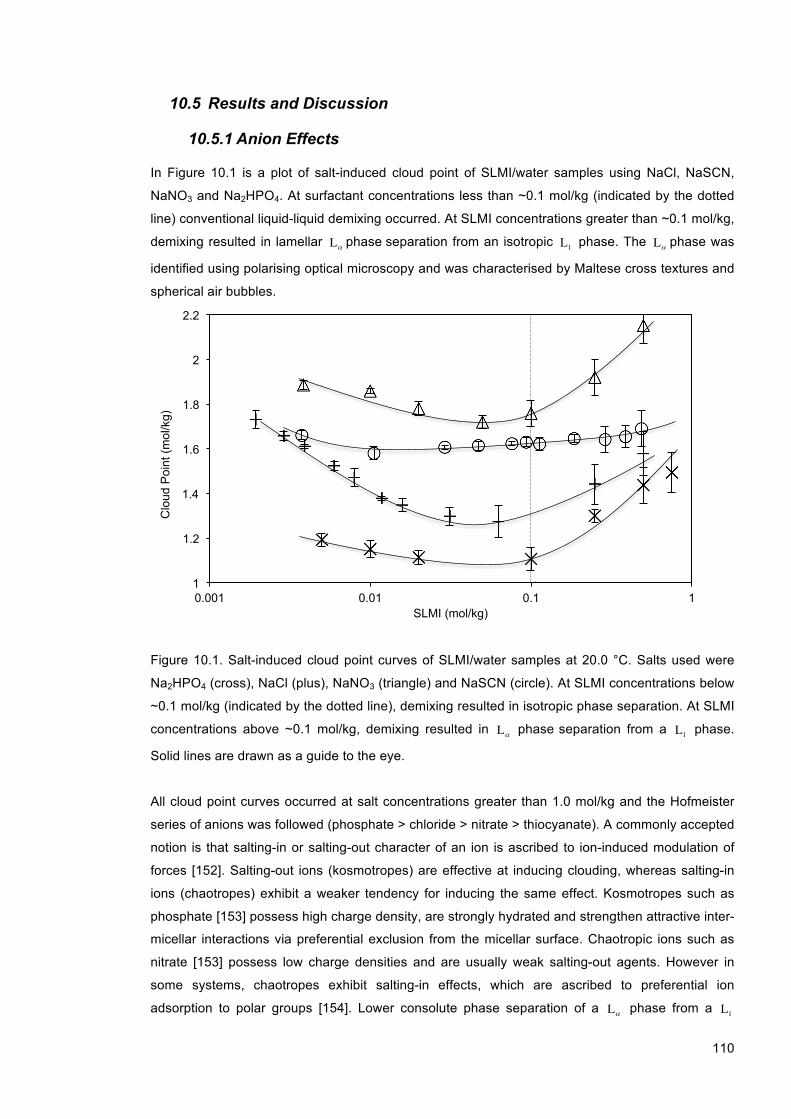
110


10.5.1 Anion Effects

In Figure 10.1 is a plot of salt-induced cloud point of SLMI/water samples using NaCl, NaSCN,

NaNO3 and Na2HPO4. At surfactant concentrations less than ~0.1 mol/kg (indicated by the dotted

line) conventional liquid-liquid demixing occurred. At SLMI concentrations greater than ~0.1 mol/kg,

demixing resulted in lamellar Lα phase separation from an isotropic L1 phase. The Lα phase was

identified using polarising optical microscopy and was characterised by Maltese cross textures and

spherical air bubbles.

Figure 10.1. Salt-induced cloud point curves of SLMI/water samples at 20.0 °C. Salts used were

Na2HPO4 (cross), NaCl (plus), NaNO3 (triangle) and NaSCN (circle). At SLMI concentrations below

~0.1 mol/kg (indicated by the dotted line), demixing resulted in isotropic phase separation. At SLMI

concentrations above ~0.1 mol/kg, demixing resulted in Lα phase separation from a L1 phase.

Solid lines are drawn as a guide to the eye.

All cloud point curves occurred at salt concentrations greater than 1.0 mol/kg and the Hofmeister

series of anions was followed (phosphate > chloride > nitrate > thiocyanate). A commonly accepted

notion is that salting-in or salting-out character of an ion is ascribed to ion-induced modulation of

forces [152]. Salting-out ions (kosmotropes) are effective at inducing clouding, whereas salting-in

ions (chaotropes) exhibit a weaker tendency for inducing the same effect. Kosmotropes such as

phosphate [153] possess high charge density, are strongly hydrated and strengthen attractive inter-

micellar interactions via preferential exclusion from the micellar surface. Chaotropic ions such as

nitrate [153] possess low charge densities and are usually weak salting-out agents. However in

some systems, chaotropes exhibit salting-in effects, which are ascribed to preferential ion

adsorption to polar groups [154]. Lower consolute phase separation of a Lα phase from a L1

1

1.2

1.4

1.6

1.8

2

2.2

0.001 0.01 0.1 1

Clo

ud P

oint

(mol

/kg)

SLMI (mol/kg)

111

phase may provide an indication of micelle structure at the cloud point. Since it is established that

the Lα phase comprises bilayers [6], it may be possible that micelles exists as flat bilayer disks at

cloud point compositions. In Figure 10.2 are plots of micelle (a) hydrodynamic diamter dH (DLS),

(b) polydispersity index χ (DLS) and (c) photon count rate φ (SLS) as a function of salt

concentration in SLMI/water samples. The salts tested were Na2HPO4 (cross), NaCl (plus), NaNO3

(triangle) and NaSCN (circle). Marked increases in dH , φ and χ were observed as a function of

increasing salt concentration.

(a) (b)

(c)

Figure 10.2. Plots of (a) hydrodynamic diameter dH , (b) polydispersity index χ and (c) count rate

φ of micelles as a function of salt concentration prior to the cloud point in SLMI/water samples (0.1

mol/kg). The salts used were Na2HPO4 (cross), NaCl (plus), NaNO3 (triangle) and NaSCN (circle).

All experiments were conducted at 20.0 °C. Lines are drawn as a guide to the eye.

0

50

100

150

200

250

0 0.5 1 1.5 2

Hyd

rody

nam

ic D

iam

eter

(nm

)

Salt (mol/kg)

0

0.2

0.4

0.6

0.8

1

0 0.5 1 1.5 2

Pol

ydis

pers

ity

Salt (mol/kg)

0

10000

20000

30000

40000

50000

60000

70000

0 0.2 0.4 0.6 0.8 1 1.2 1.4 1.6 1.8

Cou

nt R

ate

(kcp

s)

Salt (mol/kg)

112

The changes in Hd , χ and φ as a function of added salt are primarily attributed to changes in

micelle geometry. As the salt concentration approaches 0.1 mol/kg, micelle surface charge is

screened and the Debye length approaches ~1 nm [10]; electrostatic contributions are minimised to

negligible levels. For all salts tested, Hd , χ and ϕ continually increased beyond ~0.1 mol/kg,

implying that a cloud point mechanism based on DLVO-type electrostatic interactions may be ruled

out. An additional interaction that occurs at salt concentrations greater than 1 mol/kg is surface

dehydration of the micelle, which is due to a reduction in water activity. Micelle surface dehydration

facilitates a micelle shape change to a more favourable structure via reducing the average head

group area in the micelle. Changes in micelle size as a function of added salt were consistent in

both sets of light scattering data. As salt concentration is further increased the micelles eventually

increase to maximum size and reflect peak values in ϕ and Hd . For NaCl and NaHPO4, Hd and ϕ

exhibit a subsequent decrease after the peak values. A possible explanation is due to a reduction

in micelle size from the break-up of long rod-like micelles into smaller flat disc micelles. Our results

share similarities with SANS studies on conventional temperature-induced cloud points of a non-

ionic surfactant system conducted by Glatter et al., who provided strong evidence to indicate a

micelle growth mechanism followed by an attractive intermicellar potential at the cloud point [155].

Alternatively, the result may be due to intersection of the spinodal, which would originate from

slight error in cloud point measurement. Spinodal decomposition could potentially lead to material

settlement and a reduction in light scattering intensity.

10.5.2 Cation Effects

Cation specific interactions with surfactant micelles were probed by measuring salt-induced cloud

point/precipitation point curves of SLMI/water samples using a range of chloride salts. Experiments

were performed to probe cation specific interactions with surfactant micelles. Addition of KCl to

SLMI/water solutions resulted in precipitation of an insoluble solid phase. NaCl, LiCl and NH4Cl

addition yielded separation of either a Lα phase from a L1 phase (greater than approximately 0.1

mol/kg SLMI) or L1 phase separation (less than approximately 0.1 mol/kg SLMI). In Figure 10.3 are

plots of salt-induced cloud points and precipitation points in SLMI/water samples. The salts tested

were NaCl (triangle), NH4Cl (cross), KCl (plus) and LiCl (circle). NH4Cl exhibited a greater salting

out potency than LiCl, as indicated by its effect at inducing lower salt concentration cloud points.

113

Figure 10.3. Salt-induced precipitation/cloud point curves of SLMI/water samples at 20.0 °C. The

salts used were NH4Cl (cross), KCl (plus), LiCl (circle) and NaCl (triangle). At SLMI/water

compositions below ~0.1 mol/kg (indicated by the dotted line) demixing resulted in L1 phase

separation. At SLMI/water concentrations above ~0.1 mol/kg, demixing resulted in Lα phase

separation from a L1 phase. Solid lines are drawn as a guide to the eye.

Precipitation of a solid surfactant phase may occur on intersecting the Krafft boundary [11].

According to Collins [156], oppositely charged functional groups with similar water affinities form

close proximity ion pairs. Ion pairing is a process that decreases surfactant solubility and results in

precipitation if ion binding is sufficiently strong. The sulfonate head group of SLMI exhibits a strong

affinity for the potassium ion, as indicated by a precipitation point curve at low KCl concentrations.

KCl-induced precipitation implies that potassium strongly binds to the sulfonate head group of

SLMI, yielding formation of an insoluble potassium salt. Our results are in agreement with

experiments conducted by Terabe et al. [157], who report the Krafft temperature of potassium

dodecyl sulphate (~35 °C) to be higher than that of sodium dodecyl sulphate (~16 °C). A

particularly key observation is that most KCl-induced precipitation points occur at salt

concentrations under 0.1 mol/kg KCl [134]. The occurrence of a precipitation point curve at

electrolyte concentrations under ~0.1 mol/kg indicates that electrostatic effects are significant,

which supports the mechanistic explanation of close proximity ion binding.

In Figure 10.4 are plots of SLMI/water (0.1 mol/kg) micelle properties ((a) dH (DLS), (b) χ (DLS)

and (c) φ (SLS)) as a function of salt concentration prior to the cloud point. The salts used were

NH4Cl (cross) and LiCl (triangle) and NaCl (circle). Light scattering data for KCl are not shown, as

samples were too low in ionic strength to obtain reliable data. Increasing salt concentration

generally yielded increases in dH and φ . For LiCl and NH4Cl, χ remained fairly unchanged as a

function of increasing salt concentration.

0

0.5

1

1.5

2

2.5

3

0.001 0.01 0.1 1

Pre

cipi

tatio

n/C

loud

Poi

nt (m

ol/k

g)

SLMI (mol/kg)

114

(a) (b)

(c)

Figure 10.4. Plots of (a) hydrodynamic diameter dH , (b) polydispersity index χ and (c) count rate

φ of micelles as a function of salt concentration in SLMI/water samples. The salts used were

NH4Cl (cross) and LiCl (triangle) and NaCl (circle). All experiments were conducted using SLMI

(0.1 mol/kg) at 20.0 °C. Lines are drawn as a guide to the eye.

The increases in dH , χ and φ as a function of salt concentration are attributed primarily to

increases in micelle size. Due to the opposite charge of the cation and SLMI head group,

interactions are expected to be ion specific at concentrations where electrostatic effects dominate.

However, as the salt concentration is significantly above the screening level, electrostatic effects

are negligible and a cloud point mechanism involving surface dehydration and ion adsorption is

expected to apply.

0

20

40

60

80

100

120

140

160

180

0 0.3 0.6 0.9 1.2 1.5 1.8 2.1 2.4

Hyd

rody

nam

ic D

iam

eter

[nm

]

Salt (mol/ kg)

0

0.2

0.4

0.6

0.8

1

1.2

0 0.5 1 1.5 2 2.5

Pol

ydis

pers

ity In

dex

Salt (mol/kg)

0

10000

20000

30000

40000

50000

60000

70000

0 0.3 0.6 0.9 1.2 1.5 1.8 2.1 2.4

Cou

nt R

ate

(kcp

s)

Salt (mol/kg)

115

10.5.3 Salt-Induced Cloud Point Mechanism

Salting out anions raise the chemical potential of surfactant micelles, which consequently become

unstable at increased salt concentrations [158]. As the micelle chemical potential exceeds a critical

value, micelle-micelle fusion results, inducing cloudiness and subsequent demixing of a surfactant

rich phase from a surfactant depleted phase. Micelle fusion is thought to occur due to an induced

electrostatic image force at high salt concentration. Image forces cause the net exclusion of ions

from the micelle surface [154, 159-161], as ions prefer to be in an electrostatically screened

environment away from the low dielectric surface of micelles [162, 163]. As a consequence, the

region of ion exclusion invokes depletion forces between micelles. As salt concentration surpasses

a particular value, the magnitude of depletion forces is sufficiently strong to induce micelle-micelle

fusion, which is visually observable from solution clouding. In addition, we speculate that the close

proximity of the lamellar phase boundary to the cloud point implies a flat disk-like micelle geometry

[6, 10].

Ion specificity has been analysed by comparing cloud point curves to salt-induced surface tension

increments (dγ/dc) of the respective salt. In Table 10.1 are shown dγ/dc values at the air-water

interface for some of the salts tested.

Table 10.1. Salt-induced surface tension increment and calculated surface tension increments at

the cloud point at 20.0 °C for NaNO3[164], NH4Cl [165], LiCl[34], NaCl[166], NaSCN[167] and

Na2HPO4 [168].

Salt dγ/dc (mN.kg/m.mol) dγ (γcloud point – γpure water) (mN/m) NaNO3 1.06 1.82 NH4Cl 1.23 1.94 LiCl 1.42 3.48 NaCl 1.46 1.83

NaSCN 0.57 0.90 Na2HPO4 2.02 2.22

On comparison of dγ/dc data in Table 10.1 with the cloud point curves in Figure 10.1 and 10.3, one

may conclude that the salt-induced changes in surface tension generally scale with the

experimentally determined ordering of cloud points for the ions. As a consequence, there is some

evidence to suggest that the cloud point mechanism may be related to changes in surface tension,

which are linked to electrostatic image forces. Na2HPO4 has the largest dγ/dc value (2.02) and

therefore induces the strongest exclusion effect. Consequently, Na2HPO4 is the most effective of

tested electrolytes at salting out. Cloud point curve positions were generally in agreement with the

data.

Variations in the data presented may originate from the high impurity/process component

concentration in SLMI (~15 % (w/w). See Section 6.2), which could induce additional interactions

that affect cloud point curves. A clear limitation of analysing the data in terms of dγ/dc values of the

116

air-water interface is that the micelle surface-salt solution interface is non-equivalent. Only

qualitative comparisons can be made.


Salting-out causes the cloud point to occur in the sodium lauroyl methyl isethionate/ water system

and the Hofmeister series for anions was generally followed. Our static and dynamic light scattering

data supports theories linking the salting-out interaction to depletion forces. The trend in light

scattering count rate and hydrodynamic diameter as a function of added salt provides an indicator

of micelle geometry before the cloud point. We noticed for some salts there was a drop in light

scattering signal intensity immediately before clouding, which could imply a rod-to-disc micelle

shape transition. The result needs validating using an independent experiment, such as obtaining

solution viscosity measurements for the same samples.

A point of discussion is the behaviour of lithium chloride. The LiCl-induced cloud point curve of

SLMI/water solutions is above 2 mol/kg salt, meaning it is unlikely that lithium binds to the sulfonate

head group of SLMI. Lithium salts are expected to exhibit strong salting-out effects on non-polar

groups, as water molecules heavily hydrate the lithium ion. However, lithium salts generally exhibit

weak salting out effects on non-polar groups [169]. The anomalous effects of lithium provide strong

evidence that charge density alone cannot rationalise Hofmeister behaviour. Thomas et al.

simulated a number of Hofmeister salts in aqueous solvent and their results indicated that LiCl

solvates as alternating “strings” of Li+ and Cl- ions. The authors concluded that unusual effects of

LiCl were not due to direct interactions between Li+ and hydrophobic solutes, but were instead due

to LiCl-induced solvent effects.

Future experiments will involve conducting rheological experiments on SLMI/water solutions at salt

concentrations prior to the cloud point. The dependence of solution viscosity on salt concentration

(before the cloud point) would validate previous results. We would expect to observe a decrease in

viscosity on transitioning from rod to disk shaped micelles.

117

11 Research Summary In Chapter 7 we utilised a combination of polarising optical microscopy, differential scanning

calorimetry and x-ray diffraction techniques to characterise SLMI/water phase behaviour across a

specified temperature range. A temperature-composition phase diagram was constructed. The

information provides useful information on the aqueous phase behaviour of SLMI and a basis for

future investigations into the effects of additional formulation components such as alcohols,

electrolytes, secondary surfactants and fragrances.

Rheology and light scattering techniques were utilised in Chapter 8 to determine the effects of

synthesis-derived components on the viscosity of a base formulation (SLMI/sodium {(3-

(dodecanoylamino)propyl)(dimethyl)ammonio)}acetate/water). Our study included the most

abundant ((w/w) %) synthesis derived components in SLMI: propylene glycol dilaurate, sodium

methyl isethionate and lauric acid. Experimental observations were rationalised by considering

micelle geometry and the critical packing parameter. Our research provides the first step towards

determining qualitative relationships between formulation viscosity and component concentration.

Chapter 9 reports an initial study of the micelle build-up process on mixing aqueous components of

SLMI and (carboxylatomethyl)hexadecyldimethyl ammonium. Our study utilises nuclear magnetic

resonance spectroscopy and light scattering to characterise micelle growth as a function of

surfactant concentration and surfactant mass fraction. The results improve our understanding of

micelle growth, however further experiments need to be performed before a mechanism can be

suggested. Micelle break-down complicates the growth process and needs to be investigated using

the analogous experimental techniques. Experimental data on both build-up and break-down

processes will improve our understanding of non-equilibrium micelle kinetics.

In the final Chapter we report a study on salt-induced cloud point behaviour in the SLMI/water

system. Cloud point curves were determined via turbidimetry measurements for a range of sodium-

and chloride- salts. The micellar properties of SLMI/”salt”/water samples were characterised as a

function of salt concentration prior to the cloud point. Our results follow the Hofmeister series of

anions and support previous theories linking micelle clouding to electrolyte-induced depletion

forces. Future experiments will include performing an independent rheological study for

comparison.

118

12 References [1] J. H. Clint, Surfactant Aggregation: Blackie, 1992. [2] J. Texter, Reactions and Synthesis in Surfactant Systems: Marcel Dekker

Incorporated, 2001. [3] M. J. Rosen, Surfactants and Interfacial Phenomena: Wiley-Interscience, 2004. [4] G. Scatchard, "Gibbs Adsorption Isotherm," Journal of Physical Chemistry, vol. 66,

pp. 618-&, 1962. [5] D. F. Evans and H. Wennerstrom, The Colloidal Domain: Where Physics,

Chemistry, Biology and Technology Meet: Wiley, 1999. [6] S. Hassan, W. Rowe, and G. J. T. Tiddy, "Surfactant Liquid Crystals," Handbook of

Applied Surface and Colloid Chemistry, vol. 21, pp. 465-503, 2001. [7] H. J. Butt, K. Graf, and M. Kappl, Physics and Chemistry of Interfaces: John Wiley

& Sons, 2006. [8] J. Iyer and D. Blankschtein, "Are Ellipsoids Feasible Micelle Shapes? An Answer

Based on a Molecular-Thermodynamic Model of Nonionic Surfactant Micelles," The Journal of Physical Chemistry B, vol. 116, pp. 6443-6454, 2012/06/07 2012.

[9] C. Tanford, "Micelle Shape and Size," The Journal of Physical Chemistry, vol. 76, pp. 3020-3024, 1972/10/01 1972.

[10] J. N. Israelachvili, Intermolecular And Surface Forces: Academic Press, 2010. [11] R. G. Laughlin, The Aqueous Phase Behavior of Surfactants: Academic press,

1996. [12] P. Alexandridis and T. Alan Hatton, "Poly(ethylene oxide)-poly(propylene oxide)-

poly(ethylene oxide) Block Copolymer Surfactants in Aqueous Solutions and at Interfaces: Thermodynamics, Structure, Dynamics, and Modeling," Colloids and Surfaces A: Physicochemical and Engineering Aspects, vol. 96, pp. 1-46, 3/10/ 1995.

[13] P. M. S. Monk, Physical Chemistry: Understanding our Chemical World: Wiley, 2008.

[14] J. M. Corkill, J. F. Goodman, T. Walker, and J. Wyer, "The Multiple Equilibrium Model of Micelle Formation," Proceedings of the Royal Society of London. Series A, Mathematical and Physical Sciences, vol. 312, pp. 243-255, 1969.

[15] E. Aniansson and S. Wall, "Kinetics of Step-wise Micelle Association. Correction and Improvement," Journal of Physical Chemistry, vol. 79, pp. 857-858, 1975.

[16] J. Rassing, P. Sams, and E. Wyn-Jones, "Kinetics of Micellization from Ultrasonic Relaxation Studies," Journal of the Chemical Society, Faraday Transactions 2: Molecular and Chemical Physics, vol. 70, pp. 1247-1258, 1974.

[17] E. Aniansson, S. Wall, M. Almgren, H. Hoffmann, I. Kielmann, W. Ulbricht, et al., "Theory of the Kinetics of Micellar Equilibria and Quantitative Interpretation of Chemical Relaxation Studies of Micellar Solutions of Ionic Surfactants," The Journal of Physical Chemistry, vol. 80, pp. 905-922, 1976.

[18] T. Okubo, H. Kitano, T. Ishiwatari, and N. Ise, "Conductance Stopped-Flow Study on the Micellar Equilibria of Ionic Surfactants," Proceedings of the Royal Society of London. A. Mathematical and Physical Sciences, vol. 366, pp. 81-90, 1979.

[19] S. Kato, H. Nomura, H. Honda, R. Zielinski, and S. Ikeda, "Ultrasonic Relaxation Study of the Exchange Process of Surfactant Monomer with Micelle in Aqueous Solutions of Alkyltrimethylammonium Bromides," The Journal of Physical Chemistry, vol. 92, pp. 2305-2310, 1988/04/01 1988.

[20] H. Walderhaug, O. Soederman, and P. Stilbs, "Micellar Dynamics and Organization. A Multifield Carbon-13 NMR Spin-Lattice Relaxation and {Proton} Carbon-13 Nuclear Overhauser Effect Study," The Journal of Physical Chemistry, vol. 88, pp. 1655-1662, 1984/04/01 1984.

[21] B. Lindman, "Structural Aspects of Surfactant Micellar Systems," in Surfactants, T. F. Tadros, Ed., ed: Academic Press, 1984, p. 83.

[22] Y. Shao and T. Zerda, "Phase Transitions of Liquid Crystal PAA in Confined Geometries," The Journal of Physical Chemistry B, vol. 102, pp. 3387-3394, 1998.

[23] E. Lueder, Liquid Crystal Displays: Addressing Schemes and Electro-Optical Effects: Wiley, 2010.

119

[24] V. R. Horowitz, L. A. Janowitz, A. L. Modic, P. A. Heiney, and P. J. Collings, "Aggregation Behavior and Chromonic Liquid Crystal Properties of an Anionic Monoazo Dye," Physical Review E, vol. 72, p. 041710, 2005.

[25] E. Jurado, V. Bravo, J. M. Vicaria, A. Fernandez-Arteaga, and A. I. Garcia-Lopez, "Triolein Solubilization Using Highly Biodegradable Non-Ionic Surfactants," Colloids and Surfaces A: Physicochemical and Engineering Aspects, vol. 326, pp. 162-168, 2008.

[26] K. Rendall, G. J. T. Tiddy, and M. A. Trevethan, "Optical Microscopy and Nuclear Magnetic Resonance Studies of Mesophases Formed at Compositions Between Hexagonal and Lamellar Phases in Sodium N-Alkanoate + Water Mixtures and Related Surfactant Systems," Journal of the Chemical Society, Faraday Transactions 1: Physical Chemistry in Condensed Phases, vol. 79, pp. 637-649, 1983.

[27] P. Sakya, J. M. Seddon, R. H. Templer, R. J. Mirkin, and G. J. T. Tiddy, "Micellar Cubic Phases and their Structural Relationships: The Nonionic Surfactant System C12EO12/Water," Langmuir, vol. 13, pp. 3706-3714, Jul 9 1997.

[28] J. M. Seddon, E. A. Bartle, and J. Mingins, "Inverse Cubic Liquid-Crystalline Phases of Phospholipids and Related Lyotropic Systems " Journal of Physics: Condensed Matter, vol. 2, 1990.

[29] A. Gulik, H. Delacroix, G. n. Kirschner, and V. Luzzati, "Polymorphism of Ganglioside-Water Systems: a New Class of Micellar Cubic Phases. Freeze-Fracture Electron Microscopy and X-Ray Scattering Studies," J. Phys. II France, vol. 5, pp. 445-464, 1995.

[30] J. Charvolin and J. F. Sadoc, "Periodic Systems of Frustrated Fluid Films and Micellar Cubic Structures in Liquid Crystals," Journal of Physics, vol. 49, pp. 521-526, 1988.

[31] J. M. Seddon, "Structure of the Inverted Hexagonal (HII) Phase, and Non-Lamellar Phase Transitions of Lipids," Biochimica et Biophysica Acta, vol. 1031, pp. 1-69, 1990.

[32] J. M. Seddon and R. H. Templer, Structure and Dynamics of Membranes: From Cells to Vesicles vol. 1. Amsterdam: Elsevier, 1995.

[33] G. Lindblom and L. Rilfors, "Cubic Phases and Isotropic Structures Formed by Membrane-Lipids - Possible Biological Relevance," Biochimica et Biophysica Acta, vol. 988, pp. 221-256, May 1989.

[34] K. Fontell, K. K. Fox, and E. Hansson, "On the Structure of the Cubic Phase in some Lipid-Water Systems," Molecular Crystals and Liquid Crystals, vol. 1, pp. 9-17, 1985.

[35] L. E. Scriven, "Equilibrium Bicontinuous Structure," Nature, vol. 263, pp. 123-125, 1976.

[36] K. D. Lawson and T. J. Flautt, "Magnetically Oriented Lyotropic Liquid Crystalline Phases," Journal of the American Chemical Society, vol. 89, pp. 5489-&, 1967.

[37] J. Nehring and A. Saupe, "On the Schlieren Texture in Nematic and Smectic Liquid Crystals," Journal of the Chemical Society, Faraday Transactions 2: Molecular and Chemical Physics, vol. 68, pp. 1-15, 1972.

[38] B. J. Forrest and L. W. Reeves, "New Lyotropic Liquid-Crystals Composed of Finite Nonspherical Micelles," Chemical Reviews, vol. 81, pp. 1-14, 1981.

[39] N. Boden, P. H. Jackson, K. McMullen, and M. C. Holmes, "Are Nematic Amphiphilic Liquid-Crystalline Mesophases Thermodynamically Stable?," Chemical Physics Letters, vol. 65, pp. 476-479, 1979.

[40] L. A. Madsen, T. J. Dingemans, M. Nakata, and E. T. Samulski, "Thermotropic Biaxial Nematic Liquid Crystals," Physical Review Letters, vol. 92, p. 145505, 04/09/ 2004.

[41] G. S. Smith, E. B. Sirota, C. R. Safinya, R. J. Plano, and N. A. Clark, "X-Ray Structural Studies of Freely Suspended Ordered Hydrated DMPC Multimembrance Films," Journal of Chemical Physics, vol. 92, pp. 4519-4529, Apr 1990.

[42] J. Katsaras, "Structure Of The Subgel and Gel Phases of Oriented Dipalmitoylphosphatidylcholine Multibilayers," Journal of Physical Chemistry, vol. 99, pp. 4141-4147, Mar 1995.

[43] D. Chapman, R. M. Williams, and B. D. Ladbrooke, "Physical Studies of Phospholipids. Vi. Thermotropic and Lyotropic Mesomorphism of some 1,2-Diacyl-

120

Phosphatidylcholines (Lecithins)," Chemistry and Physics of Lipids, vol. 1, pp. 445-475, 1967.

[44] K. Larsson, "Structure Of Mesomorphic Phases and Micelles in Aqueous Glyceride Systems," Zeitschrift Fur Physikalische Chemie-Frankfurt, vol. 56, pp. 173-&, 1967.

[45] J. M. Vincent and A. Skoulios, "Gel and Coagel. 1. Indentification. Location in a Phase Diagram and Determining the Structure of the Gel in the case of Potassium Stearate," Acta Crystallographica, vol. 20, p. 432, 1966.

[46] H. Hagslätt, O. Söderman, and B. Jönsson, "The Structure of Intermediate Ribbon Phases in Surfactant Systems," Liquid Crystals, vol. 12, pp. 667-688, 1992/10/01 1992.

[47] C. E. Fairhurst, M. C. Holmes, and M. S. Leaver, "Structure And Morphology of the Intermediate Phase Region in the Nonionic Surfactant C16Eo6/Water System," Langmuir, vol. 13, pp. 4964-4975, Sep 1997.

[48] C. E. Fairhurst, M. C. Holmes, and M. S. Leaver, "Shear Alignment of a Rhombohedral Mesh Phase in Aqueous Mixtures of a Long Chain Nonionic Surfactant," Langmuir, vol. 12, pp. 6336-6340, Dec 1996.

[49] D. J. Mitchell, G. J. T. Tiddy, L. Waring, T. Bostock, and M. P. McDonald, "Phase Behaviour of Polyoxyethylene Surfactants with Water. Mesophase Structures and Partial Miscibility (Cloud Points)," Journal of the Chemical Society, Faraday Transactions 1: Physical Chemistry in Condensed Phases, vol. 79, pp. 975-1000, 1983.

[50] P. Somasundaran, Encyclopedia of Surface and Colloid Science: Taylor & Francis, 2006.

[51] W. Kunz, J. Henle, and B. W. Ninham, "About the Science of the Effect of Salts: Franz Hofmeister's Historical Papers," Current Opinion in Colloid & Interface Science, vol. 9, pp. 19-37, 2004.

[52] W. Kunz, "Specific Ion Effects in Colloidal and Biological Systems," Current Opinion in Colloid & Interface Science, vol. 15, pp. 34-39, 2010.

[53] K. D. Collins, G. W. Neilson, and J. E. Enderby, "Ions in Water: Characterizing the Forces that Control Chemical Processes and Biological Structure," Biophysical Chemistry, vol. 128, pp. 95-104, 7// 2007.

[54] B. Jagoda-Cwiklik, R. Vácha, M. Lund, M. Srebro, and P. Jungwirth, "Ion Pairing as a Possible Clue for Discriminating between Sodium and Potassium in Biological and Other Complex Environments," The Journal of Physical Chemistry B, vol. 111, pp. 14077-14079, 2007/12/01 2007.

[55] L. Vrbka, J. Vondrášek, B. Jagoda-Cwiklik, R. Vácha, and P. Jungwirth, "Quantification and Rationalization of the Higher Affinity of Sodium Over Potassium to Protein Surfaces," Proceedings of the National Academy of Sciences, vol. 103, pp. 15440-15444, October 17, 2006 2006.

[56] N. Vlachy, B. Jagoda-Cwiklik, R. Vácha, D. Touraud, P. Jungwirth, and W. Kunz, "Hofmeister Series and Specific Interactions of Charged Headgroups with Aqueous Ions," Advances in Colloid and Interface Science, vol. 146, pp. 42-47, 2/28/ 2009.

[57] P. Ekwall, "Composition, Properties and Structures of Liquid Crystalline Phases in Systems of Amphiphilic Compounds," in Advances in Liquid Crystals. vol. Volume 1, H. B. Glenn, Ed., ed: Elsevier, 1975, pp. 1-142.

[58] K. Holmberg and B. Jönsson, Surfactants and Polymers in Aqueous Solution: John Wiley & Sons, 2003.

[59] I. Dierking, Textures of Liquid Crystals: Wiley, 2006. [60] S. T. Hyde, "Identification of Lyotropic Liquid Crystalline Mesophases," Handbook

of Applied Surface and Colloid Chemistry, pp. 299-332, 2001. [61] T. Scharf, Polarized Light in Liquid Crystals and Polymers: Wiley, 2007. [62] H. F. Gleeson, "The Physics of Liquid Crystals," presented at the BLCS Workshop,

Hull, 2003. [63] E. Pungor and G. Horvai, A Practical Guide to Instrumental Analysis: Taylor &

Francis, 1994. [64] R. G. Mortimer, Physical Chemistry: Elsevier Science, 2008. [65] B. Andersson and G. Olofsson, "Differential Scanning Calorimetric Study of Phase

Changes in Poly(Ethylene Glycol) Dodecyl Ether-Water Systems," Colloid and Polymer Science, vol. 265, pp. 318-328, 1987/04/01 1987.

[66] R. G. Larson, The Structure and Rheology of Complex Fluids: OUP USA, 1999.

121

[67] R. Zana, Dynamics of Surfactant Self-Assemblies: Micelles, Microemulsions, Vesicles and Lyotropic Phases: Taylor & Francis, 2005.

[68] H. F. Brinson and L. C. Brinson, Polymer Engineering Science and Viscoelasticity: An Introduction: Springer, 2007.

[69] S. Kumar, Liquid Crystals: Experimental Study of Physical Properties and Phase Transitions: Cambridge University Press, 2001.

[70] A. R. West, Solid State Chemistry and its Applications: Wiley, 2014. [71] C. Suryanarayana and G. Norton, X-Ray Diffraction: A Practical Approach:

Springer, 1998. [72] I. W. Hamley, Introduction to Soft Matter: Synthetic and Biological Self-Assembling

Materials: Wiley, 2013. [73] V. Luzzati and F. Husson, "The Structure of the Liquid-Crystalline Phases of Lipid-

Water Systems," The Journal of cell biology, vol. 12, pp. 207-219, 1962. [74] B. J. Berne and R. Pecora, Dynamic Light Scattering: With Applications to

Chemistry, Biology, and Physics: Dover Publications, 2000. [75] K. S. Schmitz, An Introduction to Dynamic Light Scattering by Macromolecules:

Academic Press, 1990. [76] P. C. Hiemenz and R. Rajagopalan, Principles of Colloid and Surface Chemistry,

Third Edition, Revised and Expanded: Taylor & Francis, 1997. [77] W. Brown, Dynamic Light Scattering: The Method and Some Applications:

Clarendon Press, 1993. [78] B. H. Zimm, "The Scattering of Light and the Radial Distribution Function of High

Polymer Solutions," The Journal of Chemical Physics, vol. 16, pp. 1093-1099, 1948.

[79] K. Khougaz, Z. Gao, and A. Eisenberg, "Determination of the Critical Micelle Concentration of Block Copolymer Micelles by Static Light Scattering," Macromolecules, vol. 27, pp. 6341-6346, 1994.

[80] O. Söderman, P. Stilbs, and W. S. Price, "NMR Studies of Surfactants," Concepts in Magnetic Resonance Part A, vol. 23, pp. 121-135, 2004.

[81] J. W. Akitt and B. E. Mann, NMR and Chemistry: An Introduction to Modern NMR Spectroscopy, 4 ed.: Taylor & Francis, 2000.

[82] B. Cowan, Nuclear Magnetic Resonance and Relaxation: Cambridge University Press, 2005.

[83] M. Bruch, NMR Spectroscopy Techniques, Second Edition: Taylor & Francis, 1996.

[84] D. Pavia, G. Lampman, G. Kriz, and J. Vyvyan, Introduction to Spectroscopy: Cengage Learning, 2014.

[85] M. Popov, Modern NMR Techniques and Their Application in Chemistry: Taylor & Francis, 1990.

[86] H. Friebolin, Basic One- and Two-Dimensional NMR Spectroscopy: John Wiley & Sons, 2005.

[87] J. Christer, U. Henriksson, and L. Odberg, "NMR-Studies on Molecular Movement of Micelles and Floating Crystals," Kemisk Tidskrift, vol. 89, pp. 40-&, 1977.

[88] G. S. Rule and T. K. Hitchens, Fundamentals of Protein NMR Spectroscopy: Springer, 2006.

[89] G. J. T. Tiddy and A. Wheeler, "The Kinetics of Formation and Breakdown of Pre-Hexagonal Phase Aggregates in Fluid-Isotropic Amphiphile Solutions," J. Phys. Colloques, vol. 36, pp. 167-172, 1975.

[90] P. Somasundaran, Encyclopedia of Surface and Colloid Science: Taylor & Francis, 2006.

[91] I. Furó, "NMR Spectroscopy of Micelles and Related Systems," Journal of Molecular Liquids, vol. 117, pp. 117-137, 3/15/ 2005.

[92] E. J. Staples and G. J. T. Tiddy, "Nuclear Magnetic Resonance Technique to Distinguish Between Micelle Size Changes and Secondary Aggregation in Anionic and Nonionic Surfactant Solutions," Journal of the Chemical Society, Faraday Transactions 1: Physical Chemistry in Condensed Phases, vol. 74, pp. 2530-2541, 1978.

[93] P. A. Wheeler and G. J. T. Tiddy, "Non-Equilibrium Properties of Viscoelastic Surfactant Solutions," Unpublished, 1978.

122

[94] G. A. Morris and J. W. Emsley, Multidimensional NMR Methods for the Solution State: Wiley, 2012.

[95] S. X. Liu and J.-T. Kim, "Study of Adsorption Kinetics of Surfactants onto Polyethersulfone Membrane Surface using QCM-D," Desalination, vol. 247, pp. 355-361, 10// 2009.

[96] J. A. Zimmerman and R. L. Schnaare, "Predicting the Critical Micelle Concentration in a pH-Mediated Ternary-Surfactant Mixture Using the Regular Solution Approximation," Journal of Colloid and Interface Science, vol. 220, pp. 75-80, 12/1/ 1999.

[97] C. L. Richards, "Mixed Surfactant Mesophases for Improved Product Processing and Dispersion," School of Chemical Engineering and Analytical Science, University of Manchester, 2005.

[98] T. C. Huang, H. Toraya, T. N. Blanton, and Y. Wu, "X-Ray Powder Diffraction Analysis of Silver Behenate, a Possible Low-Angle Diffraction Standard," Journal of Applied Crystallography, vol. 26, pp. 180-184, 1993.

[99] A. M. Bakr, T. Kawiak, M. Pawlikowski, and Z. Sawlowicz, "Characterisation of 15th Century Red and Black Pastes used for Wall Decoration in the Qijmas El-Eshaqi Mosque (Cairo, Egypt)," Journal of Cultural Heritage, vol. 6, pp. 351-356, 2005.

[100] S. Chandrasekhar, Liquid Crystals: Cambridge University Press, 1992. [101] M. C. Holmes and J. Charvolin, "Smectic Nematic Transition in a Lyotropic Liquid-

Crystal," Journal of Physical Chemistry, vol. 88, pp. 810-818, 1984 1984. [102] Y. Hendrikx, J. Charvolin, P. Kekicheff, and M. Roth, "Structural Fluctuations in

The Lamellar Phase of Sodium Decyl Sulfate Decanol Water," Liquid Crystals, vol. 2, pp. 677-687, Sep-Oct 1987.

[103] Y. Hendrikx, J. Charvolin, and M. Rawiso, "Segregation of 2 Amphiphilic Molecules Within Nonspherical Micelles - A Neutron-Scattering Study," Journal of Colloid and Interface Science, vol. 100, pp. 597-600, 1984 1984.

[104] P. Kekicheff and B. Cabane, "Crystallography of Systems with Long Periods - A Neutron-Scattering Study Of Sodium Dodecyl-Sulfate - Water Mesophases," Acta Crystallographica Section B-Structural Science, vol. 44, pp. 395-406, Aug 1988.

[105] N. Boden, S. A. Corne, and K. W. Jolley, "Lyotropic Mesomorphism of the Cesium Pentadecafluorooctanoate Water-System - High-Resolution Phase-Diagram," Journal of Physical Chemistry, vol. 91, pp. 4092-4105, Jul 16 1987.

[106] M. C. Holmes, J. Charvolin, and D. J. Reynolds, "An X-Ray-Scattering Study of the Lamellar Nematic Isotropic Sequence of Phases in Decylammonium Chloride H2O NH4Cl," Liquid Crystals, vol. 3, pp. 1147-1155, Aug 1988.

[107] M. S. Leaver and M. C. Holmes, "A Small-Angle Neutron-Scattering Study Of The Lamellar and Nematic Phases of Cesium Pentadecafluoro-Octanoate (CSPFO)/2H2O and CSPFO/CSCL/2H2O," Journal De Physique Ii, vol. 3, pp. 105-120, Jan 1993.

[108] S. S. Funari, M. C. Holmes, and G. J. T. Tiddy, "Microscopy, X-Ray-Diffraction and NMR Studies Of Lyotropic Liquid-Crystal Phases in The C22EO6/Water System - A New Intermediate Phase," Journal of Physical Chemistry, vol. 96, pp. 11029-11038, Dec 24 1992.

[109] M. Holmes, A. Smith, and M. Leaver, "A Small Angle Neutron Scattering Study of The Caesium Pentadecafluoro-Octanoate/2H2O and Two Associated Ternary Systems," Le Journal de Physique IV, vol. 3, pp. C8-177-C8-180, 1993.

[110] C. K. Bagdassarian, D. Roux, A. Ben-Shaul, and W. M. Gelbart, "Curvature Defects in Lamellar Phases of Amphiphile–Water Systems," The Journal of Chemical Physics, vol. 94, p. 3030, 1991.

[111] P. Kekicheff, C. Grabielle-Madelmont, and M. Ollivon, "Phase Diagram of Sodium Dodecyl Sulfate-Water System: 1. A Calorimetric Study," Journal of Colloid and Interface Science, vol. 131, pp. 112-132, 1989.

[112] M. Allain, "Possible Defect-Mediated Phase-Transition in a Lyotropic Liquid-Crystal - Electron-Microscopy Observations," Europhysics Letters, vol. 2, pp. 597-602, Oct 15 1986.

[113] P. Oswald and M. Allain, "Rheology and Structural Defects in a Lyotropic Lamellar Phase," Journal of Colloid and Interface Science, vol. 126, pp. 45-53, Nov 1988.

123

[114] S. Ozeki and S. Ikeda, "The Viscosity Behavior of Aqueous Nacl Solutions of Dodecyldimethylammonium Chloride and the Flexibility of its Rod-Like Micelle," Journal of Colloid and Interface Science, vol. 77, pp. 219-231, 1980.

[115] U. Kortemeier, J. Venzmer, A. Howe, B. Grüning, and S. Herrwerth, "Thickening Agents for Surfactant Systems," SÖFW Journal, vol. 136, p. 30, 2010.

[116] V. Hartmann and R. Cressely, "Simple Salt Effects on the Characteristics of the Shear Thickening Exhibited by an Aqueous Micellar Solution of CTAB/NaSal," EPL (Europhysics Letters), vol. 40, p. 691, 1997.

[117] U. Schilp, "Liquid, Thickened Chlorine Bleaching Composition," ed: Google Patents, 1982.

[118] V. G. Sonnen, "Hair and Scalp Treatment with a Principally Sodium Chloride Thick Viscous Aqueous Slurry," ed: Google Patents, 1971.

[119] H. Baust, "Extra Mild Shower Gel or Hair Shampoo Formulation," ed: Google Patents, 1992.

[120] H. Heerklotz, A. Tsamaloukas, K. Kita-Tokarczyk, P. Strunz, and T. Gutberlet, "Structural, Volumetric and Thermodynamic Characterization of a Micellar Sphere-to-Rod Transition," Journal of the American Chemical Society, vol. 126, pp. 16544-16552, 2004.

[121] L. Abezgauz, K. Kuperkar, P. A. Hassan, O. Ramon, P. Bahadur, and D. Danino, "Effect Of Hofmeister Anions on Micellization and Micellar Growth of the Surfactant Cetylpyridinium Chloride," Journal of Colloid and Interface Science, vol. 342, pp. 83-92, 2/1/ 2010.

[122] K. Y. Lai, Liquid Detergents: Taylor & Francis, 2005. [123] A. Desai, D. Varade, J. Mata, V. Aswal, and P. Bahadur, "Structural Transitions of

Cetyltrimethylammonium Bromide Micelles in Aqueous Media: Effect of Additives," Colloids and Surfaces A: Physicochemical and Engineering Aspects, vol. 259, pp. 111-115, 5/31/ 2005.

[124] P. Bahadur, K. Pandya, M. Almgren, P. Li, and P. Stilbs, "Effects of Inorganic Salts on the Micellar Behaviour of Ethylene Oxide-Propylene Oxide Block Copolymers in Aqueous Solution," Colloid and Polymer Science, vol. 271, pp. 657-667, 1993.

[125] G. C. Kalur and S. R. Raghavan, "Anionic Wormlike Micellar Fluids that Display Cloud Points:  Rheology and Phase Behavior," The Journal of Physical Chemistry B, vol. 109, pp. 8599-8604, 2005/05/01 2005.

[126] S. Kumar and A. Z. Naqvi, "Micellar Morphology in the Presence of Salts and Organic Additives," Langmuir, vol. 16, pp. 5252-5256, 2000.

[127] H. Iwata and K. Shimada, Formulas, Ingredients and Production of Cosmetics: Technology of Skin- and Hair-Care Products in Japan: Springer, 2012.

[128] M. Gradzielski, "Kinetics of Morphological Changes in Surfactant Systems," Current Opinion in Colloid & Interface Science, vol. 8, pp. 337-345, 11// 2003.

[129] A. Patist, J. R. Kanicky, P. K. Shukla, and D. O. Shah, "Importance of Micellar Kinetics in Relation to Technological Processes," Journal of Colloid and Interface Science, vol. 245, pp. 1-15, 1/1/ 2002.

[130] D. Saul, G. J. T. Tiddy, B. A. Wheeler, P. A. Wheeler, and E. Willis, "Phase Structure and Rheological Properties of a Mixed Zwitterionic-Anionic Surfactant System," Journal of the Chemical Society-Faraday Transactions I, vol. 70, pp. 163-170, 1974 1974.

[131] T. L. Hwang and A. J. Shaka, "Water Suppression That Works. Excitation Sculpting Using Arbitrary Wave-Forms and Pulsed-Field Gradients," Journal of Magnetic Resonance, Series A, vol. 112, pp. 275-279, 2// 1995.

[132] T. Iwasaki, M. Ogawa, K. Esumi, and K. Meguro, "Interactions Between Betaine-type Zwitterionic and Anionic Surfactants in Mixed Micelles," Langmuir, vol. 7, pp. 30-35, 1991/01/01 1991.

[133] C. Manohar, "Mechanism of the Clouding Phenomenon in Surfactant Solutions," in Adsorption and Aggregation of Surfactants in Solution, ed: CRC Press, 2002, pp. 211-217.

[134] P. Mukherjee, S. K. Padhan, S. Dash, S. Patel, and B. K. Mishra, "Clouding Behaviour in Surfactant Systems," Advances in Colloid and Interface Science, vol. 162, pp. 59-79, 2011.

[135] J. Goldfarb and L. Sepulveda, "Application of a Theory of Polymer Solutions to the Cloud Points of Nonionic Detergents," J Colloid Interfac Sci, vol. 31, p. 454, 1969.

124

[136] R. Kjellander, "Phase Separation of Non-ionic Surfactant Solutions. A Treatment of the Micellar Interaction and Form," Journal of the Chemical Society, Faraday Transactions 2: Molecular and Chemical Physics, vol. 78, pp. 2025-2042, 1982.

[137] V. Degiorgio and M. Corti, Physics of Amphiphiles: Micelles, Vesicles and Microemulsions: North-Holland, 1985.

[138] C. Tanford, Y. Nozaki, and M. F. Rohde, "Size and Shape of Globular Micelles Formed in Aqueous Solution by Normal-alkyl Polyoxyethylene Ethers," J Phys Chem, vol. 81, pp. 1555-1560, 1977.

[139] J. P. Conroy, C. Hall, C. A. Leng, K. Rendall, G. J. T. Tiddy, J. Walsh, et al., "Nonionic Surfactant Phase Behavior. The Effect of CH3 Capping of the Terminal OH. Accurate Measurements of Cloud Curves.," in Surfactants and Macromolecules: Self-Assembly at Interfaces and in Bulk. vol. 82, B. Lindman, J. B. Rosenholm, and P. Stenius, Eds., ed: Steinkopff, 1990, pp. 253-262.

[140] S. Kumar, D. Sharma, Z. A. Khan, and D. Kabir ud, "Salt−Induced Cloud Point in Anionic Surfactant Solutions:   Role of the Headgroup and Additives," Langmuir, vol. 18, pp. 4205-4209, 2002.

[141] A. Klaus, G. J. T. Tiddy, R. Rachel, A. P. Trinh, E. Maurer, D. Touraud, et al., "Hydrotrope-Induced Inversion of Salt Effects on the Cloud Point of an Extended Surfactant," Langmuir, vol. 27, pp. 4403-4411, 2011.

[142] E. M. Lifshitz, "The Theory of Molecular Attractive Forces Between Solids," Soviet Physics Jetp-Ussr, vol. 2, pp. 73-83, 1956 1956.

[143] J. Israelachvili and I. Ladyzhinski, "The Physico-Chemical Basis of Self-Assembling Structures Forces, Growth and Form in Soft Condensed Matter: At the Interface between Physics and Biology." vol. 160, A. T. Skjeltorp and A. V. Belushkin, Eds., ed: Springer Netherlands, 2005, pp. 1-28.

[144] M. Bostrom, D. Williams, and B. Ninham, "Specific Ion Effects: Why DLVO Theory Fails for Biology and Colloid Systems," Phys Rev Lett, vol. 87, pp. 168103-168103, 2001.

[145] R. Kjellander, T. Akesson, B. Jonsson, and S. Marcelja, "Double-Layer Interactions in Monovalent and Divalent Electrolytes - A Comparison of the Anisotropic Hypernetted Chain Theory and Monte-Carlo Simulations," J Chem Phys, vol. 97, pp. 1424-1431, Jul 1992.

[146] J. P. Valleau, R. Ivkov, and G. M. Torrie, "Colloid Stability - The Forces Between Charged Surfaces in an Electrolyte," J Chem Phys, vol. 95, pp. 520-532, Jul 1991.

[147] R. J. M. Pellenq, J. M. Caillol, and A. Delville, "Electrostatic Attraction Between two Charged Surfaces: A (N,V,T) Monte Carlo simulation," J Phys Chem B, vol. 101, pp. 8584-8594, 1997.

[148] H. Greberg and R. Kjellander, "Charge inversion in electric double layers and effects of different sizes for counterions and coions," Journal of Chemical Physics, vol. 108, pp. 2940-2953, Feb 1998.

[149] M. J. Stevens and M. O. Robbins, "Density Functional Theory of Ionic Screening: When Do Like Charges Attract?," EPL (Europhysics Letters), vol. 12, p. 81, 1990.

[150] Z. X. Tang, L. E. Scriven, and H. T. Davis, "Interactions Between Primitive Electrical Double-Layers," J Chem Phys, vol. 97, pp. 9258-9266, 1992.

[151] Y. Moroi, Micelles: Theoretical and Applied Aspects: Springer, 1992. [152] R. Zangi, "Can Salting-In/Salting-Out Ions be Classified as

Chaotropes/Kosmotropes?," J Phys Chem B, vol. 114, pp. 643-650, 2010/01/14 2009.

[153] K. D. Collins and M. W. Washabaugh, "The Hofmeister effect and the behaviour of water at interfaces," Quarterly Reviews of Biophysics, vol. 18, pp. 323-422, 1985.

[154] R. Curtis and L. Lue, "A Molecular Approach to Bioseparations: Protein–Protein and Protein–Salt Interactions," Chemical Engineering Science, vol. 61, pp. 907-923, 2006.

[155] O. Glatter, G. Fritz, H. Lindner, J. Brunner-Popela, R. Mittelbach, R. Strey, et al., "Nonionic Micelles near the Critical Point: Micellar Growth and Attractive Interaction," Langmuir, vol. 16, pp. 8692-8701, 2000.

[156] K. D. Collins and M. W. Washabaugh, "The Hofmeister Effect and the Behavior of Water at Interfaces," Quarterly Reviews of Biophysics, vol. 18, pp. 323-422, Nov 1985.

[157] K. Otsuka, Micellar Electrokinetic Chromatography: Wiley-VCH, 2008.

125

[158] D. G. Hall, "Thermodynamics of solutions of polyelectrolytes, ionic surfactants and other charged colloidal systems," Journal of the Chemical Society, Faraday Transactions 1: Physical Chemistry in Condensed Phases, vol. 77, pp. 1121-1156, 1981.

[159] L. Onsager and N. N. T. Samaras, "The Surface Tension of Debye-Huckel Electrolytes," The Journal of Chemical Physics, vol. 2, pp. 528-536, 1934.

[160] T. Arakawa and S. N. Timasheff, "Mechanism of Protein Salting In and Salting Out by Divalent Cation Salts: Balance Between Hydration and Salt Binding," Biochemistry, vol. 23, pp. 5912-5923, 1984.

[161] T. Arakawa and S. N. Timasheff, "Protein Stabilization and Destabilization by Guanidinium Salts," Biochemistry, vol. 23, pp. 5924-5929, 1984.

[162] D. S. Dean and R. R. Horgan, "Field theoretic calculation of the surface tension for a model electrolyte system," Physical Review E, vol. 69, p. 061603, 2004.

[163] R. A. Curtis and L. Lue, "Electrolytes at spherical dielectric interfaces," The Journal of Chemical Physics, vol. 123, p. 174702, 2005.

[164] N. Matubayasi and R. Yoshikawa, "Thermodynamic quantities of surface formation of aqueous electrolyte solutions VII. Aqueous solution of alkali metal nitrates LiNO3, NaNO3, and KNO3," J Colloid Interface Sci, vol. 315, pp. 597-600, Nov 15 2007.

[165] N. Matubayashi, K. Takayama, and T. Ohata, "Thermodynamic Quantities of Surface Formation of Aqueous Electrolyte Solutions XI. Aqueous Solutions of Ammonium Salts.," Journal of Colloid and Interface Science, p. 15, 2009.

[166] R. Tuckermann, "Surface Tension of Aqueous Solutions of Water-Soluble Organic and Inorganic Compounds," Atmospheric Environment, vol. 41, pp. 6265-6275, 2007.

[167] B. Y. Zaslavsky, Aqueous Two-Phase Partitioning: Physical Chemistry and Bioanalytical Applications: Taylor & Francis, 1994.

[168] B. L. Karger and W. S. Hancock, High Resolution Separation and Analysis of Biological Macromolecules: Fundamentals: Academic Press, 1996.

[169] A. S. Thomas and A. H. Elcock, "Molecular Dynamics Simulations of Hydrophobic Associations in Aqueous Salt Solutions Indicate a Connection between Water Hydrogen Bonding and the Hofmeister Effect," Journal of the American Chemical Society, vol. 129, pp. 14887-14898, 2007/12/01 2007.

Solution and Liquid Crystalline Properties of Sodium Lauroyl ...

Documents

Transcript of Solution and Liquid Crystalline Properties of Sodium Lauroyl ...