Master of Science Thesis

KTH School of Industrial Engineering and Management

Energy Technology EGI-2011-074MSC EKV843

SE-100 44 STOCKHOLM

Solar application of TopSpool gas

turbine concept

Juan Sebastián Estrada Carmona

-2-

Master of Science Thesis EGI 2011:

EGI-2011-074MSC EKV843

Solar application of TopSpool gas turbine

concept

Juan Sebastián Estrada

Approved

2011-14-06

Examiner

Björn Laumert

Supervisor

Torsten Strand

Commissioner

Contact person

-3-

Acknowledgement

I would like to express my gratitude towards Professor Torsten Strand, who has initially proposed the idea for this project and has directed me along the way. His experience and guidance are the most important factors contributing to the results presented here.

I would also like to acknowledge invaluable the help and insight provided by all the members of the Solar Explore group at KTH.

I dedicate this work to my wife Marcela, who has patiently waited back home while I finish my studies in Sweden and supported me all the way. Also, to my mother Gloria and Christer, without whom I probably would not have come to Sweden in the first place, to my father Ricardo, my sister Juliana and my nephew Samuel.

-4-

Abstract

The TopSpool gas turbine concept has been proposed as a high efficiency – lower cost alternative to combined cycles for power generation. In the TopSpool concept, a dual gas turbine system comprising separate low pressure and high pressure turbines with steam injection is proposed.

An initial technical and economical comparison was performed between the TopSpool cycle concept and a combined cycle for power generation in a configuration of power tower concentrated solar power plant.

A steady state model was developed and updated and used to evaluate which of the technologies can generate power at the lower levelized cost of electricity. The model includes a thermodynamic calculation of the power cycles, calculation of the solar field and receiver, fluid transport pipes, and economical evaluation based on the levelized cost of electricity. Some particular design aspects have been addressed preliminarily and suggestions for further development are proposed.

The results show that the TopSpool configuration can offer higher efficiency, higher annual solar share and lower levelized cost of electricity compared to a combined cycle configuration. The main limiting factor is the rate of supplementary firing, which is directly influenced by the solar receiver outlet temperature.

-5-

Table of Contents

Abstract ........................................................................................................................................................................... 3

1 Introduction .......................................................................................................................................................... 7

1.1 Definition of objectives: ............................................................................................................................ 9

2 Theoretical framework ......................................................................................................................................10

2.1 Concentrated solar power – state of the technology ...........................................................................10

2.1.1 Solar steam turbines.........................................................................................................................10

2.1.2 Solar gas turbines .............................................................................................................................11

2.1.3 Solar receivers for gas turbines. .....................................................................................................11

2.1.4 Solar hybrid systems. .......................................................................................................................14

2.1.5 Combined cycles. .............................................................................................................................15

2.1.6 The TopSpool concept ...................................................................................................................16

3 Definition of operational scenarios and parameters .....................................................................................19

4 Solar-hybrid TopSpool Gas Turbine System Model ....................................................................................21

4.1 Gas turbine .................................................................................................................................................21

4.2 Steam generator and intercooler .............................................................................................................24

4.3 Fluid transport pipes .................................................................................................................................25

4.4 Solar receiver ..............................................................................................................................................27

4.5 Solar field ....................................................................................................................................................30

5 Solar hybrid combined cycle .............................................................................................................................32

6 Economic model ................................................................................................................................................34

6.1 Definition of economic scenarios ..........................................................................................................35

6.1.1 Investment conditions as defined by SOLGATE. .....................................................................35

6.1.2 Investment conditions as defined by ECOSTAR. .....................................................................35

6.2 TopSpool cycle Investment costs ...........................................................................................................36

6.2.1 Summary of TopSpool cycle investment costs. ..........................................................................38

6.3 TopSpool cycle Operational costs ..........................................................................................................40

6.3.1 Operation and maintenance ...........................................................................................................40

6.3.2 Fuel .....................................................................................................................................................41

6.3.3 Summary of TopSpool cycle operational yearly costs................................................................41

6.4 Combined cycle investment costs ..........................................................................................................42

6.4.1 Summary of combined cycle investment costs. ..........................................................................42

6.5 Combined cycle Operational costs .........................................................................................................44

6.5.1 Operation and maintenance ...........................................................................................................44

6.5.2 Fuel .....................................................................................................................................................44

6.5.3 Summary of combined cycle operational yearly costs ................................................................44

-6-

6.5.4 ......................................................................................................................................................................44

7 Results ..................................................................................................................................................................45

7.1 Solar receiver ..............................................................................................................................................45

7.2 Solar field ....................................................................................................................................................46

7.3 Fluid transport pipe ..................................................................................................................................48

7.4 Cycle performance ....................................................................................................................................49

7.5 Levelized Cost of Electricity – LEC ......................................................................................................49

8 Conclusions and discussion ..............................................................................................................................52

Bibliography .................................................................................................................................................................54

-7-

List of figures. Figure 1. Diagram of a simple open solar gas turbine cycle. ................................................................................11 Figure 2. Scheme of a pressurized volumetric receiver. ........................................................................................12 Figure 3. Schematic views of the Low Temperature Module. .............................................................................12 Figure 4. “Porcupine” absorber design. ...................................................................................................................13 Figure 5. Spiral Solar Receiver diagram. ..................................................................................................................13 Figure 6. SOLHYCO receiver. ..................................................................................................................................14 Figure 7. SOLUGAS receiver ...................................................................................................................................14 Figure 8. Diagram of an open solar-hybrid gas turbine cycle...............................................................................15 Figure 9. Schematic of the TopSpool gas turbine system configuration. ...........................................................16 Figure 10. Simplified diagram for a solarized TopSpool system. ........................................................................17 Figure 11. Direct Normal Radiation potential for the Mediterranean Area in 2002 (kWh/m2-year, derived from satellite data). ......................................................................................................................................................19 Figure 12. Solarized gas turbine plant schematic: combined Brayton and Rankine cycle. ..............................32 Figure 13. Summary of TopSpool power plant investment cost for the 1kW/m2 irradiation case. ..............39 Figure 15. Snapshot from Europe’s Energy Portal showing data on natural gas prices for industrial consumers. ....................................................................................................................................................................41 Figure 16. Summary of combined cycle power plant investment cost for the 1kW/m2 irradiation case. ....43 Figure 17. Summary of combined cycle power plant investment cost for the 0.8kW/m2 irradiation case. .44 Figure 18. Number of heliostats and mirror area for different irradiation scenarios – TopSpool case. .......48 Figure 19. Number of heliostats and mirror area for different irradiation scenarios – Combined cycle case. ........................................................................................................................................................................................48

-8-

List of Tables.

Table 1. Approximate operational parameters of TopSpool cycle. .....................................................................22 Table 2. Simulation results of TopSpool cycle concept calculation. ...................................................................23 Table 3. Calculation results for preliminary pressurized solar receiver design. .................................................29 Table 4. Annual heliostat field efficiency. (NREL 2003) ......................................................................................30 Table 5. Approximate operational parameters of combined cycle. .....................................................................33 Table 6. Summary of TopSpool power plant investment cost for the 1kW/m2 irradiation case. ..................39 Table 7. Summary of TopSpool power plant investment cost for the 0.8kW/m2 irradiation case. ..............39 Table 8. SOLGATE operation and maintenance costs for first and second generation solar combined cycle ..............................................................................................................................................................................40 Table 9. Summary of yearly operational costs for the TopSpool cycle. .............................................................41 Table 10. Summary of combined cycle power plant investment cost for the 1kW/m2 irradiation case. ......43 Table 11. Summary of combined cycle power plant investment cost for the 0.8kW/m2 irradiation case. ...43 Table 12. Summary of yearly operational costs for the combined cycle. ...........................................................44 Table 13. Flow number calculation based on reference values by Schwarzbözl, et al. ....................................45 Table 14. Flow number and number of receivers calculation results for the TopSpool and combined cycle systems. .........................................................................................................................................................................46 Table 15. Solar field calculation for TopSpool Cycle at 0.8kW/m2. ...................................................................47 Table 16. Solar field calculation for TopSpool Cycle at 1.0kW/m2. ...................................................................47 Table 17. Solar field calculation for Combined Cycle at 0.8kW/m2. ..................................................................47 Table 18. Solar field calculation for Combined Cycle at 1.0kW/m2. ..................................................................47 Table 19. Comparison of performance between TopSpool and combined cycle in hybrid mode. ...............49 Table 20. Levelized cost of electricity for the TopSpool and combined cycle for given levels of irradiation and different sets of economic evaluation parameters ..........................................................................................50

-9-

Introduction

Concentrated solar power (CSP) is today considered to be one of the most promising technologies for sustainable power generation. CSP plants have been successfully built and there are several commercial plants in operation in the world. Initially the technology has evolved based on the Rankine cycle, using low temperature (<400C) steam turbines with linear parabolic trough solar collectors. Some of these plants have supplementary heat input from fossil fuel fired boilers or even gas turbines, using the exhaust heat as in a topping cycle of combined cycles. Lately power towers with heliostats (tracking mirrors) and high temperature (540C) configurations have been built. Some concepts are also being explored for solar gas turbines, which are less costly to install and operate. They also use less water which is important in the usually dry areas where CSP plants are installed. From all of these configurations, combined cycles with gas and steam turbines in power tower configurations have the potential to produce electricity at the lowest cost because they can be deployed in larger scales. However, modern gas turbines operate at very high turbine inlet temperatures, typically 1400C, while the temperatures of the most advanced solar receiver presently are limited to around 1000C. The temperature difference has to be made up by supplementary firing (hybrid operation) or the gas turbine has to be de-rated to a lower turbine inlet temperature. With the current state of the technologies, CSP can be implemented in larger scale compared to photovoltaic systems, and advanced systems can obtain higher solar to electric efficiencies. CSP is also better suited to provide longer operating time and peak load power due to the possibility to integrate it with supplementary firing and heat storage. It is expected that the installed capacity of CSP will continue to grow for all configurations and the levelized electricity costs will become competitive to fossil power after the initial learning period and when components are mass produced, similar to what has happened with wind power. The TopSpool gas turbine concept has been proposed as a high efficiency – lower cost alternative to combined cycles for power generation. In the TopSpool concept, a dual gas turbine system comprising separate low pressure and high pressure turbines with steam injection is proposed. The TopSpool concept is expected to deliver efficiencies comparable to those of combined cycles, with the advantage that the high pressure turbine (the TopSpool) can be a highly compact and relatively economical unit, allowing for a variety of spatial configurations. In this regard, it has been proposed that the TopSpool concept could be favorably used in a CSP gas turbine plant. The small, high pressure turbine can be located on top of the tower next to the solar receiver allowing for high temperatures due to the compact design. The high pressure of the air/steam also increases the heat transfer capacity and provides for a comparatively compact receiver system.

This work is part of the Solar Explore project at the Energy Technology Department in KTH. The Solar Explore group is actively working on the research and development of solar gas turbines, including technical and economical simulations of different solar gas turbine plant configurations, development of solar receivers, concentrating technologies, among others.

1.1 Definition of objectives:

1. Perform a feasibility study of the application of the TopSpool gas turbine concept for solar-hybrid operation.

2. Propose system configuration. 3. Perform a technical and economic analysis and compare with a combined cycle (gas-steam)

configuration.

-10-

2 Theoretical framework

In the modern effort to curb polluting emissions, reduce dependence on fossil fuels and minimize the impacts of global warming, renewable energy sources are being exploited and technology is being developed to make them cost efficient and competitive. The various sources comprise wind, hydro, tidal, wave, bio-fuel, geothermal and solar power, among which the latter is divided into two quite different technologies: photovoltaic (PV) and concentrated solar power (CSP). There is active research going into both technologies, with improvements in efficiency and cost competitiveness as two of the major targets. This study focuses on CSP, particularly on solar tower with solar-hybrid powered gas turbines, a technology for CSP that is emerging after the development of CSP based on solar trough and steam turbines.

2.1 Concentrated solar power – state of the technology

Concentrated solar power (CSP) is today considered to be one of the most promising technologies for large scale sustainable power generation. Conventional CSP plants have been in successfully operation since 1980 and up to mid 2010 there was an installed commercial capacity of approximately 868 MW worldwide, mainly in the United States and Spain, with some plants being built in other regions like the Middle East and Asia mainly as research facilities.

A review of the main technologies being used for CSP is provided below:

2.1.1 Solar steam turbines

Until now, CSP technology has evolved based on the Rankine cycle, using steam turbines. The first CSP plants were built in the mid 80’s in the United States and were based on parabolic trough technology. They are known as the SEGS plants (Solar Energy Generation Systems). Parabolic troughs concentrate solar radiation on pipes in which a fluid, generally thermal oil is heated. This fluid in turn is used to produce steam by use of steam generating heat exchangers. The steam temperature is limited by the maximum oil temperature to at maximum 400C, which reduces the capacity of the steam turbine system.

Steam can also be generated directly in the concentrating pipes with the potential for higher temperatures, but this presents problems due to uneven boiling and when operating at high pressures.

A similar, cheaper but less efficient, way of concentrating solar radiation onto a linear receiver is by use of Fresnel type mirrors.

Steam can also be generated using a central, tower based receiver system (CRS) in which a field of tracking heliostats redirect the solar radiation onto a receiver installed at the top of a tower. The central receiver contains the steam generator from which the steam is then directed to the steam turbine. The solar concentration factor can be very high so CRS steam temperatures at 540 up to 610C can be provided, which means that state of the art steam plants can be used.

The SEGS plants produce electricity from solar energy with an annual solar-to-electric efficiency of 10–14% and at a Levelized Electricity Cost (LEC) of 16–19 €cent/kWh (Schwarzbözl, et al. 2006).

Even though linear concentrating systems have dominated this segment of the technology so far, it is expected that modern CRS will provide competitive economy as a result of lower investment cost due to the scale up of component production as well as higher temperature levels and its better adaptability to storage, hybrid or combined systems which will in turn translate into better efficiencies and lower LEC.

-11-

2.1.2 Solar gas turbines

The concept of CRS can also be applied to a plant which uses the Brayton cycle to operate a gas turbine using air as the driving fluid. The main difficulty for implementation of solar gas turbines has been the design of a receiver for efficient conversion of solar radiation into hot air, but the solar tower developments have resulted in several systems being built and tested, mainly in Spain and Israel, operating at air temperatures of up to 1000°C using only solar energy. The receiver installation can operate at atmospheric or high pressure conditions and can consist of a number of receiver units designed for different temperature ranges in order to increase efficiency and reduce manufacturing cost. The advantages of using a gas turbine cycle include lower investment costs, reduced water consumption (a very sensitive parameter in areas of high solar availability like deserts), easy maintenance, flexibility to operate and adaptability using many different configurations for the system, including regenerative or recuperative heat exchangers for heat recovery, inter-cooling, and the possibility of integration into combined cycles or hybrid systems. High temperature solar power fed into the Brayton cycle of a combined cycle plant can be converted into electricity with efficiencies of up to 30% (solar to electric) (Heller, et al. 2006).

Figure 1. Diagram of a simple open solar gas turbine cycle.

2.1.3 Solar receivers for gas turbines.

One of the main challenges in the development of solar gas turbines has been the design and construction of an efficient way to transfer the solar radiation to the working medium and then to the expander turbine. This problem has been addressed with the design of what are known as volumetric receivers, which can be pressurized or atmospheric. The objective of the volumetric receiver is to effectively transfer the solar radiation onto the air to obtain as high temperatures as possible, ranging from 800°C to 1000°C or more if possible, and with the lowest possible pressure drop. The main goal for raising the temperature gain in the receiver is to reduce to a minimum the necessity for secondary firing thus increasing the solar share and solar to electric efficiency.

Receivers, such as the ones developed in projects such as REFOS and SOLGATE, consist of a secondary concentrator (compound parabolic concentrator or CPC), which directs the incoming radiation from the heliostat field, through a window and onto a ceramic porous absorber through which the air passes and is heated.

-12-

Figure 2. Scheme of a pressurized volumetric receiver. (source: SOLGATE)

For higher power levels the complete focal spot can be covered by a number of low, medium and high temperature modules that are interconnected in serial and parallel way (EUROPEAN COMMISSION SOLGATE, 2005). Given that the first receiver will operate at moderate temperature ranges of up to 550°C outlet air temperature, it has been redesigned to minimize costs, resulting in a tubular receiver, which is pictured below:

Figure 3. Schematic views of the Low Temperature Module. (source: SOLGATE)

Even though one of the design objectives of the low temperature receiver was to have a low pressure drop, the low temperature receiver still accounts for approximately 2/3 of the pressure drop for the complete receiver system (SOLGATE, 2005).

Other receiver designs have been proposed. In a design by Kribus et,al. named Directly Irradiated Annular Pressurized Receiver (DIAPR) the low temperature receivers are similar to the tubular receiver shown above, and the high temperature receiver being composed of an annular finned “porcupine” absorber.

-13-

Figure 4. “Porcupine” absorber design. (Kribus, Doron, et al. 1999)

A modification of this design has been proposed by Norlund and Trouvé during an internship at KTH. It is called the Spiral Solar Receiver and has been conceived as a low pressure drop, efficient receiver for relatively low temperature operation. The calculated pressure drop is comparable to that of the tubular receiver, with lower pressure drop and higher heat transfer coefficient than the DIAPR (Norlund and Trouvé 2010).

Figure 5. Spiral Solar Receiver diagram.

More recently, the European projects SOLHYCO and SOLUGAS (successors of the SOLGATE project) have taken a step aside from volumetric receivers and are undertaking new designs of tubular receivers.

The SOLHYCO project has developed a new tubular receiver based on an innovative profiled multi layer (PML) tube concept. A PML-tube consists of very resistant outer layer made of heat resistant steel-alloys and an inner layer made of a heat conductive copper layer (SOLHYCO 2011). During tests the system has been operated at design conditions of 800°C receiver outlet temperature. This appears to be very promising for the development of even higher temperature tubular receivers which in principle would be cheaper to build and operate than pressurized volumetric receivers.

-14-

Figure 6. SOLHYCO receiver (SOLHYCO 2011).

The SOLUGAS project has proposed a tubular receiver design to achieve air temperatures of 650°C for operation of a 4.6MW hybrid system.

Figure 7. SOLUGAS receiver (SOLUGAS 2009).

2.1.4 Solar hybrid systems.

In any of the above-mentioned systems, supplementary firing can be provided downstream of the solar components in order to increase the fluid temperature or to maintain stable operation conditions in periods of low irradiation (e.g. cloudy days). The optimal fuels to be used for hybrid systems are gaseous fuels, but systems that use alternative fuels such as gasified biomass or vegetable oil could be envisioned and have been proposed. Such systems which operate using different energy sources are generally referred to as hybrid systems. The idea of a hybrid system is to provide higher availability of the plant by allowing stable operation even in periods of low irradiation, which also translates into better financial conditions for the plant. In regions of lower solar availability, hybrid systems could help to still make use of the available solar radiation by providing stable operation conditions and reducing fossil fuel consumption. The thermal efficiencies can be comparable to those of fossil fired systems but with a reduction in fossil fuel use due to the solar fraction, although some efficiency may be lost due to additional parasitic equipment for the operation and control of the solar components.

-15-

Figure 8. Diagram of an open solar-hybrid gas turbine cycle.

2.1.5 Combined cycles.

In the same manner as traditional fossil fuel fired power plants, solar powered plants can operate using combined cycles. In the combined cycle the fuel is used mainly to provide hot gases to drive the gas turbine. The gases typically leave the turbine exhaust at temperatures high enough to produce steam, thus they are used in a steam generator, which may or may not include supplementary firing, to produce steam to drive a steam turbine. The combined cycle currently provides the highest efficiency of thermal power generation with efficiencies of up or close to 60%, making the most use of the fuel for fossil or biomass based plants. Solar hybrid combined cycles could be expected to have similar efficiencies. Even more advanced cycles have been proposed in theory, like triple cycles using a topping magneto-hydro-dynamic cycle and a “bottoming” combined cycle, with solar concentration ratios above 10,000, temperatures above 2000°C and efficiency approaching 70% (Kribus 2002).

In a combined cycle, the steam cycle usually represents approximately 2/3 of the investment cost but provides only 1/3 of the power. This aspect makes it very difficult for a combined cycle to serve totally solar powered plant because the idea of a combined cycle is to increase efficiency and effectively reduce fuel cost, however in a solar powered plant the fuel is basically “free” although it can be seen as the depreciation of the investment in the solar field. A high efficiency reduces the size of the solar field for the same power output. Nevertheless, the idea of a combined cycle seems much more attractive for a solar hybrid power plant, in which the fuel cost can still represent a high share of the operational costs.

To “bypass” the need of the expensive steam cycle, new cycles have been proposed for integration of the gas and steam cycle into a single unit. These so called humidified gas turbines take advantage of the small size of the gas turbine and effectively increase the power and efficiency by injecting water or steam to the working medium which greatly increases the mass flow through the turbine.

Interest in applications of water or steam injection into gas turbines increased in the 70’s when the first regulations for NOx emissions began to appear. The purpose was to decrease the formation of thermal NOx inside the combustor by lowering the flame temperature. However further development has led to the implementation of the so called Dry Low NOx (DLN) and other technologies which carefully control the flame conditions to limit NOx production without the need to inject water into the turbine. Water or steam injection had also been implemented previously with the idea that the mass flow could be further increased by water injection leading to a higher power output from the same machine. In this way,

-16-

traditional gas turbine plants could be retrofitted and their power outputs increased at a fraction of the cost of installing a new steam cycle.

Many different configurations for humidified gas turbines have been suggested with some systems actually in operation (mainly steam injected) and it has been proposed that these systems promise high specific power outputs to specific investment costs below that of combined cycles (Jonsson and Yan 2005), with real efficiencies from 35% to 43% and theoretical efficiencies estimated up to 60% for other proposed cycles. There are however operational obstacles that need to be solved first and this is the main reason why humidified gas turbines are mostly still in a stage of research, other than the machines that use water or steam injection for NOx control or power boosting and some small to medium scale machines for steam and power production.

2.1.6 The TopSpool concept

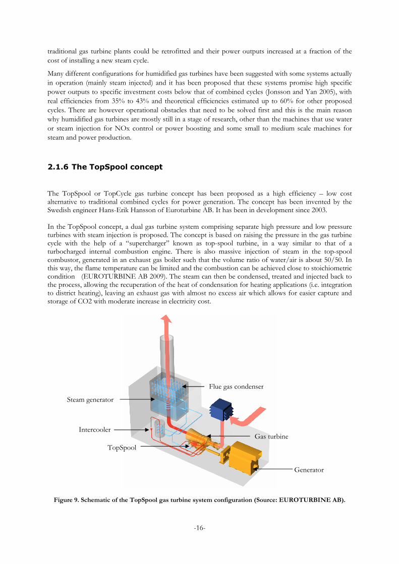
The TopSpool or TopCycle gas turbine concept has been proposed as a high efficiency – low cost alternative to traditional combined cycles for power generation. The concept has been invented by the Swedish engineer Hans-Erik Hansson of Euroturbine AB. It has been in development since 2003. In the TopSpool concept, a dual gas turbine system comprising separate high pressure and low pressure turbines with steam injection is proposed. The concept is based on raising the pressure in the gas turbine cycle with the help of a “supercharger” known as top-spool turbine, in a way similar to that of a turbocharged internal combustion engine. There is also massive injection of steam in the top-spool combustor, generated in an exhaust gas boiler such that the volume ratio of water/air is about 50/50. In this way, the flame temperature can be limited and the combustion can be achieved close to stoichiometric condition (EUROTURBINE AB 2009). The steam can then be condensed, treated and injected back to the process, allowing the recuperation of the heat of condensation for heating applications (i.e. integration to district heating), leaving an exhaust gas with almost no excess air which allows for easier capture and storage of CO2 with moderate increase in electricity cost.

Figure 9. Schematic of the TopSpool gas turbine system configuration (Source: EUROTURBINE AB).

Steam generator

TopSpool

Flue gas condenser

Intercooler Gas turbine

Generator

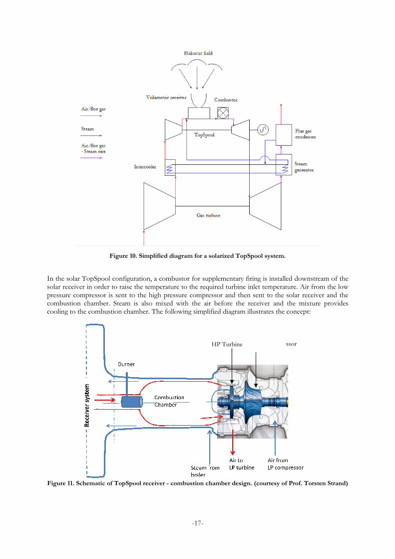
Figure 10. Simplified

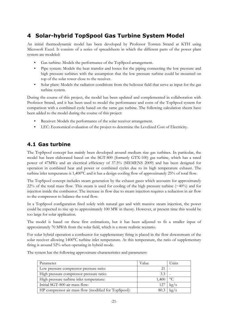
In the solar TopSpool configuration, a combsolar receiver in order to raise the temperature to the required turbine inlet temperature. Air from the low pressure compressor is sent to the combustion chamber. Steam is also mixed with the air before the receivercooling to the combustion chamber

Figure 11. Schematic of TopSpool receiver

-17-

. Simplified diagram for a solarized TopSpool system.

In the solar TopSpool configuration, a combustor for supplementary firing is installed downstream of the solar receiver in order to raise the temperature to the required turbine inlet temperature. Air from the low pressure compressor is sent to the high pressure compressor and then sent to the solacombustion chamber. Steam is also mixed with the air before the receiver and the mixture provides cooling to the combustion chamber. The following simplified diagram illustrates the concept:

ematic of TopSpool receiver - combustion chamber design. (courtesy of Prof. Torsten Strand)

HP Turbine HP Compressor

ustor for supplementary firing is installed downstream of the solar receiver in order to raise the temperature to the required turbine inlet temperature. Air from the low

and then sent to the solar receiver and the and the mixture provides

. The following simplified diagram illustrates the concept:

combustion chamber design. (courtesy of Prof. Torsten Strand)

HP Compressor

-18-

The TopSpool concept is expected to deliver efficiencies comparable to those of combined cycles, with the advantage that the high pressure turbine (the TopSpool) can be a highly compact and relatively economical unit, allowing for a variety of spatial configurations. In this regard, it has been proposed that the TopSpool could be integrated into a CSP gas turbine plant. For a conventional combined cycle plant it would be very difficult technically to install and operate the large scale gas turbine at the top of the tower. However for the TopSpool configuration, due to the small size of the TopSpool, it can be located either at ground level or on top of the tower next to the solar receiver while the large low pressure turbine can remain on the ground. This has been shown to be feasible by the SOLGATE project in which a helicopter engine was adapted and installed at the top of the tower next to the pressurized volumetric receiver.

-19-

3 Definition of operational scenarios and parameters

Because the main objective is to compare the technical and economic performance of the TopSpool cycle and a combined cycle under the same operation conditions, some simplifications have been made in order to reduce the complexity of the calculation:

Both cycles operate in the same undefined location, which allows for equal variable costs such as labor and fuel.

The evaluation is based on steady state operation for a certain number of hours/year defined by the solar conditions of the site. No transient, shut down and start up conditions are considered.

A fixed radiation flux on the solar field is defined for the selected location and the plants work based on this set flux and a number of solar hours per day. There are no hourly variations during the day and no daily or seasonal variations during the year. This would be more likely in tropical or sub tropical locations with low seasonal variations in day length, but in this case the same assumption is applied to a temperate climate region such as e.g. Spain.

No thermal storage is considered, which means that for operation during nighttime hours, e.g. for peak load hours during the evening, it operates solely on fuel power.

Definition of operation parameters:

The operation time has been defined according to the evaluation made by ECOSTAR, which states that the power conversion unit in a CSP system without storage runs about 1,800-2,500 full-load solar hours due to the limited sunshine hours (Pitz-Paal, Dersch and Milow 2005), depending mostly on location and seasonal variations. The ECOSTAR evaluation was made as described in section 4.5, i.e. full hybrid operation from 9 a.m. to 11 p.m.

A definition of 2,500 full solar load hours/year means about 7 hours/day of full sun power.

In a location like Seville, Spain, with an average normal direct irradiation of ca. 2,014 kWh/m2-year, this represents a constant irradiation value of approximately 0.8 kW/m2. The best solar locations near the Mediterranean can average up to 2,900 kWh/m2-year, which represents a constant irradiation value of approximately 1.1 kW/m2.

This is illustrated by the following figure:

Figure 12. Direct Normal Radiation potential for the Mediterranean Area in 2002 (kWh/m2-year, derived from satellite data). (Source: ECOSTAR)

-20-

Scenario number 1:

Operation in a region like northern Africa or the Middle East.

Solar flux = 1.0 kW/m2.

Solar availability: 2,500 full solar hours/year.

Plant availability: 4,905 hours/year, 9 a.m. to 11 p.m. including a capacity factor of 96% to account for forced and scheduled outages resulting in a capacity factor of 55%.

Scenario number 2:

Operation in a temperate region in southern Spain. This has been chosen given the availability of data from the SOLGATE report which allows also for comparison with other solar hybrid cycle evaluations.

Solar flux = 0.8 kW/m2.

Solar availability: 2,500 full solar hours/year.

Plant availability: 4,905 hours/year, 9 a.m. to 11 p.m. including a capacity factor of 96% to account for forced and scheduled outages resulting in a capacity factor of 55%.

Both scenarios represent an operation of 52% of time in hybrid mode and 48% in fuel only mode.

-21-

4 Solar-hybrid TopSpool Gas Turbine System Model

An initial thermodynamic model has been developed by Professor Torsten Strand at KTH using Microsoft Excel. It consists of a series of spreadsheets in which the different parts of the power plant system are modeled:

• Gas turbine: Models the performance of the TopSpool arrangement.

• Pipe system: Models the heat transfer and losses for the piping connecting the low pressure and high pressure turbines with the assumption that the low pressure turbine could be mounted on top of the solar tower close to the receiver.

• Solar plant: Models the radiation conditions from the heliostat field that serve as input for the gas turbine system.

During the course of this project, the model has been updated and complemented in collaboration with Professor Strand, and it has been used to model the performance and costs of the TopSpool system for comparison with a combined cycle based on the same gas turbine. The following calculation sheets have been added to the model during the course of this project:

• Receiver: Models the performance of the solar receiver arrangement.

• LEC: Economical evaluation of the project to determine the Levelized Cost of Electricity.

4.1 Gas turbine

The TopSpool concept has mainly been developed around medium size gas turbines. In particular, the model has been elaborated based on the SGT-800 (formerly GTX-100) gas turbine, which has a rated power of 47MWe and an electrical efficiency of 37.5% (SIEMENS 2009) and has been designed for operation in combined heat and power or combined cycles due to its high temperature exhaust. The turbine inlet temperature is 1,400°C and it has a design cooling flow of approximately 25% of total flow.

The TopSpool concept includes steam generation by the exhaust gases which accounts for approximately 22% of the total mass flow. This steam is used for cooling of the high pressure turbine (~40%) and for injection inside the combustor. The increase in flow due to steam injection requires a reduction in air flow to the compressor to balance the total flow.

In a TopSpool configuration fired solely with natural gas and with massive steam injection, the power could be expected to rise up to approximately 100 MW in theory. However, at present time this would be too large for solar application.

The model is based on these first estimations, but it has been adjusted to fit a smaller input of approximately 70 MWth from the solar field, which is a more realistic scenario.

For solar hybrid operation a combustor for supplementary firing is placed in the flow downstream of the solar receiver allowing 1400°C turbine inlet temperature. At this temperature, the ratio of supplementary firing is around 52% when operating in hybrid mode.

The system has the following approximate characteristics and parameters:

Parameter Value Units Low pressure compressor pressure ratio: 21 - High pressure compressor pressure ratio: 3.3 - High pressure turbine inlet temperature: 1,400 °C Initial SGT-800 air mass flow: 127 kg/s HP compressor air mass flow (modified for TopSpool): 80.3 kg/s

-22-

Total steam mass flow: 28.4 kg/s High Pressure turbine mixed flow: 110 kg/s Fuel flow (Natural gas): 1.7 kg/s Steam generator steam temperature(saturated at 70 bar): 283 °C LP Compressor efficiency 88 % LP Turbine cooling air flow 7 % IC Cooling power 15.3 MW High pressure compressor efficiency 80 % HP Turbine purge air flow 0.5 % Receiver exit temp 1000 °C Receiver pressure drop 1.0 % Receiver cooling air 1.0 % Reciver power ~74.9 MWth Combustor pressure drop 3.25 % Fuel heating value 48.6 MJ/kg Fuel compressor power 431 kW Combustor cooling air 0.5 % Fuel power ~81 MW

Table 1. Approximate operational parameters of TopSpool cycle.

Turbine parameter calculations, such as outlet temperature and pressure are done based on inlet and known engine parameters (such as compression ratio, isentropic efficiency) and according to the following equations: Temperature increase in the compressor:

�� − �� = ��� ∙ ������������ − 1� (4-1)

Where:

T1: inlet temperature

ηSC: isentropic efficiency of the compressor

KC: isentropic expansion coefficient for the fluid.

Temperature decrease in the turbine:

�� − �� = �� ∙ ��� �1 − ������������� � (4-2)

Where:

T3: inlet temperature

ηST: isentropic efficiency of the turbine

KT: isentropic expansion coefficient for the fluid.

Equipment power is calculated based on mass flow and enthalpy differences between defined points in the cycle, e.g. turbine or compressor inlet and outlet, steam generator inlet and outlet.

-23-

! = " ∙# $∆ℎ' = " ∙# (�$∆�' (4-3)

Where:

Qi: Equipment power.

m: Mass flow through equipment (compressor, turbine, heat exchanger).

∆h: Enthalpy difference between inlet and outlet.

Cp: Heat capacity of the fluid.

∆T: Temperature difference between inlet and outlet.

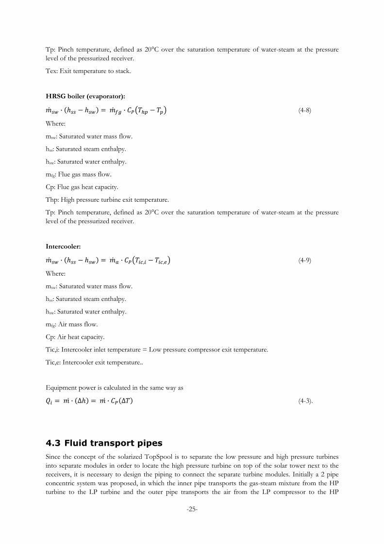
The following table illustrates the results of the model calculation for a generic simulation:

Solar heat input (MW) 74.9

Fuel heat input (MW) 81.1

LP Compressor power (MW) 39.8

LP turbine power (MW) 97.3

HP Compressor power (MW) 22.2

HP turbine power (MW) 47.5

Total turbine power (MW) 82.4

Gear box power (MW) 82.3

Generator power (MW) 79.5

El gross Efficiency % (fuel) 98

Net output power (MWel) 79.1

El net Efficiency % 50.7

Solar share (%) 25

Table 2. Simulation results of TopSpool cycle concept calculation.

Definition of efficiencies:

�)*,, = -.�/0 (4-4)

where:

ηel,f: Electrical gross efficiency (%).

Qf: Fuel heat input (MW)

Pel: Net output power (MWel)

�)* = -�/0 (4-5)

Where

ηel: Electrical net efficiency (%).

Q: Total heat input, fuel and solar (MW)

Pel: Net output power (MWel)

-24-

1�2 = -3- ∙ 454 (4-6)

Where

SSh: Solar share (%).

Qs: Solar heat input (MW)

th: Operating time in hybrid mode (Solar availability) (h/yr)

t: Total operating time (Plant availability) (h/yr)

4.2 Steam generator and intercooler

The TopSpool concept is based on the injection of steam into the dual gas turbine system. The idea being that the added mass flow and heat capacity of the steam will significantly increase the power output of the gas turbines leading to a higher overall efficiency comparable with that of a combined cycle but without the need of incurring in high investment costs related to the Rankine cycle equipment.

A configuration is proposed in which the steam is generated in two pieces of equipment: A heat recovery steam generator –HRSG– similar to those used in combined cycles but with the advantage that the heating media is a mixture of flue gases and steam, which similarly to what occurs with the rest of the cycle, provides for better heat transfer characteristics when compared to flue gas only (i.e. flue gas in which the only steam content is that generated from combustion), thus it can be predicted that this piece of equipment can be comparatively smaller and cheaper. Also in the TopSpool cycle the steam generated by the HRSG only needs to be saturated or slightly superheated because the rest of the superheating can be done inside the solar receiver and combustion chamber. Given its low temperature, part of this steam can be used as an effective cooling medium in the combustion chamber.

The second steam generating equipment is the intercooler. In this case, a common intercooler system generates steam using the air coming from the low pressure compressor while at the same time it helps in maintaining a good performance on the high pressure compressor. The intercooler is fed with saturated water from the HRSG and provides the extra heat needed to generate saturated steam.

The steam from the HRSG and intercooler are collected in a single pipe which leads to the pressurized volumetric receiver, as can be seen in Figure 10. From this point, the air and steam are heated up to a temperature near 1,000°C by the solar receiver, enter the combustor in which the temperature is increased up to the turbine inlet temperature ~1,400°C, and then the mix is expanded through the turbines. After expansion the mix goes through the steam generator and from there to a condenser in which steam is recovered to be fed back into the HRSG and intercooler.

The calculation for the HRSG and intercooler is based on the mass and energy balance for the flue gas, low pressure compressed air, and steam:

HRSG pre-heater (economizer):

"# ,6 ∙ 7ℎ86 − ℎ,69 = "# ,: ∙ (�7�; − �)<9 (4-7)

Where:

mfw: Feed water mass flow.

hsw: Saturated water enthalpy.

hfw: Feed water enthalpy.

mfg: Flue gas mass flow.

Cp: Flue gas heat capacity.

-25-

Tp: Pinch temperature, defined as 20°C over the saturation temperature of water-steam at the pressure level of the pressurized receiver.

Tex: Exit temperature to stack.

HRSG boiler (evaporator):

"# 86 ∙ $ℎ88 − ℎ86' = "# ,: ∙ (�7�2; − �;9 (4-8)

Where:

msw: Saturated water mass flow.

hss: Saturated steam enthalpy.

hsw: Saturated water enthalpy.

mfg: Flue gas mass flow.

Cp: Flue gas heat capacity.

Thp: High pressure turbine exit temperature.

Tp: Pinch temperature, defined as 20°C over the saturation temperature of water-steam at the pressure level of the pressurized receiver.

Intercooler:

"# 86 ∙ $ℎ88 − ℎ86' = "# = ∙ (�7�!>,! − �!>,)9 (4-9)

Where:

msw: Saturated water mass flow.

hss: Saturated steam enthalpy.

hsw: Saturated water enthalpy.

mfg: Air mass flow.

Cp: Air heat capacity.

Tic,i: Intercooler inlet temperature = Low pressure compressor exit temperature.

Tic,e: Intercooler exit temperature..

Equipment power is calculated in the same way as

! = " ∙# $∆ℎ' = " ∙# (�$∆�' (4-3).

4.3 Fluid transport pipes

Since the concept of the solarized TopSpool is to separate the low pressure and high pressure turbines into separate modules in order to locate the high pressure turbine on top of the solar tower next to the receivers, it is necessary to design the piping to connect the separate turbine modules. Initially a 2 pipe concentric system was proposed, in which the inner pipe transports the gas-steam mixture from the HP turbine to the LP turbine and the outer pipe transports the air from the LP compressor to the HP

-26-

compressor and also provides cooling for the inner pipe in which the wall temperatures are close to 900°C due to the high temperature flow from the high pressure turbine.

A third pipe is also needed to transport the steam from the HRSG to the receiver.

The modeled inner pipe material was evaluated as steel with ceramic coating acting as a thermal barrier on both sides, the modeled outer pipe as metal with exterior insulation.

Heat transfer calculations were made involving convective and conductive heat transfer across the pipe walls using the following heat transfer dimensionless parameters: the Reynolds number, Prandtl number and Nusselt number. The overall heat transfer coefficient was calculated and used to calculate the heat transfer between the hot and cold pipe:

?@ = A∙<B = C ∙ D ∙ EF (4-10)

Where Re: Reynolds number.

u: fluid velocity.

x: characteristic length, in this case the diameter of the tube.

v: the kinematic viscosity of the fluid.

The kinematic viscosity can also be calculated as the dynamic viscosity µ divided by the density of the fluid ρ.

GH = (� ∙ FI (4-11)

Where:

Pr: Prandtl number.

Cp: specific heat.

µ: dynamic viscosity.

k: thermal conductivity of the fluid.

JC = 2∙<I (4-12)

Where:

Nu: Nusselt number.

h: convective heat transfer coefficient.

x: characteristic length.

k: thermal conductivity for the fluid.

The above equation is used to calculate h, the heat transfer coefficient, using a determined value of Nu.

The Nusselt number is evaluated using the Dittus-Boelter equation for fully developed turbulent flow in tubes:

JC = 0.023 ∙ ?@O.P ∙ GHQ (4-13)

-27-

Where:

Nu is the Nusselt number

Re is the Reynolds number

Pr is the Prandtl number

n = 0.3 for cooling of the fluid.

Then the overall heat transfer coefficient was calculated using the convective heat transfer coefficient for the fluids, the thermal conductivity of the pipe materials and their thickness:

�R = �2� + TI + �2� (4-14)

Where:

U: overall heat transfer coefficient,

hi: convective heat transfer coefficient for the fluid

δ: wall thickness

k: wall thermal conductivity.

After calculation the design was changed to separate parallel pipes for the different fluids, due to the amount of heat loss from the inner pipe. This is explained and discussed in the results section (section 7.3).

4.4 Solar receiver

The solar receiver module models the heat transfer in the pressurized receivers. This is of particular importance because so far pressurized receivers have been used to heat air only. Since the TopSpool system uses a mixture of air and steam at high pressure as working medium (before the combustor), it is expected that similarly designed receivers can operate at higher concentration ratios leading to higher receiver power due to the increased heat capacity and density of the working medium. In other words, due to the higher heat capacity of the air-steam mixture compared to air, a similar receiver would be able to operate at higher load, effectively heating a considerably higher mass flow and providing greater power.

According to the literature, multiple receivers can be placed at the focal point on the tower and connected in parallel and in series to raise the temperature gradually. The receiver calculation has been made based on multiple receivers with an individual aperture area of 1.24 m2, which have been built and tested in the SOLGATE project. In this manner, a cluster of low temperature receivers would be installed on the outer perimeter of the focal point where irradiation may be more scattered and less intense, then medium and high temperature receivers would be located progressively closer to the center of the focal point where the irradiation is most intense.

A thorough design for a receiver is in itself a very complex task and goes beyond the scope of this work. The approach for a preliminary receiver design has been more focused on obtaining reasonable values for the number, area and ultimately cost of receivers in order to be able to integrate this part of the system into the economic evaluation.

It is also important to note that pressurized receivers reported by the SOLGATE project have operated with pressure levels of approximately 6.5 Bar. The shift from atmospheric to pressurized receiver designs has required the use of pressure resistant domed quartz windows like the one shown in Figure 2.

Even though the pressure level of the TopSpool concept is much higher, in the order of 60 Bar, it is assumed here for simplicity that a similar type of window can be designed to operate at such pressure

-28-

conditions, or that the same total aperture receiver area can be covered by installing a greater number of smaller receivers in which the window diameters are small enough to be able to withstand the flow pressure.

It should be noted that the temperature levels achieved in the receiver window are also of concern due to the increased solar concentration ratios that come as a consequence of the reduced receiver area. With the help of the Explore Solar group at KTH, some preliminary calculations have been performed to assess how the increased pressure and concentration ratios would affect the receiver and window, coming to a first conclusion that the temperature of the window could reach levels of up to 1,500°C because the absorptivity is constant, so additional cooling methods would be required to preserve its integrity.

In any case, it is assumed here that future receiver designs, either pressurized volumetric receivers or advanced design and material tubular receivers will be able to withstand high concentration ratios and reach fluid temperatures higher than 1,000°C. In fact, receivers have been developed by CONSOLAR in Israel which have produced air temperatures of 1300°C.

The approach for the preliminary receiver design was to calculate a flow number or flow area, based on the reported values of pressure, temperature and mass flow of pressurized air receivers:

U = V# √X�� (4-15)

Where: K: flow area number.

m: mass flow through the receiver.

R: Specific gas constant.

T: Inlet temperature.

P: Fluid pressure.

The flow number gives an idea of the performance of a particular receiver and serves to evaluate the mass flow that could be sent to the receiver under different fluid conditions, in this case the air/steam mixture with higher gas constant and pressure values.

Using the mass flow for the air-steam mixture, the determination of the number of necessary receivers connected in parallel is done by dividing the total mass flow of the system by the calculated mass flow for each receiver.

Y = V# 3Z3[/\V# ]/^/_`/] (4-16)

where:

n: number of parallel receivers

msystem: total mass flow going through the receiver cluster.

mreceiver: calculated mass flow for each receiver.

The values used to calculate the flow number for the pressurized air receiver are those reported by Heller (Heller, et al. 2006) for the design, construction and evaluation of the pressurized air receiver used in the SOLGATE project in Spain.

The following table illustrates the values used to calculate the flow number for the different types of air receivers (i.e. low, medium and high temperature modules) and the number of necessary receivers for the flow conditions of the TopSpool cycle:

-29-

Solgate receiver Test 1 Units LT MT HT m 1.357 1.357 1.357 kg/s T 569 766 880 K P 650.0 650.0 650.0 kPa Q 279 169 276 kWth cp air 1.044 1.091 1.117 kJ/kgK K (Flow number) 843.8 979.0 1049.4 m2

Solgate receiver Test 2 LT MT HT m 1.327 1.327 1.327 kg/s T 563 689 886 K P 650.0 650.0 650.0 kPa Q 174 280 217 kWth cp air 1.043 1.072 1.118 kJ/kgK K (Flow number) 820.8 908.0 1029.7 m2

TopSpool receiver LT MT HT m 10.733 11.036 11.205 kg/s T 742 902 1062 K P 6337.9 6337.9 6337.9 kPa Q 2,388 2,471 2,570 kWth/receiver cp mix 1.390 1.400 1.433 kJ/kgK K (Flow number) 832.3 943.5 1039.5 n 9 9 9 Receivers Q 21,846 22,612 23,510 kWth/cluster Q 67,968 kWth total Table 3. Calculation results for preliminary pressurized solar receiver design.

In theory, as the heat transfer characteristics of the fluid improve, the number of receivers that would be needed to supply the necessary heat for the desired temperature gains decreases. Nevertheless, the concentration ratio of the solar plant acts as a barrier setting an upper limit for the number of receivers, i.e. there has to be a minimum receiver area so that the concentration ratio is close to 2000 for which temperatures of 1000°C have been demonstrated, but not so much higher that it represents a thermal flux that the receiver might not be able to withstand.

Here, the concentration ratio is defined as

( = a3.a] (4-17)

Where:

C is the concentration ratio.

Asf is the total heliostat required area (m2).

Ar is the receiver area.

In this case, the required solar power is in the order of 70 MWth, which for an incident radiation value of 1 kW/m2 requires a solar field area of approximately 0.13 km2. For a concentration ratio of ~2500, the minimum receiver area is then set to about 68 m2, or 57 receivers with a unit area of 1.24 m2.

-30-

4.5 Solar field

The third module models the solar field data in order to produce the inputs for the gas turbine system. Values have been extracted from the literature, mainly from NREL and the SOLGATE project, and adjusted to the system requirements.

The heliostat field required area and the number of required heliostats is calculated based on the following equations:

b8, = G ∙ �8, ∙ c (4-18)

Where:

Asf is the total heliostat required area (m2).

P is the required solar power from the solar field (kW), determined by the power cycle calculation given a receiver outlet temperature of 1,000°C.

ηsf is the annual efficiency of the solar field.

I is the incident direct beam irradiation (kW/m2).

J = a3.a5 (4-19)

Where:

N is the number of heliostats

Ah is the defined area of each heliostat.

Solar field annual efficiency: The efficiency of the solar field is defined by a number of constraints, such as mirror reflectivity and cleanliness, light dispersion due to atmospheric dust and pollutants and wind, tracking precision, field geometry and location in relation to the tower, availability, shadowing effects by tower and other heliostats, among others. Calculated and/or reported efficiencies range from ~50% (NREL 2003) (Schwarzbözl, et al. 2006) up to 70% in theory (Spelling 2009).

The following table illustrates an example of annual solar collection efficiency for the Solar Tres power plant in U.S.:

Table 4. Annual heliostat field efficiency. (NREL 2003)

An efficiency value of 55% is chosen based on actual data reported from the literature. This value is further adjusted by the receiver efficiency. SOLGATE reports receiver efficiency values of 78+-4%.

-31-

NREL projects receiver efficiencies of up to 83.5% in the long term. A receiver efficiency of 80% is used in the calculation.

Ground beam irradiation: Solar concentration systems can only use direct beam irradiation, thus this value must be chosen taking into account that diffuse radiation does not contribute to the power production of these systems.

For simplicity, and because the idea is to compare the TopSpool cycle with a combined cycle (not to evaluate a location of the plant), no site-specific data for hourly radiation has been obtained.

Two values for evaluation have been chosen: 0.8 kW/m2 and 1.0 kW/m2. The operational time has been defined as per the reported values in ECOSTAR: free-load operation or hybrid operation, 100% load between 9:00 a.m. and 11 p.m. every day, average availability of 96% to account for forced and scheduled outages resulting in a capacity factor of 55% (Pitz-Paal, Dersch and Milow 2005).

Heliostat area: NREL reports values from 48 up to 148 m2. SOLGATE reports values of 121 m2. It is assumed here that the heliostats are slightly curved and can provide a concentration ratio of up to 20, thus it is not necessary to limit the size of the heliostats according to the area of the receiver.

Tower height:

The calculation for the tower height is based on the following empirical formula, calculated from the values reported by SOLGATE:

d4e6)f = 0.52 ∙ hb8, (4-20)

Where:

Htower: is the tower height (m).

Asf: is the area of the solar field (m2)

-32-

5 Solar hybrid combined cycle

A model for a solar hybrid combined cycle has been used for comparison with the TopSpool concept. It has already been mentioned that the TopSpool is expected to deliver similar electrical efficiency compared to a combined cycle thanks to the injection of steam inside the gas turbine, but at an overall lower cost because of the lower investment and operational costs which are expected from a more compact power plant.

Figure 13. Solarized gas turbine plant schematic: combined Brayton and Rankine cycle (Schwarzbözl, et al. 2006).

The solar hybrid combined cycle model has been developed by professor Strand using Excel based on the SGT-800, and it has been adapted to match the operational conditions of the TopSpool model. In this regard, the power plant components are calculated in the same way as the TopSpool, e.g. the solar field, tower, fuel system, etc.

The main differences between the combined cycle plant and the TopSpool plant are:

Piping: Only two pipes, transporting the air from the compressor to the receiver, then from the receiver to the combustor of the gas turbine are needed in the tower of the combined cycle plant. In the TopSpool plant, one pipe transports the air from the LP compressor to the receiver, another transports the gas-steam mixture from the HP turbine to the LP turbine and one more transports the steam from the HRSG to the receiver, for a total of three. Similarly to the TopSpool case, the material and size of these elements creates a constraint on the temperature level that they can withstand, which in practical terms means that the receiver exit temperature has to be limited to ~900-920°C and this in turn represents a limit on the amount of solar heat input.

Solar receiver: For the combined cycle plant the Brayton cycle would operate on gas only as working medium. After combustion and expansion in the gas turbine the exhaust gas goes to the heat recovery steam generator to generate steam for the Rankine cycle.

In the combined cycle, the gas turbine operation is similar to the low pressure turbine of the TopSpool system (they are both modeled based on the operational conditions of the SGT-800). The pressure ratio is approximately 20, with the pressure after the compressor being in a level around 20 Bar. This affects the

-33-

calculation of the receiver in the same manner as for the TopSpool: The increased mass flow and pressure, when compared to the reported values of pressurized volumetric receivers is expected to improve the heat transfer characteristics of the receiver allowing for higher power and lower required receiver area. However, in the combined cycle case, the gas turbine has a cooling requirement of approximately 25% of the air mass flow, which means than in this case less air actually goes through the receiver.

The calculation for the receiver of the solar combined cycle has been performed using the same equations for the calculation of the flow number and mass flow as section 4.4, based on a receiver outlet temperature of 920°C as explained in the pipe description.

Solar field: The receiver power required determines the size of the solar field. The conditions and equations are the same as section 4.5, matching the values for direct normal irradiation, solar field efficiency, heliostat area. The lower receiver temperature and solar input described above result in a smaller solar field for the combined cycle when compared to the TopSpool case, but this also means that the combined cycle has a lower overall solar share, as is shown in section 7.

Steam generator: This is expected to be a bigger unit for the combined cycle because superheating is desirable to maximize cycle efficiency and to avoid erosion in the steam turbine. Having no steam turbine, the TopSpool plant can generate saturated or barely superheated steam which is further heated in the receiver and combustor, allowing for a smaller package of steam generator and condenser.

The steam mass flow is somewhat lower for the combined cycle with ~18kg/s for the steam turbine compared to 28kg/s for the TopSpool system. This is explained by the need to use steam for cooling of the combustor and turbines in the TopSpool system.

Turbines: Obviously, the combined cycle needs a steam turbine for the Rankine cycle part of the system. The TopSpool is composed of two separate gas turbines, high and low pressure respectively, whereas the combined cycle is composed of a gas turbine and a steam turbine. Because of the high volumetric expansion of steam, the steam turbine is a massive and costly piece of equipment, which in the TopSpool system is replaced by another gas turbine.

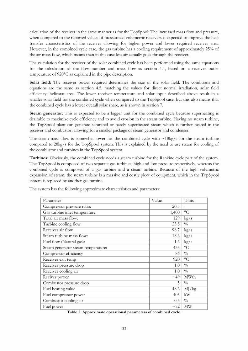
The system has the following approximate characteristics and parameters:

Parameter Value Units Compressor pressure ratio: 20.5 - Gas turbine inlet temperature: 1,400 °C Total air mass flow: 129 kg/s Turbine cooling flow 23.5 % Receiver air flow 98.7 kg/s Steam turbine mass flow: 18.6 kg/s Fuel flow (Natural gas): 1.6 kg/s Steam generator steam temperature: 435 °C Compressor efficiency 86 % Receiver exit temp 920 °C Receiver pressure drop 1.0 % Receiver cooling air 1.0 % Reciver power ~49 MWth Combustor pressure drop 5 % Fuel heating value 48.6 MJ/kg Fuel compressor power 405 kW Combustor cooling air 0.5 % Fuel power ~72 MW

Table 5. Approximate operational parameters of combined cycle.

-34-

6 Economic model

In addition to the evaluation of technical performance for the TopSpool concept against competing technologies, an economic evaluation was also realized to compare the concept potential to deliver similar capacity and efficiency at lower overall cost.

It has been mentioned before that one of the main advantages of the TopSpool concept is the possibility to eliminate the steam turbine by steam injection into the gas turbine, creating a more compact version of a combined cycle. It is generally accepted that the bottom cycle usually accounts for up to 2/3 of the investment cost of a combined cycle but only provides about 1/3 of the power. In the TopSpool concept the steam turbine is effectively replaced by the steam injected gas turbine, resulting in a more compact unit.

Even though the steam generator or boiler cannot be eliminated, it can be simplified and reduced in size by designing it to provide saturated or slightly superheated steam, leaving the rest of the superheating to the gas turbine combustor, thus also reducing the cost for this piece of equipment. Having less equipment usually means also lower maintenance costs.

One of the main challenges comes from the fact that the TopSpool is a concept in development, so no actual power plants have been built using this cycle, either for fossil fuel based or hybrid operation. There are reference values for solar combined cycle plants, however the changes necessary to operate with steam injection and increased pressure ratios have to be taken into account and rely on estimations.

Another challenge arises from the size of the solar tower and receiver. To date, no power plants of medium to large scale have been constructed using solarized gas turbines. Estimations can be based on the reported cost of receivers for small scale plants and tests or other theoretical studies (e.g. from SOLGATE or NREL), however a direct extrapolation might underestimate the effect of possible economies of scale from mass manufacturing of receivers or manufacturing of larger ones.

The economic indicators commonly used for evaluation of power generation are Net Present Value - NPV (as in most investment projects of any kind) and Levelized Cost of Electricity – LEC which represents the cost of production per energy unit (US$ or € per kWh) taking into consideration capital and operational costs.

NPV is an indicator used to determine the economic viability of a project, i.e. whether it makes sense as an investment. The NPV of the project should be positive after a number of years in which the project is expected to break even (i.e. cover the cost of initial investment, operation and maintenance, and debt), thus providing net income for the rest of the duration of its operational lifetime. This is determined by a number of parameters, such as the interest rate for debt, debt-equity ratio, expected return on equity, taxation levels, inflation, etc.

The levelized cost of electricity is the minimum price at which the project generated electricity must be sold to achieve a neutral or positive NPV after a determined number of years, in other words, it is the price at which the electricity must be generated to make the project financially viable.

ij( = ∑ a[lm&o[p[q�∑ r[p[q� (6-1)

Where:

• LEC = Average lifetime levelized electricity generation cost • At= Annuity payment for capital investments for the year t. • O&Mt = Yearly operation and maintenance costs, including staff, fuel, spares, etc.

-35-

• Et = Electricity generation in the year t • n = Life of the system (years)

6.1 Definition of economic scenarios

For the evaluation of the TopSpool project, two separate investment scenarios have been evaluated, with the following conditions defined for the economic parameters:

6.1.1 Investment conditions as defined by SOLGATE.

Within this scenario, the following conditions for the annuities calculation and cost escalation are defined:

General inflation rate: 2.5%

Debt-equity ratio 75%-25%

Debt interest rate: 4.2%

Equity interest rate (expected return on equity): 14%

Weighted average cost of capital WACC (based on debt-equity ratio): 7.25%

Debt payback and investment recovery time: 12 years.

Operational lifetime: 20 years.

These values are similar to those utilized by Schwarzbözl et.al. for the evaluation of other solar gas turbine and combined cycle systems. They have been chosen as a reference because this is deemed to be a realistic economic investment evaluation, i.e. the type that would actually be made by an electricity company to evaluate the investment.

Depreciation is assumed linear during the lifetime of the plant.

Depreciation = Investment/n.

The annuity plan is structured based on equal yearly payments, i.e. interest + amortization = constant, in which interest is higher at the beginning of the payment period and lower at the end.

6.1.2 Investment conditions as defined by ECOSTAR.

The ECOSTAR project has evaluated several solar thermal power generation technologies and compared their potential LEC based on the following conditions:

Interest rate (kd): 8%

Depreciation and payback time (n): 30 years.

The levelized electricity cost has been evaluated by ECOSTAR using the following simplified formula suggested by the IEA (International Energy Agency 1991):

with

-36-

6.2 TopSpool cycle Investment costs

The investment costs have been defined for the most important pieces of equipment. It is assumed in most cases that the cost of equipment correspond to commercially available and mature technology, so there is no special consideration for costs of development engineering, and that the equipment can be mass produced.

Solar field:

The cost of the solar field depends on the number of heliostats needed to supply the required power and their size. Cost figures are obtained in €/m2 of heliostat area.

Schwarzbözl et.al. have reported a cost of 132 €/m2 for the year 2003. Since then there has been some deployment of solar fields in various countries around the world, so this value is considered to be relatively high for the year 2011.

SANDIA has published a report with calculated heliostat costs and proposed cost reduction strategies for the year 2006. According to this report, heliostat costs of US$ 100 are desirable to achieve enough cost reductions for competitive levelized costs of electricity, which they have evaluated to be possible in the medium term via research and development technology improvements, cost reductions due to higher economies of scale in mass production and a natural learning curve during the development of several GW of installed power over a decade or more. They have evaluated two different heliostat technologies, namely glass-metal square heliostats and stretched membrane round heliostats. They report that even though the unit cost/m2 of the stretched membrane heliostat is higher, there are advantages like the possibility of tighter packing of the heliostats in the field leading to a higher solar field efficiency.

According to SANDIA the major aspect that will influence cost reduction of heliostats is the volume of production. Even though they report an optimum heliostat area of approximately 150 m2, it is suggested that optimum costs can be achieved with areas as low as 50 m2. For this reason the concern of a higher cost of heliostats based on a limited area to the size of the solar receiver is dismissed, given that 121m2 is a reasonable heliostat size for the TopSpool configuration.

The prices reported by SANDIA for the glass metal heliostat range from US$164/m2 (~112€/m2) for a production rate of 5,000 units/year and US$126/m2 (~86€/m2) for 50,000 units/year (SANDIA 2007). For the stretched membrane heliostats the price ranges between US$130/m2 (~89€/m2) and US$170/m2 (~116€/m2).

According to the reviewed literature a future market price of ca. 100€/m2 or lower is deemed reasonable for the evaluation.

Receiver:

As described in section 2.1.3, there are two types of secondary receivers: a tubular or spiral receiver for low temperature ranges, and pressurized volumetric receivers for the medium and high temperature ranges. Similarly to the solar field, the cost figures for the receivers are specified per unit area.

Schwarzbözl et.al report values of 16,000 €/m2 for the low temperature receiver, 33,000 €/m2 for the medium temperature receiver and 37,000 €/m2 for the high temperature receiver clusters. This is one of the items which is still under development and research, thus it is difficult to estimate price reductions for a mature technology. Also, the receiver for the TopSpool concept should operate at much higher pressure and heat flux conditions than those designed so far for solar gas turbines. For this reason, the investment costs for the receiver are left unmodified at the values reported for the SOLGATE project.

Conventional power plant:

The conventional power plant consists of the power block, fuel system, cooling system, condenser, generator, grid connection and other auxiliary equipment.

-37-

NREL has reported values for the capital cost of solar plants based on power tower with storage technology and evaluated the cost reduction potential in the medium and long term (NREL 2003). They have reported values for the electrical power block (which includes steam turbine and generator, steam turbine and generator auxiliaries, feed water and condensate systems) of up to US$400/kWe, and values for other auxiliaries or “balance of plant” (which include condenser and cooling tower system, water treatment system, fire protection, piping, compressed air systems, closed cooling water system, instrumentation, electrical equipment, and cranes and hoists) of up to US$400/kWe for a plant scale of 50 MWe, which amounts to a total of around US$800/kWe (~550 €/kWe) for the whole “conventional power plant”, which accounts for the gas and steam turbines.

For the TopSpool, the cost has been defined as 300 €/kWe installed for both turbines. This is deemed to be a reasonably representative price of commercial gas turbine power plants of medium scale.

Piping:

The pipes that transport the working media between turbines have been estimated apart from the conventional power plant because in a regular plant the low and high pressure turbines would be a single unit or at least would be located in close proximity. For the estimation, the cost of metal and insulation has been considered. The cost of metal is assumed as 4 €/kg for stainless steel, either high temperature alloy such as 253 MA or 353 MA or medium temperature alloy such as nickel alloy. Insulation is assumed to be mineral wool blankets with a price of 5 €/kg.

Steam generator and condenser:

The steam generator for the TopSpool cycle differs from conventional combined cycle steam generators in the following aspects: First, the design has been proposed so that there is no requirement for superheating from the steam generator, thus avoiding the need of the superheater which would be expected to be the most expensive part of the heat exchanger because of its temperature conditions. Second, the steam generator can remain simple by using only one pressure level, which also limits the cost when compared to multiple pressure HRSG units. This makes it difficult to estimate the cost of the steam generator based on reported values because any figure must be scaled down to account for the simplified arrangement from conventional units which often operate at multiple pressure systems including superheating and reheating.

Zhao et al. report values for 1, 2 and 3 pressure levels HRSG systems for a combined cycle power plant (Zhao, et al. 2003). For the single pressure system, values have been calculated using their reported data and range from 23.6 to 26 US$kW (~17 €/kW) of total net power (gas+steam).

For the calculation of the TopSpool cycle, a value of €11/kW is used, assuming that the absence of the superheater reduces the cost of the equipment by 1/3.

Tower:

In the evaluation made by SOLGATE the tower is considered to be a made of concrete for the combined cycle plant. They report a value of 1,682,000 € for a tower of 130 m for the largest system evaluated, i.e. a solar combined cycle. A simple extrapolation for a 150 m tower results in an approximate value of €1,940,000 for the cost of the tower.

For the TopSpool concept it is proposed that the low pressure turbine remains at ground level, thus only the small high pressure turbine and related generation equipment such as gearbox and generator need to be installed on top of the tower. A wind turbine type of tower has been evaluated to assess its viability as solar tower. It is well known that wind turbine towers are installed with heights comparable to the height of the TopSpool theoretical plant (up to 150 m) and the fact that wind turbine towers are being mass produced allows for the expectation that it will be cheaper when compared to a custom built tower.

The main concern has been the weight of the equipment to be installed on top of the tower, i.e. the receiver, high pressure gas turbine, gearbox, generator and auxiliary equipment. It is expected that the

-38-

heaviest equipment are the gearbox and generator, thus it has been necessary to determine an approximate weight for these. An ABB generator with an output of ~26,000 kVA was found that weighs approximately 95 tons. This would be somewhat similar to the expected power produced by the high pressure turbine of approximately 23 MW.

Reported values for wind turbine hub and nacelle weights have been gathered to compare with the expected weight of the solar equipment.

The Siemens SWT 3.6 MW rotor and nacelle have a combined weight of approximately 225,000 kg and are mounted on a 90 m tubular steel tower.

The theoretical NREL 5 MW wind turbine, designed as a large wind turbine that is representative of typical utility-scale land- and sea-based multi-megawatt turbines (Jonkman, et al. 2009), has a rotor weight of 110 tons and a nacelle weight of 240 tons for a total top weight of 350 tons. This turbine and a 3 MW turbine scaled down from it have been evaluated in a report elaborated by ELFORSK for Vindkraftverk on 2010 (Engström, et al. 2010). The 3 MW wind turbine has a rotor weight of 56.5 tons and a nacelle weight of 120 tons, for a combined weight of 176.5 tons.

The report evaluates different types of towers, e.g. steel welded, steel with friction joints, concrete, concrete-steel hybrid, lattice, and wood, in terms of structural characteristics and cost. Lattice and wood are not considered for the TopSpool concept because the tower is also expected to provide housing for the piping that connects the high pressure and low pressure turbines.

According to the report, welded steel towers face structural problems for heights higher than 150 m for the 3 MW turbine and 100 m for the 5 MW turbine, because of limitations on the maximum base diameter and plate thickness. However, steel with friction joints, concrete and concrete-steel, can be used for hub heights of up to 175 m.

The following table illustrates the reported costs for the 5 MW wind turbine 150 m tower for these materials.

Tower material Cost

Steel with friction joints. €1,942,000

Concrete €2,115,000

Concrete-steel hybrid €1,824,000

These values are similar to the value reported by SOLGATE for the concrete tower of €1,940,000, although in that case the concrete tower would compare with the steel with friction joints tower reported by ELFORSK. They also report that hybrid towers are widely used by wind turbine manufacturer Enercon, which makes one of the largest wind turbines in the world today at 7.5 MW, and also by tower manufacturer Advanced Tower Systems.

The value for the concrete-steel hybrid has been chosen as reference and extrapolated to fit the TopSpool tower height.

6.2.1 Summary of TopSpool cycle investment costs.

Investment Unit cost Units Total cost % of Investment Solar field 100 €/m2 € 17,242,500 35.9% LT receiver 16,000 €/m2 € 367,119 0.8% MT receiver 33,000 €/m2 € 757,183 1.6%

HT Receiver 37,500 €/m2 € 860,435 1.8%

-39-

HP turbine block 300 €/kW € 7,651,189 15.9% LP turbine block 300 €/kW € 17,328,972 36.0% Piping 4 €/kg € 253,974 0.5%

Pipe insulation 5 €/kg € 45,585 0.1%

Steam generator 11 €/kWe € 875,173 1.8%

Intercooler 4 €/kWth € 61,496 0.1%

Tower 12,160 €/m € 2,625,651 5.5%

Total cost € 48,069,277 Table 6. Summary of TopSpool power plant investment cost for the 1kW/m2 irradiation case.

Figure 14. Summary of TopSpool power plant investment cost for the 1kW/m2 irradiation case.

Investment Unit cost Units Total cost % of Investment Solar field 100 €/m2 € 21,598,500 40.5% LT receiver 16,000 €/m2 € 463,729 0.9% MT receiver 33,000 €/m2 € 956,442 1.8%

HT Receiver 37,500 €/m2 € 1,086,865 2.0% HP turbine block 300 €/kW € 7,653,813 14.4% LP turbine block 300 €/kW € 17,330,497 32.5% Piping 4 €/kg € 284,250 0.5%

Pipe insulation 5 €/kg € 51,019 0.1%

Steam generator 11 €/kWe € 875,319 1.6%

Intercooler 4 €/kWth € 61,497 0.1%

Tower 12,160 €/m € 2,938,656 5.5%

Total cost € 53,300,587

Table 7. Summary of TopSpool power plant investment cost for the 0.8kW/m2 irradiation case.

35.9%

0.8%

1.6%

1.8%

15.9%

36.0%

0.5%

0.1% 1.8%0.1%

5.5%

Solar field

LT receiver

MT receiver

HT Receiver

HP turbine block

LP turbine block

Piping

Pipe insulation

Steam generator

Intercooler

Tower

-40-

Figure 15. Summary of TopSpool power plant investment cost for the 0.8kW/m2 irradiation case.

6.3 TopSpool cycle Operational costs

Operational costs can vary considerably depending on location, degree of automation, fuel cost, labor, among others. Moreover, operational costs vary from plant to plant and this kind of commercial data is generally treated as confidential by companies, thus it is usually very difficult to obtain.

Because no TopSpool cycles have ever been built and operated, even for fuel only configurations, there is no available real data upon which to rely.

6.3.1 Operation and maintenance

Schwarzbözl et.al. report O&M costs based on first and second generation power plants, i.e. first of kind and successfully implemented technology respectively, for their 16MW combined cycle:

1st gen (k€/y*MW) 2nd gen (k€/y*MW)

150.2 121.2 Table 8. SOLGATE operation and maintenance costs for first and second generation solar combined cycle

(EUROPEAN COMMISSION - Directorate-General for Research. 2005)

Data has also been reported by NREL on solar technology cost forecasts (NREL 2003) for solar tower technology. However, the report focuses solely on solar only steam generation with thermal storage from power towers. Estimates vary from US$0.033/kWhe for 2004, US$0.008/kWhe for 2008 and US$0.006/kWhe for 2020.

Values of operation and maintenance costs based on installed capacity (k€/y*MW) are preferred over costs based on electricity production ((€/kWh) because the latter are determined by the operation conditions of the plant, hence they represent a-posteriori results of actual operation and/or simulation rather than initial conditions based on expected fixed and variable costs.

A value of 121 k€/y*MW is applied for the calculation of the TopSpool cycle to be consistent with the assumption that the plant will operate under mature technology and market spread conditions.

40.9%

0.7%

1.4%1.6%

14.5%

32.8%

0.5%0.1%

1.7%0.1%

5.6%

Solar field

LT receiver

MT receiver

HT Receiver

HP turbine block

LP turbine block

Piping

Pipe insulation

Steam generator

Intercooler

Tower

-41-

6.3.2 Fuel

Natural gas prices vary greatly depending on location, consumption and other factors. A fixed price for natural gas has been obtained from Europe’s Energy Portal (www.energy.eu) for January 2011 for industrial consumers. The webpage summarizes prices for all EU countries and gives data for small and large industrial consumers. A sample of the data available on the webpage is shown in the following figure:

Figure 16. Snapshot from Europe’s Energy Portal showing data on natural gas prices for industrial consumers.

The average price for large consumers is 0.027€/kWh, for small consumers is 0.03€/kWh.

The TopSpool plant would be a large consumer, with an expected consumption of more than 200 GWh/yr. A value of 0.027€/kWh, equivalent to approximately US$5/MBTU is set initially and then it is escalated yearly according to the defined inflation rate along with the rest of the operational costs.

6.3.3 Summary of TopSpool cycle operational yearly costs

Operational cost Units Total cost

O&M 121.2 k€/y*MW € 9,646,172

Fuel cost 27 €/MWh € 10,740,468

Fuel use 397,795 MWh/year

Total € 20,386,639 Table 9. Summary of yearly operational costs for the TopSpool cycle.

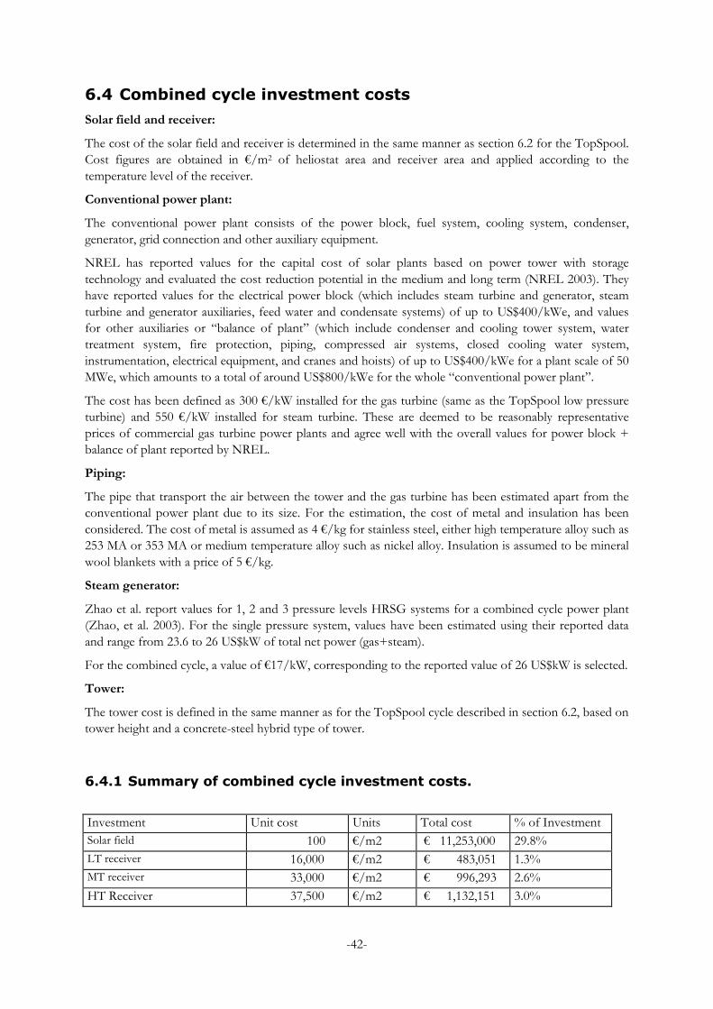
-42-

6.4 Combined cycle investment costs

Solar field and receiver:

The cost of the solar field and receiver is determined in the same manner as section 6.2 for the TopSpool. Cost figures are obtained in €/m2 of heliostat area and receiver area and applied according to the temperature level of the receiver.

Conventional power plant:

The conventional power plant consists of the power block, fuel system, cooling system, condenser, generator, grid connection and other auxiliary equipment.

NREL has reported values for the capital cost of solar plants based on power tower with storage technology and evaluated the cost reduction potential in the medium and long term (NREL 2003). They have reported values for the electrical power block (which includes steam turbine and generator, steam turbine and generator auxiliaries, feed water and condensate systems) of up to US$400/kWe, and values for other auxiliaries or “balance of plant” (which include condenser and cooling tower system, water treatment system, fire protection, piping, compressed air systems, closed cooling water system, instrumentation, electrical equipment, and cranes and hoists) of up to US$400/kWe for a plant scale of 50 MWe, which amounts to a total of around US$800/kWe for the whole “conventional power plant”.

The cost has been defined as 300 €/kW installed for the gas turbine (same as the TopSpool low pressure turbine) and 550 €/kW installed for steam turbine. These are deemed to be reasonably representative prices of commercial gas turbine power plants and agree well with the overall values for power block + balance of plant reported by NREL.

Piping:

The pipe that transport the air between the tower and the gas turbine has been estimated apart from the conventional power plant due to its size. For the estimation, the cost of metal and insulation has been considered. The cost of metal is assumed as 4 €/kg for stainless steel, either high temperature alloy such as 253 MA or 353 MA or medium temperature alloy such as nickel alloy. Insulation is assumed to be mineral wool blankets with a price of 5 €/kg.

Steam generator:

Zhao et al. report values for 1, 2 and 3 pressure levels HRSG systems for a combined cycle power plant (Zhao, et al. 2003). For the single pressure system, values have been estimated using their reported data and range from 23.6 to 26 US$kW of total net power (gas+steam).

For the combined cycle, a value of €17/kW, corresponding to the reported value of 26 US$kW is selected.

Tower:

The tower cost is defined in the same manner as for the TopSpool cycle described in section 6.2, based on tower height and a concrete-steel hybrid type of tower.

6.4.1 Summary of combined cycle investment costs.

Investment Unit cost Units Total cost % of Investment Solar field 100 €/m2 € 11,253,000 29.8% LT receiver 16,000 €/m2 € 483,051 1.3% MT receiver 33,000 €/m2 € 996,293 2.6%

HT Receiver 37,500 €/m2 € 1,132,151 3.0%

-43-

Gas turbine power block 300 €/kW € 13,320,000 35.2% Steam turbine power block 550 €/kW € 7,349,223 19.4% Air pipe 4 €/kg € 136,783 0.4%

Pipe insulation 5 €/kg € 28,058 0.1%

Steam generator 17 €/kWe € 981,958 2.6%

Tower 12,160 €/m € 2,121,149 5.6%

Total cost € 37,801,666 Table 10. Summary of combined cycle power plant investment cost for the 1kW/m2 irradiation case.

Figure 17. Summary of combined cycle power plant investment cost for the 1kW/m2 irradiation case.

Investment Unit cost Units Total cost % of Investment Solar field 100 €/m2 € 17,569,200 39.3% LT receiver 16,000 €/m2 € 483,051 1.1% MT receiver 33,000 €/m2 € 996,293 2.2%

HT Receiver 37,500 €/m2 € 1,132,151 2.5% Gas turbine power block 300 €/kW € 13,320,000 29.8% Steam turbine power block 550 €/kW € 7,348,986 16.4% Air pipe 4 €/kg € 170,912 0.4%

Pipe insulation 5 €/kg € 35,059 0.1%

Steam generator 17 €/kWe € 981,950 2.2%

Tower 12,160 €/m € 2,650,409 5.9%

Total cost € 44,688,013

Table 11. Summary of combined cycle power plant investment cost for the 0.8kW/m2 irradiation case.

29.8%

1.3%

2.6%

3.0%35.2%

19.4%

0.4%

0.1% 2.6%

5.6%

Solar field

LT receiver

MT receiver

HT Receiver

Gas turbine power block

Steam turbine power block

Air pipe

Pipe insulation

Steam generator

Tower

-44-

Figure 18. Summary of combined cycle power plant investment cost for the 0.8kW/m2 irradiation case.

6.5 Combined cycle Operational costs

Operational costs have been defined in the same manner as for the TopSpool cycle.

6.5.1 Operation and maintenance

The data for operation and maintenance costs of the TopSpool cycle described in section 6.3.1 has been obtained from SOLGATE for a second generation combined cycle plant, thus it is also deemed reasonable for the combined cycle evaluation.

A value of 121 k€/y*MW is applied.

6.5.2 Fuel

Natural gas prices vary greatly depending on location, consumption and other factors. A fixed price for natural gas has been obtained from Europe’s Energy Portal (www.energy.eu) for January 2011 for industrial consumers.

A value of 0.027€/kWh, equivalent to approximately US$5/MBTU is set initially and then it is escalated yearly according to the defined inflation rate along with the rest of the operational costs.

6.5.3 Summary of combined cycle operational yearly costs

Operational cost Units Total cost O&M 121.2 k€/y*MW € 7,003,221 Fuel cost 27 €/MWh € 9,542,603 Fuel use 353,430 MWh/year Total € 16,545,824

Table 12. Summary of yearly operational costs for the combined cycle.

39.3%

1.1%

2.2%2.5%

29.8%

16.4%

0.4%0.1%

2.2%

5.9%Solar field

LT receiver

MT receiver

HT Receiver

Gas turbine power block

Steam turbine power block

Air pipe

Pipe insulation

Steam generator

Tower

-45-

7 Results

This section comprises the results for the technical and economical calculations.

7.1 Solar receiver

The calculation for the receivers is described in section 4.4. A flow number or flow area has been calculated based on the values reported by Schwarzbözl, et al. for the SOLGATE project, then used to estimate the increased mass flow that could be circulated through each receiver, allowing for a higher concentration ratio leading to higher receiver power per unit area. This in turn generates a decrease in the necessary receiver area thus reducing the costs of the pressurized volumetric receiver.

The higher pressure of the TopSpool system, coupled with the injection of steam results in a mass flow approximately 8.7 times higher than the values reported for the SOLGATE receivers.

The combined cycle has no steam going through the receiver, however the increased pressure also leads to an increased mass flow of approximately 2.8 times the mass flow from the reference receiver.

The results for the calculation of the flow number K for the reference values, as well as for the TopSpool and combined cycle are presented in Table 13 and Table 14:

Solgate receiver Test 1 Units LT MT HT m 1.357 1.357 1.357 kg/s T 569 766 880 K P 650.0 650.0 650.0 kPa Q 279 169 276 kWth cp air 1.044 1.091 1.117 kJ/kgK K (Flow number) 843.8 979.0 1049.4 m2 Solgate receiver Test 2 LT MT HT m 1.327 1.327 1.327 kg/s T 563 689 886 K P 650.0 650.0 650.0 kPa Q 174 280 217 kWth cp air 1.043 1.072 1.118 kJ/kgK K (Flow number) 820.8 908.0 1029.7 m2

Table 13. Flow number calculation based on reference values by Schwarzbözl, et al.

-46-

TopSpool receiver LT MT HT m 11.135 11.405 11.549 kg/s T 711 871 1031 K P 6275.7 6275.7 6275.7 kPa Q 2,152 2,238 2,323 kWth/receiver cp mix 1.208 1.227 1.257 kJ/kgK K (Flow number) 832.3 943.5 1039.5 n 9 9 9 Receivers

Combined cycle receiver LT MT HT m 3.726 3.827 3.884 kg/s T 735 895 1055 K P 2055.8 2055.8 2055.8 kPa Q

648 666

676

kWth/receiver

cp air 1.087 1.087 1.087 kJ/kgK K (Flow number) 832.3 943.5 1039.5 n 25 25 25 Receivers

Table 14. Flow number and number of receivers calculation results for the TopSpool and combined cycle systems.

The main result is that for the TopSpool system, the increased heat transfer conditions could in theory allow for a receiver up to 3 times smaller than for the combined cycle system. This would in turn have a noticeable effect for the economic calculation although not particularly important because as seen in the definition of installation costs, the cost of the solar receiver amounts to less than 5% of the overall installation cost. However in practice, such reduction in the receiver area would lead to concentration ratios of around 5,000 or higher which are not considered acceptable for the simulation because they have so far not been demonstrated in practice. It is for this reason that the number of receivers has been set as 75 for the combined cycle (25 per cluster), resulting in a concentration ratio of around 1,000 (considering that the heliostat field area is lower for the combined cycle, as shown in the next section), and 57 (19 per cluster) and 72 (24 per cluster) for the two TopSpool cases, resulting in a concentration ratio of around 2,500.

7.2 Solar field

The size of the solar field is determined by the required receiver power, the solar field efficiency, direct normal irradiation and required fluid temperature, as described in section 4.5 and section 5.

As described in section 3, two values for direct normal irradiation have been chosen for evaluation: 0.8 kW/m2 and 1.0 kW/m2. Logically the lower value for irradiation results in a larger solar field necessary to supply the required power. This doesn’t have major implications for the technical calculation, but it is

-47-

important for the economical evaluation because the solar field is the most expensive element in the power plant, so it directly affects the cost of electricity as is shown in section 7.5.

Solar PlantTotal Area Area/unit No units Irradiation Efficiency Heat flux Therm Power Tower height

Radiation m2 m2 kW/m2 kW/m2 kW mGround surface 0.800Solar heliostats 215,985 121 1785 0.800 0.91 0.73 157237 242On receiver 86.9 1.208 1093.0 0.60 0.55 95033To heat exchanger 874.4 0.80 76027Solar plant efficiency 0.44

Table 15. Solar field calculation for TopSpool Cycle at 0.8kW/m2.

Solar PlantTotal Area Area/unit No units Irradiation Efficiency Heat flux Therm Power Tower height

Radiation m2 m2 kW/m2 kW/m2 kW mGround surface 1.000Solar heliostats 172,425 121 1425 1.000 0.91 0.91 156907 216On receiver 68.8 1.208 1377.7 0.60 0.55 94834To heat exchanger 1102.2 0.80 75867Solar plant efficiency 0.44

Table 16. Solar field calculation for TopSpool Cycle at 1.0kW/m2.

Solar PlantTotal Area Area/unit No units Irradiation Efficiency Heat flux Therm Power Tower height

Radiation m2 m2 kW/m2 kW/m2 kW mGround surface 0.800Solar heliostats 175692 121 1452 0.800 0.91 0.73 102323 218On receiver 90.6 0.5 683 0.60 61844To heat exchanger 546 0.80 49475Solar plant efficiency 0.44

Table 17. Solar field calculation for Combined Cycle at 0.8kW/m2.

Solar PlantTotal Area Area/unit No units Irradiation Efficiency Heat flux Therm Power Tower height

Radiation m2 m2 kW/m2 kW/m2 kW mGround surface 1.000Solar heliostats 112530 121 930 1.000 0.91 0.91 102402 174On receiver 90.6 0.5 683 0.60 61892To heat exchanger 547 0.80 49513Solar plant efficiency 0.44

Table 18. Solar field calculation for Combined Cycle at 1.0kW/m2.

In both cases, the increase in irradiation from 0.8 to 1.0 kW/m2 results in a reduction of approximately 20% of required mirror area.

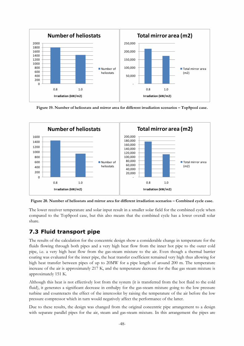
-48-

0

200

400

600

800

1000

1200

1400

1600

1800

2000

0.8 1.0

Irradiation (kW/m2)

Number of heliostats

Number of

heliostats

-

50,000

100,000

150,000

200,000

250,000

0.8 1.0

Irradiation (kW/m2)

Total mirror area (m2)

Total mirror area

(m2)

Figure 19. Number of heliostats and mirror area for different irradiation scenarios – TopSpool case.

0

200

400

600

800

1000

1200

1400

1600

0.8 1.0

Irradiation (kW/m2)

Number of heliostats

Number of

heliostats

-

20,000

40,000

60,000

80,000

100,000

120,000

140,000

160,000

180,000

200,000

0.8 1.0

Irradiation (kW/m2)

Total mirror area (m2)

Total mirror area

(m2)

Figure 20. Number of heliostats and mirror area for different irradiation scenarios – Combined cycle case.

The lower receiver temperature and solar input result in a smaller solar field for the combined cycle when compared to the TopSpool case, but this also means that the combined cycle has a lower overall solar share.

7.3 Fluid transport pipe

The results of the calculation for the concentric design show a considerable change in temperature for the fluids flowing through both pipes and a very high heat flow from the inner hot pipe to the outer cold pipe, i.e. a very high heat flow from the gas-steam mixture to the air. Even though a thermal barrier coating was evaluated for the inner pipe, the heat transfer coefficient remained very high thus allowing for high heat transfer between pipes of up to 20MW for a pipe length of around 200 m. The temperature increase of the air is approximately 217 K, and the temperature decrease for the flue gas steam mixture is approximately 151 K.

Although this heat is not effectively lost from the system (it is transferred from the hot fluid to the cold fluid), it generates a significant decrease in enthalpy for the gas-steam mixture going to the low pressure turbine and counteracts the effect of the intercooler by raising the temperature of the air before the low pressure compressor which in turn would negatively affect the performance of the latter.

Due to these results, the design was changed from the original concentric pipe arrangement to a design with separate parallel pipes for the air, steam and gas-steam mixture. In this arrangement the pipes are

-49-

insulated independently using high insulating material, such as mineral fiber blankets. The calculation for this design results in a much lower heat loss from the gas steam mix. The heat loss to the ambient is around 219 kW for the air pipe, 1,175 kW for the gas steam mix pipe, and 280 kW for the steam pipe, summing up to approximately 1% of the total heat input. The temperature decrease is around 2.5K for the air, 10K for the gas steam mix and 2K for the steam.

The main concern for this design is the availability and cost of the material required for the high temperature pipe (i.e. the pipe that transports the gas-steam mixture from the HPT to the LPT) because the HPT exit temperature is approximately 900°C. It has been determined that special high temperature alloys can withstand these temperatures in normal operation, like 253 MA high temperature steel.

7.4 Cycle performance

Both cycles are modeled on the same gas turbine. The model is formulated in such way that the cycle performance is independent from the irradiation scenario, i.e. the solar field is modeled to provide a predefined thermal input based on the thermodynamic aspects of the fluid. For this reason, this section illustrates the performance of the TopSpool cycle against the combined cycle for any irradiation scenario.

Performance TopSpool cycle Combined cycle

Solar heat input (MW) 76 50

Fuel heat input (MW) 81 72

Solar heat input (%) 48 41

Total turbine power (MW) 83 59

El gross Efficiency % (fuel) 99 80

Net output power (MWel) 80 58

El net Efficiency (%) 51 48

Solar share (%) 25 21

Table 19. Comparison of performance between TopSpool and combined cycle in hybrid mode.

The results suggest that the TopSpool can be as efficient or more than the combined cycle and can obtain higher solar share. Here the main limiting factor for the combined cycle is the temperature level from the receiver which is limited by the material used in the pipe that transports the fluid to the gas turbine, as described in section 5. A more detailed study of materials and cooling options for the pipe system may provide alternatives that could help close the gap in favor of the combined cycle, but it would likely result also in higher installation costs although the pipe cost is not very significant.

In any case, the TopSpool cycle calculation illustrates how the increase in mass flow due to the injection of steam and the higher pressure achieved can significantly increase the power output from the gas turbine system and raise the efficiency when compared to a common gas turbine system.

7.5 Economic evaluation - Levelized Cost of Electricity

The installation and operational costs have been defined in section 6. The results show lower specific investment and operational costs for the TopSpool than for the combined cycle, based on the installed capacity and total annual electricity production.

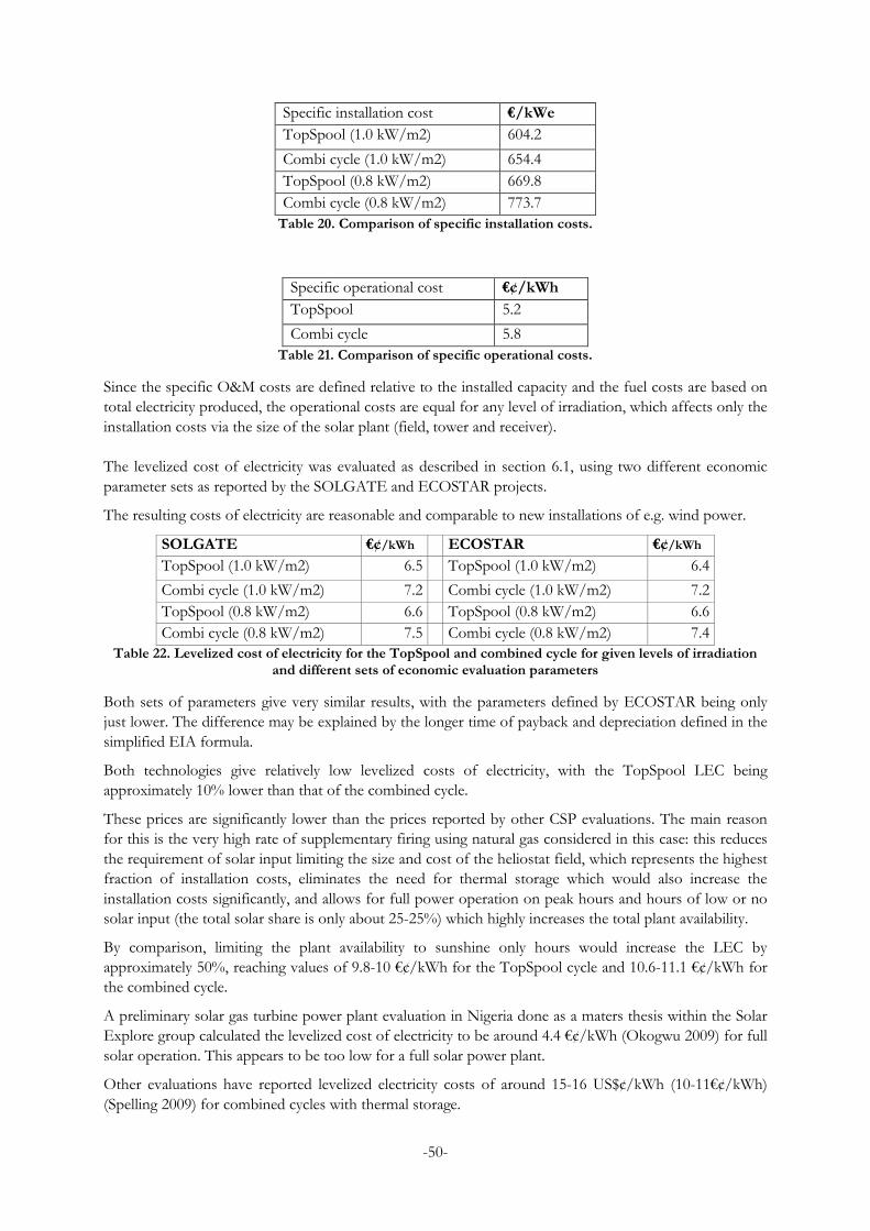
-50-

Specific installation cost €/kWe

TopSpool (1.0 kW/m2) 604.2

Combi cycle (1.0 kW/m2) 654.4 TopSpool (0.8 kW/m2) 669.8 Combi cycle (0.8 kW/m2) 773.7 Table 20. Comparison of specific installation costs.

Specific operational cost €¢/kWh

TopSpool 5.2

Combi cycle 5.8 Table 21. Comparison of specific operational costs.

Since the specific O&M costs are defined relative to the installed capacity and the fuel costs are based on total electricity produced, the operational costs are equal for any level of irradiation, which affects only the installation costs via the size of the solar plant (field, tower and receiver). The levelized cost of electricity was evaluated as described in section 6.1, using two different economic parameter sets as reported by the SOLGATE and ECOSTAR projects.

The resulting costs of electricity are reasonable and comparable to new installations of e.g. wind power.

SOLGATE €¢/kWh ECOSTAR €¢/kWh

TopSpool (1.0 kW/m2) 6.5 TopSpool (1.0 kW/m2) 6.4

Combi cycle (1.0 kW/m2) 7.2 Combi cycle (1.0 kW/m2) 7.2 TopSpool (0.8 kW/m2) 6.6 TopSpool (0.8 kW/m2) 6.6 Combi cycle (0.8 kW/m2) 7.5 Combi cycle (0.8 kW/m2) 7.4

Table 22. Levelized cost of electricity for the TopSpool and combined cycle for given levels of irradiation and different sets of economic evaluation parameters

Both sets of parameters give very similar results, with the parameters defined by ECOSTAR being only just lower. The difference may be explained by the longer time of payback and depreciation defined in the simplified EIA formula.

Both technologies give relatively low levelized costs of electricity, with the TopSpool LEC being approximately 10% lower than that of the combined cycle.

These prices are significantly lower than the prices reported by other CSP evaluations. The main reason for this is the very high rate of supplementary firing using natural gas considered in this case: this reduces the requirement of solar input limiting the size and cost of the heliostat field, which represents the highest fraction of installation costs, eliminates the need for thermal storage which would also increase the installation costs significantly, and allows for full power operation on peak hours and hours of low or no solar input (the total solar share is only about 25-25%) which highly increases the total plant availability.

By comparison, limiting the plant availability to sunshine only hours would increase the LEC by approximately 50%, reaching values of 9.8-10 €¢/kWh for the TopSpool cycle and 10.6-11.1 €¢/kWh for the combined cycle.

A preliminary solar gas turbine power plant evaluation in Nigeria done as a maters thesis within the Solar Explore group calculated the levelized cost of electricity to be around 4.4 €¢/kWh (Okogwu 2009) for full solar operation. This appears to be too low for a full solar power plant.

Other evaluations have reported levelized electricity costs of around 15-16 US$¢/kWh (10-11€¢/kWh) (Spelling 2009) for combined cycles with thermal storage.

-51-

Given these values, the evaluated LEC for this study appears to be reasonable considering the high rate of fossil fuel use (i.e. supplementary firing), the absence of thermal storage and the reduced size of the solar plant.

LEC sensitivity.

An evaluation of the sensitivity of the LEC to variations in the cost of installation or operation gives the following results.

An increase of 10% in installation costs results in an increase of approximately 2% of the LEC.

An increase of 20% in operational costs, including O&M and fuel, clearly has a larger impact, generating an increase of around 16% of the LEC. An increase only in fuel cost would represent an increase of 9% in the LEC.

-52-

8 Conclusions and discussion

Solar field

The evaluation of the solar field in this work has been relatively simple. It has been based only in irradiation and overall efficiency of the field and receiver to deliver a required heat input to the power cycles. No geometrical aspects were considered. The areas and cost of the solar fields are relatively low in comparison with other CSP evaluations in the literature, the main reason for this being the high rate of supplementary firing necessary to reach the required turbine inlet temperatures, and the high power density of the cycles in consideration due to the high pressure levels.

If heliostat mass production can be deployed in the future, and costs drop according to the projections reported in the literature, the total investment costs of CSP plants could be expected to decrease significantly and the cost of solar electricity can become really competitive.

Even though the TopSpool configuration results in relatively large tower sizes compared to the CSP plants in operation today, the literature review has shown that tower development for wind power and studies of future CSP deployment provide enough confidence that towers of this height can be constructed without major technological challenges and at adequate costs. It has also dismissed the initial concern for the weight of the high pressure turbine and electrical equipment and their location on top of the tower.

Solar receiver

Based on the preliminary receiver calculations it has been suggested that the heat transfer characteristics of the gas-steam mixtures could allow for very small solar receivers for CSP plants provided that the structures can be designed to withstand high thermal and pressure transient loads and that higher concentration ratios are proven not to be a very limiting factor in practice.

One area of concern with solar receiver in the cycles is transient operation and especially, load rejection. The long pipes and the receiver cluster store quite a lot of energy in the form of hot pressurized air and steam and heat in metal walls. This energy has to be released in a trip situation in such a way that the turbines do not over speed and the compressors do not run into surge. Further analysis will be required. Blow off valves might be enough, but intercept valves isolating the solar part could be necessary. The risks connected to receiver failures (broken windows, etc.) should be analyzed.

Piping arrangement

The initially proposed arrangement of concentric pipes for the TopSpool configuration resulted in a very high heat transfer inside the system which would have compromised the cycle efficiency, in particular the gas-steam mixture enthalpy going into the low pressure turbine, and the performance of the high pressure compressor due to the high inlet temperature that this would have caused.

A well insulated parallel pipe arrangement should operate well maintaining a low heat loss to the ambient and doesn’t result in significant cost differences.

Plant performance and operation

The thermodynamic calculation suggests that the TopSpool cycle has the potential to reach efficiencies as high as or higher than a combined cycle configuration. Moreover, the possibility to use all of the working media (gas and steam) throughout the whole cycle (i.e. through both expanders), and the high pressure level allow for very high efficiency expectations. Considering that both cycles have been modeled based on the same gas turbine (operating as bottom cycle on the TopSpool and as topping cycle on the combined cycle), the TopSpool generates a higher power output, which contributes to its higher technical and economical performance. A further step might be to make a comparison with a combined cycle that

-53-

delivers the same power output to determine how the increased production of net electricity from the combined cycle can compare to the TopSpool.

In both the TopSpool and combined cycle designs the operation of the plants has so far been neglected. In general, it could be expected that the more thermal flexible TopSpool will allow for quicker start up and load variations, thus probably capturing more solar energy.

Economic performance

A very important technical aspect determining the economic evaluation is the receiver exit temperature. This limits the size of the solar field leading to generally lower investment costs for the combined cycle even though its power block is more expensive due to the steam cycle, which in the beginning was expected to have a significant difference in the investment comparison. However, the receiver temperature also limits the amount of solar heat input to the cycle, which results in overall higher operational costs due to the relatively higher consumption of fuel and the lower power production.

The cost of the receiver turned out to be less important in the overall investment than initially expected. This may lead to the conclusion that more advanced (even if more expensive) receiver designs should be pursued with the objective of increasing the solar performance of the cycle. However, although proven at smaller scales, the technical and operational conditions of the TopSpool (especially the highly transient heat input and the high pressure level) suggest that careful research work is still necessary to determine the viability and potential risks of windowed receivers for large scale application. Detailed mechanical comparison and analysis of windowed against windowless receivers should be explored to envision the best way forward.

The calculated cost of electricity looks promising. It can be expected that both the TopSpool and combined cycle will be competitive with other technologies in the medium to long term. Again, the main factor contributing to the low LEC in the evaluation is the high rate of supplementary firing which allows for stable operation and high power output levels even in times of no solar irradiation, but a reduction in the operation hours (i.e. an increase in the solar share to around 50% by limiting the operation time to sunshine only hours) still results in reasonably low LEC prices for CSP plants. Further work may include technical and economical optimization, with the objective of determining if the TopSpool can continue to surpass the technical and economical performance of a combined cycle with the same power output.

It should be noted that the main objective was to make a sound comparison of the TopSpool with the combined cycle for this particular application. Some elements in the investment calculation have been omitted, like cost of land and land preparation, engineering and development costs for non-standard equipment (such as the receiver), but these would not be expected to significantly change the investment scenarios and would likely have the same relative impact on the cost of investment for both systems. Moreover, as the sensitivity analysis suggests, the cost of electricity appears to be much more sensitive to operational costs and yearly electricity production.

-54-

Bibliography

Engström, Staffan, Tomas Lyrner, Manouchehr Hassanzadeh, Thomas Stalin, and John Johansson. Tall towers for large wind turbines. Technical report, Elforsk, 2010.

EUROPEAN COMMISSION - Directorate-General for Research. "SOLGATE Solar hybrid gas turbine electric power system." 2005.

EUROTURBINE AB. "The future carbon free power plant." 2009.

Heller, Peter, et al. "Test and evaluation of a solar powered gas turbine system." Solar Energy 80 (2006): 1225-1230.

International Energy Agency. "Guidelines for the economic analysis of renewable energy technology applications." 1991.

Jonkman, J., S. Butterfield, W. Musial, and G. Scott. Definition of a 5-MW Reference Wind Turbine for Offshore System Development. Denver: National Renewable Energy Laboratory, 2009.

Jonsson, Maria, and Jinyue Yan. "Humidified gas turbines - a review of proposed and implemented cycles." Energy (ELSEVIER) 30 (2005): 1030 - 1078.

Kribus, Abraham. "A high-efficiency triple cycle for solar power generation." Solar Energy 72, no. 1 (2002): 1-11.

Kribus, Abraham, et al. "A MULTISTAGE SOLAR RECEIVER: THE ROUTE TO HIGH TEMPERATURE." Solar Energy, 1999: 3-11.

Norlund, Samuel, and Sarah Trouvé. Solar Receiver Design and Integration in a Gas-Turbine Cycle. KTH, 2010.

NREL. Assessment of Parabolic Trough and Power Tower Solar Technology Costs and Performance Forecasts. Technical report., Golden, Colorado.: National Renewable energy Laboratory, 2003.

Pitz-Paal, Robert, Jürgen Dersch, and Barbara Milow. European Concentrated Solar Thermal Road Mapping. Technical Report, ECOSTAR - European Comission, 2005.

SANDIA. Heliostat Cost Reduction Study. Technical report, Albuquerque: Sandia National Laboratories, 2007.

Schwarzbözl, Peter, et al. "Solar gas turbine systems: Design, cost and perspectives." Solar Energy 80 (2006): 1231-1240.

SIEMENS. "SGT-800 Siemens." Siemens Global Website. 2009. http://www.energy.siemens.com/co/en/power-generation/gas-turbines/sgt-800.htm (accessed 02 03, 2011).

SOLHYCO. SOLHYCO - Solar Hybrid and Cogeneration Plants. 2011. http://www.greth.fr/solhyco/ (accessed May 5, 2011).

SOLUGAS. SOLUGAS. Solar Up-Scale Gas Turbine System. 2009. http://www.solugas.com (accessed May 5, 2011).

Spelling, James. Thermo-Economic Optimisation of Solar Tower Thermal Power Plants. Masters Thesis, Lausanne: École Polytechnique Fédérale de Lausanne, 2009.

Zhao, Yongjun, Hongmei Chen, Mark Waters, and Dimitri N. Mavris. "MODELING AND COST OPTIMIZATION OF COMBINED CYCLE HEAT RECOVERY GENERATOR SYSTEMS." Proceedings of ASME Turbo Expo 2003. Atlanta, Georgia: ASME, 2003.

-55-

Appendix 1.

Two Microsoft excel files are attached as appendixes including the technical and economical calculations for the TopSpool cycle and Combined cycle:

Solar_TopCycle_V3.xls

SGT800_solar_combi.xls