www.sciencemag.org/content/341/6153/1238670/suppl/DC1

Supplementary Materials for

Soil Diversity and Hydration as Observed by ChemCam at Gale Crater, Mars

P.-Y. Meslin,* O. Gasnault, O. Forni, S. Schröder, A. Cousin, G. Berger, S. M. Clegg, J. Lasue, S. Maurice, V. Sautter, S. Le Mouélic, R. C. Wiens, C. Fabre, W. Goetz, D. Bish, N. Mangold,

B. Ehlmann, N. Lanza, A.-M. Harri, R. Anderson, E. Rampe, T. H. McConnochie, P. Pinet, D. Blaney, R. Léveillé, D. Archer, B. Barraclough, S. Bender, D. Blake, J. G. Blank, N. Bridges, B. Clark, L. DeFlores, D. Delapp, G. Dromart, M. D. Dyar, M. Fisk, B. Gondet, J. Grotzinger,

K. Herkenhoff, J. Johnson, J.-L. Lacour, Y. Langevin, L. Leshin, E. Lewin, M. B. Madsen, N. Melikechi, A. Mezzacappa, M. A. Mischna, J. E. Moores, H. Newsom, A. Ollila, R. Perez,

N. Renno, J.-B. Sirven, R. Tokar, M. de la Torre, L. d’Uston, D. Vaniman, A. Yingst, MSL Science Team

*Corresponding author. E-mail: pmeslin@irap.omp.eu

Published 27 September 2013, Science 341, 1238670 (2013) DOI: 10.1126/science.1238670

This PDF file includes:

Supplementary Text

Figs. S1 to S4

MSL Science Team Author List

2

Supplementary Text Data processing and ICA-based Cluster Analysis

As described in (36), the data are pre-processed to remove noise, continuum, and the ambient light signal. The spectra are normalized by the total intensity in each of the three spectrometers, and the instrument response is corrected. A wavelength calibration is also applied. The only difference with the procedure as applied to rocks is that the spectra from the first five shots on each target were kept in this study because in an unconsolidated material, they are already representative of the soil composition, and dust itself can also be viewed as a soil component. The data are then processed through an Independent Component Analysis (ICA) to determine the peaks with the greatest variation within the data set, which may serve as proxies for elemental abundances (see below). Here we retain the ICA components corresponding to Al, Fe, H, K, Mg, Na, O, Si, Ti, Ca (elemental lines) and tentatively CaO (molecular band). The components serve as input to a clustering algorithm. We adopt a divisive algorithm by (79), which starts with the entire dataset and iteratively subdivides the data into two subgroups in order to determine the main data structures. This hierarchical method is also appropriate to find the optimal number of clusters and reveals relations between a parent unit and its sub-units.

Independent Component Analysis (ICA) is a Multivariate Analysis technique that

comes from developments in the Blind Source Separation research. The goal of ICA is to estimate h source signals, assumed to be stationary and independent, using n observed signals that are independent unknown mixing of the source signals. ICA, like PCA (Principal Component Analysis), transforms the original representative space by searching for directions in a new space, so that the resulting vectors are independent, and not solely uncorrelated (80). ICA is then a method of linear transformation in which the representation is the one that minimizes the statistical dependence of the components. This is achieved using a criterion that is related to the information entropy theory that gives back the statistical independence assuming that the data follow a non-Gaussian distribution. The choice of the method is justified because, in nature, the sources we are searching for are never distributed randomly. Moreover, searching for sources that are mutually independent, and not solely uncorrelated, is much more discriminant. We have used the Joint Approximate Diagonalization of Eigenmatrices method (JADE) algorithm (81), which is an orthogonal ICA method and, like most mainstream ICA techniques, it exploits higher order statistics related to the fourth order cross cumulants to maximize the non-gaussianity of the sources. Once the independent components have been obtained, it is easy to compute the score of each spectra in that reference frame; it is simply the covariance between the spectra and the independent components. Quantitative predictions of abundances with the Partial Least Square technique abundances and difference of normalization with respect to the APXS

3

Quantitative predictions for the composition of ChemCam targets are obtained with a Partial Least Squares (PLS) technique also known as PLS2. PLS2 is a multivariate analysis technique that has been successfully used for LIBS analysis (35, 82). Using a calibration database of 66 standards of known compositions and analyzed by ChemCam under laboratory conditions replicating Mars prior to flight, it is possible to apply the PLS2 regression to the spectral data for quantitative predictions (36). PLS2 makes use of an iterative PCA-like dimensionality reduction procedure to find the largest variance directions in the matrix of the standards ChemCam spectra as well as in the matrix of the standards compositions, and modifies both directions found at each step so as to maximize their correlation. The regression is then modeled using the reduced matrices. The accuracy of the method is calculated by taking the root mean square of error prediction (RMSEP) from a leave-one-out cross-validation procedure on the training set formed from the database of standards. Given in units of the predicted quantity, it is related to the standard deviation of the errors of prediction within the model and gives an indication of their distribution. The number of principal components for the PLS2 model was taken to be 9 for which the RMSEP is one standard deviation above the minimum global RMSEP value for all elements (36).

The techniques used to determine ChemCam PLS2 predicted abundances and APXS

abundances data do not use the same normalization. APXS composition values are given with a total of 100 wt% by default. However, the APXS measurement technique is not readily sensitive to light elements such as hydrogen or carbon which have been detected in the soils by SAM to a level of ∼ 3.5 wt% (H2O + CO2). On the other hand, the ChemCam PLS2 prediction method does not force the total of abundances to be equal to 100 wt%, allowing the prediction of a possible unknown component in the composition of the sample, every other element being predicted to its actual sample content. If ∼ 3.5 wt% of light elements as determined by SAM are present in the Martian soil, then taking it into account in the APXS total would decrease the value of major elements determined by the APXS by up to 1.5-2 wt%, most importantly in the case of SiO2. This difference in normalization may explain part of the difference observed between APXS and ChemCam PLS2 abundances. Qualitative analysis of grain-size

In order to identify grains whose size is at least of the order of the LIBS spot (350 – 550 µm) (i.e., grains that are sufficiently large to withstand the blasting effect or soil disturbance caused by the laser shock wave for at least a few laser shots, and thus larger than the scale of the LIBS spot), and referred to as “coarse”, three features have been checked:

1) Visualization of RMI images: The points where ChemCam shoots are usually known with good precision based on RMI images. Moreover, at least one RMI is taken before (pre-RMI) and after (post-RMI) the LIBS activity. If pebbles are seen in the LIBS spot in both pre- and post-RMIs (this is the case for Beaulieu point #2, #3, #4 in Fig. 1D), then it can be inferred that the corresponding spectra are fully representative of these individual grains (with usually the first

4

few shots coming from the dust), just like for rock analysis. These grains are not smaller than 1 to a few mm. However, some ∼ 1 mm grains are also often seen to be moved around by the interaction with the laser, and some coarse grains could also be buried and not visible even in the post-RMI images (this is believed to occur often), so this first filter is not sufficient.

2) The PLS2 technique can also be applied on every single laser shot observation, to derive the sample composition for that shot. Clear simultaneous discontinuities in the composition of several elements with depth indicate that the laser penetrated into a different medium, which is likely an indicator for the presence of a “coarse” grain.

3) However, it would be conceivable that two layers (or more) of fine-grained material would give a similar discontinuity in composition. Therefore, we also checked that the total intensity of the spectra is consistent with that of an unconsolidated fine-grained powder, or to that of a hard, consolidated material. In the former case, the dispersion of the intensity is typically large, while in the latter case, it shows little fluctuations. When such a drop in intensity fluctuations is encountered at the same time as a compositional discontinuity, the few shots concerned are labelled as stemming from a “coarse” grain in Fig. 3B. They can be only “3 to 4 shots wide”, but also more than “25 shots wide” (most soil acquisitions were 30 shots deep).

Variability within the Rocknest ripple

To investigate differences of chemical composition between the interior of the trench dug in the Rocknest ripple and its armor (Fig. 1B, Fig. S2), the dataset has been split into two categories: 1) all the shots acquired in the interior of the trench on one side (“Interior of the trench”), 2) all the shots acquired on the bedform armor on the other (“Top of the ripple”). These two categories are shown in Fig. S3, where Na2O+K2O shot-by-shot concentrations are plotted versus SiO2. Although the two categories overlap, the second category is seen to extend to larger Na2O+K2O and SiO2 concentrations than the first category. However, given the relatively small size of the ∼ 1 mm-sized grains covering the bedform, they are likely to be dispersed by the laser shock wave, as observed on RMI images (Fig. 1B). As a result, even the data acquired on the top of the ripple are diluted with some underlying, fine-grained material. Similarly, Mastcam images show that many coarse grains fell into the trench when it was scooped (Fig. S2-a). These grains, if hit by the laser, would fall in the category “Interior of the trench”. Moreover, during the formation of the ripple, similar grains have probably been incorporated in the aeolian bedform. This would also result in a mixing between the two populations. Therefore, the shots that have been identified as part of a “coarse” grain in either of the two former categories have been superimposed in Fig. S3. Most of the “green” data points that fall in the upper part of the “orange” cloud are seen to be “coarse” grains, while most of the “orange” data points falling in the lower part of the “green” cloud do not indicate the presence of such grains.

5

Analysis of the Hydrogen line

As illustrated in Fig. S4, the ChemCam LIBS raw data (blue dashed line) are processed subtracting a so-called dark spectrum (dot-dashed orange line) measured for the same integration time as the active LIBS spectra but without the laser, to account for reflected sunlight, pattern noise and counts due to thermal dark current. The dark spectrum measured on Mars depends highly on the target type and solar irradiation properties and was measured after the LIBS analysis. The most intense hydrogen line at 656.5 nm is partly superimposed by a carbon line at 658.0 nm that is present with almost constant intensity in all the LIBS data due to the CO2 dominated atmosphere on Mars. To investigate variations of the hydrogen signal intensity, both emission lines in the net signal (solid purple line) were fitted simultaneously with Lorentzian line shapes. The trends are given as signal (amplitude from fit) to background ratios (SBRs), where the background is defined by the offset of the spectrum due to continuum radiation in a peak free wavelength interval close to the hydrogen line, as shown by the purple arrow. Discussion on the sensitivity of the hydrogen analysis

It is important to address the question of the sensitivity of the hydrogen analysis discussed in the main text, so as to give an idea of what level of variation in hydrogen content we would have been able to detect. There are two possible approaches to the problem of H quantification by the LIBS technique: laboratory calibration using standards with known hydrogen abundances and a similar instrumental setup, or direct in situ calibration using H2O abundances measured by other instruments, which on Mars is limited to SAM analyses of soils and grinded rocks. Since laboratory calibration has not been conducted yet for hydrogen, we used the second approach, based on SAM soil analyses at Rocknest. Although more limited in terms of accuracy than laboratory measurements (because SAM has its own uncertainties), it has the advantage of being conducted directly with the Flight Model of the instrument and on Mars, thus avoiding problems of reproducibility. Since a single, average H2O abundance was estimated by SAM, we rely on a few assumptions. We discuss this approach in the following to provide an estimate of our sensitivity.

First, a H line is clearly identified in soils above background, so detection of water is

not an issue. At the level of hydration seen here, the H line is not saturating. Moreover, in the above analysis, we compared materials that were very similar in texture and composition, so the matrix effects affecting the laser coupling are minimized when differences are investigated. Therefore, we are confident that the hydrogen S/B ratio increases with abundance. A linear increase of the H peak intensity with water content was observed in the laboratory work by (83) on lunar samples (with H2O contents up to 3.6 wt%), even though it was obtained on a heterogeneous set of samples. Therefore, we assume that the S/B ratio increases linearly with hydrogen abundance in this range of water contents.

6

If no H was present in the soil, our analysis process would still return a value for H, in the noise of the method (be it ICA or univariate peak analysis). Such a “blank” can be estimated by applying our routines to targets where H is known to be absent, for instance our onboard calibration targets. The S/B ratio for these targets is about ∼ 0.08 ± 0.04, while for Cluster 1 soils, the mean S/B ratio is 1.1 ± 0.3, as seen in Fig. 6B. This sigma value is here for a set of 62 samples. In Fig. 6B, the largest 1σ error bars are from populations with a smaller number of samples (<62, because some spectra associated with “coarse” grains buried at some depth were removed from the analysis, discarding the sample for those specific shot numbers). We can further reduce the value of σ by providing an estimate of the S/B value for the bulk topmost millimeters (30 shots), because no significant variations is seen in this dataset with shot number (Fig. 6B). The uncertainty on the average value for the 30 shots (S/B = 1.09) is σ = 0.07. Therefore, our ability to detect variations really depends on the size of the populations we are comparing, and on our ability to select these populations from physical and/or chemical considerations (each population should be homogeneous). Our large dataset is an advantage to this respect. For a single point analysis (e.g., Crestaurum_day or Crestaurum_night), the S/B is 1.06 ± 0.25, so the point-to-point comparison has a larger detection threshold (i.e., positive detection of a significant difference).

If we assume a linear variation of the H line intensity as a function of abundance, as

developed above, we can assume a linear scale between our blank (H2O = 0 wt%, (S/B)CCAM = 0.08) and the abundance measured by SAM ((H2O)SAM = 2.25 wt% , (S/B)CCAM = 1.1). Therefore, we can define an upper limit at a 95% confidence level for the observed variations as: net difference + 1.645 × σobs (this formula is justified because the sigmas of the two observations are very similar). For the day/night experiment, this gives an upper limit of ∼ 0.45 (in units of S/B, i.e. dimensionless). This translates to a water content of 0.45/(1.06-0.08) × (H2O)SAM = 1.1 wt%. When comparing large datasets (interior of the trench vs. undisturbed soil), the lower σobs lowers the upper limit for the difference to ∼ 0.11, which translates to ∼ 0.25 wt%. Qualitatively, we can also say that we are seeing gradual differences in H-component or H-line intensity between soils that are probably characterized by various degrees of mixing (Fig. 5). Therefore, it is reasonable to assume that we could distinguish differences of a fraction of a few units of (H2O)SAM.

To constrain quantitatively the variability with time of the exposed material (Fig.

6C), we can calculate the uncertainty on the slope of a linear fit through the data points. The idea is that if the slope was larger than about twice its uncertainty, we could conclude that a decrease with time was probably detected. Here, the slope is 0.004 ± 0.010 (in units of (S/B)/sol), hence, if the slope was twice its uncertainty (0.02), the difference seen over 25 sols would have been 25 × 0.02 = 0.5 (in units of (S/B)). If we take this value as an upper limit of the difference we are not seeing, this translates to ∼ 1.1 wt%. However, we can also argue that since the interior of the trench is similar to undisturbed material within 0.25 wt%, if exposed, there is no physical reason why it would become less hydrated than the undisturbed, exposed material. Therefore, the desiccation was probably less than 0.25 wt%.

7

Discussion on the temperature dependence of the isotherms.

The surface temperature on sol 74 around noon was >273 K and on sol 75 at 4:30 am LMST was ∼ 195 K. By lack of water adsorption isotherms measured on Martian analogs at these temperatures, the isotherms obtained by (67) need to be extrapolated to lower and higher temperatures. Note that these isotherms are expressed as a function of relative humidity with respect to the saturated vapor pressure of ice. The dependence of an adsorption isotherm (expressed as adsorbed mass as a function of relative humidity) on temperature depends on the isosteric heat of sorption (differential molar enthalpy of sorption), according to the Clausius-Clapeyron equation (84):

( )( )21

21sublim

1

2lnTTR

TTHQ

RH

RH isost −−=

(1)

where 0/ ppRH = , with p the vapor pressure of the sorbed water and p0 the vapor

pressure of ice at the temperature T in question, Qisost is the isosteric heat of sorption, and Hsublim the partial molar enthalpy of water ice.

The isosteric heat of sorption Qisost (θ) depends on the surface coverage θ of the substrate by the sorbed species, and usually increases as the surface coverage decreases for hydrophilic substrates. If Qisost (θ) is greater than the sublimation enthalpy of water ice Hsublim (51.059 kJ mol-1 at 0 °C), the relative humidity leading to a fixed amount of adsorbed water will decrease with decreasing temperature. This also means that for a given relative humidity, the amount of adsorbed water will increase with decreasing temperature. If the isosteric heat of adsorption is equal to the sublimation enthalpy of water ice, then the isotherm is invariant with changes in temperature (as long as (Qisost-Hsublim) varies little with temperature, assumption made in the above equation). Finally, if it is lower, the amount of adsorbed water will decrease with decreasing temperature.

Therefore, if Qisost(θ) > Hsublim for the degree of coverage θ obtained at 243 K (temperature at which the isotherms were measured), the amount of water vapor adsorbed at 195 K (273 K) at RH = 0.3 will be greater (lower) than the amount of water vapor adsorbed at 243 K and the difference of slopes between the two curves in Fig. 7 will be greater. The SSA needed to account for a difference of 1.1 wt% between day and night time will thus be smaller. In that case, the upper limit of the SSA obtained with curves at 243 K remains an even safer upper limit of the SSA that would have been obtained if the isotherms at T = 190 K and 273 K were available.

Extrapolation of the isotherms obtained on montmorillonite at 0°C and 20°C by Mooney et al. (1952) (84) to Martian temperatures showed that the amount of water adsorbed at RH = 0.3 is almost invariant with temperature (85). Curves of Qisost as a function of relative humidity or amount adsorbed obtained for allophane (86), nontronite (87) and different types of zeolites (87-89, and references therein) show that the condition Qisost(θ) ≥ Hsublim is met at RH = 0.3. Fanale and Cannon (1974) (78) measured adsorption isotherms of ground Vacaville basalt at 25°C, 0°C and -20°C and found the isotherms to superimpose very well when expressed as a function of relative humidity with respect to liquid or supercooled liquid saturated vapor pressure. Note that the mass adsorbed at -20°C at RH=0.24 (i.e., RH=0.3 with respect to the saturated pressure of ice)

8

falls on the same linear trend as the data taken from Pommerol et al. (2009) (67) (Fig. 7). The result of Fanale and Cannon (1974) (78) suggests that the isosteric heat of adsorption for that material is close to the water enthalpy of vaporization (Hvap = 45.051 kJ mol-1 at 0°C). Taking Qisost - Hsublim = Hliq - Hsublim = - 6 kJ mol-1, the amount adsorbed at 195 K (273 K) can be read on the isotherms of Pommerol et al. (2009) (67) by considering a relative humidity RH = 14% instead of 30%, according to Clausius-Clapeyron equation, and the amount adsorbed at 273 K at noon would be essentially the same as that at 243 K. This would decrease the difference between the two slopes in Fig. 7 to ∼ 0.024 wt%/(m2.g-1) and thus increase our estimate of the upper limit of the SSA to ∼ 45 m2.g-1.

In this analysis, the dependence of kinetic factors on temperature have not been considered. Beck et al. (2010) (69) have shown that adsorption equilibrium at 243 K for the samples analyzed by Pommerol et al. (2009) (67) is relatively fast with respect to the diurnal cycle. Kinetic factors at 195 K are unknown, but if a simple Langmuir type of adsorption can be assumed, then the characteristic equilibration time scale τ = (ka + kd)

-1 ≈ (ka)

-1 ≈ 200 seconds at low temperatures (69), where ka and kd are the characteristic time constants for adsorption and desorption, respectively. If intra-grain diffusion is actually the limiting factor, kinetics may be much slower. Slow intra-grain diffusion (e.g., requiring activation energy) could be the reason for not seeing day/night differences. Effective diffusion in the inter-grain porosity, however, should not be problematic because the first shots analyzed by ChemCam are very surficial (each shot probes a fraction of a millimeter).

9

Fig. S1. Detection of “coarse” grains in the soil targets. Detected grains are indicated with dashed lines in each case. A) Shot-by-shot Partial Least Square composition (only SiO2 is represented here for clarity) for three examples of ablation points; B) Shot-by-shot total intensity of the spectra for the corresponding points. Discontinuities in composition and groups of shots with small shot-to-shot intensity fluctuations are attributed to the presence of grains likely to be at least the size of the LIBS spot. Crestaurum_day, on the other hand, is a fine-grained aeolian soil (Fig. 1C), and exhibits large shot-to-shot fluctuations.

0

10

20

30

40

50

60

70

80

1 3 5 7 9 11 13 15 17 19 21 23 25 27 29 31 33 35 37 39 41 43 45 47 49

SiO

2 (

wt%

)

Shot number

Murky #2

Grain

0

5

10

15

20

25

30

35

40

45

1 3 5 7 9 11 13 15 17 19 21 23 25 27 29

SiO

2 (

wt%

)

Shot number

Crestaurum (day)

0

10

20

30

40

50

60

1 3 5 7 9 11 13 15 17 19 21 23 25 27 29

SiO

2 (

wt%

)

Shot number

Akaitcho #7

Grain

A B

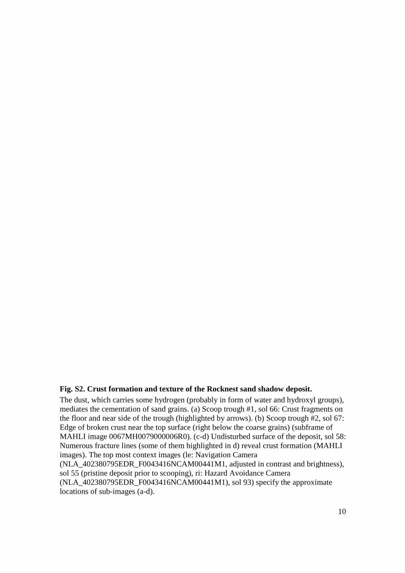
Fig. S2. Crust formation The dust, which carries sommediates the cementation othe floor and near side of thEdge of broken crust near tMAHLI image 0067MH00Numerous fracture lines (simages). The top most con(NLA_402380795EDR_F0sol 55 (pristine deposit prio(NLA_402380795EDR_F0locations of sub-images (a

on and texture of the Rocknest sand shadow dsome hydrogen (probably in form of water and n of sand grains. (a) Scoop trough #1, sol 66: Cf the trough (highlighted by arrows). (b) Scoop ar the top surface (right below the coarse grains0079000006R0). (c-d) Undisturbed surface of t (some of them highlighted in d) reveal crust foontext images (le: Navigation Camera F0043416NCAM00441M1, adjusted in contrasrior to scooping), ri: Hazard Avoidance CamerF0043416NCAM00441M1), sol 93) specify th

(a-d).

10

w deposit. d hydroxyl groups),

: Crust fragments on op trough #2, sol 67: ins) (subframe of of the deposit, sol 58: formation (MAHLI

trast and brightness), era the approximate

11

Fig. S3. Chemical variability in the Rocknest sand shadow. Partial Least Square alkali and SiO2 compositions for the population of spectra obtained from the interior and from the top of the trench. Symbols with dark outlines correspond to spectra that were identified as stemming from “coarse” grains, following the method described in the previous section. Epworth #5, Epworth3 #3, Kenyon #8 and Epworth2 #3 are specific coarse grains mentioned in the main text.

0

1

2

3

4

5

6

7

20 30 40 50 60 70 80

Na

2O

+ K

2O

(w

t%)

SiO2 (wt%)

Top of ripple

"Coarse grains" detected on top

Interior of trench

"Coarse grains" detected in the trench

Epworth #5

Epworth3 #3

Kenyon #8

Epworth2 #3

12

Fig. S4. Hydrogen signal processing. See text for details. This example corresponds to the target Crestaurum (Fig. 1C).

Mars Science Laboratory (MSL) Science Team Aalto University Osku Kemppinen Applied Physics Laboratory (APL) at Johns Hopkins University Nathan Bridges, Jeffrey R. Johnson, Michelle Minitti Applied Research Associates, Inc. (ARA) David Cremers Arizona State University (ASU) James F. Bell III , Lauren Edgar, Jack Farmer, Austin Godber, Meenakshi Wadhwa, Danika Wellington Ashima Research Ian McEwan, Claire Newman, Mark Richardson ATOS Origin Antoine Charpentier, Laurent Peret Australian National University (ANU) Penelope King Bay Area Environmental Research Institute (BAER) Jennifer Blank Big Head Endian LLC Gerald Weigle Brock University Mariek Schmidt Brown University Shuai Li, Ralph Milliken, Kevin Robertson, Vivian Sun California Institute of Technology (Caltech) Michael Baker, Christopher Edwards, Bethany Ehlmann, Kenneth Farley, Jennifer Griffes, John Grotzinger, Hayden Miller, Megan Newcombe, Cedric Pilorget, Melissa Rice, Kirsten Siebach, Katie Stack, Edward Stolper Canadian Space Agency (CSA) Claude Brunet, Victoria Hipkin, Richard Léveillé, Geneviève Marchand, Pablo Sobrón Sánchez Capgemini France Laurent Favot

Carnegie Institution of Washington George Cody, Andrew Steele Carnegie Mellon University Lorenzo Flückiger, David Lees, Ara Nefian Catholic University of America Mildred Martin Centre National de la Recherche Scientifique (CNRS) Marc Gailhanou, Frances Westall, Guy Israël Centre National d'Etudes Spatiales (CNES) Christophe Agard, Julien Baroukh, Christophe Donny, Alain Gaboriaud, Philippe Guillemot, Vivian Lafaille, Eric Lorigny, Alexis Paillet, René Pérez, Muriel Saccoccio, Charles Yana Centro de Astrobiología (CAB) Carlos Armiens‐Aparicio, Javier Caride Rodríguez, Isaías Carrasco Blázquez, Felipe Gómez Gómez , Javier Gómez-Elvira, Sebastian Hettrich, Alain Lepinette Malvitte, Mercedes Marín Jiménez, Jesús Martínez-Frías, Javier Martín-Soler, F. Javier Martín-Torres, Antonio Molina Jurado, Luis Mora-Sotomayor, Guillermo Muñoz Caro, Sara Navarro López, Verónica Peinado-González, Jorge Pla-García, José Antonio Rodriguez Manfredi, Julio José Romeral-Planelló, Sara Alejandra Sans Fuentes, Eduardo Sebastian Martinez, Josefina Torres Redondo, Roser Urqui-O'Callaghan, María-Paz Zorzano Mier Chesapeake Energy Steve Chipera Commissariat à l'Énergie Atomique et aux Énergies Alternatives (CEA) Jean-Luc Lacour, Patrick Mauchien, Jean-Baptiste Sirven Concordia College Heidi Manning Cornell University Alberto Fairén, Alexander Hayes, Jonathan Joseph, Steven Squyres, Robert Sullivan, Peter Thomas CS Systemes d'Information Audrey Dupont Delaware State University Angela Lundberg, Noureddine Melikechi, Alissa Mezzacappa

Denver Museum of Nature & Science Julia DeMarines, David Grinspoon Deutsches Zentrum für Luft- und Raumfahrt (DLR) Günther Reitz eINFORMe Inc. (at NASA GSFC) Benito Prats Finnish Meteorological Institute Evgeny Atlaskin, Maria Genzer, Ari-Matti Harri, Harri Haukka, Henrik Kahanpää, Janne Kauhanen, Osku Kemppinen, Mark Paton, Jouni Polkko, Walter Schmidt, Tero Siili GeoRessources Cécile Fabre Georgia Institute of Technology James Wray, Mary Beth Wilhelm Géosciences Environnement Toulouse (GET) Franck Poitrasson Global Science & Technology, Inc. Kiran Patel Honeybee Robotics Stephen Gorevan, Stephen Indyk, Gale Paulsen Imperial College Sanjeev Gupta Indiana University Bloomington David Bish, Juergen Schieber Institut d'Astrophysique Spatiale (IAS) Brigitte Gondet, Yves Langevin Institut de Chimie des Milieux et Matériaux de Poitiers (IC2MP) Claude Geffroy Institut de Recherche en Astrophysique et Planétologie (IRAP), Université de Toulouse David Baratoux, Gilles Berger, Alain Cros, Claude d’Uston, Olivier Forni, Olivier Gasnault, Jérémie Lasue, Qiu-Mei Lee, Sylvestre Maurice, Pierre-Yves Meslin, Etienne Pallier, Yann Parot, Patrick Pinet, Susanne Schröder, Mike Toplis

Institut des Sciences de la Terre (ISTerre) Éric Lewin inXitu Will Brunner Jackson State University Ezat Heydari Jacobs Technology Cherie Achilles, Dorothy Oehler, Brad Sutter Laboratoire Atmosphères, Milieux, Observations Spatiales (LATMOS) Michel Cabane, David Coscia, Guy Israël, Cyril Szopa Laboratoire de Géologié de Lyon : Terre, Planète, Environnement (LGL-TPE) Gilles Dromart Laboratoire de Minéralogie et Cosmochimie du Muséum (LMCM) François Robert, Violaine Sautter Laboratoire de Planétologie et Géodynamique de Nantes (LPGN) Stéphane Le Mouélic, Nicolas Mangold, Marion Nachon Laboratoire Génie des Procédés et Matériaux (LGPM) Arnaud Buch Laboratoire Interuniversitaire des Systèmes Atmosphériques (LISA) Fabien Stalport, Patrice Coll, Pascaline François, François Raulin, Samuel Teinturier Lightstorm Entertainment Inc. James Cameron Los Alamos National Lab (LANL) Sam Clegg, Agnès Cousin, Dorothea DeLapp, Robert Dingler, Ryan Steele Jackson, Stephen Johnstone, Nina Lanza, Cynthia Little, Tony Nelson, Roger C. Wiens, Richard B. Williams Lunar and Planetary Institute (LPI) Andrea Jones, Laurel Kirkland, Allan Treiman Malin Space Science Systems (MSSS) Burt Baker, Bruce Cantor, Michael Caplinger, Scott Davis, Brian Duston, Kenneth Edgett, Donald Fay, Craig Hardgrove, David Harker, Paul Herrera, Elsa Jensen, Megan R. Kennedy, Gillian Krezoski, Daniel Krysak, Leslie Lipkaman, Michael Malin, Elaina McCartney, Sean McNair, Brian Nixon, Liliya Posiolova, Michael Ravine, Andrew Salamon, Lee Saper, Kevin Stoiber, Kimberley Supulver, Jason Van Beek, Tessa Van Beek, Robert Zimdar

Massachusetts Institute of Technology (MIT) Katherine Louise French, Karl Iagnemma, Kristen Miller, Roger Summons Max Planck Institute for Solar System Research Fred Goesmann, Walter Goetz, Stubbe Hviid Microtel Micah Johnson, Matthew Lefavor, Eric Lyness Mount Holyoke College Elly Breves, M. Darby Dyar, Caleb Fassett NASA Ames David F. Blake, Thomas Bristow, David DesMarais, Laurence Edwards, Robert Haberle, Tori Hoehler, Jeff Hollingsworth, Melinda Kahre, Leslie Keely, Christopher McKay, Mary Beth Wilhelm NASA Goddard Space Flight Center (GSFC) Lora Bleacher, William Brinckerhoff, David Choi, Pamela Conrad, Jason P. Dworkin, Jennifer Eigenbrode, Melissa Floyd, Caroline Freissinet, James Garvin, Daniel Glavin, Daniel Harpold, Andrea Jones, Paul Mahaffy, David K. Martin, Amy McAdam, Alexander Pavlov, Eric Raaen, Michael D. Smith, Jennifer Stern, Florence Tan, Melissa Trainer NASA Headquarters Michael Meyer, Arik Posner, Mary Voytek NASA Jet Propulsion Laboratory (JPL) Robert C, Anderson, Andrew Aubrey, Luther W. Beegle, Alberto Behar, Diana Blaney, David Brinza, Fred Calef, Lance Christensen, Joy A. Crisp, Lauren DeFlores, Bethany Ehlmann, Jason Feldman, Sabrina Feldman, Gregory Flesch, Joel Hurowitz, Insoo Jun, Didier Keymeulen, Justin Maki, Michael Mischna, John Michael Morookian, Timothy Parker, Betina Pavri, Marcel Schoppers, Aaron Sengstacken, John J. Simmonds, Nicole Spanovich, Manuel de la Torre Juarez, Ashwin R. Vasavada, Christopher R. Webster, Albert Yen

NASA Johnson Space Center (JSC) Paul Douglas Archer, Francis Cucinotta, John H. Jones, Douglas Ming, Richard V. Morris, Paul Niles, Elizabeth Rampe Nolan Engineering Thomas Nolan Oregon State University Martin Fisk

Piezo Energy Technologies Leon Radziemski Planetary Science Institute Bruce Barraclough, Steve Bender, Daniel Berman, Eldar Noe Dobrea, Robert Tokar, David Vaniman, Rebecca M. E. Williams, Aileen Yingst Princeton University Kevin Lewis Rensselaer Polytechnic Institute (RPI) Laurie Leshin Retired Timothy Cleghorn, Wesley Huntress, Gérard Manhès Salish Kootenai College Judy Hudgins, Timothy Olson, Noel Stewart Search for Extraterrestrial Intelligence Institute (SETI I) Philippe Sarrazin Smithsonian Institution John Grant, Edward Vicenzi, Sharon A. Wilson Southwest Research Institute (SwRI) Mark Bullock, Bent Ehresmann, Victoria Hamilton, Donald Hassler, Joseph Peterson, Scot Rafkin, Cary Zeitlin Space Research Institute Fedor Fedosov, Dmitry Golovin, Natalya Karpushkina, Alexander Kozyrev, Maxim Litvak, Alexey Malakhov, Igor Mitrofanov, Maxim Mokrousov, Sergey Nikiforov, Vasily Prokhorov, Anton Sanin, Vladislav Tretyakov, Alexey Varenikov, Andrey Vostrukhin, Ruslan Kuzmin Space Science Institute (SSI) Benton Clark, Michael Wolff State University of New York (SUNY) Stony Brook Scott McLennan Swiss Space Office Oliver Botta TechSource Darrell Drake

Texas A&M Keri Bean, Mark Lemmon The Open University Susanne P. Schwenzer United States Geological Survey (USGS) Flagstaff Ryan B. Anderson, Kenneth Herkenhoff, Ella Mae Lee, Robert Sucharski Universidad de Alcalá Miguel Ángel de Pablo Hernández, Juan José Blanco Ávalos, Miguel Ramos Universities Space Research Association (USRA) Myung-Hee Kim, Charles Malespin, Ianik Plante University College London (UCL) Jan-Peter Muller University Nacional Autónoma de México (UNAM) Rafael Navarro-González University of Alabama Ryan Ewing University of Arizona William Boynton, Robert Downs, Mike Fitzgibbon, Karl Harshman, Shaunna Morrison University of California Berkeley William Dietrich, Onno Kortmann, Marisa Palucis University of California Davis Dawn Y. Sumner, Amy Williams University of California San Diego Günter Lugmair University of California San Francisco Michael A. Wilson University of California Santa Cruz David Rubin University of Colorado Boulder Bruce Jakosky

University of Copenhagen Tonci Balic-Zunic, Jens Frydenvang, Jaqueline Kløvgaard Jensen, Kjartan Kinch, Asmus Koefoed, Morten Bo Madsen, Susan Louise Svane Stipp University of Guelph Nick Boyd, John L. Campbell, Ralf Gellert, Glynis Perrett, Irina Pradler, Scott VanBommel University of Hawai'i at Manoa Samantha Jacob, Tobias Owen, Scott Rowland University of Helsinki Evgeny Atlaskin, Hannu Savijärvi University of Kiel Eckart Boehm, Stephan Böttcher, Sönke Burmeister, Jingnan Guo, Jan Köhler, César Martín García, Reinhold Mueller-Mellin, Robert Wimmer-Schweingruber University of Leicester John C. Bridges University of Maryland Timothy McConnochie University of Maryland Baltimore County Mehdi Benna, Heather Franz University of Maryland College Park Hannah Bower, Anna Brunner University of Massachusetts Hannah Blau, Thomas Boucher, Marco Carmosino University of Michigan Ann Arbor Sushil Atreya, Harvey Elliott, Douglas Halleaux, Nilton Rennó, Michael Wong University of Minnesota Robert Pepin University of New Brunswick Beverley Elliott, John Spray, Lucy Thompson University of New Mexico Suzanne Gordon, Horton Newsom, Ann Ollila, Joshua Williams University of Queensland Paulo Vasconcelos

University of Saskatchewan Jennifer Bentz University of Southern California (USC) Kenneth Nealson, Radu Popa University of Tennessee Knoxville Linda C. Kah, Jeffrey Moersch, Christopher Tate University of Texas at Austin Mackenzie Day, Gary Kocurek University of Washington Seattle Bernard Hallet, Ronald Sletten University of Western Ontario Raymond Francis, Emily McCullough University of Winnipeg Ed Cloutis Utrecht University Inge Loes ten Kate Vernadsky Institute Ruslan Kuzmin Washington University in St. Louis (WUSTL) Raymond Arvidson, Abigail Fraeman, Daniel Scholes, Susan Slavney, Thomas Stein, Jennifer Ward Western University Jeffrey Berger York University John E. Moores