Small Area Estimation Strategy for 2011 UK Census
30
Baffour, B. , Silva, D. , Sexton, C. , Taylor, A . and Veiga, A. (2011) 1 Small Area Estimation Strategy for 2011 UK Census Bernard Baffour 1 , Denise Silva 2 , Christine Sexton 3 , Alan Taylor 3 and Alinne Veiga 1 Southampton Statistical Sciences Research Institute 2 Coordenação de Métodos e Qualidade do IBGE e Escola Nacional de Ciências Estatísticas 3 Methodology Directorate – Office for National Statistics – UK 1. Introduction Like any other National Statistical Institute (NSI) around the world, the Office for National Statistics (ONS) faces the challenge of producing comprehensive, accurate and reliable information under financial and time constraints. Although data is frequently requested for detailed geographical areas and there is an increasing demand for these figures to be up-to-date, resources for data collection for small areas are very limited. There is a continued demand from users of official statistics for information that is more accurate at increasingly smaller geographies. This paper outlines the methodology for the UK 2011 Census Small Area Estimation Strategy that will address this demand for Census users by producing estimates of the population at the Local Authority (LAD) level. A Census has to produce accurate and reliable estimates of the population, not just at the national level but also at lower geographical detail. However, it is also widely known that despite all the efforts of the census, there will be some people missed. The final population estimates have to, therefore, be adjusted for this undercount. In the UK Census at a national level, this is achieved through a combination of a post-enumeration survey, referred to as the Census Coverage Survey (CCS), and two statistical methodological approaches known as Dual System Estimation and Ratio Estimation. The CCS is an intensive re-enumeration of a selected sample of the UK population that will take place shortly after the Census has been completed. After matching the Census and CCS databases together, it becomes possible to find an estimate of the coverage of the Census. The final population estimates are then revised taking this coverage adjustment into account. In the design of the Census Coverage Survey, the UK is divided according to a broad regional classification. These areas are referred to as Estimation Areas (or synonymously as Design Groups) that are mutually exclusive groups of Local Authorities. To obtain lower level estimates of the population (Local Authority estimates), an additional statistical technique, referred to as Small Area Estimation, which relies on direct or indirect information from the Census Coverage Survey has to be used. This paper reports the research undertaken for developing the small area methodology for the 2011 UK Census. There are a number of direct and indirect small area methods available to estimate Local Authority totals. Direct estimators can be unbiased, but have large standard errors and so are imprecise. On the other hand, indirect methods, although more precise, can have large biases.
Transcript of Small Area Estimation Strategy for 2011 UK Census
Baffour, B. , Silva, D. , Sexton, C. , Taylor, A . and Veiga, A. (2011) 1
Small Area Estimation Strategy for 2011 UK Census
Bernard Baffour1, Denise Silva2, Christine Sexton3, Alan Taylor3 and Alinne Veiga
1Southampton Statistical Sciences Research Institute
2Coordenação de Métodos e Qualidade do IBGE e Escola Nacional de Ciências Estatísticas
3Methodology Directorate – Office for National Statistics – UK
1. Introduction
Like any other National Statistical Institute (NSI) around the world, the Office forNational Statistics (ONS) faces the challenge of producing comprehensive, accurate andreliable information under financial and time constraints. Although data is frequentlyrequested for detailed geographical areas and there is an increasing demand for these figures tobe up-to-date, resources for data collection for small areas are very limited. There is acontinued demand from users of official statistics for information that is more accurate atincreasingly smaller geographies. This paper outlines the methodology for the UK 2011Census Small Area Estimation Strategy that will address this demand for Census users byproducing estimates of the population at the Local Authority (LAD) level.
A Census has to produce accurate and reliable estimates of the population, not just at thenational level but also at lower geographical detail. However, it is also widely known thatdespite all the efforts of the census, there will be some people missed. The final populationestimates have to, therefore, be adjusted for this undercount. In the UK Census at a nationallevel, this is achieved through a combination of a post-enumeration survey, referred to as theCensus Coverage Survey (CCS), and two statistical methodological approaches known as DualSystem Estimation and Ratio Estimation.
The CCS is an intensive re-enumeration of a selected sample of the UK population that willtake place shortly after the Census has been completed. After matching the Census and CCSdatabases together, it becomes possible to find an estimate of the coverage of the Census. Thefinal population estimates are then revised taking this coverage adjustment into account.
In the design of the Census Coverage Survey, the UK is divided according to a broad regionalclassification. These areas are referred to as Estimation Areas (or synonymously as DesignGroups) that are mutually exclusive groups of Local Authorities. To obtain lower levelestimates of the population (Local Authority estimates), an additional statistical technique,referred to as Small Area Estimation, which relies on direct or indirect information from theCensus Coverage Survey has to be used. This paper reports the research undertaken fordeveloping the small area methodology for the 2011 UK Census. There are a number ofdirect and indirect small area methods available to estimate Local Authority totals. Directestimators can be unbiased, but have large standard errors and so are imprecise. On the otherhand, indirect methods, although more precise, can have large biases.
Baffour, B. , Silva, D. , Sexton, C. , Taylor, A . and Veiga, A. (2011) 2
Simulation studies were used to investigate the different small area estimation methods thatare describe in the following sections. One of the techniques tested was the local fixed effectsmodel implemented for the 2001 Census. In this approach, models containing fixed areaeffects are fitted separately in each Estimation Area. A broader area fixed effects model wasalso considered in which small area estimation models are fitted within groups of EstimationAreas.
The Government Office Region level (GOR) was chosen to define the broader areas forestimating the regional fixed effects models. In addition, regional mixed models, in which theLocal Authority effects are random rather then fixed, were also evaluated. This paper alsopresents simulation results for the direct estimator and the synthetic estimator. In addition, anevaluation of alternative estimation procedures that combine the direct with indirectestimators or combine the synthetic and local fixed estimators is provided.
A very simplified description of the UK Census Coverage Assessment and Adjustmentprocess identifies the following key elements/stages in the process: the Census itself; the CCS;the matching of Census and CCS databases to estimate undercount at national and sub-national levels1; the process to obtain model based population estimates for LocalAuthorities; the production of a database with individual and household level recordsconsistent with LAD population level estimates.
For the 2011 UK Census, the CCS is a nationally representative sample of 375,000 households(grouped into postcodes which are small geographical units made up of 30 households onaverage). On completion of the CCS, two main phases of estimation will be carried out; firstlythe Estimation Area population totals are calculated through dual system estimation and ratioestimation. In the sampled postcodes, estimates of undercount are obtained by matching theCensus and CCS records. To compute undercount estimates of the whole Estimation Area, asimple ratio estimator is used based on the dual system estimates and the Census counts.
In the second phase, the Local Authority estimates are derived using the relationship betweenthe initial Census count and the CCS count adjusted for the level of undercount. TheEstimation Area population estimates can be directly derived using the CCS information. Onthe other hand, the Local Authority District population estimates need to be found usingindirect information through small area estimation2. Direct estimation of LAD populationusing sample-specific information from each LAD is less precise, and thereby has largestandard errors.
This paper details the investigation into the different small area estimation models that havebeen considered in the lead-up to the 2011 Census. A series of simulation studies were carriedout to assess the performance of these models. The majority of the document focuses onpresenting the results of the simulation studies. However, initially, so as to provide anoverview of the 2011 Coverage Assessment Strategy, a brief review of the implementation ofthe 2001 One Number Census methodology will be presented. The specification of thedifferent small area estimation methods considered in the simulation studies and how theirperformance was assessed are given next. The results of the simulations are subsequentlyprovided.
1 Design groups or estimation areas are mutually exclusive groups of LAds.2 The expression small area estimation refers to a range of statistical techniques used to produce estimates for smallareas. The methods rely on the use of implicit or explicit statistical models that relate the survey data to othersources of data (usually census or administrative data). In a small area estimation framework, the term model basedestimate is used to define estimates that are obtained using explicit statistical models.
Baffour, B. , Silva, D. , Sexton, C. , Taylor, A . and Veiga, A. (2011) 3
2. Background – Small Area Estimation for Local Authority Districts inthe 2001 One Number Census
The One Number Census in 2001 started with the Census that was an enumeration of thewhole population. This was subsequently followed by an intensive re-enumeration of a sampleof the population (the CCS). The UK was divided into Estimation Areas (EAs) and a sampleof postcodes was then taken within each Estimation Area. As a result, the estimation of thelevel of undercount at an Estimation Area level was supported by the CCS sampling scheme.At a Local Authority level, however, the same direct methodology using only data from thesampled units in the Local Authority could not be applied. The reason was simply becausethere was not a sufficient number of sampled postcodes within each Local Authority toproduce reliable estimates. The 2001 CCS sampled approximately 320,000 households inEngland and Wales, 40,000 households in Scotland and 10,000 households in NorthernIreland. The sample size was large enough to provide an acceptable level of accuracy (withrelative confidence intervals of around 2%) for populations of above 500,000 people. Theachieved level of accuracy for the national population was 0.2% (see Abbott, 2009).
It was anticipated that the undercount would be higher in areas with particular demographic,social and economic characteristics. Examples of such characteristics found to be importantdeterminants of undercount were the proportion of multi-occupied households, proportion ofrented households and ethnic minority composition and these were combined to produce aHard-to-Count Index. The Hard-to-Count Index identified each postcode as ‘easy’, ‘medium’or ‘hard’ based on these characteristics. These Hard-to-Count (HtC) strata were then used inthe design of the Census Coverage Survey.
There were two stages of estimation based on the CCS. The first stage was the dual systemestimation. This was used to estimate the total population with an adjustment for the level ofundercount for the sampled postcodes. Dual system estimation (DSE) was used to obtain thenumber of people in the different age-sex groups missed by both the Census and CCS, withineach postcode in the CCS sample.
Table 1: Dual System Estimation
Census Coverage Survey
Counted Missed
Counted n11 N10
Census
Missed n01 N00
The dual system estimation methodology is reliant on the possibility of matching the Censusand CCS in order to produce Table 1. On completion of the matching it was possible toobtain the number of records that were in both the Census and CCS ( 11n ), in the Census butnot in the CCS ( 10n ) and not in the Census but in the CCS ( 01n ). In order to find the totalpopulation, adjusted for the undercount, an estimate of those missed by both the Census andCCS ( 00n ) needs to be found. This was achieved through the assumption that there was
Baffour, B. , Silva, D. , Sexton, C. , Taylor, A . and Veiga, A. (2011) 4
independence between the Census and CCS. As such the estimate of those missed by both the
Census and CCS was found by the expression 11
100100ˆ
nnn
n = .
The second stage in the estimation process was to generalise the population estimates derivedafter the dual system estimation in the sampled areas to the non-sampled areas. This was doneby using ratio estimation to initially estimate the relationship between the Census count and thedual system estimate for each age-sex group. Taking the Census count as the explanatoryvariable and the DSE count as the response then this relationship can be modelled by a linearmodel, with an intercept term of zero. Therefore, since Census counts were available for bothsample and non-sampled postcodes, the non-sample DSE counts at the postcode level can bepredicted from the Census counts. The Estimation Area total was simply the sum of the non-sampled and sampled postcode DSEs. Additionally, these totals were calculated for each age-sex group.
After the Estimation Area population totals were found, Local Authority population estimateswere then produced. For Local Authorities with populations greater than 500,000 the age-sexpopulation estimates were obtained directly from the CCS. For smaller Local Authorities,however, it was necessary to carry out a further estimation step, using indirect models, toallocate the Estimation Area totals to the constituent Local Authorities.
It was possible to produce direct estimates for the Local Authority totals. But these werefound to have unacceptably large standard errors due to the small sample sizes in the LocalAuthority, after stratifying by the CCS design variables (for example, Hard-to-Count, age andsex). Sample sizes for the Local Authority districts were small because the overall sample sizeof the CCS was determined to provide specific accuracy at the design group (i.e. EA) level.
The use of model based small area estimation methods in the UK Census was then introducedin 2001 within the ONC projects. In the 2001 Census, small area estimation techniques basedon standard regression models were employed to produce population estimates (andrespective quality measures for each LAD by hard to count index (HtC)3 and age-sex groupsusing data from the CCS and the Census. The use of small area estimation techniques wasintroduced to improve the precision of the LAD estimates incorporating auxiliary informationby assuming relationships between the undercount pattern at LAD level and broader areas(Estimation Areas). The underlying idea of the method was to exploit similarities in order toborrow strength over areas.
Indirect estimates that use information from related areas and thereby reduce the standarderrors of the Local Authority estimates were then considered. The drawback of these indirecttechniques is that they make use of strong assumptions about the relationships between thesmall areas themselves, in addition to the relationship between the small area and the largerarea. Thus, while the estimators may have low variances, they tend to have large biases.
The small area estimation technique implemented consisted of fitting simple linear regressionmodels to relate CCS counts with the (unadjusted) population counts from the Census in eachEA, allowing the model coefficient (the slope of the regression line) to vary according toLADs. The heterogeneity of the slopes accounted for differences in census coverage betweenLADs within a specific design group (see Abbot at al., 2000). The chosen method used asimple linear regression model through the origin with the CCS count as the response/target
3 The HtC index, defined for 1991 Census enumeration districts (ED), was used as a stratification variable for the2001 CCS. It was obtained by ranking the EDs according to non response rates and other characteristics (Brownat al., 1999).
Baffour, B. , Silva, D. , Sexton, C. , Taylor, A . and Veiga, A. (2011) 5
variable and the unadjusted Census count as the explanatory variable with differentcoefficients (slopes) across LADs. The estimates were then calibrated to the “gold standard”population figures by 5 year age-sex groups for approximately one hundred Estimation Areas(more information can be found at the ONS website4).
Small area estimation techniques were employed to produce LAD population estimatesstratified by age-sex groups and Hard-to-Count (HtC)5 strata. These estimates were then usedas controls for the imputation system implemented for the production of the fully adjustedCensus database (item v above). For further details of the research and implementation of thisestimation system see Steele et al. (2002).
A more detailed explanation for the One Number Census methodology can be found inBrown et al. (1999). In 2011 the UK Census will generally follow the framework of the 2001One Number Census (Abbot, 2009). The purpose of this work was to consider a wide rangeof small area models to support the decision regarding the most suitable strategy to beimplemented in 2011.
3. Small Area Estimation Models
The main objective of the small area estimation strategy is to produce reliable populationestimates, and corresponding precision measures, by age-sex groups and HtC strata in eachLAD. With the purpose of evaluating the different small area approaches, a series ofsimulations were performed (details in Section 4). It is clearly evident that in practice there willonly be one Census and one CCS, but it can be possible to use simulations to provide someinsight into how robust the census coverage assessment is, at both the large area and the smallarea. A simulation study allows the investigation of how the different parts of the estimationprocess in the whole Census interact.
The small area estimation procedure to be implemented in the 2011 Census apportions thesub-national EA estimates to the LADs by assuming relationships between the undercountpattern at the LAD level and the broader areas (i.e. the EAs). The underlying idea of smallarea estimation is to exploit similarities in order to borrow strength over areas.
Regression models that relate the CCS and Census count are, therefore, used as a tool fordescribing the relationships so as to produce the LAD model-based estimates. However,although more precise, the resulting model-based estimates are biased. Various regressionmodels were then considered and the objective of the small area estimation procedure was tofind the estimator that balances the trade-off between variance and bias, yielding estimateswith good precision and as little bias as possible. Therefore, the small area strategy has tostrike a balance between the potential bias of an indirect estimator against the imprecision ofthe direct estimator.
The small area estimation method is completely dependent on the CCS design and CCS dataavailability. The estimation and adjustment framework is centred in the Census Coverage
4 www.statistics.gov.uk/census2001/onc.asp and www.statistics.gov.uk/census2001/onc_evec_eval.asp.5 Undercount is known to be affected by different social, economic and demographic attributes and the Hard-to-Count index was created to account for this. The Hard-to-Count index has three strata. For details see Brown etal.(1999).
Baffour, B. , Silva, D. , Sexton, C. , Taylor, A . and Veiga, A. (2011) 6
Survey. The 2011 CCS has a stratified 2-stage cluster design with enumeration districts asprimary sampling units and unit postcodes as secondary sampling units. In each design group(or previously called enumeration area), the enumeration districts were stratified by a hard tocount index (HtC).
Taking a step further, the imputation method and respective constraints are, in turn, set up toproduce a database consistent with the adjusted population estimates controlled by householdand individual characteristics related to the coverage propensity6. The small area estimationprocedure determines the control totals that need to be used in the imputation system.
Therefore, revisions and improvements in any part of the estimation and adjustment enginehave to be defined and evaluated taking into account the inputs from other parts of the systemand their effects in the following stages.
3.1. Small Area Estimation for Local Authorities Districts in the 2011Census
The different tested models will be described below; however some notation has to be initiallyintroduced in order to specify the models. Let rkadY lg be the Dual System Estimator (DSE-adjusted) count for postcode k, age-sex group a, HtC stratum d, Local Authority l in a givenEstimation Area g and Government Office Region r. Also, let rkadX lg be the unadjustedCensus count for postcode k, age-sex group a, HtC stratum d, Local Authority l in a givenEstimation Area g and Government Office Region7 r.
The age-sex categories used were defined according to 35 groups given by males and femalesunder 1 year old, males from 1 to 4 year old, females aged 1 to 4 years old, then 5 year agegroups, separately for males and females up to 79 years old, males aged over 80 years old andfemales aged over 80 years old.
Most of the small area estimation techniques were tested using a set of collapsed age-sexgroups for computing the estimates. The 35 groups were collapsed into 16 groups (each age-sex group c is defined such that ca∈ ) which were 0-4 year olds, 5-14 year olds, 15-19 yearold males, 15-19 year old females, 20-24 year old males, 20-24 year old females, 25-29 year oldmales, 25-29 year old females, 30-39 year old males, 30-39 year old females, 40-49 year olds,50-59 year olds, 60-69 year olds, 70-79 year olds, over 80 year old males and over 80 year oldfemales.
Seven different small area models were investigated. These models are the direct estimator, thesynthetic estimator and a number of different regression models with Local Authority andage-sex effects specified as either random or fixed effects. The general objective is to producemodel-based estimators for the population total by Local Authority, HtC stratum and age-sexgroup, adlT . The model-based estimates adlT are scaled to the Estimation Area age-sexpopulation total, g
adT . This calibration ensures that estimates produced by the small area (i.e.the Local Authority) modelling are consistent with the larger area (i.e. the Estimation Area)population estimates.
6 Coverage propensity is the propensity of individuals and households to be enumerated in the Census.7 For the definition of Government Office Regions consult http://www.statistics.gov.uk/geography/gor.asp.
Baffour, B. , Silva, D. , Sexton, C. , Taylor, A . and Veiga, A. (2011) 7
The Direct Estimator
The direct estimator of the Local Authority total population assumes that the sampled postcodeswithin the Local Authority have the same undercount as that which is observed in the wholeLocal Authority in a given HtC stratum, i.e. non-sampled postcodes behave similarly to thosesampled in the CCS. The population of the Local Authority is found based on the ratio of theadjusted DSE count and the census count, and the ratio is smoothed by using the collapsedage categories c.
This explicit use of information sets the direct estimator apart from the indirect models(described shortly) that use implicit information to describe the relationships. The directestimator only uses data from postcodes in the specific Local Authority (in a Estimation Area) -borrowing strength over sampled postcodes in each Local Authority. The population estimatefor age-sex group a, in HtC stratum d and Local Authority l in a given Estimation Area iscalculated as
∑∑∑∑
==g
kadlcdlg
kadl
skcdl
skcdl
adl XˆXX
YT θ
where s represents summing across the postcodes in the sampled areas, and g representssumming across the postcodes in both the sampled and non-sampled areas.
The ratio, ˆkcdl
scdl
kcdls
Y
Xθ =
∑∑
, is an adjustment factor applied to each age group and HtC stratum
that holds for all postcodes in a Local Authority, with the collapsed category levels satisfyingca∈ . Therefore, distinct Local Authorities within the Estimation Area will have different
adjustment factors. Note that, to simplify the notation, the subscripts denoting the EstimationArea, g, and Government office Region, r, have been suppressed.
The Synthetic Estimator
The synthetic estimator uses data from all the Local Authorities within a specified EstimationArea. The underlying assumption is that the Local Authorities have the same undercountpattern that is observed in the whole Estimation Area and that the non-sampled postcodesexhibit the same behaviour as the CCS-sampled postcodes. This similarity can be exploited toprovide much more accurate small area estimates. Thus, the synthetic estimator uses the level ofundercount in each age-sex category by HtC stratum in the estimation area to adjust the LocalAuthority census populations.
Unlike the direct estimator, a model is now used to obtain the adjustment factors, adlθ . This isaccomplished by a simple linear regression model through the origin with the DSE-adjustedcounts as the response variable and the unadjusted Census counts the explanatory variable. Inorder to incorporate the age-sex differences each age-sex group is assigned a different slopecoefficient. The model is fitted separately for each HtC stratum within each Estimation Areausing age-sex by postcode level data.

Baffour, B. , Silva, D. , Sexton, C. , Taylor, A . and Veiga, A. (2011) 8
Thus, for the synthetic model, the specification of the model is given by
kadlkadlkadladkadl XXY εθ +=
( ) ( )( ) .,,,,, 0 ,|,C
,0~ with | 2d
2d
llddaaandjkallforXXYYovNXXYVar
ldajkadlldajkadl
kadlkadlkadlkadl
′′′≠==
′′′′′′
σεσ
The synthetic model estimator for the population total by Local Authority, HtC stratum and age-sex group can then be defined as kadl
kadadl XˆT ∑= θ with dls representing the sampled units
in HtC stratum d and Local Authority l.
The Local Fixed Effects Model
The local fixed effects model is another indirect estimator similar to the synthetic estimator in that asimple linear regression model is fitted that relates the DSE-adjusted counts with theunadjusted Census counts. The main difference is that the regression coefficients are allowedto vary according to the Local Authorities. Again the model is fitted to each HtC stratumwithin each Estimation Area using age-sex by postcode level data.
In each Estimation Area, the model specification is given by
( ) kadlkadlkadldlcdkadl XXY εγθ ++=
( ) ( )( ) llddaaandjkallforXXYYov
NXXYVar
ldajkadlldajkadl
kadlkadlkadlkadl
′′′≠==
′′′′′′ ,,,,,0 ,|,C,0~ with | 2
d2d σεσ
with the collapsed category levels satisfying ca∈ and the Local Authority specific effects ineach Estimation Area are assumed to sum to zero, .0=∑
∈gldlγ
It follows that the model based estimator for the population total by Local Authority District,HtC stratum and age-sex group is defined as ( ) kadl
kdlcdadl XˆˆT ∑ += γθ .
This model includes an overall age-sex effect and a Local Authority specific effect. In additionrandom error terms may differ by age-sex, HtC, Local Authority and Estimation Area. Thelocal fixed effects model specification reflects the CCS survey design and accounts for thedifferences in slope terms between Local Authorities and Hard to Count strata.
4. Evaluation of the Small Area Methods
With the purpose of evaluating the different small area approaches described above, a series ofsimulations were performed. Key to the small area estimation strategy are the results from theearlier coverage assessment. This produced estimates of the population totals of the largerdomains, here the Estimation Areas. It is clearly evident that in practice there will only be one
Baffour, B. , Silva, D. , Sexton, C. , Taylor, A . and Veiga, A. (2011) 9
Census and one CCS, but it can be possible to use simulations to provide some insight intohow robust the census coverage assessment is, at both the large area and the small area. Asimulation study allows the investigation of how the different parts of the estimation processin the whole Census interact. Therefore, different Census and CCS responses were simulated.This was done based on data from the Census and CCS response rates in the 2001 OneNumber Census. With the purpose of evaluating the different small area approaches describedin the preceding section, a series of simulations were carried out. A simulation study allows theinvestigation of the different parts of the coverage assessment. Thus based on data from theprevious census in 2001, 400 ‘Censuses’ and 400 ‘CCSs’ were simulated. For each Census-CCSpair, the coverage assessment was carried out to estimate the EA population totals throughratio and dual system estimation. On producing these EA totals, the LAD population totalswere found. For each simulation, different small area models were compared by producingLocal Authority District estimates by age-sex group and HtC stratum for each of the 400simulations.
It was mentioned earlier that in measuring the performance of the different estimators it isknown that although in general more precise the indirect estimators will be biased whencompared to the direct estimators. As such the aim of the estimation process is to balance thetrade-off between the variance and bias. The relative bias and relative root mean squared errorare suitable measures of performance that can be used to investigate the bias and variance.The mean squared error is a function of both the variance and bias, and is consequently agood measure of the overall accuracy of the different estimators. The aim is to find the smallarea estimation strategy that is robust under the different simulated scenarios.
The relative root mean squared error (RRMSE) for each domain (HtC by age-sex) in a givenLocal Authority is
400lg
lg
400
12
lglgˆ
1)ˆ(RRMSE∑=
− ⎟⎠⎞
⎜⎝⎛
= j adTjadT
adad TT
where
lgadT is the true population count for the age-sex group a, HtC strata d and Local Authority l ;
jadT lgˆ is the model based population estimate for the age-sex group a, HtC strata d, Local
Authority l obtained from the j th simulation, with .400,,1K=j
Similarly the Relative Bias (RB) is defined as
.
400
1 lglgˆ
400lg
lg1ˆ
∑=
− ⎟⎠⎞
⎜⎝⎛
= j adTjadT
adad T)T(RB
Baffour, B. , Silva, D. , Sexton, C. , Taylor, A . and Veiga, A. (2011) 10
5. Results of the Simulations
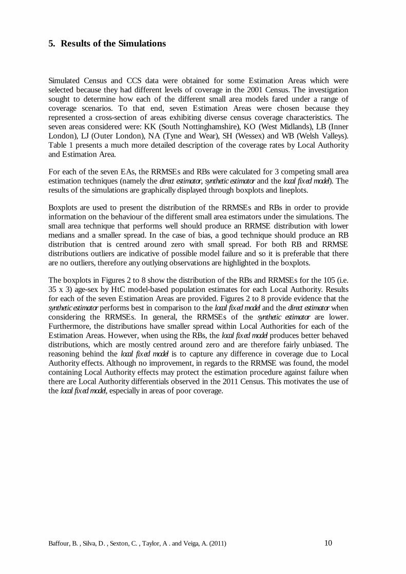
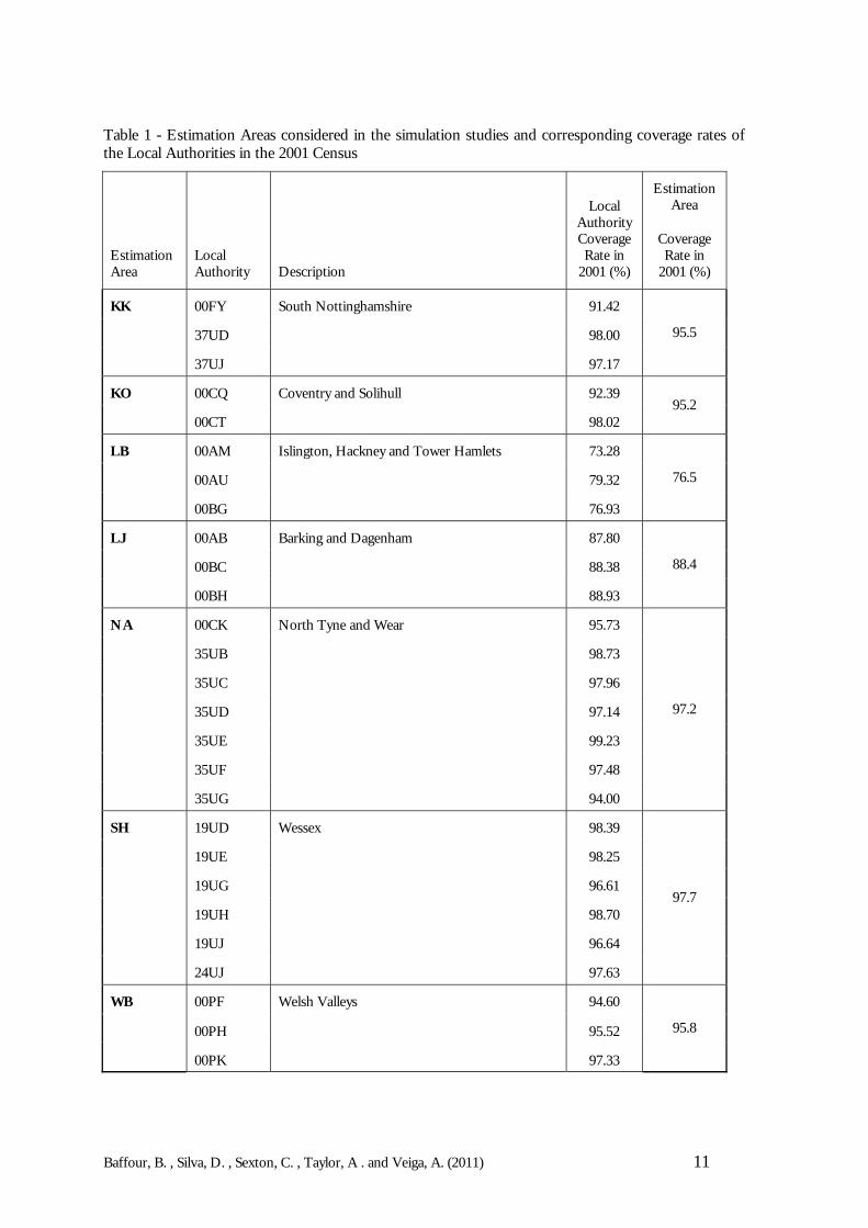
Simulated Census and CCS data were obtained for some Estimation Areas which wereselected because they had different levels of coverage in the 2001 Census. The investigationsought to determine how each of the different small area models fared under a range ofcoverage scenarios. To that end, seven Estimation Areas were chosen because theyrepresented a cross-section of areas exhibiting diverse census coverage characteristics. Theseven areas considered were: KK (South Nottinghamshire), KO (West Midlands), LB (InnerLondon), LJ (Outer London), NA (Tyne and Wear), SH (Wessex) and WB (Welsh Valleys).Table 1 presents a much more detailed description of the coverage rates by Local Authorityand Estimation Area.
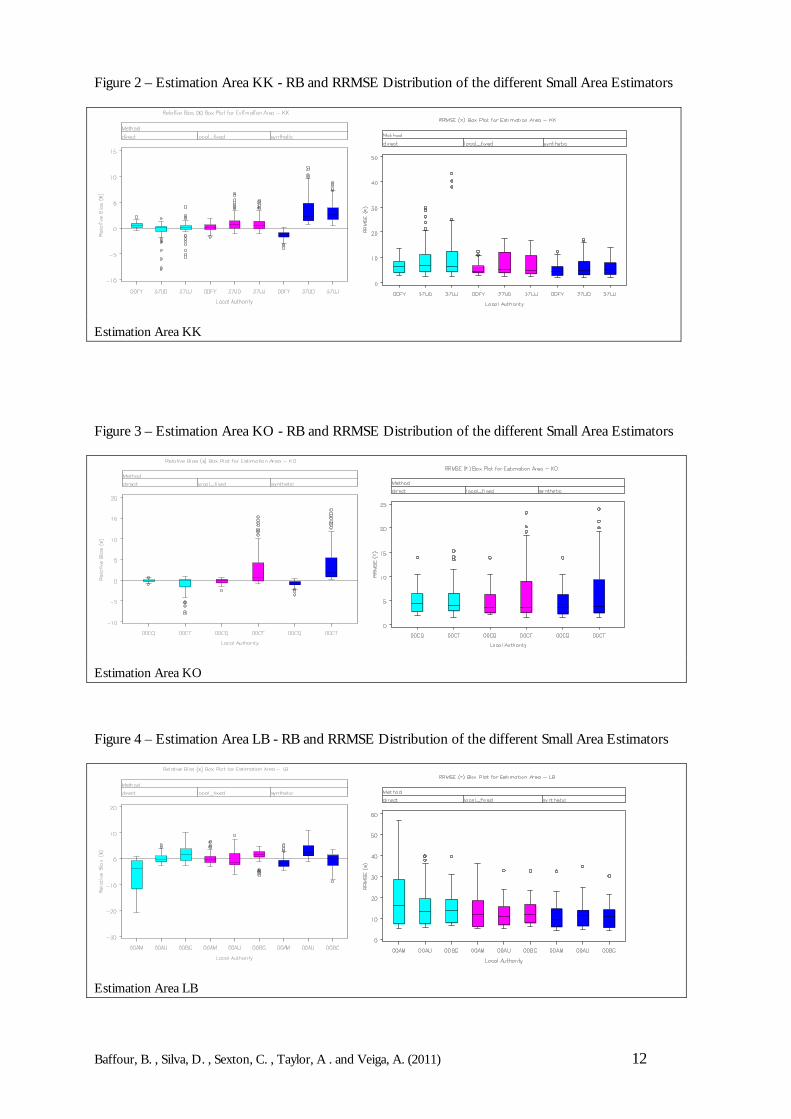
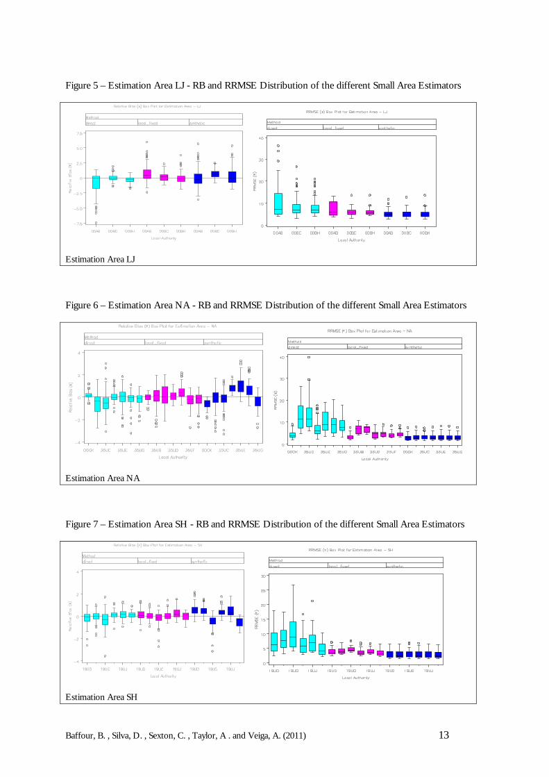
For each of the seven EAs, the RRMSEs and RBs were calculated for 3 competing small areaestimation techniques (namely the direct estimator, synthetic estimator and the local fixed model). Theresults of the simulations are graphically displayed through boxplots and lineplots.
Boxplots are used to present the distribution of the RRMSEs and RBs in order to provideinformation on the behaviour of the different small area estimators under the simulations. Thesmall area technique that performs well should produce an RRMSE distribution with lowermedians and a smaller spread. In the case of bias, a good technique should produce an RBdistribution that is centred around zero with small spread. For both RB and RRMSEdistributions outliers are indicative of possible model failure and so it is preferable that thereare no outliers, therefore any outlying observations are highlighted in the boxplots.
The boxplots in Figures 2 to 8 show the distribution of the RBs and RRMSEs for the 105 (i.e.35 x 3) age-sex by HtC model-based population estimates for each Local Authority. Resultsfor each of the seven Estimation Areas are provided. Figures 2 to 8 provide evidence that thesynthetic estimator performs best in comparison to the local fixed model and the direct estimator whenconsidering the RRMSEs. In general, the RRMSEs of the synthetic estimator are lower.Furthermore, the distributions have smaller spread within Local Authorities for each of theEstimation Areas. However, when using the RBs, the local fixed model produces better behaveddistributions, which are mostly centred around zero and are therefore fairly unbiased. Thereasoning behind the local fixed model is to capture any difference in coverage due to LocalAuthority effects. Although no improvement, in regards to the RRMSE was found, the modelcontaining Local Authority effects may protect the estimation procedure against failure whenthere are Local Authority differentials observed in the 2011 Census. This motivates the use ofthe local fixed model, especially in areas of poor coverage.
Baffour, B. , Silva, D. , Sexton, C. , Taylor, A . and Veiga, A. (2011) 11
Table 1 - Estimation Areas considered in the simulation studies and corresponding coverage rates ofthe Local Authorities in the 2001 Census
EstimationArea
LocalAuthority Description
LocalAuthorityCoverageRate in
2001 (%)
EstimationArea
CoverageRate in
2001 (%)
KK 00FY South Nottinghamshire 91.42
37UD 98.00
37UJ 97.17
95.5
KO 00CQ Coventry and Solihull 92.39
00CT 98.0295.2
LB 00AM Islington, Hackney and Tower Hamlets 73.28
00AU 79.32
00BG 76.93
76.5
LJ 00AB Barking and Dagenham 87.80
00BC 88.38
00BH 88.93
88.4
NA 00CK North Tyne and Wear 95.73
35UB 98.73
35UC 97.96
35UD 97.14
35UE 99.23
35UF 97.48
35UG 94.00
97.2
SH 19UD Wessex 98.39
19UE 98.25
19UG 96.61
19UH 98.70
19UJ 96.64
24UJ 97.63
97.7
WB 00PF Welsh Valleys 94.60
00PH 95.52
00PK 97.33
95.8
Baffour, B. , Silva, D. , Sexton, C. , Taylor, A . and Veiga, A. (2011) 12
Figure 2 – Estimation Area KK - RB and RRMSE Distribution of the different Small Area Estimators
Estimation Area KK
Figure 3 – Estimation Area KO - RB and RRMSE Distribution of the different Small Area Estimators
Estimation Area KO
Figure 4 – Estimation Area LB - RB and RRMSE Distribution of the different Small Area Estimators
Estimation Area LB
Baffour, B. , Silva, D. , Sexton, C. , Taylor, A . and Veiga, A. (2011) 13
Figure 5 – Estimation Area LJ - RB and RRMSE Distribution of the different Small Area Estimators
Estimation Area LJ
Figure 6 – Estimation Area NA - RB and RRMSE Distribution of the different Small Area Estimators
Estimation Area NA
Figure 7 – Estimation Area SH - RB and RRMSE Distribution of the different Small Area Estimators
Estimation Area SH
Baffour, B. , Silva, D. , Sexton, C. , Taylor, A . and Veiga, A. (2011) 14
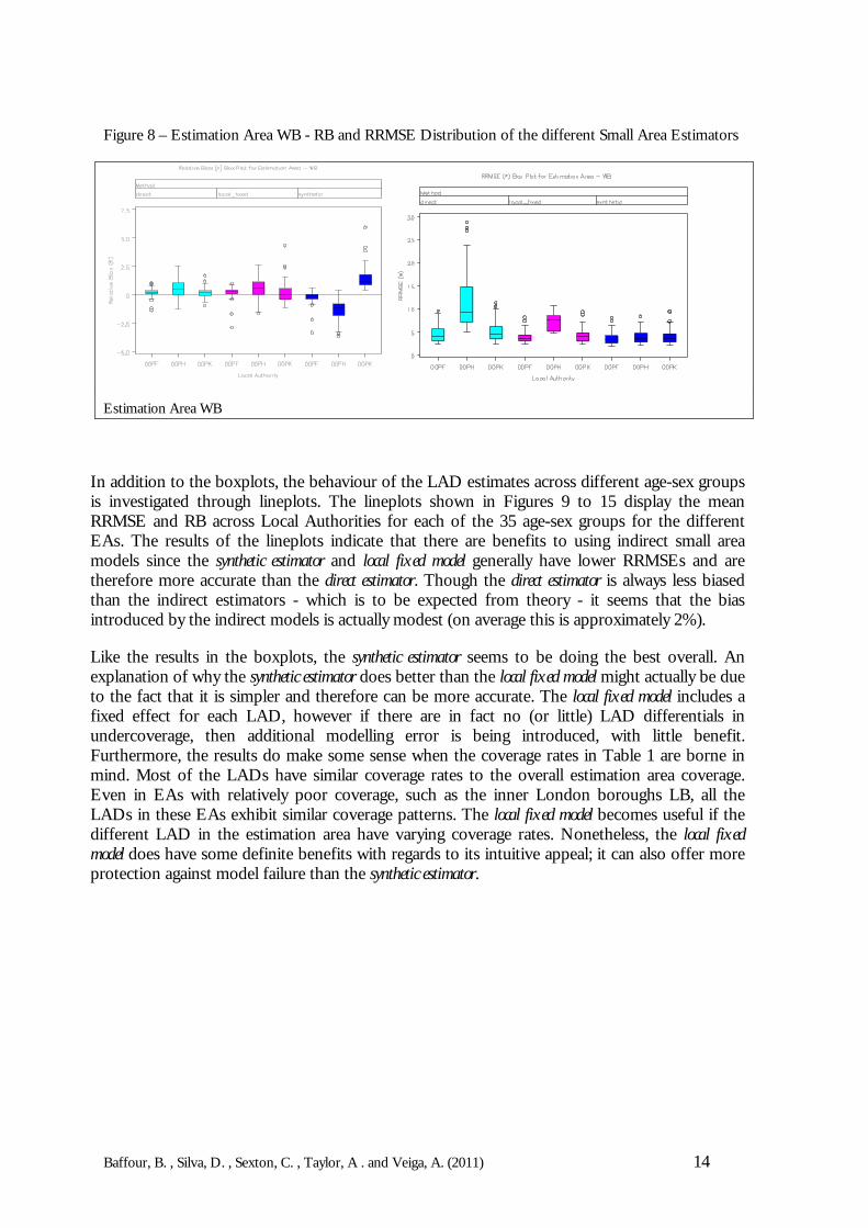
Figure 8 – Estimation Area WB - RB and RRMSE Distribution of the different Small Area Estimators
Estimation Area WB
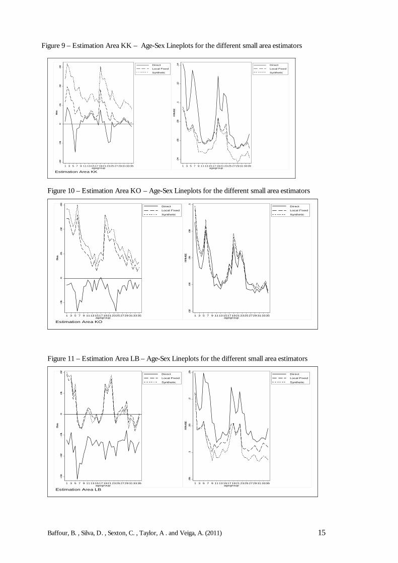
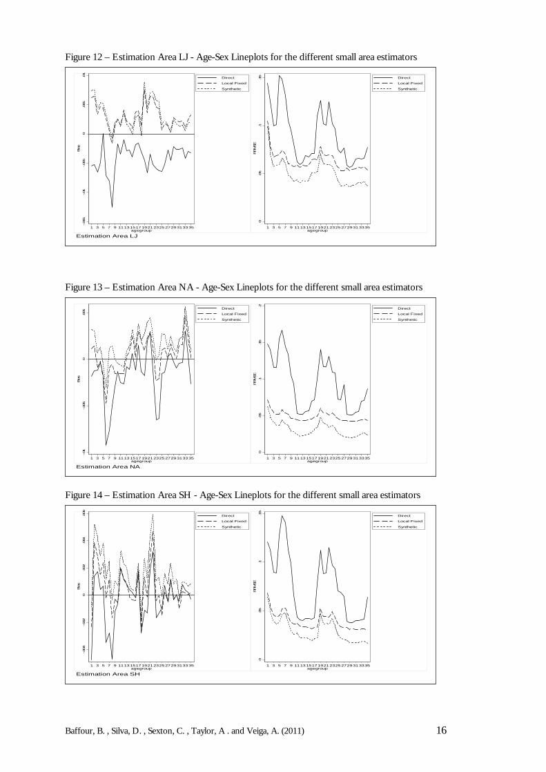
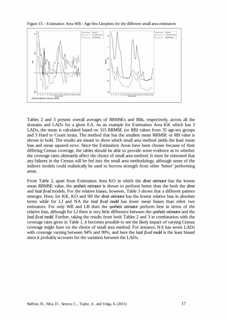
In addition to the boxplots, the behaviour of the LAD estimates across different age-sex groupsis investigated through lineplots. The lineplots shown in Figures 9 to 15 display the meanRRMSE and RB across Local Authorities for each of the 35 age-sex groups for the differentEAs. The results of the lineplots indicate that there are benefits to using indirect small areamodels since the synthetic estimator and local fixed model generally have lower RRMSEs and aretherefore more accurate than the direct estimator. Though the direct estimator is always less biasedthan the indirect estimators - which is to be expected from theory - it seems that the biasintroduced by the indirect models is actually modest (on average this is approximately 2%).
Like the results in the boxplots, the synthetic estimator seems to be doing the best overall. Anexplanation of why the synthetic estimator does better than the local fixed model might actually be dueto the fact that it is simpler and therefore can be more accurate. The local fixed model includes afixed effect for each LAD, however if there are in fact no (or little) LAD differentials inundercoverage, then additional modelling error is being introduced, with little benefit.Furthermore, the results do make some sense when the coverage rates in Table 1 are borne inmind. Most of the LADs have similar coverage rates to the overall estimation area coverage.Even in EAs with relatively poor coverage, such as the inner London boroughs LB, all theLADs in these EAs exhibit similar coverage patterns. The local fixed model becomes useful if thedifferent LAD in the estimation area have varying coverage rates. Nonetheless, the local fixedmodel does have some definite benefits with regards to its intuitive appeal; it can also offer moreprotection against model failure than the synthetic estimator.
Baffour, B. , Silva, D. , Sexton, C. , Taylor, A . and Veiga, A. (2011) 15
-.01
0.01
.02
.03
Bias
1 3 5 7 9 11131517192123252729313335agegroup
Direct
Local Fixed
Synthetic
.02
.04
.06
.08
.1RRM
SE
1 3 5 7 9 11131517192123252729313335agegroup
Direct
Local Fixed
Synthetic
Estimation Area KO
-.03
-.02
-.01
0.01
.02
Bias
1 3 5 7 9 11131517192123252729313335agegroup
Direct
Local Fixed
Synthetic
.05
.1.15
.2.25
RRM
SE
1 3 5 7 9 11131517192123252729313335agegroup
Direct
Local Fixed
Synthetic
Estimation Area LB
Figure 9 – Estimation Area KK – Age-Sex Lineplots for the different small area estimators
-.02
-.01
0.01
.02
.03
Bias
1 3 5 7 9 11131517192123252729313335agegroup
Direct
Local Fixed
Synthetic
.04
.06
.08
.1.12
.14
RRM
SE
1 3 5 7 9 11131517192123252729313335agegroup
Direct
Local Fixed
Synthetic
Estimation Area KK
Figure 10 – Estimation Area KO – Age-Sex Lineplots for the different small area estimators
Figure 11 – Estimation Area LB – Age-Sex Lineplots for the different small area estimators
Baffour, B. , Silva, D. , Sexton, C. , Taylor, A . and Veiga, A. (2011) 16
-.015
-.01
-.005
0.005
.01
Bias
1 3 5 7 9 11131517192123252729313335agegroup
Direct
Local Fixed
Synthetic
0.05
.1.15
RRM
SE
1 3 5 7 9 11131517192123252729313335agegroup
Direct
Local Fixed
Synthetic
Estimation Area LJ
-.01
-.005
0.005
Bias
1 3 5 7 9 11131517192123252729313335agegroup
Direct
Local Fixed
Synthetic
0.05
.1.15
.2RRM
SE
1 3 5 7 9 11131517192123252729313335agegroup
Direct
Local Fixed
Synthetic
Estimation Area NA
-.004
-.002
0.002
.004
.006
Bias
1 3 5 7 9 11131517192123252729313335agegroup
Direct
Local Fixed
Synthetic
0.05
.1.15
RRM
SE
1 3 5 7 9 11131517192123252729313335agegroup
Direct
Local Fixed
Synthetic
Estimation Area SH
Figure 12 – Estimation Area LJ - Age-Sex Lineplots for the different small area estimators
Figure 13 – Estimation Area NA - Age-Sex Lineplots for the different small area estimators
Figure 14 – Estimation Area SH - Age-Sex Lineplots for the different small area estimators
Baffour, B. , Silva, D. , Sexton, C. , Taylor, A . and Veiga, A. (2011) 17
-.005
0.005
.01
Bias
1 3 5 7 9 11131517192123252729313335agegroup
Direct
Local Fixed
Synthetic
.02
.04
.06
.08
.1.12
RRM
SE
1 3 5 7 9 11131517192123252729313335agegroup
Direct
Local Fixed
Synthetic
Estimation Area WB
Figure 15 – Estimation Area WB - Age-Sex Lineplots for the different small area estimators
Tables 2 and 3 present overall averages of RRMSEs and RBs, respectively, across all thedomains and LADs for a given EA. As an example for Estimation Area KK which has 3LADs, the mean is calculated based on 315 RRMSE (or RB) values from 35 age-sex groupsand 3 Hard to Count strata. The method that has the smallest mean RRMSE or RB value isshown in bold. The results are meant to show which small area method yields the least meanbias and mean squared error. Since the Estimation Areas have been chosen because of theirdiffering Census coverage, the tables should be able to provide some evidence as to whetherthe coverage rates ultimately affect the choice of small area method. It must be reiterated thatany failures in the Census will be fed into the small area methodology, although some of theindirect models could realistically be used to borrow strength from other ‘better’ performingareas.
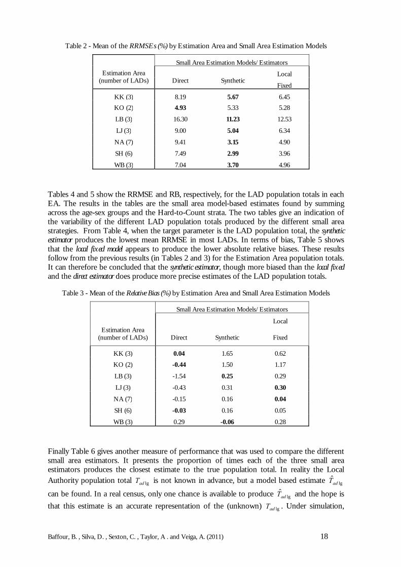
From Table 2, apart from Estimation Area KO in which the direct estimator has the lowestmean RRMSE value, the synthetic estimator is shown to perform better than the both the directand local fixed models. For the relative biases, however, Table 3 shows that a different patternemerges. Here, for KK, KO and SH the direct estimator has the lowest relative bias in absoluteterms while for LJ and NA the local fixed model has lower mean biases than other twoestimators. For only WB and LB does the synthetic estimator perform best in terms of therelative bias, although for LJ there is very little difference between the synthetic estimator and thelocal fixed model. Further, taking the results from both Tables 2 and 3 in combination with thecoverage rates given in Table 1, it becomes possible to see the likely impact of varying Censuscoverage might have on the choice of small area method. For instance, NA has seven LADswith coverage varying between 94% and 99%, and here the local fixed model is the least biasedsince it probably accounts for the variation between the LADs.
Baffour, B. , Silva, D. , Sexton, C. , Taylor, A . and Veiga, A. (2011) 18
Table 2 - Mean of the RRMSEs (%) by Estimation Area and Small Area Estimation Models
Small Area Estimation Models/Estimators
LocalEstimation Area(number of LADs) Direct Synthetic
Fixed
KK (3) 8.19 5.67 6.45KO (2) 4.93 5.33 5.28
LB (3) 16.30 11.23 12.53
LJ (3) 9.00 5.04 6.34
NA (7) 9.41 3.15 4.90
SH (6) 7.49 2.99 3.96
WB (3) 7.04 3.70 4.96
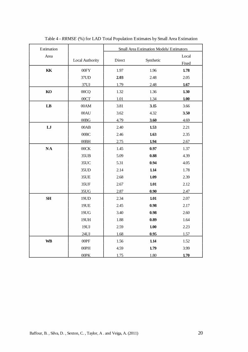
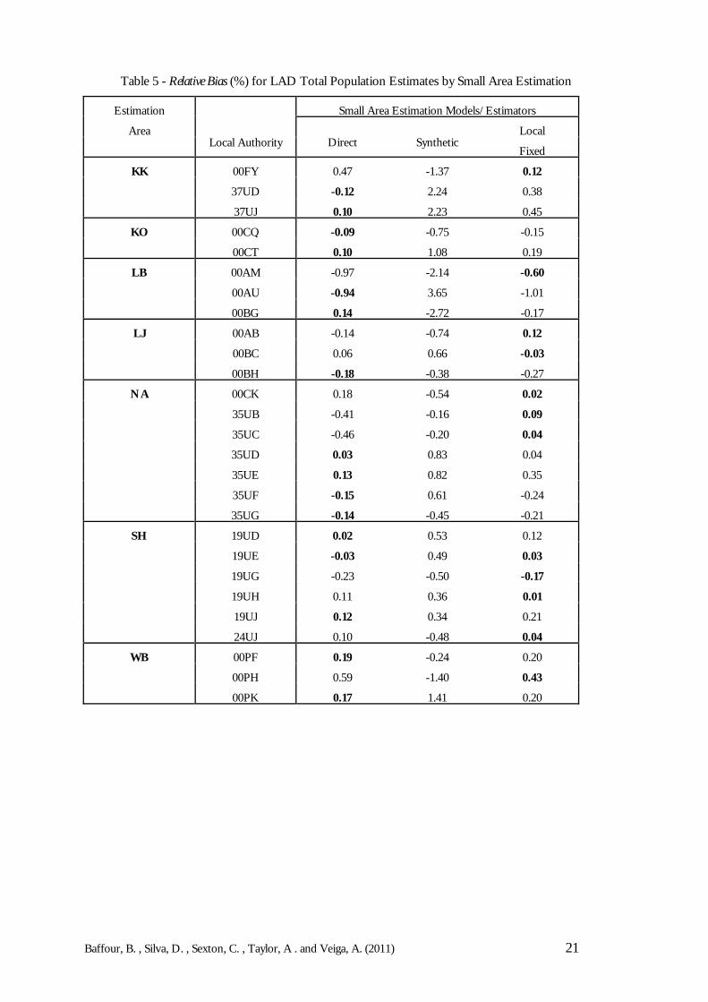
Tables 4 and 5 show the RRMSE and RB, respectively, for the LAD population totals in eachEA. The results in the tables are the small area model-based estimates found by summingacross the age-sex groups and the Hard-to-Count strata. The two tables give an indication ofthe variability of the different LAD population totals produced by the different small areastrategies. From Table 4, when the target parameter is the LAD population total, the syntheticestimator produces the lowest mean RRMSE in most LADs. In terms of bias, Table 5 showsthat the local fixed model appears to produce the lower absolute relative biases. These resultsfollow from the previous results (in Tables 2 and 3) for the Estimation Area population totals.It can therefore be concluded that the synthetic estimator, though more biased than the local fixedand the direct estimator does produce more precise estimates of the LAD population totals.
Table 3 - Mean of the Relative Bias (%) by Estimation Area and Small Area Estimation Models
Small Area Estimation Models/Estimators
LocalEstimation Area
(number of LADs) Direct Synthetic Fixed
KK (3) 0.04 1.65 0.62
KO (2) -0.44 1.50 1.17
LB (3) -1.54 0.25 0.29
LJ (3) -0.43 0.31 0.30
NA (7) -0.15 0.16 0.04
SH (6) -0.03 0.16 0.05
WB (3) 0.29 -0.06 0.28
Finally Table 6 gives another measure of performance that was used to compare the differentsmall area estimators. It presents the proportion of times each of the three small areaestimators produces the closest estimate to the true population total. In reality the LocalAuthority population total lgadT is not known in advance, but a model based estimate lgadT
can be found. In a real census, only one chance is available to produce lgadT and the hope isthat this estimate is an accurate representation of the (unknown) lgadT . Under simulation,
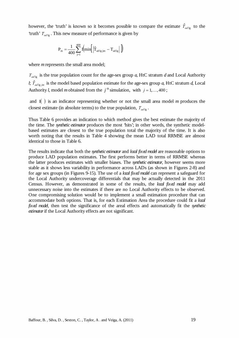
Baffour, B. , Silva, D. , Sexton, C. , Taylor, A . and Veiga, A. (2011) 19
however, the ‘truth’ is known so it becomes possible to compare the estimate lgadT to the‘truth’ lgadT . This new measure of performance is given by
[ ]( )∑=
−=400
1jlgadjmlgadm TT minI
4001P
where m represents the small area model;
lgadT is the true population count for the age-sex group a, HtC stratum d and Local Authority
l; jmadT lgˆ is the model based population estimate for the age-sex group a, HtC stratum d, Local
Authority l, model m obtained from the j th simulation, with 400,,1K=j ;
and ( )I is an indicator representing whether or not the small area model m produces theclosest estimate (in absolute terms) to the true population, lgadT .
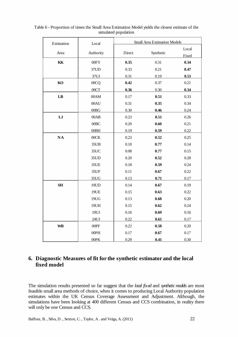
Thus Table 6 provides an indication to which method gives the best estimate the majority ofthe time. The synthetic estimator produces the most ‘hits’; in other words, the synthetic model-based estimates are closest to the true population total the majority of the time. It is alsoworth noting that the results in Table 4 showing the mean LAD total RRMSE are almostidentical to those in Table 6.
The results indicate that both the synthetic estimator and local fixed model are reasonable options toproduce LAD population estimates. The first performs better in terms of RRMSE whereasthe latter produces estimates with smaller biases. The synthetic estimator, however seems morestable as it shows less variability in performance across LADs (as shown in Figures 2-8) andfor age sex groups (in Figures 9-15). The use of a local fixed model can represent a safeguard forthe Local Authority undercoverage differentials that may be actually detected in the 2011Census. However, as demonstrated in some of the results, the local fixed model may addunnecessary noise into the estimates if there are no Local Authority effects to be observed.One compromising solution would be to implement a small estimation procedure that canaccommodate both options. That is, for each Estimation Area the procedure could fit a localfixed model, then test the significance of the areal effects and automatically fit the syntheticestimator if the Local Authority effects are not significant.
Baffour, B. , Silva, D. , Sexton, C. , Taylor, A . and Veiga, A. (2011) 20
Table 4 - RRMSE (%) for LAD Total Population Estimates by Small Area Estimation
Estimation Small Area Estimation Models/Estimators
Area Local
Local Authority Direct Synthetic
Fixed
00FY 1.97 1.96 1.78
37UD 2.03 2.48 2.05
KK
37UJ 1.79 2.48 1.67
00CQ 1.32 1.36 1.30KO
00CT 1.01 1.34 1.00
00AM 3.81 3.15 3.66
00AU 3.62 4.32 3.50
LB
00BG 4.79 3.60 4.69
00AB 2.40 1.53 2.21
00BC 2.46 1.63 2.35
LJ
00BH 2.75 1.94 2.67
00CK 1.45 0.97 1.37
35UB 5.09 0.88 4.39
35UC 5.31 0.94 4.05
35UD 2.14 1.14 1.78
35UE 2.68 1.09 2.39
35UF 2.67 1.01 2.12
NA
35UG 2.87 0.90 2.47
19UD 2.34 1.01 2.07
19UE 2.45 0.98 2.17
19UG 3.40 0.98 2.60
19UH 1.88 0.89 1.64
19UJ 2.59 1.00 2.23
SH
24UJ 1.68 0.95 1.57
00PF 1.56 1.14 1.52
00PH 4.59 1.79 3.99
WB
00PK 1.75 1.80 1.70
Baffour, B. , Silva, D. , Sexton, C. , Taylor, A . and Veiga, A. (2011) 21
Table 5 - Relative Bias (%) for LAD Total Population Estimates by Small Area Estimation
Estimation Small Area Estimation Models/Estimators
Area Local
Local Authority Direct Synthetic
Fixed
00FY 0.47 -1.37 0.12
37UD -0.12 2.24 0.38
KK
37UJ 0.10 2.23 0.45
00CQ -0.09 -0.75 -0.15KO
00CT 0.10 1.08 0.19
00AM -0.97 -2.14 -0.60
00AU -0.94 3.65 -1.01
LB
00BG 0.14 -2.72 -0.17
00AB -0.14 -0.74 0.12
00BC 0.06 0.66 -0.03
LJ
00BH -0.18 -0.38 -0.27
00CK 0.18 -0.54 0.02
35UB -0.41 -0.16 0.09
35UC -0.46 -0.20 0.04
35UD 0.03 0.83 0.04
35UE 0.13 0.82 0.35
35UF -0.15 0.61 -0.24
NA
35UG -0.14 -0.45 -0.21
19UD 0.02 0.53 0.12
19UE -0.03 0.49 0.03
19UG -0.23 -0.50 -0.17
19UH 0.11 0.36 0.01
19UJ 0.12 0.34 0.21
SH
24UJ 0.10 -0.48 0.04
00PF 0.19 -0.24 0.20
00PH 0.59 -1.40 0.43
WB
00PK 0.17 1.41 0.20
Baffour, B. , Silva, D. , Sexton, C. , Taylor, A . and Veiga, A. (2011) 22
Table 6 - Proportion of times the Small Area Estimation Model yields the closest estimate of thesimulated population
Small Area Estimation Models
LocalEstimation
Area
Local
Authority Direct SyntheticFixed
00FY 0.35 0.31 0.34
37UD 0.33 0.21 0.47
KK
37UJ 0.31 0.19 0.51
00CQ 0.42 0.37 0.21KO
00CT 0.36 0.30 0.34
00AM 0.17 0.51 0.33
00AU 0.31 0.35 0.34
LB
00BG 0.30 0.46 0.24
00AB 0.23 0.51 0.26
00BC 0.20 0.60 0.21
LJ
00BH 0.19 0.59 0.22
00CK 0.23 0.52 0.25
35UB 0.10 0.77 0.14
35UC 0.08 0.77 0.15
35UD 0.20 0.52 0.28
35UE 0.18 0.59 0.24
35UF 0.11 0.67 0.22
NA
35UG 0.13 0.71 0.17
19UD 0.14 0.67 0.19
19UE 0.15 0.63 0.22
19UG 0.13 0.68 0.20
19UH 0.15 0.62 0.24
19UJ 0.16 0.69 0.16
SH
24UJ 0.22 0.61 0.17
00PF 0.22 0.58 0.20
00PH 0.17 0.67 0.17
WB
00PK 0.29 0.41 0.30
6. Diagnostic Measures of fit for the synthetic estimator and the localfixed model
The simulation results presented so far suggest that the local fixed and synthetic models are mostfeasible small area methods of choice, when it comes to producing Local Authority populationestimates within the UK Census Coverage Assessment and Adjustment. Although, thesimulations have been looking at 400 different Census and CCS combination, in reality therewill only be one Census and CCS.
Baffour, B. , Silva, D. , Sexton, C. , Taylor, A . and Veiga, A. (2011) 23
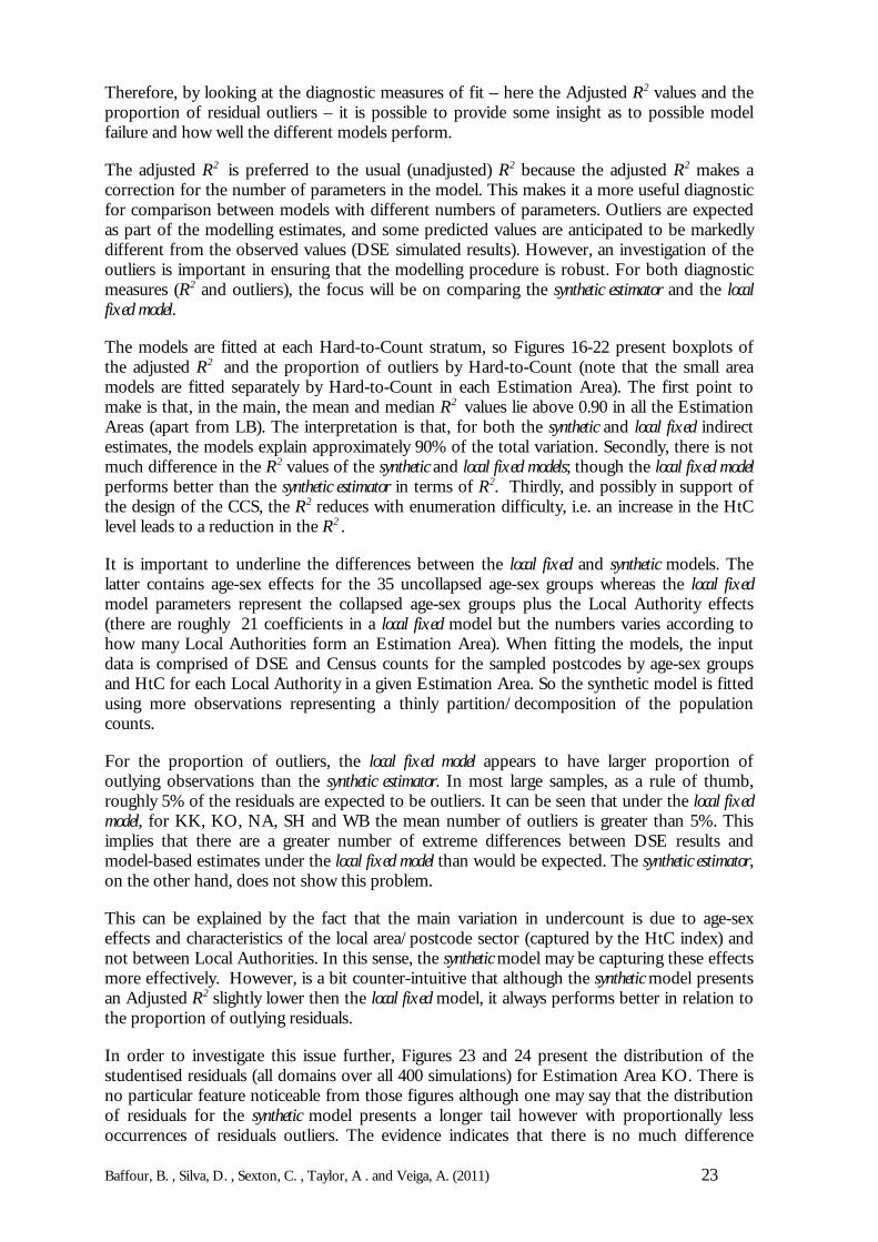
Therefore, by looking at the diagnostic measures of fit – here the Adjusted R2 values and theproportion of residual outliers – it is possible to provide some insight as to possible modelfailure and how well the different models perform.
The adjusted R2 is preferred to the usual (unadjusted) R2 because the adjusted R2 makes acorrection for the number of parameters in the model. This makes it a more useful diagnosticfor comparison between models with different numbers of parameters. Outliers are expectedas part of the modelling estimates, and some predicted values are anticipated to be markedlydifferent from the observed values (DSE simulated results). However, an investigation of theoutliers is important in ensuring that the modelling procedure is robust. For both diagnosticmeasures (R2 and outliers), the focus will be on comparing the synthetic estimator and the localfixed model.
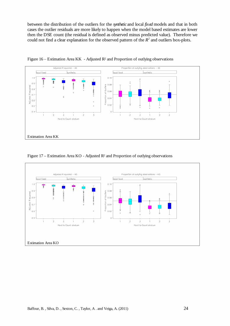
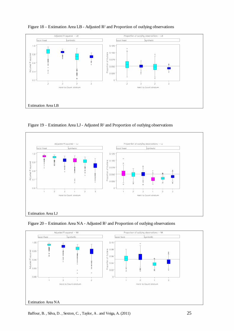
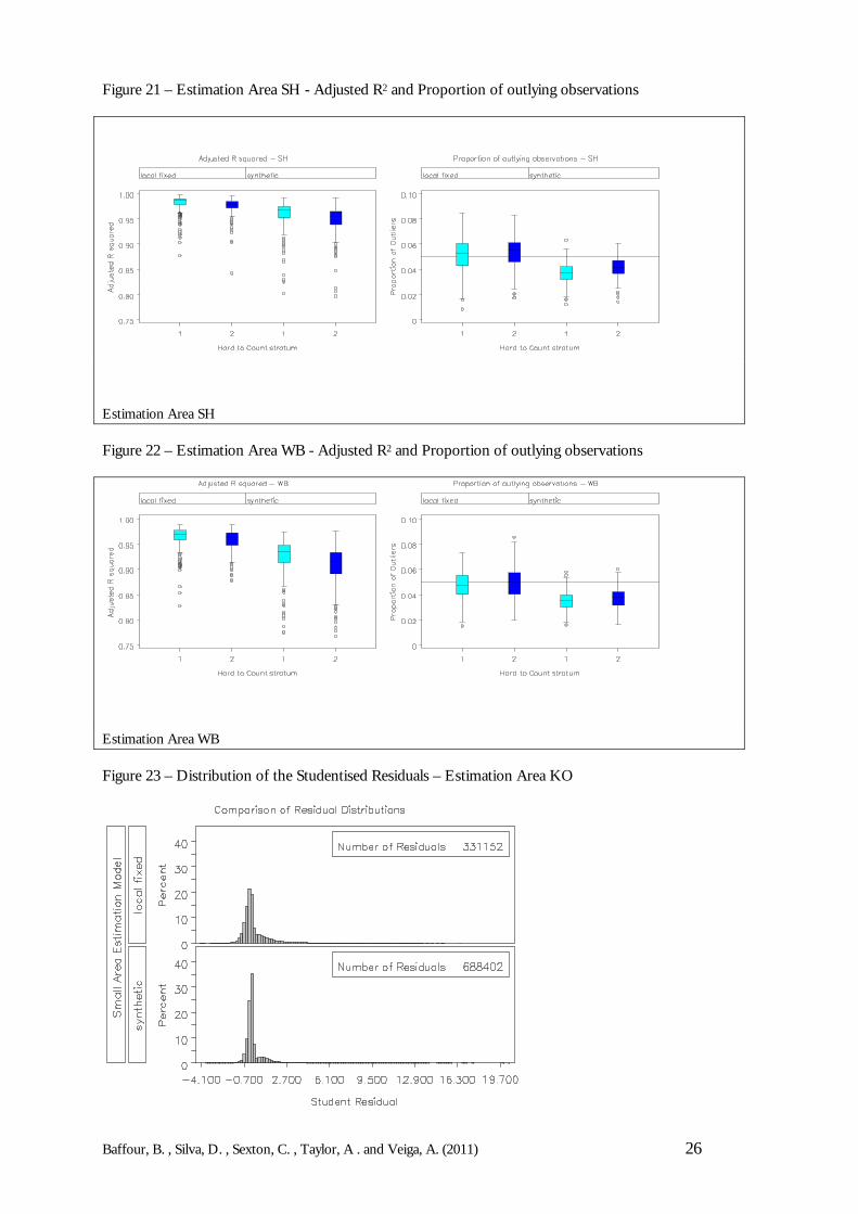
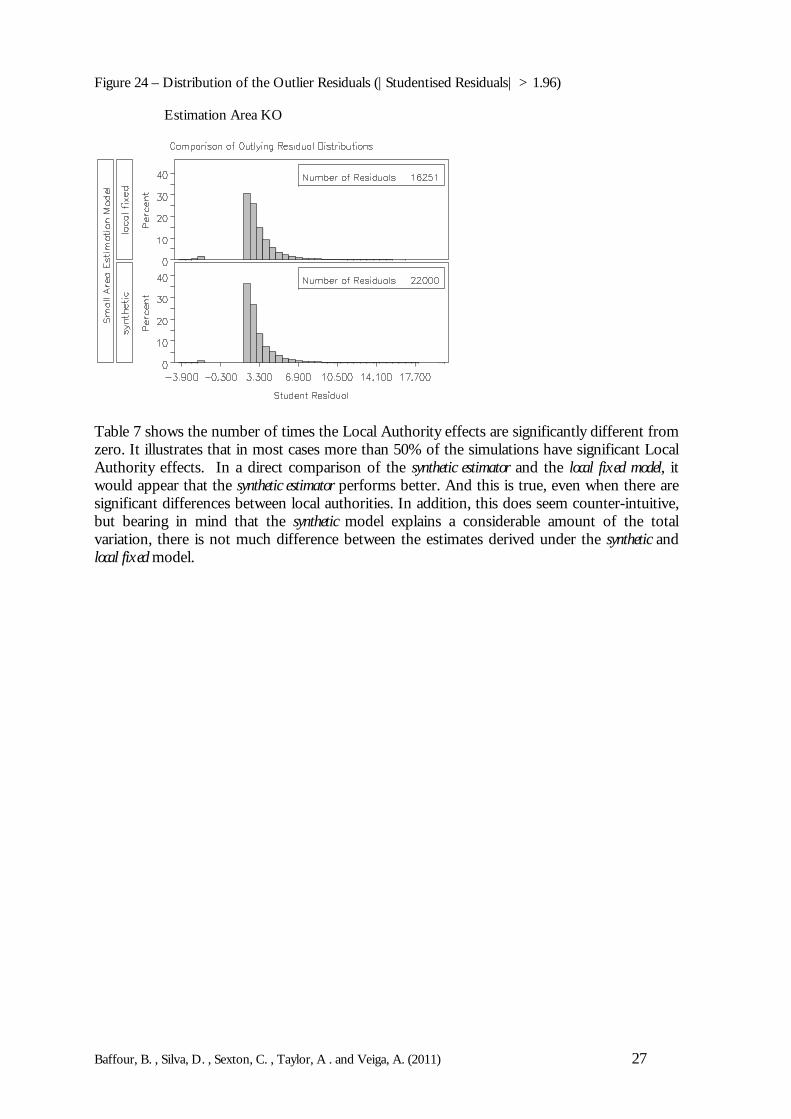
The models are fitted at each Hard-to-Count stratum, so Figures 16-22 present boxplots ofthe adjusted R2 and the proportion of outliers by Hard-to-Count (note that the small areamodels are fitted separately by Hard-to-Count in each Estimation Area). The first point tomake is that, in the main, the mean and median R2 values lie above 0.90 in all the EstimationAreas (apart from LB). The interpretation is that, for both the synthetic and local fixed indirectestimates, the models explain approximately 90% of the total variation. Secondly, there is notmuch difference in the R2 values of the synthetic and local fixed models; though the local fixed modelperforms better than the synthetic estimator in terms of R2. Thirdly, and possibly in support ofthe design of the CCS, the R2 reduces with enumeration difficulty, i.e. an increase in the HtClevel leads to a reduction in the R2 .
It is important to underline the differences between the local fixed and synthetic models. Thelatter contains age-sex effects for the 35 uncollapsed age-sex groups whereas the local fixedmodel parameters represent the collapsed age-sex groups plus the Local Authority effects(there are roughly 21 coefficients in a local fixed model but the numbers varies according tohow many Local Authorities form an Estimation Area). When fitting the models, the inputdata is comprised of DSE and Census counts for the sampled postcodes by age-sex groupsand HtC for each Local Authority in a given Estimation Area. So the synthetic model is fittedusing more observations representing a thinly partition/decomposition of the populationcounts.
For the proportion of outliers, the local fixed model appears to have larger proportion ofoutlying observations than the synthetic estimator. In most large samples, as a rule of thumb,roughly 5% of the residuals are expected to be outliers. It can be seen that under the local fixedmodel, for KK, KO, NA, SH and WB the mean number of outliers is greater than 5%. Thisimplies that there are a greater number of extreme differences between DSE results andmodel-based estimates under the local fixed model than would be expected. The synthetic estimator,on the other hand, does not show this problem.
This can be explained by the fact that the main variation in undercount is due to age-sexeffects and characteristics of the local area/postcode sector (captured by the HtC index) andnot between Local Authorities. In this sense, the synthetic model may be capturing these effectsmore effectively. However, is a bit counter-intuitive that although the synthetic model presentsan Adjusted R2 slightly lower then the local fixed model, it always performs better in relation tothe proportion of outlying residuals.
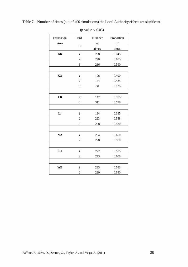
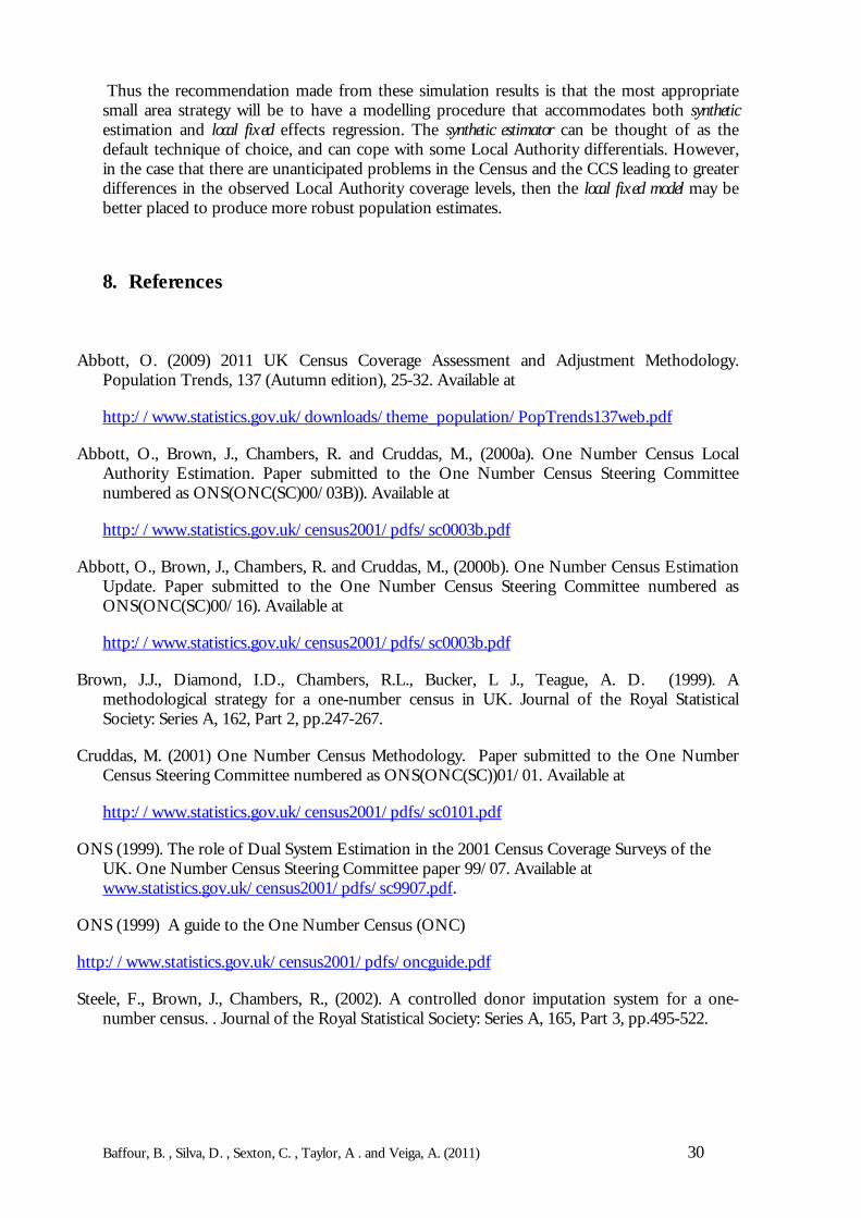
In order to investigate this issue further, Figures 23 and 24 present the distribution of thestudentised residuals (all domains over all 400 simulations) for Estimation Area KO. There isno particular feature noticeable from those figures although one may say that the distributionof residuals for the synthetic model presents a longer tail however with proportionally lessoccurrences of residuals outliers. The evidence indicates that there is no much difference
Baffour, B. , Silva, D. , Sexton, C. , Taylor, A . and Veiga, A. (2011) 24
between the distribution of the outliers for the synthetic and local fixed models and that in bothcases the outlier residuals are more likely to happen when the model based estimates are lowerthen the DSE count (the residual is defined as observed minus predicted value). Therefore wecould not find a clear explanation for the observed pattern of the R2 and outliers box-plots.
Figure 16 – Estimation Area KK - Adjusted R2 and Proportion of outlying observations
Estimation Area KK
Figure 17 – Estimation Area KO - Adjusted R2 and Proportion of outlying observations
Estimation Area KO
Baffour, B. , Silva, D. , Sexton, C. , Taylor, A . and Veiga, A. (2011) 25
Figure 18 – Estimation Area LB - Adjusted R2 and Proportion of outlying observations
Estimation Area LB
Figure 19 – Estimation Area LJ - Adjusted R2 and Proportion of outlying observations
Estimation Area LJ
Figure 20 – Estimation Area NA - Adjusted R2 and Proportion of outlying observations
Estimation Area NA
Baffour, B. , Silva, D. , Sexton, C. , Taylor, A . and Veiga, A. (2011) 26
Figure 21 – Estimation Area SH - Adjusted R2 and Proportion of outlying observations
Estimation Area SH
Figure 22 – Estimation Area WB - Adjusted R2 and Proportion of outlying observations
Estimation Area WB
Figure 23 – Distribution of the Studentised Residuals – Estimation Area KO
Baffour, B. , Silva, D. , Sexton, C. , Taylor, A . and Veiga, A. (2011) 27
Figure 24 – Distribution of the Outlier Residuals (|Studentised Residuals| > 1.96)
Estimation Area KO
Table 7 shows the number of times the Local Authority effects are significantly different fromzero. It illustrates that in most cases more than 50% of the simulations have significant LocalAuthority effects. In a direct comparison of the synthetic estimator and the local fixed model, itwould appear that the synthetic estimator performs better. And this is true, even when there aresignificant differences between local authorities. In addition, this does seem counter-intuitive,but bearing in mind that the synthetic model explains a considerable amount of the totalvariation, there is not much difference between the estimates derived under the synthetic andlocal fixed model.
Baffour, B. , Silva, D. , Sexton, C. , Taylor, A . and Veiga, A. (2011) 28
Table 7 – Number of times (out of 400 simulations) the Local Authority effects are significant
(p-value < 0.05)
Estimation Number Proportion
Area of of
Hard
totimes times
KK 1 298 0.745 2 270 0.675
3 236 0.590
KO 1 196 0.490 2 174 0.435
3 50 0.125
LB 2 142 0.355 3 311 0.778
LJ 1 134 0.335 2 223 0.558
3 208 0.520
NA 1 264 0.660 2 228 0.570
SH 1 222 0.555 2 243 0.608
WB 1 233 0.583 2 220 0.550

Baffour, B. , Silva, D. , Sexton, C. , Taylor, A . and Veiga, A. (2011) 29
7. Conclusions
Small area estimation techniques are useful in overcoming the problem of small sample sizessince direct estimates using data from CCS will have correspondingly large standard errors andwill be imprecise. However, albeit precise, these model based estimators may be more biasedthan the direct estimators. Therefore, the aim of the evaluation of different estimators was tobalance the trade-off between variance and bias, in order to find the estimator that producesestimates with good precision and as little bias as possible. The small area models work byincorporating auxiliary information via assuming relationships between the undercount patternin the Local Authority and broader areas such as the Estimation Area. The underlying idearelies on exploiting the similarities in the undercount patterns so as to borrow strength overthe areas through the use of regression models relating the CCS counts to the Census counts.
It is clear that the small area estimation strategy is completely reliant on the CCS design andthe coverage assessment and adjustment processes used to obtain Estimation Area populationtotals. In 2001, the small area strategy was to produce model-based Local Authority estimatesby Hard-to-Count strata and age-sex groups. The model used was a simple linear regressionmodel using the CCS count as the response variable and the Census count as the explanatoryvariable, with different slope coefficients for each Local Authority within a chosen EstimationArea, in addition to an overall age-sex effect. These were then calibrated to the EstimationArea population totals.
One of the lessons learnt in the 2001 Census was that any shortcomings of the censusenumeration process will have an effect in the application of the small area methodology. Thiswill be much more apparent if direct estimation is used to produce Local Authority estimatesfrom the Estimation Area totals derived in the earlier census coverage adjustment processes.However, the indirect models such as the synthetic estimator, local fixed model and the regional fixedand mixed models can realistically be used to improve the precision of the Local Authorityestimates.
This improvement in precision is wholly dependent on being able to exploit the similaritiesbetween Local Authorities either within the Estimation Area or within the region. In thesimulation exercise, it has been demonstrated that the choice of the indirect model can becomplicated because it is often not easy to know how to exploit these similarities. Generallyspeaking, the Local Authorities within an Estimation Area are broadly similar; as such thesynthetic estimator will often be the most appropriate indirect model. The reason for this couldbe attributed to the design of the CCS in that the broad stratification of the UK intoEstimation Areas appropriately groups similar Local Authorities together. However, whenthere is localised failure of the Census (and/or CCS) - for example, a specific Local Authoritybehaves differently to the Estimation Area within which it is found - then the synthetic estimatorcan be less precise than the local fixed model.
When it is required to choose between the synthetic estimator and the local fixed model, themodel diagnostics show that the synthetic estimator performs better than the local fixed. Bothmodels explain a substantial amount of the total variation, and so are appropriate small areastrategies. The simulations have shown that the difference in explained variation between thesynthetic and local fixed is not that large. The distribution of estimates produced by the syntheticestimator has a smaller spread. In addition, there are fewer outliers, unlike those producedunder local fixed modelling. The combined effect of these two diagnostic measures is to makethe synthetic estimator give more accurate population estimates. On the other hand, the ability ofthe local fixed model to cope with Local Authority differentials can be its strength particularlywhen there are unexpected outcomes.
Baffour, B. , Silva, D. , Sexton, C. , Taylor, A . and Veiga, A. (2011) 30
Thus the recommendation made from these simulation results is that the most appropriatesmall area strategy will be to have a modelling procedure that accommodates both syntheticestimation and local fixed effects regression. The synthetic estimator can be thought of as thedefault technique of choice, and can cope with some Local Authority differentials. However,in the case that there are unanticipated problems in the Census and the CCS leading to greaterdifferences in the observed Local Authority coverage levels, then the local fixed model may bebetter placed to produce more robust population estimates.
8. References
Abbott, O. (2009) 2011 UK Census Coverage Assessment and Adjustment Methodology.Population Trends, 137 (Autumn edition), 25-32. Available at
http://www.statistics.gov.uk/downloads/theme_population/PopTrends137web.pdf
Abbott, O., Brown, J., Chambers, R. and Cruddas, M., (2000a). One Number Census LocalAuthority Estimation. Paper submitted to the One Number Census Steering Committeenumbered as ONS(ONC(SC)00/03B)). Available at
http://www.statistics.gov.uk/census2001/pdfs/sc0003b.pdf
Abbott, O., Brown, J., Chambers, R. and Cruddas, M., (2000b). One Number Census EstimationUpdate. Paper submitted to the One Number Census Steering Committee numbered asONS(ONC(SC)00/16). Available at
http://www.statistics.gov.uk/census2001/pdfs/sc0003b.pdf
Brown, J.J., Diamond, I.D., Chambers, R.L., Bucker, L J., Teague, A. D. (1999). Amethodological strategy for a one-number census in UK. Journal of the Royal StatisticalSociety: Series A, 162, Part 2, pp.247-267.
Cruddas, M. (2001) One Number Census Methodology. Paper submitted to the One NumberCensus Steering Committee numbered as ONS(ONC(SC))01/01. Available at
http://www.statistics.gov.uk/census2001/pdfs/sc0101.pdf
ONS (1999). The role of Dual System Estimation in the 2001 Census Coverage Surveys of theUK. One Number Census Steering Committee paper 99/07. Available atwww.statistics.gov.uk/census2001/pdfs/sc9907.pdf.
ONS (1999) A guide to the One Number Census (ONC)
http://www.statistics.gov.uk/census2001/pdfs/oncguide.pdf
Steele, F., Brown, J., Chambers, R., (2002). A controlled donor imputation system for a one-number census. . Journal of the Royal Statistical Society: Series A, 165, Part 3, pp.495-522.