Citation: Cucuzza, R.; Rosso, M.M.;

Aloisio, A.; Melchiorre, J.; Lo Giudice,

M.; Marano, G.C. Size and Shape

Optimization of a Guyed Mast

Structure under Wind, Ice and

Seismic Loading. Appl. Sci. 2022, 12,

4875. https://doi.org/10.3390/

app12104875

Academic Editors: Nikos D. Lagaros

and Vagelis Plevris

Received: 17 April 2022

Accepted: 9 May 2022

Published: 11 May 2022

Publisher’s Note: MDPI stays neutral

with regard to jurisdictional claims in

published maps and institutional affil-

iations.

Copyright: © 2022 by the authors.

Licensee MDPI, Basel, Switzerland.

This article is an open access article

distributed under the terms and

conditions of the Creative Commons

Attribution (CC BY) license (https://

creativecommons.org/licenses/by/

4.0/).

applied sciences

Article

Size and Shape Optimization of a Guyed Mast Structure underWind, Ice and Seismic Loading

Raffaele Cucuzza 1 , Marco Martino Rosso 1 , Angelo Aloisio 2,* , Jonathan Melchiorre 1 , Mario Lo Giudice 1

and Giuseppe Carlo Marano 1

1 Department of Structural, Geotechnical and Building Engineering, Politecnico di Torino,Corso Duca Degli Abruzzi, 24, 10128 Turin, Italy; raffaele.cucuzza@polito.it (R.C.);marco.rosso@polito.it (M.M.R.); jonathan.melchiorre@polito.it (J.M.); logiudice.mario@polito.it (M.L.G.);giuseppe.marano@polito.it (G.C.M.)

2 Civil Environmental and Architectural Engineering Department, Università Degli Studi dell’Aquila,via Giovanni Gronchi n.18, 67100 L’Aquila, Italy

* Correspondence: angelo.aloisio1@univaq.it

Abstract: This paper discusses the size and shape optimization of a guyed radio mast for radio-communications. The considered structure represents a widely industrial solution due to the recentspread of 5G and 6G mobile networks. The guyed radio mast was modeled with the finite elementsoftware SAP2000 and optimized through a genetic optimization algorithm (GA). The optimizationexploits the open application programming interfaces (OAPI) SAP2000-Matlab. Static and dynamicanalyses were carried out to provide realistic design scenarios of the mast structure. The authorsconsidered the action of wind, ice, and seismic loads as variable loads. A parametric study on themost critical design variables includes several optimization scenarios to minimize the structure’s totalself-weight by varying the most relevant parameters selected by a preliminary sensitivity analysis. Inconclusion, final design considerations are discussed by highlighting the best optimization scenarioin terms of the objective function and the number of parameters involved in the analysis.

Keywords: guyed mast; structural optimization; genetic algorithm; structural design

1. Introduction

Guyed masts are extensively used in the telecommunications industry, and thesize, shape, and topology optimization can significantly benefit their transportation andinstallation. The main loads acting on guyed mast structures arise from wind [1,2],earthquakes [3–6], sudden rupture of guys [7], galloping of guys [8], and sudden iceshedding from ice-laden guy wires [9].

Their optimization must fulfil several requirements under ultimate and service limitstates [10]. Specifically, service limit states are crucial for guyed mast structures due to high-amplitude oscillations caused by their high deformability. In some cases, these vibrationshave led to a signal loss caused by excessive displacement and rotation of the antennasand, in other cases, have resulted in permanent deformation or failure. Therefore, sizeoptimization of the guyed mast structure represents a challenging task since the incrementof the performance ratio of the materials should be counterbalanced by an adequate lateralstiffness to reduce high-vibration drawbacks [11].

Saxena [12] reported several happenings where heavy icing combined with moderatewind resulted in severe misalignment of towers and complete failure. Novak et al. [13]showed that ice accumulation on some parts of the guy wires and moderate winds couldlead to the guy galloping, resulting in unacceptable stress levels throughout the structure.The main topics investigated in the field of guyed structures can be summarized as follows:

• Structural design. Several researchers investigated the dynamic response of guyedmast structures through experimental tests and numerical modeling to derive design

Appl. Sci. 2022, 12, 4875. https://doi.org/10.3390/app12104875 https://www.mdpi.com/journal/applsci

Appl. Sci. 2022, 12, 4875 2 of 32

approaches and recommendations [14–16]. In particular, there are studies dealingwith the dynamic identification and accurate estimate of the wind loads [17–21].

• Nonlinear dynamics. The proneness to global and local instabilities challenged severalscholars to estimate and predict the nonlinear behaviour of guyed masts [22–26].

• Structural optimization. The need for guyed structures that are easy to install andtransport challenged several scholars to optimize their shape in order to reducethe structural mass without reducing the lateral stiffness and prevent instabilityphenomena [27].

• Structural control. There are some attempts of control methods to reduce vibrationsin mast-like structures [28–30]. Among others, Blachowski [31] proposed the use of ahydraulic actuator to control cable forces in guyed masts using Kalman filtering.

This paper tackles the size and shape optimization of guyed mast structures. A videoof the considered structure is available in Supplementary Material. Since the first attemptsby Bell and Brown [32], many engineers attempted to optimize guyed masts under windloads using deterministic global optimization algorithms. However, as pointed out by [27],this approach leads to local optimum points, since each design variable was consideredseparately. Thornton et al. [33] and Uys et al. [34] proposed general procedures foroptimizing steel towers under dynamic loads. To the author’s knowledge, Venanzi andMaterazzi [35] were the first to implement a multi-objective optimization method for guyedmast structures under wind loads using the stochastic simulated annealing algorithm forsize optimization. The objective function implemented by [35] included the sum of thesquares of the nodal displacements and the in-plan width of the structure. Zhang andLi [36] attempted to achieve both shape and size optimization in a two-step procedureusing the ant colony algorithm (ACA). Cucuzza et al. [37] proposed an alternative approachin which the multi-objective optimization problem has been reduced to a single-objectiveproblem through suitable parameters. Luh and Lin [38] were challenged in achievingthe topology, size, and shape optimization of guyed masts using a modification of thebinary particle swarm optimization (PSO) and the attractive and repulsive particle swarmoptimization.

This paper discusses the size optimization of guyed masts using a genetic algorithm (GA)by considering different design scenarios (e.g., Cucuzza et al. [37] and Manuello et al. [39]).Kaveh and Talatahari [40] noticed that the particle swarm optimization (PSO) is more effec-tive than ACA and the harmony search scheme for optimizing truss structures. However,Deng et al. [41] and Guo and Li [42] were successful in optimizing tapered masts andtransmission towers using modifications of genetic algorithms (GA). Moreover, Belevivciuset al. [27] attempted the topology-sizing optimization problem of the guyed mast as asingle-level single-objective global optimization problem using GAs.

Therefore, given the numerous successful solutions of guyed masts using GAs, theauthors chose to investigate the size optimization of a guyed mast structure using GAs. Fol-lowing [35], this paper focuses on the size optimization by considering eight possible designscenarios. The purpose of the present paper is two-fold. Firstly, this work aims at achievinga size optimization on a real application case adopting structural verification accordingto Eurocode 3. During the load evaluation phase, detailed analyses have been conducted,including wind, ice, and seismic actions and the verifications against instabilities. Secondly,the computational intelligence procedure adopted by the authors allowed the investigationof several scenarios simultaneously. As a result, the parameters that mainly affected thedesign process have been detected to provide preliminary indications to engineers in thepractical design of similar structural typologies. Furthermore, the considered case studymay represent a benchmark case for validating the reliability and accuracy of alternativenumerical approaches. Therefore, the paper is organized as follows. After the case studydescription and the FE model, the authors introduce the first numerical results and theoutcomes of the size and shape optimization.

Appl. Sci. 2022, 12, 4875 3 of 32

2. Case Study

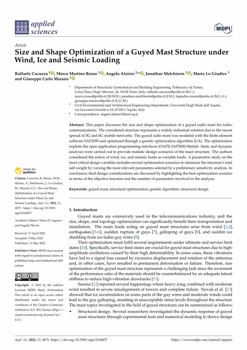
The considered structure is a guyed radio mast. It is a thin, slender, vertical structuresustained by tension cables fixed to the ground and typically arranged at 120° betweeneach other.

The main body is a single central column made of tube profiles or truss systems whena high elevation must be reached, see Figure 1. More than one set of cables is placed atdifferent elevations to prevent instability phenomena. Guyed towers are usually built formeteorological purposes or to support radio antennas, such as the one considered in thisresearch. In particular, this structure can be used for a limited time during an event ormaintenance of primary transmission towers. Therefore, it is also called a temporary basetransceiver station (BTS), typically adopted to supply the immediate service. Sportingevents, concerts, motor racing, military camps, and emergency events are typical examplesof temporary BTS applications. The BTS is usually mounted on a moveable platform calledthe shelter.

The considered structure is located in Bassano Del Grappa, in the north of Italy, ata 129 m elevation from the sea level. The surrounding area is low-urbanized, with norelevant obstacles to the wind loads. The total height of the mast is 30.00 m. It is sustainedby a central pole where 21 cables are fixed, see Figure 2. Other structural elements withrectangular cross-sections are used to create truss systems connecting cables and thecentral pole.

(a) (b)

Figure 1. (a) Render model realized using Tekla Structures. (b) Technical drawing of the structureinvestigated with dimensions in mm.

Appl. Sci. 2022, 12, 4875 4 of 32

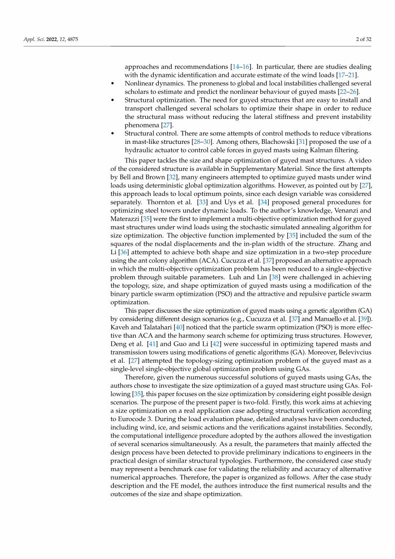
The central pole consists of five circular hollow steel profiles with flanged joints and6 m in length. All connections are bolted, as well as those connecting the cables to the pole.The shelter is a steel box devoted to partially sustaining the structure and hosting electronicequipment. It is usually mounted on a moveable platform.

Figure 2. Pictures and details of the considered structure.

3. Load Analysis

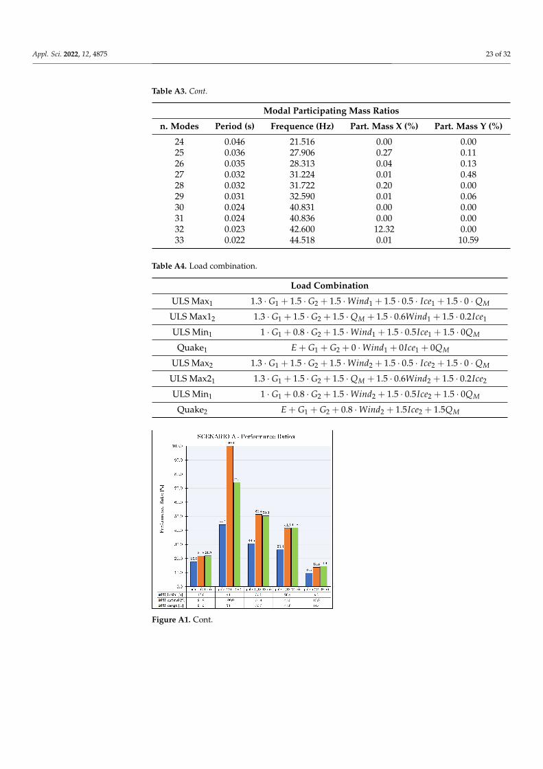
This section details the loads acting on the structures, from the dead to the variableloads. According to the Italian Standard Regulation NTC2018, the load combinations of theactions have been evaluated at the ultimate limit state (ULS) and, for seismic conditions,at the life safety (LS) limit state. In Appendix A, Table A4 illustrates the most criticalcombinations for both static and dynamic configurations. Partial safety factors γ and

Appl. Sci. 2022, 12, 4875 5 of 32

combination coefficients ψ were adopted in order to consider maximization (positive sign)or minimization (negative sign) of effects both for vertical and horizontal actions.

3.1. Dead Loads

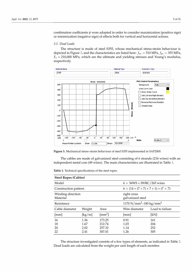
The structure is made of steel S355, whose mechanical stress-strain behaviour isdepicted in Figure 3, and the characteristics are listed here: fus = 510 MPa, fys = 355 MPa,Es = 210,000 MPa, which are the ultimate and yielding stresses and Young’s modulus,respectively.

Figure 3. Mechanical stress–strain behaviour of steel S355 implemented in SAP2000.

The cables are made of galvanized steel consisting of 6 strands (216 wires) with anindependent metal core (49 wires). The main characteristics are illustrated in Table 1.

Table 1. Technical specifications of the steel ropes.

Steel Ropes (Cables)

Model 6 × 36WS + IWRC/265 wires

Construction pattern 6 × (14 + (7 + 7) + 7 + 1) + (7 × 7)

Winding direction right crossMaterial galvanized steel

Resistance 1170 N/mm2–180 kg/mm2

Cable diameter Weight Area Wire diameter Load to failure

[mm] [kg/m] [mm2] [mm] [kN]

16 1.36 173.25 0.91 16118 1.67 212.74 1.03 20420 2.02 257.32 1.14 25222 2.41 307.01 1.26 305

The structure investigated consists of a few types of elements, as indicated in Table 2.Dead loads are calculated from the weight per unit length of each member.

Appl. Sci. 2022, 12, 4875 6 of 32

Table 2. Computation of the dead loads.

Computation of Dead Loads

Profile [mm] w[kg/m]

Length [m] n° Wtot[kg]

CircularD168.3 × 12.5 48 6 5 1440D168.3 × 12.5 48 5.65 2 543

Rectangular60 × 40 × 3 4.35 3.16 9 12460 × 40 × 3 4.35 1.8 9 71100 × 40 × 3 6.13 0.45 6 17

Rope

D16 1.3667 12.45 3 51D16 1.3667 15.44 3 63D16 1.3667 24.43 9 300D16 1.3667 5.76 3 24D16 1.3667 8.46 3 35

2651 Kg

The non-structural dead loads originate from the wiring weight and the steel ladderfor inspection and maintenance. This load results in 0.3 kN/m. Antennas and parabo-las represent the weight of the equipment. Two groups of three antennas are located at26.00 and 29.25 m in height, with a 120° in mutual spacing. The first one is the modelAOC4518R7v06 produced by Huawei®. The second one is the model 6888670N manufac-tured by Amphenol®. Finally, there are three parabolas located at 23.15 m height, spaced120° apart from each other, 30 cm in diameter. Tables 3 and 4 detail the weight of theequipment and the non-structural dead loads.

Table 3. Weight of equipment, H, W, and D stand for height, width, and depth.

Typology Model No Elevation [m] H×W×D [mm] Self-Weight [kg] Clamps [kg] Total [kg]

Antenna AOC4518R7v06 3 29.25 1509 × 469 × 206 39.3 2 × 5.8 153Antenna 6888670N 3 26 1997 × 305 × 163 32 2 × 3.9 119Parabola n.d 3 23.15 Diameter = 300 15 2.2 51.6

Table 4. Non-structural dead loads.

Item qk [kN/m] Qk [kN]

Steel ladder,other

0.3 -

Antenna - 1.53Antenna - 1.19Parabolas - 0.52

3.2. Variable Loads

In this section, the detailed load modeling phase, for each variable load considered, isdescribed. With specific reference to the wind action evaluation, the drag and lift forces arecalculated according to the CNR-DT 207 R1/2018 [43]. The relationship between inertiaand viscous forces, i.e., how wind load impacts to the surface, is taken into account withthe Reynold’s number Re with the following expression:

Re(z) =l · vm(z)

ν(1)

where z is the elevation, l is the characteristic length, vm is the averaged wind speed, whileν is the kinematic viscosity of air (ν = 15× 10−6 m2/s).

Appl. Sci. 2022, 12, 4875 7 of 32

3.2.1. Maintenance and Repairing Loads

Following the Italian national recommendations [44], it is supposed that a typicalsituation of inspection or maintenance is performed by an operator working on the steelladder. A concentrated load of 120 kg is applied at the top of the tower. Despite that, itis reasonable to believe that the operator could work by using a basket elevator, withoutloading the structure.

3.2.2. Wind Loads

The wind action was evaluated according to the Italian recommendations in [43].Firstly, the peak kinetic pressure (qp) was evaluated as follows:

qp =12· ρ · v2

r · ce(z) (2)

where p is the kinetic pressure, while:

• ρ is the air density;• v2

r is the reference wind velocity;• ce is the exposure coefficient, varying with the elevation z of the structure.

For this purpose, the equivalent longitudinal or drag forces, fD, and transverse or liftforce, fL, are evaluated as follows:

fdrag = qp(z) · l · cdrag; fli f t = qp(z) · b · cli f t (3)

where

• qp(z) is the peak kinetic pressure evaluated at height z;• l is the characteristic element size;• b is the reference transverse dimension of the section;• cdrag and cli f t are the longitudinal and transverse dynamic coefficients.

Drag D and Lift L forces are reported in Tables A2 and A3.

3.2.3. Ice Load

Ice and snow attached to the structural surface can significantly increase the variableloads in flexible and light structures. In particular, the radio mast is very sensitive tochanges in the wind-exposed surface. In addition, the ice covering can increase the volumeand the surface of the structural elements more than twice due to the low thickness of thecentral pole. The recommendations in [43] provide several scenarios for ice coverings. Inthe absence of more detailed evaluations, it is customary to consider an ice sleeve formationthat is 12.5 mm thick. After the estimate of the wind loads, the influence of the ice sleeveformation on the structure is considered by assuming an additional exposed surface equalto 15% of the original one.

3.2.4. Seismic Action

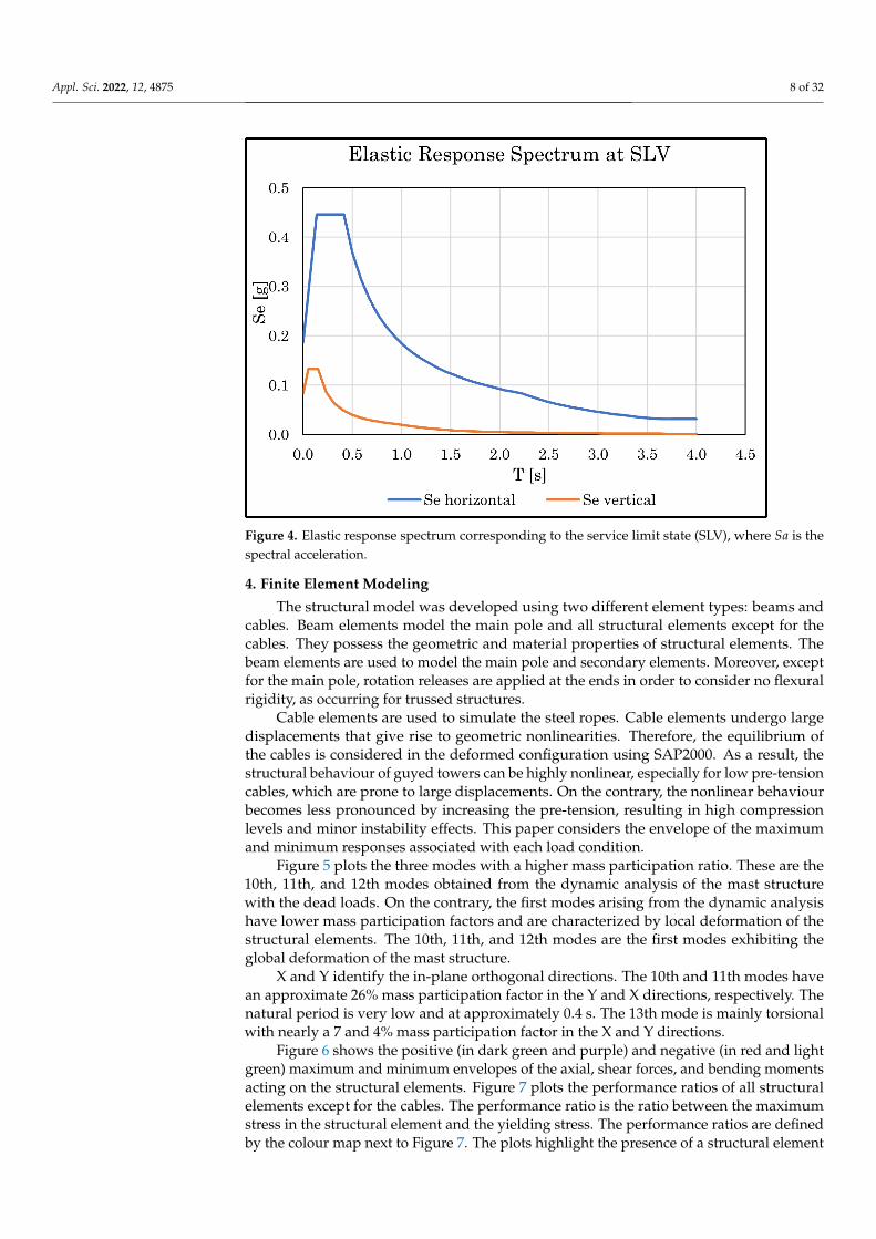
Seismic action is evaluated according to the Italian seismic hazard map [44]. A lineardynamic analysis with seismic elastic response spectrum corresponding to the service limitstate was carried out. Specifically, seismic actions are considered as acting independentlyin the X and Y plane directions.

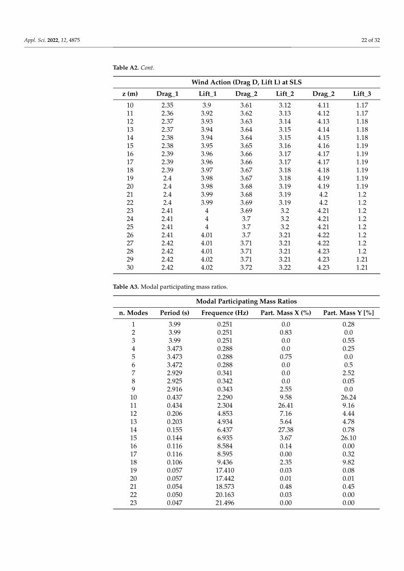
The elastic response spectrum considered in the analysis was calculated by consideringthe topographic category of the site and geometry of the building (Figure 4). The first33 vibration modes of the structure are included in the analysis, to reach 85% of the totalparticipating mass according to the national regulations in [44]. The mass participatingratios are listed in Appendix A.

Appl. Sci. 2022, 12, 4875 8 of 32

Figure 4. Elastic response spectrum corresponding to the service limit state (SLV), where Sa is thespectral acceleration.

4. Finite Element Modeling

The structural model was developed using two different element types: beams andcables. Beam elements model the main pole and all structural elements except for thecables. They possess the geometric and material properties of structural elements. Thebeam elements are used to model the main pole and secondary elements. Moreover, exceptfor the main pole, rotation releases are applied at the ends in order to consider no flexuralrigidity, as occurring for trussed structures.

Cable elements are used to simulate the steel ropes. Cable elements undergo largedisplacements that give rise to geometric nonlinearities. Therefore, the equilibrium ofthe cables is considered in the deformed configuration using SAP2000. As a result, thestructural behaviour of guyed towers can be highly nonlinear, especially for low pre-tensioncables, which are prone to large displacements. On the contrary, the nonlinear behaviourbecomes less pronounced by increasing the pre-tension, resulting in high compressionlevels and minor instability effects. This paper considers the envelope of the maximumand minimum responses associated with each load condition.

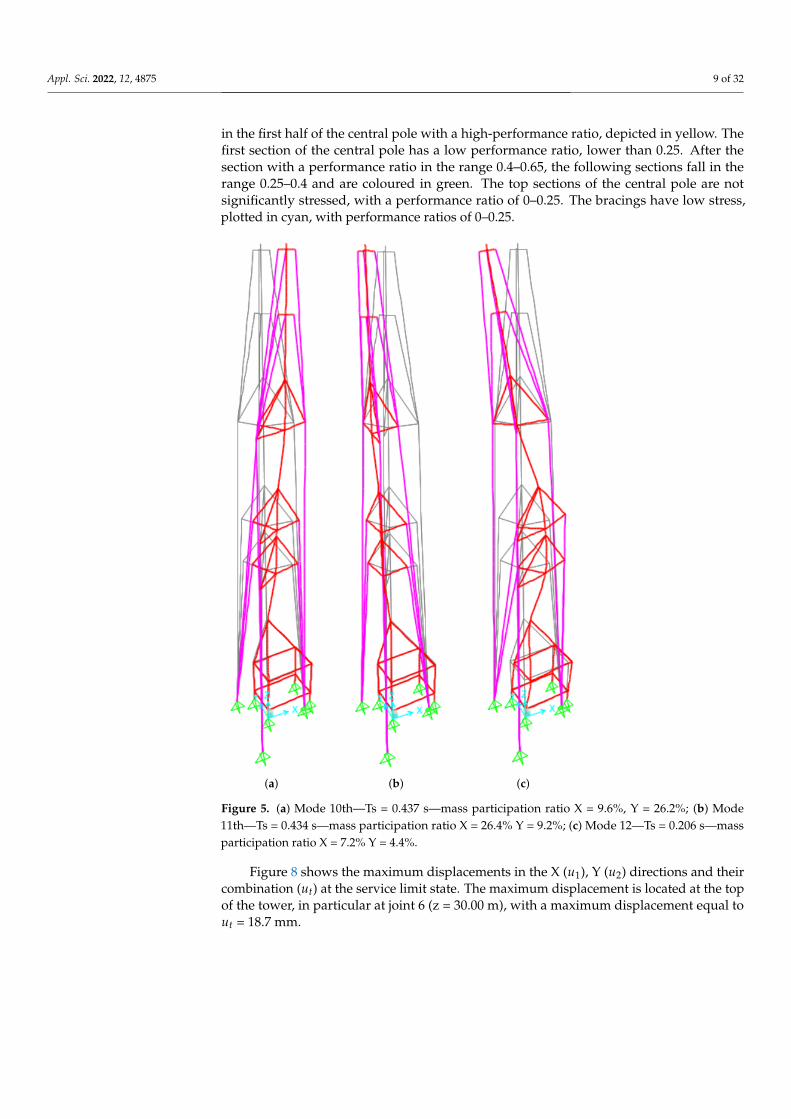
Figure 5 plots the three modes with a higher mass participation ratio. These are the10th, 11th, and 12th modes obtained from the dynamic analysis of the mast structurewith the dead loads. On the contrary, the first modes arising from the dynamic analysishave lower mass participation factors and are characterized by local deformation of thestructural elements. The 10th, 11th, and 12th modes are the first modes exhibiting theglobal deformation of the mast structure.

X and Y identify the in-plane orthogonal directions. The 10th and 11th modes havean approximate 26% mass participation factor in the Y and X directions, respectively. Thenatural period is very low and at approximately 0.4 s. The 13th mode is mainly torsionalwith nearly a 7 and 4% mass participation factor in the X and Y directions.

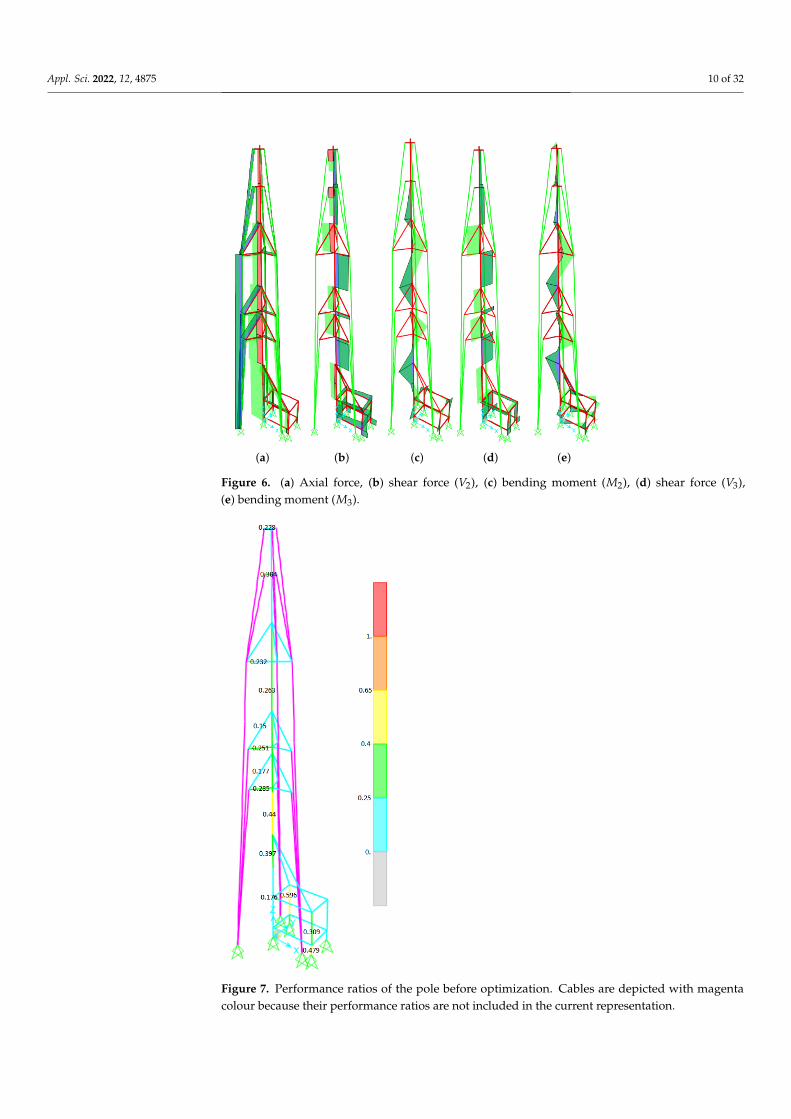
Figure 6 shows the positive (in dark green and purple) and negative (in red and lightgreen) maximum and minimum envelopes of the axial, shear forces, and bending momentsacting on the structural elements. Figure 7 plots the performance ratios of all structuralelements except for the cables. The performance ratio is the ratio between the maximumstress in the structural element and the yielding stress. The performance ratios are definedby the colour map next to Figure 7. The plots highlight the presence of a structural element

Appl. Sci. 2022, 12, 4875 9 of 32

in the first half of the central pole with a high-performance ratio, depicted in yellow. Thefirst section of the central pole has a low performance ratio, lower than 0.25. After thesection with a performance ratio in the range 0.4–0.65, the following sections fall in therange 0.25–0.4 and are coloured in green. The top sections of the central pole are notsignificantly stressed, with a performance ratio of 0–0.25. The bracings have low stress,plotted in cyan, with performance ratios of 0–0.25.

(a) (b) (c)

Figure 5. (a) Mode 10th—Ts = 0.437 s—mass participation ratio X = 9.6%, Y = 26.2%; (b) Mode11th—Ts = 0.434 s—mass participation ratio X = 26.4% Y = 9.2%; (c) Mode 12—Ts = 0.206 s—massparticipation ratio X = 7.2% Y = 4.4%.

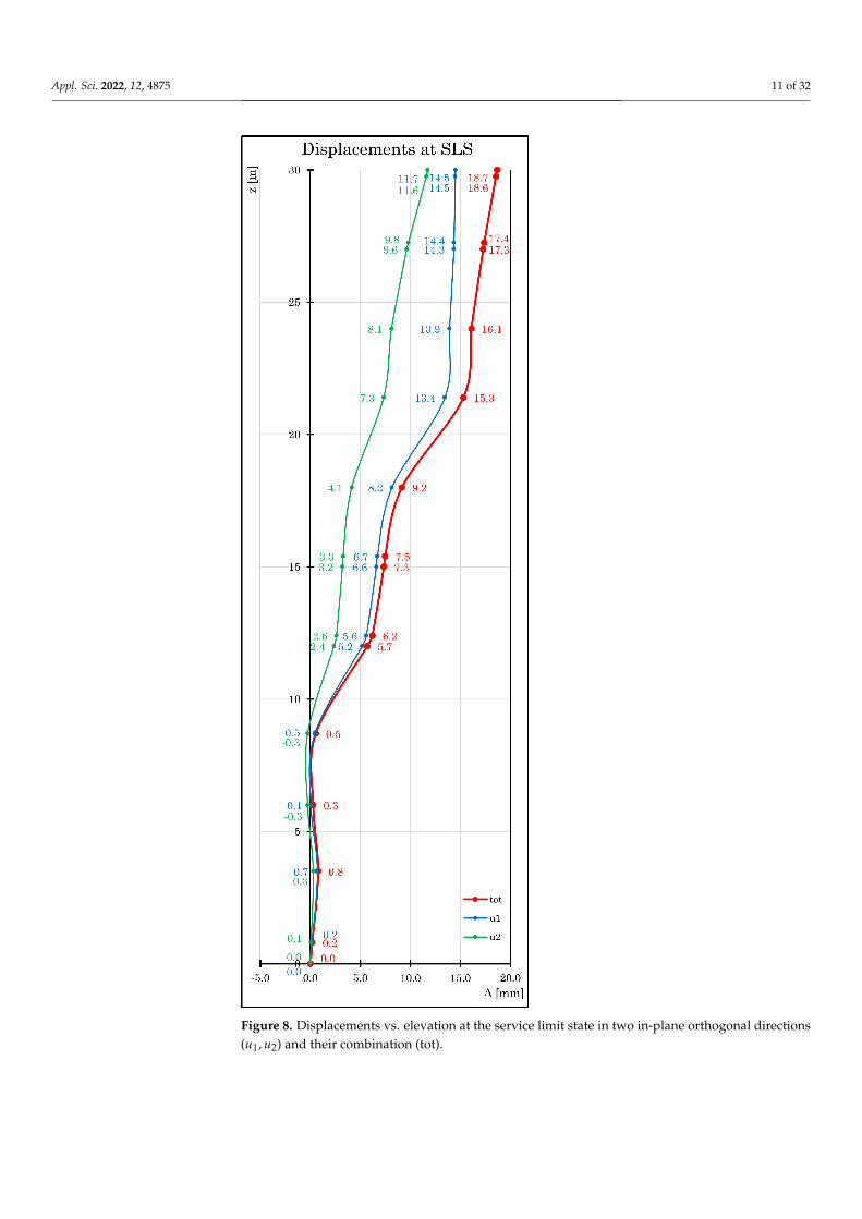
Figure 8 shows the maximum displacements in the X (u1), Y (u2) directions and theircombination (ut) at the service limit state. The maximum displacement is located at the topof the tower, in particular at joint 6 (z = 30.00 m), with a maximum displacement equal tout = 18.7 mm.

Appl. Sci. 2022, 12, 4875 10 of 32

(a) (b) (c) (d) (e)

Figure 6. (a) Axial force, (b) shear force (V2), (c) bending moment (M2), (d) shear force (V3),(e) bending moment (M3).

Figure 7. Performance ratios of the pole before optimization. Cables are depicted with magentacolour because their performance ratios are not included in the current representation.

Appl. Sci. 2022, 12, 4875 11 of 32

Figure 8. Displacements vs. elevation at the service limit state in two in-plane orthogonal directions(u1, u2) and their combination (tot).

Appl. Sci. 2022, 12, 4875 12 of 32

5. Structural Optimization

In optimization problems, the main goal is to find the best conditions in terms of theoptimal set of design parameters collected in the design vector x, which minimizes an ob-jective function (OF) f (x) [45–47]. These problems can be categorized into single-objectiveor multi-objective based on the number of OFs involved, and a further classification isbased on the presence (or not) of constraints [48–50]. In the structural optimization field, itis common to deal with constrained optimization, whose general statement is [51]:

minx∈Ω f (x)

s.t. gq(x) ≤ 0 ∀q = 1, . . . , nq

hr(x) = 0 ∀r = 1, . . . , nr

(4)

where x = x1, . . . , xj, . . . , xnT is the design vector to be optimized, whose terms arelimited into a hyper-rectangular multidimensional box-type search space domain of interestdenoted as Ω, given by the Cartesian product of the range of interest of each j-th of eachdesign variable bounded in [xl

j, xuj ], Ω = [xl

1, xu1 ]× . . .× [xl

j, xuj ]× . . .× [xl

n, xun]. The term

gq(x) in (4) denotes inequality constraints whereas hr(x) are equality ones, which furtherreduce the feasible search space inside Ω. In structural optimization, it is typical to dealwith inequality constraints, and a common goal is to minimize the global cost of thestructure. Since this involves many terms, the main attempt is minimizing the self-weightof the structure, indirectly connected to material cost, i.e., material usage and naturalresources consumption [51]. Several strategies have been developed over the years tohandle constraints [52–54]. In the present work, the penalty function-based approach wasimplemented due to its simplicity, allowing converting the problem with OF f (x) into anew unconstrained version φ(x):

minx∈Ωφ(x)) = min

x∈Ω f (x) + H(x) (5)

where H(x) is the penalty function. Adopting a static-penalty strategy, H(x), assume thisform [55,56]

Hs(x) = w1HNVC(x) + w2HSVC(x) (6)

where HNVC is the number of violated constraints and HSVC is the sum of all violations:

HSVC(x) =np

∑p=1

max0, gp(x) (7)

w1 and w2 are the violation control parameters, whose numerical values are assumed equalto w1 = w2 = 100 following [55].

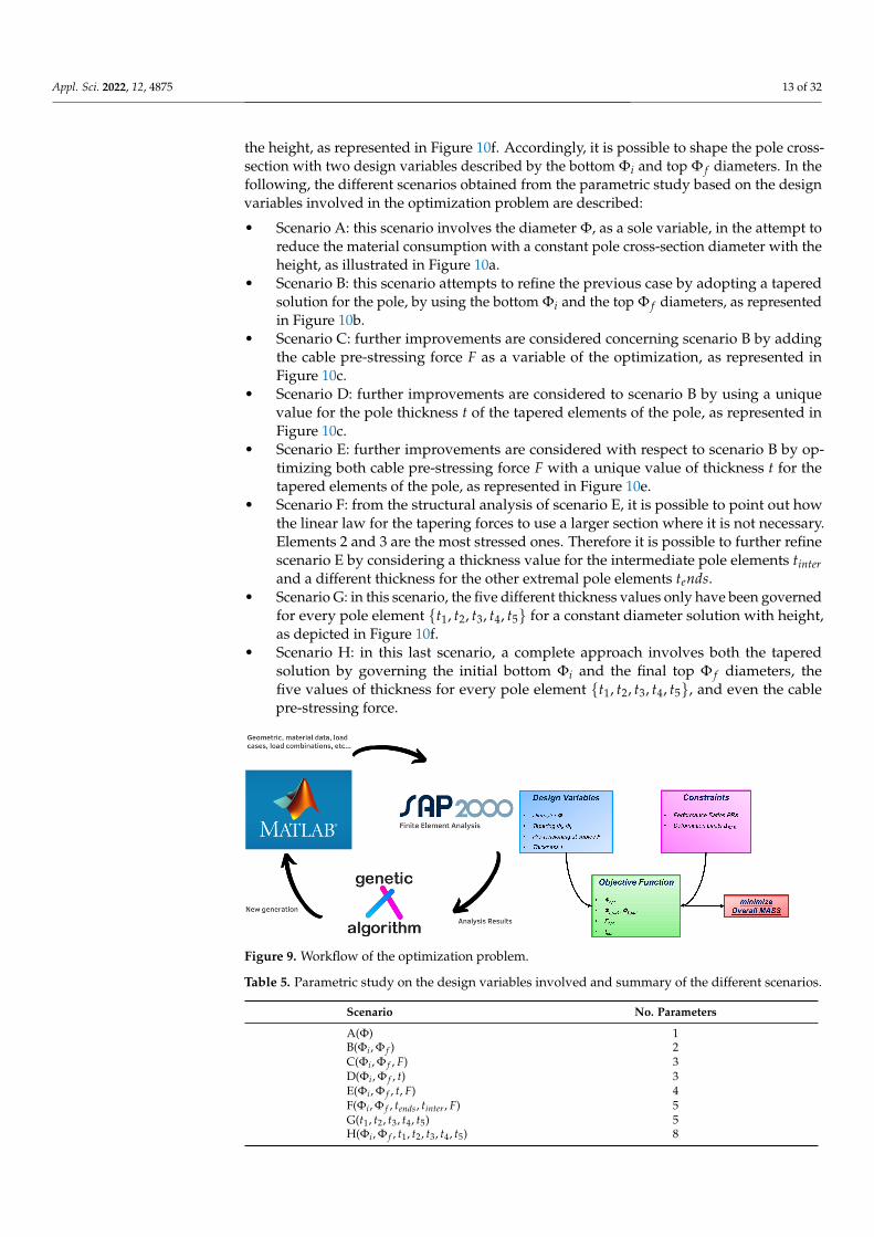
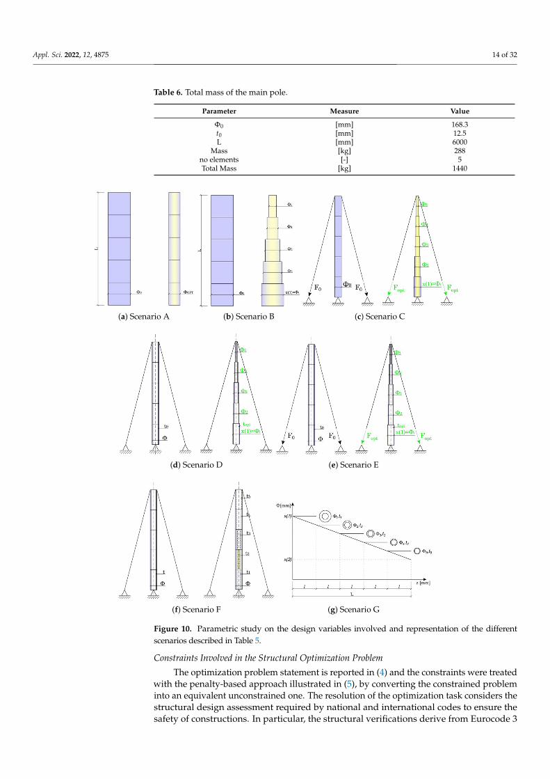
In the current study, the authors carried out a parametric study on the design variablesof the guyed mast. This fact has led to eight different scenarios, summarized in Table 5. Inaddition, the starting initial values of the design parameter are listed in Table 6, while thegeneral optimization workflow is illustrated in Figure 9. To compare the results, the focusis related only to the performance ratios PR of the central pole of the guyed radio mast,being the pole the most stressed element. It consists of five segments 6.00 m long with thesame cross-section. Thus, starting from the ground level:

1. Pole1 (0.00 to 6.00 m);2. Pole2 (6.00 to 12.00 m);3. Pole3 (12.00 to 18.00 m);4. Pole4 (18.00 to 24.00 m);5. Pole5 (24.00 to 30.00 m).

Starting with a constant diameter of the cross-section for the pole, at the end of theoptimization, it is advisable to find a tapered solution following a linear relationship with

Appl. Sci. 2022, 12, 4875 13 of 32

the height, as represented in Figure 10f. Accordingly, it is possible to shape the pole cross-section with two design variables described by the bottom Φi and top Φ f diameters. In thefollowing, the different scenarios obtained from the parametric study based on the designvariables involved in the optimization problem are described:

• Scenario A: this scenario involves the diameter Φ, as a sole variable, in the attempt toreduce the material consumption with a constant pole cross-section diameter with theheight, as illustrated in Figure 10a.

• Scenario B: this scenario attempts to refine the previous case by adopting a taperedsolution for the pole, by using the bottom Φi and the top Φ f diameters, as representedin Figure 10b.

• Scenario C: further improvements are considered concerning scenario B by addingthe cable pre-stressing force F as a variable of the optimization, as represented inFigure 10c.

• Scenario D: further improvements are considered to scenario B by using a uniquevalue for the pole thickness t of the tapered elements of the pole, as represented inFigure 10c.

• Scenario E: further improvements are considered with respect to scenario B by op-timizing both cable pre-stressing force F with a unique value of thickness t for thetapered elements of the pole, as represented in Figure 10e.

• Scenario F: from the structural analysis of scenario E, it is possible to point out howthe linear law for the tapering forces to use a larger section where it is not necessary.Elements 2 and 3 are the most stressed ones. Therefore it is possible to further refinescenario E by considering a thickness value for the intermediate pole elements tinterand a different thickness for the other extremal pole elements tends.

• Scenario G: in this scenario, the five different thickness values only have been governedfor every pole element t1, t2, t3, t4, t5 for a constant diameter solution with height,as depicted in Figure 10f.

• Scenario H: in this last scenario, a complete approach involves both the taperedsolution by governing the initial bottom Φi and the final top Φ f diameters, thefive values of thickness for every pole element t1, t2, t3, t4, t5, and even the cablepre-stressing force.

Figure 9. Workflow of the optimization problem.

Table 5. Parametric study on the design variables involved and summary of the different scenarios.

Scenario No. Parameters

A(Φ) 1B(Φi , Φ f ) 2C(Φi , Φ f , F) 3D(Φi , Φ f , t) 3E(Φi , Φ f , t, F) 4F(Φi , Φ f , tends, tinter , F) 5G(t1, t2, t3, t4, t5) 5H(Φi , Φ f , t1, t2, t3, t4, t5) 8

Appl. Sci. 2022, 12, 4875 14 of 32

Table 6. Total mass of the main pole.

Parameter Measure Value

Φ0 [mm] 168.3t0 [mm] 12.5L [mm] 6000

Mass [kg] 288no elements [-] 5Total Mass [kg] 1440

(a) Scenario A (b) Scenario B (c) Scenario C

(d) Scenario D (e) Scenario E

(f) Scenario F (g) Scenario G

Figure 10. Parametric study on the design variables involved and representation of the differentscenarios described in Table 5.

Constraints Involved in the Structural Optimization Problem

The optimization problem statement is reported in (4) and the constraints were treatedwith the penalty-based approach illustrated in (5), by converting the constrained probleminto an equivalent unconstrained one. The resolution of the optimization task considers thestructural design assessment required by national and international codes to ensure thesafety of constructions. In particular, the structural verifications derive from Eurocode 3

Appl. Sci. 2022, 12, 4875 15 of 32

(EN 1993-1-1: 2005) and are referred to the ultimate limit state (ULS). The design verifica-tions include tensile, compression, and buckling verification, and a combined assessment,such as the interaction capacity according to Annex B of the Eurocode 3:

DC

=NEd

χy A fykγM1

+ kyyMy,Ed

χLTWpl,y fykγM1

+ kyzMz,EdWpl,z fyk

γM1

≤ 1 (8)

DC

=NEd

χz A fykγM1

+ kzyMy,Ed

χLTWpl,y fykγM1

+ kzzMz,EdWpl,z fyk

γM1

≤ 1 (9)

where D stands for the demand and C stands for the capacity of the structure. Specifically,NEd is the acting axial force, whereas My,Ed and Mz,Ed represent the acting bending mo-ments in the two principal directions of a planar local reference system centered on thecross section center of gravity. A is the cross section area of the pole, Wpl,y and Wpl,z arethe plastic section modulus in the two principal directions, fyk is the yielding strength ofthe steel, whereas γM1 is the partial safety factor for instability conditions, equal to 1.05from the Italian National Annex. χLT is the reduction factor for lateral–torsional buckling,whereas kyy, kyz, kzy, and kzz are interaction factors whose values are derived accordingto two alternative approaches based on Annex A (method 1)and Annex B (method 2). Theglobal structural deformation referred to the service limit state (SLS) has also been consid-ered by verifying the top displacement of the mast. Specific recommendations for guyedmast structures are missing in national and international codes. Therefore, the authorsadopted the suggestions defined in the Italian Technical Code NTC2018 (D.M.17/01/2018)reported in Chapter 4.2.4.2.2 Table 4.2.XIII related to limitations of lateral displacementsof steel multi-storey frame structures. These limitations express a threshold condition interms of the total height of the structure H:

δSLS,top ≤ δSLS,top,lim =H

500=

30000 mm500

= 60 mm (10)

Since this condition is specific for steel multi-storey frame structures, the authors willassume this value as a reasonable choice to ensure service life assessment and preservationof working conditions of the telecommunication guyed mast tower. In the next section, adiscussion on the results is carried out.

6. Results and Discussion

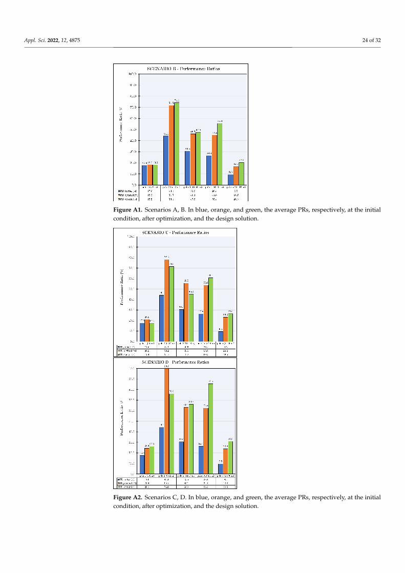
The paper compares the outcomes of the size and shape optimization in eight differentscenarios, distinguished by different design variables. Scenario A is associated with theworst improvement of the structural performance since a single diameter is used for thecentral pole. Additionally, industrial steel profiles do not cover all possible ranges of thediameter. Improvements in the structural performance and weight reduction are achievedin the following scenarios when the search space becomes larger by increasing the numberof design variables.

Scenario B introduces the tapering of the central pole with a linear variation from thebottom to the top. In this case, the optimal solution is affected by intermediate sections,which are more stressed. Consequently, the end cross-sections are over-estimated. Inresponse to that, Scenario F introduces the linear tapering of the tube thickness tends,tinterto enhance the performance of the optimal solution. Parallelly, in Scenario G, five differentthicknesses are adopted (t1, t2, t3, t4, t5), and the results are analogue to case F. Therefore,the thickness of the steel members is a suitable optimization parameter. At the sametime, the diameter alone is not capable of returning attractive solutions because a linearinterpolation trend is used. In addition, lower and upper limits were imposed for d andt. In particular, for this kind of structure, a minimum diameter dmin ≥ 100 mm and aminimum thickness tmin ≥ 3 mm was imposed.

Appl. Sci. 2022, 12, 4875 16 of 32

The cross-section area depends on the square of the thickness. Therefore, smallchanges in t significantly affect the resulting area. Conversely, if the diameter is the solesearch space, despite being tapered linearly with height, even significant modificationsmay not produce notable improvements. Still, the increment of design variables involvedin the structural optimization typically increases the computational efforts. However,the scenario with the highest number of variables was characterized by an average timeiteration close to 18s, using a computer with average performance. The computationaleffort cost of the optimization procedure strongly depends on the machine performance,no convergence issues occur. Table 7 lists the average values of performance ratio obtainedfrom the eight optimization scenarios. All scenarios were collected in terms of numberof parameters involved during the analysis. Table 7 proves that the increment in thenumber of design variables is associated with higher performance ratios. The targetof the optimization achieves the best weight reduction, fully exploiting the structuralmaterial, without exceeding the ultimate and service limit states. Table 7 lists three setsof performance ratios: the initial one before optimization, the optimized, and the oneobtained using commercial steel profiles, called the design performance ratio. The averagedperformance ratio is equal to 28% before optimization. It significantly increases fromscenario A, nearly 45%, to scenario G with 68%.

Table 7. Averaged performance ratios obtained in each optimization scenario.

No Parameters PR Initial PR Optimized PR Design

[%] [%] [%]

1

28.0

45.7 40.52 39.5 43.13 50.5 50.64 54.4 585 65.8 60.28 68 66

Essentially related to PR, mass reduction gives an idea about how much lighter (orheavier) the structure becomes due to the optimization process. It directly provides anestimate of cost savings.

Therefore, the results in Table 8 are consistent with the ones in terms of performanceratios, shown in Table 7.

Table 8. Mass values before/after optimization and after proper approximation (design) usingcommercial steel profiles.

No Parameters Initial Mass [kg] Optimized Mass [kg] Design Mass [kg]

1

1440

1003 11762 1051 11113 803 8184 574 5885 403 4538 385 408

Figure 11 shows the optimization results for the Scenario G, in term of the performanceratio obtained by averaging the performance ratios for each structural element. The resultsfor all scenarios are reported in Appendix A. Scenario G, depicted below, exhibits highervalues of the performance ratios. This fact becomes become more evident for poles 2, 3, and4. In these cases, the performance ratios, associated with the design solutions, achievedvalues equal or greater than the optimized one due to the approximation of the designsection adopted. In the post-processing phase, in fact, the optimized section chosen bythe list of the FE software was manually edited since the structural constraint violationor the maximum performance ratio was not reached during to the optimization process.

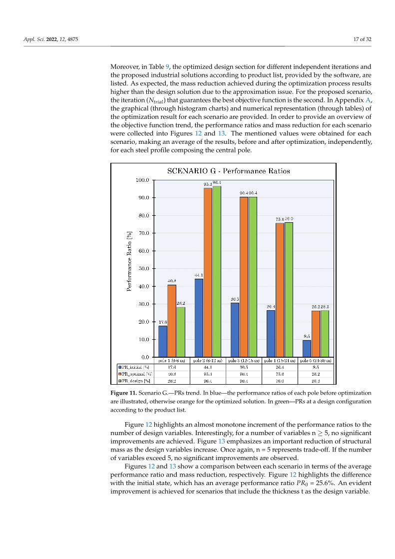
Appl. Sci. 2022, 12, 4875 17 of 32

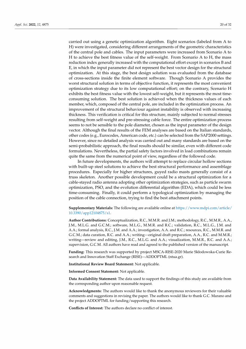
Moreover, in Table 9, the optimized design section for different independent iterations andthe proposed industrial solutions according to product list, provided by the software, arelisted. As expected, the mass reduction achieved during the optimization process resultshigher than the design solution due to the approximation issue. For the proposed scenario,the iteration (Ntrial) that guarantees the best objective function is the second. In Appendix A,the graphical (through histogram charts) and numerical representation (through tables) ofthe optimization result for each scenario are provided. In order to provide an overview ofthe objective function trend, the performance ratios and mass reduction for each scenariowere collected into Figures 12 and 13. The mentioned values were obtained for eachscenario, making an average of the results, before and after optimization, independently,for each steel profile composing the central pole.

Figure 11. Scenario G.—PRs trend. In blue—the performance ratios of each pole before optimizationare illustrated, otherwise orange for the optimized solution. In green—PRs at a design configurationaccording to the product list.

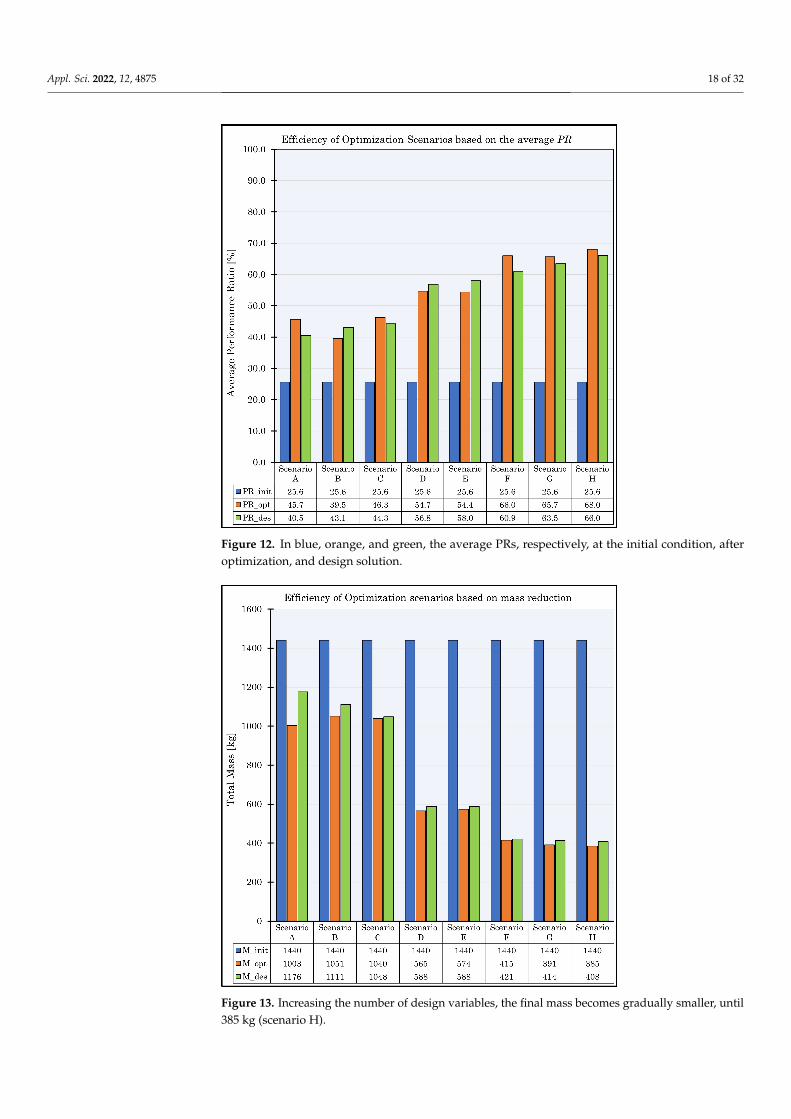
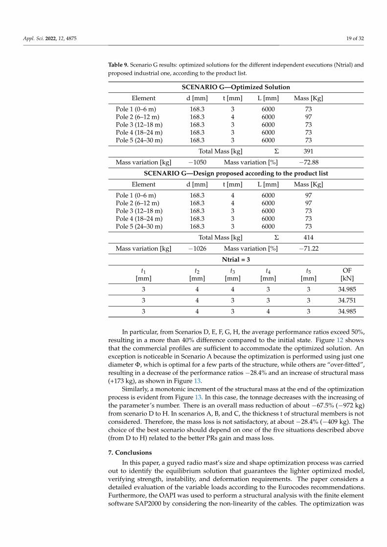
Figure 12 highlights an almost monotone increment of the performance ratios to thenumber of design variables. Interestingly, for a number of variables n ≥ 5, no significantimprovements are achieved. Figure 13 emphasizes an important reduction of structuralmass as the design variables increase. Once again, n = 5 represents trade-off. If the numberof variables exceed 5, no significant improvements are observed.

Figures 12 and 13 show a comparison between each scenario in terms of the averageperformance ratio and mass reduction, respectively. Figure 12 highlights the differencewith the initial state, which has an average performance ratio PR0 = 25.6%. An evidentimprovement is achieved for scenarios that include the thickness t as the design variable.

Appl. Sci. 2022, 12, 4875 18 of 32

Figure 12. In blue, orange, and green, the average PRs, respectively, at the initial condition, afteroptimization, and design solution.

Figure 13. Increasing the number of design variables, the final mass becomes gradually smaller, until385 kg (scenario H).

Appl. Sci. 2022, 12, 4875 19 of 32

Table 9. Scenario G results: optimized solutions for the different independent executions (Ntrial) andproposed industrial one, according to the product list.

SCENARIO G—Optimized Solution

Element d [mm] t [mm] L [mm] Mass [Kg]

Pole 1 (0–6 m) 168.3 3 6000 73Pole 2 (6–12 m) 168.3 4 6000 97Pole 3 (12–18 m) 168.3 3 6000 73Pole 4 (18–24 m) 168.3 3 6000 73Pole 5 (24–30 m) 168.3 3 6000 73

Total Mass [kg] Σ 391

Mass variation [kg] −1050 Mass variation [%] −72.88

SCENARIO G—Design proposed according to the product list

Element d [mm] t [mm] L [mm] Mass [Kg]

Pole 1 (0–6 m) 168.3 4 6000 97Pole 2 (6–12 m) 168.3 4 6000 97Pole 3 (12–18 m) 168.3 3 6000 73Pole 4 (18–24 m) 168.3 3 6000 73Pole 5 (24–30 m) 168.3 3 6000 73

Total Mass [kg] Σ 414

Mass variation [kg] −1026 Mass variation [%] −71.22

Ntrial = 3

t1 t2 t3 t4 t5 OF[mm] [mm] [mm] [mm] [mm] [kN]

3 4 4 3 3 34.985

3 4 3 3 3 34.751

3 4 3 4 3 34.985

In particular, from Scenarios D, E, F, G, H, the average performance ratios exceed 50%,resulting in a more than 40% difference compared to the initial state. Figure 12 showsthat the commercial profiles are sufficient to accommodate the optimized solution. Anexception is noticeable in Scenario A because the optimization is performed using just onediameter Φ, which is optimal for a few parts of the structure, while others are “over-fitted”,resulting in a decrease of the performance ratios −28.4% and an increase of structural mass(+173 kg), as shown in Figure 13.

Similarly, a monotonic increment of the structural mass at the end of the optimizationprocess is evident from Figure 13. In this case, the tonnage decreases with the increasing ofthe parameter’s number. There is an overall mass reduction of about −67.5% (−972 kg)from scenario D to H. In scenarios A, B, and C, the thickness t of structural members is notconsidered. Therefore, the mass loss is not satisfactory, at about −28.4% (−409 kg). Thechoice of the best scenario should depend on one of the five situations described above(from D to H) related to the better PRs gain and mass loss.

7. Conclusions

In this paper, a guyed radio mast’s size and shape optimization process was carriedout to identify the equilibrium solution that guarantees the lighter optimized model,verifying strength, instability, and deformation requirements. The paper considers adetailed evaluation of the variable loads according to the Eurocodes recommendations.Furthermore, the OAPI was used to perform a structural analysis with the finite elementsoftware SAP2000 by considering the non-linearity of the cables. The optimization was

Appl. Sci. 2022, 12, 4875 20 of 32

carried out using a genetic optimization algorithm. Eight scenarios (labeled from A toH) were investigated, considering different arrangements of the geometric characteristicsof the central pole and cables. The input parameters were increased from Scenario A toH to achieve the best fitness value of the self-weight. From Scenario A to H, the massreduction index generally increased with the computational effort except in scenarios B andE, in which the input parameter did not represent the best vector design for the structuraloptimization. At this stage, the best design solution was evaluated from the databaseof cross-sections inside the finite element software. Though Scenario A provides theworst structural solution in terms of objective function, it represents the most convenientoptimization strategy due to its low computational effort; on the contrary, Scenario Hexhibits the best fitness value with the lowest self-weight, but it represents the most time-consuming solution. The best solution is achieved when the thickness values of eachmember, which, composed of the central pole, are included in the optimization process. Animprovement of the structural behaviour against instability is observed with increasingthickness. This verification is critical for this structure, mainly subjected to normal stressesresulting from self-weight and pre-stressing cable force. The entire optimization processseems to not be sensible to the pole diameter, chosen as the input parameter of the designvector. Although the final results of the FEM analyses are based on the Italian standards,other codes (e.g., Eurocodes, American code, etc.) can be selected from the SAP2000 settings.However, since no detailed analysis was carried out and many standards are based on thesemi-probabilistic approach, the final results should be similar, even with different codeformulations. Nevertheless, the partial safety factors involved in load combinations remainquite the same from the numerical point of view, regardless of the followed code.

In future developments, the authors will attempt to replace circular hollow sectionswith built-up steel solutions to achieve the best structural performance and assemblageprocedures. Especially for higher structures, guyed radio masts generally consist of atruss skeleton. Another possible development could be a structural optimization for acable-stayed radio antenna adopting other optimization strategies, such as particle swarmoptimization, PSO, and the evolution differential algorithm (EDA), which could be lesstime-consuming. Finally, it could perform a typological optimization by managing theposition of the cable connection, trying to find the best attachment points.

Supplementary Materials: The following are available online at https://www.mdpi.com/article/10.3390/app12104875/s1.

Author Contributions: Conceptualization, R.C., M.M.R. and J.M.; methodology, R.C., M.M.R., A.A.,J.M., M.L.G. and G.C.M.; software, M.L.G., M.M.R. and R.C.; validation, R.C., M.L.G., J.M. andA.A.; formal analysis, R.C., J.M. and A.A.; investigation, A.A. and R.C.; resources, R.C., M.M.R. andG.C.M.; data curation, R.C. and A.A.; writing—original draft preparation, A.A., R.C. and M.M.R.;writing—review and editing, J.M., R.C., M.L.G. and A.A.; visualization, M.M.R., R.C. and A.A.;supervision, G.C.M. All authors have read and agreed to the published version of the manuscript.

Funding: This research was supported by project MSCA-RISE-2020 Marie Skłodowska-Curie Re-search and Innovation Staff Exchange (RISE)—ADDOPTML (ntua.gr).

Institutional Review Board Statement: Not applicable.

Informed Consent Statement: Not applicable.

Data Availability Statement: The data used to support the findings of this study are available fromthe corresponding author upon reasonable request.

Acknowledgments: The authors would like to thank the anonymous reviewers for their valuablecomments and suggestions in revising the paper. The authors would like to thank G.C. Marano andthe project ADDOPTML for funding/supporting this research.

Conflicts of Interest: The authors declare no conflict of interest.

Appl. Sci. 2022, 12, 4875 21 of 32

Appendix A

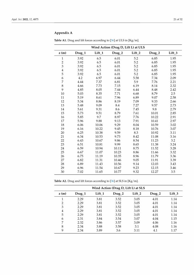
Table A1. Drag and lift forces according to [36] at ULS in [Kg/m].

Wind Action (Drag D, Lift L) at ULS

z (m) Drag_1 Lift_1 Drag_2 Lift_2 Drag_2 Lift_3

1 3.92 6.5 6.01 5.2 6.85 1.952 3.92 6.5 6.01 5.2 6.85 1.953 3.92 6.5 6.01 5.2 6.85 1.954 3.92 6.5 6.01 5.2 6.85 1.955 3.92 6.5 6.01 5.2 6.85 1.956 4.2 6.97 6.44 5.58 7.34 2.097 4.44 7.37 6.81 5.9 7.76 2.218 4.66 7.73 7.15 6.19 8.14 2.329 4.85 8.05 7.44 6.44 8.48 2.42

10 5.03 8.35 7.71 6.68 8.79 2.511 5.19 8.61 7.96 6.89 9.07 2.5812 5.34 8.86 8.19 7.09 9.33 2.6613 5.48 9.09 8.4 7.27 9.57 2.7314 5.61 9.31 8.6 7.45 9.8 2.7915 5.73 9.51 8.79 7.61 10.01 2.8516 5.85 9.7 8.97 7.76 10.22 2.9117 5.96 9.88 9.13 7.91 10.41 2.9718 6.06 10.06 9.29 8.04 10.59 3.0219 6.16 10.22 9.45 8.18 10.76 3.0720 6.25 10.38 9.59 8.3 10.92 3.1121 6.34 10.53 9.73 8.42 11.08 3.1622 6.43 10.67 9.86 8.54 11.23 3.223 6.51 10.81 9.99 8.65 11.38 3.2424 6.59 10.94 10.11 8.75 11.52 3.2825 6.67 11.07 10.23 8.86 11.66 3.3226 6.75 11.19 10.35 8.96 11.79 3.3627 6.82 11.31 10.46 9.05 11.91 3.3928 6.89 11.43 10.56 9.14 12.03 3.4329 6.96 11.54 10.67 9.23 12.15 3.4630 7.02 11.65 10.77 9.32 12.27 3.5

Table A2. Drag and lift forces according to [36] at SLS in [Kg/m].

Wind Action (Drag D, Lift L) at SLS

z (m) Drag_1 Lift_1 Drag_2 Lift_2 Drag_2 Lift_3

1 2.29 3.81 3.52 3.05 4.01 1.142 2.29 3.81 3.52 3.05 4.01 1.143 2.29 3.81 3.52 3.05 4.01 1.144 2.29 3.81 3.52 3.05 4.01 1.145 2.29 3.81 3.52 3.05 4.01 1.146 2.31 3.84 3.54 3.07 4.04 1.157 2.32 3.86 3.57 3.09 4.06 1.168 2.34 3.88 3.58 3.1 4.08 1.169 2.34 3.89 3.6 3.11 4.1 1.17

Appl. Sci. 2022, 12, 4875 22 of 32

Table A2. Cont.

Wind Action (Drag D, Lift L) at SLS

z (m) Drag_1 Lift_1 Drag_2 Lift_2 Drag_2 Lift_3

10 2.35 3.9 3.61 3.12 4.11 1.1711 2.36 3.92 3.62 3.13 4.12 1.1712 2.37 3.93 3.63 3.14 4.13 1.1813 2.37 3.94 3.64 3.15 4.14 1.1814 2.38 3.94 3.64 3.15 4.15 1.1815 2.38 3.95 3.65 3.16 4.16 1.1916 2.39 3.96 3.66 3.17 4.17 1.1917 2.39 3.96 3.66 3.17 4.17 1.1918 2.39 3.97 3.67 3.18 4.18 1.1919 2.4 3.98 3.67 3.18 4.19 1.1920 2.4 3.98 3.68 3.19 4.19 1.1921 2.4 3.99 3.68 3.19 4.2 1.222 2.4 3.99 3.69 3.19 4.2 1.223 2.41 4 3.69 3.2 4.21 1.224 2.41 4 3.7 3.2 4.21 1.225 2.41 4 3.7 3.2 4.21 1.226 2.41 4.01 3.7 3.21 4.22 1.227 2.42 4.01 3.71 3.21 4.22 1.228 2.42 4.01 3.71 3.21 4.23 1.229 2.42 4.02 3.71 3.21 4.23 1.2130 2.42 4.02 3.72 3.22 4.23 1.21

Table A3. Modal participating mass ratios.

Modal Participating Mass Ratios

n. Modes Period (s) Frequence (Hz) Part. Mass X (%) Part. Mass Y [%]

1 3.99 0.251 0.0 0.282 3.99 0.251 0.83 0.03 3.99 0.251 0.0 0.554 3.473 0.288 0.0 0.255 3.473 0.288 0.75 0.06 3.472 0.288 0.0 0.57 2.929 0.341 0.0 2.528 2.925 0.342 0.0 0.059 2.916 0.343 2.55 0.0

10 0.437 2.290 9.58 26.2411 0.434 2.304 26.41 9.1612 0.206 4.853 7.16 4.4413 0.203 4.934 5.64 4.7814 0.155 6.437 27.38 0.7815 0.144 6.935 3.67 26.1016 0.116 8.584 0.14 0.0017 0.116 8.595 0.00 0.3218 0.106 9.436 2.35 9.8219 0.057 17.410 0.03 0.0820 0.057 17.442 0.01 0.0121 0.054 18.573 0.48 0.4522 0.050 20.163 0.03 0.0023 0.047 21.496 0.00 0.00

Appl. Sci. 2022, 12, 4875 23 of 32

Table A3. Cont.

Modal Participating Mass Ratios

n. Modes Period (s) Frequence (Hz) Part. Mass X (%) Part. Mass Y (%)

24 0.046 21.516 0.00 0.0025 0.036 27.906 0.27 0.1126 0.035 28.313 0.04 0.1327 0.032 31.224 0.01 0.4828 0.032 31.722 0.20 0.0029 0.031 32.590 0.01 0.0630 0.024 40.831 0.00 0.0031 0.024 40.836 0.00 0.0032 0.023 42.600 12.32 0.0033 0.022 44.518 0.01 10.59

Table A4. Load combination.

Load Combination

ULS Max1 1.3 · G1 + 1.5 · G2 + 1.5 ·Wind1 + 1.5 · 0.5 · Ice1 + 1.5 · 0 ·QM

ULS Max12 1.3 · G1 + 1.5 · G2 + 1.5 ·QM + 1.5 · 0.6Wind1 + 1.5 · 0.2Ice1

ULS Min1 1 · G1 + 0.8 · G2 + 1.5 ·Wind1 + 1.5 · 0.5Ice1 + 1.5 · 0QM

Quake1 E + G1 + G2 + 0 ·Wind1 + 0Ice1 + 0QM

ULS Max2 1.3 · G1 + 1.5 · G2 + 1.5 ·Wind2 + 1.5 · 0.5 · Ice2 + 1.5 · 0 ·QM

ULS Max21 1.3 · G1 + 1.5 · G2 + 1.5 ·QM + 1.5 · 0.6Wind2 + 1.5 · 0.2Ice2

ULS Min1 1 · G1 + 0.8 · G2 + 1.5 ·Wind2 + 1.5 · 0.5Ice2 + 1.5 · 0QM

Quake2 E + G1 + G2 + 0.8 ·Wind2 + 1.5Ice2 + 1.5QM

Figure A1. Cont.

Appl. Sci. 2022, 12, 4875 24 of 32

Figure A1. Scenarios A, B. In blue, orange, and green, the average PRs, respectively, at the initialcondition, after optimization, and the design solution.

Figure A2. Scenarios C, D. In blue, orange, and green, the average PRs, respectively, at the initialcondition, after optimization, and the design solution.

Appl. Sci. 2022, 12, 4875 25 of 32

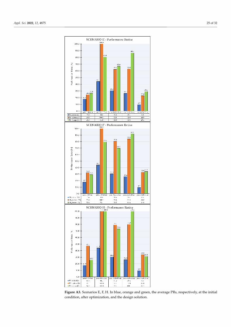
Figure A3. Scenarios E, F, H. In blue, orange and green, the average PRs, respectively, at the initialcondition, after optimization, and the design solution.

Appl. Sci. 2022, 12, 4875 26 of 32

Table A5. Scenario A results: optimized solutions for the different independent executions (Ntrial)and the proposed industrial one, according to the product list.

SCENARIO A—Optimized Solution

Element d [mm] t [mm] L [mm] Mass [Kg]

Pole 1 (0–6 m) 121 12.5 6000 201Pole 2 (6–12 m) 121 12.5 6000 201Pole 3 (12–18 m) 121 12.5 6000 201Pole 4 (18–24 m) 121 12.5 6000 201Pole 5 (24–30 m) 121 12.5 6000 201

Total Mass [kg] Σ 1003

Mass variation [kg] −437 Mass variation [%] −30.36

SCENARIO A—Design proposed according to the product list

Element d [mm] t [mm] L [mm] Mass [Kg]

Pole 1 (0–6 m) 139.7 12.5 6000 235Pole 2 (6–12 m) 139.7 12.5 6000 235Pole 3 (12–18 m) 139.7 12.5 6000 235Pole 4 (18–24 m) 139.7 12.5 6000 235Pole 5 (24–30 m) 139.7 12.5 6000 235

Total Mass [kg] Σ 1176

Mass variation [kg] −264 Mass variation [%] −18.36

Ntrial = 5

Φopt [mm] OF [kN]

121 40.758

121 40.758

121 40.758

121 40.758

122 40.849

Table A6. Scenario B results: optimized solutions for the different independent executions (Ntrial)and the proposed industrial one according to the product list.

SCENARIO B—Optimized Solution

Element d [mm] t [mm] L [mm] Mass [Kg]

Pole 1 (0–6 m) 149 12.5 6000 252Pole 2 (6–12 m) 138 12.5 6000 231Pole 3 (12–18 m) 126 12.5 6000 210Pole 4 (18–24 m) 115 12.5 6000 189Pole 5 (24–30 m) 103 12.5 6000 168

Total Mass [kg] Σ 1051

Mass variation [kg] −389 Mass variation [%] −27.02

SCENARIO B—Design proposed according to product list

Element d [mm] t [mm] L [mm] Mass [Kg]

Pole 1 (0–6 m) 168.3 12.5 6000 288Pole 2 (6–12 m) 139.7 12.5 6000 235Pole 3 (12–18 m) 139.7 12.5 6000 235Pole 4 (18–24 m) 114.3 12.5 6000 188

Appl. Sci. 2022, 12, 4875 27 of 32

Table A6. Cont.

Pole 5 (24–30 m) 101.6 12.5 6000 165

Total Mass [kg] Σ 1111

Mass variation [kg] −329 Mass variation [%] −22.84

Ntrial = 5; best solutions

Φi [mm] Φ f [mm] OF [kN]

148 94 41.248

146 103 41.466

148 94 41.248

146 103 41.466

149 92 41.230

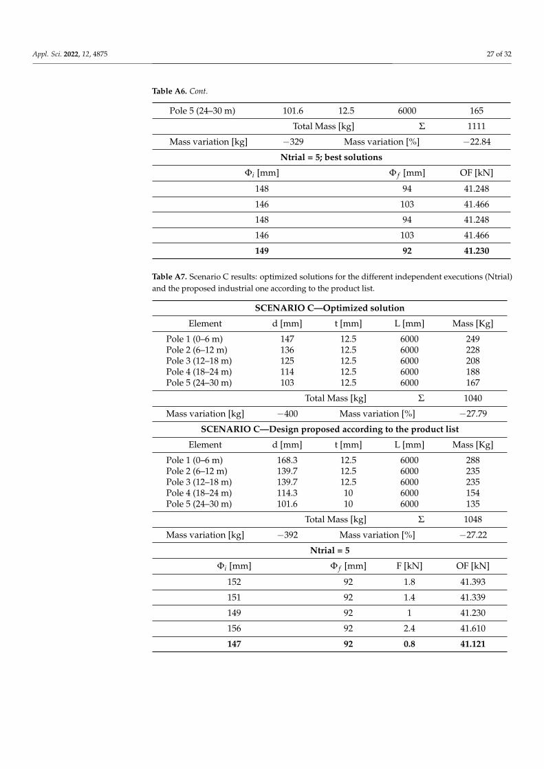
Table A7. Scenario C results: optimized solutions for the different independent executions (Ntrial)and the proposed industrial one according to the product list.

SCENARIO C—Optimized solution

Element d [mm] t [mm] L [mm] Mass [Kg]

Pole 1 (0–6 m) 147 12.5 6000 249Pole 2 (6–12 m) 136 12.5 6000 228Pole 3 (12–18 m) 125 12.5 6000 208Pole 4 (18–24 m) 114 12.5 6000 188Pole 5 (24–30 m) 103 12.5 6000 167

Total Mass [kg] Σ 1040

Mass variation [kg] −400 Mass variation [%] −27.79

SCENARIO C—Design proposed according to the product list

Element d [mm] t [mm] L [mm] Mass [Kg]

Pole 1 (0–6 m) 168.3 12.5 6000 288Pole 2 (6–12 m) 139.7 12.5 6000 235Pole 3 (12–18 m) 139.7 12.5 6000 235Pole 4 (18–24 m) 114.3 10 6000 154Pole 5 (24–30 m) 101.6 10 6000 135

Total Mass [kg] Σ 1048

Mass variation [kg] −392 Mass variation [%] −27.22

Ntrial = 5

Φi [mm] Φ f [mm] F [kN] OF [kN]

152 92 1.8 41.393

151 92 1.4 41.339

149 92 1 41.230

156 92 2.4 41.610

147 92 0.8 41.121

Appl. Sci. 2022, 12, 4875 28 of 32

Table A8. Scenario D results: optimized solutions for the different independent executions (Ntrial)and the proposed industrial one according to the product list.

SCENARIO D—Optimized solution

Element d [mm] t [mm] L [mm] Mass [Kg]

Pole 1 (0–6 m) 161 6 6000 138Pole 2 (6–12 m) 147 6 6000 125Pole 3 (12–18 m) 133 6 6000 113Pole 4 (18–24 m) 120 6 6000 101Pole 5 (24–30 m) 106 6 6000 89

Total Mass [kg] Σ 565

Mass variation [kg] −875 Mass variation [%] −60.75

SCENARIO D—Design proposed according to the product list

Element d [mm] t [mm] L [mm] Mass [Kg]

Pole 1 (0–6 m) 168.3 6 6000 144Pole 2 (6–12 m) 168.3 6 6000 144Pole 3 (12–18 m) 139.7 6 6000 119Pole 4 (18–24 m) 114.3 6 6000 96Pole 5 (24–30 m) 101.6 6 6000 85

Total Mass [kg] Σ 588

Mass variation [kg] −853 Mass variation [%] −59.20

Ntrial = 5

Φi [mm] Φ f [mm] t [mm] OF [kN]

161 92 6 36.465

146 117 7 37.389

162 92 6 36.491

162 92 6 36.491

163 92 6 36.517

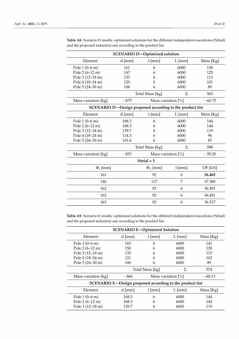
Table A9. Scenario E results: optimized solutions for the different independent executions (Ntrial)and the proposed industrial one according to the product list.

SCENARIO E—Optimized Solution

Element d [mm] t [mm] L [mm] Mass [Kg]

Pole 1 (0–6 m) 165 6 6000 141Pole 2 (6–12 m) 150 6 6000 128Pole 3 (12–18 m) 135 6 6000 115Pole 4 (18–24 m) 121 6 6000 102Pole 5 (24–30 m) 106 6 6000 89

Total Mass [kg] Σ 574

Mass variation [kg] −866 Mass variation [%] −60.13

SCENARIO E—Design proposed according to the product list

Element d [mm] t [mm] L [mm] Mass [Kg]

Pole 1 (0–6 m) 168.3 6 6000 144Pole 2 (6–12 m) 168.3 6 6000 144Pole 3 (12–18 m) 139.7 6 6000 119

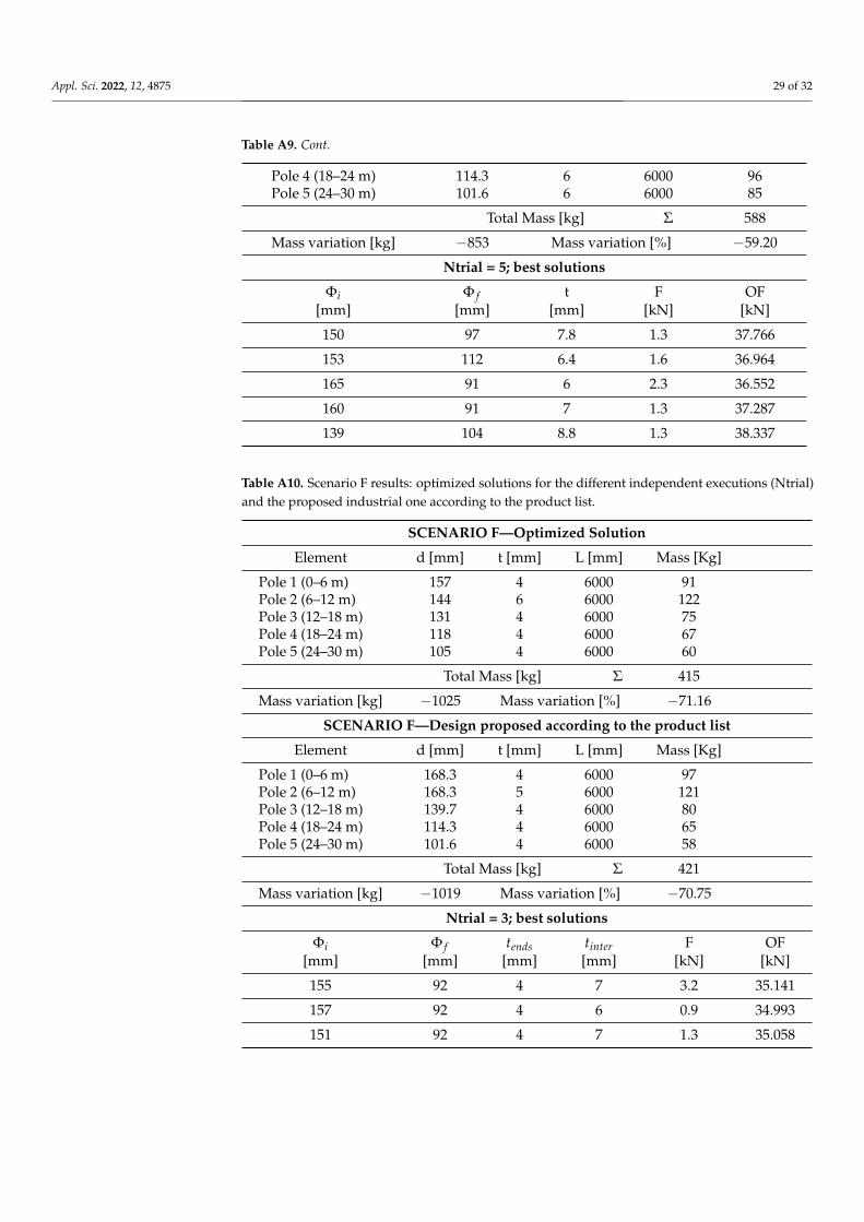
Appl. Sci. 2022, 12, 4875 29 of 32

Table A9. Cont.

Pole 4 (18–24 m) 114.3 6 6000 96Pole 5 (24–30 m) 101.6 6 6000 85

Total Mass [kg] Σ 588

Mass variation [kg] −853 Mass variation [%] −59.20

Ntrial = 5; best solutions

Φi Φ f t F OF[mm] [mm] [mm] [kN] [kN]

150 97 7.8 1.3 37.766

153 112 6.4 1.6 36.964

165 91 6 2.3 36.552

160 91 7 1.3 37.287

139 104 8.8 1.3 38.337

Table A10. Scenario F results: optimized solutions for the different independent executions (Ntrial)and the proposed industrial one according to the product list.

SCENARIO F—Optimized Solution

Element d [mm] t [mm] L [mm] Mass [Kg]

Pole 1 (0–6 m) 157 4 6000 91Pole 2 (6–12 m) 144 6 6000 122Pole 3 (12–18 m) 131 4 6000 75Pole 4 (18–24 m) 118 4 6000 67Pole 5 (24–30 m) 105 4 6000 60

Total Mass [kg] Σ 415

Mass variation [kg] −1025 Mass variation [%] −71.16

SCENARIO F—Design proposed according to the product list

Element d [mm] t [mm] L [mm] Mass [Kg]

Pole 1 (0–6 m) 168.3 4 6000 97Pole 2 (6–12 m) 168.3 5 6000 121Pole 3 (12–18 m) 139.7 4 6000 80Pole 4 (18–24 m) 114.3 4 6000 65Pole 5 (24–30 m) 101.6 4 6000 58

Total Mass [kg] Σ 421

Mass variation [kg] −1019 Mass variation [%] −70.75

Ntrial = 3; best solutions

Φi Φ f tends tinter F OF[mm] [mm] [mm] [mm] [kN] [kN]

155 92 4 7 3.2 35.141

157 92 4 6 0.9 34.993

151 92 4 7 1.3 35.058

Appl. Sci. 2022, 12, 4875 30 of 32

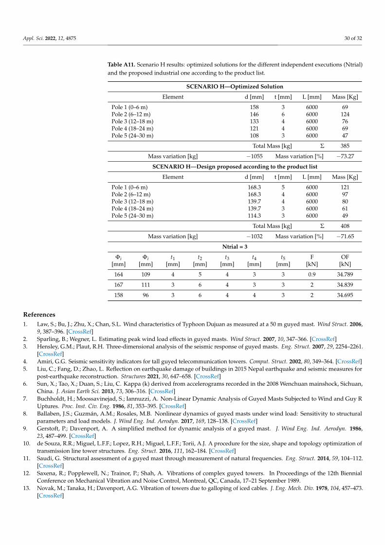
Table A11. Scenario H results: optimized solutions for the different independent executions (Ntrial)and the proposed industrial one according to the product list.

SCENARIO H—Optimized Solution

Element d [mm] t [mm] L [mm] Mass [Kg]

Pole 1 (0–6 m) 158 3 6000 69Pole 2 (6–12 m) 146 6 6000 124Pole 3 (12–18 m) 133 4 6000 76Pole 4 (18–24 m) 121 4 6000 69Pole 5 (24–30 m) 108 3 6000 47

Total Mass [kg] Σ 385

Mass variation [kg] −1055 Mass variation [%] −73.27

SCENARIO H—Design proposed according to the product list

Element d [mm] t [mm] L [mm] Mass [Kg]

Pole 1 (0–6 m) 168.3 5 6000 121Pole 2 (6–12 m) 168.3 4 6000 97Pole 3 (12–18 m) 139.7 4 6000 80Pole 4 (18–24 m) 139.7 3 6000 61Pole 5 (24–30 m) 114.3 3 6000 49

Total Mass [kg] Σ 408

Mass variation [kg] −1032 Mass variation [%] −71.65

Ntrial = 3

Φi Φi t1 t2 t3 t4 t5 F OF[mm] [mm] [mm] [mm] [mm] [mm] [mm] [kN] [kN]

164 109 4 5 4 3 3 0.9 34.789

167 111 3 6 4 3 3 2 34.839

158 96 3 6 4 4 3 2 34.695

References1. Law, S.; Bu, J.; Zhu, X.; Chan, S.L. Wind characteristics of Typhoon Dujuan as measured at a 50 m guyed mast. Wind Struct. 2006,

9, 387–396. [CrossRef]2. Sparling, B.; Wegner, L. Estimating peak wind load effects in guyed masts. Wind Struct. 2007, 10, 347–366. [CrossRef]3. Hensley, G.M.; Plaut, R.H. Three-dimensional analysis of the seismic response of guyed masts. Eng. Struct. 2007, 29, 2254–2261.

[CrossRef]4. Amiri, G.G. Seismic sensitivity indicators for tall guyed telecommunication towers. Comput. Struct. 2002, 80, 349–364. [CrossRef]5. Liu, C.; Fang, D.; Zhao, L. Reflection on earthquake damage of buildings in 2015 Nepal earthquake and seismic measures for

post-earthquake reconstruction. Structures 2021, 30, 647–658. [CrossRef]6. Sun, X.; Tao, X.; Duan, S.; Liu, C. Kappa (k) derived from accelerograms recorded in the 2008 Wenchuan mainshock, Sichuan,

China. J. Asian Earth Sci. 2013, 73, 306–316. [CrossRef]7. Buchholdt, H.; Moossavinejad, S.; Iannuzzi, A. Non-Linear Dynamic Analysis of Guyed Masts Subjected to Wind and Guy R

Uptures. Proc. Inst. Civ. Eng. 1986, 81, 353–395. [CrossRef]8. Ballaben, J.S.; Guzmán, A.M.; Rosales, M.B. Nonlinear dynamics of guyed masts under wind load: Sensitivity to structural

parameters and load models. J. Wind Eng. Ind. Aerodyn. 2017, 169, 128–138. [CrossRef]9. Gerstoft, P.; Davenport, A. A simplified method for dynamic analysis of a guyed mast. J. Wind Eng. Ind. Aerodyn. 1986,

23, 487–499. [CrossRef]10. de Souza, R.R.; Miguel, L.F.F.; Lopez, R.H.; Miguel, L.F.F.; Torii, A.J. A procedure for the size, shape and topology optimization of

transmission line tower structures. Eng. Struct. 2016, 111, 162–184. [CrossRef]11. Saudi, G. Structural assessment of a guyed mast through measurement of natural frequencies. Eng. Struct. 2014, 59, 104–112.

[CrossRef]12. Saxena, R.; Popplewell, N.; Trainor, P.; Shah, A. Vibrations of complex guyed towers. In Proceedings of the 12th Biennial

Conference on Mechanical Vibration and Noise Control, Montreal, QC, Canada, 17–21 September 1989.13. Novak, M.; Tanaka, H.; Davenport, A.G. Vibration of towers due to galloping of iced cables. J. Eng. Mech. Div. 1978, 104, 457–473.

[CrossRef]

Appl. Sci. 2022, 12, 4875 31 of 32

14. Wahba, Y.M.; Madugula, M.K.; Monforton, G.R. Shake Table for Dynamic Testing of Guyed Towers. In Building to Last; ASCE:Reston, VA, USA, 1997; pp. 353–357.

15. Madugula, M.K.; Wahba, Y.M.; Monforton, G.R. Dynamic response of guyed masts. Eng. Struct. 1998, 20, 1097–1101. [CrossRef]16. Luzardo, A.C.; Parnás, V.E.; Rodríguez, P.M. Guy tension influence on the structural behavior of a guyed mast. J. Int. Assoc. Shell

Spat. Struct. 2012, 53, 111–116.17. Davenport, A.; Sparling, B. Dynamic gust response factors for guyed towers. J. Wind Eng. Ind. Aerodyn. 1992, 43, 2237–2248.

[CrossRef]18. Harikrishna, P.; Annadurai, A.; Gomathinayagam, S.; Lakshmanan, N. Full scale measurements of the structural response of a

50 m guyed mast under wind loading. Eng. Struct. 2003, 25, 859–867. [CrossRef]19. Gioffrè, M.; Gusella, V.; Materazzi, A.; Venanzi, I. Removable guyed mast for mobile phone networks: Wind load modeling and

structural response. J. Wind Eng. Ind. Aerodyn. 2004, 92, 463–475. [CrossRef]20. Clobes, M.; Peil, U. Unsteady buffeting wind loads in the time domain and their effect on the life-cycle prediction of guyed masts.

Struct. Infrastruct. Eng. 2011, 7, 187–196. [CrossRef]21. Pezo, M.L.; Bakic, V.V. Numerical determination of drag coefficient for guyed mast exposed to wind action. Eng. Struct. 2014,

62, 98–104. [CrossRef]22. Sparling, B.F. The Dynamic Behavior of Guys and Guyed Masts in Turbulent Winds. Ph.D. Thesis, Western University, London,

ON, Canada, 1995.23. Wahba, Y.; Madugula, M.; Monforton, G. Evaluation of non-linear analysis of guyed antenna towers. Comput. Struct. 1998,

68, 207–212. [CrossRef]24. Madugula, M.K. Dynamic Response of Lattice Towers and Guyed Masts; ASCE Publications: Reston, VA, USA, 2001.25. Orlando, D.; Gonçalves, P.B.; Rega, G.; Lenci, S. Nonlinear dynamics and instability as important design concerns for a guyed

mast. In IUTAM Symposium on Nonlinear Dynamics for Advanced Technologies and Engineering Design; Springer: Berlin/Heidelberg,Germany, 2013; pp. 223–234.

26. Ballaben, J.S.; Rosales, M.B. Nonlinear dynamic analysis of a 3D guyed mast. Nonlinear Dyn. 2018, 93, 1395–1405. [CrossRef]27. Belevicius, R.; Jatulis, D.; Šešok, D. Optimization of tall guyed masts using genetic algorithms. Eng. Struct. 2013, 56, 239–245.

[CrossRef]28. Gawronski, W.; Bienkiewicz, B.; Hill, R. Wind-induced dynamics of a deep space network antenna. J. Sound Vib. 1994, 178, 67–77.

[CrossRef]29. Fujino, Y.; Warnitchai, P.; Pacheco, B. Active Stiffness Control of Cable Vibration. J. Appl. Mech. 1993, 60, 948–953. [CrossRef]30. Lacarbonara, W.; Ballerini, S. Vibration mitigation of guyed masts via tuned pendulum dampers. Struct. Eng. Mech. Int. J. 2009,

32, 517–529. [CrossRef]31. Błachowski, B. Model based predictive control of guyed mast vibration. J. Theor. Appl. Mech. 2007, 45, 405–423.32. Bell, L.C.; Brown, D.M. Guyed tower optimization. Comput. Struct. 1976, 6, 447–450. [CrossRef]33. Thornton, C.H.; Joseph, L.; Scarangello, T. Optimization of tall structures for wind loading. J. Wind Eng. Ind. Aerodyn. 1990,

36, 235–244. [CrossRef]34. Uys, P.; Farkas, J.; Jarmai, K.; Van Tonder, F. Optimisation of a steel tower for a wind turbine structure. Eng. Struct. 2007,

29, 1337–1342. [CrossRef]35. Venanzi, I.; Materazzi, A. Multi-objective optimization of wind-excited structures. Eng. Struct. 2007, 29, 983–990. [CrossRef]36. Zhang, Z.Q.; Li, H.N. Two-level optimization method of transmission tower structure based on ant colony algorithm. In Advanced

Materials Research; Trans Tech Publications Ltd.: Freienbach, Switzerland, 2011; Volume 243, pp. 5849–5853.37. Cucuzza, R.; Costi, C.; Rosso, M.M.; Domaneschi, M.; Marano, G.C.; Masera, D. Optimal strengthening by steel truss arches in

prestressed girder bridges. In Proceedings of the Institution of Civil Engineers—Bridge Engineering; Thomas Telford Ltd.: London,UK, 2021; pp. 1–21. [CrossRef]

38. Luh, G.C.; Lin, C.Y. Optimal design of truss-structures using particle swarm optimization. Comput. Struct. 2011, 89, 2221–2232.[CrossRef]

39. Manuello Bertetto, A.; Marano, G. Numerical and dimensionless analytical solutions for circular arch optimization. Eng. Struct.2022, 253, 113360. [CrossRef]

40. Kaveh, A.; Talatahari, S. Particle swarm optimizer, ant colony strategy and harmony search scheme hybridized for optimizationof truss structures. Comput. Struct. 2009, 87, 267–283. [CrossRef]

41. Deng, Z.Q.; Zhang, Y.; Huang, H.L.; Li, B. Parametric optimization for a tapered deployable mast in an integrated design environ-ment. In Advanced Materials Research; Trans Tech Publications Ltd.: Freienbach, Switzerland, 2012; Volume 346, pp. 426–432.

42. Guo, H.; Li, Z. Structural topology optimization of high-voltage transmission tower with discrete variables. Struct. Multidiscip.Optim. 2011, 43, 851–861. [CrossRef]

43. delle Ricerche, C.N. Istruzioni per la valutazione delle azioni e degli effetti del vento sulle costruzioni. CNR-DT 2009, 207, 2008.44. Mordà, N.; Mancini, A. Norme Tecniche per le Costruzioni (NTC 2018) D. Min. Infrastrutture e Trasporti 17 Gennaio 2018; Ministero

delle Infrastrutture e dei Trasporti: Roma, Italy, 2018.45. Melchiorre, J.; Bertetto, A.M.; Marano, G.C. Application of a Machine Learning Algorithm for the Structural Optimization of

Circular Arches with Different Cross-Sections. J. Appl. Math. Phys. 2021, 9, 1159–1170. [CrossRef]

Appl. Sci. 2022, 12, 4875 32 of 32

46. Rosso, M.M.; Cucuzza, R.; Aloisio, A.; Marano, G.C. Enhanced Multi-Strategy Particle Swarm Optimization for ConstrainedProblems with an Evolutionary-Strategies-Based Unfeasible Local Search Operator. Appl. Sci. 2022, 12, 2285. [CrossRef]

47. Rosso, M.M.; Cucuzza, R.; Di Trapani, F.; Marano, G.C. Nonpenalty machine learning constraint handling using PSO-svm forstructural optimization. Adv. Civ. Eng. 2021, 2021, 6617750. [CrossRef]

48. Rao, S.S. Engineering Optimization: Theory and Practice; John Wiley & Sons: Hoboken, NJ, USA, 2019.49. Aloisio, A.; Pasca, D.P.; Battista, L.; Rosso, M.M.; Cucuzza, R.; Marano, G.; Alaggio, R. Indirect assessment of concrete resistance

from FE model updating and Young’s modulus estimation of a multi-span PSC viaduct: Experimental tests and validation.Elsevier Struct. 2022, 37, 686–697. [CrossRef]

50. Sardone, L.; Rosso, M.M.; Cucuzza, R.; Greco, R.; Marano, G.C. Computational Design of Comparative models and geometricallyconstrained optimization of a multi-domain variable section beam based on Timoshenko model. In Proceedings of theEUROGEN2021, 14TH ECCOMAS Thematic Conference on Evolutionary and Deterministic Methods for Design, Optimizationand Control, Athens, Greece, 28–30 June 2021. [CrossRef]

51. Christensen, P.W.; Klarbring, A. An Introduction to Structural Optimization; Springer Science & Business Media: Berlin/Heidelberg,Germany, 2008; Volume 153.

52. Coello Coello, C.A. Theoretical and numerical constraint-handling techniques used with evolutionary algorithms: A survey ofthe state of the art. Comput. Methods Appl. Mech. Eng. 2002, 191, 1245–1287. [CrossRef]

53. Koziel, S.; Michalewicz, Z. Evolutionary Algorithms, Homomorphous Mappings, and Constrained Parameter Optimization.Evol. Comput. 1999, 7, 19–44. [CrossRef] [PubMed]

54. Michalewicz, Z.; Fogel, D. How to Solve It: Modern Heuristics; Springer Science & Business Media: Berlin/Heidelberg, Ger-many, 2008.

55. Parsopoulos, K.; Vrahatis, M. Unified Particle Swarm Optimization for Solving Constrained Engineering Optimization Problems.In International Conference on Natural Computation; Springer: Berlin/Heidelberg, Germany, 2005; Volume 3612, pp. 582–591.[CrossRef]

56. Coello, C. Self-adaptive penalties for GA-based optimization. In Proceedings of the 1999 Congress on Evolutionary Computation-CEC99 (Cat. No. 99TH8406), Washington, DC, USA, 6–9 July 1999; IEEE: Hoboken, NJ, USA, 1999; Volume 1, pp. 573–580.[CrossRef]