Simulations of ecosystem response during the sapropel S1 deposition event

www.elsevier.com/locate/palaeo

Palaeogeography, Palaeoclimatology, P

Simulations of ecosystem response during the sapropel

S1 deposition event

D. Bianchi a,*, M. Zavatarelli a, N. Pinardi a, R. Capozzi a, L. Capotondi b,

C. Corselli c, S. Masina d

a Universita di Bologna, Centro Interdipartimentale per la Ricerca sulle Scienze Ambientali, Via S. Alberto 163, 48100 Ravenna, Italyb ISMAR, Istituto di Scienze del Mare, C.N.R., Via Gobetti 101, 40129 Bologna, Italy

c Universita di Milano-Bicocca Dipartimento di Scienze Geologiche e Geotecnologiche, Piazza dell’Ateneo Nuovo 1, 20126 Milan, Italyd Istituto Nazionale di Geofisica e Vulcanologia, Via Donato Creti 12, 40128 Bologna, Italy

Accepted 12 September 2005

Abstract

A one-dimensional ecosystem numerical model is used to simulate the ecosystem changes that could have occurred in the open

ocean areas of the Eastern Mediterranean Sea during the Climatic Optimum interval (9500–6000 B.P., Mercone et al. [Mercone, D.,

Thomson, J., Croudace, I.W., Siani, G., Paterne, M., Troelstra, S., 2000. Duration of S1, the most recent sapropel in the eastern

Mediterranean Sea, as indicated by accelerator mass spectrometry radiocarbon and geochemical evidence. Paleoceanography 15,

336–347]). In this period the S1 sapropel was deposited. S1 is the most recent sapropel in the succession of organic carbon-rich

layers intercalated in normal Neogene sedimentary sequences. Different theories have been invoked in order to explain the

deposition of this peculiar layer. Our simulations seem to indicate that the modified thermohaline circulation, supplying oxygen

only in the first 500 m of the water column, is responsible for the sapropel deposition when higher productivity is allowed in the

euphotic zone. The model shows the importance in this process of bacteria that consume oxygen by decomposing the Particulate

Organic Matter (POM) produced in the upper water column. The sinking velocity of POM partially regulates the timescale of the

occurrence of anoxia at the bottom and in the whole water column, allowing the relatively rapid onset of sapropel deposition.

D 2005 Elsevier B.V. All rights reserved.

Keywords: Sapropel; Holocene; Marine ecology; Mediterranean Sea; Ecological modelling

1. Introduction

1.1. Background

The eastern Mediterranean is a concentration basin

with a thermohaline circulation of anti-estuarine type,

maintained by the excess of evaporative losses over the

precipitation and river runoff inputs (Fig. 1). The fresh-

0031-0182/$ - see front matter D 2005 Elsevier B.V. All rights reserved.

doi:10.1016/j.palaeo.2005.09.032

* Corresponding author. Fax: +39 0544937323.

E-mail address: [email protected] (D. Bianchi).

water deficit is compensated by the surface inflow

through the Sicily Channel of the so-called Modified

Atlantic Water (MAW), constituting the surface branch

of the anti-estuarine thermohaline circulation cell. The

returning branch is located at intermediate depths and is

formed by a well-defined water mass, the Levantine

Intermediate Water (LIW), formed in limited areas of

the eastern Mediterranean in winter. The LIW flow

crosses the Sicily Channel and spreads into the western

Mediterranean at a depth range of 300–500 m, exiting

the Mediterranean Sea through the Gibraltar Straits.

alaeoecology 235 (2006) 265–287

Fig. 1. Schematic of the Mediterranean Sea thermohaline circulation. The grey lines indicate the surface/intermediate water mass circulation forced

by Gibraltar Atlantic inflow and Levantine Intermediate Water (LIW) formation processes occurring in the northern Levantine basin. The black lines

indicate the meridional vertical circulation in western and eastern Mediterranean forced by the deep water formation processes occurring in the Gulf

of Lions and in the Southern Adriatic. Redrawn from Pinardi et al. (2005), reprinted with permission.

D. Bianchi et al. / Palaeogeography, Palaeoclimatology, Palaeoecology 235 (2006) 265–287266

The source of the Eastern Mediterranean Deep Water

(EMDW) is located in the Adriatic Sea, but a dramatic

change in the site of the EMDW formation was recently

observed by Roether et al. (1996). The spreading of the

EMDW from its formation area provides the basic

ventilation mechanism for the deep eastern Mediterra-

nean basin.

The anti-estuarine circulation and low river runoff

promote strong oligotrophic conditions in open waters,

revealed by mean primary production rates among the

lowest observed (Bethoux, 1989). The low surface

productivity affects the sedimentary features of the

basin: recent sediments from open sea regions in the

eastern Mediterranean are typically characterized by an

average total organic carbon concentration of around

0.3%, and higher concentrations are thought to be

indicative of different environmental conditions

(Murat and Got, 2000). However, the paleoceano-

graphic record suggests that the Mediterranean circula-

tion, ecosystem and deep sedimentary processes have

not always been the same as they are today.

Neogene sedimentary sequences of the eastern Med-

iterranean Sea are characterized by the periodic occur-

rence of dark, organic-rich layers, the so-called

sapropels (Olausson, 1961; Cita et al., 1977; Verg-

naud-Grazzini et al., 1977; Rossignol Strick et al.,

1983; Kroon et al., 1998; Emeis et al., 2000 among

others) that according to the definition of Kidd et al.

(1978) show N2% in organic matter content.

The sapropel sequences show a cyclicity correlated

to the insolation changes due to orbital parameters, in

particular there is a close correspondence between

sapropel deposition and minima of the precession

index (Rossignol-Strick, 1983; Hilgen, 1991). It was

hypothesized that during precession minima the in-

creased seasonal thermal gradient between ocean and

continental regions enhanced the monsoonal circulation

system. The strengthened African and Indian monsoon

could promote a larger Nile river discharge (Rossignol-

Strick, 1985) and the potential bgreening of the SaharaQ,i.e., the (re)activation of the currently fossil river sys-

tem of the North African margin (Rohling et al., 2002;

Larrasoana et al., 2003). Moreover, the precipitation in

the northern borderlands of the eastern Mediterranean

increased, providing therefore an additional freshwater

input to the basin (Rohling, 1994). Much evidence

suggests that this kind of climatic pattern characterized

the most recent sapropel S1 (Krom et al., 1999; Marti-

nez-Ruiz et al., 2000) deposited between 9.5 and 6 ky

B.P. (Mercone et al., 2000).

The S1 deposition event extended for a period of

2500–3500 years. A 200-year interruption was found in

Adriatic and Aegean sediment cores. This interruption

corresponds to a cooler period that occurred between

7100 and 6900 years B.P. (Rohling et al., 1997; De Rijk

et al., 1999), where less organic matter was found in the

sediments.

1.2. Hypothesis on sapropel deposition

Several models have been proposed to explain the

sapropel deposition. However, two hypotheses have

received the greatest attention: decreased ventilation

of deep layers that caused anoxia of the deep water

column promoting the preservation of the organic car-

bon in the newly deposited sediments, otherwise sub-

ject to bacterial remineralization (stagnation model)

and enhancement of the surface primary production,

D. Bianchi et al. / Palaeogeography, Palaeoclimatology, Palaeoecology 235 (2006) 265–287 267

determining a consequent increase in organic matter

fluxes to the bottom where organic material is buried

and preserved in the sediments (increased productivity

model).

According to the stagnation model, an increased

freshwater input would establish a low-salinity surface

layer, thus modifying the thermohaline circulation of

the eastern Mediterranean by weakening/preventing the

EMDW formation and then promoting the non-ventila-

tion of the deep waters. Lacking an efficient ventilation

mechanism, the deep waters were gradually depleted of

oxygen until the establishment of truly anoxic condi-

tions. Under such conditions the aerobic bacterial or-

ganic matter remineralization is inhibited, and the

accumulation and preservation of organic carbon in

the sediments is made possible (Hartnett et al., 1998;

Cramp and O’Sullivan, 1999). This hypothesis appears

to be supported by several biogeochemical features

identified in some sapropels: the absence of benthic

fauna (Jorissen, 1999), the lack of bioturbation and

the preservation of the original lamination in well-pre-

served sapropels (Kemp et al., 1999), the enrichment in

trace-metal content (Warning and Brumsack, 2000),

and the isotopic composition of Fe-sulfide species (Pas-

sier et al., 1999a). Additionally, the presence in some

sapropels of biomarkers produced by photosynthetic

anaerobic bacteria suggests the presence of anoxic con-

ditions in the lower part of the euphotic zone (Bosch et

al., 1998; Passier et al., 1999b) which in the eastern

Mediterranean can be as deep as 150 m.

The increased productivity model in its original

formulation (Calvert, 1983; Pedersen and Calvert,

1990) postulates a significant enhancement of primary

productivity and organic matter fall out, without invok-

ing drastic changes in the thermohaline circulation and

in the aerobic remineralization processes. This hypoth-

esis is supported by the composition of nannofossil

assemblages in eastern Mediterranean sapropels (Cas-

tradori, 1993), and the analysis of the Barium profile

within the sapropels (Van Santvoort et al., 1997).

Recently many authors have suggested the likely

concurrence of both stagnation and increased produc-

tivity during sapropel deposition due to the modified

climatic and oceanographic conditions of the eastern

Mediterranean (e.g. Rohling and Gieskes, 1989; Howell

and Thunnell, 1992; Rohling, 1994; Strohle and Krom,

1997).

The orbitally driven shift toward humid conditions

and the increase in river runoff during sapropel times

provides a supporting setting for both the stagnation

and increased productivity hypothesis. The enhanced

river runoff supplies an immediate nutrient input

(Wehausen and Brumsack, 1999; Martinez-Ruiz et al.,

2000, 2003), promotes a stable stratification of the

water column and eventually the shallowing of the

nutricline within the euphotic zone supporting the de-

velopment of a highly productive Deep Chlorophyll

Maximum (DCM) (Rohling, 1994; Sachs and Repeta,

1999). At the same time the formation of a less saline

surface layer preventing dense-water formation could

provoke the halting of oxygen ventilation in the deep

layers.

The work by Myers et al. (1998) added further

evidence supporting the stagnation hypothesis by sim-

ulating the Mediterranean Sea thermohaline circulation

during the Holocene by means of a Mediterranean Sea

general circulation model capable of reproducing the

present-day and Holocene circulations. They used dif-

ferent reconstructions of the sea surface paleotempera-

tures and paleosalinities based on oceanographic

proxies (Kallel et al., 1997). Their simulations showed

a weakening of the anti-estuarine circulation cell in the

eastern Mediterranean, the shallowing of the winter

convection depth up to 200–450 m and the isolation

and stagnation of the deeper water masses. Stratford et

al. (2000) coupled the same model to a simple nutrient-

cycling biogeochemical model based on phosphate,

organic detritus and dissolved oxygen. Their results

indicate that with a threefold increase (with respect to

present) of nutrient riverine input, anoxic conditions

develop at 450–500 m depth in about 1000 years.

The anoxic area expands toward the bottom with a

velocity of 500 m every 100 years. Under such an

enhanced nutrient input the open sea regions of the

eastern Mediterranean exhibit an organic carbon flux

at the seafloor of 3.3–6.6 mg C m�2 day�1. This model

does not however explicitly resolve the processes of

oxygen consumption due to bacteria, owing to the

model’s simplicity.

The dynamics of the anoxic conditions in the eastern

Mediterranean during the Holocene were deduced by

Strohle and Krom (1997) by dating the onset of sapro-

pel S1 layers sampled at different depths. The authors

hypothesize the formation of a minimum in the oxygen

concentration at the basis of the LIW layer and the

subsequent formation and expansion toward the sea-

floor of an anoxic zone (with a deepening velocity

analogous to the one observed in the simulations of

Stratford et al., 2000).

Despite the remarkable amount of information ac-

quired on the possible dynamics of the sapropel event,

many questions remain open. There are uncertainties on

the extent of the increase in primary production, on the

causes that induced this increase and on its localization


in the water column. As previously stated, the enhanced

river runoff supported an increased input of nutrients.

Nevertheless, some authors (Sachs and Repeta, 1999)

suggest that this additional input would not be enough

to sustain the production increase observed during

sapropel deposition. Alternative models to the river-

driven nutrient supply have as common denominator

the hypothesis of productivity concentrated in a DCM

supported by strong stratification in the euphotic zone.

Strong stability of the surface layers, and the shoaling

of the nutricline within the euphotic zone, would favour

the growth of specialized phytoplanktonic communities

adapted to a deep nutrient source (Sachs and Repeta,

1999). It is suggested that mat-forming diatoms could

have provided the largest contribution to the organic

carbon flux to the seafloor during sapropel deposition

(Pearce et al., 1998; Kemp et al., 1999).

Another controversial point concerns the presence

and extent of anoxic/dysoxic conditions during sapro-

pel times and their role in organic carbon preservation.

Even if the presence of anoxic/dysoxic conditions in the

sediments appears undisputed there are still uncertain-

ties about their vertical extension in the water column:

some authors set limits to their presence to a layer

(anoxic dblanketT, Casford et al., 2003) directly above

the sediment/water interface, other suggest that they

could have concerned a wide stagnating water mass

located below a well-oxygenated mixed layer (Strohle

and Krom, 1997; Murat and Got, 2000; Stratford et al.,

2000). Thus the evolution of the anoxic zone in the

water column is not clear; if it developed in the upper

water column to reach subsequently the seafloor or

originated at the bottom remains an open question.

The timing and duration of the process are also not

completely clear.

In this work we investigate, by means of a one-

dimensional ecosystem model implemented in the east-

ern Mediterranean, the possible concurrent role of the

stagnation and the enhanced productivity hypothesis in

establishing the deposition of the S1 sapropel, trying to

gain more insight on the dynamics of the development

of anoxic conditions in the water column.

2. The numerical model

2.1. The coupled modelling system

The ecosystem model used is the one-dimensional

modular ecosystem model, MEM-1D, originating by

the coupling of the one-dimensional version of the

Princeton Ocean Model (Blumberg and Mellor, 1987)

with the European Regional Ecosystem Model,

ERSEM (Baretta et al., 1995). Such a model has al-

ready been used to simulate present-day conditions in

several parts of the Mediterranean Sea (Allen et al.,

1998, 2002; Vichi et al., 2003).

The Princeton Ocean Model has been used here in

bdiagnosticQ mode: the time-dependent vertical profiles

of temperature and salinity were imposed from the

simulation of Myers et al. (1998), while the model

only computes the vertical profiles of vertical diffu-

sion coefficients through the Mellor and Yamada

(1982) second order turbulence closure model. The

coefficients are used to compute the vertical profiles

of the biogeochemical state variables. Other physical

processes not explicitly resolved by the one-dimen-

sional model, such as large scale upwelling/downwel-

ling and lateral ventilation are parameterized as

detailed in the appendix.

ERSEM is a generic biomass-based ecosystem

model constituted of a set of differential equations

describing the fluxes of carbon macronutrients (nitro-

gen, phosphorous and silica) and oxygen between the

different compartments of the marine ecosystem. A

schematic representation of the trophic interactions be-

tween different groups is shown in Fig. 2. The biolog-

ical components are aggregated in functional groups

belonging to specific trophic levels with distinctive

ecological functions. Each functional group represents

a set of species linked by similar ecological behaviour

rather than close phylogenetic affinity. The definition of

a functional group has an implicit allometric connota-

tion, since the functionalities of an organism are usually

correlated to its dimension. The modelling of the func-

tional groups follows the idea of a bstandard organismQdescribed by physiological activities such as ingestion,

assimilation, respiration, excretion, and egestion, and

population processes such as growth and mortality.

Each standard organism is expressed in terms of inter-

nal carbon, nitrogen, phosphorous and silicon concen-

trations, without invoking fixed ratios among such

elements, but dynamically determining the functional

ratios between the chemical components. Appendices

A.1 and A.2 provide a synthetic description of the main

equations of the physical and biogeochemical models.

The pelagic submodel prognostically calculates the

water column concentrations of dissolved nutrients

(phosphate, nitrate, ammonia and silicate), oxygen,

phytoplankton, zooplankton, bacteria and particulate

organic matter (POM). The phytoplankton pool is di-

vided into three functional groups, diatoms, picophyto-

plankton, and phytoflagellates. Diatoms are the only

group requiring silica as an internal nutrient. Moreover,

they differ from the other phytoplanktonic functional


groups by being subject to sinking. The sinking veloc-

ity is a function of the nutrient limitation conditions

and can achieve a maximum value of 5 m day�1

under maximal nutrient limitation. Primary production

is forced by the incident solar radiation scaled by a

factor that determines the Photosynthetically Available

Radiation (PAR) and by nutrient concentration. Nutri-

ent uptake is controlled by the difference between the

external nutrient concentrations and the time depen-

dent internal C/N/P ratios. The zooplankton functional

groups are mesozooplankton, microzooplankton and

heterotrophic flagellates; only a functional group for

pelagic aerobic bacteria is considered. Mesozooplank-

ton, characterized by fixed C/N/P ratios, feed on

diatoms, flagellates and microzooplankton. Microzoo-

plankton, heterotrophic flagellates and pelagic bacte-

ria, each characterized by varying C/N/P ratios form

the microbial loop: heterotrophic flagellates graze bac-

teria and picophytoplankton, and are consumed by

microzooplankton; microzooplankton feed on diatoms,

flagellates and are grazed by mesozooplankton; pelag-

ic bacteria feed on the dissolved and particulate or-

ganic carbon produced by all living groups by

exudation and excretion and on particulate detritus.

Detritus remineralization by the bacterial component

is the main oxygen sink in the aphotic water column

while oxygen sources are physical aeration at the

surface and primary production related inputs. Details

on bacterial dynamics and oxygen consumption are

Fig. 2. A schematic diagram of ERSEM ecosystem structure

provided in Appendix A.3. Biogenic detritus sedimen-

tation velocity is fixed at 1.5 m day�1, and represents

the main coupling between pelagic and benthic submo-

dels, providing the forcing for the benthic submodel.

The benthic submodel prognostically calculates the

concentration of aerobic and anaerobic bacteria, pore

water nutrient concentration, benthic gases and differ-

ent reactive forms of organic detritus. The only feed-

back between pelagic and benthic submodels, besides

detritus sedimentation, is represented by diffusion of

nutrients and oxygen between pore water and the upper

water column.

For a detailed description of ERSEM version used in

this work see Varela et al. (1995) for the primary

production processes, Baretta-Bekker et al. (1995) for

the microbial loop dynamics, Broekhuizen et al. (1995)

for mesozooplankton dynamics, Ebenhoh et al. (1995)

and Ruardij and Van Raaphorst (1995) for the benthic

submodel.

2.2. Model implementation and setup

The one-dimensional model has been implemented

in the area of the Urania, Discovery, Atalante and

Bannock anoxic basins in the Ionian Sea (Fig. 3), a

region with a mean depth of 3046 m. The water column

is discretized by 40 levels with a logarithmic distribu-

tion in the first 140 m and a constant distribution below.

The model time step is 1728 s.

. From Allen et al. (1998), reprinted with permission.

ig. 4. Sea surface temperature (A), sea surface salinity (B) and wind

tress (C) for the present-day andHolocene physical conditions over the

rea of implementation of the one-dimensional model. Units are 8C for

mperature, psu for salinity and dyn cm�2 for wind stress.

Fig. 3. Area of implementation of the model.


Temperature and salinity data used for the numerical

experiments are taken from the present-day and the main

Holocene experiments of the Mediterranean Sea general

circulation by Myers et al. (1998). We recall here that

such simulations were carried out by imposing at the

model surface present-day Sea Surface Temperature

(SST) and Salinity (SSS) fields for the present-day ex-

periment and present-day SSTand SSS reconstruction by

Kallel et al. (1997) for the Holocene experiment. The

annual SSTand SSS cycles in the area of implementation

of the one-dimensional model for both simulations are

shown in Fig. 4A and B respectively. The SST (Fig. 4A)

is the same for the two scenarios and shows a marked

seasonal cycle; the maximum values are reached in

August and the lowest between February and March.

The Climatic Optimum SSS (Fig. 4B) is about 2 psu

lower with respect to the present-day field. Wind stress

forcing for the present-day simulations is obtained by the

European Centre for Medium-Range Weather Forecast

(ECMWF) fields, while paleowinds for the Holocene are

taken from the simulations of Dong and Valdes (1995).

Monthly mean values for wind stress were averaged over

the implementation area and applied to the model by a

linear time interpolation. The annual wind stress modu-

lus cycles for both the simulations considered are shown

in Fig. 4C. It can be noted that wind stress is stronger

during the Holocene, in particular during winter and

summer; maximum values are reached between May

and June for the present day and between December

and March for the Holocene.

Monthly temperature and salinity profiles from the

simulations of Myers et al. (1998) averaged over the

F

s

a

te


area indicated in Fig. 3 were extracted from the

simulation results and diagnostically imposed with a

linear time interpolation between adjacent monthly

mean values. The resulting annual cycle of tempera-

ture salinity and rt profiles for both the present day

and the Holocene are shown in Fig. 5. The seasonal

temperature cycle (Fig. 5A, B) is essentially identical

in both cases, while the salinity profiles (Fig. 5C, D)

reflect the freshening imposed by the use of low

Fig. 5. Temperature, salinity and r t profiles for the present-day (A, C, E) and

psu for salinity and kg m�3 for r t.

paleosalinity values. In term of density profiles (Fig.

5D, E) the summer stratification period is more ex-

tended in time in the Climatic Optimum case with

respect to the present-day case. It should be noted

that even though the Holocene winds are stronger,

stratification is similar between the Holocene and

present-day conditions. This might be due to the

effect of enhanced gravitational stability against mix-

ing of the water column.

Holocene (B, D, F) physical conditions. Units are 8C for temperature,


In order to take into account the large scale Ekman

pumping induced by wind stress curl in the Ionian basin

(Pinardi and Navarra, 1993), a small upwelling velocity

is introduced in the physical component of the one-

dimensional model as detailed in Appendix A.4.

The diagnostic implementation of the one-dimen-

sional model physical component does not require

any use of heat flux as surface boundary condition for

temperature. However, information on the surface solar

radiation flux is required for the biogeochemical model,

since this is the fundamental forcing for the primary

production processes. This forcing has been implemen-

ted into the model by computing daily values for clear

sky conditions. The amount of solar radiation reaching

the sea surface is proportional to the length of the day

but uniform during the day. The effect of clouds on the

solar radiation flux at the sea surface was not taken into

account due to the total lack of information on the cloud

cover conditions during the Climatic Optimum. How-

Fig. 6. Initial profiles of dissolved phosphate, nitra

ever, we performed sensitivity experiments (not shown)

for the present-day simulations by using a solar radia-

tion monthly climatology that accounts for cloud cover,

from COADS data (Da Silva et al., 1995). The use of

this more realistic forcing for the ecosystem resulted in

a reduced primary productivity, but this reduction (9%

at most) did not alter the ecosystem evolution with clear

sky solar radiation.

As for the biogeochemical model, nutrient (Phos-

phate, Nitrate, Silicate) and oxygen initial conditions

were obtained from the measurements carried out by

Bregant et al. (1990) in the Bannock basin (Fig. 6). The

initialization of the phytoplankton functional groups

was estimated from the Ionian Sea chlorophyll-a mea-

surements (occurring in summer) of Rabitti et al.

(1994). Other biological functional groups (zooplank-

ton, pelagic and benthic bacteria) were initialized as

constant vertical profiles on the basis of the very scarce

and scattered informations relative to the Ionian Sea.

te, silicate and oxygen. Units are mmol m�3.

Table 1

Surface nutrient concentrations (mmol m�3) for the different model

configurations

Surface concentration (mmol m�3)

Phosphate Nitrate Silicate

Present-day No prescribed concentration at the surface

Reconstruction 1 0.03 0.48 0.45

Reconstruction 2 0.04 0.64 0.6

Table 2

Summary of the main experiments

Experiment Physical conditions Reventilation depth Surface nutrients

Now Low Present-day 0–3000 m Present-day

Now 1 Present-day 0–3000 m Reconstruction 1

Now 2 Present-day 0–3000 m Reconstruction 2

Holo Low Holocene 0–500 m Present-day

Holo 1 Holocene 0–500 m Reconstruction 1

Holo 2 Holocene 0–500 m Reconstruction 2


For the present-day simulation no surface nutrient

concentration was applied to the model. For the paleo-

simulations we choose to parameterize the supposed

enhanced nutrient concentrations thought to be one of

the triggers for the sapropel deposition, by imposing

higher (with respect to present) surface nutrient concen-

trations using the formulation given in Appendix A.2.

The three sets of surface nutrient concentration values

used for the simulations are listed in Table 1. The

Reconstruction 1 and Reconstruction 2 nutrient concen-

tration sets are consistent with the present day observed

surface nutrient concentrations in the Middle Adriatic

Sea (Zavatarelli et al., 1998) and assume that the nutri-

ent relative proportions are in Redfield balance (Red-

field et al., 1963).

As suggested by the results of Myers et al. (1998)

one of the most significant differences between present-

day and Holocene circulation was the different depth of

penetration of the EMDW. The inhibition of the deep

winter mixing in the Holocene simulation and the

consequent missing ventilation of the deep water

masses can have a crucial effect on the oxygen supply

to the deep layers in the eastern Mediterranean. In order

to take in account the role of horizontal advection

lateral ventilation (in a one-dimensional modelling

framework) we parameterized the lateral water column

ventilation process with the procedure described in

Appendix A.5. According to the water mass circulation

simulated by Myers et al. (1998) the lateral ventilation

is introduced from the surface to the bottom for the

present-day simulation and from the surface to the

depth of 500 m for the Holocene simulation (see

Table 2).

In the first part of the work six experiments were

performed to assess the impact of both physical con-

ditions and nutrient input on deep water sedimentation

and oxygen content. The list of the simulations is

given in Table 2. Three experiments (Now Low,

Now 1 and Now 2) were performed under present-

day physical conditions using different prescribed (and

progressively increasing) surface nutrient concentra-

tions; the three remaining experiments (Holo Low,

Holo 1 and Holo 2) were performed under physical

conditions for the Holocene using the three nutrient

reconstructions.

The Now Low experiment is thus performed with

present-day physical conditions, wind stress forcing,

lateral ventilation and no prescription of the surface

nutrient concentration/nutrient input and can be consid-

ered a control simulation indicative of the present-day

ecosystem dynamics in the open Ionian Sea. The Holo

Low Experiment uses the Holocene physical conditions

but the present-day surface nutrient conditions. Experi-

ments Holo 1 and Holo 2 are paleosimulations with

physical conditions, wind stress forcing and lateral

oxygen ventilation down only to 500 m appropriate

for the Holocene Climatic Optimum. The prescribed

surface nutrient concentrations are indicative of higher

values with respect to present.

In order to be consistent with the initial conditions

all the simulations were started from the month of July.

The integration time for all the simulations is 2000

years, thought to be appropriate to reproduce significant

processes from a paleoceanographic point of view.

3. Model results

3.1. Ecosystem and productivities

The seasonal profiles of chlorophyll-a and the sea-

sonal cycle of the euphotic zone vertically integrated

net primary productivity for the six experiments are

shown in Figs. 7 and 8 respectively; Table 3 reports

the annual mean integrated primary productivities and

annual mean organic carbon sedimentation fluxes at

the depth of 500 m (the lower limit of water mass

reventilation for the Holocene circulation) and at the

bottom. All the results are averaged over the last 100

years of simulation. Annual mean primary productiv-

ities show a significant range of variations induced by

the increased surface nutrient concentration, changing

from the Now Low and Holo Low oligotrophic values

(125 mg C m�2 day�1) to the much higher values

arising from experiments Holo 2 and Now 2 (1995–

2420 mg C m�2 day�1).

Fig. 7. Seasonal chlorophyll-a profiles for the NOW and HOLO experiments. Units are mg m�3.


The experiments Now Low and Holo Low do not

show marked differences in terms of ecosystem struc-

ture and both reproduce features typical of present-

day oligotrophic regions. Productivity reaches maxi-

mum values during summer (Fig. 8A, B) and drops

to very low values during autumn and winter. In both

experiments chlorophyll-a (Fig. 7A, B) shows a well-

defined summer deep maximum (DCM) localized

around 140 m depth, with concentrations of about

0.1 mg chl-a m�3. The DCM is a typical feature of

present-day open Mediterranean waters; in the eastern

Basin DCMs are observed at depths between 70 and

130 m (Ediger and Yilmaz, 1996; Moutin and Rain-

bault, 2002; Casotti et al., 2003); deeper DCMs are

observed in open-sea regions of the central and

southern Ionian and Levantine Basins. The dominant

phytoplankton group in the DCM is picophytoplank-

ton. Autotrophic flagellates are found at depths shal-

lower than 70 m and show a peak between surface

and 40 m in late winter and a less intense subsurface

(40–70 m) spring bloom. Diatoms are essentially

absent in both simulations. Zooplankton biomasses

are very low, being not sustained by the phytoplank-

ton biomass. The dominance of picophytoplanktonic

groups over larger primary producers is a significant

feature observed in oligotrophic waters, both in oce-

anic (Li et al., 1983) and Mediterranean ecosystems

(Magazzu and Decembrini, 1995), in particular in the

eastern Mediterranean (Ignatiades et al., 2002; Casotti

et al., 2003) characterized by more oligotrophic con-

Fig. 8. Vertically integrated net primary productivity for the NOW and HOLO experiments. Units are mg C m�2 day�1.


ditions than the western Mediterranean (Bethoux,

1989).

The annual mean value of primary productivity

(125 mg C m�2 day�1 for both simulations, see

Table 3) is in good agreement with the range of

114.0–268.8 mg C m�2 day�1 reported by Magazzu

and Decembrini (1995) and the observations for the

spring period (208–324.5 mg C m�2 day�1, Casotti

et al., 2003) and the early summer period (159–325 mg

C m�2 day�1, Moutin and Rainbault, 2002) in the

Ionian Sea. A similar range for annually averaged

primary productivity in the Ionian Sea (74.3–418.8 mg

C m�2 day�1) is suggested by the model simulations

by Allen et al. (2002). It is remarkable that the different

physical conditions imposed in the two experiments do

not cause substantial changes in the ecosystem structure

and productivity.

The increased nutrient input in the experiments

Now 1 and Holo 1 forces the ecosystem towards

more productive conditions which are far from the

present-day eastern Mediterranean conditions. In both

experiments primary productivity is mostly concen-

trated in a short duration spring bloom (Fig. 8C, D)

and decreases considerably during the rest of the

Table 3

Primary productivity in the euphotic zone (mg C m�2 day�1) and

organic carbon fluxes at 500 m and at the bottom (mg C m�2 day�1)

for the different simulations

Experiment Primary

productivity

(mg C m�2 day�1)

POC flux at

500 m (mg

C m�2 day�1)

POC flux at the

bottom (mg

C m�2 day�1)

Now Low 125 1.4 –

Now 1 575 4.7 –

Now 2 2420 11.5 –

Holo Low 125 1.4 –

Holo 1 440 7.2 –

Holo 2 1995 16.5 14.7

All the values are mediated over the last 100 years of integration.


year. The peak in productivity corresponds to the

formation of a spring DCM located at 140 m (Fig.

7C,D) where concentrations reach the values of about

0.8 mg chl-a m�3 for Now 1 and 0.5 mg chl-a m�3

for Holo 1. The dominant group in the DCM is again

picophytoplankton, while phytoflagellates represent a

minor fraction of the primary producers and grow in

surface and sub-surface waters; diatoms have very

low biomasses. Maximum pelagic bacteria biomass

develops in correspondence to the DCM exploiting

dissolved and particulate organic carbon produced by

phytoplankton. In both experiments microzooplankton

is present in surface waters, feeding on phytoflagel-

lates; zooflagellates develop in correspondence to the

DCM grazing on picophytoplankton and bacteria. On

the whole, biomasses and primary productivity are

slightly higher in the Now 1 experiment with respect

to Holo 1.

Experiments Now 2 and Holo 2 yielded an eco-

system structure characterized by peak productivities

concentrated in a DCM located at about 70 m depth

during spring (Fig. 7E,F). However, primary produc-

tivity shows high values throughout the whole year

(Fig. 8E,F). In both simulations about 70% of the

total phytoplankton biomass is constituted by pico-

phytoplankton and the remaining 30% by autotrophic

flagellates. Both groups bloom at the same depth in

the water column; the same distribution characterizes

zooplankton and pelagic bacteria whose aggregate

biomasses are higher in the experiment Now 2.

Primary productivity estimates for the time of

deposition of the sapropel S1 suggest a range of 5

to 10 times present-day productivities in the eastern

Mediterranean (Howell and Thunnell, 1992; Strohle

and Krom, 1997); a slightly lower estimate (around

320 mg C m�2 day�1) is suggested by Passier et al.

(1999a,b). A similar range of variability is indicated

by several authors for sapropels deposited in the

eastern Mediterranean during the Pliocene and Qua-

ternary (Passier et al., 1999a,b; Wehausen and Brum-

sack, 1999; Weldeab et al., 2003). The productivity

simulated in Holo 1 falls within the suggested range,

while the productivity of Holo 2 appears overesti-

mated compared to the data. Both simulated ecosys-

tems show productivities concentrated in a DCM, as

suggested by several authors for the sapropel depo-

sition time. Holo 1 is more influenced by seasons,

while Holo 2 appears to have a persistent primary

productivity during the whole year.

3.2. Dissolved oxygen and organic carbon deposition

The oxygen concentration in the water column

depends on the interplay among surface input, verti-

cal/horizontal advection and diffusion, primary pro-

duction and bacteria (pelagic and benthic) respiration.

The 2000-year evolution of the oxygen concentration

in the water column for all the experiments is shown

in Fig. 9.

The simulations under present-day physical condi-

tions with lateral ventilation involving the whole exten-

sion of the water column show no substantial variations

of the oxygen concentration, regardless of the surface

primary productivity. In the Holo Low experiment,

where oxygen horizontal advection is suppressed

below 500 m depth, oxygen consumption due to

POM remineralization by bacteria induces the forma-

tion of a strongly dysoxic zone (with oxygen concen-

trations not lower than 10 mmol m�3) that at the end of

the simulation involves depth comprised between 500

and 800 m (Fig. 9B).

The more productive experiments Holo 1 and

Holo 2 show the formation and expansion towards

the bottom of an anoxic zone where oxygen con-

centrations drop under the threshold concentration of

4.5 mmol m�3, assumed as the upper limit for

anoxic conditions (Cramp and O’Sullivan, 1999).

Anoxia develops first under the reventilated layer

at a depth of 550–600 m, after 390 years from

the beginning of the simulation for Holo 1 and

320 years for Holo 2, and subsequently expands

downwards at a rate related to the magnitude of

the particulate organic carbon fall-out from the

reventilated layers (500 m, see Table 3). The veloc-

ity of the anoxic front is about 75 m every 100

years for Holo 1 and 130 m every 100 years for

Holo 2. The dynamics of evolution of the anoxic

conditions is the same as suggested by Strohle and

Krom (1997), and simulated for the weakened anti-

estuarine circulation scenario by Stratford et al.

Fig. 9. Dissolved oxygen concentrations for the 2000 years simulation time of the NOW and HOLO experiments. Units are mmol m�3. The upper

limit of anoxic conditions (4.5 mmol m�3, after Cramp and O’Sullivan, 1999) is marked by the white dotted line.


(2000); the velocities are respectively about 7 and 4

times lower in our simulations.

The capability of the pelagic bacteria to consume

oxygen by decomposing the settling organic detritus

produced in the surface layers appears central in con-

trolling the dtop-to-bottom progress of the oxygen

depletionT (Strohle and Krom, 1997). The reminerali-

zation process is so efficient that detritus is completely

exhausted while settling through the water column,

determining the formation under the reventilated

layers of a minimum in oxygen concentration where

anoxic conditions are reached. The onset of anoxia in

the deep layers appears central in allowing organic

carbon to accumulate into the sediments. Only when

anoxic conditions are established at the seafloor or-

ganic carbon can deposit and be preserved in the

sediments. At the end of the 2000 simulated years

no organic carbon deposition is observed at the bottom

under an oxygenated water column and relatively low

primary productivity; the Holo 2 experiment alone

shows anoxic waters at the sediment/water interface

and organic carbon flux to the bottom of 14.7 mg C

m�2 day�1 (Table 3).

Estimated organic carbon depositional fluxes at the

seafloor for sapropel S1 times deduced from the geo-

chemical characteristics of the sedimentary record indi-

cate a similarity with the values compiled in Table 3.

Slomp et al. (2004) suggest a value of 7.2 mg C m�2

Table 4

Sensitivity experiments to the settling velocity of particulate organic

matter

Experiment Physical

conditions

and oxygen

reventilation

Surface

nutrients

Settling velocity

for particulate

organic matter

(m day�1)

H1-V1 Holocene Reconstruction 1 5.0





day�1, Calvert et al. (1992) a value of 6.6 mg C m�2

day�1; a higher estimate, provided by Howell and

Thunnell (1992), is approximately 33 mg C m�2

day�1. The model results by Stratford et al. (2000)

for open sea locations are closer to the lower estimates

(6.6 mg C m�2 day�1).

Fig. 10. Seasonal chlorophyll-a profiles for the s

3.3. Sensitivity experiments to the settling velocity of the

particulate organic matter

The settling velocity of the particulate organic detri-

tus produced in the euphotic zone is a critical parameter

in determining the magnitude of the primary productiv-

ity and POM fluxes in the water column (Boyd and

Newton, 1999; Druon and Le Fevre, 1999) and the

development and maintenance of the DCM (Hodges

and Rudnick, 2004). This parameter is set in our

model at the constant value of 1.5 m day�1, but it is

suggested that under increased productivity conditions,

or in the presence of processes able to enhance particle

aggregation, this value could be underestimated. Ag-

gregation of heterogeneous organic particles appears to

have a remarkable importance in the surface layers (50–

100 m) of oceanic regions (Boyd et al., 1999). Mucous

ensitivity experiments. Units are mg m�3.


aggregates constituted by faecal pellets, fresh siliceous

and carbonate matter, entire and fragmented phyto-

planktonic and zooplanktonic cells characterize the

material caught by sediment traps in the Ionian Sea

(Boldrin et al., 2002); in this area the estimated

sinking speed is greater than 140 m day�1, in the

range of the settling velocities of faecal pellets and

large cell aggregates. The model setup by Stratford et

al. (2000) parameterized sedimentation processes with

a settling velocity for organic detritus of 200 m

day�1, using the estimate in the range of 100 and

200 m day�1 reported for the sedimentation of oce-

anic phytodetritus after large phytoplanktonic bloom

episodes (Honjo and Manganini, 1993; Honjo et al.,

1995; Smith et al., 1996). For the NW Mediterranean

Harris et al. (2001) suggest a vertical organic carbon

(both dissolved and particulate) flux in the range of

5–10 m day�1.

The experiments Holo 1 and Holo 2 are character-

ized by higher productivities than Holo Low and by the

increased importance of larger phytoplankton within

the food-web. Even if the largest model functional

groups such as mesozooplankton and diatoms do not

increase their abundance in the two experiments a

legitimate question can be raised about the conse-

quences of a possible increase of detritus size, and

consequently sinking rate, on carbon fluxes and oxygen

content in the water column. To get more insight into

this issue, four additional experiments (Table 4) have

Fig. 11. Vertically integrated net primary productivities for th

been setup retaining the characteristics of the Holo 1

and Holo 2 experiments and increasing the settling

velocity of the POM from the original value of 1.5 m

day�1 to the values of 5.0 and 10.0 m day�1.

Choosing these two values we took into account that

the value of the sinking velocity must be representative

of a spectrum of particles ranging from sinking pico-,

nano- and microphytoplanktonic dead cells (velocities

in the range of 0–8 m day�1, with the higher estimate

valid for large diatom cells, Druon and Le Fevre, 1999)

and dead zooplankton and faecal pellets or other aggre-

gates (velocity estimates between 10 and 300 m day�1,

with the upper range suitable to mesozooplankton fae-

cal pellets, Druon and Le Fevre, 1999). Velocities

higher than 10 m day�1 were not used since the highest

estimates did not seem appropriate to parameterize the

velocity of all the particulate material produced by an

ecosystem dominated by low-dimension phyto- and

zooplanktonic groups as happens in our model. In

addition the ecosystem simulations made with POM

sinking velocities of the order of 50–100 m day�1

yielded unrealistic results.

Figs. 10 and 11 show the seasonal profiles of chlo-

rophyll-a and the seasonal cycle of the euphotic zone

vertically integrated net primary productivity for the

four sensitivity experiments; Table 5 shows the annual

mean integrated primary productivities and annual

mean organic carbon sedimentation fluxes at the

depth of 500 m and at the bottom. As for the other

e sensitivity experiments. Units are mg C m�2 day�1.

Table 5

Primary productivity in the euphotic zone (mg C m�2 day�1) and

organic carbon fluxes at 500 m and at the bottom (mg C m�2 day�1)

for the sensitivity experiments to the settling velocity

Experiment Primary

productivity

(mg C m�2

day�1)

POC flux at

500 m (mg

C m�2 day�1)

POC flux at the

bottom (mg

C m�2 day�1)

H1-V1 205 9.8 2.4

H1-V2 150 9.5 2.9

H2-V1 510 25.3 25.3

H2-V2 430 27.6 27.4

All the values are mediated over the last 100 years of integration.


simulations, the results are averaged over the last 100

years of integration.

An immediate consequence of the increased POM

settling velocity is a shift of the ecosystem towards less

productive conditions, as shown by chlorophyll-a pro-

files and productivities. In all the experiments phyto-

plankton biomass is clearly divided between surface

waters, where autotrophic flagellates bloom during win-

ter and spring months, and a DCM situated at the base

Fig. 12. Dissolved oxygen concentrations for the 2000 years simulation time

anoxic conditions (4.5 mmol m�3, after Cramp and O’Sullivan, 1999) is m

of the euphotic zone originated by picophytoplankton

blooming during spring and summer. Productivities

decrease as the settling velocity increases (Fig. 10 and

Table 5), due to the more effective removal of nutrient

from the shallow euphotic zone by the fast-sinking

POM. The nutrients are in fact upwelled after reminer-

alization by bacteria and this process is not so efficient

if sinking velocities are high.

The model productivities simulated in the experi-

ments H2-V1 and H2-V2 are closer to the lower esti-

mates for sapropel S1 times (roughly 5 times the

present-day productivity) while for the experiments

H1-V1 and H1-V2 the model provides even lower

values, intermediate between present-day productivities

and the lower estimates for S1. At the same time the

particulate organic carbon flux due to sedimentation

increases to 9.3 and 9.8 mg C m�2 day�1 for experi-

ments H1-V1 and H1-V2 and to 25.3 and 27.6 mg C

m�2 day�1 for H2-V1 and H2-V2 at the depth of

approximately 500 m (Table 5). In all the sensitivity

experiments a significant fraction of the sinking POM is

not remineralized in the water column and reaches the

for the sensitivity experiments. Units are mmol m�3. The upper limit of

arked by the white dotted line.


sediments where it accumulates and triggers sediment

and bottom-water anoxia, as shown in Fig. 12. These

experiments thus display the combined onset of anoxic

condition below the ventilation depth and at the sedi-

ment/water interface; anoxia is reached at 600 m depth

after 510, 890, 220 and 310 years, and at the bottom

after 1820, 820, 770 and 280 years for the four experi-

ments respectively. When the POM settling velocity is

set at the highest value the onset of anoxia is roughly

simultaneous at 600 m and at the bottom (Fig. 12C and

D). In all the cases the onset of anoxic conditions at the

seafloor originates in a thin layer confined near the

bottom in a similar way as suggested by Casford et

al. (2003). The organic carbon fluxes to the seafloor at

the end of the simulations are reported in Table 5. The

experiments H1-V1 and H2-V1 produce sedimentation

fluxes of 2.4 and 2.9 mg C m�2 day�1 respectively,

lower than the estimates for sapropel S1 reported in

Section 3.1. Nevertheless, the magnitude of such

fluxes, in the last simulated century, increases,

approaching the 500 m depth value, as the water col-

umn becomes completely anoxic. Organic carbon sed-

imentation in the experiments H2-V1 and H2-V2 (of

25.3 and 27.4 mg C m�2 day�1) is closer to the higher

estimates for S1.

The establishment of anoxic conditions in H2-V2

shows another important change with respect to the

Holo 2 experiment. The timescale for the bottom an-

oxia is only 280 years (Fig. 12D) instead of 1900 (Fig.

9F). This is more consistent with the timescale of

anoxic conditions established after the interruption of

200 years during S1 (Rohling et al., 1997; De Rijk et

al., 1999). Thus H2-V2 seems to be the more realistic

experiment in terms of timescale.

4. Discussion and conclusions

Sapropel deposition has been linked to a shift in the

thermohaline circulation of the eastern Mediterranean

Sea and an increase in surface primary productivity

driven by an enhanced nutrient input in the euphotic

zone. By coupling a one-dimensional physical model

and an ecosystem model we tried to simulate the bio-

geochemical conditions that led to sapropel deposition.

Although we use a reconstruction of the water column

physical conditions taken from a simulation of the

Holocene the main results can be applied to the sapro-

pel topic in general.

A first result is the low sensitivity of the ecosystem,

under present-day nutrient input, to the different water

stratification assumed for the Holocene. The experi-

ments Now Low and Holo Low show in fact an almost

identical ecosystem structure, without the (supposed)

increase in productivity induced by a stronger stratifi-

cation during the Holocene. Furthermore the compari-

son between the simulations Now 1 and Holo 1 and

Now 2 and Holo 2 indicates that present-day physical

conditions by themselves allow a higher productivity

once assigned increased nutrient surface concentrations.

At the same time the interruption of the deep oxygen-

ation, due to the reduced extension of the vertical

thermohaline circulation cell during the Holocene

(Myers et al., 1998), appears essential in the paleosi-

mulations to allow anoxia and give rise to significant

organic carbon fluxes to the sediments.

Sapropel deposition appears necessarily linked to an

increase in nutrient supply: even suppressing the reven-

tilation of deep water masses, a present-day like eco-

system (Holo Low experiment) is not able to sustain

organic carbon sedimentation and accumulation at the

seafloor; in this case only a strongly dysoxic zone is

observed at mid-depths but true anoxic conditions are

not reached and sedimentation of organic matter at the

seafloor does not take place. Organic carbon deposition

is observed when increased nutrient concentrations in

the upper layers enhance primary productivity and,

consequently, POM production and sedimentation

through the water column. The increased flux, together

with the lack of lateral ventilation, determines oxygen

consumption in the intermediate and deep layers and

the deposition of organic carbon at the seafloor; the

preservation of the organic matter in the sediments is

allowed by the anoxic environmental conditions.

When the POM settling velocity is low (1.5 m

day�1 in the experiments Holo 1 and Holo 2) the

remineralization activity of pelagic bacteria can ex-

haust the whole supply of detritus while it is still

sinking in the oxygenated water column. In this case

dysoxic and subsequently anoxic conditions develop

under the reventilation depth and expand downwards

while the oxygen reservoir is gradually eroded; finally,

organic carbon sedimentation is made possible when

anoxic conditions reach the bottom. The timescale of

the downward expansion of the anoxic zone appears

controlled mainly by the magnitude of the organic

carbon flux that leaves the ventilated layer. The capa-

bility of pelagic bacteria to remineralize efficiently the

organic carbon settling through the oxygenated water

column implies that a source of organic matter con-

centrated in a pronounced and deep chlorophyll max-

imum can support higher carbon fluxes to the deep

stagnating water masses than a shallow source, induc-

ing faster onset of anoxic conditions and sapropel

deposition.


Possible processes able to increase the sedimentation

velocity of POM (i.e., increase in size of the sinking

particles and aggregation processes) determine a redis-

tribution of nutrients in the euphotic zone and the re-

arrangement of the ecosystem structure, and support the

growth of a productive DCM at the base of the euphotic

zone. The deepening of the DCM is evident comparing

experiment Holo 2 (Fig. 7) with the experiments H2-V1

and H2-V2 (Fig. 10c and d respectively). As the sedi-

mentation velocity of organic detritus increases we

observe the concomitant decrease in primary produc-

tivity and the enhancement of the POM fluxes at the

reventilation depth under the same surface nutrient

conditions (Table 5). Due to the enhanced efficiency

in the export of POM the less productive ecosystems

simulated in H1-V1, H1-V2 and H2-V1, H2-V2, pro-

duce higher particulate fluxes than the more productive

ones in Holo 1 and Holo 2. As a consequence the

increase in the sinking velocity also affects the dynam-

ics of anoxia and deep sedimentation. The higher effi-

ciency of the POM posting mechanism allows part of

this detritus to escape remineralization in the water

column and reach the bottom while deep waters are

still oxygenated. Here organic matter deposition deter-

mines progressively low oxygen/dysoxic environment,

before full anoxic conditions are reached. When anoxia

develops it remains confined in a narrow layer (danoxicblanketT) near the seafloor, appearing earlier than the

development of a fully anoxic water column, until the

downward propagating anoxic front originated under

the reventilation depth reaches the deep layers.

The occurrence of a short scale (200-year) S1 inter-

ruption linked to the re-establishment of deep water

ventilation (Rohling et al., 1997; De Rijk et al., 1999)

suggests that the onset of anoxic conditions could have

followed a pattern similar to the one obtained by using

an increased sedimentation velocity. In fact, assuming

that the sapropel interruption testifies an episode of re-

oxygenation of the water column, the simulation with

increased nutrient supply and enhanced POM sedimen-

tation velocity (H2-V2) appears better to match the

timescales for the onset of anoxic conditions at the

sea bottom for the whole water column during the S1

interruption event.

Our simulations document the relatively fast devel-

opment of an anoxic blanket at the seafloor, related to

the rapid POM posting mechanism, whereas the water

column remains partially oxygenated. In our opinion

this seafloor anoxic blanket suggested by Casford et al.

(2003) could better explain the conditions under which

the sapropel S1 was realized in the eastern Mediterra-

nean due to the faster timescales.

In conclusion we believe this study has shown for

the first time that S1 deposition occurred by the con-

comitant effect of absent reventilation and enhanced

productivity with the additional contribution of large

POM sinking velocity. Thus the quality of the sinking

material and the thermohaline circulation characteristics

are necessary and sufficient conditions for the high

organic material burial rates. Our paper opens new

research needs about S1 deposition: (1) identification

of the paleo-sources of nutrients that triggered the larger

productivity during sapropel deposition, (2) a detailed

understanding of the functioning of the paleo-trophic

web, (3) a deeper insight on the role of the organic

matter aggregation processes.

Acknowledgments

We are greatly indebted to P. Myers for making

available to us the results of his Mediterranean Sea

Holocene paleosimulations. Additional thanks are also

due to Francesca Sangiorgi for frequent and useful dis-

cussions. This work was supported by the Italian Minis-

try of University and Scientific-Technological Research

under the PRIN Program and the SINAPSI Project.

Appendix A

A.1. Physical one-dimensional model

The 1-D version of the Princeton Ocean Model

computes the tracers, temperature and salinity, the ve-

locity components and the vertical viscosity and diffu-

sivity profiles. In this model adaptation, vertical

temperature and salinity profiles are imposed from the

model simulations of Myers et al. (1998). The velocity

components profiles are used only as input to calculate

vertical shear for the turbulence closure submodel (Mel-

lor and Yamada, 1982). These equations are written for

the turbulent kinematic energy, b2, and the mixing

length, b2l, using the following equations:

B

Bt

b2

2

� �¼ B

BzKb

Bb2=2

Bz

� �þ Ps þ Pb � e ða:1Þ

B

Btb2l� �

¼ B

BzKb

Bb2l

Bz

� �þ E1 Ps þ Pb½ � � q3

B1

WW

ða:2Þ

where Kb is the vertical turbulent diffusion coefficient

for b2, W is a function of the distance from rigid

boundaries, Ps is the turbulent kinetic energy produc-

tion by shear, Pb is the buoyant production/dissipation,


e is the dissipation according to Kolmogorov and B1,

E1 are empirical constants.

The vertical diffusivity coefficients are then calcu-

lated by assuming

KH zð Þ ¼ qlSH ða:3Þ

where SH is a stability function calculated as function of

a Richardson number and empirical constants.

The boundary conditions for turbulent kinetic energy

at the surface depend on the wind stress intensity, and

the form used here is:

q2 ¼ B2=31

jsswjcd

at z ¼ 0 ða:4Þ

where sw =cdUwindUwindj is the wind stress at the sur-

face, cd is the surface drag coefficient and Uwind is the

horizontal wind velocity at the surface.

In our simulations the Climatic Optimum wind stress

was taken from Dong and Valdes (1995) and from

Myers et al. (1998).

The boundary condition for the Eq. (a.1) at the

bottom is:

q2 ¼ B2=31

jssbjcb

at z ¼ � H ða:5Þ

where sb=cb U(�H, t)| U(�H, t)| is the stress at the

bottom, cd is the bottom drag coefficient and sub

U(�H, t) is the horizontal velocity at the bottom.

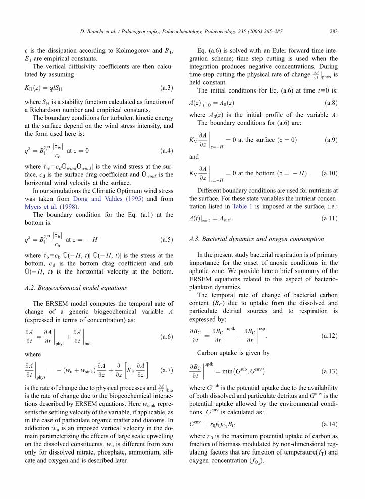
A.2. Biogeochemical model equations

The ERSEM model computes the temporal rate of

change of a generic biogeochemical variable A

(expressed in terms of concentration) as:

BA

Bt¼ BA

Bt

��phys

þ BA

Bt

��bio

ða:6Þ

where

BA

Bt

��phys

¼ � wu þ wsinkð Þ BABzþ B

BzKH

BA

Bz

��ða:7Þ

is the rate of change due to physical processes and BABtjbio

is the rate of change due to the biogeochemical interac-

tions described by ERSEM equations. Here wsink repre-

sents the settling velocity of the variable, if applicable, as

in the case of particulate organic matter and diatoms. In

addiction wu is an imposed vertical velocity in the do-

main parameterizing the effects of large scale upwelling

on the dissolved constituents. wu is different from zero

only for dissolved nitrate, phosphate, ammonium, sili-

cate and oxygen and is described later.

Eq. (a.6) is solved with an Euler forward time inte-

gration scheme; time step cutting is used when the

integration produces negative concentrations. During

time step cutting the physical rate of change BABtjphys is

held constant.

The initial conditions for Eq. (a.6) at time t=0 is:

A zð Þjt¼0 ¼ A0 zð Þ ða:8Þ

where A0(z) is the initial profile of the variable A.

The boundary conditions for (a.6) are:

KV

BA

Bz

��z¼�H

¼ 0 at the surface z ¼ 0ð Þ ða:9Þ

and

KV

BA

Bz

��z¼�H

¼ 0 at the bottom z ¼ � Hð Þ: ða:10Þ

Different boundary conditions are used for nutrients at

the surface. For these state variables the nutrient concen-

tration listed in Table 1 is imposed at the surface, i.e.:

A tð Þjz¼0 ¼ Asurf : ða:11Þ

A.3. Bacterial dynamics and oxygen consumption

In the present study bacterial respiration is of primary

importance for the onset of anoxic conditions in the

aphotic zone. We provide here a brief summary of the

ERSEM equations related to this aspect of bacterio-

plankton dynamics.

The temporal rate of change of bacterial carbon

content (BC) due to uptake from the dissolved and

particulate detrital sources and to respiration is

expressed by:

BBC

Bt¼ BBC

Bt

��uptk

� BBC

Bt

��rsp

: ða:12Þ

Carbon uptake is given by

BBC

Bt

��uptk

¼ min Gsub;Genv� �

ða:13Þ

where Gsub is the potential uptake due to the availability

of both dissolved and particulate detritus and Genv is the

potential uptake allowed by the environmental condi-

tions. Genv is calculated as:

Genv ¼ r0fTfO2BC ða:14Þ

where r0 is the maximum potential uptake of carbon as

fraction of biomass modulated by non-dimensional reg-

ulating factors that are function of temperature( fT) and

oxygen concentration ( fO2).

ig. A.1. Vertical profiles of the upwelling vertical velocity for

summer and winter. Units are 10�5 cm s�1.


fO2is parameterized with a Michaelis-Menten for-

mulation as:

fO2¼ O2

O2 þ O24ða:15Þ

where the dissolved oxygen concentration O2 is con-

sidered, and O2* is the oxygen concentration at which

metabolic functionalities are halved.

fT is written in an exponential form as:

fT ¼ QT�1010

10 ða:16Þ

where Q10 is the characteristic temperature coefficient

of bacteria and T is the temperature in 8C.Bacterial respiration (as well as respiration of all

pelagic groups) determines an oxygen consumption

expressed by the following equation:

BO2

Bt

��rsp

¼ � hBBC

Bt

��rsp

; ða:17Þ

where h is the conversion coefficient between carbon

respired and oxygen consumed.

A.4. Vertical velocity for dissolved components: open

sea upwelling

The Ionian Basin area that comprises the area of

implementation of the model is subject to a wind

system that can determine large scale upwelling/down-

welling phenomena owing to the wind stress curl

(Ekman pumping), described by the equation:

wu ¼ kk djt � stw

qf

� �ða:18Þ

where wu is the vertical velocity, stw is the wind stress, qis the seawater density and f is the Coriolis parameter.

The order of magnitude of the vertical velocity (wmax)

can be estimated by means of a scale analysis of the

former equation.

wmax ¼ O wu½ � ¼s0

Lq0f0ða:19Þ

where we chose the significant values: s0=1 dyn cm�2,

q0=1 g cm�3 and f0=10�4 s�1 for the wind stress,

density and Coriolis parameter, and L=500 km.

By a substitution of the chosen values in the equa-

tion we get the order of magnitude of wmax, equal to

10�4 cm s�1. This value can be considered an upper

limit for the wind-induced vertical velocity. By know-

ing the sign of the wind stress curl in the area of study

(Pinardi and Navarra, 1993) we can assume wmax as

positive and therefore defining upwelling processes.

We introduced in the model a vertical upwelling ve-

locity for the dissolved components, varying in depth and

time. The maximum value of this velocity has been cho-

sen equal to the half of wmax and is reached during the

winter months, when wind stress is highest according to

observations. During late summer months this value is

reduced by a factor of 10. Fig. A.1 shows the upwelling

velocity profile during the winter maximum and the

summer minimum.

A.5. Oxygen lateral advection parameterization

In the deep parts of the Mediterranean Sea, far from

deep-water formation zones, oxygen is supplied mostly

by lateral advection processes.

To simulate the input of oxygen by horizontal ad-

vection we introduced in the model a linear relaxation

term in the ERSEM prognostic equation for the dis-

solved oxygen:

BO2

Bt¼ BO2

Bt

��phys

þ BO2

Bt

��bio

þ BO2

Bt

��relax

ða:20Þ

with

BO2 tð ÞBt

��relax

¼ � r O2 tð Þ � Oinit2

ða:21Þ

where O2init is the initial (present-day) oxygen profile

and r is the relaxation coefficient, whose inverse rep-

F


resent the temporal scale of the oxygen advection pro-

cesses and is set equal to 30 days. The effect of this

equation is to drive the oxygen concentration towards

the values expressed by the initial condition. The oxy-

gen profile correction is applied to the whole water

column in the present-day simulations, in order to

model the water mass oxygenation actually observed

in the eastern Mediterranean Sea, and from the surface

to a depth of about 500 m for the simulations of the

Climatic Optimum, according to the results of Myers

et al. (1998).

References

Allen, J.I., Blackford, J.C., Radford, P.J., 1998. An 1-D vertically

resolved modelling study of the ecosystem dynamics of the

middle and southern Adriatic Sea. Journal of Marine Systems

18, 265–286.

Allen, J.I., Somerfield, P.J., Siddorn, J., 2002. Primary and bacterial

production in the Mediterranean Sea: a modeling study. Journal of

Marine Systems 33–34, 473–495.

Baretta, J.W., Ebenhon, W., Ruardij, P., 1995. The European Regional

Seas Ecosystem Model, a complex marine ecosystem model.

Netherlands Journal of Sea Research 33 (3/4), 233–246.

Baretta-Bekker, J., Baretta, J., Rasmussen, E., 1995. The microbial

food web in the European Regional Seas Ecosystem Model.


Bethoux, J.P., 1989. Oxygen consumption, new production, vertical

advection and environmental evolution in the Mediterranean Sea.

Deep-Sea Research 36, 769–781.

Blumberg, A.F., Mellor, G.L., 1987. A description of a three dimen-

sional coastal ocean circulation model. In: Heaps, N.S. (Ed.),

Three Dimensional Coastal Ocean Models. AGU, pp. 1–16.

Boldrin, A., Miserocchi, S., Rabitti, S., Turchetto, M.M., Balboni, V.,

Socal, G., 2002. Particulate matter in the southern Adriatic and

Ionian Sea: characterisation and downward fluxes. Journal of

Marine Systems 33–34, 389–410.

Bosch, H.-J., Sinninghe Damste, J.S., de Leeuw, J.W., 1998. Mo-

lecular paleontology of Eastern Mediterranean sapropels: evi-

dence for photic zone anoxia. In: Robertson, A.H.F., Emeis,

K.-C., Richter, C., Camerlenghi, A. (Eds.), Proc. ODP Sci.

Res., vol. 160. Ocean Drilling Program, College Station, TX,

pp. 285–295.

Boyd, P.W., Newton, P.P., 1999. Does planktonic community struc-

ture determine downward particulate organic carbon flux in dif-

ferent oceanic provinces? Deep Sea Research I 46, 63–91.

Boyd, P.W., Sherry, N.D., Berges, J.A., Bishop, J.K.B., Calvert, S.E.,

Charette, M.A., Giovannoni, S.J., Goldblatt, R., Harrison, P.J.,

Moran, S.B., Roy, S., Soon, M., Strom, S., Thibault, D., Vergin,

K.L., Whitney, F.A., Wong, C.S., 1999. Transformations of bio-

genic particulates from the pelagic to the deep ocean realm. Deep

Sea Research II 46, 2761–2792.

Bregant, D., Catalano, C., Civitarese, G., Luchetta, A., 1990. Some

characteristics of the brines in Bannock and Tyro Basins: salinity,

sulphur compounds, Ca, F, pH, At, PO4, SiO2, NH3. Marine

Chemistry 31, 35–62.

Broekhuizen, N.R., Heath, M.R., Hay, S.J., Gurney, W.S.C., 1995.

Modelling the dynamics of the North Seas mesozooplankton.


Calvert, S.E., 1983. Geochemistry of Pleistocene sapropels and asso-

ciated sediments from the eastern Mediterranean. Oceanologica

Acta 6, 255–267.

Calvert, S.E., Nielsen, B., Fontugne, M.R., 1992. Evidence from

nitrogen isotope ratios for enhanced productivity during formation

of eastern Mediterranean sapropels. Nature 359, 223–225.

Casford, J.S.L., Rohling, E.J., Abu-Zied, R.H., Fontanier, C., Joris-

sen, F., Leng, J., Schmiedl, M.J., Thomson, G., 2003. A dynamic

concept for eastern Mediterranean circulation and oxygenation

during sapropel formation. Palaeogeography, Palaeoclimatology,

Palaeoecology 190, 103–119.

Casotti, R., Landolfi, A., Brunet, C., D’Ortenzio, F., Mangoni, O.,

Ribera D’Alcala, M., 2003. Composition and dynamics of the

phytoplankton of the Ionian Sea (eastern Mediterranean). Journal

of Geophysical Research 108 (PBE 17-1/17-19).

Castradori, D., 1993. Calcareous nannofossils and the origin of

eastern Mediterranean sapropels. Paleoceanography 8, 459–472.

Cita, M.B., Vergnaud-Grazzini, C., Robert, C., Chamley, H., Ciaranfi,

N., D’Onofrio, S., 1977. Paleoclimatic record of a long deep sea

core from the eastern Mediterranean. Quaternary Research 8,

205–235.

Cramp, A., O’Sullivan, G., 1999. Neogene sapropel in the Mediter-

ranean: a review. Marine Geology 153, 11–28.

Da Silva, A.M., Young, C.C., Levitus, S., 1995. Atlas of surface

marine data. NOAA Atlas NESDIS, 7.

De Rijk, S., Hayes, A., Rohling, E.J., 1999. Eastern Mediterra-

nean sapropel S1 interruption: an expression of the onset of

climatic deterioration around 7 ka BP. Marine Geology 153,

337–343.

Dong, B., Valdes, P.J., 1995. Sensitivity studies of northern hemi-

sphere glaciation using an atmosphere GCM. Journal of Climate

8, 2471–2496.

Druon, J.N., Le Fevre, J.L., 1999. Sensitivity of a pelagic ecosystem

model to variations of process parameters within a realistic range.

Journal of Marine Systems 19, 1–26.

Ebenhoh, W., Kohlmier, C., Radford, P., 1995. The benthic biological

submodel in the European Regional Seas Ecosystem Model.


Ediger, D., Yilmaz, A., 1996. Characteristics of deep chlorophyll

maximum in the Northeastern Mediterranean with respect

to environmental conditions. Journal of Marine Systems 9,

291–303.

Emeis, K.-C., Sakamoto, T., Wehausen, R., Brumsack, H.-J., 2000.

The sapropel record of the eastern Mediterranean Sea—results of

Ocean Drilling Program Leg 160. Palaeogeography, Palaeoclima-

tology, Palaeoecology 158, 371–395.

Harris, J.R.W., Stutt, E.D., Turley, C.M., 2001. Carbon flux in the

northwest Mediterranean estimated from microbial production.

Deep-Sea Research I 48, 2631–2644.

Hartnett, H.E., Keil, R.G., Hedges, J.I., Devol, A.H., 1998. Influence

of oxygen exposure time on organic carbon preservation in con-

tinental margin sediments. Nature 391, 572–574.

Hilgen, F.J., 1991. Astronomical calibration of Gauss to Matuyama

sapropels in the Mediterranean and implication for the Geomag-

netic Polarity Time Scale. Earth and Planetary Science Letters

104, 226–244.

Hodges, B.A., Rudnick, D.L., 2004. Simple models of steady deep

maxima in chlorophyll and biomass. Deep-Sea Research I 51,

999–1015.

Honjo, S., Manganini, S.J., 1993. Annual biogenic particle fluxes to

the interior of the North Atlantic Ocean; studied at 348N 218Wand 488N 218W. Deep-Sea Research II 40, 587–607.


Honjo, S., Dymond, J., Collier, R., Manganini, S.J., 1995. Export

production of particles to the interior of the equatorial Pacific

Ocean during the 1992 EqPac experiment. Deep-Sea Research

Part II 42, 831–870.

Howell, M.W., Thunnell, R.C., 1992. Organic carbon accumulation in

Bannock Basin: evaluating the role of productivity in the forma-

tion of eastern Mediterranean sapropels. Marine Geology 103,

461–471.

Ignatiades, L., Psarra, S., Zervakis, V., Pagou, K., Souvermezoglou,

E., Assimakopoulou, G., Gotsis-Skretas, O., 2002. Phytoplankton

size-based dynamics in the Aegean Sea (Eastern Mediterranean).

Journal of Marine Systems 36, 11–28.

Jorissen, F.J., 1999. Benthic foraminiferal succession across Late

Quaternary Mediterranean sapropels. Marine Geology 153,

91–101.

Kallel, N., Paterne, M., Duplessy, J., Vergnaud-Grazzini, C., Pujol, C.,

Labeyrie, L., Arnold, M., Fontugne, M.R., Pierre, C., 1997.

Enhanced rainfall in the Mediterranean region during the last

sapropel event. Oceanologica Acta 20, 697–712.

Kemp, A.E.S., Pearce, R.B., Koizumi, I., Pike, J., Rance, S.J., 1999.

The role of mat-forming diatoms in the formation of Mediterra-

nean sapropels. Nature 398, 57–61.

Kidd, R.B., Cita, M.B., Ryan, W.B.F., 1978. Stratigraphy of eastern

Mediterranean sapropel sequences recovered during DSDP Leg

42A and their paleoenvironmental significance. Initial Reports of

the Deep Sea Drilling Project 42, 421–443.

Krom, M.D., Michard, A., Cliff, R., Strohle, A., 1999. Source of

sediments to the Ionian Sea and western Levantine basin of the

eastern Mediterranean during S-1 sapropel times. Marine Geology

160, 45–61.

Kroon, D., Alexander, I., Little, M., Lourens, L.J., Matthewson, A.,

Robertson, A.H.F., Sakamoto, T., 1998. Oxygen isotope and

sapropel stratigraphy in the eastern Mediterranean during the

last 3.2 million years. Proceedings of the Ocean Drilling Program,

Scientific Results 160, 181–189.

Larrasoana, J.C., Roberts, A.P., Rohling, E.J., Winklhofer, M.,

Wehausen, R., 2003. Three million years of monsoon variability

over the northern Sahara. Climate Dynamics 21, 689–698.

Li, W.K.W., Suba-Rao, D.V., Harrison, W.G., Smith, J.C., Cullen, J.J.,

Irwin, B., Platt, T., 1983. Autotrophic picoplankton in the tropical

ocean. Science 219, 292–295.

Magazzu, G., Decembrini, F., 1995. Primary production, biomass and

abundance of phototrophic picoplankton in the Mediterranean

Sea: a review. Aquatic Microbial Ecology 9, 97–104.

Martinez-Ruiz, F., Kastner, M., Paytan, A., Ortega-Huertas, M., Ber-

nasconi, S.M., 2000. Geochemical evidence for enhanced produc-

tivity during S1 sapropel deposition in the eastern Mediterranean.

Paleoceanography 15, 200–209.

Martinez-Ruiz, F., Paytan, A., Kastner, M., Gonzales-Donoso, J.M.,

Linares, D., Bernasconi, S.M., Jimenez-Espejo, F.J., 2003. A

comparative study of the geochemical and mineralogical charac-

teristics of the S1 sapropel in the western and eastern Mediterra-

nean. Palaeogeography, Palaeoclimatology, Palaeoecology 190,

23–37.

Mellor, G.L., Yamada, T., 1982. Development of a turbulence closure

model for geophysical fluid problems. Review of Geophysics and

Space Physics 20, 851–875.

Mercone, D., Thomson, J., Croudace, I.W., Siani, G., Paterne, M.,

Troelstra, S., 2000. Duration of S1, the most recent sapropel in the

eastern Mediterranean Sea, as indicated by accelerator mass spec-

trometry radiocarbon and geochemical evidence. Paleoceanogra-

phy 15, 336–347.

Moutin, T., Rainbault, P., 2002. Primary production, carbon export

and nutrient availability in western and eastern Mediterranean Sea

in early summer 1996 (MINOS cruise). Journal of Marine Sys-

tems 33–34, 273–288.

Murat, A., Got, H., 2000. Organic carbon variations of the eastern

Mediterranean Holocene sapropel: a key for understanding for-

mation processes. Palaeogeography, Palaeoclimatology, Palaeoe-

cology 158, 241–257.

Myers, P.G., Haines, K., Rohling, E.J., 1998. Modelling the paleo-

circulation of the Mediterranean: the last glacial maximum and the

Holocene with emphasis on the formation of Sapropel S1. Paleo-

ceanography 13, 586–606.

Olausson E., 1961. Studies of deep-sea cores: Reports of the Swedish

Deep-Sea Expedition, 1947–1948, 8, 323–438.

Passier, H.F., Middelburg, J.J., De Lange, G.J., Bottcher, M.E.,

1999a. Modes of sapropel formation in the eastern Mediterra-

nean: some constraints based on pyrite properties. Marine Geol-

ogy 153, 199–219.

Passier, H.F., Bosch, H.J., Nijenhuis, I.A., Lourens, L.J., Bottcher,

M.E., Leenders, A., Sinninghe Damste, J.S., De Lange, G.J.,

Leeuw, J.W., 1999b. Sulphic Mediterranean surface waters during

Pliocene sapropel formation. Nature 397, 146–149.

Pearce, R.B., Kemp, A.E.S., Koizumi, I., Pike, J., Cramp, A., Row-

land, S.J., 1998. A lamina-scale SEM-based study of a late

Quaternary diatom-ooze sapropel from the Mediterranean ridge,

site 971. In: Robertson, A.H.F., Emeis, K.-C., Richter, C., Camer-

lenghi, A. (Eds.), Proc. ODP Sci. Res., vol. 160. Ocean Drilling

Program, College Station, TX, pp. 349–363.

Pedersen, T.F., Calvert, S.E., 1990. Anoxia vs. productivity: what

controls the formation of organic-carbon-rich sediments and sed-

imentary rocks? AAPG Bullettin 74, 454–466.

Pinardi, N., Navarra, A., 1993. Baroclinic wind adjustment pro-

cesses in the Mediterranean Sea. Deep-Sea Research Part II 40,

1299–1326.

Pinardi, N., Zavatarelli, M., Arnieri, E., Crise, A., Ravaioli, M., 2005.

The physical, sedimentary and ecological structure and variability

of shelf areas in the Mediterranean Sea Chapter 32. Robinson,

A.R., Brink, K.H. (Eds.), The Sea, vol. 14. Harvard University

Press, pp. 1243–1330.

Rabitti, S., Bianchi, F., Boldrin, A., Ros, L.D., Socal, G., Totti, C.,

1994. Particulate matter and phytoplankton in the Ionian Sea.

Oceanologica Acta 17, 297–307.

Redfield, A.C., Ketchum, B.H., Richards, F.A., 1963. The influence

of organisms on the composition of seawater. In: Hill, M.N. (Ed.),

The Sea, vol. 2. Interscience, New York, pp. 26–77.

Roether, W., Klein, B., Bregant, D., Georgopoulos, D., Beitzel, V.,

Kovacevich, V., Lucchetta, A., 1996. Recent changes in eastern

Mediterranean deep waters. Science 271, 333–335.

Rohling, E.J., 1994. Review and new aspects concerning the

formation of eastern Mediterranean sapropels. Marine Geology

122, 1–28.

Rohling, E.J., Gieskes, W.W.C., 1989. Late Quaternary changes in

Mediterranean intermediate water density and formation rate.

Paleoceanography 4, 531–545.

Rohling, E.J., Jorissen, F.J., De Stigter, H.C., 1997. 200 years inter-

ruption of Holocene sapropel formation in the Adriatic Sea.

Journal of Micropaleontolology 16 (2), 97–108.

Rohling, E.J., Cane, T.R., Cooke, S., Sprovieri, M., Bouloubassi, I.,

Emeis, K.C., Schiebel, R., Kroon, D., Jorissen, F.J., Lorre, A.,

Kemp, A.E.S., 2002. African monsoon variability during the

previous interglacial maximum. Earth and Planetary Science Let-

ters 202, 61–75.


Rossignol-Strick, M., 1983. African monsoons, an immediate climate

response to orbital insolation. Nature 304, 46–49.

Rossignol-Strick, M., 1985. Mediterranean Quaternary sapropels: an

immediate response of the African monsoon to variation of inso-

lation. Palaeogeography, Palaeoclimatology, Palaeoecology 49,

237–265.

Ruardij, P., Van Raaphorst, W., 1995. Benthic nutrient regeneration in

the ERSEM ecosystem model of the North Sea. Netherlands

Journal of Sea Research 33 (3/4), 453–483.

Sachs, J.P., Repeta, D.J., 1999. Oligotrophy and nitrogen fixation

during eastern Mediterranean sapropel events. Science 286,

2485–2488.

Slomp, C.P., Thomson, J., De Lange, G.J., 2004. Controls on phos-

phorus regeneration and burial during formation of eastern Med-

iterranean sapropels. Marine Geology 203, 141–159.

Smith, C.R., Hoover, D.J., Doan, S.E., Pope, R.H., Demaster, D.J.,

Dobbs, F.C., Altabet, M.A., 1996. Phytodetritus at the abyssal

seafloor across 108 of latitude in the central equatorial Pacific.

Deep-Sea Research II 43, 1309–1338.

Stratford, K., Williams, R.G., Myers, P.G., 2000. Impact of the

circulation on sapropel formation in the eastern Mediterranean.

Global Biogeochemical Cycles 14, 685–695.

Strohle, K., Krom, M.D., 1997. Evidence for the evolution for an

oxygen minimum layer at the beginning of S-1 sapropel deposi-

tion in the eastern Mediterranean. Marine Geology 140, 231–236.

Van Santvoort, P.J.M., De Lange, G.J., Langereis, C.G., Dekkers,

M.J., Paterne, M., 1997. Geochemical and paleomagnetic evi-

dence for the occurrence of bmissingQ sapropels in eastern Med-

iterranean sediments. Paleoceanography 12, 773–786.

Varela, R.A., Cruzado, A., Gabaldon, J.E., 1995. Modelling primary

production in the North Sea using the European Regional Seas

Ecosystem Model. Netherlands Journal of Sea Research 33 (3/4),

441–463.

Vergnaud-Grazzini, C., Ryan, W.B.F., Cita, M.B., 1977. Stable iso-

tope fractionation, climate change and episodic stagnation in the

eastern Mediterranean Pleistocene records. Marine Micropaleon-

tology 10, 35–69.

Vichi, M., Oddo, P., Zavatarelli, M., Coluccelli, A., Coppini, G.,

Celio, M., Fonda Umani, S., Pinardi, N., 2003. Calibration and

validation of a one-dimensional complex marine biogeochemical

flux model in different areas of the northern Adriatic shelf.

Annales Geophysicae 21, 413–436.

Warning, B., Brumsack, H.J., 2000. Trace metal signatures of eastern

Mediterranean sapropels. Palaeogeography, Palaeoclimatology,

Palaeoecology 158, 293–309.

Wehausen, R., Brumsack, H.J., 1999. Cyclic variations in the chem-

ical composition of eastern Mediterranean Pliocene sediments: a

key for understanding sapropel formation. Marine Geology 153,

161–176.

Weldeab, S., Emeis, K.C., Hemleben, C., Schmiedl, G., Schulz, H.,

2003. Spatial productivity variations during formation of sapro-

pels s5 and s6 in the Mediterranean Sea: evidence from Ba

contents. Palaeogeography, Palaeoclimatology, Palaeoecology

191, 169–190.

Zavatarelli, M., Raicich, M., Bregant, D., Russo, A., Artegiani, A.,

1998. Climatological biogeochemical characteristics of the Adria-

tic Sea. Journal of Marine Systems 18, 227–263.

Simulations of ecosystem response during the sapropel S1 deposition event

Documents

Transcript of Simulations of ecosystem response during the sapropel S1 deposition event