simulation of interlaminar and intralaminar damage in polymer ...
328
SIMULATION OF INTERLAMINAR AND INTRALAMINAR DAMAGE IN POLYMER-BASED COMPOSITES FOR AERONAUTICAL APPLICATIONS UNDER IMPACT LOADING Emilio Vicente GONZÁLEZ JUAN ISBN: 978-84-694-4282-1 Dipòsit legal: GI-695-2011 http://hdl.handle.net/10803/22834 ADVERTIMENT. La consulta d’aquesta tesi queda condicionada a l’acceptació de les següents condicions d'ús: La difusió d’aquesta tesi per mitjà del servei TDX ha estat autoritzada pels titulars dels drets de propietat intel·lectual únicament per a usos privats emmarcats en activitats d’investigació i docència. No s’autoritza la seva reproducció amb finalitats de lucre ni la seva difusió i posada a disposició des d’un lloc aliè al servei TDX. No s’autoritza la presentació del seu contingut en una finestra o marc aliè a TDX (framing). Aquesta reserva de drets afecta tant al resum de presentació de la tesi com als seus continguts. En la utilització o cita de parts de la tesi és obligat indicar el nom de la persona autora. ADVERTENCIA. La consulta de esta tesis queda condicionada a la aceptación de las siguientes condiciones de uso: La difusión de esta tesis por medio del servicio TDR ha sido autorizada por los titulares de los derechos de propiedad intelectual únicamente para usos privados enmarcados en actividades de investigación y docencia. No se autoriza su reproducción con finalidades de lucro ni su difusión y puesta a disposición desde un sitio ajeno al servicio TDR. No se autoriza la presentación de su contenido en una ventana o marco ajeno a TDR (framing). Esta reserva de derechos afecta tanto al resumen de presentación de la tesis como a sus contenidos. En la utilización o cita de partes de la tesis es obligado indicar el nombre de la persona autora. WARNING. On having consulted this thesis you’re accepting the following use conditions: Spreading this thesis by the TDX service has been authorized by the titular of the intellectual property rights only for private uses placed in investigation and teaching activities. Reproduction with lucrative aims is not authorized neither its spreading and availability from a site foreign to the TDX service. Introducing its content in a window or frame foreign to the TDX service is not authorized (framing). This rights affect to the presentation summary of the thesis as well as to its contents. In the using or citation of parts of the thesis it’s obliged to indicate the name of the author.
-
Upload
khangminh22 -
Category
Documents
-
view
5 -
download
0
Transcript of simulation of interlaminar and intralaminar damage in polymer ...

SIMULATION OF INTERLAMINAR AND INTRALAMINAR DAMAGE IN POLYMER-BASED
COMPOSITES FOR AERONAUTICAL APPLICATIONS UNDER IMPACT LOADING
Emilio Vicente GONZÁLEZ JUAN
ISBN: 978-84-694-4282-1 Dipòsit legal: GI-695-2011 http://hdl.handle.net/10803/22834
ADVERTIMENT. La consulta d’aquesta tesi queda condicionada a l’acceptació de les següents condicions d'ús: La difusió d’aquesta tesi per mitjà del servei TDX ha estat autoritzada pels titulars dels drets de propietat intel·lectual únicament per a usos privats emmarcats en activitats d’investigació i docència. No s’autoritza la seva reproducció amb finalitats de lucre ni la seva difusió i posada a disposició des d’un lloc aliè al servei TDX. No s’autoritza la presentació del seu contingut en una finestra o marc aliè a TDX (framing). Aquesta reserva de drets afecta tant al resum de presentació de la tesi com als seus continguts. En la utilització o cita de parts de la tesi és obligat indicar el nom de la persona autora. ADVERTENCIA. La consulta de esta tesis queda condicionada a la aceptación de las siguientes condiciones de uso: La difusión de esta tesis por medio del servicio TDR ha sido autorizada por los titulares de los derechos de propiedad intelectual únicamente para usos privados enmarcados en actividades de investigación y docencia. No se autoriza su reproducción con finalidades de lucro ni su difusión y puesta a disposición desde un sitio ajeno al servicio TDR. No se autoriza la presentación de su contenido en una ventana o marco ajeno a TDR (framing). Esta reserva de derechos afecta tanto al resumen de presentación de la tesis como a sus contenidos. En la utilización o cita de partes de la tesis es obligado indicar el nombre de la persona autora. WARNING. On having consulted this thesis you’re accepting the following use conditions: Spreading this thesis by the TDX service has been authorized by the titular of the intellectual property rights only for private uses placed in investigation and teaching activities. Reproduction with lucrative aims is not authorized neither its spreading and availability from a site foreign to the TDX service. Introducing its content in a window or frame foreign to the TDX service is not authorized (framing). This rights affect to the presentation summary of the thesis as well as to its contents. In the using or citation of parts of the thesis it’s obliged to indicate the name of the author.

Universitat de Girona
PhD Thesis
Simulation of interlaminar and
intralaminar damage in
polymer-based composites for
aeronautical applications under
impact loading
Emilio Vicente Gonzalez Juan
2010

Universitat de Girona
PhD Thesis
Simulation of interlaminar and
intralaminar damage in polymer-based
composites for aeronautical
applications under impact loading
Emilio Vicente Gonzalez Juan
2010
Technology Doctorate Program
Advisors
Dr. Pere Maimı Vert Dr. Pedro P. Camanho
Universitat de Girona, Spain Universidade do Porto, Portugal
A thesis submitted for the degree of Doctor of Philosophy by the
University of Girona
To whom it might concern,
Dr. Pere Maimı Vert, Associate Professor at the Universitat de Girona of the
Department of Enginyeria Mecanica i de la Construccio Industrial, and Dr. Pedro
Manuel Ponces Rodrigues de Castro Camanho, Associate Professor at the Univer-
sidade do Porto of the Department of Engenharia Mecanica,
CERTIFY that the study entitled Simulation of interlaminar and intralaminar dam-
age in polymer-based composites for aeronautical applications under impact loading
has been carried out under their supervision by Emilio Vicente Gonzalez Juan to
apply the doctoral degree with the European Mention,
Girona, October 2010,
Dr. Pere Maimı Vert Dr. Pedro P. Camanho
Universitat de Girona, Spain Universidade do Porto, Portugal

A mis padres,
Angel y Tere

Acknowledgements - Agraıments - Agradecimien-tos
I would like to express my most sincerely gratitude to my advisors, Pere Maimı and
Pedro P. Camanho, for the indefatigable help and for the key contributions that
have allowed the development of the present thesis. I feel very fortunate to have
worked with them. The treatment that I have received since the first day has been
close and friendly, and this good relationship has grown day by day yielding to a
nice friendship and allowing to enjoy a lot with the work.
I want to thank also the help received from Joan Andreu Mayugo, Josep Costa
and Norbert Blanco, who have spent a lot of time making the work easy and clar-
ifying a lot of things, not only related to composite materials, also in many other
things which are required to continue forward. This help has existed always, since
the first day that I started to work with the research group AMADE in July of
2003. Also, I have to remember that they are the guilty of encouraged me to start
the thesis.
I have to do a special mention of my friends G. Catalanotti, C.S. Lopes, and H.
Koerber, with the ones that I have shared great moments and I have learned a lot
of them during my research stages at the University of Porto. In addition, I would
like to express my gratitude to Carlos Davila who offered me the possibility to visit
NASA - Langley Research Center in Hampton, during the summer of 2008.
Of course, I am grateful to all members of the research group AMADE of the
University of Girona for the help and nice moments that I have received from each
one: A. Turon, J. Renart, D. Trias, M. Baena, M. Gascons, P. Vicens, E. Pajares,
R. Cruz, J. Bonilla, C. Mias, Ll. Ripoll, L. Zubillaga, N. Isart, S. Ortiz, C. Barris,
I. Vilanova, D. Sans, J. Bofill, P. Badallo, T. Kanzaki, N. Gascons, J. Torres, Ll.
Torres, J. Vives and M. Compte. In addition, I want to thank to: Grup de Recerca
en Enginyeria de Producte, Proces i Produccio (GREP), of the University of Girona,
in special to Jordi Delgado, for the dent-depth measurements; Instituto Nacional de
Tecnica Aeroespacial (INTA), for the help in the specimen manufacturing; Mechanic
Engineering Laboratory of the University of Porto for the manufacturing of the test
rigs; and the Computer Science team of INEGI (University of Porto) for the well
working of the cluster for the computation of the simulations.

No vull oblidar els meus amics, Aniceto, Auguet, Blai, Calli, Manel·la, Palacios,
i Terri, pels bons moments de desconnexio que m’heu donat, encara que no han
pogut ser molts, pero que han estat intensos i divertits.
Finalmente, quiero dar un especial agradecimiento a mi hermana Bego, mi
cunado Joan, y a mis padres, Angel y Tere, por la confianza, apoyo y animos que
me habeis dado, no solo en este proyecto, sino a lo largo de mi vida para todas las
dificultades que se me han presentado. Estoy en deuda con vosotros.

Funds
The period of doctorate studies comprised between July of 2006 and June of 2007 has
been supported by the University of Girona through the research grant BR06/07.
The period of research has been funded by the Comissionat per a Universitats i
Recerca del Departament d’Innovacio, Universitats i Empresa de la Generalitat de
Catalunya, and by European Social Funds, under a research grant FI - Formacio de
Personal Investigador, started in July of 2007 and finished in June of 2010.
Also, the present work has been partially funded by the Spanish Government
through the contracts MAT2006-14159-C02-01 and TRA2006-15718-C02-01/TAIR,
and by the Portuguese Foundation for Science and Technology under the project
PDCT/EMEPME/64984/2006.
Part of the work has been carried out during three stages at the University of
Porto, under the grants for mobility: VUDG-2007 (of the University of Girona),
and BE-2008 and BE-2009 (of the Comissionat per a Universitats i Recerca del
Departament d’Innovacio, Universitats i Empresa de la Generalitat de Catalunya).
Also, the analysis of some topics were performed during the research stage at NASA
- Langley Research Center in Hampton (Virginia, USA), that was supported by the
National Institute of Aerospace (NIA), in the summer of 2008.
Finally, I want to thank the award received in May of 2009 for the best thesis
project, announced by the Associacio d’Enginyers Industrials de Catalunya, and
supported by the Agrupacio Socio-Cultural dels Enginyers Industrials de Catalunya.
Resumen
La aplicacion de materiales compuestos de matriz polimerica reforzados mediante
fibras largas (FRP, ”Fiber Reinforced Plastic”), esta en gradual crecimiento debido
a las buenas propiedades especıficas y a la flexibilidad en el diseno. Uno de los
mayores consumidores es la industria aeroespacial, dado que la aplicacion de estos
materiales tiene claros beneficios economicos y medioambientales.
Cuando los materiales compuestos se aplican en componentes estructurales, se
inicia un programa de diseno donde se combinan ensayos reales y tecnicas de analisis.
El desarrollo de herramientas de analisis fiables que permiten comprender el com-
portamiento mecanico de la estructura, ası como reemplazar muchos, pero no todos,
los ensayos reales, es de claro interes.
Susceptibilidad al dano debido a cargas de impacto fuera del plano es uno de los
aspectos de mas importancia que se tienen en cuenta durante el proceso de diseno
de estructuras de material compuesto. La falta de conocimiento de los efectos del
impacto en estas estructuras es un factor que limita el uso de estos materiales.
Por lo tanto, el desarrollo de modelos de ensayo virtual mecanico para analizar
la resistencia a impacto de una estructura es de gran interes, pero aun mas, la
prediccion de la resistencia residual despues del impacto.
En este sentido, el presente trabajo abarca un amplio rango de analisis de eventos
de impacto a baja velocidad en placas laminadas de material compuesto, monolıticas,
planas, rectangulares, y con secuencias de apilamiento convencionales. Teniendo en
cuenta que el principal objetivo del presente trabajo es la prediccion de la resistencia
residual a compresion, diferentes tareas se llevan a cabo para favorecer el adecuado
analisis del problema. Los temas que se desarrollan son: la descripcion analıtica
del impacto, el diseno y la realizacion de un plan de ensayos experimentales, la
formulacion e implementacion de modelos constitutivos para la descripcion del com-
xi

xii RESUMEN
portamiento del material, y el desarrollo de ensayos virtuales basados en modelos
de elementos finitos en los que se usan los modelos constitutivos implementados.

Summary
The application of polymer-based composites reinforced by long fibers, called ad-
vanced Fiber Reinforced Plastic (FRP), is gradually increasing as a result of their
good specific mechanical properties and increased flexibility of design. One of the
largest consumers is the aerospace industry, since the application of these materials
has clear economic and environmental benefits.
When composites are to be used in structural components, a design develop-
ment program is initiated, where a combination of testing and analysis techniques
is typically performed. The development of reliable analysis tools that enable to
understand the structure mechanical behavior, as well as to replace most, but not
all, the real experimental tests, is of clear interest.
Susceptibility to damage from concentrated out-of-plane impact forces is one
of the major design concerns of structures made of advanced FRPs used in the
aerospace industry. Lack of knowledge of the impact effects on these structures is a
factor in limiting the use of composite materials.
Therefore, the development of virtual mechanical testing models to analyze the
impact damage resistance of a structure is of great interest, but even more, the
prediction of the post-impact residual strength.
In this sense, the present thesis covers a wide range of analysis of the low-
velocity and large mass impact events on monolithic, flat, rectangular, polymer-
based laminated composite plates with conventional stacking sequences. Keeping in
mind that the main goal of this work is the prediction of the residual compressive
strength of an impacted specimen coupon, a set of different tasks are performed in
order to provide suitable tools to analyze the problem. Accordingly, the topics which
are addressed in this thesis are: the analytical description of the impact, the design
and the realization of an experimental test plan, the formulation and implementation
xiii

xiv SUMMARY
of constitutive models for the description of the composite material behavior, and
the assessment of the performance of virtual tests based on finite element models
where the constitutive models are used.

Contents
Resumen xi
Summary xiii
List de Figures xxvii
List de Tables xxx
List of Symbols xxxi
List of Acronyms xlvii
1 Introduction and objectives 1
1.1 Introduction . . . . . . . . . . . . . . . . . . . . . . . . . . . . . . . . 1
1.2 Motivation . . . . . . . . . . . . . . . . . . . . . . . . . . . . . . . . . 4
1.3 Objectives . . . . . . . . . . . . . . . . . . . . . . . . . . . . . . . . . 5
1.4 Thesis lay-out . . . . . . . . . . . . . . . . . . . . . . . . . . . . . . . 6
2 Analytical description of the impact event 9
2.1 Introduction . . . . . . . . . . . . . . . . . . . . . . . . . . . . . . . . 9
2.2 Impact behavior . . . . . . . . . . . . . . . . . . . . . . . . . . . . . . 10
2.3 Local deflection . . . . . . . . . . . . . . . . . . . . . . . . . . . . . . 13
2.3.1 Hertz contact law adapted for laminated composite plates . . 16
2.3.2 Unloading and reloading contact process . . . . . . . . . . . . 18
2.3.3 Elastic-plastic contact models . . . . . . . . . . . . . . . . . . 20
2.3.4 Linearized contact laws . . . . . . . . . . . . . . . . . . . . . . 22
2.4 Analytical impact models . . . . . . . . . . . . . . . . . . . . . . . . 22
xv

xvi CONTENTS
2.4.1 Complete analytical models . . . . . . . . . . . . . . . . . . . 24
2.4.2 Infinite plate impact models . . . . . . . . . . . . . . . . . . . 29
2.4.3 Half-space impact models . . . . . . . . . . . . . . . . . . . . 35
2.4.4 Quasi-static impact models . . . . . . . . . . . . . . . . . . . 36
2.5 Approaches for impact behavior description . . . . . . . . . . . . . . 38
2.5.1 Christoforou and Yigit characterization diagram . . . . . . . . 38
2.5.2 Olsson mass criterion . . . . . . . . . . . . . . . . . . . . . . . 42
2.6 Impact damage and analytical thresholds . . . . . . . . . . . . . . . . 45
2.6.1 Matrix cracking . . . . . . . . . . . . . . . . . . . . . . . . . . 45
2.6.2 Delamination . . . . . . . . . . . . . . . . . . . . . . . . . . . 51
2.6.3 Permanent indentation . . . . . . . . . . . . . . . . . . . . . . 57
2.6.4 Fiber failure . . . . . . . . . . . . . . . . . . . . . . . . . . . . 58
2.6.5 Perforation . . . . . . . . . . . . . . . . . . . . . . . . . . . . 58
3 Test configurations 61
3.1 Introduction . . . . . . . . . . . . . . . . . . . . . . . . . . . . . . . . 61
3.2 Impact tests . . . . . . . . . . . . . . . . . . . . . . . . . . . . . . . . 62
3.2.1 Benchmark: ASTM drop-weight impact test . . . . . . . . . . 63
3.2.2 Selected studies: fixed and variable parameters . . . . . . . . . 67
3.3 Compression after impact tests (CAI) . . . . . . . . . . . . . . . . . . 78
3.3.1 Benchmark: ASTM compression after impact test . . . . . . . 79
3.3.2 Resources used and specimen instrumentation . . . . . . . . . 81
4 Experimental results 83
4.1 Introduction . . . . . . . . . . . . . . . . . . . . . . . . . . . . . . . . 83
4.2 Effect of ply thickness (clustering) . . . . . . . . . . . . . . . . . . . . 84
4.2.1 Impact tests . . . . . . . . . . . . . . . . . . . . . . . . . . . . 84
4.2.2 NDI: C-scan after impact . . . . . . . . . . . . . . . . . . . . . 91
4.2.3 Dent-depth measurements . . . . . . . . . . . . . . . . . . . . 96
4.2.4 CAI tests . . . . . . . . . . . . . . . . . . . . . . . . . . . . . 97
4.3 Effect of ply mismatch angle at interfaces . . . . . . . . . . . . . . . . 103
4.3.1 Impact tests . . . . . . . . . . . . . . . . . . . . . . . . . . . . 103
4.3.2 NDI: C-scan after impact . . . . . . . . . . . . . . . . . . . . . 108
4.3.3 Dent-depth measurements . . . . . . . . . . . . . . . . . . . . 110

CONTENTS xvii
4.3.4 CAI tests . . . . . . . . . . . . . . . . . . . . . . . . . . . . . 111
4.4 Effect of the laminate thickness . . . . . . . . . . . . . . . . . . . . . 113
4.4.1 Impact tests . . . . . . . . . . . . . . . . . . . . . . . . . . . . 113
4.4.2 NDI: C-scan after impact . . . . . . . . . . . . . . . . . . . . . 123
4.4.3 Dent-depth measurements . . . . . . . . . . . . . . . . . . . . 127
4.4.4 CAI tests . . . . . . . . . . . . . . . . . . . . . . . . . . . . . 128
4.5 Summary of conclusions . . . . . . . . . . . . . . . . . . . . . . . . . 133
5 Interlaminar damage model 137
5.1 Introduction . . . . . . . . . . . . . . . . . . . . . . . . . . . . . . . . 137
5.2 Damage model formulation . . . . . . . . . . . . . . . . . . . . . . . . 141
5.2.1 Norm of the relative displacement vector . . . . . . . . . . . . 143
5.2.2 Surface of damage activation and law for damage evolution . . 144
5.2.3 Criterion for damage propagation . . . . . . . . . . . . . . . . 145
5.2.4 Criterion for damage onset . . . . . . . . . . . . . . . . . . . . 147
5.3 Formulation adaptations . . . . . . . . . . . . . . . . . . . . . . . . . 148
5.3.1 Relation between relative displacements and strains . . . . . . 148
5.3.2 Penalty stiffness . . . . . . . . . . . . . . . . . . . . . . . . . . 149
5.3.3 Redefined onset and propagation damage criteria . . . . . . . 150
5.4 Model implementation . . . . . . . . . . . . . . . . . . . . . . . . . . 153
5.4.1 Strategy of implementation . . . . . . . . . . . . . . . . . . . 153
5.4.2 Input variables to define the model . . . . . . . . . . . . . . . 154
5.4.3 Algorithm . . . . . . . . . . . . . . . . . . . . . . . . . . . . . 156
5.5 Size of cohesive elements . . . . . . . . . . . . . . . . . . . . . . . . . 159
5.5.1 Maximum thickness of volumetric cohesive elements . . . . . . 159
5.5.2 In-plane dimensions of the cohesive elements . . . . . . . . . . 161
5.6 Simulations . . . . . . . . . . . . . . . . . . . . . . . . . . . . . . . . 162
5.6.1 Considerations for quasi-static explicit simulations . . . . . . . 163
5.6.2 MMB and ENF fracture toughness tests . . . . . . . . . . . . 164
5.6.3 TCT tests . . . . . . . . . . . . . . . . . . . . . . . . . . . . . 171
5.7 Conclusions . . . . . . . . . . . . . . . . . . . . . . . . . . . . . . . . 174
6 Intralaminar damage model 177
6.1 Introduction . . . . . . . . . . . . . . . . . . . . . . . . . . . . . . . . 177

xviii CONTENTS
6.2 Continuum damage model . . . . . . . . . . . . . . . . . . . . . . . . 178
6.2.1 Constitutive model . . . . . . . . . . . . . . . . . . . . . . . . 178
6.2.2 Damage activation functions . . . . . . . . . . . . . . . . . . . 180
6.2.3 Damage evolution laws . . . . . . . . . . . . . . . . . . . . . . 183
6.2.4 Maximum in-plane finite element size . . . . . . . . . . . . . . 185
6.2.5 Material properties . . . . . . . . . . . . . . . . . . . . . . . . 186
6.2.6 In-situ strengths . . . . . . . . . . . . . . . . . . . . . . . . . 187
6.3 Limitations of continuum damage models . . . . . . . . . . . . . . . . 188
7 Virtual testing 195
7.1 Introduction . . . . . . . . . . . . . . . . . . . . . . . . . . . . . . . . 195
7.2 Description of the FE models . . . . . . . . . . . . . . . . . . . . . . 195
7.2.1 Explicit FE code . . . . . . . . . . . . . . . . . . . . . . . . . 195
7.2.2 Plate modeling . . . . . . . . . . . . . . . . . . . . . . . . . . 197
7.2.3 Virtual test set-up . . . . . . . . . . . . . . . . . . . . . . . . 204
7.2.4 Energy balance . . . . . . . . . . . . . . . . . . . . . . . . . . 207
7.3 Virtual results and comparison with experiments . . . . . . . . . . . . 208
8 Conclusions and future work 223
8.1 Conclusions . . . . . . . . . . . . . . . . . . . . . . . . . . . . . . . . 223
8.1.1 Analytical impact description . . . . . . . . . . . . . . . . . . 223
8.1.2 Experimental test plan . . . . . . . . . . . . . . . . . . . . . . 224
8.1.3 Constitutive models for FE simulations . . . . . . . . . . . . . 228
8.1.4 Virtual tests: drop-weight impact and CAI . . . . . . . . . . . 229
8.2 Future works . . . . . . . . . . . . . . . . . . . . . . . . . . . . . . . 231
8.2.1 Analytical impact description . . . . . . . . . . . . . . . . . . 231
8.2.2 Experimental tests . . . . . . . . . . . . . . . . . . . . . . . . 232
8.2.3 Constitutive models for FE simulations . . . . . . . . . . . . . 232
8.2.4 Virtual tests . . . . . . . . . . . . . . . . . . . . . . . . . . . . 234
8.3 Publications . . . . . . . . . . . . . . . . . . . . . . . . . . . . . . . . 235
Bibliography 236

CONTENTS xix
A Governing equations of the plate 255
A.1 Ingredients for the development of the equations . . . . . . . . . . . . 256
A.1.1 Strain-displacement relations . . . . . . . . . . . . . . . . . . . 257
A.1.2 Lamina constitutive equation . . . . . . . . . . . . . . . . . . 258
A.1.3 Laminate resultants . . . . . . . . . . . . . . . . . . . . . . . . 261
A.1.4 Frameworks to develop the governing equations . . . . . . . . 263
A.2 Plate theories and governing equations . . . . . . . . . . . . . . . . . 268
A.2.1 Classical laminated plate theory . . . . . . . . . . . . . . . . . 268
A.2.2 First-order shear plate theory . . . . . . . . . . . . . . . . . . 276

xx CONTENTS

List of Figures
2.1 Impact responses. . . . . . . . . . . . . . . . . . . . . . . . . . . . . . 12
2.2 Extreme plate responses under impact loading. . . . . . . . . . . . . . 14
2.3 Coordinate systems. . . . . . . . . . . . . . . . . . . . . . . . . . . . 16
2.4 Detail of the contact law phases. . . . . . . . . . . . . . . . . . . . . . 22
2.5 Boundary conditions of a simply supported plate. . . . . . . . . . . . 24
2.6 Lumped-mass models for infinite plate behavior. . . . . . . . . . . . . 32
2.7 Spring-mass model for half-space impact behavior. . . . . . . . . . . . 35
2.8 Complete and simplified spring-mass models for quasi-static impact
behavior. . . . . . . . . . . . . . . . . . . . . . . . . . . . . . . . . . . 37
2.9 Impact characterization diagram. . . . . . . . . . . . . . . . . . . . . 41
2.10 Type of matrix cracks in a cross-ply laminated composite plate. . . . 46
2.11 Projected damage patterns. . . . . . . . . . . . . . . . . . . . . . . . 47
2.12 Example of peanut shaped delaminations. . . . . . . . . . . . . . . . 52
2.13 Maximum delamination size as a function of the impact force for
plates with different thickness. . . . . . . . . . . . . . . . . . . . . . . 53
2.14 Representative impact force versus time history. . . . . . . . . . . . . 53
3.1 Impact support fixture. . . . . . . . . . . . . . . . . . . . . . . . . . . 64
3.2 Impact test fixture. . . . . . . . . . . . . . . . . . . . . . . . . . . . . 68
3.3 Analytical threshold load trend in function of hp. . . . . . . . . . . . 71
3.4 Analytical threshold trends for all laminates. . . . . . . . . . . . . . . 77
3.5 Buckling modes of delaminated plates in compression. . . . . . . . . . 78
3.6 CAI support fixture. . . . . . . . . . . . . . . . . . . . . . . . . . . . 79
3.7 CAI test fixture. . . . . . . . . . . . . . . . . . . . . . . . . . . . . . 81
3.8 Instrumentation of CAI tests. . . . . . . . . . . . . . . . . . . . . . . 82
xxi

xxii LIST OF FIGURES
4.1 Impact force histories of laminate L02 (repeatability). . . . . . . . . . 84
4.2 Impact force histories of laminate L04 (repeatability). . . . . . . . . . 85
4.3 Impact force histories of laminate L02 for each impact energy. . . . . 85
4.4 Impact force histories of laminate L03 for each impact energy. . . . . 86
4.5 Impact force histories of laminate L04 for each impact energy. . . . . 86
4.6 Experimental and analytical impact force histories of laminate L02. . 87
4.7 Impact force histories for 38.6J (ply clustering). . . . . . . . . . . . . 88
4.8 Impact force histories for 28.6J (ply clustering). . . . . . . . . . . . . 88
4.9 Impact force histories for 19.3J (ply clustering). . . . . . . . . . . . . 89
4.10 Experimental points and analytical predictions of Fd (ply clustering). 90
4.11 Impactor displacements and velocities of all laminates for 28.6J (ply
clustering). . . . . . . . . . . . . . . . . . . . . . . . . . . . . . . . . 91
4.12 Evolution of the absorbed energy and the impact force versus im-
pactor displacement of each laminate for 38.6J (ply clustering). . . . . 92
4.13 Evolution of the absorbed energy and the impact force versus im-
pactor displacement of each laminate for 28.6J (ply clustering). . . . . 92
4.14 Evolution of the absorbed energy and the impact force versus im-
pactor displacement of each laminate for 19.3J (ply clustering). . . . . 93
4.15 Sample of C-scan inspections (ply clustering). . . . . . . . . . . . . . 94
4.16 Projected delamination areas in function of the impact energy (ply
clustering). . . . . . . . . . . . . . . . . . . . . . . . . . . . . . . . . 96
4.17 Dent-depth inspections (ply clustering). . . . . . . . . . . . . . . . . . 98
4.18 Displacement transducer lectures for 29.6J (ply clustering). . . . . . . 100
4.19 Strain gage lectures for 29.6J (ply clustering). . . . . . . . . . . . . . 101
4.20 DIC lectures of the specimen L04-S04, impacted at 29.6J. . . . . . . . 102
4.21 Impact force histories of laminate L06 for each impact energy. . . . . 103
4.22 Experimental and analytical impact force histories of laminate L06. . 104
4.23 Impact force histories for 38.6J (ply mismatch angle). . . . . . . . . . 104
4.24 Impact force histories for 28.6J (ply mismatch angle). . . . . . . . . . 105
4.25 Impact force histories for 19.3J (ply mismatch angle). . . . . . . . . . 105
4.26 Experimental points and analytical predictions of Fd (ply mismatch
angle). . . . . . . . . . . . . . . . . . . . . . . . . . . . . . . . . . . . 106

LIST OF FIGURES xxiii
4.27 Impactor displacements and velocities of laminates L02 and L06 for
28.6J (ply mismatch angle). . . . . . . . . . . . . . . . . . . . . . . . 107
4.28 Evolution of the absorbed energy and the impact force versus im-
pactor displacement of laminates L02 and L06 for 38.6J (ply mismatch
angle). . . . . . . . . . . . . . . . . . . . . . . . . . . . . . . . . . . . 108
4.29 Evolution of the absorbed energy and the impact force versus im-
pactor displacement of laminates L02 and L06 for 28.6J (ply mismatch
angle). . . . . . . . . . . . . . . . . . . . . . . . . . . . . . . . . . . . 108
4.30 Evolution of the absorbed energy and the impact force versus im-
pactor displacement of laminates L02 and L06 for 19.3J (ply mismatch
angle). . . . . . . . . . . . . . . . . . . . . . . . . . . . . . . . . . . . 109
4.31 Sample of C-scan inspections of laminates L02 and L06 (ply mismatch
angle). . . . . . . . . . . . . . . . . . . . . . . . . . . . . . . . . . . . 109
4.32 Dent-depth inspections of laminates L02 and L06 (ply mismatch angle).110
4.33 Displacement transducer lectures (ply mismatch angle). . . . . . . . . 112
4.34 Strain gage lectures (ply mismatch angle). . . . . . . . . . . . . . . . 113
4.35 Impact force histories of laminate L01 for each impact configuration. 114
4.36 Impact force histories of laminate L05 for each impact configuration. 115
4.37 Impact force histories of laminate L01 and laminate L05 (impactor
mass effect). . . . . . . . . . . . . . . . . . . . . . . . . . . . . . . . . 116
4.38 Experimental and analytical impact force histories of laminate L01
(impactor mass effect). . . . . . . . . . . . . . . . . . . . . . . . . . . 117
4.39 Experimental and analytical impact force histories of laminate L05
(impactor mass effect). . . . . . . . . . . . . . . . . . . . . . . . . . . 118
4.40 Impact force histories of laminates (laminate thickness). . . . . . . . . 118
4.41 Experimental and analytical threshold loads Fd of all laminates. . . . 119
4.42 Impactor displacement and velocity of laminate L01 (impactor mass
effect). . . . . . . . . . . . . . . . . . . . . . . . . . . . . . . . . . . . 120
4.43 Impactor displacement and velocity of laminate L05 (impactor mass
effect). . . . . . . . . . . . . . . . . . . . . . . . . . . . . . . . . . . . 120
4.44 Evolution of the absorbed energy and the impact force versus im-
pactor displacement of laminate L01 (impactor mass effect). . . . . . 121

xxiv LIST OF FIGURES
4.45 Evolution of the absorbed energy and the impact force versus im-
pactor displacement of laminate L05 (impactor mass effect). . . . . . 121
4.46 Impactor displacement and velocity of laminates L01 and L02 (lami-
nate thickness). . . . . . . . . . . . . . . . . . . . . . . . . . . . . . . 122
4.47 Impactor displacement and velocity of laminates L01, L02 and L05
(laminate thickness). . . . . . . . . . . . . . . . . . . . . . . . . . . . 123
4.48 Evolution of the absorbed energy and the impact force versus im-
pactor displacement of laminates L01 and L02 for 19.3J (laminate
thickness). . . . . . . . . . . . . . . . . . . . . . . . . . . . . . . . . . 124
4.49 Evolution of the absorbed energy and the impact force versus im-
pactor displacement of laminates L01, L02 and L05 for 38.6J (lami-
nate thickness). . . . . . . . . . . . . . . . . . . . . . . . . . . . . . . 124
4.50 Sample of C-scan inspections of laminate L01 (impactor mass effect). 125
4.51 Sample of C-scan inspections of laminate L05 (impactor mass effect). 125
4.52 Sample of C-scan inspections of laminates L01 and L02 for 19.3J
(laminate thickness). . . . . . . . . . . . . . . . . . . . . . . . . . . . 125
4.53 Sample of C-scan inspections of laminates L02 and L05 for 38.6J
(laminate thickness). . . . . . . . . . . . . . . . . . . . . . . . . . . . 126
4.54 C-scan inspection of specimen L01-S06. . . . . . . . . . . . . . . . . . 126
4.55 Dent-depth inspections of laminate L01 (impactor mass effect). . . . . 127
4.56 Dent-depth inspections of laminate L05 (impactor mass effect). . . . . 127
4.57 Dent-depth inspections of laminates L01 and L02 for 19.3J (laminate
thickness). . . . . . . . . . . . . . . . . . . . . . . . . . . . . . . . . . 128
4.58 Dent-depth inspections of laminates L02 and L05 for 38.6J (laminate
thickness). . . . . . . . . . . . . . . . . . . . . . . . . . . . . . . . . . 128
4.59 Displacement transducer and strain gage lectures of laminate L05
(impactor mass effect). . . . . . . . . . . . . . . . . . . . . . . . . . . 130
4.60 Displacement transducer and strain gage lectures of laminates L01
and L02 for 19.3J (laminate thickness). . . . . . . . . . . . . . . . . . 131
4.61 Displacement transducer and strain gage lectures of laminates L02
and L05 for 38.6J (laminate thickness). . . . . . . . . . . . . . . . . . 132
5.1 Bilinear constitutive law. . . . . . . . . . . . . . . . . . . . . . . . . . 141
5.2 Propagation modes. . . . . . . . . . . . . . . . . . . . . . . . . . . . . 142

LIST OF FIGURES xxv
5.3 Parameters of the bilinear constitutive equation. . . . . . . . . . . . . 145
5.4 Constitutive charts defined by stresses and relative displacements, or
by stresses and strains. . . . . . . . . . . . . . . . . . . . . . . . . . . 149
5.5 Transformations from strains to relative displacements for each prop-
agation mode. . . . . . . . . . . . . . . . . . . . . . . . . . . . . . . . 153
5.6 Evolution of the maximum element thickness in function of the mixed-
mode ratio. . . . . . . . . . . . . . . . . . . . . . . . . . . . . . . . . 160
5.7 Constitutive equation charts defined by relative displacements and by
strains in function of the element thickness. . . . . . . . . . . . . . . 161
5.8 Sketches of the MMB test and the ENF test configurations. . . . . . . 165
5.9 Experimental and numerical force-displacement relation of the MMB
test B = 0.0 (pure mode I). . . . . . . . . . . . . . . . . . . . . . . . 168
5.10 Experimental and numerical force-displacement relation of the MMB
test B = 0.2. . . . . . . . . . . . . . . . . . . . . . . . . . . . . . . . 168
5.11 Experimental and numerical force-displacement relation of the MMB
test B = 0.5. . . . . . . . . . . . . . . . . . . . . . . . . . . . . . . . 169
5.12 Experimental and numerical force-displacement relation of the MMB
test B = 0.8. . . . . . . . . . . . . . . . . . . . . . . . . . . . . . . . 169
5.13 Experimental and numerical force-displacement relation of the ENF
test (pure mode II). . . . . . . . . . . . . . . . . . . . . . . . . . . . . 170
5.14 TCT specimen. . . . . . . . . . . . . . . . . . . . . . . . . . . . . . . 171
5.15 Detail of the location of the cohesive elements for the TCT test sim-
ulations. . . . . . . . . . . . . . . . . . . . . . . . . . . . . . . . . . . 173
5.16 Numerical load-displacement relations for the TCT specimens. . . . . 175
6.1 Fracture surfaces and corresponding internal variables for four differ-
ent modes. . . . . . . . . . . . . . . . . . . . . . . . . . . . . . . . . . 180
6.2 Details of the off-axis ply subjected to tensile loading. . . . . . . . . . 190
6.3 Predictions of the matrix cracks in an off-axis ply subjected to tensile
loading (using non-structured mesh). . . . . . . . . . . . . . . . . . . 190
6.4 Predictions of the matrix cracks in an off-axis ply subjected to tensile
loading (using a structured mesh). . . . . . . . . . . . . . . . . . . . . 191
6.5 Ultimate tensile strengths versus off-axis angle. . . . . . . . . . . . . 192
6.6 Schematic of pull-out failure of a laminate with no fiber fracture. . . . 192

xxvi LIST OF FIGURES
6.7 Prediction of the matrix crack bands of laminate [45/−45]S subjected
to tensile loading. . . . . . . . . . . . . . . . . . . . . . . . . . . . . . 193
7.1 Superposition of the finite element discretization with an image of a
laminated composite material. . . . . . . . . . . . . . . . . . . . . . . 198
7.2 Strategies for modeling a laminated composite plate. . . . . . . . . . 198
7.3 In-plane mesh size of the plate. . . . . . . . . . . . . . . . . . . . . . 201
7.4 Set-up of the virtual impact tests. . . . . . . . . . . . . . . . . . . . . 205
7.5 Boundary conditions of the CAI test. . . . . . . . . . . . . . . . . . . 207
7.6 Experimental and numerical impact force histories of the laminate
L04 for 38.6J. . . . . . . . . . . . . . . . . . . . . . . . . . . . . . . . 209
7.7 Experimental and numerical impact force histories of the laminate
L04 for 29.6J. . . . . . . . . . . . . . . . . . . . . . . . . . . . . . . . 210
7.8 Experimental and numerical impact force histories of the laminate
L04 for 19.3J. . . . . . . . . . . . . . . . . . . . . . . . . . . . . . . . 210
7.9 Experimental and numerical evolutions of the absorbed energy, and
numerical evolutions of the impact force and the energy dissipated
due to delamination (case: L04 for 19.3J). . . . . . . . . . . . . . . . 211
7.10 Projected delamination area for different impact times of the laminate
L04 for 19.3J. . . . . . . . . . . . . . . . . . . . . . . . . . . . . . . . 212
7.11 Example of back face delaminations. . . . . . . . . . . . . . . . . . . 213
7.12 Projected delamination areas of the laminate L04 for each impact
energy. . . . . . . . . . . . . . . . . . . . . . . . . . . . . . . . . . . . 214
7.13 Through-the-thickness plane views of matrix cracking of the laminate
L04. . . . . . . . . . . . . . . . . . . . . . . . . . . . . . . . . . . . . 215
7.14 Numerical prediction of the absorbed energies and the compressive
load as a function of the compression displacement, of the laminate
L04 for 19.3J. . . . . . . . . . . . . . . . . . . . . . . . . . . . . . . . 216
7.15 Predicted displacement fields of the laminate L04 for 19.3J. . . . . . . 217
7.16 Experimental and numerical impact force histories of the laminate
L03 for 29.6J. . . . . . . . . . . . . . . . . . . . . . . . . . . . . . . . 218
7.17 Experimental and numerical impact force histories of the laminate
L03 for 19.3J. . . . . . . . . . . . . . . . . . . . . . . . . . . . . . . . 218

LIST OF FIGURES xxvii
7.18 Experimental and numerical evolutions of the absorbed energy, and
numerical evolutions of the impact force and the energy dissipated
due to delamination (case: L03 for 19.3J). . . . . . . . . . . . . . . . 219
7.19 Projected delamination areas of the laminate L03 for each impact
energy. . . . . . . . . . . . . . . . . . . . . . . . . . . . . . . . . . . . 219
7.20 Numerical prediction of the absorbed energies and the compressive
load as a function of the compression displacement, of the laminate
L03 for 19.3J. . . . . . . . . . . . . . . . . . . . . . . . . . . . . . . . 220
7.21 Predicted displacement fields of the laminate L03 for 19.3J. . . . . . . 221
A.1 Laminated composite plate and coordinate systems. . . . . . . . . . . 256
A.2 Transverse isotropic lamina. . . . . . . . . . . . . . . . . . . . . . . . 260
A.3 Lamina coordinate systems. . . . . . . . . . . . . . . . . . . . . . . . 261
A.4 Force and moment resultants on a lamina (or laminate). . . . . . . . 262
A.5 Lamina location in a laminate. . . . . . . . . . . . . . . . . . . . . . . 263
A.6 Behavior of transverse section in classical plate theory. . . . . . . . . 269
A.7 Stress resultants on an arbitrary edge of a laminate. . . . . . . . . . . 273
A.8 Behavior of transverse section in first-order shear plate theory. . . . . 278

xxviii LIST OF FIGURES

List of Tables
2.1 Energy release rates for unequal size delaminations. . . . . . . . . . . 56
3.1 ASTM D7136 / D7136M specifications for the specimen. . . . . . . . 65
3.2 ASTM D7136 / D7136M specifications for the impactor. . . . . . . . 66
3.3 Damage thresholds for AS4/8552 carbon-epoxy composite material. . 67
3.4 Impact configurations for laminates: L02, L03 and L04. . . . . . . . . 69
3.5 Damage thresholds for laminates: L02, L03 and L04. . . . . . . . . . 70
3.6 Damage thresholds for laminate L06. . . . . . . . . . . . . . . . . . . 73
3.7 Impact configurations for laminate type L01. . . . . . . . . . . . . . . 74
3.8 Impact configurations for laminate type L05. . . . . . . . . . . . . . . 74
3.9 Maximum elastic impact force predictions for laminate type L01. . . . 75
3.10 Maximum elastic impact force predictions for laminate type L05. . . . 75
3.11 Damage thresholds for laminates: L01 and L05. . . . . . . . . . . . . 76
3.12 Selected laminates. . . . . . . . . . . . . . . . . . . . . . . . . . . . . 78
4.1 Experimental threshold loads Fd and peak loads Fmax. . . . . . . . . 89
4.2 Absorbed energies of all laminates for each impact energy. . . . . . . 93
4.3 Projected delamination areas given by C-scan inspections. . . . . . . 96
4.4 Failure compressive loads Ffc of laminates L02, L03 and L04. . . . . . 99
4.5 Maximum lectures of the displacement transducers of laminates L02,
L03 and L04. . . . . . . . . . . . . . . . . . . . . . . . . . . . . . . . 99
4.6 Experimental threshold loads Fd and peak loads Fmax of laminates
L02 and L06. . . . . . . . . . . . . . . . . . . . . . . . . . . . . . . . 106
4.7 Absorbed energies of laminates L02 and L06 for each impact energy. . 107
4.8 Failure compressive loads Ffc of laminates L02 and L06. . . . . . . . 111
4.9 Residual compressive strengths σfc of laminates L02 and L06. . . . . 111
xxix

xxx LIST OF TABLES
4.10 Maximum lectures of the displacement transducers of laminates L02
and L06. . . . . . . . . . . . . . . . . . . . . . . . . . . . . . . . . . . 112
4.11 Experimental threshold loads Fd and peak loads Fmax for laminate L01.114
4.12 Experimental threshold loads Fd and peak loads Fmax for laminate L05.115
4.13 Residual compressive strengths σfc of laminates L01, L02 and L06. . . 129
4.14 Summary of analytical and experimental thresholds. . . . . . . . . . . 136
5.1 AS4/PEEK properties. . . . . . . . . . . . . . . . . . . . . . . . . . . 166
5.2 Interface properties (MMB and ENF tests). . . . . . . . . . . . . . . 167
5.3 Fracture toughnesses of the interface for different mixed-mode ratios. 167
5.4 Analytical equations of MMB test with B = 0.0, and ENF test (B =
1.0). . . . . . . . . . . . . . . . . . . . . . . . . . . . . . . . . . . . . 167
5.5 T300/914C properties. . . . . . . . . . . . . . . . . . . . . . . . . . . 174
5.6 Interface properties (TCT tests). . . . . . . . . . . . . . . . . . . . . 174
5.7 Experimental and numerical results (TCT tests). . . . . . . . . . . . 175
7.1 Hexply AS4/8552 properties. . . . . . . . . . . . . . . . . . . . . . . . 203
7.2 Interface properties. . . . . . . . . . . . . . . . . . . . . . . . . . . . . 204
7.3 Values of the threshold to generate n∗d sub-laminates counted from
the back face of the plate. . . . . . . . . . . . . . . . . . . . . . . . . 214
7.4 Predictions of the post-impact residual compressive load and the com-
pressive displacement of the laminate L04. . . . . . . . . . . . . . . . 215
7.5 Predictions of the post-impact residual compressive load and the com-
pressive displacement of the laminate L03. . . . . . . . . . . . . . . . 220
A.1 Stress notations. . . . . . . . . . . . . . . . . . . . . . . . . . . . . . 256
A.2 Strain notations. . . . . . . . . . . . . . . . . . . . . . . . . . . . . . 257

List of Symbols
Symbol Description
a and b Effective in-plane dimensions of the plate in
x and y axis.
at and bt In-plane dimensions of the plate in x and y
axis.
ac0 Initial crack length (MMB and ENF tests).
ac Delamination radius or crack size.
Acrack Area of a crack.
Aij, i = 1, 2, 6 Extensional stiffness components of a lam-
inate.
Aij, i = 4, 5 Transverse shear stiffness components of a
laminate.
AM , M = 1+, 1−, 2+, 2−, 6 Parameters to ensure independency on the
finite element size.
b Width of a TCT specimen.
B Ratio of shear energy release rate versus to-
tal energy release rate.
Bij, i = 1, 2, 6 Bending-extensional coupling stiffness com-
ponents of a laminate.
c Length of the loading arm (MMB tests).
cbend,i, i = x, y Flexural wave velocities.
cijkl Fourth-order stiffness tensor.
xxxi

xxxii LIST OF SYMBOLS
Symbol Description
cm Wave speed of a material.
cz Speed of sound in the through-the-thickness
direction.
CE Ratio of the impact energy to the specimen
thickness.
Ci Mobility of the impactor.
Cij, i = 1, 2, 6; j = 1, 2, 3, 6 Constitutive stiffness components of a ply
or laminate.
Cp Mobility of the plate.
d Isotropic damage variable (interlaminar
damage model).
d1− Longitudinal compression (fiber) damage
variable.
d1+ Longitudinal tensile (fiber) damage vari-
able.
d2− Transverse compression (matrix) damage
variable.
d2+ Transverse tensile (matrix) damage vari-
able.
d1 Longitudinal (fiber) damage variable.
d2 Transverse (matrix) damage variable due to
in-plane loads.
d3 Transverse (matrix) damage variable due to
out-of-plane loads.
d4 Shear damage variable at plane 23.
d5 Shear damage variable at plane 13.
d6 Shear damage variable at plane 12.
ds Maximum delamination size.
D Isotropic bending stiffness.

xxxiii
Symbol Description
D∗ Effective bending stiffness.
Dij, i = 1, 2, 6 Bending stiffness components of a laminate.
Doij Undamaged stiffness tensor of an interface.
Dr(θ) Radial plate bending stiffness in direction
θ.
E Isotropic or homogenized Young modulus.
Ea Energy absorbed by the specimen.
EDC Energy dissipated by distortion control.
EDd Energy dissipated by delamination.
EDf Energy dissipated by fiber damage.
EDm Energy dissipated by matrix damage.
EE Recoverable strain energy.
EF Frictional dissipation energy.
EH Energy generated to prevent hourglassing.
Ei Impact energy.
EI Internal energy.
Ej, j = 1, 2, 3 or j = r, θ, z Young modulus.
EK Kinetic energy.
ET Total energy of the system.
EV Energy dissipated by bulk viscosity damp-
ing.
Em Interface Young modulus.
fN (rN) , N = 1+, 1−, 2+, 2− Parameters to force softening of a constitu-
tive relation.
f Body forces per unit of mass.
F (∆, d) Surface of damage activation.
F Impact force.
Fbend Force due to plate bending.
xxxiv LIST OF SYMBOLS
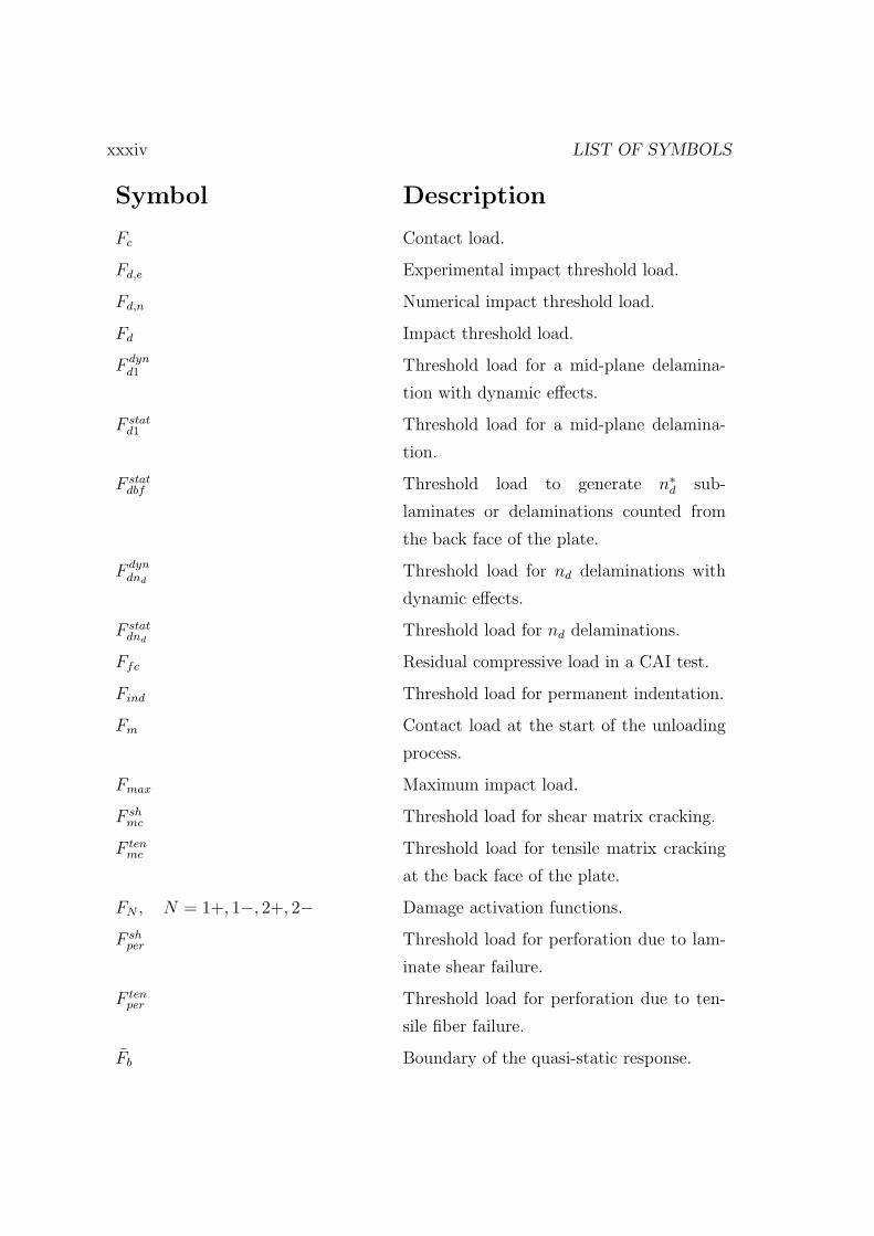
Symbol Description
Fc Contact load.
Fd,e Experimental impact threshold load.
Fd,n Numerical impact threshold load.
Fd Impact threshold load.
F dynd1 Threshold load for a mid-plane delamina-
tion with dynamic effects.
F statd1 Threshold load for a mid-plane delamina-
tion.
F statdbf Threshold load to generate n∗d sub-
laminates or delaminations counted from
the back face of the plate.
F dyndnd
Threshold load for nd delaminations with
dynamic effects.
F statdnd
Threshold load for nd delaminations.
Ffc Residual compressive load in a CAI test.
Find Threshold load for permanent indentation.
Fm Contact load at the start of the unloading
process.
Fmax Maximum impact load.
F shmc Threshold load for shear matrix cracking.
F tenmc Threshold load for tensile matrix cracking
at the back face of the plate.
FN , N = 1+, 1−, 2+, 2− Damage activation functions.
F shper Threshold load for perforation due to lam-
inate shear failure.
F tenper Threshold load for perforation due to ten-
sile fiber failure.
Fb Boundary of the quasi-static response.

xxxv
Symbol Description
Fhs,max Maximum normalized impact force for half-
space behavior.
Fhs Normalized impact force for half-space be-
havior.
Fmax Maximum normalized impact force.
Fq,max Maximum normalized impact force for
quasi-static behavior.
Fq Normalized impact force for quasi-static be-
havior.
Fw,max Maximum normalized impact force for infi-
nite plate behavior.
Fw Normalized impact force for infinite plate
behavior.
g Acceleration due to the gravity.
g Pure mode fracture toughness ratio.
gM , M = 1+, 1−, 2+, 2−, 6 Dissipated energy by unit of volume at
an integration point (intralaminar damage
model).
ge Dissipated energy by unit of volume at
an integration point (interlaminar damage
model).
G Complementary free energy density.
G Isotropic shear elastic modulus.
G (∆) Monotonic loading function.
Gij, i, j = 1, 2, 3 or i, j = r, θ, z Shear elastic modulus.
Gm Interface shear elastic modulus.
Go (β) Delamination onset criterion defined by
elastic terms.

xxxvi LIST OF SYMBOLS
Symbol Description
GE1+ Fracture toughness in the exponential soft-
ening branch for longitudinal tensile.
GL1+ Fracture toughness in the linear softening
branch for longitudinal tensile.
GI Energy release rate in mode I.
GIc Fracture toughness in pure mode I.
GII Energy release rate in mode II.
GIIc Fracture toughness in pure mode II.
GM , M = 1+, 1−, 2+, 2−, 6 Fracture toughnesses.
Gshearc Fracture toughness in pure mode II.
Gshear Shear energy release rate.
GT Total energy release rate.
Gc Critical energy release rate.
h Plate thickness.
ha Laminate thickness.
hc Thickness of the central cut laminate (TCT
tests).
he FE thickness.
(he)max Maximum finite element thickness.
hp Clustering thickness (ply thickness).
hpp Thickness of a single pre-preg ply.
H Lamina compliance tensor for intralaminar
damage model.
H0 Undamaged compliance tensor.
I1 Mass by in-plane surface unit.
I2 Mass by length unit.
I3 Rotatory inertia term.
kα Contact stiffness.
xxxvii
Symbol Description
k∗α Linearized contact stiffness.
kΣ Lumped stiffness of the plate and of the
contact law.
kb Bending stiffness of the plate.
kbsm Lumped shearing, bending and membrane
stiffness of the plate.
ki, i = x, y Wave numbers.
km Membrane stiffness of the plate.
k∗m Linearized membrane stiffness of the plate.
ks Shearing stiffness of the plate.
ky Linearized contact stiffness with plasticity.
kH Hertz contact stiffness.
K Kinetic energy.
K Penalty stiffness of an interface.
K1 Penalty stiffness of an interface in pure
mode I.
K2 Penalty stiffness of an interface in pure
shear mode.
Kij Dimensionless shear correction factors.
lcz Length of the cohesive zone.
le In-plane element size.
`∗ Characteristic finite element length.
`∗max Maximum characteristic element length.
`min Minimum dimension of an element.
`x Finite element length at x direction.
`y Finite element length at y direction.
L Half specimen length (MMB or ENF tests).
L Lagrangian function.

xxxviii LIST OF SYMBOLS
Symbol Description
L Length of a TCT specimen.
Mi Impactor mass.
Mj, j = 1, 2 Bending moments respect x (i = 1) and y
(i = 2) axis.
ML Mismatch bending stiffness parameter for
two-layer plates.
MM Mismatch bending stiffness parameter.
Mp,max Largest plate mass which can remain unaf-
fected by the boundaries.
Mp,wave Mass of the plate area affected by the first
wave.
Mp Lumped mass of the structure.
M∗p Equivalent lumped mass of the structure.
Mx,My,Mxy In-plane laminate moments.
n Number of same thickness plate regions.
nj, j = 1, 2, 3 Unitary normal vector to a delamination
plane.
nd Number of interfaces for delamination.
n∗d Number of delaminations.
Ne Number of elements in a cohesive zone.
Nx, Ny, Nxy In-plane laminate forces.
N (uo, vo, wo) Non-linear terms of the plate governing
equations.
p(r) Normal contact pressure of the Hertz con-
tact theory.
p0 Maximum normal contact pressure.
P Normal contact pressure.
PB Percent of bending in CAI test.

xxxix
Symbol Description
Pc Critical load for crack propagation (MMB,
ENF and TCT tests).
q Power parameter of the contact law.
q(x, y, t) Concentrated impact force.
Qα Effective contact modulus.
Qx, Qy Through-the-thickness shear forces.
Qzi Effective contact modulus along the loading
axis z of the impactor.
Qzp Effective contact modulus along the loading
axis z of the plate.
rc Radial position of an arbitrary point in the
contact zone.
rn(θ) Position of the leading edge of the n-th wave
mode.
rN , N = 1+, 1−, 2+, 2− Elastic domain thresholds.
rp Plate radius.
R Impactor tip radius.
Rc Contact radius of the Hertz contact theory.
s Unloading rigidity.
SL Longitudinal shear strength of a ply.
SisL In-situ longitudinal shear strength of a ply.
ST Transverse shear strength (transverse com-
pressive fracture).
Su Fiber shear strength.
t Time.
ti Impact time.
ths Normalized impact time at the maximum
impact force for half-space behavior.

xl LIST OF SYMBOLS
Symbol Description
tq Normalized impact time at the maximum
impact force for quasi-static behavior.
tw Normalized impact time at the maximum
impact force for finite plate behavior.
T Surface tractions per unit area.
ufc Compressive displacement at failure.
U Elastic energy or internal work.
vL Loading velocity.
V External work.
V (t) Impactor velocity.
V0 Initial impactor velocity.
Vind Impact velocity for permanent indentation.
V comper Impact velocity for perforation due to lam-
inate compressive failure.
V shper Impact velocity for perforation due to lam-
inate shear failure.
wb Displacement of the back face of the plate
at the impact point.
wi Displacement of the impactor.
wo Displacement of the mid-plane of the plate
at the impact point.
W Total length of a TCT specimen.
W Total work.
WC Work done by contact penalties.
WE External work.
WI Internal work.
Wmn(t), Xmn(t) and Ymn(t) Coefficients of Fourier series (complete an-
alytical impact models).

xli
Symbol Description
WMS Work done in propelling mass added in
mass scaling.
XPO Pull-out strength.
XC Longitudinal (fiber) compression strength.
XT Longitudinal (fiber) tensile strength.
Y Thermodynamic force.
YC Transverse compressive strength of a ply.
YT Transverse tensile strength.
Y isT In-situ transverse tensile strength.
α Indentation.
α0 Fracture angle.
α0 Permanent indentation.
αcr Critical indentation as from of it permanent
indentation starts.
αii, i = 1, 2 Coefficients of thermal expansion.
αmax Maximum indentation.
β Characteristic impact parameter.
β Mixed-mode ratio.
βii, i = 1, 2 Coefficients of hygroscopic expansion.
γij, i, j = x, y, z or i, j = 1, 2, 3 Shear strains.
δt Increment of time.
δtstable Stable time increment (FE explicit algo-
rithm).
δ Variational operator.
δ(·) Dirac delta function.
δij, i, j = 1, 2, 3 Kronecker delta operator.
xlii LIST OF SYMBOLS
Symbol Description
δLP Displacement at LP point (MMB tests).
δM Displacement at M point (MMB and ENF
tests).
∆M Difference of moisture content respect to
the corresponding reference value.
∆T Difference of temperature respect to the
corresponding reference value.
∆f Propagation criterion for delamination.
∆o Onset criterion for delamination.
∆shear Euclidian norm of the relative displace-
ments in mode II and mode III.
∆fshear Relative displacement for damage propaga-
tion in shear mode.
∆oshear Relative displacement for damage onset in
shear mode.
∆f3 Relative displacement for damage propaga-
tion in pure mode I.
∆o3 Relative displacement for damage onset in
pure mode I.
∆i, i = 1, 2, 3 Relative displacements.
∆ Relative displacement vector.
εoi , i = q, r Transverse shear strains.
εoi , i = x, y, s In-plane stretching and shearing of the mid-
plane (membrane strains).
εi, i = x, y, z, q, r, s or i = 1, . . . , 6 Contracted notation of the strain.
εij, i, j = x, y, z or i, j = 1, 2, 3 Tensorial strain notation.
εSG1 Strain lecture from a gage located on the
top face of a plate (CAI test).

xliii
Symbol Description
εSG3 Strain lecture from a gage located on the
bottom face of a plate (CAI test).
εc Through-the-thickness compressive failure
strain.
ζ, (or ζw = ζ/2) Relative plate mobility, inelastic parameter,
or loss factor.
η Least-square fitting parameter of interlam-
inar fracture toughnesses.
ηL Longitudinal friction coefficient.
ηT Coefficient of transverse influence (trans-
verse compressive fracture).
θ Off-axis loading axis or orientation of a ply.
θs Sliding angle (transverse compressive frac-
ture).
κi, i = x, y, s Curvatures.
λ Norm of the relative displacement compo-
nents.
λ Relative stiffness.
λi, i = x, y Wavelengths.
µ Effective mass ratio.
µ Friction coefficient.
ν Isotropic Poisson ratio.
νij, i, j = 1, 2, 3 or i, j = r, θ, z Poisson coefficients.
νm Interface Poisson ratio.
Ξ Computed energy dissipated by delamina-
tion.
Π Total potential energy.
ρ Density.

xliv LIST OF SYMBOLS
Symbol Description
ρm Density of the interface material.
σfc Residual compressive strength in a CAI
test.
σi, i = x, y, z, q, r, s or i = 1, . . . , 6 Contracted notation of the stress.
σij, i, j = x, y, z or i, j = 1, 2, 3 Tensorial stress notation.
σyc Compressive elastic limit of the plate in the
through-the-thickness direction.
(σ1, σ2, σ6)p Stress components on the back outer ply of
the laminate.
(σx)max and (σy)max Maximum values of the in-plane tensile
stresses due to the flexural deformation.
σ(m) Components of the stress tensor defined in
a coordinate system (m) representing the
fiber misalignment.
σ Effective stress tensor.
τ Mixed-mode interface stress.
τ o Mixed-mode interface strength.
τ o1 Shear pure mode interface strength.
τ o3 Pure mode I interface strength.
τij, i, j = x, y, z or i, j = 1, 2, 3 Shear stresses.
τmax Maximum allowable frictional shear stress.
τi, i = 1, 2, 3 Interface stresses.
τTeff and τLeff Effective stresses (transverse compressive
fracture).
φi, i = 1, 2 Rotations of a transverse normal about the
y (i = 1) and x (i = 2) axis.
φN , N = 1+, 1−, 2+, 2− Loading functions.
ϕC Fiber misalignment angle.
xlv
Symbol Description
Ψ Helmholtz free energy.
Ψo (β) Elastic energy of the interlaminar constitu-
tive equation.
Ψo Function of the relative displacement space.
ωmn Natural frequencies of a plate.
(r, θ, z) Cylindrical coordinates of the plate.
(u, v, w) Displacements of the plate at (x, y, z).
(u1, u2, u3) Displacements of the plate at (x1, x2, x3).
(uo, vo, wo) Mid-plane displacements of the plate at
(x, y, z).
(x, y, z) Cartesian coordinates of the plate.
(x1, x2, x3) Cartesian coordinates of the ply.
[C]p Constitutive matrix of the back outer ply
in the ply coordinate system.
[S] Compliance matrix of the plate in the plate
coordinate system.
[T ]γ Rotation matrix of the engineering strains
from the plate coordinate system to the ply
coordinate system.

xlvi LIST OF SYMBOLS

List of Acronyms
Acronym Description
AFP Automated Fiber Placement.
AITM AIrbus Test Method.
ASTM American Society for Testing Materials.
BVID Barely Visible Impact Damage.
CAI Compression After Impact.
CFRP Carbon Fiber Reinforced Plastic.
CMC Ceramic Matrix Composite.
CPU Central Processing Unit.
DIC Digital Image Correlation.
ENF End-Notched Flexure test.
FE Finite Element.
GB Giga-Byte.
GFRP Glass Fiber Reinforced Plastic.
GLARE GLAss REinforced fiber metal laminate.
LaRC Langley Research Center (failure criteria).
LEFM Linear Elastic Fracture Mechanics.
LVDT Linear Variable Differential Transformer.
MMB Mixed-Mode Bending test.
MMC Metal Matrix Composite.
MPI Message Passing Interface mode.
xlvii

xlviii LIST OF ACRONYMS
Acronym Description
NDI Non-Destructive Inspection methods.
PMC Polymeric Matrix Composite.
RAM Random-Access Memory.
SG Strain Gage.
TCT Transverse Crack Tension test.
UEL User ELement subroutine (Abaqus/Implicit code).
VCCT Virtual Crack Closure Technique.
VUEL User ELement subroutine (Abaqus/Explicit code).
VUINTER User INTERaction subroutine (Abaqus/Explicit code).
VUMAT User MATerial subroutine (Abaqus/Explicit code).

Chapter 1
Introduction and objectives
1.1 Introduction
A composite material is defined as the combination of two or more phases on the
macroscopic scale. The mechanical performance and properties of the composite are
superior to those of the individual constituent materials.
Typically, composite materials are classified in function of the reinforcement
geometry, or in function of the matrix material. Related to the geometry of the
reinforcement, it can be composed by long fibers, short fibers, or particles. The
fibers can be presented randomly distributed, following an established direction in
the composite, or even as a fabric. Related to the matrix material, the most typical
are Polymeric Matrix Composite (PMC), Metal Matrix Composite (MMC), and
Ceramic Matrix Composite (CMC).
When the PMC is reinforced by long fibers, it is called advanced Fiber Reinforced
Plastic (FRP), using for example glass (GFRP) or carbon (CFRP). Advanced FRPs
are often fabricated in the form of laminates. A laminate consists of one or more
thin layers (laminae or ply) stacked together, where each one has the reinforcement
oriented at one given direction, in the form of unidirectional plies. The orientation
of each ply is changed suitably in order to stand the mechanical design requests.
Nowadays, there are manufacturing systems completely automatized, Automated
Fiber Placement machine (AFP), that stack each ply according to the final geometry
of the structure and with the desired fiber orientation, or even with orientations that
change point to point (curved fibers).
1

2 CHAPTER 1. INTRODUCTION AND OBJECTIVES
The application of advanced FRPs is gradually increasing as a result of their
good specific mechanical properties and increased flexibility of design. Compos-
ites are used in a wide spectrum of industrial components and customers, where
the aerospace industry, including military and commercial aircraft, is the largest
consumer [1].
At present, the advanced FRPs are included in the set of materials that improve
and advance the aviation industry. In this field, it is well known that the main
issues of concern are the greenhouse gas emissions and the fuel costs, which are the
largest operating expense for airlines. The development of technologies to address
these issues has clear economic and environmental benefits. As documented by King
et al. [2], the reduction of the amount of fuel burnt can be achieved by ”reducing
both aircraft weight and its parasitic drag (drag due to the non-lift component, i.e.
the fuselage)”. In this sense, the application of advanced FRPs in primary and
secondary structures is taking part in the improvement of the whole weight due to
the good combination of light weight, and high stiffness and strength.
When composites are to be used in structural components, a design development
program is generally initiated during which the performance of the structure is
assessed prior to its use. Typically, the process of design starts with the analysis of
a large set of simple small specimens and, when sufficient knowledge is acquired at
this level, it is changed over to a more complex structure but carrying out fewer tests.
This process is repeated until to reach the complete full scale product, at which one
or two very expensive tests are performed. This process is commonly known as
the Building Block approach [3]. At each step of this approach, a combination of
testing and analysis techniques is typically performed, because testing alone can be
prohibitively expensive due to the large number of specimens needed to verify every
geometry, loading, environment, and failure mode [4].
As reported Davies and Ankersen [5], design time is expensive and structural
testing is also expensive, of the order of $40 million for a new aircraft variant.
Therefore, the development of reliable analysis tools that enable to understand the
structure mechanical behavior, as well as to replace most, but not all, the real
experimental tests, is clear interest. Recent advances in simulation by means of
computers, known as Virtual Mechanical Testing, have given realistic models for
the prediction of the complicated physical processes involved in the behavior of

1.1. INTRODUCTION 3
composite materials. These models are of special interest in configurations that are
too complex to certify by purely empirical methods.
During all the stages of the certification process for aeronautic structures, two
key concepts are permanently addressed: damage resistance (or durability), and
damage tolerance. As reported by Bailie et al. [6], ”the damage resistance is the
ability of the structure to resist damage initiation and/or growth for a specified length
of time. How durable the structure should be designed to be is an economic issue. A
highly durable structure requires fewer inspections and repairs”. On the other hand,
”the damage tolerance is the ability of the structure to resist catastrophic failure
in the presence of cracks or other damage without being repaired, for a specified
number of operations (flights) or length of time in service. Damage tolerance is
usually demonstrated by residual strength tests conducted on a component that has
been previously damaged in a well defined manner. Residual strength must be greater
than a limit value, defined by the certifying authority, that depends on the ability to
detect the damage during an inspection”.
It is well known that laminated composite structures have excellent fatigue lives
compared to metallic structures. However, they are specially weak to environment
changes and impact loadings.
An impact is a dynamic event where the contact of the collided bodies generates
forces that act in a very short interval of time, and initiate stress waves which
travel away from the region of contact. Impacts by foreign objects can be expected
during all the stages of the life of the composite structure (manufacturing, service
and maintenance). The design of impact damage resistant and damage tolerant
composite components is a conceptually difficult task. Unlike metallic components,
which can yield and dissipate energy via plasticity, composites dissipate energy by a
variety of interacting damage modes. The damage created often cannot be detected
by simple visual inspection, can grow under load, and can cause severe reductions in
the stiffness and the strength. Lack of knowledge of the impact effects on composite
structures is a factor in limiting the use of composite materials [7].

4 CHAPTER 1. INTRODUCTION AND OBJECTIVES
1.2 Motivation
Susceptibility to damage from concentrated out-of-plane impact forces is one of the
major design concerns of structures made of advanced FRPs used in the aeronauti-
cal industry. The development of virtual mechanical testing models to analyze the
impact damage resistance of a structure is of great interest for reducing certifica-
tion costs. But even more, the prediction of the residual strength of the impacted
structure is the most valuable data. However, it is a difficult task.
When an impact is given on a composite structure, the description of the problem
is quite complex. Laminated composites are heterogeneous materials due to presence
of local flaws, such as air micro-gaps, resin-rich zones, discontinuities of the fibers,
loss of fiber lineup, changes of fiber density, etc. Accordingly, composite structures
degrade in a large variety of failure mechanisms (matrix cracking, fiber-matrix inter-
face debonding, delamination, and fiber breakage) which interact in a complicated
way, especially when the structure is subjected to impact loading. Moreover, the
onset and the evolution of these failure mechanisms depend on a large set of impact
parameters, that are the physical parameters and properties of the projectile, the
structural configuration, and the environmental conditions. Due to all these facts,
the development of a reliable tool for the prediction of the impact damage resistance
and the corresponding damage tolerance is a challenging task, which at present, it
is not available.
Analytical impact models representing the physical system must be considerably
idealized to render them amenable for a possible theoretical treatment. Conse-
quently, the solutions obtained often are valid for a narrow range of impact config-
urations, or even they are not suitable because the predictions are too far from the
reality.
Using the major recent advances in computational methods and the conceptual
representation of the composite failure mechanisms, the virtual testing of the impact
event by means of numerical simulations of finite element (FE) codes seems to
be reachable. The proposal of modeling impact in a FE code is in part possible
due to the advances in Computer Sciences which allow enough detailed description
of the event with acceptable analysis runtime. This is succeed by means of the
parallelization of the FE model in multiple CPUs, i.e. using a cluster.

1.3. OBJECTIVES 5
In contrast to the analytical models, FE methods are capable of modeling large
number of impact configurations and several related phenomena, such as dynamic
modeling, contact analysis, and progressive degradation of the material. The ma-
terial behavior can be described by the implementation of constitutive models for-
mulated in the framework of Continuum Damage Mechanics. One of the main keys
for the realistic prediction of the virtual testing is the suitable formulation of the
constitutive models.
1.3 Objectives
The main goal of the present thesis is the development of a FE tool for the simulation
of two sequenced and standardized tests, drop-weight impact and Compression After
Impact (CAI), on specimen coupons manufactured with polymer-based composite
materials reinforced with continuum fibers. Drop-weight impact is categorized as
a low-velocity and large mass impact test. Under this loading, the delamination is
the major damage mechanism as it reduces considerably the compressive strength
of the structure. On that account, the CAI test is performed to assess the effect
of the impact damage on the compressive strength. Therefore, the purpose of the
simulations is the prediction of the residual compressive strength of the correspond-
ing impacted specimen; to achieve this goal, the previous simulation of the impact
should be accurately performed.
The reliability of the predictions depends mainly on the constitutive model for
the description of the composite material behavior. That is the description of the
onset and the growth of the different damage mechanisms. The strategy used here
is based on modeling the laminate failure, where a laminate consists of homoge-
neous plies, each with orthotropic properties that depend on the fiber orientation.
Accordingly, two separated constitutive models are formulated using a rigorous ther-
modynamic framework: one for the description of the debonding between the plies
of the laminate (i.e. delamination), and another for the description of the dam-
age mechanisms that can occur in each ply (i.e. intralaminar damage mechanisms:
matrix cracking, fiber-matrix interface debonding, and fiber breakage). The formu-
lation and implementation of both constitutive models are performed separately,
but the interaction of the damage mechanisms is ensured since both damage models
6 CHAPTER 1. INTRODUCTION AND OBJECTIVES
are used in the same FE model. The proposed delamination model and intralaminar
model are respectively based on previous thesis and papers presented by Turon et
al. [8–13] and Maimı et al. [14–17].
Other aims of the present project, that are as relevant as the FE predictions, are
the analytical description of the impact event and the realization of an experimental
test plan. The FE simulations need an appropriate experimental program to assess
the validity of the numerical predictions.
Also, due to the simplicity of the structure considered (monolithic, flat and
rectangular laminated composite plates with conventional stacking sequences), the
analytical description of the impact event is feasible. This analytical description
comprises the prediction of the elastic response and the proposals of new thresh-
olds at which significant damage starts. The analytical description is suitable for
preliminary design analysis, as it enables the fast assessment of the role that each
parameter plays in the impact event. Accordingly, the analytical description is use-
ful for the definition of impact experimental plans. Although the analytical tools
studied herein are focused on laboratory coupons, the concepts acquired often can
be applied for more complex impact configurations.
Since the experimental drop-weight impact and CAI tests are performed with
the goal of having real data to validate the results obtained by means of the FE
simulations, the impact configurations considered should assure the damage occur-
rence. Because of that, the design of the experimental plan is carried out by means
of the analytical impact models.
1.4 Thesis lay-out
According to the objectives described previously, the thesis is structured as follows:
In Chapter 2 and in the related Appendix A, a detailed review of the analyti-
cal impact models available in the bibliography is given. This review includes the
models for the prediction of the elastic impact response, as well as the description of
available and new proposals for damage thresholds. By means of this analysis, the
experimental plan and set-ups of the drop-weight impact and CAI tests are defined
in Chapter 3.
In Chapter 4, the significant experimental results of the drop-weight impact

1.4. THESIS LAY-OUT 7
tests, the non-destructive inspections, and the CAI tests are shown and discussed.
Additionally, comparisons with analytical predictions are also carried out.
Related to the development of FE simulations, an interlaminar damage model
for the simulation of the delamination onset and growth under variable mixed-mode
conditions is developed in Chapter 5. The formulation and implementation pre-
sented is a modified proposal of the model originally developed by Turon et al.
[8–13]. The model is validated by simulating quasi-static standard delamination
toughness tests and by comparing the results with experimental data.
In Chapter 6, the formulation of a continuum damage model for the prediction
of the onset and accumulation of intralaminar damage mechanisms in laminated
composites is described. The model presented is based on the work developed by
Maimı et al. [14–17]. In this chapter, simulations of different tests in order to
illustrate the limitations of using a constitutive damage model formulated in the
Continuum Damage Mechanics framework are presented.
Using the damage models developed, some of the impact and CAI tests which
are tested experimentally are also simulated. The considerations for the proper
simulation of the tests are detailed in Chapter 7, as well as the virtual results and
their comparison with the experimental data presented previously in Chapter 4.
Finally, the thesis is concluded in Chapter 8 with an overall assessment of its
achievements and a discussion of possible future research developments.

8 CHAPTER 1. INTRODUCTION AND OBJECTIVES

Chapter 2
Analytical description of the
impact event
2.1 Introduction
The prediction of damage in laminated composite structures induced by the impact
of an external object is a complex task. Damage results from the interaction between
different failure mechanisms (matrix cracking, fiber-matrix interface debonding, de-
lamination, and fiber breakage), and it depends on the governing parameters of the
impact event. These parameters include the physical parameters and properties of
the projectile, the structural configuration, and the environmental conditions.
Experimental evidence shows that impact damage is directly related to the na-
ture of the impact behavior which, in turn, is controlled by the governing param-
eters. Therefore, it is useful to know the effects of each governing parameter on
the impact behavior, and thus to have a qualitative understanding of the possible
damage mechanisms that can occur. For example, under constant energy impact
conditions, a quasi-static type of impact behavior will result mostly in delamina-
tion damage whereas in a dilatational wave-controlled type of impact behavior will
result mostly in permanent indentation and fiber breakage at the impact site [18].
There are approaches in the literature, based on analytical models, which predict
the type of the impact response for a determined configuration, such as impact on
flat and rectangular laminated composite plates [19, 20]. The initial knowledge of
the impact behavior not only helps in assessing the possible type of damage induced,
9

10 CHAPTER 2. ANALYTICAL DESCRIPTION OF THE IMPACT EVENT
but it is also useful for the development of efficient numerical models, for planning
test programs, and for selecting a proper simplified analytical model to describe the
impact event.
The analytical models are a suitable and powerful tool to obtain fast predictive
results for a given impact configuration. Generally, these analytical models are lim-
ited to simple geometries of the structure and rely on stepwise solution of nonlinear
differential equations or integral equations which describe the transitory response
of the system until damage onset, i.e. in the elastic regime. The results given by
these analytical models are suitable to compare different impact cases with different
values of the governing parameters.
The framework and the ingredients used for the impact dynamics description on
rectangular, flat, and monolithic laminated composite plates are presented in this
chapter. Therefore, a literature survey of the analytical impact models available
is presented. On the other hand, an overview of the main approaches used to
identify quickly the nature of the impact behavior is done. Finally, a review of the
analytical damage thresholds available in the literature, as well as the development
of new proposals for some damage mechanisms are presented.
The issues analyzed in this chapter and in the related Appendix A are used to
define a suitable set of low-velocity impact tests in order to capture different damage
phenomena which can occur. The details of this task are described in Chapter 3.
2.2 Impact behavior
Experimental evidence shows that the nature of the impact behavior and the re-
sulting damage are related. Since the impact behavior is defined by the governing
parameters of the impact event, the damage created also depends on these pa-
rameters. For impacts on rectangular, flat, and monolithic laminated composite
plates, the governing parameters are typically grouped in three sets: plate param-
eters (thickness, in-plane size, lamina type, elastic and fracture properties, density,
stacking sequence, and boundary conditions), impactor parameters (shape, size,
elastic properties, mass, velocity, and incidence angle), and the environmental con-
ditions.
The impact behavior can be predicted easily in the elastic regime by means of

2.2. IMPACT BEHAVIOR 11
approaches based on analytical models of the impact event. Thus, the information
obtained can be used to know the possible related damage which can occur. Damage
starts when a suitable parameter of the elastic response, typically the impact force,
is greater than the corresponding damage threshold (see Section 2.6).
Before to describe the models for the prediction of the impact response, it is useful
to review the different types of impact responses for plates (impact behaviors), as
the response type is crucial to have a qualitative insight of the resulting possible
damage, and for the selection of a simplified model for impact description. Detailed
descriptions of the impact behaviors are given by Olsson [20–25], by Christoforou
and Yigit [18, 19, 26, 27], by Abrate [7, 28], and by Lin and Fatt [29].
According to Olsson [22], an impact event initiates stress waves propagating
from the impact point, where the influence of the waves gradually fade away due
to material damping and wave scattering. For impact times ti close to the time
required for the waves to propagate through-the-thickness direction (i.e. ti ≤ hcz
,
where h is the plate thickness, and cz the speed of sound in the through-the-thickness
direction), the response is dominated by three-dimensional wave propagation (see
Figure 2.1.a). For longer impact times, flexural and shear waves govern the response
(see Figure 2.1.b). For times much longer than the time needed by these waves to
reach the plate boundaries, the lowest vibration mode of the impactor-plate system
predominates (see Figure 2.1.c). Eventually, the deformation mode approaches a
purely static deformation.
The response dominated by through-the-thickness waves is typically associated
with ballistic impact, which in most cases, causes localized and easily detectable
damage. Related to the impacts that can have an aircraft, the response in Figure
2.1.b is typical for impacts by hail and runway debris, whereas the response in Figure
2.1.c is typical for dropping of heavy tools. The in-plane plate size and the boundary
conditions affect the response shown in Figure 2.1.c, but not the responses shown in
Figures 2.1.a and 2.1.b, because in these cases, the impact event is over before the
stress waves have reached the edges of the structure. The load and the deflection are
out of phase during a small mass impact while they are more or less in phase during
a large mass impact. Furthermore, due to the more localized deflection, small mass
impactors cause higher impact loads and earlier damage initiation than large mass
impactors with the same kinetic energy.

12 CHAPTER 2. ANALYTICAL DESCRIPTION OF THE IMPACT EVENT
(a) (b) (c)
Figure 2.1: Impact responses (after Olsson [22]): (a) dominated by dilatational
waves, (b) dominated by flexural and shear waves, and (c) quasi-static response.
Summarizing, the impact behaviors can be classified into three extreme cate-
gories that are referenced in the literature as: (a) three-dimensional wave-controlled,
through-the-thickness wave-controlled or ballistic impact ; (b) global behavior with no
size effects, flexural and shear wave-controlled, or impact on an infinite plate; (c)
fully-global or quasi-static impact behavior. If the global response of the plate can
be neglected (extreme case of (b)), this impact behavior is typically called half-space
impact.
Clear Visible Impact Damage is associated with the response shown in Figure
2.1.a. In addition, Barely Visible Impact Damage (BVID) is associated with the
response types shown in Figures 2.1.b and 2.1.c [6], where delamination is the main
damage mechanism. Delaminations are a major threat because they are hidden and
reduce significantly the compressive strength of the impacted structure.
Impacts are often categorized in the literature as low- or high-velocity, but there
is not a clear transition between categories and authors disagree on its definition
[30]. Some authors refer, improperly, to the response type under small mass of
the impactor as high-velocity impact and under large mass impact as low-velocity
impact. Olsson [20], and Christoforou and Yigit [19] demonstrate that the response
type under elastic conditions depends on the impactor mass, the mass of the surface
of the plate affected by the impact and the structural stiffness. Increasing the
velocity, the impact force increases and induces a large damage extension or even
a change in the main damage mechanism type, but the velocity does not affect the
impact behavior. The classification by means of the velocity may be motivated
from a practical point of view for damage creation, since large mass impactors

2.3. LOCAL DEFLECTION 13
usually cause damage at a lower velocity than small mass impactors with the same
kinetic energy. When an impact is categorized as low-velocity impact, the material
properties are assumed to be rate independent [31].
A physically based criterion to distinguish low- or high-velocity impact categories
was suggested in Davies and Godwin [32], which defined high-velocity impact as
cases where the ratio of the impactor velocity V0 versus the speed of sound in the
plate thickness direction cz, exceeds the through-the-thickness compressive failure
strain εc. That is:
εc =V0
cz(2.1)
The assumed failure mode implies a response governed by through-the-thickness
waves (i.e. ballistic impact). For typical composite materials, the corresponding
impactor velocity ranges from 10 to 20m/s [33]. However, the large strains associated
with contact stresses are highly localized and the resulting failure may often not
affect the general response of the plate. Thus, response governed by flexural and
shear waves has been experimentally demonstrated in carbon/epoxy laminates at
velocities of 45m/s. Thus, the use of velocity for classifying impact events is highly
debatable [20].
Finally it should be noted that the term hyper-velocity has come to be applied to
satellites and spacecraft which may be struck by micro-meteorites where the impact
duration is measured in nanoseconds, and both the meteorite and impacted structure
will vaporize [21].
2.3 Local deflection
Impact on monolithic plates involves local and global deflection. Therefore, impact
damage may be caused due to local contact stresses and/or stresses resulting from
the structural response. Figure 2.2 shows two extreme responses of a plate under
impact loading. Only local deflection is shown in Figure 2.2.a, which can result from
small-mass and high-velocity impact on thick laminate plates. However, only global
deflection is shown in Figure 2.2.b, which can occur from large-mass and low-velocity
impact on thin laminate plates.
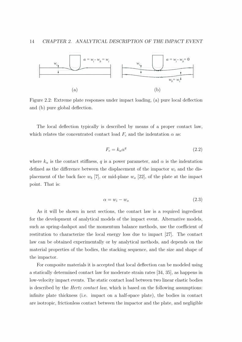
14 CHAPTER 2. ANALYTICAL DESCRIPTION OF THE IMPACT EVENT
(a) (b)
Figure 2.2: Extreme plate responses under impact loading, (a) pure local deflection
and (b) pure global deflection.
The local deflection typically is described by means of a proper contact law,
which relates the concentrated contact load Fc and the indentation α as:
Fc = kααq (2.2)
where kα is the contact stiffness, q is a power parameter, and α is the indentation
defined as the difference between the displacement of the impactor wi and the dis-
placement of the back face wb [7], or mid-plane wo [22], of the plate at the impact
point. That is:
α = wi − wo (2.3)
As it will be shown in next sections, the contact law is a required ingredient
for the development of analytical models of the impact event. Alternative models,
such as spring-dashpot and the momentum balance methods, use the coefficient of
restitution to characterize the local energy loss due to impact [27]. The contact
law can be obtained experimentally or by analytical methods, and depends on the
material properties of the bodies, the stacking sequence, and the size and shape of
the impactor.
For composite materials it is accepted that local deflection can be modeled using
a statically determined contact law for moderate strain rates [34, 35], as happens in
low-velocity impact events. The static contact load between two linear elastic bodies
is described by the Hertz contact law, which is based on the following assumptions:
infinite plate thickness (i.e. impact on a half-space plate), the bodies in contact
are isotropic, frictionless contact between the impactor and the plate, and negligible

2.3. LOCAL DEFLECTION 15
curvature of the plate surface during contact (i.e. the wrapping effect is neglected).
The Hertz contact law has been applied in a wide range of cases even when if
all assumptions are not satisfied (e.g. indentation on laminated composite plates),
because usually it fits quite well the experimental data obtained from indentation
tests.
In the literature there are advanced developments for the contact description
which take into account the anisotropy of laminated composite materials. These
models are not often simple as the Hertz contact law, because the resulting laws
require the numerical solution of differential or integral equations. Some examples
for transversely isotropic materials are the work presented by Dahan and Zarka [36],
and Turner [37]. For orthotropic materials, the work of Wu and Yen [38], Chao and
Tu [39], and Swanson [40] should be mentioned.
A comprehensive justification of the Hertz contact law agreement for local de-
flection modeling of laminated composite plates in contact with a hemispherical
indentor, and a collection of some developments available in the literature to get
over some of the Hertz assumptions are given by Abrate [7], and Davies and Olsson
[21]. In [21], the descriptions are given in function of the static indentation tests
which can be performed:
• Measuring differences between front and back face deflections on
plates with an unsupported back face. This test is suitable for lo-
cal deflection analysis in flexible plates. Under low contact loads, the load-
indentation behavior is in agreement with the Hertz contact law [41, 42]. Under
high contact loads, the plate may result in a large flexural curvature, which
increases the contact area (i.e. the wrapping effect). Also, matrix cracking and
delamination reduces the flexural stiffness which contributes to a large flexural
curvature. Due to this increase of the contact area, the pressure distribution
changes from a bell-shaped (Hertzian-type distribution) to a saddle-shaped.
As a result of this redistribution, the indentation decreases as the force keeps
increasing [7]. However, this effect has a small influence on the response, which
is then dominated by global plate deflections.
• Placing the plate on a flat rigid support. This test is suitable for the
local deflection analysis in rigid plates. Under low contact loads, the load-
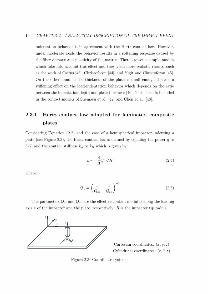
16 CHAPTER 2. ANALYTICAL DESCRIPTION OF THE IMPACT EVENT
indentation behavior is in agreement with the Hertz contact law. However,
under moderate loads the behavior results in a softening response caused by
the fiber damage and plasticity of the matrix. There are some simple models
which take into account this effect and they yield more realistic results, such
as the work of Cairns [43], Christoforou [44], and Yigit and Christoforou [45].
On the other hand, if the thickness of the plate is small enough there is a
stiffening effect on the load-indentation behavior which depends on the ratio
between the indentation depth and plate thickness [46]. This effect is included
in the contact models of Suemasu et al. [47] and Chen et al. [48].
2.3.1 Hertz contact law adapted for laminated composite
plates
Considering Equation (2.2) and the case of a hemispherical impactor indenting a
plate (see Figure 2.3), the Hertz contact law is defined by equaling the power q to
3/2, and the contact stiffness kα to kH which is given by:
kH =4
3Qα
√R (2.4)
where:
Qα =
(1
Qzi
+1
Qzp
)−1
(2.5)
The parameters Qzi and Qzp are the effective contact modulus along the loading
axis z of the impactor and the plate, respectively. R is the impactor tip radius.
Cartesian coordinates: (x, y, z)
Cylindrical coordinates: (r, θ, z)
Figure 2.3: Coordinate systems.

2.3. LOCAL DEFLECTION 17
The normal contact pressure p(r) of the Hertz theory varies within the contact
radius Rc as:
p(r) = p0
√1− r2
c
R2c
, 0 ≤ rc ≤ Rc (2.6)
Rc =
(3
4
FcR
Qα
) 13
=√Rα (2.7)
where rc is the radial position of an arbitrary point in the contact zone, and p0 is
the maximum pressure located at rc = 0 given by:
p0 =3Fc
2πR2c
(2.8)
For isotropic materials (e.g. a steel impactor), the effective contact modulus is
defined by:
Qz =E
(1− ν2)(2.9)
where E and ν are the Young modulus and the Poisson ratio, respectively. For the
case where the indentor is much stiffer than the plate, Equation (2.5) simplifies to
Qα ≈ Qzp.
The extension of Equation (2.9) for materials with transverse isotropy (along the
loading axis z) is [22]:
Qzp =Ez
(1− νrzνzr)(2.10)
where νrz and νzr are the through-the-thickness Poisson ratios. In most laminate
plates νrzνzr ≈ 0, and Equation (2.10) can be simplified to Qzp = Ez [41, 46]. The
through-the-thickness Young modulus of the laminate Ez is common to set equal to
the transversal Young modulus of a single ply (i.e. Ez = E2).
It is important to remark that Equation (2.10) is an approximation of the ef-
fective modulus of transversally isotropic plates which underestimates the contact
modulus of typical composite plates by 10-20% [23, 40].
More advanced expressions of Qzp for transversally isotropic materials are avail-
able in the literature: Turner [37, 40, 49], or that of Greszczuk [23, 50].
18 CHAPTER 2. ANALYTICAL DESCRIPTION OF THE IMPACT EVENT
The expression of Qzp proposed by Turner [37] is given as:
Qzp =2
β1β3
(2.11)
where:
β1 =
ErEz− ν2
rz
1− ν2rr
1/2
, β2 =
1 +
(Er
2Grz
− 1
)− νrz (1 + νrr)
1− ν2rr
β3 =
(β1 + β2
2
)1/2(1− νrrGrr
)(2.12)
The expression developed by Greszczuk [50] is given as:
Qzp =
2
√Grz
Crr(CrrCzz − C2
rz)
√(√CrrCzz +Gzr
)2 − (Crz +Gzr)2
(2.13)
where:
Crr =Er (1− νrzνzr) Ω
(1 + νrr), Crz = ErνzrΩ
Czz = Ez (1− νrr) Ω, Ω =1
(1− νrr − 2νrzνzr)
(2.14)
In an orthotropic plate, the effective contact modulus Qzp defined by Equation
(2.10) becomes directionally dependent. Then, the shape of the indentation, which
is circular in transverse isotropic plates along z axis, becomes elliptical in orthotropic
plates. The effective contact modulus can be estimated by integrating Er (θ) over
2π and taking the average [22]. However, since in most laminated plates νrzνzr ≈ 0,
the solution again simplifies to Qzp = Ez.
2.3.2 Unloading and reloading contact process
Typically, in an impact event the contact force increases to a maximum value and
then decreases back to zero. During the unloading phase, Yang and Sun [41] found

2.3. LOCAL DEFLECTION 19
that the Hertzian contact law was not adequate. The unloading phase is significantly
different from the loading phase due to permanent indentation. In order to account
this effect, Crook [51] proposed the following equation:
Fc = Fm
(α− α0
αmax − α0
)5/2
(2.15)
where Fm is the contact force at the start of the unloading, αmax is the indenta-
tion corresponding to Fm (i.e. maximum indentation) and α0 is the permanent
indentation. Equation (2.15) can be rewritten as:
Fc = s (α− α0)5/2 (2.16)
where:
s =Fm
(αmax − α0)5/2(2.17)
is called unloading rigidity. Equaling the Hertz contact law for loading with Equation
(2.15), the permanent indentation α0 and the critical indentation αcr as from of it
permanent indentation starts, are given as:
α0 =
αmax
(1−
(αcrαmax
)2/5)
if αmax > αcr
0 if αmax ≤ αcr
(2.18)
αcr =kHs
(2.19)
The procedure in order to define αcr starts by the selection of a proper value of
α0 by means of the unloading contact law (Equation (2.15)), so that the areas under
the analytical unloading curves are equal to that calculated from the corresponding
experimental curves. If these values of α0 are substituted into Equation (2.17), a
range of values of s is obtained. Using the average of s values, the value of αcr is
finally obtained.
If a subsequent reloading phase is done, the contact law is also distinct from the
unloading curve but always returns to the point where unloading began [41]. The
reloading curve is modeled by:

20 CHAPTER 2. ANALYTICAL DESCRIPTION OF THE IMPACT EVENT
Fc = Fm
(α− α0
αmax − α0
)3/2
(2.20)
In this case, there is no need to perform reloading experiments to find the pa-
rameters of the contact law.
2.3.3 Elastic-plastic contact models
Permanent deformations can be introduced in composite materials when the inden-
tation exceeds a critical value because the material behavior is mainly governed
by the properties of the matrix where a plastic behavior is expected. Under this
circumstance, the Hertz contact law overestimates the maximum contact force and
elastic-plastic contact laws can yield more realistic results. In these models, the crit-
ical indentation is taken into account during the loading process, unlike the previous
approach where the critical indentation is accounted for using the unloading phase.
Elastic-plastic models assume that initially the material behaves elastically until
a critical indentation is reached (see Figure 2.4). At this point, the contact area is
divided into a plastic zone and an elastic zone as the loading increases and a new
contact law is obtained [7]. Some elastic-plastic contact models are described below.
The elastic-plastic model developed by Christoforou [44] describes the contact
loading and unloading between a rigid sphere and a thin laminated composite plate
supported on a rigid substrate. Thus, the model is focused only on local deflec-
tions since the global response becomes negligible. The material is assumed to be
transversely isotropic and follows an elastic-perfectly plastic behavior of the through-
the-thickness normal stress-strain law. As yielding stress, a maximum shear failure
criterion governed only by the fiber shear strength Su is considered, although it
is approached to the shear strength of the laminate SL [19]. The development of
Cairns [43] results in the same contact law for loading by assuming that the contact
radius and the indentation are much smaller than the impactor radius.
Therefore, for the loading case, the contact law is defined by:
Fc =
πREz(1− νrzνzr)h
α2 if 0 ≤ α ≤ αcr
2πRSu (2α− αcr) if αcr < α ≤ αmax
(2.21)

2.3. LOCAL DEFLECTION 21
and for the elastic unloading phase, the contact law is:
Fc =πREz
(1− νrzνzr)h(α2 − α2
0
)(2.22)
where h is the specimen thickness. The critical indentation αcr and the permanent
indentation α0 are given by:
αcr =2Suh (1− νrzνzr)
Ez(2.23)
α0 = αmax − αcr (2.24)
Another contact law is proposed by Yigit and Christoforou [45]. It is obtained
by combining the classical Hertz contact theory and the elastic-plastic indentation
theory given in Johnson [34]. In this case, the contact law for loading is given by:
Fc =
kHα
3/2 if 0 ≤ α ≤ αcr
kHα3/2cr + ky (α− αcr) if αcr < α ≤ αmax
(2.25)
and for the elastic unloading phase, the contact law is:
Fc = kH(α3/2 − α3/2
m + α3/2cr
)+ ky (αmax − αcr) (2.26)
where ky is the linear stiffness of the elastic-plastic loading phase which is equal to
the slope of the elastic indentation curve at α = αcr:
ky =3
2kH√αcr (2.27)
The critical indentation αcr can be obtained from the contact stress distribution
using a maximum shear failure criterion [34]. Knowing that YC is the transverse
compressive strength of the laminate, αcr is approached to [26]:
αcr =0.68 (YC)2 π2R
Q2α
(2.28)

22 CHAPTER 2. ANALYTICAL DESCRIPTION OF THE IMPACT EVENT
Figure 2.4: Detail of the contact law phases.
2.3.4 Linearized contact laws
In the analytical models of the impact event (see Section 2.4), the local deflections
are simply described using a proper contact law. When the contact law is replaced
in the governing equations of the plate and of the impactor, an exact solution of
these equations generally are not available and a numerical solution is required.
However, in some cases a closed-form solution can be obtained if the contact law is
linearized (e.g. Christoforou and Swanson [52]; Olsson [35]). The resulting closed-
form equations are more useful to gain a better understanding of the effects of the
governing parameters on the behavior of the impact event.
Yigit and Christoforou [53] proposed a linearization of the elastic-plastic contact
law of Christoforou [44]. Also, the loading contact law presented in [45] is linearized
by Christoforou and Yigit [27], and used in [19, 26, 54]. In addition, Choi and
Lim [55] developed a linearization of the Hertz contact law which allows to model
low-velocity impact problems in a general-purpose finite element method software.
2.4 Analytical impact models
The analytical impact models are a powerful tool to get fast predictive results for
a given impact configuration. These models are usually developed to predict the
response of the system in the elastic regime, which is sufficient to compare different
impact cases with different values of the governing parameters.
These models describe the motion of the impactor, the motion of the structure
(e.g. laminated composite plates) and the local deflections in the area surrounding
the impact point. To consider these local deflections, a contact law is commonly
used.

2.4. ANALYTICAL IMPACT MODELS 23
Closed-form solutions can be obtained for some cases. Usually, these solutions
are developed by means of Duhamel integral (i.e. convolution integral), Laplace
and Fourier transforms. If a closed-form solution is not possible, then a numerical
method is required, such as Newmark step-by-step time integration method.
It is essential to identify the effects of the large number of governing parame-
ters on the impact behavior. In order to make the analysis more manageable, a
dimensionless framework for the formulation of analytical models is recommended
[56]. The goal is to reduce the number of governing parameters into a set of suit-
able governing dimensionless parameters that provide more insight into the impact
problem, minimize the amount of computations required, and produce the output in
particularly instructive forms [45]. The definition of these dimensionless parameters
are usually given by means of Buckingham Pi Theorem [57], such as in Yigit and
Christoforou [26].
The analytical models are often classified in function of how the plate is modeled
[7, 28]. Davies and Olsson [21] classify the models in two main groups: multi-
degree-of-freedom models and one- or two-degree-of-freedom models. The first group
yields the typically so-called complete analytical models, and are based on numerical
mode summation which rarely allows explicit expressions for the assessment of the
influence of the different parameters. The second group includes energy-balance
models and spring-mass models. These usually allow closed-form solutions which
explicitly show the influence of the governing parameters, but have limited flexibility
in handling complex geometries and different impact behaviors.
For the impact cases discussed in the present thesis, the inertia of the impactor
is usually treated by considering its rigid motion described by Newton law. The
inertia of the plate is more complicated, because during impact space deflections
and transverse rotations are experienced. Typically, the weight load of the impactor
is neglected, because it may be expected that the gravitational force is small relative
to the contact force during the impact. On the other hand, the static properties of a
material for low-velocity impacts are used without discussion of possible strain-rate
effects [58].

24 CHAPTER 2. ANALYTICAL DESCRIPTION OF THE IMPACT EVENT
2.4.1 Complete analytical models
The governing equations of a laminated composite plate (resulting from a selected
plate theory) added with the governing equation of the impactor, a suitable contact
law, and a proper approximation of the unknown variables yield to called complete
analytical models of the impact event [19, 28]. The complete models fully describe
the dynamic behavior of the plate and often are taken as a reference to validate
analytical simplified models (e.g. Yigit and Christoforou [19]). The complete an-
alytical models are valid in cases where dilatational waves are not important. In
addition, from the complete models, it is possible to deduce simplified models which
predicts the response for extreme behaviors (infinite plate and quasi-static impact
behaviors).
The boundary conditions considered for the drop-weight test referenced in ASTM
D7136 / D7136M [59] are approximated to simply supported boundary conditions
[60]. Under this consideration, the displacement solutions are assumed by means of
Navier method which gives, for some laminate configurations, the exact solution of
the governing equations for both plate theories presented in Appendix A: classical
laminated plate theory and first-order shear deformation plate theory. In practice,
exact solutions for the dynamic response of plates generally are not available due
to the boundary conditions or the laminate configuration. In these cases, classical
variational methods are used, such as Raleigh-Ritz method [58, 61].
Figure 2.5: Boundary conditions of a simply supported plate.
The boundary conditions for simply supported and first-order shear deformation
plate theory can be expressed as (see Figure 2.5):

2.4. ANALYTICAL IMPACT MODELS 25
wo(x, 0, t) = 0, wo(x, bt, t) = 0, wo(0, y, t) = 0, wo(at, y, t) = 0
φ1(x, 0, t) = 0, φ1(x, bt, t) = 0, φ2(0, y, t) = 0, φ2(at, y, t) = 0
My(x, 0, t) = 0, My(x, bt, t) = 0, Mx(0, y, t) = 0, Mx(at, y, t) = 0
(2.29)
where t is the time, wo is the mid-plane displacement in the normal direction z, φ1
and φ2 are respectively the rotations of a transverse normal about the y and x axis,
and My and Mx are respectively the bending moments respect x and y axis (see
Appendix A). In addition, at and bt are the in-plane dimensions of the plate, and a
and b are the effective in-plane dimensions of the plate.
The governing equations are solved by expansion of unknown displacements and
rotations in Fourier series (i.e. mode summation) which satisfies the corresponding
boundary conditions of the plate. For the plate theory considered, they are:
wo(x, y, t) =∞∑
m=1
∞∑
n=1
Wmn(t) sinmπx
asin
nπy
b(2.30)
φ1(x, y, t) =∞∑
m=1
∞∑
n=1
Xmn(t) cosmπx
asin
nπy
b(2.31)
φ2(x, y, t) =∞∑
m=1
∞∑
n=1
Ymn(t) sinmπx
acos
nπy
b(2.32)
where Wmn(t), Xmn(t) and Ymn(t) are the coefficients to be determined such that
corresponding governing equations are satisfied everywhere in the domain of the
plate.
All laminates considered in the thesis are symmetrical and balanced. Therefore,
the following simplifications for the governing equations may be used:
1. Symmetric plates: the bending-extensional coupling stiffness matrix [B] is
equal to zero. This simplification allows to decouple the equation which gives
the flexural displacement wo of the other two equations for displacements uo
and vo for classical laminated plate theory. And for first-order shear defor-
mation plate theory, the rotation equations are decoupled of the in-plane dis-
placements.

26 CHAPTER 2. ANALYTICAL DESCRIPTION OF THE IMPACT EVENT
2. Symmetric and balanced plates: the components A16 and A26 of the exten-
sional stiffness matrix [A] are qual to zero.
3. All lamina of the laminate is manufactured with the same material and the
center of masses is located in the laminate centerline: the inertia term I2 =∫ h/2−h/2 zρ dz is equal to zero.
4. All lamina is modeled as a transverse isotropic material: if first-order shear de-
formation plate theory is considered, the transverse shear stiffness component
A45 is equal to zero.
In addition, geometric nonlinear effects are not considered in the development of
the governing equations. These geometric nonlinearities are typically called mem-
brane effects which are significant when the deflection of the plate reaches the order
of the plate thickness. On the other hand, the nonlinear terms N considered in the
development of the governing equations are omitted (see Appendix A).
Classical laminated plate theory
The resulting simplified governing equation obtained from the classical laminated
plate theory is:
∂2
∂x2
[D11
(−∂
2wo∂x2
)+D12
(−∂
2wo∂y2
)+D16
(−2
∂2wo∂x∂y
)]
+2∂2
∂x∂y
[D16
(−∂
2wo∂x2
)+D26
(−∂
2wo∂y2
)+D66
(−2
∂2wo∂x∂y
)]
+∂2
∂y2
[D12
(−∂
2wo∂x2
)+D22
(−∂
2wo∂y2
)+D26
(−2
∂2wo∂x∂y
)]
+q = I1∂2wo∂t2
(2.33)
On the other hand, the load q(x, y, t) is set as a concentrated impact force located
at x = a/2 and y = b/2, and it is defined as [7]:
q(x, y, t) = Fc(t)δ(x−a
2)δ(y − b
2) (2.34)

2.4. ANALYTICAL IMPACT MODELS 27
where Fc(t) is the contact force described by a desired contact law (see Section 2.3).
The function δ(·) is the Dirac delta function, which has the following property:
∫ ∞
−∞µ(ξ)δ(ξ − ξ0) dξ = µ(ξ0) (2.35)
Replacing the Navier solution (Equation (2.30)) and their respective space deriva-
tives into Equation (2.33), multiplying all equation terms by sin(mπxa
)sin(nπyb
)and
finally integrating the x − y space, the governing equation at impact point (i.e. at
x = a/2 and y = b/2) takes the form:
Wmn + ω2mnWmn =
4
abχFc(t) sin
mπ
2sin
nπ
2(2.36)
If m and n vary respectively from 1 to p and 1 to q, the motion of the plate is
then described by N = p · q equations. Note that due to the impact location, only
odd numbered terms m and n are contributing to the solution. For the other plate
material points, the right hand side of Equation (2.36) is equal to zero. The term χ
is defined by Equation (2.37) and ω2mn is the natural frequency defined by Equation
(2.38).
χ = I1 + I3
[(mπa
)2
+(nπb
)2]
(2.37)
ω2mn =
1
χ
[D11
(mπa
)4
+ 2 (D12 + 2D66)(mπa
)2 (nπb
)2
−4D16
(mπa
)3 (nπb
)− 4D26
(mπa
)(nπb
)3
+D22
(nπb
)4] (2.38)
The governing equation of the impactor is easily found by applying D’Alembert
Principle [62]. By neglecting the gravitational force of the impactor, the resulting
equation is:
Fc(t) +Miwi = 0 (2.39)
If a closed-form solution is not possible, the dynamic response of the plate and
the impactor can be obtained by time integration of set N+1 second order ordinary
differential equations with appropriate initial conditions (see Equation (2.40)) by
28 CHAPTER 2. ANALYTICAL DESCRIPTION OF THE IMPACT EVENT
using a numerical solution procedure such as Newmark step-by-step time integration
method.
Wmn(0) = 0, Wmn(0) = 0, wi = 0, wi = V0 (2.40)
V0 is the initial impact velocity of the impactor and Mi the impactor mass.
First-order shear deformation plate theory case
For the first-order shear deformation plate theory, the resulting simplified governing
equations to predict the unknown variables wo, φ1 and φ2 are:
A55
(∂2wo∂x2
+∂φ1
∂x
)+ A44
(∂2wo∂y2
+∂φ2
∂y
)+ q = I1
∂2wo∂t2
(2.41)
∂
∂x
[D11
∂φ1
∂x+D12
(∂φ2
∂y
)+D16
(∂φ1
∂y+∂φ2
∂x
)]
+∂
∂y
[D16
∂φ1
∂x+D26
∂φ2
∂y+D66
(∂φ1
∂y+∂φ2
∂x
)]
−A55
(∂wo∂x
+ φ1
)= I3
∂2φ1
∂t2
(2.42)
∂
∂x
[D16
∂φ1
∂x+D26
(∂φ2
∂y
)+D66
(∂φ1
∂y+∂φ2
∂x
)]
+∂
∂y
[D12
∂φ1
∂x+D22
∂φ2
∂y+D26
(∂φ1
∂y+∂φ2
∂x
)]
−A44
(∂wo∂y
+ φ2
)= I3
∂2φ2
∂t2
(2.43)
Following the same procedure as in classical laminated plate theory, the resulting
system of equations which describe the dynamic response of the plate is:
s11 s12 s13
s12 s22 s23
s13 s23 s33
Wmn
Xmn
Ymn
+
I1 0 0
0 I3 0
0 0 I3
Wmn
Xmn
Ymn
=
qmn
0
0
(2.44)
Defining αm = mπa
and βn = nπb
, the terms sij and qmn are obtained by:

2.4. ANALYTICAL IMPACT MODELS 29
s11 = β2nA44 + α2
mA55, s12 = αmA55, s13 = βnA44
s22 = α2mD11 + β2
nD66 + A55 −(
1
2ab
)D16
s23 = αmβn (D12 +D66)−( m
4na2
)D16 −
( n
4mb2
)D26
s33 = β2nD22 + α2
mD66 + A44 −(
1
2ab
)D26
(2.45)
qmn =4Fc(t)
absin(αm
a
2) sin(βn
b
2) (2.46)
For each (m,n) combination, a system of three equations with three unknowns is
solved for the coefficients Wmn(t), Xmn(t) and Ymn(t). The motion for the impactor
is again governed by Equation (2.39). The initial conditions are defined by:
Wmn(0) = 0, Wmn(0) = 0, wi = 0, wi = V0
Xmn(0) = 0, Xmn(0) = 0, Ymn(0) = 0, Ymn(0) = 0(2.47)
where V0 is the initial impact velocity of the impactor.
2.4.2 Infinite plate impact models
The response of a plate under impact is governed by flexural and shear waves when
the major wave emanating from the impact point has not time to reach the bound-
aries of the plate (see Figure 2.1.b). This situation is similar to an impact on an
infinite plate. Therefore, the in-plane plate size and the boundary conditions do not
affect the response. In the literature this behavior is referenced by the descriptors:
global behavior with no size effects, flexural and shear wave-controlled, or impact
on an infinite plate.
There are some analytical models in the literature for the description of this
response type. Olsson [35] developed a model for orthotropic plates without shear
deformation and assuming a Hertzian contact law. Closed-form solutions for this
problem with a linearized contact law are proposed in Yigit and Christoforou [26].
A solution for Hertzian contact law on quasi-isotropic plates with transverse shear
deformation is given in Mittal [63]. An extension of the model to both linear and

30 CHAPTER 2. ANALYTICAL DESCRIPTION OF THE IMPACT EVENT
Hertzian contact law on orthotropic plates was presented in Olsson [64]. A closed-
form prediction of the peak load for small mass impact based on three asymptotic
cases with purely deformation by indentation, bending or shear, is developed in
Olsson [25].
The model described here was proposed by Olsson [20, 35], which in turn was
based on the work of Zener [65]. This model is referenced in many publications
and used in the development of approaches for predicting the response type for a
determined impact configuration [19, 20, 25–28] (see Section 2.5). The solution was
proposed for the description of the impact until the waves are reflected back from
the boundaries in orthotropic plates impacted by an impactor with a hemispherical
tip.
In orthotropic plates, waves propagate at different speeds in different directions
and the flexural wavefront will have an almost elliptical shape centered at the impact
point. The analysis assumes that the area affected by the major wave emanating
form the impact point can be approximated by a rectangular simply supported plate
with side lengths a and b. Thus, the development of the model can be performed
by using the framework explained for the complete analytical models (see Section
2.4.1) assuming classical laminated plate theory for orthotropic plates, and equal
contact law for loading and unloading process. Therefore, no account was made for
transverse shear deformation waves. In applications, shear deformations are usually
of minor importance for monolithic laminates, while the influence on sandwich panels
may be substantial [20].
The governing equation for transverse displacement description in a simply sup-
ported orthotropic plate assuming classical laminated plate theory, neglecting the
I3 term (see Appendix A) and impacted in x = a/2 and y = b/2 (see Figure 2.5) is:
Wmn + ω2mnWmn =
4
abI1
Fc(t) (2.48)
where the natural frequencies ωmn are described by:
ω2mn =
1
I1
[D11
(mπa
)4
+ 2 (D12 + 2D66)(mπa
)2 (nπb
)2
+D22
(nπb
)4]
(2.49)
The solution of the differential Equation (2.48) can be found by means of the
Duhamel integral:

2.4. ANALYTICAL IMPACT MODELS 31
Wmn =4
abI1ωmn
∫ t
0
Fc(τ) sin [ωmn(t− τ)] dτ (2.50)
By inserting Equation (2.50) into Equation (2.30), the transverse displacement
of the plate at the impact point, x = a/2 and y = b/2, is :
wo(a/2, b/2, t) =4
abI1
∫ t
0
Fc(τ)∞∑
n=1
∞∑
m=1
1
ωmnsin [ωmn(t− τ)] dτ (2.51)
The double sum in Equation (2.51) can be approximated by a continuous inte-
gration over m and n. Since only odd values of m and n are used in the summations,
only half of the continuous integrals should be retained:
wo(a/2, b/2, t) =1
abI1
∫ t
0
Fc(τ)
∫ ∞
0
∫ ∞
0
1
ωmnsin [ωmn(t− τ)] dmdn dτ (2.52)
The fact that the waves are closed ellipses impliesm ≡ n, which allows to consider
the ratio a/b equal to the ratio of wavelengths λx/λy. The wavelengths are the
inverses of the wave numbers ki = ωmn/cbend,i (i = x, y), where cbend,i are the flexural
wave velocities. Knowing cbend,x =√ωmn(D11/I1)1/4 and cbend,y =
√ωmn(D22/I1)1/4,
the following relation is obtained:
a
b=cbend,xcbend,y
=
(D11
D22
)1/4
(2.53)
Then, the natural frequencies can be expressed as:
ωmn =2π2mn
ab
√D∗
I1
(2.54)
where D∗ is called effective plate stiffness [35] and is defined by fairly complicated
expressions involving elliptic functions. A sufficient approximation is [20, 25]:
D∗ ≈√(
A+ 1
2
)D11D22, where A =
D12 + 2D66√D11D22
(2.55)
Therefore, the plate displacement can be rewritten by:
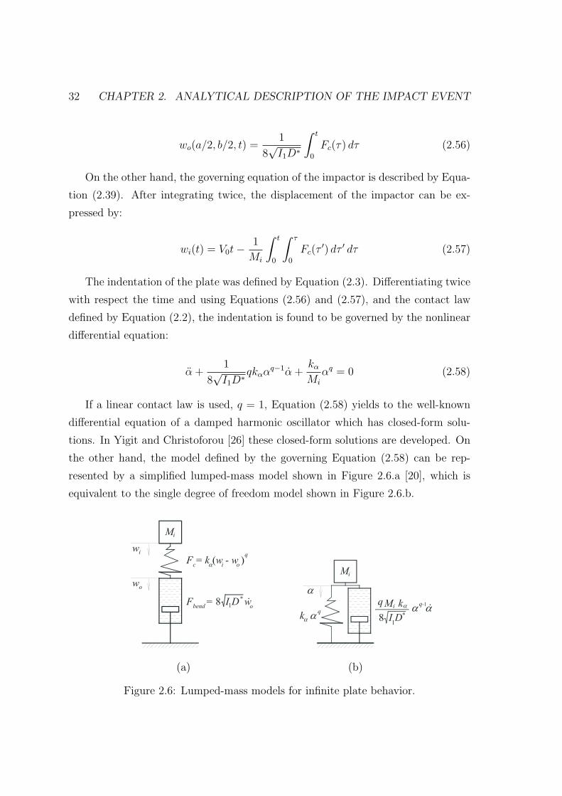
32 CHAPTER 2. ANALYTICAL DESCRIPTION OF THE IMPACT EVENT
wo(a/2, b/2, t) =1
8√I1D∗
∫ t
0
Fc(τ) dτ (2.56)
On the other hand, the governing equation of the impactor is described by Equa-
tion (2.39). After integrating twice, the displacement of the impactor can be ex-
pressed by:
wi(t) = V0t−1
Mi
∫ t
0
∫ τ
0
Fc(τ′) dτ ′ dτ (2.57)
The indentation of the plate was defined by Equation (2.3). Differentiating twice
with respect the time and using Equations (2.56) and (2.57), and the contact law
defined by Equation (2.2), the indentation is found to be governed by the nonlinear
differential equation:
α +1
8√I1D∗
qkααq−1α +
kαMi
αq = 0 (2.58)
If a linear contact law is used, q = 1, Equation (2.58) yields to the well-known
differential equation of a damped harmonic oscillator which has closed-form solu-
tions. In Yigit and Christoforou [26] these closed-form solutions are developed. On
the other hand, the model defined by the governing Equation (2.58) can be rep-
resented by a simplified lumped-mass model shown in Figure 2.6.a [20], which is
equivalent to the single degree of freedom model shown in Figure 2.6.b.
(a) (b)
Figure 2.6: Lumped-mass models for infinite plate behavior.

2.4. ANALYTICAL IMPACT MODELS 33
The governing Equation (2.58) can be expressed in a dimensionless form, which
is more effective in order to analyze the effects of the governing parameters on
the impact behavior. That is because the governing parameters are set on key
dimensionless parameters, yielding to less characterization parameters of the impact
response. This framework can be developed by defining all the basic magnitudes
of the problem (i.e. mass [M ], length [L], and time [T ]) by means of selected
parameters of the impact problem [26, 57]. The chosen definitions are [65]: mass
[M ] = Mi, length [L] = V0[T ], and time [T ] is extracted from the contact stiffness kα
which depends on the selected contact law. Therefore [T ] =(k−1α [M ][L](1−q)
)1/2=(
k−1α MiV
(1−q)0
)1/(1+q)
.
The explained definitions are equivalent to define the variable [L] equal to αmax
[19, 26, 54]. The αmax corresponds to the maximum indentation of the plate (i.e.
when the global response of the plate is neglected, which is called half-space impact).
The expression of αmax is simply found by equating all impact energy with the
indentation energy. Consequently, the impact force is normalized with respect to
the maximum impact force for a half-space behavior. Therefore, the equation of
αmax for a general contact law yields to:
αmax =
(1 + q
2
MiV2
0
kα
)1/(1+q)
(2.59)
The resulting dimensionless differential equation is:
¨α + ζqαq−1 ˙α + αq = 0 (2.60)
where the over bar indicates dimensionless parameters and the initial conditions are
α(0) = 0 and ˙α(0) = 1. All parameters that describe the impact behavior are now
lumped in a single dimensionless parameter ζ. This parameter is defined by:
ζ =1
8√I1D∗
(kαM
qi V
q−10
)1/(1+q)(2.61)
In the bibliography, the ζ parameter is called relative plate mobility [20], inelas-
tic parameter [7, 28], or loss factor [19]. The highest contact force is obtained for
ζ = 0, in which case the plate is very rigid and the problem is reduced to that of an
impact on a half-space impact behavior where the impactor will rebound with the

34 CHAPTER 2. ANALYTICAL DESCRIPTION OF THE IMPACT EVENT
initial velocity V0 [22]. As the impact parameter ζ increases, the contact force his-
tory becomes asymmetrical and the contact duration increases because the flexural
deformation of the target becomes more significant (i.e. the behavior approaches to
a quasi-static response type). Under high values of ζ the model is not appropriate
since the model is affected by the boundary conditions and the global deformation
of the structure.
In Olsson [20] the parameter ζ is defined by introducing the concept of mobility,
C, which is defined as velocity per unit force applied to a component. The mobility
of the plate, Cp, is given by:
Cp =woFbend
=1
8√I1D∗
(2.62)
The impactor mobility, Ci, may be defined from peak (initial) velocity, V0, per
peak load, Fmax for a complete immovable plate (i.e. Cp = 0 and the indentation is
maximum αmax):
Ci =V0
Fmax=
V0
kααqmax
=
(k−1α V 1−q
0
(1 + q
2Mi
)−q)1/(1+q)
(2.63)
By means of the mobility definitions, the ζ parameter can be redefined by the
following expression:
ζ =
(2
1 + q
)q/(1+q)CpCi
(2.64)
The simplified model can be applied until the waves are reflected back from the
boundaries. Equation (2.65) was proposed by Olsson [20], and it gives the position
in polar coordinates r and θ for the leading edge of the n-th wave mode in an
orthotropic plate. Therefore, the simplified model is not suitable if the value given
by this equation is greater than the minimum distance from the impact point to the
boundaries of the plate.
rn(θ) =
(2Dr(θ)D
∗
I1
√D11D22
)1/4√πnt (2.65)
where Dr(θ) is the radial plate bending stiffness in direction θ.

2.4. ANALYTICAL IMPACT MODELS 35
2.4.3 Half-space impact models
When the impactor mass is very small, and the target is fairly stiff, impact does not
produce significant global structure response and can be approximated by impact on
a half-space (i.e. the response is fully local). Then, this behavior can be approached
by single mass-spring-damper model shown in Figure 2.7. The resulting governing
equation is:
Miwi + Fc = 0 (2.66)
where the contact law is defined by Fc = kααq = kαw
qi , and the initial conditions
are wi(0) = 0 and wi(0) = V0.
Figure 2.7: Spring-mass model for half-space impact behavior.
The dimensionless framework described in Yigit and Christoforou [45] defines the
problem magnitudes as [M ] = Mi, [L] = αcr, and [T ] =(k−1α Miα
(1−q)cr
)1/2
. The αcr
term is the yielding indentation for plastic indentation which is defined by Equation
(2.28) (see Section 2.3.3). Using these definitions, the dimensionless form of the
governing Equation (2.66) is:
¨wi + wi = 0 (2.67)
On the other hand, the resulting normalized impact velocity β groups all the
parameters for half-space behavior. Therefore, the β parameter fully characterizes
the half-space behavior and is termed characteristic impact parameter. That is:
β =V0
ωαcr(2.68)
where ω is the contact frequency given as:

36 CHAPTER 2. ANALYTICAL DESCRIPTION OF THE IMPACT EVENT
ω = [T ]−1 =(k−1α Miα
(1−q)cr
)−1/2(2.69)
However, by using the dimensionless framework explained in Section 2.4.2, i.e.
mass [M ] = Mi, length [L] = αmax, and time [T ] =(k−1α Miα
(1−q)max
)1/2
, the β param-
eter remains constant. In particular, for linear contact law q = 1, β parameter is
equal to 1, and for Hertzian contact law q = 3/2, β parameter is equal to (5/4)−1/2.
This result implies that the predicted normalized response given for this behavior is
constant whatever the values of the governing parameters of this behavior. This in-
teresting consideration is used in the impact characterization diagram of Chritoforou
and Yigit [19, 26, 27] which is explained in Section 2.5.
On the other hand, the model defined for wave-controlled impact behavior can
be used in order to describe the half-space behavior. As it has been noted, the
half-space impact behavior will be obtained when the ζ parameter yields to zero.
2.4.4 Quasi-static impact models
For sufficiently large impact times, the response is more or less quasi-static, in the
sense that load and deflection give the same relation as during a static loading.
Based on extensive experimental and computational experience, researchers suggest
that the response is almost quasi-static if the effective mass ratio µ is greater than
a threshold value [66]. This effective mass ratio is given by:
µ =Mi
M∗p
(2.70)
whereMi is the impactor mass andM∗p is the equivalent lumped mass of the structure
which depends on the type of structure and support conditions. For rectangular and
simply supported plates it is set equal to 1/4 of the total plate mass Mp, as can be
deduced from Equation (2.36).
The most complete simplified model for quasi-static behavior description is shown
in Figure 2.8.a [67], where the terms ks, kb and km are the shearing, bending and
membrane stiffness of the plate under static load. The expression of ks, kb and km
are function of the boundary conditions, the shape and the laminate configuration

2.4. ANALYTICAL IMPACT MODELS 37
of the structure. The stiffness values can be obtained experimentally, by using nu-
merical methods, or analytically in cases with simple plate geometries [21]. A list of
stiffness expressions for transverse isotropic plates is done in Sierakowski et al. [68].
(a) (b)
Figure 2.8: (a) Complete and (b) simplified spring-mass models for quasi-static
impact behavior.
The governing equations for each mass by neglecting the gravitational forces are
[67] (Figure 2.8.a):
Miwi + kα (wi − wo)q = 0 (2.71)
M∗p wo + kswo + kbwo + kmw
3o − kα (wi − wo)q = 0 (2.72)
where the initial conditions are wi = wo = 0, wo = 0 and wi = V0. In Olsson [24]
this model is used in conjunction with a delamination force threshold and a critical
energy for delamination growth in order to predict the impact damage initiation and
growth during quasi-static response caused by large mass impactors.
The equivalent plate mass M∗p is negligible when the impactor mass is larger than
twice the total plate mass. By neglecting the plate mass and linearizing the stiffness
km and kα (i.e. linear stiffness k∗m and k∗α), the model yields to the model shown
in Figure 2.8.b [20]. In this case, all stiffness can be lumped to a single stiffness kΣ
which is defined by:

38 CHAPTER 2. ANALYTICAL DESCRIPTION OF THE IMPACT EVENT
kΣ =k∗αkbsmk∗α + kbsm
, where kbsm =
(1
kb+
1
ks
)−1
+ k∗m (2.73)
The governing equation for this case is:
Miwi + kΣwi = 0 (2.74)
where the initial conditions are wi = 0 and wi = V0. More simplified versions are
proposed in the literature, such as models with neglected membrane effects and/or
shear effects [19]. Equation (2.74) can be written in a dimensionless form by using
the magnitude definitions shown in Section 2.4.2 specified for a linear contact law
(i.e. q = 1). That is:
¨wi +
(kbsm
kbsm + k∗α
)wi = 0 (2.75)
2.5 Approaches for impact behavior description
There are approaches in the literature which predict the impact behavior type of
rectangular, flat, and monolithic laminated composite plates. These approaches are
based on simplified analytical models of extreme impact behaviors and develop key
characterization parameters which inform of the behavior type. As it has been noted
in Section 2.2, the behaviors considered are those that yield to Barely Visible Impact
Damage (BVID) if the resulting peak load reaches a designed damage threshold.
Ballistic impact behavior is beyond the scope of the present thesis.
The approaches detailed in this section are the characterization diagram pro-
posed by Christoforou and Yigit [19, 26, 27], and the mass criterion proposed by
Olsson [20]. It should be noted that not all impact cases are adequately character-
ized by the approaches explained at following. This is due to the fact that these
approaches are based on simplified models based on certain hypothesis that may not
be true for certain impact configurations.
2.5.1 Christoforou and Yigit characterization diagram
The characterization impact diagram proposed by Christoforou and Yigit [18, 19,
26, 27] predicts the behavior type, as well as the maximum elastic impact force for

2.5. APPROACHES FOR IMPACT BEHAVIOR DESCRIPTION 39
a wide range of impact cases. The prediction of the maximum impact force is useful
since it can be compared with a damage threshold for damage onset (see Section
2.6).
The construction of the diagram is based on simplified analytical models of the
infinite plate and quasi-static impact behaviors, and uses the dimensionless frame-
work described in Section 2.4.2 (i.e. the normalization with respect to the maximum
indentation αmax). On the other hand, a linearized contact law of the elastic-plastic
contact model proposed in Yigit and Christoforou [45] is used, that results in closed-
form solutions for the impact models.
Infinite plate behavior
The closed-form solutions, Equation (2.76), are the expressions of the normalized
impact force as a function of the relative mobility parameter ζ with q = 1 (see
Equations (2.60) and (2.61)). It should be noted that ζ parameter is changed to
ζ = 2ζw which simplifies the resulting equations:
Fw (t) = α (t) =
exp−ζw t√1− ζ2
w
sin(√
1− ζ2w t)
if ζw < 1
t exp−t if ζw = 11
2√ζ2w − 1
(exp
(−ζw+√ζ2w−1
)t− exp
(−ζw−√ζ2w−1
)t
)if ζw > 1
(2.76)
The dimensionless time at which the maximum impact force occurs can be found
by setting the derivatives with respect to time equal to zero, in Equation (2.76),
yielding:
tw =
arccos
(ζw√
1− ζ2w
)if ζw < 1
1 if ζw = 1
1
2√ζ2w − 1
ln
(ζw +
√ζ2w − 1
ζw −√ζ2w − 1
)if ζw > 1
(2.77)
Then, the maximum normalized impact force can be calculated by replacing
Equation (2.77) into Equation (2.76) as:
40 CHAPTER 2. ANALYTICAL DESCRIPTION OF THE IMPACT EVENT
Fw,max (tw) = α (tw) (2.78)
From Equation (2.78), it is concluded that the infinite plate behavior is function
of only the parameter ζw, because tw only depends on it.
Half-space behavior
As noted in Section 2.4.3, the half-space behavior can be described by the spring-
mass model shown in Figure 2.7. Due to the dimensionless framework used, the
dependence on the characterizing half-space parameter β is avoided and the nor-
malized impact force can be obtained by normalizing Equation (2.66):
Fhs (t) = α (t) = wi (t) = sin t (2.79)
Thus, if an impact response is locally dominated, the maximum normalized im-
pact occurs at time ths = π/2 and this force will be close to the unity Fhs,max = 1.
This development also can be deduced by means of the governing Equation (2.60)
of the wave-controlled impact model and letting the ζw parameter equal to zero.
Quasi-static behavior
The quasi-static behavior is described by the model shown in Figure 2.8.b. Equaling
the linear contact stiffness k∗α to ky (Equation (2.27)), and defining λ = kbsm/ky (i.e.
relative stiffness), the solution of the dimensionless governing Equation (2.75) (see
Section 2.4.4) is:
wi (t) =
√1 + λ
λsin
(√λ
1 + λt
)(2.80)
and the normalized impact force for quasi-static behavior is:
Fq (t) =
√λ
1 + λsin
(√λ
1 + λt
)(2.81)
From Equation (2.81), the maximum normalized impact force occurs at time:

2.5. APPROACHES FOR IMPACT BEHAVIOR DESCRIPTION 41
tq =π
2
√1 + λ
λ(2.82)
and is defined as:
Fq,max =
√λ
1 + λ(2.83)
As Equation (2.83) shows, the maximum normalized impact force for quasi-static
behavior only depends on λ parameter.
Impact characterization diagram
Using the analytical solutions of the extreme cases explained above, a characteriza-
tion diagram can be constructed as shown in Figure 2.9. This diagram represents the
variation of the maximum normalized impact force Fmax as a function of the relative
mobility parameter ζw. For the construction of the diagram, the curve representing
infinite plate behavior is obtained from Equation (2.78), and the horizontal lines
with different values of relative stiffness λ are obtained by using Equation (2.83).
Figure 2.9: Impact characterization diagram (after Christoforou and Yigit [18, 19,
26, 27]), dimensionless maximum force Fmax versus relative mobility ζw.
Four different regions can be identified in the diagram. Impact configurations
which define points in the right part of the diagram behave as quasi-static. For points
which fall close to the red curve behave as infinite plate. Between the quasi-static

42 CHAPTER 2. ANALYTICAL DESCRIPTION OF THE IMPACT EVENT
and the infinite plate behaviors there is a transition zone where the resulting response
is a combination of both behaviors. The curve which represents the boundary of
the quasi-static response is obtained by Fb =√
0.680.68+ζ2w
, as suggested in [26, 66].
Finally, the points that fall close to the maximum dimensionless force F = 1 results
in the half-space behavior, and can be obtained by setting in the simplified models
(infinite plate and quasi-static): ζw = 0 or λ→∞.
In order to demonstrate the validity of the characterization diagram several im-
pact situations covering all behavior type regions were simulated [26]. The simu-
lations were carried out by numerical integration of the complete analytical model
which considers classical laminated plate theory and simply supported boundary
conditions (see Section 2.4.1). As can be seen, the simulations follow reasonably
well the trends of the characterization diagram. In the transition zone, a complete
analytical model is required in order to better describe the response.
Summarizing, the prediction of the behavior type as well as the maximum impact
force for a given impact case can be done by calculating only two key parameters:
λ (i.e. key parameter of quasi-static impact behavior) and ζw (i.e. key parameter of
wave-controlled impact behavior). However, the contribution of structural dynamics
should be included and it can be represented by the relative impactor mass µ given
by Equation (2.70). When different impact situations (respect to their boundary
conditions, materials, size, etc.) with similar key parameters are compared, the
resulting dynamics, behavior type and normalized response are similar [54].
2.5.2 Olsson mass criterion
Olsson [20] developed a criterion for the prediction of the elastic impact behavior of
orthotropic plates. The model is based on the models for infinite plate and quasi-
static extreme behaviors described in Sections 2.4.2 and 2.4.4, respectively. This
criterion demonstrates that the response type under elastic conditions (i.e. prior
to damage onset) depends basically on the impactor/plate mass ratio. In order to
develop the criterion, the dimensionless framework presented in Section 2.4.2 was
also used.
2.5. APPROACHES FOR IMPACT BEHAVIOR DESCRIPTION 43
Small-mass impactor
For small-mass impactor, it is demonstrated that the impact time ti has the following
approximate lower bound [20]:
ti ≥1
4
Mi√I1D∗
(2.84)
The mass of the plate area affected by the first wave, Mp,wave, is approached by:
Mp,wave = πI1r1(0)r1(90) = π2ti√
2I1D∗ (2.85)
where r1(0) and r1(90) are respectively the distances at 0 and 90 directions from
the impact point site to the leading edge of the first wave mode. They are calculated
by means of Equation (2.65).
On the other hand, the largest plate mass which can remain unaffected by the
boundaries, Mp,max, is found by considering the plate area affected when the first
wave mode reaches a boundary. Therefore, it can be defined as:
Mp,max = πI1 min
(D22
D11
)1/4
r2x,min,
(D11
D22
)1/4
r2y,min
(2.86)
where rx,min and ry,min are the distances from the impact to the closest boundary in
the x− (i.e. 0 direction) and y−direction (i.e. 90 direction). Therefore, an impact
located at middle of the panel implies rx,min = a/2 and ry,min = b/2.
By replacing Equation (2.84) into Equation (2.85) and making the ratios respect
the impactor mass, Mi, the condition for small-mass impact (i.e. infinite plate
impact) is approached by:
Mi
Mp,max
≤ Mi
Mp,wave
≤ 2√
2
π2(2.87)
For rectangular plates with leading edges a and b (see Figure 2.5), the term I1
is equal to Mp
ab. Therefore, the condition for small-mass impact can be expressed as:
Mi
Mp
≤ 1√2π
min
a
b
(D22
D11
)1/4
,b
a
(D11
D22
)1/4
(2.88)

44 CHAPTER 2. ANALYTICAL DESCRIPTION OF THE IMPACT EVENT
Large-mass impactor
For large-mass impactor, the model considered is shown in Figure 2.8.b which ne-
glects the lumped plate mass M∗p and considers linear conditions. For this case, the
natural frequency is:
ωi =
√kΣ
Mi
(2.89)
If the lumped plate mass is not neglected, the natural frequency of the plate is
approached by:
ωp =
√kbsmM∗
p
(2.90)
By means of Equation (2.89) the impact time is obtained:
ti = π
√Mi
kΣ
(2.91)
On the other hand, using Equation (2.90) the first vibration mode of the plate
results in:
tp,1 = π
√M∗
p
kbsm(2.92)
Quasi-static response occurs for impact times much longer than the fundamental
vibration period of the plate, which is described by:
ti/tp,1 >> 1 (2.93)
Replacing Equations (2.91) and (2.92) in Equation (2.93), and considering M∗p =
(1/4)Mp, the criterion for quasi-static behavior yields toMi
Mp
>>1
4. A sufficient
condition is:
Mi
Mp
≥ 2 (2.94)

2.6. IMPACT DAMAGE AND ANALYTICAL THRESHOLDS 45
Intermediate-mass impactor
Finally, a complex response occurs for intermediate-mass impactors, which can be
modeled by including the equivalent plate mass M∗p as shown in Figure 2.8.a. There-
fore, the condition for intermediate mass behavior for rectangular plates is:
1√2π
min
a
b
(D22
D11
)1/4
,b
a
(D11
D22
)1/4<Mi
Mp
< 2 (2.95)
2.6 Impact damage and analytical thresholds
The phenomenon of impact damage in laminated composite structures is very com-
plex and difficult to model analytically due to the large variety of damage modes
(matrix cracking, fiber-matrix interface debonding, delamination and fiber breakage)
and to their complex interaction process. The identification of the initiation and
propagation of the damage modes is quite relevant because it will yield information
regarding the residual strength of the structure.
Similarly to the impact response, depending on the impact governing parame-
ters, the resulting damage can be local, global or both [18, 21]. Local impact damage
consists mainly of visible permanent indentation on the contact zone involving fiber
and matrix damage modes, whereas global impact damage consists mainly of invisi-
ble extensive delaminations. The extreme local damage is the complete penetration
of the plate. Associated with these types of damages, there are complicated patterns
of matrix cracks and fiber fractures.
To bridge the analytical prediction of the impact behavior and the onset of
damage, the impact force is typically used and compared with a damage threshold
allowable. Damage occurs if the predicted elastic impact force is greater than a
well-suited threshold for the corresponding dynamic response type [7, 18, 25, 69, 70].
Therefore, the impact force is a key parameter in determining the criticality of an
impact, i.e. the risk for initiating damage.
2.6.1 Matrix cracking
The impact damage process starts with localized matrix cracks and fiber-matrix
interfacial debondings which normally are not detectable neither by the impactor

46 CHAPTER 2. ANALYTICAL DESCRIPTION OF THE IMPACT EVENT
load cells used during impact tests nor using the typical Non-Destructive Inspection
methods (NDI), e.g. ultrasonic techniques. It has been shown by Sjoblom et al. [71]
that the presence of matrix cracks does not dramatically affect the overall laminate
stiffness during an impact event. However, matrix crack tips act as initiation points
for delaminations at interfaces between plies with different fiber orientations. These
delaminations change the local and/or global stiffness of the structure [31].
Two types of matrix cracks can be observed: vertical and oblique cracks (Figure
2.10). Vertical cracks are introduced by the flexural deformation of the plate due to
tensile stresses and consequently they are located at the bottom plies. Therefore,
vertical cracks are typical in impact events that behave as quasi-static. Oblique
cracks are formed by the high transverse shear stresses resulting from the contact
load and the flexural deformation of the plate. These cracks are typically located at
top and middle plies.
(a) (b)
Figure 2.10: Type of matrix cracks in a [0/90/0] laminated composite plate (after
Richardson and Wisheart [30]), (a) longitudinal view and (b) transverse view.
Typically, in thick laminates matrix cracking starts on the impacted face of the
specimen as a result of the high and localized contact stresses. Damage propagates
downward by a succession of intra-ply cracks and interface delaminations, resulting
in a pine tree pattern (Figure 2.11.a). For thin laminates, bending stresses on the
back of the laminate introduce tensile matrix cracks, and damage progresses from the
non-impacted face up toward the impactor yielding a reverse pine tree appearance
(Figure 2.11.b).

2.6. IMPACT DAMAGE AND ANALYTICAL THRESHOLDS 47
(a) (b)
Figure 2.11: Projected damage patterns (after Abrate [7]), (a) pine tree and (b)
reversed pine tree.
Threshold load for vertical matrix crack
A new damage threshold for the prediction of matrix cracking at the outer ply
located at the back face of a rectangular laminated composite plate due to bending
is proposed herein.
The maximum values of the in-plane tensile stresses due to the flexural defor-
mation created by a uniformly distributed static load of radius R, q0 = F tenmc / (πR2),
centered at (x, y, z) = (a/2, b/2,−h/2) in a simply supported, rectangular and or-
thotropic plate (see Figure 2.5), can be approximated by [61]:
(σx)max =8b2
π5R2h2fx(s, Cij, Dij/h
3)F tenmc (2.96)
(σy)max =8b2
π5R2h2fy(s, Cij, Dij/h
3)F tenmc (2.97)
where R is the impactor tip radius and h is the plate thickness. These maximum
in-plane tensile stresses are located at (x, y, z) = (a/2, b/2, h/2), i.e. at the impact
point and at the opposite point at the back face of the plate, and are obtained by
means of the classical laminated plate theory, using the Navier solution for simply
supported plates, and neglecting membrane strains and local deflections. The terms
fx (s, Cij, Dij/h3) and fy (s, Cij, Dij/h
3) are defined respectively as:
fx(s, Cij, Dij/h
3)
= h3
∞∑
m=1
∞∑
n=1
ξ
ϑ
(s2m2C11 + n2C12
)(2.98)
fy(s, Cij, Dij/h
3)
= h3
∞∑
m=1
∞∑
n=1
ξ
ϑ
(s2m2C12 + n2C22
)(2.99)
48 CHAPTER 2. ANALYTICAL DESCRIPTION OF THE IMPACT EVENT
where s = b/a, ξ = 1mn
sin(mπRa
)sin(nπRb
), ϑ = D11m
4s4 + 2(D12 + 2D66)m2n2s2 +
D22n4, and Cij and Dij are respectively the constitutive and bending stiffness com-
ponents of the laminated composite plate calculated by means of the homogenized
engineering constants [72]. Equations (2.98) and (2.99) are valid only for odd values
of m and n. By adding enough terms, the solution of Equations (2.96) and (2.97)
can converge, whereas convergence is not possible for a point load case [61].
The maximum stresses given by Equations (2.96) and (2.97) must be transformed
to the stress components on the back outer ply of the laminate (i.e. (σ1, σ2, σ6)p).
This is done by calculating the strain components of the plate; afterwards, the strain
components are rotated to the local coordinates of the ply (axis 1 is aligned with the
fibers, and axis 2 corresponds to the transverse direction to the fibers); finally, by
means of the constitutive matrix of the ply, the corresponding stresses are obtained.
All these operations are collected in the following equation:
σ1
σ2
σ6
p
= [C]p [T ]γ [S]
(σx)max
(σy)max0
(2.100)
where [C]p is the constitutive matrix of the back outer ply in the ply coordinate sys-
tem, [T ]γ is the rotation matrix of the engineering strains from the plate coordinate
system to the ply coordinate system (see Appendix A), and [S] is the compliance
matrix of the plate in the plate coordinate system (i.e. [S] = [C]−1). Developing
Equation (2.100), the resulting ply stresses are:
(σ1)p =(
(C11)p c2 + (C12)p s
2) (S11 (σx)max + S12 (σy)max
)
+(
(C11)p s2 + (C12)p c
2) (S12 (σx)max + S22 (σy)max
) (2.101)
(σ2)p =(
(C12)p c2 + (C22)p s
2) (S11 (σx)max + S12 (σy)max
)
+(
(C12)p s2 + (C22)p c
2) (S12 (σx)max + S22 (σy)max
) (2.102)
(σ6)p = 2cs (C66)p[(S12 − S11) (σx)max + (S22 − S12) (σy)max
](2.103)

2.6. IMPACT DAMAGE AND ANALYTICAL THRESHOLDS 49
where c = cos(θ), s = sin(θ), and θ is the fiber orientation of the ply respect to the
plate coordinate system.
In addition, the in-situ transverse tensile strength Y isT and the in-situ in-plane
shear strength SisL for an outer ply, which is considered thin enough in comparison
with the whole laminate thickness, can be calculated as [73, 74] (see Chapter 6):
Thin outer ply
Y isT = 1.122
√E2
1− ν12ν21
GIcπhp
SisL = 2
√G12GIIcπhp
(2.104)
where E2, G12 and ν21 are the elastic properties of the ply, hp is the ply thickness, and
GIc and GIIc are respectively the fracture toughness in mode I and mode II. Equa-
tion (2.104) is obtained by applying Linear Elastic Fracture Mechanics (LEFM) for
longitudinal crack growth and assuming a uniform stress state. On the other hand,
the tensile strength and the in-plane shear strength for thick plies are approached to
the values measured from tests on unidirectional laminates, Y isT = YT and SisL = SL.
Under the presence of both in-plane shear and transverse tension, the critical
energy release rate Gc depends on the combined effect of all microscopic energy
absorbing mechanisms such as the creation of a new fracture surface. The LaRC
failure criterion [73–77] is used to predict matrix cracking under multi-axial loading:
(1− g)(σ2)pY isT
+ g
((σ2)pY isT
)2
+
((σ6)pSisL
)2
≤ 1 (2.105)
where g = GIc/GIIc.Replacing the transverse and shear stresses ((σ2)p and (σ6)p) in Equation (2.105),
and the corresponding strengths for thin and thick outer plies, the threshold load
for tensile matrix cracking F tenmc can be calculated by simply taking the maximum
value of the two extreme cases, thin and thick: F tenmc = max (F ten
mc )thin , (Ftenmc )thick.
Threshold load for oblique matrix crack
The stress state at the impact point (x, y, z) = (a/2, b/2,−h/2) is 3D due to the
flexural deformation and the contact load. The in-plane compressive and shear
stresses due to the flexural deformation can be approached in the same way as it

50 CHAPTER 2. ANALYTICAL DESCRIPTION OF THE IMPACT EVENT
is indicated in the previous section for determining a threshold load for vertical
matrix crack on the back outer ply of the laminate. Solutions for the stresses due
to concentrated loads in anisotropic plates are scarce and closed-form solutions are
limited to transversely isotropic plates loaded along their axis of symmetry, and
assuming a Hertzian pressure distribution as well as that the plate is semi-infinite,
i.e. half-space [36, 78]. To approximate in a simplified form the stress state at the
impact point, the superposition of the flexural stresses and the contact stresses of a
half-space plate can be applied as it was shown by Olsson [79].
On the other hand, the maximum through-the-thickness shear stresses due to
the flexural deformation created by a transverse static point load F shmc located at
the center of a simply supported, rectangular and orthotropic plate (see Figure
2.5), can be computed using the 3D stress equilibrium equations [61]. These maxi-
mum stresses are located at the edges and middle plane of the plate (i.e. (σr)max:
(x, y, z) = (0, b/2, 0), and (σq)max: (x, y, z) = (a/2, 0, 0)).
For determining the threshold load for matrix cracking at the impact point or
at the edges of plate, a 3D failure criterion is required. The appearance of matrix
cracks located at these points is not as critical as the matrix cracks located at other
points since the former do not act as crack tips for large delaminations. Therefore,
these matrix cracks do not imply a significant reduction of the residual strength of
the structure, and for this reason a threshold load for these matrix cracks is not
developed here.
Olsson et al. [23] proposed a simple threshold load for matrix cracking due
to the through-the-thickness shear stress created by a static concentrated contact
load. The threshold load is calculated by considering the Hertz distribution of the
contact pressure, and the corresponding maximum value of the shear stress in the
through-the-thickness direction and inside the contact radius. In the same way of
the simplified shear stress field indicated by Davies et al. [69], the distribution of
the through-the-thickness shear stress is assumed parabolical with the maximum
located in the middle plane. The threshold load is defined as:
F shmc =
8√
3
9(πSLh)3/2
√R
Qα
(2.106)
where h is the plate thickness, R is the impactor tip radius, and Qα is the effective

2.6. IMPACT DAMAGE AND ANALYTICAL THRESHOLDS 51
contact modulus (see Equation (2.5)).
2.6.2 Delamination
Delaminations are induced by interlaminar shear stresses which are promoted by
matrix cracks, by stiffness mismatch between the adjacent plies, by the thickness
of the ply (ply clustering), and by the laminate deflection. Increasing any of these
factors will result in an increased mismatch in the bending deformations of adjacent
ply groups with different orientations, yielding to large delaminations.
The study of the stiffness mismatch yields important information regarding the
location, orientation, and size of delaminations. Liu [80] proposed the following
dimensionless mismatch parameter ML for two-layer plates based on the difference
of their bending stiffness respect the global coordinate system of the plate:
ML =Dij (θb)−Dij (θt)
Dij (0b)−Dij (90t )(2.107)
where Dij are the components of the bending stiffness matrix. Each ply is considered
separately, so Dij (θb) is the stiffness of the bottom layer acting alone, and the
subscript t refers to the top layer. While a mismatch coefficient can be defined for
each bending coefficient Dij, usually only D11 is considered.
The mismatch parameter proposed in Equation (2.107) is inadequate for uni-
directional plates since ML is not equal to 0 despite the fact that these laminates
do not have interfaces with mismatched adjacent fiber angles. Moreover, for plates
with more than one interface with mismatched fiber orientations of the adjacent
plies, this parameter is not applicable. To solve these limitations, Morita et al. [81]
proposed a new parameter MM which is calculated as:
MM =1
2π
∫ 2π
0
[∆C11(θ)zi]maxD11(θ)
dθ (2.108)
where ∆C11(θ) is the difference of the in-plane stiffness between the adjacent plies
in direction θ, zi is the through-the-thickness distance from the neutral surface to
the considered interface, and D11(θ) is the bending stiffness of the entire laminate
in the direction θ. The parameter MM is a measure of the maximum bending stress

52 CHAPTER 2. ANALYTICAL DESCRIPTION OF THE IMPACT EVENT
discontinuity given as an integrated quantity with respect to θ. It is considered
empirically that the larger the parameter MM , the larger the impact damage area.
Delaminations only occur at interfaces between plies of different orientation. The
shape of the delamination is generally that of an oblong peanut, where its major
axis follows the orientation of the lower ply at the interface [7, 21]. These shapes are
a result of the shear stress distribution around the surrounding area of the impactor,
of the low interlaminar shear strength along or close to the direction of the fibers,
and of the matrix cracks created by the flexural in-plane stresses [82]. Figure 2.12
shows a typical distribution of these delaminations.
Figure 2.12: Example of peanut shaped delaminations.
There are two different phases during the impact driven delamination process (see
Figure 2.13). Firstly, when the impact force reaches a threshold value Fd, there is
unstable crack propagation leading to instantaneous large delaminated areas. This
often causes the impact force to drop in the response, indicating sudden loss of
stiffness [83]. The threshold load Fd does not physically represent the initiation of
damage, as sub-critical matrix cracks and small delaminations may initiate at lower
forces. Rather, it represents the initial value at which damage can be detected using
the typical NDI methods, and a change in the stiffness properties of the laminate
is expected [31, 59]. Normally, the threshold value is greater for thick laminates
than for thin laminates, as shown in Figure 2.13. Secondly, after unstable crack
growth, the size of the delaminations increase linearly with the force indicating
stable delamination growths. Jackson and Poe [84] suggested the following semi-
empirical formula which relates the maximum delamination size ds and the impact
force F :

2.6. IMPACT DAMAGE AND ANALYTICAL THRESHOLDS 53
ds =1
πSLhF (2.109)
where SL is the interlaminar shear strength and h is the plate thickness.
Figure 2.13: Maximum delamination size as a function of the impact force for plates
with different thickness (after Christoforou [18]).
Figure 2.14 shows a typical profile of the impact force versus time history for
a monolithic laminated composite plate, where the threshold load Fd and the peak
force Fmax are identified. Depending on the impact velocity, Fd can be equal to Fmax.
On the other hand, the identification of Fd is not always clear, due to the effects of
the governing parameters (see Chapter 4), or due to the harmonic resonances of the
impactor, of the load cell or of the plate during the impact event [59].
Figure 2.14: Representative impact force versus time history (after ASTM D7136 /
D7136M [59]).

54 CHAPTER 2. ANALYTICAL DESCRIPTION OF THE IMPACT EVENT
Threshold load for delamination
The criteria for matrix cracking given by Equations (2.105) and (2.106) can be used
as delamination threshold loads assuming that the matrix crack tips act as initiation
points for delaminations in impact events with quasi-static behavior.
A delamination growth criterion for static conditions was derived by Davies et al.
[69, 85]. The model was based on Linear Elastic Fracture Mechanics (LEFM) and as-
sumed that mode II fracture determines delamination growth in a simply supported
circular plate. To simplify the development of the model, static loading conditions
were considered, the laminate was treated as isotropic, only small deflections were
considered (membrane effects are neglected), and the through-thickness distributed
delaminations were collapsed into a single and perfectly circular mid-plane delami-
nation. In detail, the relationship between the out-of-plane displacement wo and an
external point load F statd1 is given by the theory for thin plates as:
wo =3r2
p (1− ν2)
4πEh3F statd1 (2.110)
where E, ν, h, and rp are respectively the elastic modulus, the Poisson ratio, the
thickness, and the radius of the plate. Assuming that the system is linear, it allows
to apply the principle of superposition for the development of the elastic energy of
a plate with a circular mid-plane delamination of radius ac:
U =3r2
p (1− ν2)
8πEh3(F stat
d1 )2 − 3a2
c (1− ν2)
8πEh3(F stat
d1 )2
+2
(3a2
c (1− ν2)
8πE(h2
)3
(F statd1
2
)2) (2.111)
The first term of Equation (2.111) is the elastic energy of the plate without the
delamination. The second term is the energy of a circular plate of radius ac. The last
term is related to the elastic energy of two circular plates of radius ac and height
h/2. Knowing that ∂U∂ac
= 2πacGIIc, the threshold load for a mid-plane circular
delamination is:
F statd1 =
π
3
√8EGIIc1− ν2
h3/2 (2.112)

2.6. IMPACT DAMAGE AND ANALYTICAL THRESHOLDS 55
By letting E/(1 − ν2) = (12D)/h3, where D is the bending stiffness, Equation
(2.112) can be rewritten as:
F statd1 = π
√32DGIIc
3(2.113)
Equations (2.112) and (2.113) show that delamination grows under a constant
load independently of the delamination size. Therefore, an initial flaw is not re-
quired and thus the criterion can be used for the prediction of delamination onset.
In addition, experimental data and finite element simulations indicate that the de-
lamination threshold load is independent of the boundary conditions and of the
in-plane size of the plate [23, 24, 31]. Although the delamination criterion was
derived assuming static loading conditions it may, with a moderate correction fac-
tor, be used for impact responses with dynamic effects, such as in an infinite plate
behavior [23]. Probably, this result is due to fact that F statd1 does not depend on
the in-plane dimensions of the plate, in contrast with the threshold F tenmc developed
in previously. In Davies et al. [86], this criterion was used in conjunction with a
quasi-static, energy-balanced model based on finite element solutions to predict the
threshold impact energy for delamination onset.
A more rigorous solution for an arbitrary number of delaminations located at
same intervals through-the-thickness of the plate was derived by Suemasu and Ma-
jima [87]. The threshold impact load is defined as:
F statdnd
= π
√32DGIIcn+ 1
(2.114)
where n is the number of same thickness plate regions separated by nd = n − 1
same size delaminations. In the work developed by Olsson [24], Equation (2.114) is
used for orthotropic plates by simply changing the isotropic plate stiffness D by the
effective plate stiffness D∗ for orthotropic plates (see Equation (2.55)).
The accumulation process of multiple delaminations was also described by Sue-
masu and Majima [87]. For equally sized multiple delaminations, the energy release
rate is distributed nearly parabolic and symmetric about the middle surface, which
corresponds to the location where the energy release rate reaches its maximum. For
this case, the energy release rates are independent of the delamination size, and the
more delaminations exist, the easier the delamination propagation is. Delaminations

56 CHAPTER 2. ANALYTICAL DESCRIPTION OF THE IMPACT EVENT
of unequal size, they tend to an equal size by the growth of the smaller delaminations
regardless of their location through-the-thickness of the laminate. These conclusions
were obtained from closed-form energy release rate expressions summarized in Table
2.1, and by verifications with finite element analysis.
Table 2.1: Energy release rates for unequal size delaminations [87], where S0 =
n3/(m3 + (n−m)3) − 1, S1 = n2 − S0 − 1, and m is the delamination number
(numbering starts with the deepest back face delamination).
Delamination caseEnergy release rates
mth delamination n− 2 delaminations (average)
One delamination
larger than the othersGII =
F 2
32π2DS0 GII =
F 2
32π2D
S1
n− 2
One delamination
smaller than the
others
GII =F 2
32π2D
6n2
n+ 6GII =
F 2
32π2D
n2 + 2n+ 3
n+ 6
Geometric nonlinear effects on the in-plane stresses becomes significant and must
be considered when the deflection of the plate reaches the order of the plate thickness
or that of the delaminated portions. A numerical Rayleigh-Ritz solution for large
deflections was derived in a later paper of Suemasu and Majima [88]. Membrane
effects increase the threshold load and cause an asymmetrical distribution of the
energy release rate so that the delaminations near the back surface grow faster than
those located elsewhere when the load is increased. Also, geometric non-linearity
implies large impact energies for delaminations to propagate farther. Therefore, the
result using the linear assumption that the more delaminations exist the easier is
their propagation may not be true. Considering the finite bending strength and the
critical perforation load, it can be said that a critical radius of the delaminations
from which delamination propagation is difficult may exist. This critical radius is
function of the interlaminar toughness and of an expected number of delaminations.
Olsson et al. [23] developed a fracture mechanics criterion for dynamic growth
of an arbitrary number nd of delaminations in a transverse isotropic plate. Again,
the delaminations are located at the same intervals through-the-thickness of the
laminate, small deflections are considered, and shear deformation is neglected. The

2.6. IMPACT DAMAGE AND ANALYTICAL THRESHOLDS 57
theory is validated for a wide range of test cases by comparison with 3D finite
element simulations. The threshold impact load is:
F dyndnd
=F statdnd√
1− 7π2
216
≈ 1.213F statdnd
(2.115)
where F statdnd
is the quasi-static threshold delamination load given by Equation (2.114).
The resulting delamination threshold load is about 21% higher than the correspond-
ing quasi-static threshold load.
2.6.3 Permanent indentation
An impact on a laminated composite plate, usually results with a visible permanent
indentation at the impact point as a result of the matrix plasticity, disorder of
the broken fibers, and friction between these fibers and the matrix. Just after the
impact, the permanent indentation has its highest value and gradually its depth is
reduced due to the material relaxation.
The prediction of the threshold load at which permanent indentation initiates
can be approached by the following simple equation:
Find = kyαcr (2.116)
where ky is a linearized stiffness of the elastic-plastic loading phase (Equation (2.27)),
and αcr is the critical indentation as from of it permanent indentation starts and is
defined by Equation (2.28).
The corresponding threshold velocity for permanent indentation can be calcu-
lated by means of a simple energy balance of the simplified quasi-static model de-
scribed in Section 2.4.4 and represented in Figure 2.8.b. Assuming that the impact
energy is used for local and global deformation of the plate, the threshold velocity
yields to:
Vind =αcr
M1/2i
[ky +
k2y
kbsm
]1/2
(2.117)
where kbsm is the plate global stiffness.

58 CHAPTER 2. ANALYTICAL DESCRIPTION OF THE IMPACT EVENT
2.6.4 Fiber failure
Fiber failure generally occurs much later in the fracture process than matrix cracking
and delamination, and it is considered as a precursor of plate perforation. Fiber
failure occurs under the impactor due to locally compressive and shear stresses,
and on the non-impacted face due to tensile bending stresses. More extensive fiber
failure normally occurs in the central part of the delaminated region and appears
to be fairly uniformly through-the-thickness of the laminate. Fiber failure in thin
laminates generally affects more plies and is more extensive than in thick laminates,
indicating the importance of membrane stresses in formation of fiber fracture [21].
2.6.5 Perforation
There are numerous modes of failure in which energy can be dissipated in impacts
that result in complete penetration of the plates. Caprino and Lopresto [89] reported
that the perforation energy depends on the total fiber volume of the plate and on
the impactor tip shape, whereas the architecture of the fibers, the stacking sequence
of the laminate and the type of matrix have no effect. Research into perforation
impact is mainly concentrated on the ballistic range, although perforation can also
occur for other types of impact behavior (see Section 2.2).
Perforation occurs when the fibers reach their critical strain, enabling the im-
pactor to completely penetrate the material. Under this assumption, a conservative
estimate of the quasi-static threshold load for perforation F tenper can be obtained by
simply replacing the in-plane longitudinal stress on the back outer ply (Equation
(2.101)) in the following fiber tensile failure criterion [76]:
(σ1)pXT
≤ 1 (2.118)
where XT is the fiber tensile strength. Therefore, the threshold load for perforation
F tenper yields:
F tenper =
π5R2h2XT
8b2X (2.119)
where X is defined as:
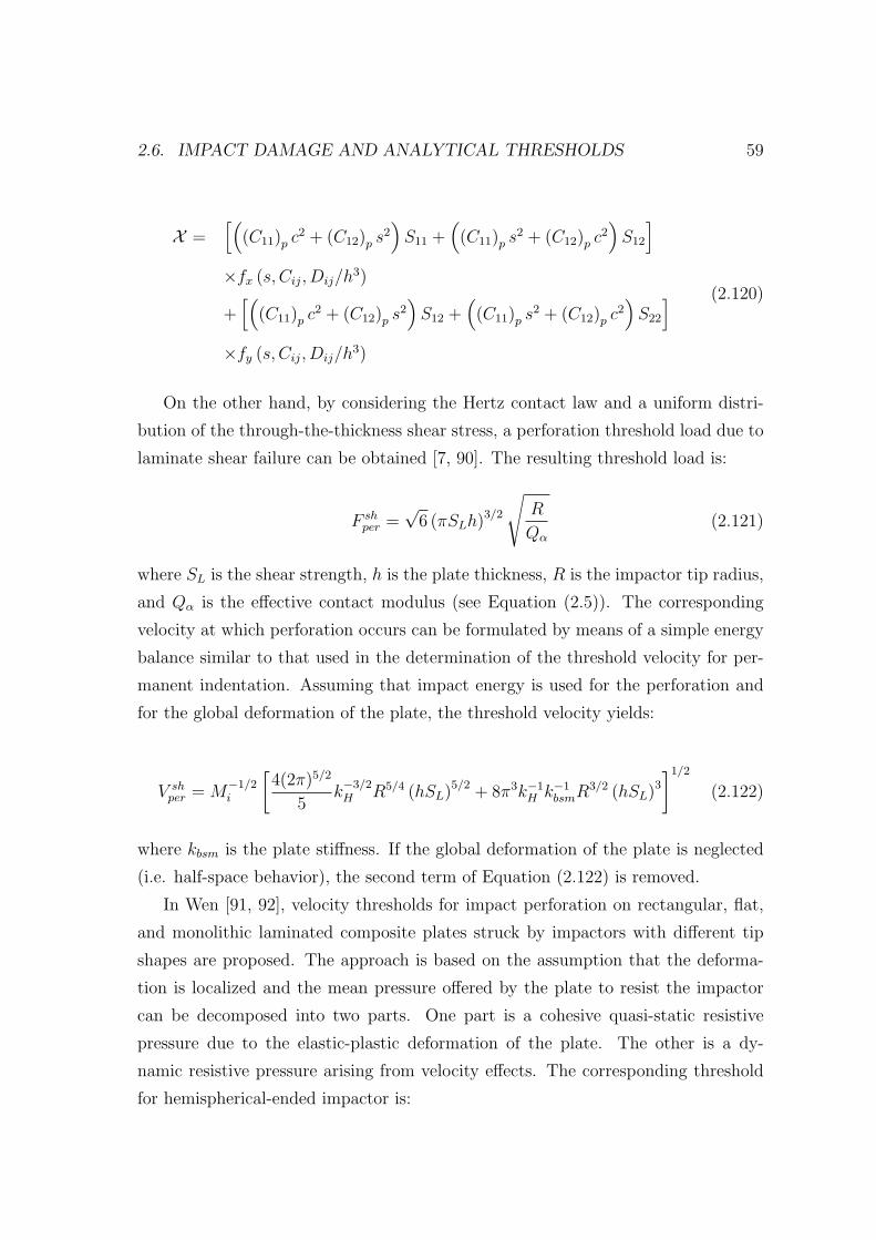
2.6. IMPACT DAMAGE AND ANALYTICAL THRESHOLDS 59
X =[(
(C11)p c2 + (C12)p s
2)S11 +
((C11)p s
2 + (C12)p c2)S12
]
×fx (s, Cij, Dij/h3)
+[(
(C11)p c2 + (C12)p s
2)S12 +
((C11)p s
2 + (C12)p c2)S22
]
×fy (s, Cij, Dij/h3)
(2.120)
On the other hand, by considering the Hertz contact law and a uniform distri-
bution of the through-the-thickness shear stress, a perforation threshold load due to
laminate shear failure can be obtained [7, 90]. The resulting threshold load is:
F shper =
√6 (πSLh)3/2
√R
Qα
(2.121)
where SL is the shear strength, h is the plate thickness, R is the impactor tip radius,
and Qα is the effective contact modulus (see Equation (2.5)). The corresponding
velocity at which perforation occurs can be formulated by means of a simple energy
balance similar to that used in the determination of the threshold velocity for per-
manent indentation. Assuming that impact energy is used for the perforation and
for the global deformation of the plate, the threshold velocity yields:
V shper = M
−1/2i
[4(2π)5/2
5k−3/2H R5/4 (hSL)5/2 + 8π3k−1
H k−1bsmR
3/2 (hSL)3
]1/2
(2.122)
where kbsm is the plate stiffness. If the global deformation of the plate is neglected
(i.e. half-space behavior), the second term of Equation (2.122) is removed.
In Wen [91, 92], velocity thresholds for impact perforation on rectangular, flat,
and monolithic laminated composite plates struck by impactors with different tip
shapes are proposed. The approach is based on the assumption that the deforma-
tion is localized and the mean pressure offered by the plate to resist the impactor
can be decomposed into two parts. One part is a cohesive quasi-static resistive
pressure due to the elastic-plastic deformation of the plate. The other is a dy-
namic resistive pressure arising from velocity effects. The corresponding threshold
for hemispherical-ended impactor is:
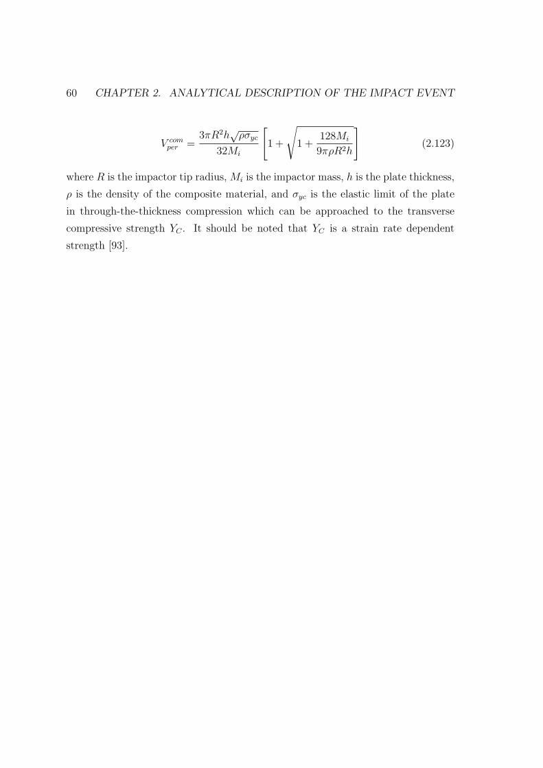
60 CHAPTER 2. ANALYTICAL DESCRIPTION OF THE IMPACT EVENT
V comper =
3πR2h√ρσyc
32Mi
[1 +
√1 +
128Mi
9πρR2h
](2.123)
where R is the impactor tip radius, Mi is the impactor mass, h is the plate thickness,
ρ is the density of the composite material, and σyc is the elastic limit of the plate
in through-the-thickness compression which can be approached to the transverse
compressive strength YC . It should be noted that YC is a strain rate dependent
strength [93].

Chapter 3
Test configurations
3.1 Introduction
In the aeronautical industry, drop-weight impact tests are performed to assess the
damage resistance of a structure. These tests create delaminations which are typi-
cally categorized as Barely Visible Impact Damage (BVID). Delaminations reduce
significantly the compressive strength of the impacted structure. For this reason,
Compression After Impact tests (CAI) are performed in order to assess the damage
tolerance of the structure.
The sequential experimental tasks which are carried out in the present thesis
in order to analyze laboratory coupons are: definition of the impact configura-
tions (i.e. selection of the governing parameters), manufacturing of the specimens,
non-destructive inspections for the detection of manufacturing flaws (e.g. ultra-
sonic techniques), drop-weight impact tests, non-destructive inspections to detect
the BVID, and finally, CAI tests.
This chapter presents the definition of a set of low-velocity impact tests on lam-
inated composite plates which allow the study of the effects of some governing
parameters on the damage resistance. The goal is to obtain a range of different
experimental results that will be used to assess whether the predictions given by
the numerical simulations accurately account the complexity of the impact damage
(see Chapter 7). It should be noted that all studies are focused on the effects of the
governing parameters on the impact damage rather than on the results of the CAI
tests. Furthermore, the description of the CAI test set-up is also explained in detail.
61
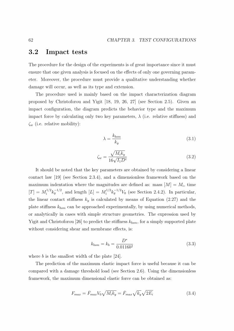
62 CHAPTER 3. TEST CONFIGURATIONS
3.2 Impact tests
The procedure for the design of the experiments is of great importance since it must
ensure that one given analysis is focused on the effects of only one governing param-
eter. Moreover, the procedure must provide a qualitative understanding whether
damage will occur, as well as its type and extension.
The procedure used is mainly based on the impact characterization diagram
proposed by Christoforou and Yigit [18, 19, 26, 27] (see Section 2.5). Given an
impact configuration, the diagram predicts the behavior type and the maximum
impact force by calculating only two key parameters, λ (i.e. relative stiffness) and
ζw (i.e. relative mobility):
λ =kbsmky
(3.1)
ζw =
√Miky
16√I1D∗
(3.2)
It should be noted that the key parameters are obtained by considering a linear
contact law [19] (see Section 2.3.4), and a dimensionless framework based on the
maximum indentation where the magnitudes are defined as: mass [M ] = Mi, time
[T ] = M1/2i k
−1/2y , and length [L] = M
1/2i k
−1/2y V0 (see Section 2.4.2). In particular,
the linear contact stiffness ky is calculated by means of Equation (2.27) and the
plate stiffness kbsm can be approached experimentally, by using numerical methods,
or analytically in cases with simple structure geometries. The expression used by
Yigit and Christoforou [26] to predict the stiffness kbsm, for a simply supported plate
without considering shear and membrane effects, is:
kbsm = kb =D∗
0.0116b2(3.3)
where b is the smallest width of the plate [24].
The prediction of the maximum elastic impact force is useful because it can be
compared with a damage threshold load (see Section 2.6). Using the dimensionless
framework, the maximum dimensional elastic force can be obtained as:
Fmax = FmaxV0
√Miky = Fmax
√ky√
2Ei (3.4)

3.2. IMPACT TESTS 63
where Fmax is the dimensionless maximum elastic force extracted from the impact
characterization diagram by means of the key parameters λ and ζw. The variable
Ei is the impact energy.
3.2.1 Benchmark: ASTM drop-weight impact test
The ASTM test method for measuring the damage resistance of a fiber-reinforced
polymer matrix composite when subjected to a drop-weight impact event (i.e. ASTM
D7136 / D7136M [59]) is taken as a reference in order to fix some of the govern-
ing parameters. Other guidelines for a drop-weight impact test provided by the
aeronautical industry are available (e.g. Airbus AITM1-0010 [94]; Boeing 7260 [95];
NASA ST-1 [96]), however the set-ups are all essentially the same.
The standard is focused on rectangular, flat, and monolithic laminated com-
posite plates with 150mm×100mm in-plane dimensions. If the laminates are man-
ufactured using unidirectional plies, a balanced and symmetric stacking sequence
[(45/0/− 45/90)n]S is defined. The whole number n is selected in such a way that
the cured plate thickness is close to 5mm. The plate stacking sequence is defined
by taking the 0 fiber orientation aligned with the longer in-plane dimension of the
plate.
The specimens are placed over a flat support fixture base with a 125mm×75mm
rectangular cut-out which allows the impactor to contact through the specimen
without interferences (see Figure 3.1.a). Guiding pins are located such that the
specimen can be centrally positioned over the cut-out. The support fixture base has
four rubber-tipped clamps which restrain the specimen during impact and provide a
minimum holding capacity of 1100N. These rubber-tipped points clamp the specimen
at 12.5mm and 6mm from each edge of the open window of the fixture base (see
Figure 3.1.b) [94]. The boundary conditions provided by the clamping system can
be approximated to simply supported [60].
The impact tests are carried out with an impact tester, which includes a guide
mechanism, a rigid clamping system, a drop-weight instrumented impactor, a ve-
locity sensor, and a rebound catcher. The impacts are performed by releasing the
impactor with a selected mass from a desired preset height, and dropped freely
according to the gravitational force and following a guide mechanism. A normal
incidence angle impact occurs at the center of the plate caused by a 16mm diameter

64 CHAPTER 3. TEST CONFIGURATIONS
(a) (b)
Figure 3.1: (a) Impact support fixture; (b) detail of the support area and clamping
points of the specimen.
hemispherical-shaped impactor made of hardened steel. Just prior to impact on the
specimen, a steel flag connected to the impactor is passed through an optical sensor
which triggers the data acquisition system and calculates the initial impact velocity
V0. The velocity is calculated from the distance between two edges of the flag and
the time interval to pass through the sensor. Once impact begins, the contact force
is detected by the force transducer attached to the impactor. The force history is
stored in a computer. Finally, if perforation does not occur, a rebound catcher is
also triggered by the optical sensor so that a re-strike does not occur.
The velocity and displacement history of the impactor, V (t) and wi(t) respec-
tively, can be calculated by integrating once and twice the force history:
V (t) = V0 + gt−∫ t
0
F (t)
Mi
dt (3.5)
wi(t) = w0 + V0t+gt2
2−∫ t
0
(∫ t
0
F (t)
Mi
dt
)dt (3.6)
where V0 is the initial impact velocity, g is the acceleration due to the gravity, t is
the time, and w0 is the impactor position from reference location at time t = 0.

3.2. IMPACT TESTS 65
Additionally, the energy absorbed by the specimen, Ea(t), can be calculated as:
Ea(t) =Mi (V
20 − V (t)2)
2+Migwi(t) (3.7)
The standard suggests testing a sample of 5 specimens using a constant impactor
mass of 5.5kg and a constant impact energy calculated in function of the specimen
thickness:
Ei = CEh (3.8)
where h is the plate thickness and CE is a ratio of the impact energy to the specimen
thickness equal to 6.7J/mm. The reason for defining the impact energy by means
of Equation (3.8) is related to the effects of the support conditions on the impact
damage. When an impact is performed following the standard specifications, the
specimen will develop damage sizes less than half of the unsupported specimen width
(i.e. 38mm), thus avoiding significant interactions of the damage areas with the edge
support conditions.
Tables 3.1 and 3.2 summarize the specifications of the standard regarding the
specimen coupons and the impactor.
Table 3.1: ASTM D7136 / D7136M specifications for the specimen.
Specimen coupons
Shape Flat and rectangular
Thickness h ≈ 5mm
In-plane size at = 150mm × bt = 100mm
Lamina type Unidirectional or woven fabric
Stacking sequence [(45/0/− 45/90)n]S
(for unidirectional laminas)
Boundary conditions Four rubber-tipped clamps
Following the specifications proposed by the standard, using the properties sum-
marized in Table 7.1 for AS4/8552 carbon-epoxy composite material (see Chap-
ter 7), and assuming a ply thickness of hp = 0.184mm, the resulting laminate is

66 CHAPTER 3. TEST CONFIGURATIONS
Table 3.2: ASTM D7136 / D7136M specifications for the impactor.
Impactor
Shape Hemispherical
Radius R = 8mm
Material Steel (60 to 62 HRC)
Mass Mi = 5.5kg
Velocity V0 =
√2 (CEh)
Mi
Incidence impact angle Normal to the plate
[(45/0/− 45/90)3]S with a total nominal thickness h = 4.42mm. This plate thick-
ness defines an impact energy of Ei = 29.6J (see Equation (3.8)) and an impact
velocity of V0 = 3.28ms−1.
The terms required to find the key parameters of the impact characterization
diagram can be respectively calculated as: kbsm by Equation (3.3), ky by Equation
(2.27), I1 by Equation (A.47), and D∗ by Equation (2.55). Using these definitions
and assuming that the effective in-plane dimensions of the plate are a = 125mm and
b = 75mm (see Figure 3.1.b), yield to: λ = 0.71 and ζw = 8.11. These parameters
predict a quasi-static behavior and a maximum dimensionless force of Fmax = 0.65.
Finally, using Equation (3.4), the maximum impact force is Fmax = 14.28kN.
The analytical damage thresholds can be calculated and compared with the
maximum impact force in order to predict qualitatively the damage occurrence. As
it is noted in the standard, matrix cracking and delamination damage are ensured if
all the specifications of the standard are followed. This is demonstrated in Table 3.3,
where the corresponding damage thresholds for matrix cracking and delamination
are below the maximum predicted force.
Furthermore, the maximum load is close to the perforation threshold which in-
dicates that perforation can occur. However, it is difficult to develop perforation
because other damage mechanisms are generated previously so they absorb energy
and avoid the subsequent perforation process.

3.2. IMPACT TESTS 67
Table 3.3: Damage thresholds for AS4/8552 carbon-epoxy composite material.
Damage mechanism Equation Value [kN]
Matrix cracking (2.105) F tenmc = 5.92
(2.106) F shmc = 1.82
Delamination (2.112), using D∗ F statd1 = 5.66
Permanent indentation (2.116) Find = 0.33
Perforation (2.119) F tenper = 13.98
3.2.2 Selected studies: fixed and variable parameters
Taking as a reference the standard for drop-weight impact test [59], different ex-
perimental studies will be performed. All these studies will be focused mainly on
the damage onset which produces a significant reduction on the structure stiffness
and/or residual strength, i.e. Fd (see Figure 2.14).
The variables selected in order to study their effects are: the ply thickness hp
(ply clustering), the laminate thickness h, stacking sequence, the impactor mass Mi
and the impact velocity V0. The variation of these parameters yield to three main
studies: effect of ply thickness (clustering), effect of the mismatch angles of the
plies, and effect of the laminate thickness. As will be demonstrated in the following
sections, all these studies are under quasi-static impact behavior. Therefore, the
prediction of the maximum elastic impact force can also be obtained by means of
Equation (2.83).
For all laminates, the composite material used is AS4/8552 carbon-epoxy uni-
directional pre-preg. The properties of the material are summarized in Table 7.1
(see Chapter 7). It should be noted that for the calculation of the ply thickness,
the corresponding cured value of the laminate thickness will be used (known after
specimen manufacturing).
All the impact tests described below are performed using a commercially avail-
able CEAST Fractovis Plus instrumented impact drop-weight tower. The impact
tester is equipped with a load cell of 22kN attached to the impactor, an automatic
pneumatic rebound brake system, and a clamping system with a holding capacity
of 3000N at each of the four clamping points (see Figure 3.2).

68 CHAPTER 3. TEST CONFIGURATIONS
(a) (b)
Figure 3.2: Detail of the clamping system, (a) without specimen and (b) with spec-
imen.
Finally, the non-destructive inspections before and after impact will be performed
by the C-scan ultrasonic technique, which gives the projected damaged areas over the
structure thickness. Additionally, the measurements of the dent-depth are performed
by means of a Mitutoyo 3D coordinate measuring machine. It should be noted that
not all the impacted specimens are selected for the dent-depth measurements.
Effect of ply thickness (clustering)
Ply clustering was found to reduce the damage resistance of a laminate [60]. Stacking
plies with the same fiber orientation increases the interlaminar shear stresses at the
adjacent interfaces due to the increased difference in the bending stiffness of the ply
groups. This increase in stress, in turn, leads to larger delaminations.
Ply clustering also reduces the number of interfaces available for delamination,
because delamination typically occurs at interfaces with different fiber orientations.
Reducing the number of locations available for delamination will increase the de-
lamination size at the remaining interfaces [97, 98], since delamination acts as an
energy dissipating mechanism during the impact event.
The transverse tensile and shear strengths of a ply are function of the ply thick-
ness, of the ply position in the laminate, and of the fiber orientation of the adjacent
plies. This is called the in-situ effect. Since matrix cracks act as initiation points
for delaminations, the in-situ effect must be considered for a proper analysis of the
ply clustering effect.
The effect of ply clustering on the damage tolerance, assessed by means of the

3.2. IMPACT TESTS 69
residual compressive load, is not yet fully clear. In fact, the compressive strength
decreases if the plate bending stiffness is reduced. In addition, the laminate bending
stiffness decreases if the size of the delaminations created by impact are large (i.e.
when clustering is increased) but also when the number of delamination planes is
increased (i.e. when clustering is reduced). Therefore, given these counteracting
effects, it is difficult to assess whether ply clustering reduces the damage tolerance
of a structure.
The stacking sequences proposed for this study are [(45/0/− 45/90)4]S,
[(452/02/− 452/902)2]S, and [454/04/− 454/904]S (in the following, these laminates
are respectively identified as L02, L03, and L04). All laminates have the same plate
thickness h because an equal number of plies is used (i.e. 32 plies; h = 5.8mm).
However, the clusterings hp are different (i.e. L02: hp = hpp, L03: hp = 2hpp, and
L04: hp = 4hpp, where hpp is the thickness of a single pre-preg ply), yielding to
different number of interfaces for delamination (i.e. L02: nd = 30, L03: nd = 14,
and L04: nd = 6).
Three different impact energies are considered: 38.6J, 28.6J and 19.3J. Given
that the impactor mass is kept constant at 5kg, the different energies also enable the
study of the effects of velocity. In detail, Table 3.4 shows the impact configurations
for all the laminates. Since the repeatability of the impact test is quite good (see
Chapter 4), a sample of less than three specimens is used for some cases.
Table 3.4: Impact configurations for laminates: L02, L03 and L04.
Specimen name Impact energy [J] Impactor mass [kg] Impact velocity [ms−1] Drop height [mm]
L0x -S01
38.6 5 3.93 787.5L0x -S02
L0x -S03
L0x -S04 28.6 5 3.38 582.5
L0x -S0519.3 5 2.78 394.0
L0x -S06
Using the material properties summarized in Table 7.1, the resulting key pa-
rameters of the impact characterization diagram are: λ = 1.62 and ζw = 4.48 for
laminate L02, λ = 1.60 and ζw = 4.50 for laminate L03, and λ = 1.55 and ζw = 4.58

70 CHAPTER 3. TEST CONFIGURATIONS
for laminate L04. Since the key parameters are independent of the impact veloc-
ity, the resulting values are constant for each laminate at any impact energy (see
Equations (3.1) and (3.2)). Additionally, the key parameters are almost equal for all
laminates due to the fact that the stiffness of the laminates is similar. Therefore, the
dimensional elastic response of the laminates for each impact energy is also expected
to be similar.
Introducing the key parameters in the impact characterization diagram, a quasi-
static behavior and a maximum dimensionless force of Fmax = 0.78 are predicted for
all the laminates. The dimensionless force yields to the following maximum elastic
impact forces for each impact energy: Fmax = 19.8kN for Ei = 38.6J, Fmax = 17.1kN
for Ei = 28.6J, and Fmax = 14.0kN for Ei = 19.3J.
Finally, the damage thresholds explained in Section 2.6 are summarized in Table
3.5. Again, these thresholds are constant for each impact energy since no dependence
with velocity is considered in the formulations. Comparing the threshold loads with
the maximum elastic impact forces, the occurrence for damage can be analyzed
easily.
Table 3.5: Damage thresholds for laminates: L02, L03 and L04.
Damage mechanism EquationValues [kN]
L02 L03 L04
Matrix cracking (2.105) F tenmc : 10.34 (thin) 7.20 (thin) 4.92 (thin)
(2.106) F shmc: 2.74 2.74 2.74
Delamination (2.112), using D∗ F statd1 : 8.53 8.49 8.34
(2.114), using D∗ F statdnd
: 2.61 3.68 5.11
(2.115), using D∗ F dynd1 : 10.35 10.30 10.11
(2.115), using D∗ F dyndnd
: 3.17 4.46 6.19
Permanent indentation (2.116) Find: 0.33 0.33 0.33
Perforation (2.119) F tenper : 24.23 23.88 23.16
The most significant damage threshold loads are the ones which indicate impor-
tant reductions on the plate stiffness and/or strength. Basically, these thresholds
are given by Equations (2.105) and (2.112) (i.e. F tenmc and F stat
d1 , respectively). The
first gives a value for matrix cracking on the back outer ply which can create an

3.2. IMPACT TESTS 71
elongated delamination at the first interface from the back face of the plate. The
second gives a threshold for a circular mid-plane delamination.
As shown in Table 3.5, for laminate type L02 the first delamination appears
in the mid-plane of the plate (Fd = F statd1 ), and for laminate types L03 and L04
the delamination is located on the back face (Fd = F tenmc ). Figure 3.3 shows these
threshold loads as a function of the ply thickness on a logarithmic scale. Only F tenmc
for thin plies depends on the ply thickness (see Equation (2.104)). The solid gray
line shows the trend of the analytical threshold load in function of the ply thickness
for the laminates considered.
10−1
100
104
hp [mm]
Fd
[N]
L02
L03
L04
F statd1 ∝
(h1.5
)
Thin: F tenmc ∝
(h2
h12p
)
Thick: F tenmc ∝
(h2
)
− 12
Figure 3.3: Analytical threshold load trend in function of hp, for laminates L02, L03
and L04. The damage threshold F tenmc for laminates with thin plies is computed from
the stresses of laminate type L03.
Furthermore, it is predicted that perforation will not occur for any impact energy
because all the maximum elastic forces are below the perforation threshold.
Finally, the values of the mismatch parameter proposed by Morita et al. [81]
(see Equation (2.108)) for each laminate are: MM = 0.270mm−2 for L02, MM =
0.235mm−2 for L03, and MM = 0.198mm−2 for L04. The mismatch parameter
provides information about the effects of the mismatch interface angles of the plies
on the resulting projected delamination area. It is considered that the larger the
parameter MM is, the larger the projected delamination area is. The results obtained

72 CHAPTER 3. TEST CONFIGURATIONS
indicate that the laminate with thin plies will have larger projected delamination
area than that of the laminate with thick plies. However, this deduction is not
valid because it is expected that laminate L04 will have larger delaminations due to
the reduced number of available interfaces for delamination. Therefore, the Morita
parameter is not suitable to compare different stacking sequences to predict the
largest resulting delamination area.
Effect of ply mismatch angle at interfaces
The mismatch angle of an interface is the difference in the fiber orientation of the
adjacent plies. Increasing the mismatch angle increases the stress concentration at
the interface due to an increased difference in the bending stiffness. Therefore, the
damage resistance can be reduced if the mismatch angle is increased because larger
delaminations are expected. For this reason, the damage tolerance is also expected
to be reduced.
For this study, the laminate type L02 presented in previous study is compared
with a new laminate [(0/90)9]S (in the following, it is identified as L06). As it can
be seen, laminate L06 has a stacking sequence with increased mismatch angles in
comparison with laminate L02. Laminates L02 and L06 have practically equal cured
ply thickness hp, but different laminate thickness h since more plies are used for L06
(i.e. L02: h = 5.8mm and L06: h = 6.8mm).
The impact configurations considered are the same as the described ones for
ply clustering study. Accordingly, three different impact energies are defined 38.6J,
28.6J and 19.3J, with a constant impactor mass of 5kg (see Table 3.4). Therefore,
the predictions for laminate type L02 given in previous study can be reused herein.
Using the material properties summarized in Table 7.1, the resulting key param-
eters of the impact characterization diagram for laminate type L06 are: λ = 2.52
and ζw = 3.31. Introducing the key parameters in the impact characterization dia-
gram, a quasi-static behavior and a maximum dimensionless force of Fmax = 0.85 are
expected for all the impact energies. The dimensionless force yields to the following
maximum elastic impact forces: Fmax = 21.4kN for Ei = 38.6J, Fmax = 18.4kN for
Ei = 28.6J, and Fmax = 15.1kN for Ei = 19.3J.
Table 3.6 summarizes the main damage threshold loads. The significant first
damage for laminate L06 is Fd = F statd1 which predicts a circular mid-plane delam-

3.2. IMPACT TESTS 73
ination. In addition, it should be noted that the threshold load F tenmc is close to
F statd1 . Therefore, the first drop in the impact load history may be triggered by a
combination of both delamination types.
Finally, it is predicted that perforation will not occur for any impact energy
because all the maximum elastic forces are below the perforation threshold.
Table 3.6: Damage thresholds for laminate L06.
Damage mechanism Equation Values [kN]
Matrix cracking (2.105) F tenmc : 11.26 (thin)
(2.106) F shmc: 3.47
Delamination (2.112), using D∗ F statd1 : 10.65
(2.114), using D∗ F statdnd
: 3.07
(2.115), using D∗ F dynd1 : 12.92
(2.115), using D∗ F dyndnd
: 3.73
Permanent indentation (2.116) Find: 0.33
Perforation (2.119) F tenper : 37.16
Effect of the laminate thickness
Another proposed study is to analyze the effects of the laminate thickness on the
damage resistance. Modifying the plate thickness and the impactor mass, the be-
havior of an impact can be local or global dominated. Because of that, the resulting
damage mechanisms as well as their extensions can vary. For instance, in thick lami-
nates, the delaminations initiate close to the loaded surface since contact stresses are
high. However, in thin laminates, the delaminations initiate close to the mid-plane
since contact stresses are negligible. In addition, thin laminates stand large global
bending deflections which often generate, at a certain point, geometric nonlinear ef-
fects, i.e. membrane effects. These effects stiff the impact response of the structure
because the stiffness evolves from bending to axial.
On the other hand, it is obvious that the damage tolerance is also improved if
the laminate thickness is increased. However, the resulting structures are heavier
and more expensive.

74 CHAPTER 3. TEST CONFIGURATIONS
For this study, the laminate type L02 presented in the previous studies is com-
pared with two new laminates: [(45/0/− 45/90)2]S and [(45/0/− 45/90)6]S (in the
following, they are identified as L01 and L05, respectively). As it can be verified,
the stacking sequences are equal but the number of repeated ply groups are differ-
ent, yielding to three different laminate thicknesses (i.e. L01: h = 3.0mm, L02:
h = 5.8mm, and L05: h = 8.8mm).
The impact configurations considered for laminates L01 and L05 are respectively
summarized in Tables 3.7 and 3.8 (see Table 3.4 for the configurations of the laminate
type L02). The comparable cases of impact energy which allow to analyze the effects
of laminate thickness are: 19.3J for laminates L01 and L02, and 38.6J for laminates
L01, L02 and L05. For both cases of energy, the impactor mass is kept constant and
equal to 5kg.
Table 3.7: Impact configurations for laminate type L01.
Specimen name Impact energy [J] Impactor mass [kg] Impact velocity [ms−1] Drop height [mm]
L01-S01 38.6 5 3.93 787.5
L01-S0219.3 5 2.78 394.0
L01-S03
L01-S0419.3 6 2.54 328.9
L01-S05
L01-S06 12.0 2 3.46 610.4
Table 3.8: Impact configurations for laminate type L05.
Specimen name Impact energy [J] Impactor mass [kg] Impact velocity [ms−1] Drop height [mm]
L05-S0138.6 5 3.93 787.5
L05-S02
L05-S0357.8 6 4.39 982.6
L05-S04
L05-S0557.9 15 2.78 394.0
L05-S06
Besides the configurations considered for the study of the laminate thickness,
Tables 3.7 and 3.8 describe other impact configurations for laminates L01 and L05,

3.2. IMPACT TESTS 75
respectively. These configurations allow to analyze the effects of changing the im-
pactor mass and the impact velocity but keeping constant the impact energy. In
detail, this study is performed by means of: specimens S02 and S03 (Mi = 5kg)
compared with S04 and S05 (Mi = 6kg) for laminate L01, and specimens S03 and
S04 (Mi = 6 kg) compared with S05 and S06 (Mi = 15kg) for laminate L05. In
addition, the impact configuration of specimen L01-S06 is used in order to analyze
if the resulting damage behavior is more localized than other configurations with
larger impactor mass.
Using the material properties summarized in Table 7.1, the resulting key pa-
rameters of the impact characterization diagram and the resulting maximum elastic
impact forces are summarized in Table 3.9 for laminate L01, and in Table 3.10 for
laminate L05.
Table 3.9: Maximum elastic impact force predictions for laminate type L01.
Specimen Mi [kg] λ ζw Fmax V0 [ms−1] Fmax [kN]
L01-S01 5 0.22 16.82 0.43 3.93 10.8
L01-S025 0.22 16.82 0.43 2.78 7.6
L01-S03
L01-S046 0.22 18.42 0.43 2.54 7.6
L01-S05
L01-S06 2 0.22 10.64 0.43 3.46 6.0
Table 3.10: Maximum elastic impact force predictions for laminate type L05.
Specimen Mi [kg] λ ζw Fmax V0 [ms−1] Fmax [kN]
L05-S015 5.67 1.94 0.92 3.93 23.32
L05-S02
L05-S036 5.67 2.13 0.92 4.39 28.5
L05-S04
L05-S0515 5.67 3.36 0.92 2.78 28.5
L05-S06

76 CHAPTER 3. TEST CONFIGURATIONS
Table 3.11 summarizes the main damage threshold loads for laminates L01 and
L05. Perforation damage clearly will occur for specimen L01-S01 because the maxi-
mum elastic impact force is higher than the perforation threshold load. Additionally,
specimens from L01-S02 to L01-S05 (i.e. with an impact energy of 19.3J), the max-
imum load is close to the perforation threshold which indicates that perforation can
also occur. In reality, it is difficult to develop perforation in these specimens because
other damage mechanisms are generated previously so they absorb energy and avoid
the subsequent perforation process. Therefore, except for specimen L01-S01, it is
expected that all impact configurations of laminate L01 will develop a first drop in
the impact load history produced by a narrow and elongated delamination at the
first interface from the back face of the plate (Fd = F tenmc ). On the other hand, perfo-
ration will not occur for any impact configuration of laminate type L05. Moreover,
the significant first damage for laminate L05 is Fd = F statd1 . Thus, it is expected
that the first drop in the impact load histories is produced by a circular mid-plane
delamination as it was also predicted for laminate type L02.
Table 3.11: Damage thresholds for laminates: L01 and L05.
Damage mechanism EquationValues [kN]
L01 L05
Matrix cracking (2.105) F tenmc : 2.68 (thin) 23.80 (thin)
(2.106) F shmc: 1.02 5.11
Delamination (2.112), using D∗ F statd1 : 3.16 15.97
(2.114), using D∗ F statdnd
: 1.37 3.99
(2.115), using D∗ F dynd1 : 3.83 19.37
(2.115), using D∗ F dyndnd
: 1.66 4.84
Permanent indentation (2.116) Find: 0.33 0.33
Perforation (2.119) F tenper : 6.39 56.04
As a summary of the analytical threshold loads for all the laminates described in
the previously proposed studies, Figure 3.4 shows the trends of these loads in func-
tion of the ply thickness on a logarithmic scale. The predicted critical values have
been divided by h2 in order to keep constant the profiles for matrix cracking on the
back outer ply for each stacking sequence type (i.e. type TI: [(45x/0x/− 45x/90x)n]S;
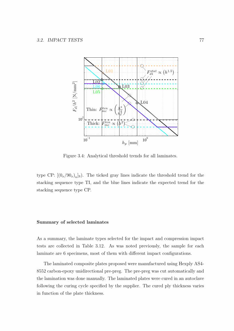
3.2. IMPACT TESTS 77
10−1
100
102
hp [mm]
Fd/h
2[N
/mm
2]
L01
L02L03
L04
L05L06
F statd1 ∝
(h1.5
)
Thin: F tenmc ∝
(h2
h12p
)
Thick: F tenmc ∝
(h2
)
Figure 3.4: Analytical threshold trends for all laminates.
type CP: [(0x/90x)n]S). The ticked gray lines indicate the threshold trend for the
stacking sequence type TI, and the blue lines indicate the expected trend for the
stacking sequence type CP.
Summary of selected laminates
As a summary, the laminate types selected for the impact and compression impact
tests are collected in Table 3.12. As was noted previously, the sample for each
laminate are 6 specimens, most of them with different impact configurations.
The laminated composite plates proposed were manufactured using Hexply AS4-
8552 carbon-epoxy unidirectional pre-preg. The pre-preg was cut automatically and
the lamination was done manually. The laminated plates were cured in an autoclave
following the curing cycle specified by the supplier. The cured ply thickness varies
in function of the plate thickness.

78 CHAPTER 3. TEST CONFIGURATIONS
Table 3.12: Selected laminates.
Name Stacking sequence Number of pliesNumber of interfaces Cured ply Cured plate
for delamination (nd) thickness (hpp) [mm] thickness (h) [mm]
L01 [(45/0/− 45/90)2]S 16 14 0.1875 3.0
L02 [(45/0/− 45/90)4]S 32 30 0.18125 5.8
L03 [(452/02/− 452/902)2]S 32 14 0.18125 5.8
L04 [454/04/− 454/904]S 32 6 0.18125 5.8
L05 [(45/0/− 45/90)6]S 48 46 0.1833 8.8
L06 [(0/90)9]S 36 34 0.1889 6.8
3.3 Compression after impact tests (CAI)
The Compression After Impact test (CAI) is performed to obtain the compressive
residual strength of drop-weight impacted laminates. This is often called the study of
damage tolerance since it refers to the experimental determination or the numerical
prediction of the residual mechanical properties of the damaged structure [7].
Compressive loading causes buckling of sub-laminates in the Barely Visible Im-
pact Damage (BVID) region which forces opening delaminations and then allowing
the damage to propagate from the initial state until the subsequent failure of the
structure. Figure 3.5 shows different buckling modes which can be done during the
CAI test.
Figure 3.5: Buckling modes of delaminated plates in compression (after Davies and
Olsson [21]).
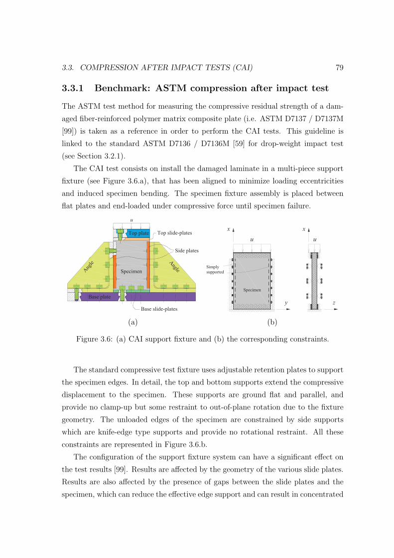
3.3. COMPRESSION AFTER IMPACT TESTS (CAI) 79
3.3.1 Benchmark: ASTM compression after impact test
The ASTM test method for measuring the compressive residual strength of a dam-
aged fiber-reinforced polymer matrix composite plate (i.e. ASTM D7137 / D7137M
[99]) is taken as a reference in order to perform the CAI tests. This guideline is
linked to the standard ASTM D7136 / D7136M [59] for drop-weight impact test
(see Section 3.2.1).
The CAI test consists on install the damaged laminate in a multi-piece support
fixture (see Figure 3.6.a), that has been aligned to minimize loading eccentricities
and induced specimen bending. The specimen fixture assembly is placed between
flat plates and end-loaded under compressive force until specimen failure.
(a) (b)
Figure 3.6: (a) CAI support fixture and (b) the corresponding constraints.
The standard compressive test fixture uses adjustable retention plates to support
the specimen edges. In detail, the top and bottom supports extend the compressive
displacement to the specimen. These supports are ground flat and parallel, and
provide no clamp-up but some restraint to out-of-plane rotation due to the fixture
geometry. The unloaded edges of the specimen are constrained by side supports
which are knife-edge type supports and provide no rotational restraint. All these
constraints are represented in Figure 3.6.b.
The configuration of the support fixture system can have a significant effect on
the test results [99]. Results are affected by the geometry of the various slide plates.
Results are also affected by the presence of gaps between the slide plates and the
specimen, which can reduce the effective edge support and can result in concentrated
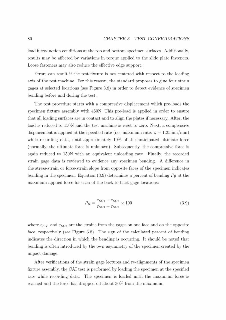
80 CHAPTER 3. TEST CONFIGURATIONS
load introduction conditions at the top and bottom specimen surfaces. Additionally,
results may be affected by variations in torque applied to the slide plate fasteners.
Loose fasteners may also reduce the effective edge support.
Errors can result if the test fixture is not centered with respect to the loading
axis of the test machine. For this reason, the standard proposes to glue four strain
gages at selected locations (see Figure 3.8) in order to detect evidence of specimen
bending before and during the test.
The test procedure starts with a compressive displacement which pre-loads the
specimen fixture assembly with 450N. This pre-load is applied in order to ensure
that all loading surfaces are in contact and to align the plates if necessary. After, the
load is reduced to 150N and the test machine is reset to zero. Next, a compressive
displacement is applied at the specified rate (i.e. maximum rate: u = 1.25mm/min)
while recording data, until approximately 10% of the anticipated ultimate force
(normally, the ultimate force is unknown). Subsequently, the compressive force is
again reduced to 150N with an equivalent unloading rate. Finally, the recorded
strain gage data is reviewed to evidence any specimen bending. A difference in
the stress-strain or force-strain slope from opposite faces of the specimen indicates
bending in the specimen. Equation (3.9) determines a percent of bending PB at the
maximum applied force for each of the back-to-back gage locations:
PB =εSG1 − εSG3
εSG1 + εSG3
× 100 (3.9)
where εSG1 and εSG3 are the strains from the gages on one face and on the opposite
face, respectively (see Figure 3.8). The sign of the calculated percent of bending
indicates the direction in which the bending is occurring. It should be noted that
bending is often introduced by the own asymmetry of the specimen created by the
impact damage.
After verifications of the strain gage lectures and re-alignments of the specimen
fixture assembly, the CAI test is performed by loading the specimen at the specified
rate while recording data. The specimen is loaded until the maximum force is
reached and the force has dropped off about 30% from the maximum.

3.3. COMPRESSION AFTER IMPACT TESTS (CAI) 81
3.3.2 Resources used and specimen instrumentation
In the present thesis, all CAI tests are performed using an Instron-4208 electro-
mechanic universal testing machine with a load cell of 300kN. The fixture support
used follows the ASTM specifications (see Figure 3.7).
(a) (b) (c)
Figure 3.7: CAI test fixture: (a) base support, (b) top support adapted for the
crosshead test machine, and (c) whole fixture.
It should be noted that not all the specimens described in the impact studies
were tested for CAI. A suitable sample of the impacted specimens was selected.
The instrumentation of the specimens is composed by: two displacement trans-
ducers (LVDT) which are used to measure the out-of-plane displacement on two
points of the non-impacted face of the specimen, and four back-to-back strain gages
(SG). The LVDT’s allow to evidence the buckling mode at one face and are lo-
cated at the specimen points indicated in Figure 3.8. The strain gages are used
to detect evidence of specimen bending during the test and are located at 25mm
from each specimen edge (see Figure 3.8). Therefore, the results obtained are the
applied force, the crosshead displacement, the strain data from the gages and the
out-of-plane displacement given by the LVDT’s.
In addition, for some CAI tests the Digital Image Correlation (DIC) method is
used to analyze the impacted face of the specimen (GOM ARAMIS software and
measurement system (version 6.02)). This method provides the measurement of
the 3D displacement field of the surface of interest of an object, generated when
this is submitted to an external loading. The surface to be analyzed must have
a textured pattern in which the light intensity, reflected on the surface, will vary
continuously with a suitable contrast. Therefore, a speckle pattern is created by
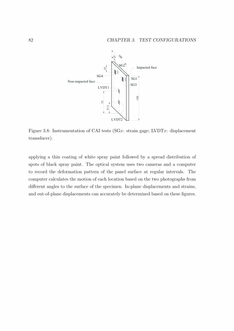
82 CHAPTER 3. TEST CONFIGURATIONS
Figure 3.8: Instrumentation of CAI tests (SGx: strain gage; LVDTx: displacement
transducer).
applying a thin coating of white spray paint followed by a spread distribution of
spots of black spray paint. The optical system uses two cameras and a computer
to record the deformation pattern of the panel surface at regular intervals. The
computer calculates the motion of each location based on the two photographs from
different angles to the surface of the specimen. In-plane displacements and strains,
and out-of-plane displacements can accurately be determined based on these figures.

Chapter 4
Experimental results
4.1 Introduction
In this chapter, the experimental results of the configurations explained in Chapter 3
are shown and discussed in detail. Moreover, comparisons between the experimental
results and the analytical predictions are also analyzed.
The experimental results comprise the data from the impact tests, non-destructive
inspections (NDI) and compression after impact (CAI) tests. It should be noted that
for test configurations with a sample greater than one specimen, the mean values are
used. The C-scan inspections performed before impact are not shown here because
all specimens were not shown manufacturing flaws. Finally, not all the specimens
described in the impact studies were tested for CAI, a sample of the impacted spec-
imens was selected.
The content of this chapter is structured according to the three main proposed
studies, which are: effect of the ply thickness (clustering), effect of the mismatch
angles of the plies, and effect of the laminate thickness.
83

84 CHAPTER 4. EXPERIMENTAL RESULTS
4.2 Effect of ply thickness (clustering)
4.2.1 Impact tests
Impact force versus time
In order to illustrate the excellent repeatability of the impact tests, Figures 4.1
and 4.2 show the evolutions of the impactor reaction force for repeated impact
configurations of laminates L02 and L04, respectively. Therefore, for configurations
with more than one specimen, the mean value is used.
0 1 2 3 4 50
2000
4000
6000
8000
10000
12000
14000
16000
Time [ms]
For
ce [N
]
L02−S01L02−S02L02−S03
0 1 2 3 40
2000
4000
6000
8000
10000
12000
Time [ms]
For
ce [N
]
L02−S05L02−S06
(a) (b)
Figure 4.1: Impact force histories of laminate L02 with (a) Ei = 38.6J and Mi = 5kg,
and (b) Ei = 19.3J and Mi = 5kg.
Figures 4.3, 4.4 and 4.5 show the histories of the impactor reaction force for each
impact energy of laminates L02, L03 and L04, respectively. An interesting piece of
evidence on these Figures is that the threshold load, Fd, at which significant loss
of stiffness occurs, remains constant for each laminate independently of the impact
energy. Therefore, Fd is independent of the impact velocity since the impactor mass
is the same for all the energies defined. Moreover, as expected, the peak loads
Fmax and the slopes of the elastic regime increase by increasing the velocity, for all
laminate types.
It is also observed that, increasing the velocity, the response is extended in
time because the plate develops more damage. In other words, the impact time
increases because the bending stiffness of the structure is reduced. This argument

4.2. EFFECT OF PLY THICKNESS (CLUSTERING) 85
0 1 2 3 4 5 60
1000
2000
3000
4000
5000
6000
7000
8000
9000
Time [ms]
For
ce [N
]
L04−S01L04−S02L04−S03
0 1 2 3 4 50
1000
2000
3000
4000
5000
6000
7000
8000
Time [ms]
For
ce [N
]
L04−S05L04−S06
(a) (b)
Figure 4.2: Impact force histories of laminate L04 with (a) Ei = 38.6J and Mi = 5kg,
and (b) Ei = 19.3J and Mi = 5kg.
0 1 2 3 4 50
2000
4000
6000
8000
10000
12000
14000
Fd
Time [ms]
For
ce [N
]
L02−S01/S02/S03 (mean)L02−S04L02−S05/S06 (mean)
Figure 4.3: Impact force histories of laminate L02 for each impact energy (blue:
38.6J; black: 28.6J; red: 19.3J).
can be explained using the complete analytical models for the elastic prediction
of the impact response. For instance, Figure 4.6 shows the analytical predictions
of laminate type L02 for the impact configurations with 38.6J and 19.3J energies.
These predictions are obtained by using the complete analytical impact model fed
with the classical laminated plate theory and the bi-linear elastic-plastic contact
law proposed by Yigit and Christoforou [45]. The number of modes considered for

86 CHAPTER 4. EXPERIMENTAL RESULTS
0 1 2 3 4 50
2000
4000
6000
8000
10000
12000
Fd
Time [ms]
For
ce [N
]
L03−S01/S02/S03 (mean)L03−S04L03−S05/S06 (mean)
Figure 4.4: Impact force histories of laminate L03 for each impact energy (blue:
38.6J; black: 28.6J; red: 19.3J).
0 1 2 3 4 5 60
1000
2000
3000
4000
5000
6000
7000
8000
9000
Fd
Time [ms]
For
ce [N
]
L04−S01/S02/S03 (mean)L04−S04L04−S05/S06 (mean)
Figure 4.5: Impact force histories of laminate L04 for each impact energy (blue:
38.6J; black: 28.6J; red: 19.3J).
the Navier solution is 5 for each in-plane x and y directions, although the first
mode alone is enough since the behaviors are quasi-static. As can be observed,
the resulting elastic responses yield different slopes and peak loads, but the contact
times are the same. Therefore, the experimental force histories show that when the
velocity increases, larger damaged areas develop and so the impact contact duration

4.2. EFFECT OF PLY THICKNESS (CLUSTERING) 87
increases.
0 1 2 3 4 50
0.5
1
1.5
2x 10
4
Time [ms]
Forc
e [N
]
Experimental, Ei = 38.6 JExperimental, Ei = 19.3 JAnalytical, Ei = 38.6 JAnalytical, Ei = 19.3 J
Figure 4.6: Experimental and analytical impact force histories of laminate L02 for
38.6J and 19.3J impact energies.
Focusing again on Figures 4.3, 4.4 and 4.5, the determination of the threshold
loads for laminates L02 and L03 can be easily identified whereas for the laminate
with the thickest plies, L04, this identification is more difficult. Moreover, the whole
profile of the force history of laminate L04 does not have the large oscillations which
occur for laminates L02 and L03. This fact indicates that changes in the stiffness
during the impact are expected to be more progressive and smooth for laminates
with thick plies than for laminates with thin plies. This behavior can be caused by
the large matrix cracks which can occur when the plies are thick.
Despite the fact that all the laminate types considered have practically the same
stiffness, the resulting impact force histories are clearly different from the point
where significant damage starts. This is due to the differences in the ply thicknesses
of the laminates, and further highlighted in Figures 4.7, 4.8 and 4.9, which compare
the results for the different laminates for each impact energy 38.6J, 28.6J and 19.3J.
The first part of the results is the elastic regime of the impact process which is
common for all laminates at each impact energy. However, the points where signif-
icant damage starts are clearly different, and from these points, the force histories
separate and follow different paths. Table 4.1 shows the differences in the threshold

88 CHAPTER 4. EXPERIMENTAL RESULTS
loads as well as in the peak loads for each impact energy.
0 1 2 3 4 5 60
2000
4000
6000
8000
10000
12000
14000
Equal elastic response
Time [ms]
For
ce [N
]
L02−S01/S02/S03 (mean)L03−S01/S02/S03 (mean)L04−S01/S02/S03 (mean)
Figure 4.7: Impact force histories for 38.6J of laminates L02 (blue), L03 (black),
and L04 (red).
0 1 2 3 4 5 60
2000
4000
6000
8000
10000
12000
14000
Equal elastic response
Time [ms]
For
ce [N
]
L02−S04L03−S04L04−S04
Figure 4.8: Impact force histories for 28.6J of laminates L02 (blue), L03 (black),
and L04 (red).
Furthermore, Figures 4.7, 4.8 and 4.9 show that the impact response is elongated
by increasing the ply clustering of the laminate. Since delaminations cause a reduc-
tion of the stiffness, it is clear that larger delaminations should develop for laminate

4.2. EFFECT OF PLY THICKNESS (CLUSTERING) 89
0 1 2 3 4 50
2000
4000
6000
8000
10000
12000
Equal elastic response
Time [ms]
For
ce [N
]
L02−S05/S06 (mean)L03−S05/S06 (mean)L04−S05/S06 (mean)
Figure 4.9: Impact force histories for 19.3J of laminates L02 (blue), L03 (black),
and L04 (red).
Table 4.1: Experimental threshold loads Fd and peak loads Fmax.
LaminateThreshold loads Fd [kN] Peak loads Fmax [kN]
Energy [J]: 38.6 (mean) 28.6 19.3 (mean) Mean Energy [J]: 38.6 (mean) 28.6 19.3 (mean)
L02 9.89 9.92 9.99 9.94 13.57 12.42 10.41
L03 7.75 7.58 7.47 7.60 11.37 10.50 9.34
L04 5.47 5.50 5.52 5.50 8.83 8.00 7.78
L04 because less interfaces are available for delamination in comparison with the
other laminates.
Focusing on the values of the experimental damage thresholds Fd (see Table 4.1),
these can be represented as a function of the ply thickness on a natural logarithmic
scale, as shown in Figure 4.10. The black points and lines describe the analytical
predictions, whereas the points colored in gray correspond to the experimental values
for each laminate type. As can be observed, the analytical threshold load for matrix
cracking in thin outer plies located on the back face of the laminate is in agreement
with all the experimental points. Additionally, if the line which fits the experimental
results is calculated, the corresponding slope is equal to -0.427. This value is close to
the slope of the analytical threshold F tenmc (i.e. slope: -0.5, since F ten
mc ∝ h2h−0.5p ). The
small difference in the slopes can be due to scattering of the material properties or

90 CHAPTER 4. EXPERIMENTAL RESULTS
to the assumptions considered in the formulation of the damage threshold functions,
such as strain rate effects.
Therefore, according to the analytical predictions, the first significant damage
for all laminate types can be an elongated delamination at the first interface from
the back face of the plate. This result disagrees with the initial prediction for
laminate L02, where the first damage was linked to a mid-plane delamination Fd =
F statd1 . However, it can be considered that this delamination may occur subsequently
because the predicted load is slightly smaller than the experimental value.
10−1
100
104
hp [mm]
Fd
[N]
L02
L03
L04
F statd1 ∝
(h1.5
)
Thin: F tenmc ∝
(h2
h12p
)
Thick: F tenmc ∝
(h2
)
− 12
Figure 4.10: Experimental points (in gray) and analytical predictions (in black)
of the impact force as a function of the ply thickness for the creation of the first
significant damage.
Impactor displacement, impactor velocity, and absorbed energy
Using Equations (3.6) and (3.5), the displacement and velocity histories of the im-
pactor can be calculated, respectively. As an example, Figure 4.11 shows the dis-
placement and the velocity histories of all the laminates for an impact energy of
28.6J. As detected in the impact force histories, the displacement of L04 is the
largest because a higher bending occurs. Accordingly, the velocity history of L04 is
the slowest due to the same reason.
Using Equation (3.7), the histories of the absorbed energy by the specimens,

4.2. EFFECT OF PLY THICKNESS (CLUSTERING) 91
0 1 2 3 4 5 6 70
1
2
3
4
5
Time [ms]
Dis
plac
emen
t [m
m]
L02−S04L03−S04L04−S04
0 1 2 3 4 5 6 7−3
−2
−1
0
1
2
3
4
Time [ms]
Vel
ocity
[m/s
]
L02−S04L03−S04L04−S04
(a) (b)
Figure 4.11: Impactor (a) displacements and (b) velocities of all the laminates for
28.6J energy.
Ea(t), can be obtained. Figures 4.12.a, 4.13.a and 4.14.a show these histories of
each laminate type for each impact energy 38.6J, 28.6J and 19.3J, respectively.
From these evolutions, it is possible to know the dissipated energy by the specimen
as it is indicated for laminate type L04 in Figure 4.12.a. In addition, the impact force
can be plotted as a function of the impactor displacement. These plots are shown
in Figures 4.12.b, 4.13.b and 4.14.b. It results that the area enclosed in these charts
corresponds to the dissipated energy identified in the evolutions of the absorbed
energy. For instance, Figure 4.12.b indicates, in gray color, the corresponding energy
dissipated by the laminate L04.
As can be observed in Table 4.2, the dissipated energies for laminate L04 are
slightly greater than the values of the other laminate types. However, it is reasonable
to conclude that the energy dissipated is fairly independent of the laminate type.
Moreover, as expected, the dissipated energies increase by increasing the velocity,
for all laminate types.
4.2.2 NDI: C-scan after impact
The ultrasonic C-scan inspections of the impacted laminates identify the projection
of the delamination areas over the structure thickness. Therefore, the delaminations

92 CHAPTER 4. EXPERIMENTAL RESULTS
0 1 2 3 4 5 6 70
5
10
15
20
25
30
35
40
Time [ms]
Ene
rgy
[J]
L02−S01/S02/S03 (mean)L03−S01/S02/S03 (mean)L04−S01/S02/S03 (mean)
Dissipated energy
Elastic energy
0 1 2 3 4 5 6 70
2000
4000
6000
8000
10000
12000
14000
Fd
Fd
Fd
Displacement [mm]F
orce
[N]
L02−S01/S02/S03 (mean)L03−S01/S02/S03 (mean)L04−S01/S02/S03 (mean)
(a) (b)
Figure 4.12: Evolution of the (a) absorbed energy and the (b) impact force versus
impactor displacement of each laminate for 38.6J.
0 1 2 3 4 5 6 70
5
10
15
20
25
30
Time [ms]
Ene
rgy
[J]
L02−S04L03−S04L04−S04
0 1 2 3 4 50
2000
4000
6000
8000
10000
12000
14000
Fd
Fd
Fd
Displacement [mm]
For
ce [N
]
L02−S04L03−S04L04−S04
(a) (b)
Figure 4.13: Evolution of the (a) absorbed energy and the (b) impact force versus
impactor displacement of each laminate for 28.6J.
which are close to the impact face hide the existence of deeper delaminations. How-
ever, the delaminations are often larger as the interface is deeper in the laminate,
and they can usually be seen.
Normally, each delamination has the so-called peanut shape and the superpo-
sition of all these delaminations yields to a circular projected area. The proper

4.2. EFFECT OF PLY THICKNESS (CLUSTERING) 93
0 1 2 3 4 5 60
5
10
15
20
Time [ms]
Ene
rgy
[J]
L02−S05/S06 (mean)L03−S05/S06 (mean)L04−S05/S06 (mean)
0 1 2 3 40
2000
4000
6000
8000
10000
12000
Fd
Fd
Fd
Displacement [mm]
For
ce [N
]
L02−S05/S06 (mean)L03−S05/S06 (mean)L04−S05/S06 (mean)
(a) (b)
Figure 4.14: Evolution of the (a) absorbed energy and the (b) impact force versus
impactor displacement of each laminate for 19.3J.
Table 4.2: Absorbed energies of all laminates for each impact energy (in [J]).
Laminate Ei = 38.6J Ei = 28.6J Ei = 19.3J
L02 28.3 14.9 10.1
L03 27.2 18.9 10.2
L04 28.8 19.2 12.0
interpretation of the through-the-thickness location of the delamination depends on
the quality of the inspections performed. Figure 4.15 shows a sample of the C-scan
inspections of each laminate type for each impact energy.
It is observed that by increasing the impact velocity the projected area increases
for all the laminates. This result correlates with the plots of the impact force histories
shown previously (see Figures 4.3, 4.4 and 4.5), where the responses are extended
in time when the velocity is increased due to the reduction of the bending stiffness
as a consequence of the damage developed.
In addition, by reducing the number of interfaces available for delamination, the
resulting projected delamination area is increased. This result is also related to the
impact force histories (see Figures 4.7, 4.8 and 4.9), where the impact times for
laminate type L04 are larger since the bending stiffness values are reduced due to

94 CHAPTER 4. EXPERIMENTAL RESULTS
Ei = 38.6J Ei = 28.6J Ei = 19.3J
Figure 4.15: Sample of C-scan inspections of laminates L02, L03 and L04.
the large delaminations created.
The shapes of the projected delamination areas are clearly different for each
laminate type. The shape of laminates L02 follow a quite similar circular pattern
at each impact energy. Likewise, the shapes of laminate type L03 are also fairly
circular, although in contrast with laminate L02, a narrow and elongated delamina-
tion appears at the deepest interface which is more evident for the highest impact
energy. Finally, the delamination shapes of laminate type L04 significantly differ
from the other laminates. The areas are very large, and their shapes and locations
through-the-thickness of the laminate can be easily recognized.
Although the C-scan inspections provide the resulting damaged areas after the
impact tests, they can be used to check approximately if the analytical predictions for
the first significant damage threshold load Fd are in agreement with the experimental
results. Initially, it was predicted that the first significant damage for laminate type
L02 would be a circular mid-plane delamination. However, the experimental point
plotted in Figure 4.10 has evidenced that the first damage is rather a delamination

4.2. EFFECT OF PLY THICKNESS (CLUSTERING) 95
at the first interface from the back face of the plate. The shape of the C-scan
inspections for laminate L02 are almost circular for all the impact energies, and
then it is difficult to determine what is the associated delamination for the first
drop in the impact load. For laminate type L03, the prediction was a delamination
at the first interface from the back face of the plate. Observing the inspections,
it is reasonable to consider that a delamination has appeared at that interface,
although its existence is difficult to prove due to the fact that it is hidden by the
delaminations close to the impact front face. The prediction for laminate type L04
was also a delamination at the first interface from the back face of the plate. The
prediction can be considered correct since the delamination areas at the deepest
interface are peanut shaped, which are typical when a large matrix crack appears
on the back outer ply of the plate. However, further testing is required to verify
these arguments, especially with critical impact energies which generate maximum
impact forces similar to the damage threshold loads.
It is important to point out that the growth of delaminations can be affected
by the finite in-plane dimensions of the plates, the stacking sequences, the impactor
mass and velocity, and the edge supports. All the impact configurations and stacking
sequences tested are in agreement with the recommendations suggested by ASTM
D7136 / D7136M [59]. The standard remarks that if all the recommendations are
followed, the maximum delamination diameter will be less than half of the unsup-
ported specimen width (38mm). However, most of the delamination areas obtained
are greater than this value.
Laminate type L04 has fewer interfaces for delamination than laminates L02
and L03. As such, the energy is dissipated by means of large damage areas which
could be stopped by the membrane effects and/or the edge supports. The larger
delaminations generated by ply clustering result in larger deflections and associated
stronger membrane effects, which are known to suppress delamination growth [24].
This is suggested by the relation between the projected delamination areas and the
impact energy, as shown in Fig. 4.16, where the fitting line of laminate type L04
has the lowest slope. Furthermore, since the delaminations cannot grow, the energy
must be dissipated by other means, such as large indentation and fiber breakage.

96 CHAPTER 4. EXPERIMENTAL RESULTS
Table 4.3: Projected delamination areas given by C-scan inspections.
Impact energy: Ei = 38.6J Impact energy: Ei = 28.6J Impact energy: Ei = 19.3J
Specimen Area [mm2] Specimen Area [mm2] Specimen Area [mm2]
L02-S01 3045 L02-S04 1990 L02-S05 1295
L02-S02 2710 L02-S06 1340
L02-S03 3310 Mean: 1318
Mean: 3022
L03-S01 4430 L03-S04 3300 L03-S05 2185
L03-S02 4115 L03-S06 1800
L03-S03 3320 Mean: 1993
Mean: 3955
L04-S01 6270 L04-S04 5686 L04-S05 4000
L04-S02 5930 L04-S06 6750
L04-S03 6275 Mean: 5375
Mean: 6158
20 25 30 35 40
1500
2000
2500
3000
3500
4000
4500
5000
5500
6000
Impact energy [J]
Proj
ecte
d ar
ea [
mm
2 ]
L02L03L04
Figure 4.16: Projected delamination areas in function of the impact energy.
4.2.3 Dent-depth measurements
In Figure 4.17 are summarized the contour plots of the dent-depth measurements
of the whole selected specimen sample. All these measurements were performed by

4.2. EFFECT OF PLY THICKNESS (CLUSTERING) 97
means of a 3D coordinate measuring machine.
Related to the arguments commented in previous sections, it is reasonable that
by reducing the number of interfaces for delamination the indentation is increased.
The impact energy can be dissipated in different ways, mainly by matrix cracking,
delaminations and fiber failure. When delaminations can not growth because they
have reached their maximum size (due to the fact that the clamping system stops
the delamination growth and/or because high loads are needed in order to increase
their size due to the membrane effect [20]), the indentation could be increased, such
as it is evidenced for laminates L04 in comparison with laminates L03 and L02, or
laminates L03 in comparison with laminates L02.
Furthermore, it is obvious that increasing the impact velocity, the resulting in-
dentation is increased.
4.2.4 CAI tests
It should be noted that not all the specimens impacted are tested for CAI. Moreover,
no a single CAI test performed experienced unacceptable damage modes, such as
those related to load introduction by the support fixture.
Residual compressive load
Table 4.4 summarizes the residual compressive loads Ffc obtained. It is observed
that increasing the impact energy (or the impact velocity), the residual compressive
loads are reduced for all the laminates tested.
In addition, the damage tolerance estimated by means of the residual compres-
sive load does not seem to be reduced by increasing the ply thickness, because all
laminate types show similar values of the residual compressive loads at each impact
energy (except for specimen L04-S05). As it was noted in Section 3.2.2, this result
is due to the fact that the compressive load depends on a combination of variables
such the number of delamination planes, the size of the delaminations, and their
locations through-the-thickness of the laminate. However, more tests are needed in
order to further support these conclusions since the repeatability of the CAI tests
is not as good as in the impact tests.

98 CHAPTER 4. EXPERIMENTAL RESULTS
Ei = 38.6J Ei = 28.6J Ei = 19.3J
Length [mm]
Wid
th [m
m]
L02−S02Maximum indentation: 0.837 mm
50 60 70 80 90 10030
35
40
45
50
55
60
65
70
0
0.2
0.4
0.6
0.8
1
Length [mm]
Wid
th [m
m]
L02−S04Maximum indentation: 0.213 mm
50 60 70 80 90 10030
35
40
45
50
55
60
65
70
0
0.2
0.4
0.6
0.8
1
Length [mm]
Wid
th [m
m]
L02−S05Maximum indentation: 0.206 mm
50 60 70 80 90 10030
35
40
45
50
55
60
65
70
0
0.2
0.4
0.6
0.8
1
Length [mm]
Wid
th [m
m]
L03−S03Maximum indentation: 0.625 mm
50 60 70 80 90 10030
35
40
45
50
55
60
65
70
0
0.2
0.4
0.6
0.8
1
Length [mm]
Wid
th [m
m]
L03−S04Maximum indentation: 0.477 mm
50 60 70 80 90 10030
35
40
45
50
55
60
65
70
0
0.2
0.4
0.6
0.8
1
Length [mm]W
idth
[mm
]
L03−S05Maximum indentation: 0.263 mm
50 60 70 80 90 10030
35
40
45
50
55
60
65
70
0
0.2
0.4
0.6
0.8
1
Length [mm]
Wid
th [m
m]
L04−S03Maximum indentation: 1.137 mm
50 60 70 80 90 10030
35
40
45
50
55
60
65
70
0
0.2
0.4
0.6
0.8
1
Length [mm]
Wid
th [m
m]
L04−S04Maximum indentation: 0.746 mm
50 60 70 80 90 10030
35
40
45
50
55
60
65
70
0
0.2
0.4
0.6
0.8
1
Length [mm]
Wid
th [m
m]L04−S05
Maximum indentation: 0.486 mm
50 60 70 80 90 10030
35
40
45
50
55
60
65
70
0
0.2
0.4
0.6
0.8
1
Figure 4.17: Dent-depth inspections of laminates L02, L03 and L04.
Lectures of the displacement transducers (LVDT)
Table 4.5 summarizes the maximum values of the readings of the two displacement
transducers used during the CAI tests (see Figure 3.8 in Chapter 3). As it can be
observed, the displacements of laminate type L04 are often higher than in the other
laminate types. However, this evidence does not imply that the damage tolerance
is worse than in the other laminates because the failure loads read have been quite
similar.
By means of the profile of the two out-of-plane displacement histories, it is pos-
sible to describe the buckling mode which is experienced at the instrumented back
face of the corresponding impacted specimens. For instance, Figure 4.18 shows the

4.2. EFFECT OF PLY THICKNESS (CLUSTERING) 99
Table 4.4: Failure compressive loads Ffc of laminates L02, L03 and L04.
Impact energy: Ei = 38.6J Impact energy: Ei = 28.6J Impact energy: Ei = 19.3J
Specimen Ffc [kN] Specimen Ffc [kN] Specimen Ffc [kN]
L02-S01 93 L02-S04 103 L02-S05 133
L02-S02 99
Mean: 96
L03-S01 89 L03-S04 100 L03-S05 134
L03-S02 91
Mean: 90
L04-S01 98 L04-S04 103 L04-S05 105
L04-S02 97
Mean: 98
Table 4.5: Maximum lectures of the displacement transducers of laminates L02, L03
and L04.
Impact energy: Ei = 38.6J Impact energy: Ei = 28.6J Impact energy: Ei = 19.3J
Specimen LVDT1 [mm] LVDT2 [mm] Specimen LVDT1 [mm] LVDT2 [mm] Specimen LVDT1 [mm] LVDT2 [mm]
L02-S01 1.67 0.09 L02-S04 1.73 0.16 L02-S05 1.11 0.41
L02-S02 2.06 0.33
L03-S01 2.18 0.14 L03-S04 1.93 0.08 L03-S05 Not read Not read
L03-S02 1.94 0.15
L04-S01 2.85 0.18 L04-S04 2.88 0.30 L04-S05 2.91 0.19
L04-S02 Not read Not read
lectures for each laminate type of the specimens impacted with 29.6J. It can be
concluded that the buckling mode of each laminate type is practically the same and
is presented as a local bubble concentrated in the middle of the specimens, which
propagates suddenly to a bubble that takes up the whole in-plane dimensions of the
specimens when the failure load is reached.

100 CHAPTER 4. EXPERIMENTAL RESULTS
−1.5 −1 −0.5 00
2
4
6
8
10
12x 10
4
Displacement [mm]
For
ce [N
]
L02−S04 (LVDT1)L02−S04 (LVDT2)
−2 −1.5 −1 −0.5 0 0.50
2
4
6
8
10x 10
4
Displacement [mm]
For
ce [N
]
L03−S04 (LVDT1)L03−S04 (LVDT2)
−3 −2.5 −2 −1.5 −1 −0.5 0 0.50
2
4
6
8
10
12x 10
4
Displacement [mm]
For
ce [N
]
L04−S04 (LVDT1)L04−S04 (LVDT2)
(a) (b) (c)
Figure 4.18: Displacement transducer lectures of the specimens impacted with 29.6J:
(a) L02, (b) L03, and (c) L04.
Lectures of the strain gages (SG) and Digital Image Correlation (DIC)
During the preparatory of the CAI test set-up, four strain gages are used in order
to avoid loading eccentricities and induced specimen bending (see Figure 3.8 in
Chapter 3). In addition, the lectures of these gages can be stored in a computer
during the test in order to check if some bending has appeared. For instance, Figure
4.19 contains the four strain lectures of each laminate type for the impact energy of
29.6J. As it can be verified, there are differences between the lectures of the gages
located at the same face (SG1 with SG2; SG3 with SG4), and also between the
lectures of the back-to-back gages (SG1 with SG3; SG2 with SG4). The first offset
indicates that the load applied is not completely uniform, due to the support fixture,
by the frame of the test machine, or by the asymmetry induced to the laminate in
the impact test. The second offset indicates that the back-to-back sub-laminates are
standing different deformations due to the fact that the laminate is also subjected
to a little bending. Despite the attempts previous to the CAI test to avoid possible
eccentricities, bending finally appears due to the asymmetry induced by the damage
created in the impact test.
These effects also can be evidenced by means of the Digital Image Correlation
(DIC) lectures. For instance, Figure 4.20 shows the displacement field lectures for
the specimen L04-S04 at different points of the compression test. The first column of
images corresponds to the horizontal displacement field, the second corresponds to
the vertical displacement field, and finally the third corresponds to the out-of-plane

4.2. EFFECT OF PLY THICKNESS (CLUSTERING) 101
−4000 −3000 −2000 −1000 00
2
4
6
8
10
12x 10
4
Strain [µε]
For
ce [N
]
L02−S04 (SG1)L02−S04 (SG2)L02−S04 (SG3)L02−S04 (SG4)
−4000 −3000 −2000 −1000 00
2
4
6
8
10x 10
4
Strain [µε]
For
ce [N
]
L03−S04 (SG1)L03−S04 (SG2)L03−S04 (SG3)L03−S04 (SG4)
−4000 −3000 −2000 −1000 00
2
4
6
8
10
12x 10
4
Strain [µε]
For
ce [N
]
L04−S04 (SG1)L04−S04 (SG2)L04−S04 (SG3)L04−S04 (SG4)
(a) (b) (c)
Figure 4.19: Strain gage lectures of the specimens impacted with 29.6J: (a) L02, (b)
L03, and (c) L04.
displacement field. Also, the horizontal, vertical and in-plane shear strain fields can
be obtained. As it was detected by the strain gages (SG1 and SG2), the vertical
displacement field is not uniform during the first loads of the CAI test. Also, the
horizontal displacement field is not completely symmetric.
The direct comparison between the lectures of the DIC device and the strain
gages located at the same laminate face (SG1 and SG2) is not possible since the
locations of the gages are far from the range of the lecture field of the DIC device.
102 CHAPTER 4. EXPERIMENTAL RESULTS
Crosshead lectures: displacement=-0.29mm; load=40kN
Cells in width(1.5245 mm/cell)
Cel
ls in
hei
ght
10 20 30 40 50 60
10
20
30
40
50
60
70 −4
−3
−2
−1
0
1
x 10−3
Cells in width(1.5245 mm/cell)
Cel
ls in
hei
ght
10 20 30 40 50 60
10
20
30
40
50
60
70−0.03
−0.025
−0.02
−0.015
−0.01
−0.005
0
Cells in width(1.5245 mm/cell)
Cel
ls in
hei
ght
10 20 30 40 50 60
10
20
30
40
50
60
70
−0.03
−0.025
−0.02
−0.015
−0.01
−0.005
0
0.005
(a) (b) (c)
Crosshead lectures: displacement=-1.10mm; load=80kN
Cells in width(1.5245 mm/cell)
Cel
ls in
hei
ght
10 20 30 40 50 60
10
20
30
40
50
60
70 −4
−3
−2
−1
0
1
x 10−3
Cells in width(1.5245 mm/cell)
Cel
ls in
hei
ght
10 20 30 40 50 60
10
20
30
40
50
60
70−0.03
−0.025
−0.02
−0.015
−0.01
−0.005
0
Cells in width(1.5245 mm/cell)
Cel
ls in
hei
ght
10 20 30 40 50 60
10
20
30
40
50
60
70
−0.03
−0.025
−0.02
−0.015
−0.01
−0.005
0
0.005
(a) (b) (c)
Crosshead lectures: displacement=-1.42mm; load=103kN (failure)
Cells in width(1.5245 mm/cell)
Cel
ls in
hei
ght
10 20 30 40 50 60
10
20
30
40
50
60
70 −4
−3
−2
−1
0
1
x 10−3
Cells in width(1.5245 mm/cell)
Cel
ls in
hei
ght
10 20 30 40 50 60
10
20
30
40
50
60
70−0.03
−0.025
−0.02
−0.015
−0.01
−0.005
0
Cells in width(1.5245 mm/cell)
Cel
ls in
hei
ght
10 20 30 40 50 60
10
20
30
40
50
60
70
−0.03
−0.025
−0.02
−0.015
−0.01
−0.005
0
0.005
(a) (b) (c)
Figure 4.20: DIC lectures of the specimen L04-S04 impacted at 29.6J: (a) horizontal
displacement field, (b) vertical displacement field, and (c) out-of-plane displacement
field (positive values indicate displacements in the out-of-plane direction).

4.3. EFFECT OF PLY MISMATCH ANGLE AT INTERFACES 103
4.3 Effect of ply mismatch angle at interfaces
4.3.1 Impact tests
Impact force versus time
Figure 4.21 shows the histories of the impactor reaction force for each impact energy
of the cross-ply laminate L06. As verified in previous study, the threshold load Fd
remains constant at any impact energy, and the peak loads Fmax and the slopes of
the elastic regime increase by increasing the velocity. It can be verified that for the
minimum impact energy 19.3J, the damage threshold load Fd coincides with the
peak load.
0 1 2 3 40
2000
4000
6000
8000
10000
12000
14000
Fd
Time [ms]
For
ce [N
]
L06−S01/S02/S03 (mean)L06−S04L06−S05/S06 (mean)
Figure 4.21: Impact force histories of laminate L06 for each impact energy (blue:
38.6J; black: 28.6J; red: 19.3J).
In addition, increasing the velocity, the response is extended in time because
the plate develops more damage. Figure 4.22 shows the analytical predictions of
laminate L06 for the impact configurations with 38.6J and 19.3J energies, along
with the corresponding experimental profiles. The resulting elastic responses for
each energy yield different slopes and peak loads, but the contact times are equal.
Therefore, again it is evidenced that increasing the velocity, larger damaged areas
are developed and so the impact contact duration is enlarged.
Figures 4.23, 4.24 and 4.25 compare the profiles of laminates L02 and L06 for

104 CHAPTER 4. EXPERIMENTAL RESULTS
0 1 2 3 40
0.5
1
1.5
2
2.5x 10
4
Time [ms]
Forc
e [N
]
Experimental, Ei = 38.6 JExperimental, Ei = 19.3 JAnalytical, Ei = 38.6 JAnalytical, Ei = 19.3 J
Figure 4.22: Experimental and analytical impact force histories of laminate L06 for
38.6J and 19.3J impact energies.
each impact energy 38.6J, 28.6J and 19.3J, respectively. The elastic responses of
laminate type L06 are stiffer than for L02 due to the fact that the laminate L06 is
thicker. Accordingly, the contact durations for laminate L02 are larger, because L02
yields to a more quasi-static behavior in comparison with L06. Table 4.6 summarizes
the threshold loads and peak loads of each laminate for each impact energy.
0 1 2 3 4 50
2000
4000
6000
8000
10000
12000
14000
Time [ms]
For
ce [N
]
L02−S01/S02/S03 (mean)L06−S01/S02/S03 (mean)
Figure 4.23: Impact force histories for 38.6J of laminates L02 (blue) and L06 (black).

4.3. EFFECT OF PLY MISMATCH ANGLE AT INTERFACES 105
0 1 2 3 40
2000
4000
6000
8000
10000
12000
14000
Time [ms]
For
ce [N
]
L02−S04L06−S04
Figure 4.24: Impact force histories for 28.6J of laminates L02 (blue) and L06 (black).
0 1 2 3 40
2000
4000
6000
8000
10000
12000
14000
Time [ms]
For
ce [N
]
L02−S05/S06 (mean)L06−S05/S06 (mean)
Figure 4.25: Impact force histories for 19.3J of laminates L02 (blue) and L06 (black).
Figure 4.26 shows the corresponding analytical trends (in black) and the exper-
imental value (in cyan) for the first significant damage Fd of laminate L06. The
analytical prediction of Fd for L06 was a mid-plane delamination, i.e. F statd1 . How-
ever, the experimental point is more close to the trend for a back face delamination,
as happened for laminate L02. It can be considered that a combination of both
delamination types can occur simultaneously since that both thresholds are fairly
close.
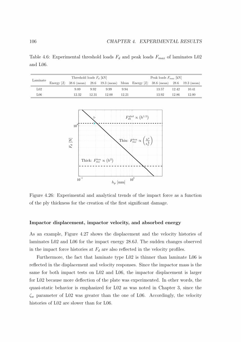
106 CHAPTER 4. EXPERIMENTAL RESULTS
Table 4.6: Experimental threshold loads Fd and peak loads Fmax of laminates L02
and L06.
LaminateThreshold loads Fd [kN] Peak loads Fmax [kN]
Energy [J]: 38.6 (mean) 28.6 19.3 (mean) Mean Energy [J]: 38.6 (mean) 28.6 19.3 (mean)
L02 9.89 9.92 9.99 9.94 13.57 12.42 10.41
L06 12.32 12.31 12.00 12.21 13.92 12.86 12.00
10−1
100
104
F statd1 ∝
(h1.5
)
Thin: F tenmc ∝
(h2
h12p
)
Thick: F tenmc ∝
(h2
)
hp [mm]
Fd
[N]
Figure 4.26: Experimental and analytical trends of the impact force as a function
of the ply thickness for the creation of the first significant damage.
Impactor displacement, impactor velocity, and absorbed energy
As an example, Figure 4.27 shows the displacement and the velocity histories of
laminates L02 and L06 for the impact energy 28.6J. The sudden changes observed
in the impact force histories at Fd are also reflected in the velocity profiles.
Furthermore, the fact that laminate type L02 is thinner than laminate L06 is
reflected in the displacement and velocity responses. Since the impactor mass is the
same for both impact tests on L02 and L06, the impactor displacement is larger
for L02 because more deflection of the plate was experimented. In other words, the
quasi-static behavior is emphasized for L02 as was noted in Chapter 3, since the
ζw parameter of L02 was greater than the one of L06. Accordingly, the velocity
histories of L02 are slower than for L06.
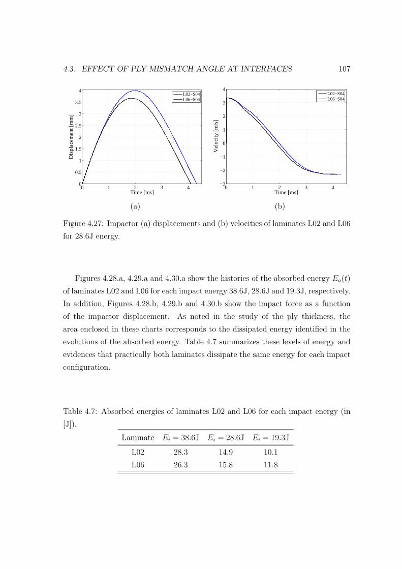
4.3. EFFECT OF PLY MISMATCH ANGLE AT INTERFACES 107
0 1 2 3 40
0.5
1
1.5
2
2.5
3
3.5
4
Time [ms]
Dis
plac
emen
t [m
m]
L02−S04L06−S04
0 1 2 3 4−3
−2
−1
0
1
2
3
4
Time [ms]
Vel
ocity
[m/s
]
L02−S04L06−S04
(a) (b)
Figure 4.27: Impactor (a) displacements and (b) velocities of laminates L02 and L06
for 28.6J energy.
Figures 4.28.a, 4.29.a and 4.30.a show the histories of the absorbed energy Ea(t)
of laminates L02 and L06 for each impact energy 38.6J, 28.6J and 19.3J, respectively.
In addition, Figures 4.28.b, 4.29.b and 4.30.b show the impact force as a function
of the impactor displacement. As noted in the study of the ply thickness, the
area enclosed in these charts corresponds to the dissipated energy identified in the
evolutions of the absorbed energy. Table 4.7 summarizes these levels of energy and
evidences that practically both laminates dissipate the same energy for each impact
configuration.
Table 4.7: Absorbed energies of laminates L02 and L06 for each impact energy (in
[J]).
Laminate Ei = 38.6J Ei = 28.6J Ei = 19.3J
L02 28.3 14.9 10.1
L06 26.3 15.8 11.8

108 CHAPTER 4. EXPERIMENTAL RESULTS
0 1 2 3 4 5 60
5
10
15
20
25
30
35
40
Time [ms]
Ene
rgy
[J]
L02−S01/S02/S03 (mean)L06−S01/S02/S03 (mean)
0 1 2 3 4 50
2000
4000
6000
8000
10000
12000
14000
Fd
Fd
Displacement [mm]F
orce
[N]
L02−S01/S02/S03 (mean)L06−S01/S02/S03 (mean)
(a) (b)
Figure 4.28: Evolution of the (a) absorbed energy and the (b) impact force versus
impactor displacement of laminates L02 and L06 for 38.6J.
0 1 2 3 40
5
10
15
20
25
30
Time [ms]
Ene
rgy
[J]
L02−S04L06−S04
0 1 2 3 40
2000
4000
6000
8000
10000
12000
14000
Fd
Fd
Displacement [mm]
For
ce [N
]
L02−S04L06−S04
(a) (b)
Figure 4.29: Evolution of the (a) absorbed energy and the (b) impact force versus
impactor displacement of laminates L02 and L06 for 28.6J.
4.3.2 NDI: C-scan after impact
Figure 4.31 shows a sample of C-scan inspections of laminates L02 and L06 for each
impact energy. The projected delamination areas of L06 are among square and
circular shaped. Although the C-scan inspections give the resulting damaged areas
after impact tests, these results can be associated with the analytical predictions

4.3. EFFECT OF PLY MISMATCH ANGLE AT INTERFACES 109
0 1 2 3 40
5
10
15
20
Time [ms]
Ene
rgy
[J]
L02−S05/S06 (mean)L06−S05/S06 (mean)
0 0.5 1 1.5 2 2.5 3 3.50
2000
4000
6000
8000
10000
12000
14000
Fd
Fd
Displacement [mm]
For
ce [N
]
L02−S05/S06 (mean)L06−S05/S06 (mean)
(a) (b)
Figure 4.30: Evolution of the (a) absorbed energy and the (b) impact force versus
impactor displacement of laminates L02 and L06 for 19.3J.
for the first significant damage Fd. As was noted in the discussion of the impact
force histories, Fd can be triggered by a circular mid-plane delamination. In an
approximate point of view, this argument suits with the resulted inspections.
According to the results of the ply thickness study, increasing the impact velocity
increases the projected delamination area for all laminates.
Ei = 38.6J Ei = 28.6J Ei = 19.3J
Figure 4.31: Sample of C-scan inspections of laminates L02 and L06.
Looking the results presented, the mismatch angle of the interfaces has not a

110 CHAPTER 4. EXPERIMENTAL RESULTS
clear effect on the damage resistance of the plate, despite the fact that laminate
L06 was selected because its stacking sequence has increased mismatch angles in
comparison with laminate L02. This lack of contrast may be generated by the
differences in the plate thicknesses of L02 and L06 which make difficult to extract
a possible concluding result, or simply because really the mismatch angle does not
affect the damage resistance significantly.
4.3.3 Dent-depth measurements
In Figure 4.32 are collected the contour plots of the dent-depth measurements of
the whole selected specimen sample of laminates L02 and L06. The shape of the
contour plots for L06 are circular in the center and changes into a square shape as
more far from the impact point the lecture is. As can be observed, increasing the
impact velocity, the resulting indentation obviously is increased. On the other hand,
an effect of the mismatch angle is not detected.
Ei = 38.6J Ei = 28.6J Ei = 19.3J
Length [mm]
Wid
th [m
m]
L02−S02Maximum indentation: 0.837 mm
50 60 70 80 90 10030
35
40
45
50
55
60
65
70
0
0.2
0.4
0.6
0.8
1
Length [mm]
Wid
th [m
m]
L02−S04Maximum indentation: 0.213 mm
50 60 70 80 90 10030
35
40
45
50
55
60
65
70
0
0.2
0.4
0.6
0.8
1
Length [mm]
Wid
th [m
m]
L02−S05Maximum indentation: 0.206 mm
50 60 70 80 90 10030
35
40
45
50
55
60
65
70
0
0.2
0.4
0.6
0.8
1
Length [mm]
Wid
th [m
m]
L06−S03Maximum indentation: 0.338 mm
50 60 70 80 90 10030
35
40
45
50
55
60
65
70
0
0.1
0.2
0.3
0.4
0.5
0.6
0.7
0.8
Length [mm]
Wid
th [m
m]
L06−S04Maximum indentation: 0.293 mm
50 60 70 80 90 10030
35
40
45
50
55
60
65
70
0
0.1
0.2
0.3
0.4
0.5
0.6
0.7
0.8
Length [mm]
Wid
th [m
m]
L06−S06Maximum indentation: 0.228 mm
50 60 70 80 90 10030
35
40
45
50
55
60
65
70
0
0.1
0.2
0.3
0.4
0.5
0.6
0.7
0.8
Figure 4.32: Dent-depth inspections of laminates L02 and L06.

4.3. EFFECT OF PLY MISMATCH ANGLE AT INTERFACES 111
4.3.4 CAI tests
Residual compressive load
Table 4.8 summarizes the residual compressive loads Ffc obtained. As it can be
evidenced, increasing the impact energy (or the impact velocity), the residual com-
pressive loads are reduced for any laminate.
Table 4.8: Failure compressive loads Ffc of laminates L02 and L06.
Ei = 38.6J Ei = 28.6J Ei = 19.3J
Specimen Ffc [kN] Specimen Ffc [kN] Specimen Ffc [kN]
L02-S01 93 L02-S04 103 L02-S05 133
L02-S02 99
Mean: 96
L06-S01 113 L06-S04 130 L06-S06 145
L06-S02 114
Mean: 114
In addition, the compressive loads of L06 are larger than for L02. This result can
not be attributed to the effect of the ply mismatch angle, and even more when it is
expected that the mismatch angle should give a reduced damage tolerance as noted
in Chapter 3. Really, the residual loads of L06 are larger because laminate L06 has
more plies than L02. Therefore, if these loads are normalized by the corresponding
section subjected in compression (i.e. b × h), the compressive residual strengths
obtained for both laminates are practically equal at each impact energy (see Table
4.9).
Table 4.9: Residual compressive strengths σfc of laminates L02 and L06.
LaminateEi = 38.6J Ei = 28.6J Ei = 19.3J
Ffc [kN] σfc [MPa] Ffc [kN] σfc [MPa] Ffc [kN] σfc [MPa]
L02 96 16.6 103 17.8 133 22.9
L06 114 16.8 130 19.1 145 21.3

112 CHAPTER 4. EXPERIMENTAL RESULTS
Lectures of the displacement transducers (LVDT) and the strain gages
(SG)
Table 4.10 summarizes the maximum values of the lectures of the two displacement
transducers used during the CAI tests. As it can be observed, the values obtained are
quite similar for both laminate types. In addition, Figure 4.33 shows the lectures
for laminates L02 and L06 of the specimens impacted with 29.6J. As in the ply
clustering study, the buckling mode of each laminate type is practically the same.
Table 4.10: Maximum lectures of the displacement transducers of laminates L02 and
L06.
Impact energy: Ei = 38.6J Impact energy: Ei = 28.6J Impact energy: Ei = 19.3J
Specimen LVDT1 [mm] LVDT2 [mm] Specimen LVDT1 [mm] LVDT2 [mm] Specimen LVDT1 [mm] LVDT2 [mm]
L02-S01 1.67 0.09 L02-S04 1.73 0.16 L02-S05 1.11 0.41
L02-S02 2.06 0.33
L06-S01 2.08 0.30 L06-S04 1.55 0.37 L06-S06 1.50 0.22
L06-S02 2.22 0.26
−1.5 −1 −0.5 00
2
4
6
8
10
12x 10
4
Displacement [mm]
For
ce [N
]
L02−S04 (LVDT1)L02−S04 (LVDT2)
−1.5 −1 −0.5 00
2
4
6
8
10
12
14x 10
4
Displacement [mm]
For
ce [N
]
L06−S04 (LVDT1)L06−S04 (LVDT2)
(a) (b)
Figure 4.33: Displacement transducer lectures of the specimens impacted with 29.6J:
(a) L02 and (b) L06.
Finally, Figure 4.34 shows the lectures of the four strain gages of each laminate
type for the impact energy of 29.6J. Again, differences between the lectures of the
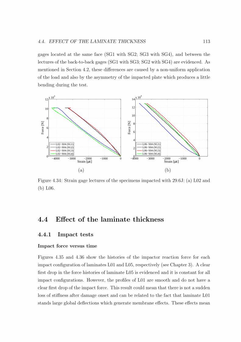
4.4. EFFECT OF THE LAMINATE THICKNESS 113
gages located at the same face (SG1 with SG2; SG3 with SG4), and between the
lectures of the back-to-back gages (SG1 with SG3; SG2 with SG4) are evidenced. As
mentioned in Section 4.2, these differences are caused by a non-uniform application
of the load and also by the asymmetry of the impacted plate which produces a little
bending during the test.
−4000 −3000 −2000 −1000 00
2
4
6
8
10
12x 10
4
Strain [µε]
For
ce [N
]
L02−S04 (SG1)L02−S04 (SG2)L02−S04 (SG3)L02−S04 (SG4)
−4000 −3000 −2000 −1000 00
2
4
6
8
10
12
14x 10
4
Strain [µε]
For
ce [N
]
L06−S04 (SG1)L06−S04 (SG2)L06−S04 (SG3)L06−S04 (SG4)
(a) (b)
Figure 4.34: Strain gage lectures of the specimens impacted with 29.6J: (a) L02 and
(b) L06.
4.4 Effect of the laminate thickness
4.4.1 Impact tests
Impact force versus time
Figures 4.35 and 4.36 show the histories of the impactor reaction force for each
impact configuration of laminates L01 and L05, respectively (see Chapter 3). A clear
first drop in the force histories of laminate L05 is evidenced and it is constant for all
impact configurations. However, the profiles of L01 are smooth and do not have a
clear first drop of the impact force. This result could mean that there is not a sudden
loss of stiffness after damage onset and can be related to the fact that laminate L01
stands large global deflections which generate membrane effects. These effects mean
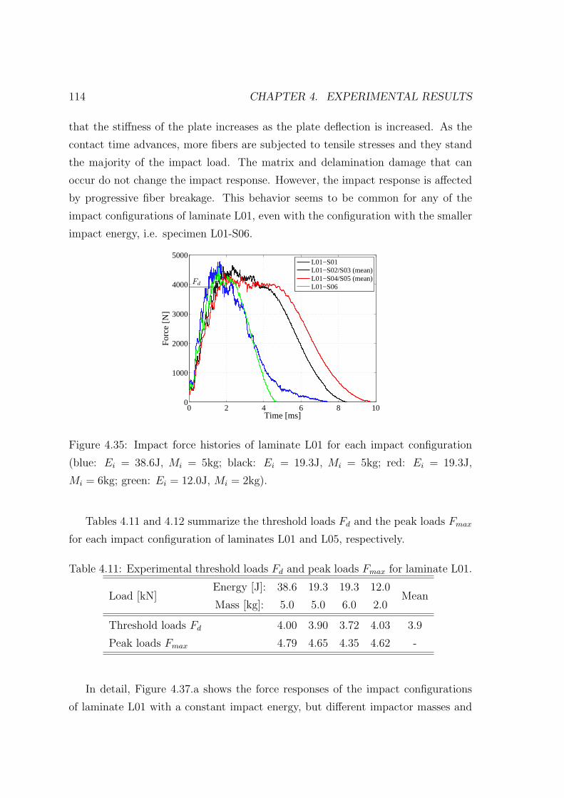
114 CHAPTER 4. EXPERIMENTAL RESULTS
that the stiffness of the plate increases as the plate deflection is increased. As the
contact time advances, more fibers are subjected to tensile stresses and they stand
the majority of the impact load. The matrix and delamination damage that can
occur do not change the impact response. However, the impact response is affected
by progressive fiber breakage. This behavior seems to be common for any of the
impact configurations of laminate L01, even with the configuration with the smaller
impact energy, i.e. specimen L01-S06.
0 2 4 6 8 100
1000
2000
3000
4000
5000
Fd
Time [ms]
For
ce [N
]
L01−S01L01−S02/S03 (mean)L01−S04/S05 (mean)L01−S06
Figure 4.35: Impact force histories of laminate L01 for each impact configuration
(blue: Ei = 38.6J, Mi = 5kg; black: Ei = 19.3J, Mi = 5kg; red: Ei = 19.3J,
Mi = 6kg; green: Ei = 12.0J, Mi = 2kg).
Tables 4.11 and 4.12 summarize the threshold loads Fd and the peak loads Fmax
for each impact configuration of laminates L01 and L05, respectively.
Table 4.11: Experimental threshold loads Fd and peak loads Fmax for laminate L01.
Load [kN]Energy [J]: 38.6 19.3 19.3 12.0
MeanMass [kg]: 5.0 5.0 6.0 2.0
Threshold loads Fd 4.00 3.90 3.72 4.03 3.9
Peak loads Fmax 4.79 4.65 4.35 4.62 -
In detail, Figure 4.37.a shows the force responses of the impact configurations
of laminate L01 with a constant impact energy, but different impactor masses and

4.4. EFFECT OF THE LAMINATE THICKNESS 115
0 1 2 3 4 5 60
0.5
1
1.5
2
x 104
Fd
Time [ms]
For
ce [N
]
L05−S01/S02 (mean)L05−S03/S04 (mean)L05−S05/S06 (mean)
Figure 4.36: Impact force histories of laminate L05 for each impact configuration
(blue: Ei = 38.6J, Mi = 5kg; black: Ei = 57.8J, Mi = 6kg; red: 57.9J, Mi = 15kg).
Table 4.12: Experimental threshold loads Fd and peak loads Fmax for laminate L05.
Load [kN]Energy [J]: 38.6 57.8 57.9
MeanMass [kg]: 5.0 6.0 15.0
Threshold loads Fd 18.84 19.59 19.56 19.33
Peak loads Fmax 18.84 19.77 19.95 -
velocities. As can be observed, increasing the impactor mass the response is more
quasi-static, which means that the response is slowed down. In addition, Figure
4.37.b also shows the same analysis for laminate L05, but in this case the difference
in the impactor mass is increased, yielding to more differentiable responses.
The effect of the impactor mass Mi was shown in the impact characterization
diagram by means of the relative mobility parameter ζw (see Chapter 2). Increasing
Mi, ζw is increased and then the behavior is changed to a more quasi-static behavior.
This effect can also be observed by means of the complete analytical models of the
impact event. Accordingly, Figure 4.38 show the experimental and the analytical
responses of laminate L01 for the impact energy 19.3J. In detail, the analytical
predictions plotted in Figure 4.38.a are given by a complete model fed with the bi-

116 CHAPTER 4. EXPERIMENTAL RESULTS
0 2 4 6 8 100
1000
2000
3000
4000
5000
Time [ms]
For
ce [N
]
L01−S02/S03 (mean)L01−S04/S05 (mean)
0 1 2 3 4 5 60
0.5
1
1.5
2
x 104
Time [ms]F
orce
[N]
L05−S03/S04 (mean)L05−S05/S06 (mean)
(a) (b)
Figure 4.37: (a) Impact force histories of laminate L01 for 19.3J (black: Mi = 5kg;
red: Mi = 6kg), and (b) impact force histories of laminate L05 for 58J (black:
Mi = 6kg; red: Mi = 15kg).
linear elastic-plastic contact law proposed by Yigit and Christoforou [45]. However,
for the model used for the predictions plotted in Figure 4.38.b, the Hertz contact law
is considered. For all the simulations, the number of modes applied for the Navier
solution is 5 for each in-plane x and y directions. The analytical models show
clearly the effect of changing the mass and the velocity under equal impact energy.
As expected, the contact time of the elastic responses is enlarged when the impactor
mass is increased. Finally, related to the contact laws used for the analytical models,
both cases suit the experimental profile and then no significant dependence with the
contact law is detected. This result is explained with the fact that laminate L01 has
small peak loads and an emphasized global behavior. Therefore, the role that plays
the contact law in these impact configurations is small.
Additionally, Figure 4.39 illustrates also the effect of changing the impactor
mass for laminate L05. In contrast with the predictions given for laminate L01, the
role that plays the contact law is significant because a more localized behavior is
experimented. As can be observed, the model which uses the Hertz contact law (in
Figure 4.39.b), suits better the experimental results than the model fed with the bi-
linear elastic-plastic contact law (in Figure 4.39.a). Therefore, given the predictions
of the complete models, it could be interesting to carry out quasi-static indentation

4.4. EFFECT OF THE LAMINATE THICKNESS 117
tests or finite element simulations in order to know what is the proper contact law.
Finally, the effects of changing the impactor mass and the velocity but keeping
constant the impact energy on the damage creation, can be simply analyzed, in a
qualitative point of view, by observing the peak loads of the analytical profiles or
by calculating the maximum elastic impact force as: Fmax = Fmax√ky√
2Ei (see
Section 3.2). Since the impact energy Ei is kept constant, it yields to a constant
maximum elastic impact force. Therefore, the resulting extension and type of dam-
age is expected to be the same.
0 2 4 6 8 100
1000
2000
3000
4000
5000
6000
7000
8000
Time [ms]
Forc
e [N
]
Experimental: Ei = 19.3J, Mi = 5.0kgExperimental: Ei = 19.3J, Mi = 6.0kgAnalytical: Ei = 19.3J, Mi = 5.0kgAnalytical: Ei = 19.3J, Mi = 6.0kg
0 2 4 6 8 100
1000
2000
3000
4000
5000
6000
7000
8000
Time [ms]
Forc
e [N
]
Experimental: Ei = 19.3J, Mi = 5.0kgExperimental: Ei = 19.3J, Mi = 6.0kgAnalytical: Ei = 19.3J, Mi = 5.0kgAnalytical: Ei = 19.3J, Mi = 6.0kg
(a) (b)
Figure 4.38: Experimental and analytical impact force histories of laminate L01
for a constant impact energy 19.3J: Mi = 5kg (black), and Mi = 6kg (red). Two
different contact laws are used: (a) bi-linear elastic-plastic contact law [45], and (b)
the Hertz contact law.
In Figure 4.40.a, the impact force histories corresponding to laminates L01 and
L02 for an impact energy of 19.3J and an impactor mass of 5kg are compared.
The effect of the plate thickness is clearly evidenced. Increasing the thickness, the
response is faster, the peak load increases, and a clear first drop of the force appears.
In addition, in Figure 4.40.b the impact force histories corresponding to laminates
L01, L02 and L05 for an impact energy of 38.6J and an impactor mass of 5kg are
compared. Again, the effects of the plate thickness under equal impact conditions
can be observed. As shown, laminate L01 was perforated under an impact with a
quasi-static behavior, as predicted in Chapter 3.
Recovering the experimental damage thresholds Fd of all laminates with equal

118 CHAPTER 4. EXPERIMENTAL RESULTS
0 1 2 3 4 5 60
0.5
1
1.5
2
2.5
3x 10
4
Time [ms]
Forc
e [N
]
Exp.: Ei = 57.8J, Mi = 6.0kgExp.: Ei = 57.9J, Mi = 15.0kgAn.: Ei = 57.8J, Mi = 6.0kgAn.: Ei = 57.9J, Mi = 15.0kg
0 1 2 3 4 5 60
1
2
3
4
5x 10
4
Time [ms]Fo
rce
[N]
Exp.: Ei = 57.8J, Mi = 6.0kgExp.: Ei = 57.9J, Mi = 15.0kgAn.: Ei = 57.8J, Mi = 6.0kgAn.: Ei = 57.9J, Mi = 15.0kg
(a) (b)
Figure 4.39: Experimental and analytical impact force histories of laminate L05 for
a constant impact energy 57.8J: Mi = 6kg (black), and Mi = 15kg (red). Two
different contact laws are used: (a) bi-linear elastic-plastic contact law [45], and (b)
the Hertz contact law.
0 2 4 6 80
2000
4000
6000
8000
10000
12000
Time [ms]
For
ce [N
]
L01−S02/S03 (mean)L02−S05/S06 (mean)
0 2 4 6 80
0.5
1
1.5
2x 10
4
Time [ms]
For
ce [N
]
L01−S01L02−S01/S02/S03 (mean)L05−S01/S02 (mean)
Perforation
(a) (b)
Figure 4.40: (a) Impact force histories of laminates L01 (black) and L02 (blue) for
19.3J; (b) impact force histories of laminates L01 (black), L02 (blue) and L05 (red),
for 38.6J.
ply thickness (L01, L02, L05 and L06), these can be plotted as a function of the
plate thickness h in a natural logarithmic scale, as shown in Figure 4.41. If a fit

4.4. EFFECT OF THE LAMINATE THICKNESS 119
of the experimental points is performed (in gray), a slope of 1.47 is obtained. This
value is quite close to the slope of the analytical threshold for a circular mid-plane
delamination (in black), i.e. 1.5, since F statd1 ∝ h1.5. Despite the constant offset that
exists between the experimental and the analytical values, the significant conclusion
is that the analytical trend seems to be in agreement with the experimental results.
This result suggests that these laminates have a threshold load that corresponds
approximately to a circular mid-plane delamination. The offset can be due to scat-
tering of the material properties or to the assumptions considered in the formulation
of the damage threshold, e.g. strain rate effects are neglected. Additionally, this
result agrees with the analytical prediction for the first significant damage explained
in Section 3.2.2, in exception of laminate L01. The damage threshold for L01 was
related to a back face delamination (Fd = F tenmc ). This inaccurate prediction can be
attributed to the fact that the identification of Fd in the impact force history is not
clear, or simply a sudden delamination does not occur.
101
104
h [mm]
Fd
[N]
L01
L02
L05L06
Experimental
AnalyticalF stat
d1 ∝(h1.5
)
Figure 4.41: Experimental and analytical threshold loads as a function of the plate
thickness.
Impactor displacement, impactor velocity, and absorbed energy
Accordingly to the impact force histories, the effect of changing the impactor mass
and the velocity, but keeping constant the impact energy, can also be observed in

120 CHAPTER 4. EXPERIMENTAL RESULTS
the histories of the impactor displacement and velocity plotted in Figure 4.42 for
laminate L01, and in Figure 4.43 for laminate L05. Increasing the impactor mass,
the displacements are enlarged and so the velocity responses are slower.
0 2 4 6 8 10 120
1
2
3
4
5
6
7
Time [ms]
Dis
plac
emen
t [m
m]
L01−S02/S03 (mean)L01−S04/S05 (mean)
0 2 4 6 8 10 12−2
−1
0
1
2
3
Time [ms]
Vel
ocity
[m/s
]
L01−S02/S03 (mean)L01−S04/S05 (mean)
(a) (b)
Figure 4.42: Impactor (a) displacement and (b) velocity of laminate L01 for 19.3J
(black: Mi = 5kg; red: Mi = 6kg).
0 1 2 3 4 5 6 70
1
2
3
4
5
Time [ms]
Dis
plac
emen
t [m
m]
L05−S03/S04 (mean)L05−S05/S06 (mean)
0 1 2 3 4 5 6 7−3
−2
−1
0
1
2
3
4
5
Time [ms]
Vel
ocity
[m/s
]
L05−S03/S04 (mean)L05−S05/S06 (mean)
(a) (b)
Figure 4.43: Impactor (a) displacement and (b) velocity of laminate L05 for 58J
(black: Mi = 6kg; red: Mi = 15kg).
Moreover, Figure 4.44.a shows the histories of the absorbed energy of laminates
L01, and Figure 4.44.b shows the evolutions of the impact force as a function of the
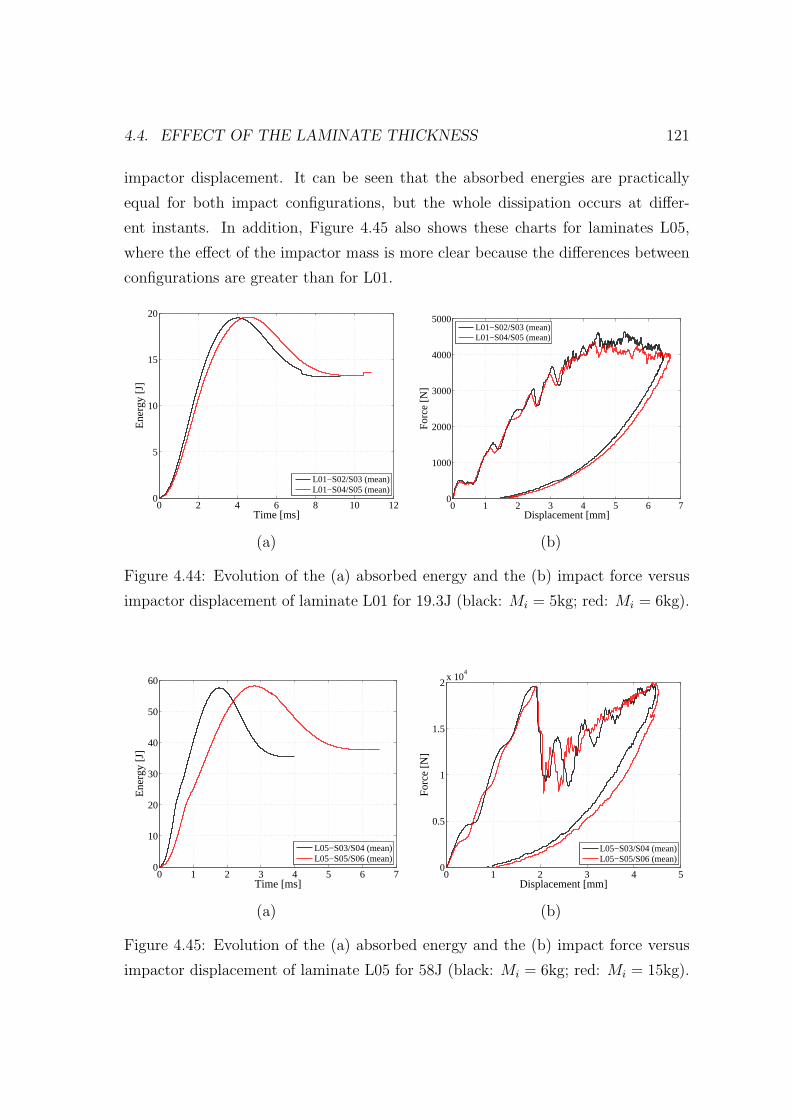
4.4. EFFECT OF THE LAMINATE THICKNESS 121
impactor displacement. It can be seen that the absorbed energies are practically
equal for both impact configurations, but the whole dissipation occurs at differ-
ent instants. In addition, Figure 4.45 also shows these charts for laminates L05,
where the effect of the impactor mass is more clear because the differences between
configurations are greater than for L01.
0 2 4 6 8 10 120
5
10
15
20
Time [ms]
Ene
rgy
[J]
L01−S02/S03 (mean)L01−S04/S05 (mean)
0 1 2 3 4 5 6 70
1000
2000
3000
4000
5000
Displacement [mm]
For
ce [N
]
L01−S02/S03 (mean)L01−S04/S05 (mean)
(a) (b)
Figure 4.44: Evolution of the (a) absorbed energy and the (b) impact force versus
impactor displacement of laminate L01 for 19.3J (black: Mi = 5kg; red: Mi = 6kg).
0 1 2 3 4 5 6 70
10
20
30
40
50
60
Time [ms]
Ene
rgy
[J]
L05−S03/S04 (mean)L05−S05/S06 (mean)
0 1 2 3 4 50
0.5
1
1.5
2x 10
4
Displacement [mm]
For
ce [N
]
L05−S03/S04 (mean)L05−S05/S06 (mean)
(a) (b)
Figure 4.45: Evolution of the (a) absorbed energy and the (b) impact force versus
impactor displacement of laminate L05 for 58J (black: Mi = 6kg; red: Mi = 15kg).

122 CHAPTER 4. EXPERIMENTAL RESULTS
The result detected in Figures 4.44 and 4.45 agrees with the procedure of the
guidelines for a drop-weight impact test provided by the aeronautical industry, which
often do not specify the impactor mass or the velocity, rather they establish the
impact energy (e.g. Airbus AITM1-0010 [94]). The reason for defining the set-up in
this way is related to the fact that independently of the impactor mass and velocity
selected, at the end of the test the energy dissipated will be the same. In other
words, the damage developed in the specimens is the same if the impact energy is
kept constant.
On the other hand, Figure 4.46 shows the displacement and the velocity histories
of laminates L01 and L02 for the impact energy 19.3J. In addition, Figure 4.47
shows the corresponding histories of laminates L01, L02 and L05 for the impact
energy 38.6J. Again, the effect of the laminate thickness is evidenced. Increasing
the thickness, the response is more localized. This result means that the impactor
displacement is smaller because less global deflection of the plate is experienced, and
accordingly the response is much faster.
0 2 4 6 8 100
1
2
3
4
5
6
7
Time [ms]
Dis
plac
emen
t [m
m]
L01−S02/S03 (mean)L02−S05/S06 (mean)
0 2 4 6 8 10−2
−1
0
1
2
3
Time [ms]
Vel
ocity
[m/s
]
L01−S02/S03 (mean)L02−S05/S06 (mean)
(a) (b)
Figure 4.46: Impactor (a) displacement and (b) velocity of laminates L01 and L02
for 19.3J.
The absorbed energy is not the same for each laminate thickness under equal
impact conditions. The trend is if the laminate thickness is increased, the absorbed
energy is reduced. This effect can be observed in Figure 4.48, which shows the
histories of the absorbed energy and the evolutions of the impact force as a function

4.4. EFFECT OF THE LAMINATE THICKNESS 123
0 2 4 6 80
2
4
6
8
10
12
14
16
18
Time [ms]
Dis
plac
emen
t [m
m]
L01−S01L02−S01/S02/S03 (mean)L05−S01/S02 (mean)
Perforation
0 2 4 6 8−3
−2
−1
0
1
2
3
4
Time [ms]
Vel
ocity
[m/s
]
L01−S01L02−S01/S02/S03 (mean)L05−S01/S02 (mean)
Perforation
(a) (b)
Figure 4.47: Impactor (a) displacement and (b) velocity of laminates L01, L02 and
L05 for 38.6J.
of the impactor displacement of laminates L01 and L02 for the impact energy 19.3J.
The dissipated energies at the end of the tests are 13.1J for L01 and 10.1J for L02.
Additionally, Figure 4.49 shows these evolutions corresponding to laminates L01,
L02 and L05 for the impact energy 38.6J. In this case, the dissipated energies at
the end of the tests are 34.3J for L01, 28.3J for L02, and 23.6J for L05. Finally, a
recovering of the elastic energy in the evolution of Ea of the perforated specimen
L01-S06 is not observed.
4.4.2 NDI: C-scan after impact
The observations commented before about the effects of changing the impactor mass
and the velocity, but keeping constant the impact energy, also can be associated
with the ultrasonic C-scan inspections. Figures 4.50 and 4.51 show a sample of
the projected delamination areas corresponding to laminate L01 and laminate L05,
respectively. It is observed that the projected area is practically the same when the
impact energy is kept constant. This result suits with the fact that the dissipated
energy is also the same for two impact cases which have the same impact energy.
On the other hand, between specimens with the same impact configuration but
different laminate thicknesses, the resulting values of the projected area are quite
similar, such as it is shown in Figures 4.52 and 4.53. However, it could be interesting

124 CHAPTER 4. EXPERIMENTAL RESULTS
0 2 4 6 8 100
5
10
15
20
Time [ms]
Ene
rgy
[J]
L01−S02/S03 (mean)L02−S05/S06 (mean)
0 1 2 3 4 5 6 70
2000
4000
6000
8000
10000
12000
Displacement [mm]
For
ce [N
]
L01−S02/S03 (mean)L02−S05/S06 (mean)
(a) (b)
Figure 4.48: Evolution of the (a) absorbed energy and the (b) impact force versus
impactor displacement of laminates L01 and L02 for 19.3J.
0 2 4 6 80
5
10
15
20
25
30
35
40
Time [ms]
Ene
rgy
[J]
L01−S01L02−S01/S02/S03 (mean)L05−S01/S02 (mean)
Perforation
0 5 10 150
0.5
1
1.5
2x 10
4
Displacement [mm]
For
ce [N
]
L01−S01L02−S01/S02/S03 (mean)L05−S01/S02 (mean)
(a) (b)
Figure 4.49: Evolution of the (a) absorbed energy and the (b) impact force versus
impactor displacement of laminates L01, L02 and L05 for 38.6J.
to have at one’s disposal the total values of the sum of each delaminated area of
the interfaces, and then to compare these values between laminates with different
thicknesses. Therefore, it could be expected that the largest area would be from
laminate L01 as it was detected in the profiles of the dissipated energy. If this
does not occur, then other damage mechanisms should have absorbed the energy in

4.4. EFFECT OF THE LAMINATE THICKNESS 125
Ei = 19.3J; Mi = 5.0kg Ei = 19.3J; Mi = 6.0kg
Figure 4.50: Sample of C-scan inspections of laminate L01 with equal impact ener-
gies, but different impactor masses.
Ei = 57.8J; Mi = 6.0kg Ei = 57.9J; Mi = 15.0kg
Figure 4.51: Sample of C-scan inspections of laminate L05 with equal impact ener-
gies, but different impactor masses.
laminate L01, such as fiber breakage.
L01 L02
Figure 4.52: Sample of C-scan inspections of laminates L01 and L02 for 19.3J (lam-
inate thickness).
The shapes of the projected delamination areas can be related to the analytical
predictions of Fd. For laminate type L01 was predicted a delamination at the first
interface from the back face of the plate (i.e. F tenmc for thin ply thickness). How-
ever, the experimental value obtained fits with the global linear trend for a circular

126 CHAPTER 4. EXPERIMENTAL RESULTS
L01 L02 L05
Figure 4.53: Sample of C-scan inspections of laminates L02 and L05 for 38.6J (lam-
inate thickness).
mid-plane delamination F statd1 , as it was seen in Figure 4.41. Figure 4.54 shows the
ultrasonic inspection for the laminate L01 with the lowest impact energy. As can
be observed, the shape is equal in comparison with the shapes resulted from higher
impact energies, just that with a smaller size. Therefore, for laminate L01 it is dif-
ficult to know what is the damage type associated to Fd. As was noted previously,
these difficulties can be due to different factors. On the other hand, the prediction
of Fd for both laminate types L02 and L05 was a mid-plane circular delamination.
The shapes obtained are quite circular, but it should be noted that these circu-
lar shapes are rather a result of the superposition of peanut shaped delaminations.
Furthermore, the deeper the delamination is, the larger the delamination is. These
distribution of delaminations yield to the so-called pine pattern delamination dis-
tribution. In conclusion, for laminates L02 and L05 the prediction of Fd can be
considered well suited although the considerations commented.
Figure 4.54: C-scan inspection of specimen L01-S06 (Ei = 12.0J, Mi = 2.0kg).

4.4. EFFECT OF THE LAMINATE THICKNESS 127
4.4.3 Dent-depth measurements
Figures 4.55 and 4.56 show the contour plots of the dent depth measurements of
the impacted specimens L01 and L05, respectively. Consistent with previous obser-
vations, the resulting lectures of the dent depths are quite similar for impact cases
with different impactor mass and velocity, but with equal impact energy.
Ei = 19.3J; Mi = 5.0kg Ei = 19.3J; Mi = 6.0kg
Length [mm]
Wid
th [m
m]
L01−S02Maximum indentation: 0.987 mm
50 60 70 80 90 10030
35
40
45
50
55
60
65
70
0
0.2
0.4
0.6
0.8
1
Length [mm]
Wid
th [m
m]
L01−S04Maximum indentation: 1.164 mm
50 60 70 80 90 10030
35
40
45
50
55
60
65
70
0
0.2
0.4
0.6
0.8
1
Figure 4.55: Dent-depth inspections of laminate L01 with equal impact energies,
but different impactor masses.
Ei = 57.8J; Mi = 6.0kg Ei = 57.9J; Mi = 15.0kg
Length [mm]
Wid
th [m
m]
L05−S03Maximum indentation: 0.335 mm
50 60 70 80 90 10030
35
40
45
50
55
60
65
70
0
0.05
0.1
0.15
0.2
0.25
0.3
Length [mm]
Wid
th [m
m]
L05−S06Maximum indentation: 0.306 mm
50 60 70 80 90 10030
35
40
45
50
55
60
65
70
0
0.05
0.1
0.15
0.2
0.25
0.3
Figure 4.56: Dent-depth inspections of laminate L05 with equal impact energies,
but different impactor masses.
Figures 4.57 and 4.58 show a sample of dent-depth measurements of laminates
with different thicknesses. As it was observed in the histories of the impact force, in-
creasing the laminate thickness, the response results more localized because less lam-
inate deflection is experimented. Conversely, the dent-depth measurements demon-
strate that also the indentation values are higher for thin plates. Nevertheless, it

128 CHAPTER 4. EXPERIMENTAL RESULTS
should be noted that for thin plates the indentation measurements are affected by the
residual global deflection of the plate which increases the measurements obtained.
Length [mm]
Wid
th [m
m]
L01−S02Maximum indentation: 0.987 mm
50 60 70 80 90 10030
35
40
45
50
55
60
65
70
0
0.2
0.4
0.6
0.8
Length [mm]
Wid
th [m
m]
L02−S05Maximum indentation: 0.206 mm
50 60 70 80 90 10030
35
40
45
50
55
60
65
70
0
0.2
0.4
0.6
0.8
Figure 4.57: Dent-depth inspections of laminates L01 and L02 for 19.3J.
Length [mm]
Wid
th [m
m]
L02−S02Maximum indentation: 0.837 mm
50 60 70 80 90 10030
35
40
45
50
55
60
65
70
0
0.1
0.2
0.3
0.4
0.5
0.6
0.7
0.8
Length [mm]
Wid
th [m
m]
L05−S01Maximum indentation: 0.218 mm
50 60 70 80 90 10030
35
40
45
50
55
60
65
70
0
0.1
0.2
0.3
0.4
0.5
0.6
0.7
0.8
Figure 4.58: Dent-depth inspections of laminates L02 and L05 for 38.6J.
4.4.4 CAI tests
Residual compressive load
The results available from the CAI test to check the effects of changing the impactor
mass but keeping constant the impact energy are those from laminate L05. The
residual compressive loads Ffc are: 164.5kN for Ei = 57.8J and Mi = 6.0kg, and
156.9kN for Ei = 57.9J and Mi = 15.0kg. It can be concluded that the values
obtained are quite similar as can be expected after the discussion of the results
presented before.
Increasing the laminate thickness under equal impact conditions, the residual
compressive load increases. However, in order to compare properly these data, the
normalized loads σfc must be computed. The resulting values are summarized in

4.4. EFFECT OF THE LAMINATE THICKNESS 129
Table 4.13. It can be expected that the values should be similar for each impact
energy, however it is not completely true because the size and the number of interface
delaminations created in the impact tests are different in function of the laminate
thickness. Therefore, given the available data, a valid argument can not be deduced.
Table 4.13: Residual compressive strengths σfc of laminates L01, L02 and L06.
Ei = 19.3J Ei = 38.6J
L01 L02 L02 L05
σfc [MPa] 19.7 22.9 16.5 20.6
Lectures of the displacement transducers (LVDT) and the strain gages
(SG)
As an example of the displacement transducer and strain gage lectures, Figure 4.59
shows the results obtained for laminate L05. Despite the differences in the impactor
mass and velocity, the responses are quite similar.
Finally, in order to illustrate the differences obtained in the responses of the
transducer displacement and strain gages due to the differences in the laminate
thickness, Figures 4.60 and 4.61 show the results obtained. It is observed that
laminate types L01 and L02 suffer a clear global buckling on the instrumented plate
face. This behavior is not observed in Figure 4.61, where both laminates L02 and
L05 suffer a more localized buckling in the middle point of the specimen lengths.

130 CHAPTER 4. EXPERIMENTAL RESULTS
Ei = 57.8J; Mi = 6.0kg Ei = 57.9J; Mi = 15.0kg
−2 −1.5 −1 −0.5 00
2
4
6
8
10
12
14
16
18x 10
4
Displacement [mm]
For
ce [N
]
L05−S03 (LVDT1)L05−S03 (LVDT2)
−1.5 −1 −0.5 00
2
4
6
8
10
12
14
16x 10
4
Displacement [mm]
For
ce [N
]
L05−S05 (LVDT1)L05−S05 (LVDT2)
−4000 −3000 −2000 −1000 00
2
4
6
8
10
12
14
16
18x 10
4
Strain [µε]
For
ce [N
]
L05−S03 (SG1)L05−S03 (SG2)L05−S03 (SG3)L05−S03 (SG4)
−4000 −3000 −2000 −1000 00
2
4
6
8
10
12
14
16x 10
4
Strain [µε]
For
ce [N
]
L05−S05 (SG1)L05−S05 (SG2)L05−S05 (SG3)L05−S05 (SG4)
(a) (b)
Figure 4.59: (a) Displacement transducer and (b) strain gage lectures of laminate
L05.

4.4. EFFECT OF THE LAMINATE THICKNESS 131
L01 L02
−3 −2.5 −2 −1.5 −1 −0.5 0 0.50
1
2
3
4
5
6x 10
4
Displacement [mm]
For
ce [N
]
L01−S04 (LVDT1)L01−S04 (LVDT2)
−1.2 −1 −0.8 −0.6 −0.4 −0.2 0 0.20
2
4
6
8
10
12
14x 10
4
Displacement [mm]
For
ce [N
]
L02−S05 (LVDT1)L02−S05 (LVDT2)
−7000 −6000 −5000 −4000 −3000 −2000 −1000 00
1
2
3
4
5
6x 10
4
Strain [µε]
For
ce [N
]
L01−S04 (SG1)L01−S04 (SG2)L01−S04 (SG3)
−6000 −5000 −4000 −3000 −2000 −1000 00
2
4
6
8
10
12
14x 10
4
Strain [µε]
For
ce [N
]
L02−S05 (SG1)L02−S05 (SG2)L02−S05 (SG3)L02−S05 (SG4)
(a) (b)
Figure 4.60: (a) Displacement transducer and (b) strain gage lectures of laminates
L01 and L02 for 19.3J.

132 CHAPTER 4. EXPERIMENTAL RESULTS
L02 L05
−2.5 −2 −1.5 −1 −0.5 0 0.50
2
4
6
8
10x 10
4
Displacement [mm]
For
ce [N
]
L02−S02 (LVDT1)L02−S02 (LVDT2)
−1.5 −1 −0.5 00
0.5
1
1.5
2x 10
5
Displacement [mm]
For
ce [N
]
L05−S01 (LVDT1)L05−S01 (LVDT2)
−4000 −3000 −2000 −1000 00
2
4
6
8
10x 10
4
Strain [µε]
For
ce [N
]
L02−S02 (SG1)L02−S02 (SG2)L02−S02 (SG3)L02−S02 (SG4)
−5000 −4000 −3000 −2000 −1000 0 10000
0.5
1
1.5
2x 10
5
Strain [µε]
For
ce [N
]
L05−S01 (SG1)L05−S01 (SG2)L05−S01 (SG3)L05−S01 (SG4)
(a) (b)
Figure 4.61: (a) Displacement transducer and (b) strain gage lectures of laminates
L02 and L05 for 38.6J.

4.5. SUMMARY OF CONCLUSIONS 133
4.5 Summary of conclusions
The main conclusions from the previous discussions of the experimental results and
the analytical predictions are presented herein. These conclusions are valid for drop-
weight impact events (i.e. low-velocity impacts), and most of them reaffirm some of
the arguments explained in the design of the experiments of Chapter 3.
Effect of the impact velocity
• The threshold load, Fd, remains constant in front of changes of the impact
velocity.
• Increasing the impact velocity, the slope of the elastic regime is increased, as
predicted by means of the analytical impact models. Accordingly, the pre-
dicted maximum elastic impact force increases, indicating that more damage
is created.
• Increasing the impact velocity, the response is extended in time because the
plate develops more damage. Accordingly, the post-impact residual compres-
sive strength is reduced.
Effect of changing the impactor mass and the velocity
• The threshold load, Fd, remains constant in front of changes of the impactor
mass and velocity, but keeping constant the impact energy.
• Increasing the impactor mass, the response is more quasi-static, which means
that the response is slowed down. This behavior was also predicted by means
of the impact characterization diagram and the complete analytical impact
models.
• Given a stacking sequence, the dissipated energy or the damage developed is
the same between impacts with equal impact energy. In addition, the residual
compressive strength remains constant under the same impact energy level.
This result agrees with some of the guidelines provided by the aeronautical
industry for a drop-weight impact test, where the energy is specified, and the
impactor mass and the velocity can be selected freely by the engineer.

134 CHAPTER 4. EXPERIMENTAL RESULTS
Effect of ply thickness (clustering)
• If the ply clustering is increased, under equal impact conditions the values of
Fd and Fmax are reduced.
• Increasing the ply clustering, the changes in the stiffness during the impact are
more progressive and smooth when compared with laminates with thin plies.
This result implies difficulties in the detection of Fd for laminates with thick
plies.
• The response is elongated by increasing the ply clustering of the laminate. This
result indicates that more damage develops for laminates with thick plies. Ac-
cordingly, by reducing the number of interfaces available for delamination, the
resulting projected delamination area is increased. Therefore, ply clustering
results in a lower damage resistance of a composite structure.
• Increasing the ply clustering, the indentation is increased.
• The free growth of the delaminations can be affected by the finite in-plane
dimensions of the plates. In other words, the growth of the delaminations could
be braked by the clamping system. This effect occurs basically in laminates
with thick plies.
• The trend of the proposed analytical thresholds for delamination are in agree-
ment with the experimental points for all laminate types. However, the ana-
lytical values under-predict the real values. This offset can be due to scattering
of the material properties or to the assumptions considered in the formulation
of the damage threshold, e.g. strain rate effects are neglected. Further testing
is required to verify these arguments, especially with critical impact energies
which generate maximum impact forces similar to the damage threshold loads.
• The damage tolerance, quantified using the residual compressive load, is not
affected by increasing the ply thickness, because all presented laminate types
have shown similar values of compressive loads at each impact energy.

4.5. SUMMARY OF CONCLUSIONS 135
Effect of ply mismatch angle at interfaces
• The analytical prediction of Fd for the selected cross-ply laminate has been in
agreement with the experimental result, although an offset also has appeared.
• The mismatch angle of the interfaces for delamination has not presented a clear
effect on the damage resistance and on the damage tolerance. This result can
be due to the fact that the plate thicknesses of the selected laminates for this
study are slightly different.
Effect of the laminate thickness
• Increasing the laminate thickness, the response is faster and the drop in the
impact force from point Fd increases. For the thinner laminate tested, the
profiles of the impact force are smooth and do not present a clear first drop
on the impact force. This result could mean that a sudden loss of stiffness
from the point Fd does not occur, or the matrix and delamination damage
that appear do not change the response of the impact, rather it is affected by
progressive fiber breakage. This last argument can be related to the membrane
effects.
• The predictions of the threshold load Fd for the different laminates considered
have been in agreement except for the thinner laminate, i.e. L01. This result
can be attributed to different causes: the membrane effects, the possibility
that really the delaminations can not be detected in the force histories, or the
fact that simply a sudden large delamination does not occur and rather the
delaminations grow progressively.
• Increasing the laminate thickness, the damage resistance is improved since
the energy dissipated is lower than for thin laminates. Likewise, the damage
tolerance is improved. However, the resulting structures are heavier and more
expensive.
Usefulness of the analytical impact models and analytical thresholds
• With the studies presented, it has been demonstrated that the analytical im-
pact models for the prediction of the elastic response are a powerful tool: to

136 CHAPTER 4. EXPERIMENTAL RESULTS
define a suitable test matrix of specimens, to obtain a qualitative understand-
ing of the effects of the governing parameters on the impact response, and to
interpret the experimental results obtained.
• The analytical impact models are completed with the analytical thresholds for
the prediction of the damage mechanisms that can occur in a laminated com-
posite plate under low-velocity impact loading. For low-velocity impacts, the
most critical damage is the delamination. In general, it has been shown that
the damage thresholds for delamination follow the trends of the experimen-
tal results. Table 4.14 summarizes the analytical and experimental thresholds
obtained.
Table 4.14: Summary of analytical and experimental thresholds.
LaminateAnalytical Fd [kN]
Experimental Fd [kN] C-scan shapeF statd1 F ten
mc
L01 3.16 2.68 3.90
L02 8.53 10.34 9.94
L03 8.49 7.20 7.60
L04 8.34 4.92 5.50
L05 15.97 23.80 19.33
L06 10.65 11.26 12.21

Chapter 5
Interlaminar damage model
5.1 Introduction
Delamination is one of the most common failure mechanisms in laminated composite
materials and can appear at any life time of the structure (manufacturing, trans-
portation, assembly, and service). Delamination reduces seriously the integrity of a
structural element and can produce its collapse. Therefore, accurate analysis tools
for the simulation of delamination are required.
Delamination has been largely studied and modeled in the literature. When
material nonlinearities can be neglected and an initial crack is present, methods
based on Linear Elastic Fracture Mechanics (LEFM) have been proven to be effective
in predicting delamination growth, such as the Virtual Crack Closure Technique
(Irwin [100]; Rybicki and Kanninen [101]; Raju [102]; Zou et al. [103]; Krueger
[104]), the J-integral method (Rice [105]), the virtual crack extension (Hellen [106]),
and the stiffness derivative (Parks [107]). These techniques are used to calculate
the components of the energy release rate. Delamination growth is predicted when
a combination of the components of the energy release rate is equal to, or greater
than, a critical value (Griffith [108]).
When no initial macroscopic defects are present, a local approach has been fre-
quently used to detect delamination onset, in which the key parameters are critical
values of tractions (e.g. Pagano and Pipes [109], and Hashin [110]).
Another approach for delamination modeling can be developed within the frame-
work of Damage Mechanics. Models formulated using Damage Mechanics considers
137

138 CHAPTER 5. INTERLAMINAR DAMAGE MODEL
an interface as a third independent material defined by its own constitutive law.
This interface links the two structural components and is based on the concept of
the cohesive crack model introduced by Barenblatt [111], Dugdale [112], Hillerborg
et al. [113] and others: a cohesive damage zone or softening plasticity is developed
near the crack front. Cohesive damage zone models relate tractions to displacement
jumps at an interface where a crack may occur. Damage initiation is related to the
interfacial strength (i.e. the maximum traction on the traction-displacement jump
relation). When the area under the traction-displacement jump relation is equal
to the fracture toughness, the traction is reduced to zero and new crack surfaces
are formed. The use of cohesive models is extremely powerful for the simulation of
general fracture processes due to its simplicity and the unification of crack initiation
and growth within one model.
The implementation of cohesive constitutive models normally is carried out by
means of user-written subroutines in finite element codes. Generally, the examples
presented in the literature implement cohesive elements (e.g. Schellekens and De
Borst [114], Allix et al. [115], Mi et al. [116], Alfano and Crisfield [117], Camanho
et al. [118], and De Borst [119]) or a user material definition (e.g. Pinho et al. [120],
Iannucci [121], and Aymerich et al. [122]), although surface-based cohesive behaviors
which eliminate the need to define cohesive elements have been also implemented
(e.g. Zhang et al. [123], and Abaqus 6.8 [124]).
In cases where crack path is known in advance, either from experimental evi-
dence, or because of the material configuration, discrete interface elements equipped
with a cohesive constitutive relation are inserted a priori in the finite element mesh
(e.g. Corigliano and Allix [125]). To allow for a more arbitrary direction of crack
propagation, interface elements can be inserted between all continuum elements (Xu
and Needleman [126]). However, this approach is limited to a number of predefined
orientation crack angles since the interface elements are aligned with the element
boundaries. Some authors (e.g. Martha et al. [127], and De Borst [119]) use mesh-
ing tools to redefine the position of cohesive elements in function of the stress state
evolution. When the position for the appearance and progression of a crack is de-
tected, the structure is again meshed and an interface element is located in a proper
position. Alternatively, another research line in fracture modeling is to improve the
kinematic description of finite elements by enriching the shape functions by means

5.1. INTRODUCTION 139
of adding degrees of freedom. Initially, these models consider a law which relates
the stresses and the strains until damage localization is detected in one plane. At
this point, the law is rewritten and relates stresses and crack opening. Some of these
approaches are: elements with embedded discontinuities (e.g. Oliver [128]) based on
the enhanced assumed strain (Simo and Rifai [129]), and extended finite elements
(e.g. Belytschko et al. [130]) based on partition of unity method (Babuska and
Melenk [131]).
In the formulation of cohesive models, the energy dissipated during the crack
opening has to be controlled, i.e. it is necessary to assure that the model satisfies the
Clausius-Duhem inequality. Some models are well suited to simulate delamination
under constant mixed-mode conditions, such as Mi et al. [116], Alfano and Crisfield
[117]. However, these models do not satisfy the Clausius-Duhem inequality when
the crack grows in variable mixed-mode conditions, because generally they define
the damage threshold parameter as the maximum displacement and the damage
variable as a function of material parameters that depend on the mixed-mode ratio.
Examples of cohesive models which develop in a thermodynamically consistent way
are Ortiz and Pandolfi [132], and Jansson and Larsson [133].
Turon et al. [9] proposed a thermodynamically consistent damage model for the
simulation of progressive delamination in composite materials under variable mixed-
mode ratio. The constitutive law follows a bilinear relationship between relative
displacements and tractions at the interface, and it is defined by using a delamination
onset and propagation criteria. The delamination onset criterion is based on energy
terms and is proposed so the model formulation accounts for loading mode changes
in a consistent thermodynamically way. The formulation also accounts for crack
closure effects to avoid interfacial penetration of two adjacent layers. This model
was implemented by using a user element subroutine called UEL. The zero-thickness
cohesive element was focused for implicit analysis in Abaqus finite element software
[124].
Some structural problems cannot be solved by using an implicit finite element
code due to convergence difficulties related to material softening. To avoid these dif-
ficulties an explicit code should be used. An implicit analysis requires the assembly
of the global stiffness matrix and its subsequent inversion to solve the equilibrium
equations system for each iteration, whereas with an explicit analysis these opera-

140 CHAPTER 5. INTERLAMINAR DAMAGE MODEL
tions are not necessary. Explicit integration schemes do not require the solution of
a global set of equilibrium equations as the accelerations, velocities and displace-
ments are calculated explicitly at each node recurring to a simple central differences
rule applied over a time increment. Consequently, the explicit formulation is often
proper in cases where severe changes in stiffness matrix occur, such as analysis with
failure or degradation of the material. Other applications where explicit code is
recommended and implicit analysis may lead to severe convergence difficulties are
problems with complex contacts, post-buckling, and high-speed dynamic events such
as impact. Explicit codes can also be used to solve problems that are essentially
static by controlling some simulation variables, such as the kinetic energy that must
be less than 5% of the internal energy of the system [124].
In this chapter, a modified formulation and implementation in an explicit fi-
nite element code of the cohesive model originally developed by Turon et al. [9]
are presented. The model is implemented by using a user-written material sub-
routine, called VUMAT [124]. The user material developed is defined on sets of
elements that represent the possible location for delamination. The elements can be
selected to have zero-thickness (surface elements) or non-zero-thickness (continuum
elements). The possibility of using continuum-based cohesive elements enables the
simulation of an interface with non negligible thickness. Therefore, the macroscopic
properties of the interface material, such as stiffness and strength, can be measured
experimentally and used directly in the cohesive model.
In the literature, there are also available cohesive models implemented in a user-
written material subroutine for explicit finite element analysis. Generally, these
models are checked by simulating quasi-static standard delamination toughness
tests, and a simulation of delamination in a monolithic laminated composite plate
subjected to low-velocity impact is presented as the most challenging application.
Under impact loading, delamination growth develops under variable mixed-mode
conditions, and this phenomenon must be accounted properly in the cohesive model.
However, the formulations available in the literature often do not control the crack
growth in a consistent thermodynamically way.
The goal of the work detailed in this chapter is to apply the proposed model for
the explicit simulation of low-velocity impact events on laminated composite plates.
Loading rate effects as well as frictional effects that occur when complete separation

5.2. DAMAGE MODEL FORMULATION 141
of the interface takes place, are not considered in the formulation.
The content of this chapter is structured as follows: first, the updated formulation
of the cohesive model given by Turon et al. [9] is presented. Next, the adaptations of
the formulation to be implemented in a continuum interface are described. After, the
implementation of the model in a user-written material is also explained in detail.
Finally, the numerical predictions of interlaminar fracture tests of polymer-based
composite materials are compared with experimental data in order to validate the
model.
5.2 Damage model formulation
The main aspects of the delamination model proposed by Turon et al. [9] are
presented in this section with some modifications of the original formulation.
The constitutive law used is shown in Figure 5.1. This law is a bilinear rela-
tionship between relative displacements and tractions. The first line represents an
elastic relationship, prior to damage onset. Damage onset is related to the interface
strength τ o. When the area under the traction-displacement relation is equal to the
fracture toughness, Gc, the interface tractions revert to zero and a new crack surface
is created.
Figure 5.1: Bilinear constitutive law.
The different relative displacements between the nodes of a surface element are
shown in Figure 5.2, where each displacement is directly associated with the cor-
responding propagation mode by assuming that the crack front is located at the
indicated line. At finite element scale level, it is not possible to distinguish the

142 CHAPTER 5. INTERLAMINAR DAMAGE MODEL
shear modes II and III because the crack front is in fact unknown. For this rea-
son, shear modes are generally grouped together in the formulation of the cohesive
models (see Section 5.2.1).
Figure 5.2: Propagation modes.
The damage model follows the general formulation of continuum damage models
proposed by Mazars [134], and Simo and Ju [135]. The Helmholtz free energy by
surface unit of the interface under isothermal conditions is defined as:
Ψ (∆i, d) = (1− d) Ψo (∆i) ; i = 1, 2, 3 (5.1)
where d is the scalar isotropic damage variable and Ψo (∆i) is a function of the
relative displacement space defined as:
Ψo (∆i) =1
2∆iD
oij∆j; i, j = 1, 2, 3 (5.2)
Equation (5.1) indicates that the relative displacement components, ∆i, are the
free variables of the system (i.e. displacement driven formulation), and d is the
internal variable that ensures the irreversibility of the model.
Negative values of ∆3 (mode I) have no physical sense because the cracks are
closed and no damage is produced. Therefore, the damage model has a unilateral
behavior for this propagation mode, which means that the damage variable can be
activated or deactivated as a function of the loading state. Therefore, Equation
(5.1) is modified as:
Ψ (∆i, d) = (1− d) Ψo (∆i)− dΨo (δ3i 〈−∆3〉) ; i = 1, 2, 3 (5.3)

5.2. DAMAGE MODEL FORMULATION 143
where 〈x〉 is the Macaulay brackets defined as 〈x〉 := 12
(x+ |x|), and δij is the
Kronecker delta.
Applying Coleman method [135], the constitutive equation reads:
τi =∂Ψ
∂∆i
= (1− d)Doij∆j − dDo
ijδ3j 〈−∆3〉 ; i, j = 1, 2, 3 (5.4)
Doij is the undamaged stiffness tensor, defined as:
Doij = δijK; i, j = 1, 2, 3 (5.5)
where K is a scalar parameter corresponding to the slope of the first line in the
constitutive law, typically called penalty stiffness. As Equation (5.5) shows, the
penalty stiffness is the same for any propagation mode.
To ensure the thermodynamic consistency of the model, the dissipated energy by
surface unit during the damage propagation process, Ξ, has to be equal or greater
than zero:
Ξ = Y d ≥ 0 (5.6)
where the thermodynamic force Y associated with the internal variable d is defined
as:
Y = −∂Ψ
∂d(5.7)
The value of the damage variable has to be evaluated at each time increment
during the loading process. Therefore, it is necessary to define a suitable norm of the
relative displacement vector, the surface for damage activation, a law for damage
evolution, and criteria for damage onset and damage propagation.
5.2.1 Norm of the relative displacement vector
The selected norm of the relative displacement components is defined as:
λ =
√〈∆3〉2 + ∆2
shear (5.8)

144 CHAPTER 5. INTERLAMINAR DAMAGE MODEL
where ∆3 is the relative displacement in mode I, and ∆shear is the Euclidian norm
of the relative displacements in mode II and mode III:
∆shear =√
∆21 + ∆2
2 (5.9)
Normally, the shear modes II and III are represented together because their
individual evaluation depends on the relative displacement between homologous
nodes with respect to the crack front orientation. Since at finite element scale
level the crack orientation is generally unknown, it is not possible to distinguish
between modes II and III.
5.2.2 Surface of damage activation and law for damage evo-
lution
The surface of damage activation from Turon et al. [9] is modified by the expression:
F (∆t, dt) = G (∆t)− dt ≤ 0 ∀t ≥ 0 (5.10)
where G (∆t) is a monotonic loading function which depends on the relative dis-
placement vector ∆ = ∆1,∆2,∆3T at time t, and dt is the damage variable at
time t which is used as the threshold function.
The evolution of the damage variable is defined by means of the Kuhn-Tucker
constraints which provide the formulation of the loading-unloading-reloading condi-
tions as [136]:
d ≥ 0; F (∆t, dt) ≤ 0; dF (∆t, dt) = 0 ∀t ≥ 0 (5.11)
On the other hand, to ensure that the surface of damage activation will grow
as much as the internal variable grows, the persistence (or consistency) condition is
required. This is:
F (∆t, dt) = 0⇒ F (∆t, dt) = 0 ∀t ≥ 0 (5.12)
Therefore, the damage variable dt is explicitly defined by:

5.2. DAMAGE MODEL FORMULATION 145
dt = max
0,maxs
(G (∆t))
0 ≤ s ≤ t ∀t ≥ 0 (5.13)
which fully describes the evolution of the internal variable for any loading-unloading-
reloading situation. On the other hand, by using the constitutive equation (see
Figure 5.3) for any mixed-mode ratio β (see Equation (5.21)), the function G (∆t)
is defined as:
G (∆t) = min
∆ft (λt −∆o
t )
λt
(∆ft −∆o
t
) , 1
∀t ≥ 0 (5.14)
Equation (5.14) defines the loading function by means of the bilinear constitutive
equation, where ∆ot and ∆f
t are the onset and propagation damage parameters at
time t, respectively. The values of ∆o and ∆f are obtained by means of the onset
and propagation damage criteria, respectively. These values will be constant unless
the mixed-mode ratio changes. The variables used in Equation (5.14) are identified
in Figure 5.3.
Figure 5.3: Parameters of the bilinear constitutive equation.
5.2.3 Criterion for damage propagation
The propagation criterion for delamination growth under mixed-mode loading con-
ditions is established in terms of energy release rates and fracture toughnesses. The
criterion is based on the work of Benzeggagh and Kenane [137], and was originally
defined for mixed-mode I and II:

146 CHAPTER 5. INTERLAMINAR DAMAGE MODEL
Gc = GIc + (GIIc − GIc)( GIIGI + GII
)η(5.15)
where GIc and GIIc are the fracture toughnesses in mode I and II, respectively; GIand GII are the energy release rates in mode I and II, respectively. The η parameter
is found by least-square fit of experimental data points of the fracture toughnesses
under different mixed-mode ratios.
The propagation criterion can be rewritten as follows:
Gc = GIc + (Gshearc − GIc)( GshearGI + Gshear
)η(5.16)
where Gshear and Gshearc are the shear energy release rate and the pure mode II
fracture toughness, respectively. The expressions of Gshear and Gshearc are defined
by Equations (5.17) and (5.18), respectively [118].
Gshear = GII + GIII (5.17)
Gshearc = GIIc (= GIIIc) (5.18)
Equation (5.17) is valid whenever the constitutive equations of modes II and III
are equal. This hypothesis is very common because the fracture toughness of mode
III is difficult to obtain and typically it is considered equal to GIIc.On the other hand, Equation (5.18) ensures that the propagation criterion is
consistent for pure mode loading cases II or III. As in the case of Equation (5.17),
Equation (5.18) means that the constitutive equations for mode II and III are equal.
The ratio of the second term of Equation (5.16) defines the parameter B:
B =Gshear
GI + Gshear(5.19)
The mixed-mode ratio β defined by Turon et al. [9] is given by:
β =∆shear
〈∆3〉+ ∆shear
(5.20)

5.2. DAMAGE MODEL FORMULATION 147
However, the definition of β is changed by Equation (5.21), which allows the B
parameter to be equal to β by developing Equation (5.19) and considering the same
penalty stiffness for all propagation modes.
β =∆2shear
〈∆3〉2 + ∆2shear
=∆2shear
λ2(5.21)
Finally, the propagation criterion defined in relative displacement terms can be
obtained by means of Equation (5.16) and by knowing that the crack propagates
when the fracture energy release rate is equal to the critical value. In other words, by
using Equation (5.22) (deduced by means of Equation (5.16) and Equation (5.23)),
the propagation criterion yields to Equation (5.24).
Gc (β) =1
2K∆o
3∆f3 +
(1
2K∆o
shear∆fshear −
1
2K∆o
3∆f3
)βη (5.22)
Gc (β) =1
2K∆o∆f (5.23)
∆f =∆o
3∆f3 +
(∆oshear∆
fshear −∆o
3∆f3
)βη
∆o(5.24)
∆o3 and ∆o
shear are the relative displacements for damage onset in pure mode I
and shear mode respectively, and ∆f3 and ∆f
shear are the relative displacements for
damage propagation in pure mode I and shear mode respectively. The parameter
∆o is the displacement for damage onset, and it is determined by means of the dam-
age initiation criterion. Normally, the damage propagation criterion is formulated
independently of the initiation criterion. However, Equation (5.24) shows that both
criteria are linked in this model.
5.2.4 Criterion for damage onset
In this model, the criterion for damage onset is assumed the same as the applied
criterion for damage propagation. This means that the onset damage criterion is
also based on energy terms, which is a different characteristic of the usual cohesive
damage formulations where a stress-based criterion is used. The models that account
for the interaction of the stress components are usually based on Ye criterion [138].
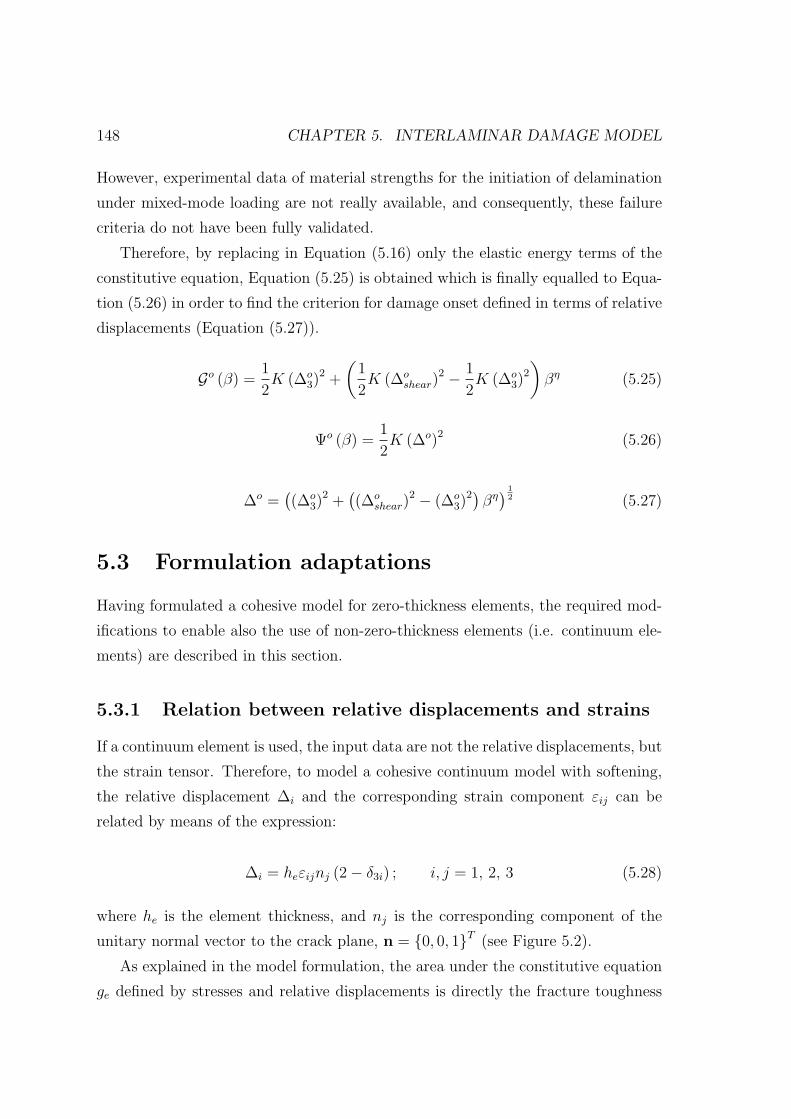
148 CHAPTER 5. INTERLAMINAR DAMAGE MODEL
However, experimental data of material strengths for the initiation of delamination
under mixed-mode loading are not really available, and consequently, these failure
criteria do not have been fully validated.
Therefore, by replacing in Equation (5.16) only the elastic energy terms of the
constitutive equation, Equation (5.25) is obtained which is finally equalled to Equa-
tion (5.26) in order to find the criterion for damage onset defined in terms of relative
displacements (Equation (5.27)).
Go (β) =1
2K (∆o
3)2 +
(1
2K (∆o
shear)2 − 1
2K (∆o
3)2
)βη (5.25)
Ψo (β) =1
2K (∆o)2 (5.26)
∆o =((∆o
3)2 +((∆o
shear)2 − (∆o
3)2) βη) 1
2 (5.27)
5.3 Formulation adaptations
Having formulated a cohesive model for zero-thickness elements, the required mod-
ifications to enable also the use of non-zero-thickness elements (i.e. continuum ele-
ments) are described in this section.
5.3.1 Relation between relative displacements and strains
If a continuum element is used, the input data are not the relative displacements, but
the strain tensor. Therefore, to model a cohesive continuum model with softening,
the relative displacement ∆i and the corresponding strain component εij can be
related by means of the expression:
∆i = heεijnj (2− δ3i) ; i, j = 1, 2, 3 (5.28)
where he is the element thickness, and nj is the corresponding component of the
unitary normal vector to the crack plane, n = 0, 0, 1T (see Figure 5.2).
As explained in the model formulation, the area under the constitutive equation
ge defined by stresses and relative displacements is directly the fracture toughness
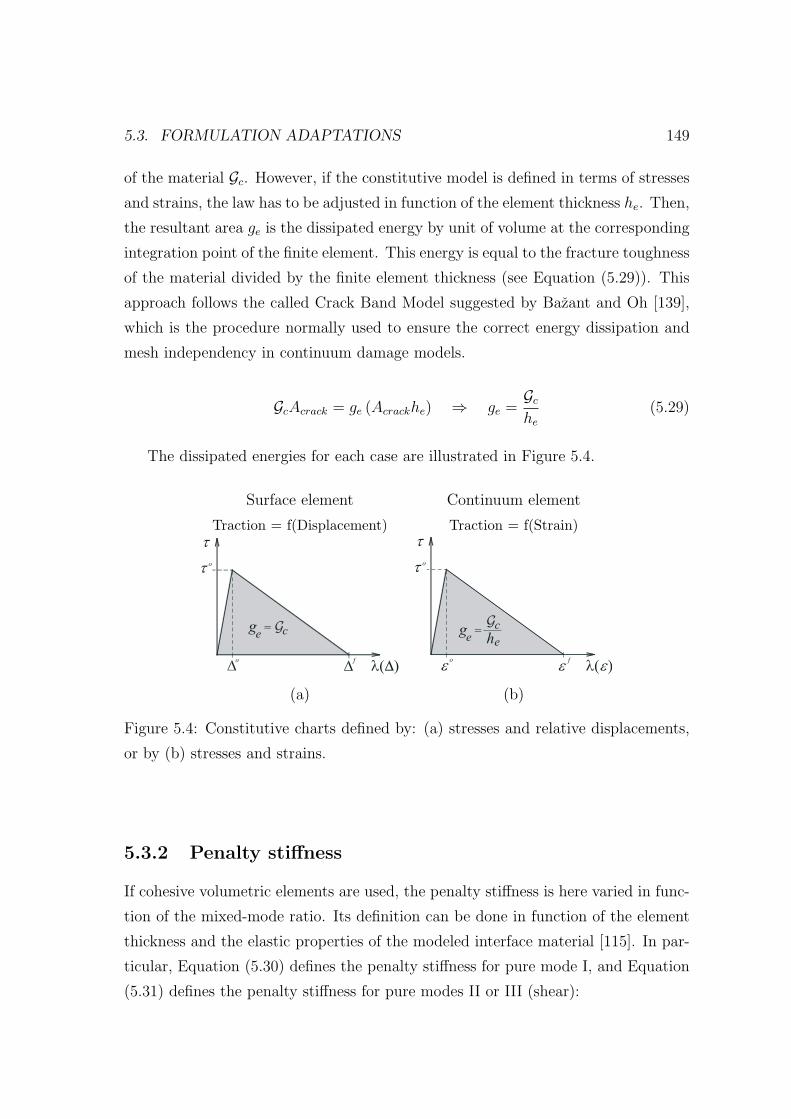
5.3. FORMULATION ADAPTATIONS 149
of the material Gc. However, if the constitutive model is defined in terms of stresses
and strains, the law has to be adjusted in function of the element thickness he. Then,
the resultant area ge is the dissipated energy by unit of volume at the corresponding
integration point of the finite element. This energy is equal to the fracture toughness
of the material divided by the finite element thickness (see Equation (5.29)). This
approach follows the called Crack Band Model suggested by Bazant and Oh [139],
which is the procedure normally used to ensure the correct energy dissipation and
mesh independency in continuum damage models.
GcAcrack = ge (Acrackhe) ⇒ ge =Gche
(5.29)
The dissipated energies for each case are illustrated in Figure 5.4.
Surface element Continuum element
Traction = f(Displacement) Traction = f(Strain)
(a) (b)
Figure 5.4: Constitutive charts defined by: (a) stresses and relative displacements,
or by (b) stresses and strains.
5.3.2 Penalty stiffness
If cohesive volumetric elements are used, the penalty stiffness is here varied in func-
tion of the mixed-mode ratio. Its definition can be done in function of the element
thickness and the elastic properties of the modeled interface material [115]. In par-
ticular, Equation (5.30) defines the penalty stiffness for pure mode I, and Equation
(5.31) defines the penalty stiffness for pure modes II or III (shear):

150 CHAPTER 5. INTERLAMINAR DAMAGE MODEL
K1 =Emhe
(5.30)
K2 =Gm
he(5.31)
where Em is the Young modulus and Gm is the shear elastic modulus of the interface
material. Normally, the elastic properties of the interface material are considered as
the neat material, although it is generally not true [125].
For surface cohesive elements, the penalty stiffness is selected with a fixed value
for all mixed-mode ratios. Ideally, the value of the penalty stiffness is infinite because
these elements do not have thickness, and then they do not affect the compliance
of the whole structure [140]. However, too high value of the interface stiffness can
generate numerical problems such as the generation of spurious oscillations in the
tractions of the element [114]. Therefore, a suitable value of the penalty stiffness
should be selected in order to provide a reasonable stiffness without generating
numerical problems. Based in mechanical considerations, Turon et al. [12] proposed
Equation (5.32) in order to estimate the interface stiffness K for mode I crack
propagation.
K =αE3
ha(5.32)
where E3 is the elastic modulus through-the-thickness of the composite material,
α is an increasing parameter (normally it is taken about α ≈ 50), and ha is the
laminate thickness adjoining to the cohesive element. Equation (5.32) also can be
developed for shear modes, by replacing E3 by the shear elastic modulus. However,
since the model formulation for surface elements assumes the same penalty stiffness
for each mixed-mode ratio, Equation (5.32) is used for all cases because it gives the
biggest value.
5.3.3 Redefined onset and propagation damage criteria
Since the penalty stiffness for the volumetric elements is a function of the mixed-
mode ratio, the onset and propagation damage criteria written in terms of relative
displacements must be redefined. However, the procedure used in Sections 5.2.3

5.3. FORMULATION ADAPTATIONS 151
and 5.2.4 to find these expressions can not be exactly applied here because the
function which describes the variation of the penalty stiffness under a determined
mixed-mode ratio is unknown.
In order to find the onset criterion, Equation (5.33) is used. This equation is the
damage criterion with the corresponding elastic energy terms replaced (i.e. Equation
(5.25) with different penalty stiffness for pure mode I and pure shear mode). On
the other hand, Equation (5.34) represents the elastic energy of the constitutive
equation defined in terms of relative displacements of pure mode I, ∆o3 (β), and pure
shear mode, ∆oshear (β), for damage onset in a determined mixed-mode ratio.
Go (β) =1
2K1 (∆o
3)2 +
(1
2K2 (∆o
shear)2 − 1
2K1 (∆o
3)2
)Bη (5.33)
Ψo (β) =1
2K1 〈∆o
3 (β)〉2 +1
2K2 (∆o
shear (β))2 (5.34)
Using Equation (5.33) and (5.34), and the selected definition of the mixed-mode
ratio (Equation (5.21)), the terms ∆o3 (β) and ∆o
shear (β) can be found:
〈∆o3 (β)〉 =
2Go (β)
K1 +(
β1−β
)K2
12
(5.35)
∆oshear (β) =
(β
1− β
) 12
〈∆o3 (β)〉 (5.36)
Finally, the onset damage criterion is obtained by taking the Euclidian norm
of the relative displacements described by Equations (5.35) and (5.36) (see Section
5.2.1):
∆o =(〈∆o
3 (β)〉2 + (∆oshear (β))2) 1
2 (5.37)
In the same sense, the propagation damage criterion can be deduced. In this
case, Equation (5.38) represents the damage criterion with the corresponding pure
fracture toughness terms replaced (i.e. Equation (5.22) with different penalty stiff-
ness for pure mode I and pure shear mode). On the other hand, Equation (5.39)
is the fracture toughness for a given mixed-mode ratio defined in terms of relative

152 CHAPTER 5. INTERLAMINAR DAMAGE MODEL
displacements for damage onset in pure modes I and shear, ∆o3 (β) and ∆o
shear (β),
and for damage propagation, ∆f3 (β) and ∆f
shear (β).
Gc (β) =1
2K1∆o
3∆f3 +
(1
2K2∆o
shear∆fshear −
1
2K1∆o
3∆f3
)Bη (5.38)
Gc (β) =1
2K1 〈∆o
3 (β)〉⟨
∆f3 (β)
⟩+
1
2K2 (∆o
shear (β))(
∆fshear (β)
)(5.39)
where ∆o3 (β) and ∆o
shear (β) are previously found by means of Equations (5.35) and
(5.36).
Equalling Equations (5.38) and (5.39), and using again the definition of the
mixed-mode ratio (Equation (5.21)), the terms ∆f3 (β) and ∆f
shear (β) can be found:
⟨∆f
3 (β)⟩
=K1 (1−Bη) ∆o
3∆f3 +K2B
η∆oshear∆
fshear
〈∆o3 (β)〉
(K1 +
(β
1−β
)K2
) (5.40)
∆fshear (β) =
(β
1− β
) 12 ⟨
∆f3 (β)
⟩(5.41)
Finally, the propagation damage criterion is obtained by making the Euclidian
norm of the relative displacements described by Equations (5.40) and (5.41) (see
Section 5.2.1):
∆f =
(⟨∆f
3 (β)⟩2
+(
∆fshear (β)
)2) 1
2
(5.42)
It should be noted that the B parameter must be redefined by Equation (5.43),
since the penalty stiffnesses in pure mode I and shear modes are different and then
they can not be simplified.
B =K2β
K2β +K1 (1− β)(5.43)
If Equations (5.30) and (5.31) are replaced in Equation (5.43), the B parameter
can be also defined in function of the elastic properties considered for the interface
material. That is:
B =Gmβ
Gmβ + Em (1− β)(5.44)

5.4. MODEL IMPLEMENTATION 153
5.4 Model implementation
5.4.1 Strategy of implementation
The delamination model presented by Turon et al. [9] was implemented in a user-
written element subroutine called UEL [124]. This implementation was used to
simulate problems in an implicit finite element code. However, the model formulated
in Sections 5.2 and 5.3 is here implemented in a user-written material subroutine,
called VUMAT, assigned for explicit finite element analysis.
The user material implemented has to be defined on sets of elements which
represent the delamination layers. These elements can be zero-thickness (i.e. sur-
face elements) or non-zero-thickness (i.e. continuum elements) types. In particular,
when a zero-thickness interface is used, in-plane cohesive elements with four inte-
gration points of the Abaqus element library must be used [122]. This element is
called COH3D8. However, when non-zero-thickness interface is desired, any tri-
dimensional solid element can be applied.
Figure 5.5: Transformations from strains to relative displacements for each propa-
gation mode.
When surface elements are used, the input data given by the finite element
software to the user material subroutine is directly the increment of the relative
displacement vector, whereas the input data for continuum elements is the incre-
ment of the strain tensor. In order to use the same subroutine for both element

154 CHAPTER 5. INTERLAMINAR DAMAGE MODEL
types, Equation (5.28) is applied to transform easily the corresponding strain tensor
components to relative displacements (see Figure 5.5). On the other hand, if surface
elements are used, a constitutive thickness equal to the unity has to be introduced in
the user material subroutine which ensures that the strains are equal to the relative
displacements.
5.4.2 Input variables to define the model
The parameters required to define completely the model in a user material subroutine
are described below:
• Elastic properties (isotropic) and density of the interface material: Em, νm
and ρm.
By means of Em and νm the value of Gm can be calculated by using Equation
(5.45). If surface elements are used, normally the value of Em is taken between
105 and 5×10⁶Nmm−3 for a sub-laminate thickness between 0.125mm and
5mm [12], and the Poisson coefficient νm must be equal to -0.5 in order to
obtain the same penalty stiffness for all mixed-mode ratios.
Gm =Em
2 (1 + νm)(5.45)
• Thickness of the interface cohesive element: he.
If surface elements are used, the value of the constitutive thickness introduced
in the subroutine must be equal to the unity (although the geometrical thick-
ness defined in the model is equal to zero).
• Interface strengths for pure mode I and pure shear modes (II and III): τ o3 and
τ o1 .
By means of the interface strengths, the relative displacements which give the
damage onset for pure mode loading cases are obtained. The corresponding
equations are:
∆o3 =
τ o3K1
(5.46)

5.4. MODEL IMPLEMENTATION 155
∆oshear =
τ o1K2
(5.47)
• Interface fracture toughness for pure mode I and shear modes (II and III): GIcand GIIc.The relative displacements which give the damage propagation for pure mode
loading cases are obtained by means of pure mode fracture toughnesses. The
corresponding equations are:
∆f3 =
2GIcK1∆o
3
=2GIcτ o3
(5.48)
∆fshear =
2GIIcK2∆o
shear
=2GIIcτ o1
(5.49)
• Parameter of the least-square fit: η.
The experimental data used to calculate η can be obtained from MMB tests
(Mixed-Mode Bending) at different mode ratios.
In a recent paper of Turon et al. [13], it was detected that changes in the
local mode ratio during the evolution of damage under mixed-mode loading can
cause errors in the determination of the energy dissipation and result in inaccurate
predictions of the global load-displacement response. This fact occurs even under
conditions where, according to Linear Elastic Fracture Mechanics, the global mode
ratio is constant (e.g. Mixed-Mode Bending Test (MMB)). This is a common dif-
ficulty in current formulations of the cohesive models. To solve this problem, an
engineering solution which relates the interlaminar strengths was proposed. It was
demonstrated that this relation yields to accurate predictions which ensures correct
energy dissipations when delamination propagates. This relation is defined as:
τ o1 = τ o3
√GIIcGIc
(5.50)
Therefore, seven input parameters are necessary in order to fed on the present
cohesive model: Em, νm, ρm, he, τo3 , GIc and GIIc.

156 CHAPTER 5. INTERLAMINAR DAMAGE MODEL
5.4.3 Algorithm
After to read the input parameters and to calculate the model constants (see previous
Sections 5.3.2 and 5.4.2), the steps of the algorithm which are repeated for each
stable time increment δt are numbered below:
1. Calculate the strain components at time t+ δt.
εit+δt
= εit + δεit+δt
i = 1, ..., 3 surface element
i = 1, ..., 6 volumetric element(5.51)
2. Calculate the relative displacements at time t+ δt for each propagation mode
(see Figure 5.5).
Mode I: ∆3t+δt =
heε1t+δt surface element
heε3t+δt volumetric element(5.52)
Mode II: ∆1t+δt =
heε2t+δt surface element
heγ13t+δt volumetric element(5.53)
Mode III: ∆2t+δt =
heε3t+δt surface element
heγ23t+δt volumetric element(5.54)
3. Application of the damage model, where the following terms are calculated:
∆sheart+δt =
√(∆1
t+δt
)2
+(
∆2t+δt
)2
(5.55)
λt+δt =
√⟨∆3
t+δt
⟩2
+(∆sheart+δt
)2(5.56)
βt+δt =∆2sheart+δt⟨
∆3t+δt
⟩2
+ ∆2sheart+δt
(5.57)
Bt+δt =K2βt+δt
K2βt+δt +K1 (1− βt+δt)(5.58)

5.4. MODEL IMPLEMENTATION 157
〈∆o3 (β)〉t+δt =
K1
(1−Bη
t+δt
)(∆o
3)2 +K2Bηt+δt (∆o
shear)2
K1 +(
βt+δt1−βt+δt
)K2
12
(5.59)
⟨∆f
3 (β)⟩t+δt
=K1
(1−Bη
t+δt
)∆o
3∆f3 +K2B
ηt+δt∆
oshear∆
fshear
〈∆o3 (β)〉t+δt
(K1 +
(βt+δt
1−βt+δt
)K2
) (5.60)
(∆oshear (β))t+δt =
(βt+δt
1− βt+δt
) 12
〈∆o3 (β)〉t+δt (5.61)
(∆fshear (β)
)t+δt
=
(βt+δt
1− βt+δt
) 12 ⟨
∆f3 (β)
⟩t+δt
(5.62)
∆ot+δt =
(〈∆o
3 (β)〉2t+δt + (∆oshear (β))2
t+δt
) 12 (5.63)
∆ft+δt =
(⟨∆f
3 (β)⟩2
t+δt+(
∆fshear (β)
)2
t+δt
) 12
(5.64)
G (∆t+δt) = min
∆ft+δt
(λt+δt −∆o
t+δt
)
λt+δt
(∆ft+δt −∆o
t+δt
) , 1
(5.65)
• If G (∆t+δt) ≤ dt ⇒ dt+δt = dt: elastic reloading, unloading or
neutral loading.
• If G (∆t+δt) > dt ⇒ dt+δt = G (∆t+δt): loading.
4. Calculate the stress vector at time t+ δt:
τt+δt = Ct+δtεt+δt (5.66)
where:

158 CHAPTER 5. INTERLAMINAR DAMAGE MODEL
• For surface elements:
Ct+δt =
(1− d∗t+δt
)Em 0 0
0 (1− dt+δt)Gm 0
0 0 (1− dt+δt)Gm
(5.67)
where:
d∗t+δt = dt+δt
⟨ε1t+δt
⟩∣∣ε1t+δt
∣∣ (5.68)
• For volumetric elements:
Ct+δt =
Em(1−(1−d∗t+δt)ν2m)
Υ−νmEm(−1−(1−d∗t+δt)νm)
Υ
−νmEm(−1−(1−d∗t+δt)νm)Υ
Em(1−(1−d∗t+δt)ν2m)
ΥνmEm(1−d∗t+δt)
Φ
νmEm(1−d∗t+δt)Φ
0 0
0 0
0 0
νmEm(1−d∗t+δt)Φ
0 0 0νmEm(1−d∗t+δt)
Φ0 0 0
−Em(1−d∗t+δt)(1−νm)
Φ0 0 0
0 Gm 0 0
0 0 (1− dt+δt)Gm 0
0 0 0 (1− dt+δt)Gm
(5.69)
where:
Φ = 1− 2ν2m
(1− d∗t+δt
)− νm (5.70)
Υ = 1− 2ν3m
(1− d∗t+δt
)− ν2
m
(3− 2d∗t+δt
)(5.71)

5.5. SIZE OF COHESIVE ELEMENTS 159
d∗t+δt = dt+δt
⟨ε3t+δt
⟩∣∣ε3t+δt
∣∣ (5.72)
5. Calculate the energy dissipated at time t+ δt:
Ξt+δt = Ξt + Ξδt (5.73)
where Ξt and Ξδt are the accumulated and the increment of the dissipated
energy, respectively. The determination of Ξδt is given by Equation (5.74):
Ξδt =1
2
(dt+δt − dt
δt
)(K1
(∆2
3t+δt+ ∆3t+δt
⟨−∆3t+δt
⟩)
+K2
(∆2
1t+δt+ ∆2
2t+δt
)) (5.74)
6. Calculate the free energy at time t+ δt:
Ψt+δt =1
2
((1− dt+δt)
(K2
(∆2
1t+δt+ ∆2
2t+δt
)+K1
(∆2
3t+δt
))
−1
2dt+δtK1
(∆3t+δt
⟨−∆3t+δt
⟩)) (5.75)
7. Calculate the internal energy at time t+ δt:
EIt+δt = Ψt+δt + Ξt+δt (5.76)
5.5 Size of cohesive elements
5.5.1 Maximum thickness of volumetric cohesive elements
For each mixed-mode ratio there is a maximum thickness of the cohesive elements
in the direction perpendicular to the crack propagation plane. This is due to the
fact that the propagation criterion defined in terms of relative displacements remains
constant and the onset criterion changes whether the element thickness changes. The
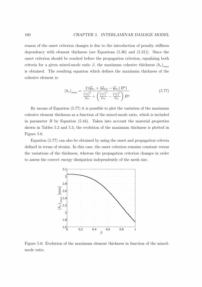
160 CHAPTER 5. INTERLAMINAR DAMAGE MODEL
reason of the onset criterion changes is due to the introduction of penalty stiffness
dependency with element thickness (see Equations (5.30) and (5.31)). Since the
onset criterion should be reached before the propagation criterion, equalizing both
criteria for a given mixed-mode ratio β, the maximum cohesive thickness (he)max
is obtained. The resulting equation which defines the maximum thickness of the
cohesive element is:
(he)max =2 (GIc + (GIIc − GIc)Bη)
(τo3 )2
Em+
((τo1 )
2
Gm− (τo3 )
2
Em
)Bη
(5.77)
By means of Equation (5.77) it is possible to plot the variation of the maximum
cohesive element thickness as a function of the mixed-mode ratio, which is included
in parameter B by Equation (5.44). Taken into account the material properties
shown in Tables 5.2 and 5.3, the evolution of the maximum thickness is plotted in
Figure 5.6.
Equation (5.77) can also be obtained by using the onset and propagation criteria
defined in terms of strains. In this case, the onset criterion remains constant versus
the variations of the thickness, whereas the propagation criterion changes in order
to assess the correct energy dissipation independently of the mesh size.
0 0.2 0.4 0.6 0.8 11.6
1.8
2
2.2
2.4
2.6
2.8
3
3.2
β
(he) m
ax
[mm
]
Figure 5.6: Evolution of the maximum element thickness in function of the mixed-
mode ratio.

5.5. SIZE OF COHESIVE ELEMENTS 161
Normally, the cohesive element thickness is defined with a small value (e.g. be-
tween 0.001 and 0.1mm) and certainly the value used will be smaller than the max-
imum value given by Equation (5.77).
Using again the material properties shown in Tables 5.2 and 5.3, the variation of
the onset criterion of the constitutive equation defined in terms of relative displace-
ments and the variation of the propagation criterion of the constitutive equation
chart defined in terms of strains are shown in Figure 5.7. These charts correspond
to the simulations in one element with constant in-plane dimensions under pure
mode I loading.
0 0.005 0.01 0.015 0.02 0.025 0.030
10
20
30
40
50
60
70
80
Displacement [mm]
Stre
ss [
MPa
]
0 0.01 0.02 0.03 0.04 0.05 0.060
10
20
30
40
50
60
70
80
Strain [mm]
Stre
ss [
MPa
]
he =0.5 mmhe =1.0 mmhe =2.0 mmhe =3.0 mm
(a) (b)
Figure 5.7: Constitutive equation charts defined by (a) relative displacements and
by (b) strains in function of the element thickness.
5.5.2 In-plane dimensions of the cohesive elements
The in-plane dimensions of the cohesive elements are selected following the consid-
erations and equations proposed by Turon et al. [12]. In particular, the in-plane
dimensions are defined by means of the cohesive zone length lcz, which is a material
and structural property [141]. It is defined as the distance from the crack front until
the point with the maximum interface strength τ o. To obtain suitable results by
using cohesive zone models, the tractions in the cohesive zone have to be represented
correctly by a proper number of elements.

162 CHAPTER 5. INTERLAMINAR DAMAGE MODEL
The model that will be used in this work in order to predict the length of the
cohesive zone was proposed by Rice [142], and reads:
lcz =9π
32Em
Gc (β)
(τ o (β))2 (5.78)
where Em is the Young modulus, and Gc (β) and τ o (β) are the fracture toughness and
the maximum strength of the interface for a given mixed-mode ratio, respectively.
The length of the cohesive elements le is easily calculated by means of:
le =lczNe
(5.79)
where Ne is the number of elements in the cohesive zone. Normally, the smallest
value of the cohesive zone length resulted from the different values of mixed-mode
ratio is used, and it is recommended to apply at least three or four elements in order
to describe the cohesive zone accurately.
5.6 Simulations
This section presents the application of cohesive elements in the simulation of inter-
laminar fracture tests of composite specimens under quasi-static loading conditions.
These tests allow the validation of the damage model presented without consider
the interaction with other damage mechanisms which can appear inside the plies,
because the damage is normally concentrated in interfaces where only delamination
occurs.
Mixed-Mode Bending (MMB) and End-Notched Flexure (ENF) tests of unidi-
rectional zero degree lay-up specimens with an initial pre-crack are considered (see
Section 5.6.2). The MMB allows to test any mixed-mode case except pure mode II,
which is obtained by the ENF test. The cases simulated are B = 0.0 (pure mode
I), B = 0.2, B = 0.5, B = 0.8 and B = 1.0 (pure mode II). It should be noted that
only non-zero-thickness elements have been used in all the simulations considered,
which represent a resin-rich interface layer.
Different mixed-mode analysis at one finite element were simulated previously
in order to check that the predicted dissipated energy at each integration point is

5.6. SIMULATIONS 163
equal to the corresponding fracture toughness adjusted by the least square fit of
experimental data points of the selected material (see Table 5.3).
Simulations of quasi-static Transverse Crack Tension tests (TCT) of unidirec-
tional zero degree lay-up specimens are also shown (see Section 5.6.3). The TCT
test is an alternative to the ENF test, which determines pure mode II interlaminar
fracture toughness [143].
Finally, the numerical considerations in order to carry out quasi-static simula-
tions by using an explicit finite element code are explained in detail.
5.6.1 Considerations for quasi-static explicit simulations
The proposed simulations are solved by means of an explicit finite element code.
As it has been explained in the introduction, the explicit integration schemes deter-
mine a solution to the dynamic equilibrium of the global set equations by explicitly
advancing the kinematic state from the previous time increment, without solving
simultaneously equations and without iterating for each time increment. For this
reason, the formulation of the tangent stiffness tensor is not derived here since no
iterations are carried out.
Static problems have a large time solution, which often it is unworkable to analyze
the simulation in its real scale of time using an explicit code because requires an
excessive number of stable small increments of time. To obtain a faster solution, the
event should be accelerated in some way, but ensuring that the inertial forces remain
insignificant. There are some actions to alter one or more of the factors influencing
the time increment. The action here considered for increasing the efficiency of the
proposed simulations is to scale the mass density of these critical elements (i.e. mass
scaling). In order to control the proposed simulations, the kinetic energy and the
internal energy are monitored in order to keep the kinetic energy less than 5% of
the internal energy of the system.
On the other hand, the loading velocity should be such that the solution obtained
is close to the real static solution and the dynamic effects remain insignificant. In
an approximate way, the maximum loading velocity vL can be estimated by means
of:

164 CHAPTER 5. INTERLAMINAR DAMAGE MODEL
vL < 0.01
√Emρm
(5.80)
The loading velocity defined in all the simulations is 0.5mm/s, which is much
lower than the maximum value given by Equation (5.80) (see interface properties in
Tables 5.3 and 5.6).
Quasi-static analysis in explicit algorithms require the application of loading as
smooth as possible. Sudden movements cause stress waves, which can introduce
noisy or inaccurate results. Applying the load in the smoothest possible manner
requires that the acceleration changes only a small amount from one time increment
to the next. Then, if the acceleration is smooth, it follows that the changes in
velocity and displacement are also smooth. This option can be defined easily in
Abaqus software by selecting a smooth amplitude table of loading in all the proposed
simulations. By defining it, Abaqus software connects automatically each of the user
data pairs of loading with curves, whose first and second derivatives are smooth, and
whose values are zero at each of user loading data points.
It has to be noted that the selected mass scaling factor for critical elements is
considerably high (i.e. approximately 10.03). However, since the boundary displace-
ments are applied in a smooth manner and in a large time scale, the kinetic energy
and the inertial forces of the model remain small.
Finally, the cohesive elements which reach the maximum damage value at their
integration points are deleted from the mesh. These deleted elements have no ability
to carry stresses and, therefore, have no contribution to the stiffness of the model.
This action avoids large distortions of the damaged elements, and possible spuri-
ous stress transfer to the bodies around them. However, if damaged elements are
deleted, penetration between the joined laminates can occur, mainly in tests with
high percentage of mode II. To avoid it, a contact pair surfaces without friction
have been defined between the two laminate surfaces that were initially linked by
the cohesive elements.
5.6.2 MMB and ENF fracture toughness tests
The simulations of quasi-static MMB and ENF tests of unidirectional zero degree
lay-up specimens are analyzed in this section.

5.6. SIMULATIONS 165
Test configurations
The loading conditions in the MMB simulations are defined by means of the linear
Equation (5.81) which relates the displacements in three different points of the
specimen [118]:
δLP =( cL
)δI +
(c+ L
L
)δM (5.81)
where L is the half specimen length and c is the length from the loading point LP to
the middle point M of the specimen. The different mixed-mode cases are generated
by modifying the length c, which reads:
c =L(
12
√3(
1−BB
)+ 1)
3− 12
√3(
1−BB
) (5.82)
In Figure 5.8.a are marked the points LP , M , and I where the displacements
are prescribed.
(a) (b)
Figure 5.8: Sketches of the (a) MMB test and the (b) ENF test configurations.
The loading conditions of the ENF test are also defined by displacements. Just
as indicates Figure 5.8.b, it is applied a displacement in the middle point M of the
specimen.
The numerical results are compared with experimental data performed by Reeder
and Crews [144–146] to validate the model. These results are presented in a force-
displacement chart. For the MMB test, the results are read at point LP , and in
point M for the ENF test.

166 CHAPTER 5. INTERLAMINAR DAMAGE MODEL
Sizes and types of the elements
An 8-node solid element with reduced integration (one integration point) is used
to model the laminates and volumetric cohesive elements. This element is called
C3D8R. For all simulations, each laminate thickness is modeled by four elements,
which is enough to capture accurately the laminate rotations during the simulations.
The thickness defined for the interface elements is 0.01mm, which is much smaller
than the value obtained by means of Equation (5.77) (see Figure 5.6).
On the other hand, the in-plane length of the cohesive element is determined
by Equations (5.78) and (5.79). If three elements are desired to be along the cohe-
sive length, the maximum in-plane length at the crack propagation direction is of
0.45mm. The length finally used is 0.3mm for all the simulations. It is not neces-
sary to define a small length element at width specimen direction because the crack
propagates on the opposite direction. Therefore, the specimen width is modeled by
using only two elements.
Materials and specimen dimensions
The material used is a thermoplastic matrix-based reinforced by unidirectional car-
bon fibers (AS4/PEEK). The properties are set in Table 5.1:
Table 5.1: AS4/PEEK properties.
E1 [MPa] E2 = E3 [MPa] G12 = G13 [MPa] G23 [MPa] ν12 = ν13 ν23 ρ [tmm−3]
122700 10100 5500 3700 0.25 0.45 1600e-12
The material properties defined to the interface elements are summarized in
Table 5.2, and are selected by considering that these elements represent a resin-rich
layer. The pure mode fracture toughnesses of the interface are written in Table 5.3.
The shear strength τ o1 is defined by means Equation (5.50), which yields to 106MPa.
The parameter η is taken 2.284, which is obtained by means of a least-square fit
of the experimental data shown in Table 5.3.
The specimen dimensions are: 102mm long, 25.4mm wide, and each laminate
arm is 1.56mm thick.

5.6. SIMULATIONS 167
Table 5.2: Interface properties.
Em [MPa] νm ρm [tmm−3] τ o3 [MPa]
10100 0.3 1600e-12 80
Table 5.3: Fracture toughnesses of the interface for different mixed-mode ratios
[145, 146].GIIGT
0% 20% 50% 80% 100% (ENF)
Gc [N/mm] 0.969 1.103 1.131 1.376 1.719
ac0 [mm] 32.9 33.7 34.1 31.4 39.2
Results
The force-displacement relations obtained in the experiments and in the finite el-
ement simulations of the MMB test for each proposed mixed-mode case: B = 0.0
(pure mode I), B = 0.2, B = 0.5, and B = 0.8 are respectively shown in Figures
5.9, 5.10, 5.11, and 5.12. The results of the ENF test (B = 1.0, pure mode II) are
shown in Figure 5.13.
The corresponding analytical expressions for MMB test with B = 0.0 (pure mode
I) and ENF test which give the relationship of the critical load and the displacement
during propagation are also plotted in the corresponding figures. These equations
are set in Table 5.4, and are deduced by using Linear Elastic Fracture Mechanics and
Simple Beam Theory [147, 148]. In these equations, E1 is the longitudinal elastic
modulus of the specimen, ac is the crack length, and b, ha and L are the width, the
arm height and the half length of the specimen, respectively.
Table 5.4: Analytical equations of MMB test with B = 0.0, and ENF test (B = 1.0).
Test Critical load Compliance
MMB (B = 0.0) Pc =√
E1b2h3aGIc
12a2c
C = 8a3c
E1bh3a
ENF (B = 1.0) Pc =√
16E1b2h3aGIIc
9a2c
C = 3a3c+2L3
8E1bh3a

168 CHAPTER 5. INTERLAMINAR DAMAGE MODEL
0 2 4 6 80
50
100
150
Displacement [mm]
Forc
e [N
]
ExperimentalNumericalAnalytical
Figure 5.9: Experimental and numerical force-displacement relation of the MMB
test B = 0.0 (pure mode I).
0 2 4 6 8 10 120
20
40
60
80
100
120
Displacement [mm]
Forc
e [N
]
ExperimentalNumerical
Figure 5.10: Experimental and numerical force-displacement relation of the MMB
test B = 0.2.
Discussion
The charts obtained by numerical simulations of the proposed tests are in a good
agreement with the experimental data. The predicted case of B = 0.0 (pure mode I)
is the most far of the corresponding experimental chart. This difference is not due to
limitations of the numerical simulations, but rather to the fact that the experimental

5.6. SIMULATIONS 169
0 1 2 3 4 5 60
50
100
150
200
250
300
Displacement [mm]
Forc
e [N
]
ExperimentalNumerical
Figure 5.11: Experimental and numerical force-displacement relation of the MMB
test B = 0.5.
0 1 2 3 4 5 60
100
200
300
400
500
600
Displacement [mm]
Forc
e [N
]
ExperimentalNumerical
Figure 5.12: Experimental and numerical force-displacement relation of the MMB
test B = 0.8.
fracture toughness used corresponds to the onset delamination and not to the prop-
agation, which is normally larger than the onset fracture toughness. The analytical
model which gives the relationship of the critical load and the displacement during
propagation is plotted. The fracture toughness specified is Gc = 0.969N/mm (see
Table 5.3), and the numerical curve shows an excellent correlation with the descend-
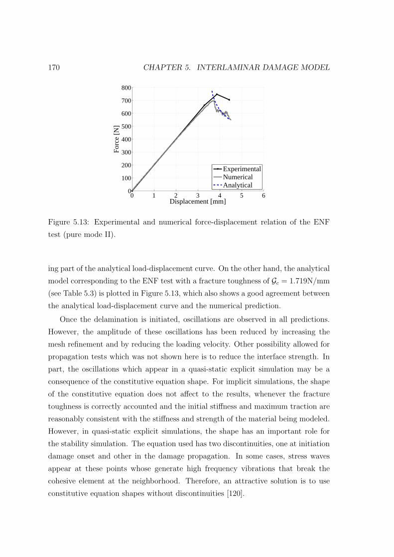
170 CHAPTER 5. INTERLAMINAR DAMAGE MODEL
0 1 2 3 4 5 60
100
200
300
400
500
600
700
800
Displacement [mm]
Forc
e [N
]
ExperimentalNumericalAnalytical
Figure 5.13: Experimental and numerical force-displacement relation of the ENF
test (pure mode II).
ing part of the analytical load-displacement curve. On the other hand, the analytical
model corresponding to the ENF test with a fracture toughness of Gc = 1.719N/mm
(see Table 5.3) is plotted in Figure 5.13, which also shows a good agreement between
the analytical load-displacement curve and the numerical prediction.
Once the delamination is initiated, oscillations are observed in all predictions.
However, the amplitude of these oscillations has been reduced by increasing the
mesh refinement and by reducing the loading velocity. Other possibility allowed for
propagation tests which was not shown here is to reduce the interface strength. In
part, the oscillations which appear in a quasi-static explicit simulation may be a
consequence of the constitutive equation shape. For implicit simulations, the shape
of the constitutive equation does not affect to the results, whenever the fracture
toughness is correctly accounted and the initial stiffness and maximum traction are
reasonably consistent with the stiffness and strength of the material being modeled.
However, in quasi-static explicit simulations, the shape has an important role for
the stability simulation. The equation used has two discontinuities, one at initiation
damage onset and other in the damage propagation. In some cases, stress waves
appear at these points whose generate high frequency vibrations that break the
cohesive element at the neighborhood. Therefore, an attractive solution is to use
constitutive equation shapes without discontinuities [120].

5.6. SIMULATIONS 171
5.6.3 TCT tests
The simulations of quasi-static Transverse Crack Tension tests (TCT) of unidirec-
tional zero degree lay-up specimens are analyzed in this section.
Configuration of the TCT tests
The TCT specimens are manufactured by continuous fiber laminates with unidirec-
tional stacking order whose central plies are cut prior to curing, as shown in Figure
5.14. When these specimens are loaded by tension, delaminations develop under
pure mode II. Such laminates are referred by [0m, ∅n]S, where the slash indicates the
cut plies.
Figure 5.14: TCT specimen.
The TCT specimens can be tested with or without pre-cracks previously induced.
The specimens with pre-cracks are those undergoing a determined number of fatigue
cycles at near-threshold loading for delamination growth. For no pre-cracked spec-
imens, the gap between cut plies is a resin rich region which delaminates under
pure mode I. Next, at certain load level, delamination starts at the corner point be-
tween cut and continuous plies along the fiber direction and quickly develops under
pure mode II to certain length or full-scale. For pre-cracked specimens, this pre-
delamination phase is not experimented since small initial interface cracks are previ-
ously created [149]. Consequently, the resulting critical load and fracture toughness
are more representative in these specimens than for no pre-cracked specimens.

172 CHAPTER 5. INTERLAMINAR DAMAGE MODEL
The TCT test is then an alternative to the ENF test [150]. It is assumed that in
the TCT test there is less sliding friction between the delaminated plies than in the
ENF test. A second advantage concerns compliance calibration for data reduction.
The compliance of the TCT specimen is less sensitive to the error in crack length
measurement, because the compliance is related linearly to the crack length ac (see
Equation (5.83)), whereas for the ENF specimen the compliance is related to a3c (see
Table 5.4).
C =L (h− hc) + 2achcbh (h− hc)E1
(5.83)
E1 is the longitudinal elastic modulus of the specimen, and hc is the whole thickness
of cut central plies. The geometrical variables L, b and h are the length, width, and
total thickness of the specimen, respectively.
From the evaluation of the compliance C and the delamination length ac, the
fracture toughness GIIc can be derived for a constant specimen width b as:
GIIc =1
4
hcP2c
b2E1h (h− hc)(5.84)
The factor 1/4 is introduced because there are four crack tips. Equation (5.84)
shows that GIIc can be obtained by determining solely the critical load Pc.
Only non pre-cracked specimens are simulated. The laminates considered are:
[02, ∅4]S, [04, ∅4]S and [04, ∅8]S. The numerical results obtained are basically the
critical load Pc for delamination propagation, and are compared with experimental
values performed by Ye et al. [149].
Sizes and types of the elements
Two delamination planes are modeled in the TCT specimens, as shown in Figure
5.15. One corresponds to the interface of the cut central plies which delaminates
under pure mode I, and is modeled by using zero-thickness type elements with four
integration points of the Abaqus element library (i.e. COH3D8). The other delam-
ination plane corresponds to the interface between cut and continuous plies along
the fiber direction which delaminates under pure mode II. In this case, the interface
is modeled by using non-zero-thickness type elements with reduced integration (i.e.

5.6. SIMULATIONS 173
C3D8R). The thickness defined for this interface is 0.01mm, which is much smaller
than the value obtained by means of Equation (5.77). The in-plane length of these
elements at the crack propagation direction is determined by means of Equations
(5.78) and (5.79). If three elements are desired to be along the cohesive length, the
maximum in-plane length is of 0.37mm. The length finally used is 0.33mm.
The specimen width is meshed with five elements, and each ply thickness with
two elements. The composite material is modeled by using also C3D8R elements.
Only half thickness of the specimen is modeled by defining symmetric boundary
conditions.
Figure 5.15: Detail of the location of the cohesive elements.
Materials and specimen dimensions
The composite material used is an epoxy matrix-based reinforced by unidirectional
carbon fibers (T300/914C). The properties are extracted from Ye et al. [149] and
set in Table 5.5.
The material properties defined to the interface elements located between cut
and continue plies are shown in Table 5.6, and are selected by considering that
these elements represent a resin-rich layer. The fracture toughness GIIc is obtained
by testing pre-cracked TCT specimens. For zero-thickness cohesive elements the
properties are equal than those set in Table 5.6 except the elastic modulus (i.e.
penalty stiffness) which is set 106, and in order to obtain the same penalty stiffness
for all propagation modes the Poisson modulus is set equal to -0.5. The shear
strength τ o1 is defined by means Equation (5.50), which yields to 83MPa.
The parameter η is approached to 1.47, which is obtained by means of least-
square fit of mixed-mode fracture toughnesses obtained in MMB tests [150]. The
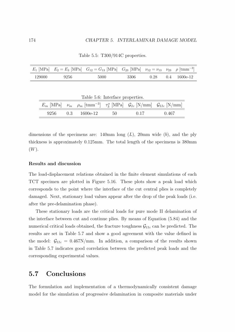
174 CHAPTER 5. INTERLAMINAR DAMAGE MODEL
Table 5.5: T300/914C properties.
E1 [MPa] E2 = E3 [MPa] G12 = G13 [MPa] G23 [MPa] ν12 = ν13 ν23 ρ [tmm−3]
129000 9256 5000 3306 0.28 0.4 1600e-12
Table 5.6: Interface properties.
Em [MPa] νm ρm [tmm−3] τ o3 [MPa] GIc [N/mm] GIIc [N/mm]
9256 0.3 1600e-12 50 0.17 0.467
dimensions of the specimens are: 140mm long (L), 20mm wide (b), and the ply
thickness is approximately 0.125mm. The total length of the specimens is 380mm
(W ).
Results and discussion
The load-displacement relations obtained in the finite element simulations of each
TCT specimen are plotted in Figure 5.16. These plots show a peak load which
corresponds to the point where the interface of the cut central plies is completely
damaged. Next, stationary load values appear after the drop of the peak loads (i.e.
after the pre-delamination phase).
These stationary loads are the critical loads for pure mode II delamination of
the interface between cut and continue plies. By means of Equation (5.84) and the
numerical critical loads obtained, the fracture toughness GIIc can be predicted. The
results are set in Table 5.7 and show a good agreement with the value defined in
the model: GIIc = 0.467N/mm. In addition, a comparison of the results shown
in Table 5.7 indicates good correlation between the predicted peak loads and the
corresponding experimental values.
5.7 Conclusions
The formulation and implementation of a thermodynamically consistent damage
model for the simulation of progressive delamination in composite materials under
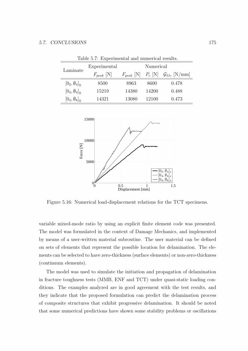
5.7. CONCLUSIONS 175
Table 5.7: Experimental and numerical results.
LaminateExperimental Numerical
Fpeak [N] Fpeak [N] Pc [N] GIIc [N/mm]
[02, ∅4]S 8500 8963 8600 0.478
[04, ∅4]S 15219 14380 14200 0.488
[04, ∅8]S 14321 13080 12100 0.473
0 0.5 1 1.50
5000
10000
15000
Displacement [mm]
Forc
e [N
]
[02, ∅4]s[04, ∅4]s[04, ∅8]s
Figure 5.16: Numerical load-displacement relations for the TCT specimens.
variable mixed-mode ratio by using an explicit finite element code was presented.
The model was formulated in the context of Damage Mechanics, and implemented
by means of a user-written material subroutine. The user material can be defined
on sets of elements that represent the possible location for delamination. The ele-
ments can be selected to have zero-thickness (surface elements) or non-zero-thickness
(continuum elements).
The model was used to simulate the initiation and propagation of delamination
in fracture toughness tests (MMB, ENF and TCT) under quasi-static loading con-
ditions. The examples analyzed are in good agreement with the test results, and
they indicate that the proposed formulation can predict the delamination process
of composite structures that exhibit progressive delamination. It should be noted
that some numerical predictions have shown some stability problems or oscillations

176 CHAPTER 5. INTERLAMINAR DAMAGE MODEL
which have been reduced significantly by increasing the mesh refinement and by
reducing the loading velocity during the crack propagation process. However, these
oscillations may be reduced even more by modifying the shape of the constitutive
equation to one without discontinuity points.
To make use of the damage model implemented and of the explicit finite ele-
ment code, the next step is to simulate low-velocity impacts of foreign objects on
monolithic laminated composite plates, where the delamination generally propagates
under variable mixed-mode conditions (see Chapter 7). In these analysis, the study
of the shape and extension of the delamination at interfaces between mismatch ori-
entation plies is of great interest since the delamination reduces dramatically the
damage tolerance of the structure. In order to carry out an accurately prediction, an
intralaminar damage model must be added in these analysis (see Chapter 6), since
impact loading conditions creates intralaminar damage mechanisms which interact
with the delamination failure mode.
Chapter 6
Intralaminar damage model
6.1 Introduction
Strength-based failure criteria can be used to predict the onset of the damage mech-
anisms which contribute to final failure of a composite structure. However, these
criteria are inaccurate in predicting the ultimate structural failure of composite
structures that can accumulate damage before final collapse. Continuum Damage
Mechanics is a more accurate methodology to predict the quasi-brittle failure of
composites, from the onset up to final collapse. The prediction of the damage accu-
mulation is a key information since it defines the damage tolerance and the eventual
collapse of a structure.
The intralaminar damage model developed by Maimı et al. [14–17] is summarized
in the present chapter. This model accounts the matrix cracking and the fiber
breakage damage mechanisms for 3D plies, and will be used, together with the
delamination damage model presented in Chapter 5, for the simulation of the impact
and the CAI tests in Abaqus/Explicit finite element code [124].
The model is developed in the context of the mechanics of continuum mediums,
using a rigorous thermodynamic framework where the irreversibility of the damage
processes are ensured. The main features of the model are listed below:
• The majority of the material properties required for the definition of the dam-
age model can be measured using standard ply-based test methods.
• The damage activation functions, which predict the different failure mech-
177

178 CHAPTER 6. INTRALAMINAR DAMAGE MODEL
anisms occurring at the ply level, are based mainly on the LaRC04 failure
criteria [76, 77]. This criteria accounts for the in-situ effect of the thickness of
a ply on its transverse tensile and shear strengths.
• The model accounts for crack-closure effects under load reversal conditions.
The consideration of these effects are significant in structures that are sub-
jected to multi-axial loading, such as in the impact and the CAI tests.
• The objectivity of the finite element model is ensured using the crack band
model proposed by Bazant and Oh [139], by regularizing the computed dis-
sipated energy of each failure mechanism using a characteristic dimension of
the finite element and the corresponding fracture toughness.
Finally, simple FE simulations which illustrate the well-known limitations of
using a continuum damage model for capturing matrix macro-crack paths in absence
of fiber breakage are shown.
6.2 Continuum damage model
6.2.1 Constitutive model
The constitutive equation is obtained by the definition of a thermodynamic poten-
tial. In this case, the complementary free energy density is used, and it is defined
as:
G =σ2
11
2 (1− d1)E1
+σ2
22
2 (1− d2)E2
+σ2
33
2 (1− d3)E2
− ν12
E1
σ11(σ22 + σ33)−
−ν23
E2
σ22σ33 +σ2
23
2 (1− d4)G23
+σ2
13
2 (1− d5)G12
+
+ (α11σ11 + α22(σ22 + σ33)) ∆T + (β11σ11 + β22(σ22 + σ33)) ∆M
(6.1)
where E1, E2, ν12 and G12 are the in-plane elastic properties of a unidirectional lam-
ina. The damage variable d1 is associated with longitudinal (fiber) failure, whereas
d2 and d3 are the damage variables associated with transverse (matrix cracking)
failure controlled by in-plane and out-of-plane loads, respectively. The damage vari-
ables d4, d5, and d6 are influenced by longitudinal and transverse cracks. α11 and α22

6.2. CONTINUUM DAMAGE MODEL 179
are the coefficients of thermal expansion in the longitudinal and transverse direc-
tions, respectively. β11 and β22 are the coefficients of hygroscopic expansion in the
longitudinal and transverse directions, respectively. ∆T and ∆M are the differences
of temperature and moisture content with respect to the corresponding reference
values.
By ensuring the thermodynamical irreversibility of the damage process, the
constitutive relationship of strains, ε = ε11, ε22, ε33, ε12, ε13, ε23T , and stresses,
σ = σ11, σ22, σ33, σ12, σ13, σ23T , can be found:
ε =∂G
∂σ= H : σ + α∆T + β∆M (6.2)
where the lamina compliance tensor H = ∂2G∂σ⊗∂σ
is defined as:
H =
1(1−d1)E1
−ν12E1
−ν12E1
0 0 0
−ν12E1
1(1−d2)E2
−ν23E2
0 0 0
−ν12E1
−ν23E2
1(1−d3)E2
0 0 0
0 0 0 1(1−d6)G12
0 0
0 0 0 0 1(1−d5)G12
0
0 0 0 0 0 1(1−d4)G23
(6.3)
The closure of transverse cracks under load reversal, is taken into account mak-
ing:
d1 = d1+〈σ11〉|σ11|
+ d1−〈−σ11〉|σ11|
d2 = d2+〈σ22〉|σ22|
+ d2−〈−σ22〉|σ22|
(6.4)
where 〈x〉 is the Macaulay operator defined as 〈x〉 := 12
(x+ |x|). The model tracks
damage caused by tension loads (d+) separately from damage caused by compression
loads (d−). The model assumes that the shear damage variables are not affected by
the closure effect.

180 CHAPTER 6. INTRALAMINAR DAMAGE MODEL
6.2.2 Damage activation functions
The elastic domain is enclosed by four surfaces, each of them accounts one failure
mechanism: longitudinal and transverse fracture under tension and compression.
Those surfaces are formulated by the damage activation functions based on the
LaRC04 failure criteria, neglecting the out-of-plane stresses. These damage activa-
tion functions FN , associated with damage in the longitudinal (N = 1+, 1−) and
transverse (N = 2+, 2−) directions represented in Figure 6.1, are defined as:
F1+ = φ1+ − r1+ ≤ 0 ; F1− = φ1− − r1− ≤ 0
F2+ = φ2+ − r2+ ≤ 0 ; F2− = φ2− − r2− ≤ 0
(6.5)
where the loading functions φN (N = 1+, 1−, 2+, 2−) depend on the strain ten-
sor and material constants (elastic and strength properties). The elastic domain
thresholds rN (N = 1+, 1−, 2+, 2−) take an initial value of 1 when the material
is undamaged, and they increase with damage. The elastic domain thresholds are
internal variables of the constitutive model, and are related to the damage variables
dM (M = 1+, 1−, 2+, 2−, 6) by the damage evolution laws.
(a) Longitudinal tensile fracture. (b) Longitudinal compressive fracture.
(c) Transverse fracture (α0 = 0). (d) Transverse fracture (α0 = 53).
Figure 6.1: Fracture surfaces and corresponding internal variables for four different
modes.
The elastic domain thresholds rN define the level of elastic strains that can be at-
tained before the accumulation of additional damage. The elastic domain thresholds

6.2. CONTINUUM DAMAGE MODEL 181
are obtained applying the Kuhn-Tucker and consistency conditions. Considering the
effect of the cracks when load reversal occurs, the elastic domain thresholds are:
rN+ = max
1,max
s=0,t
φsN+
,maxs=0,t
φsN−
; N = 1, 2
rN− = max
1,max
s=0,t
φsN−
; N = 1, 2
(6.6)
Longitudinal tensile fracture
The LaRC04 criterion for fiber tension failure is a maximum allowable strain criterion
defined as:
φ1+ =E1
XT
ε11 =σ11 − ν12σ22
XT
(6.7)
whereXT is the tensile strength of the fiber. The effective stress tensor σ is computed
as σ = H0−1 : ε. H0 is the undamaged compliance tensor obtained from Equation
(6.3) using dN = 0 (N = 1, 2, . . . , 6).
Longitudinal compressive fracture
The damage activation function used to predict damage under longitudinal com-
pression (σ11 < 0) and in-plane shear (fiber kinking) is established as a function of
the components of the stress tensor σ(m) in a coordinate system (m) representing
the fiber misalignment:
φ1− =
⟨|σm12|+ ηLσm22
⟩
SL(6.8)
where the longitudinal friction coefficient ηL can be approximated as [76]:
ηL ≈ −SL cos (2α0)
YC cos2 α0
(6.9)
with α0 = 53. The components of the effective stress tensor in the coordinate
system associated with the rotation of the fibers are calculated as [76]:
σm22 = σ11 sin2 ϕC + σ22 cos2 ϕC − 2 |σ12| sinϕC cosϕC
σm12 = (σ22 − σ11) sinϕC cosϕC + |σ12|(cos2 ϕC − sin2 ϕC
) (6.10)

182 CHAPTER 6. INTRALAMINAR DAMAGE MODEL
The misalignment angle ϕC is determined using standard shear and longitudinal
compression strengths, SL and XC , respectively [76]:
ϕC = arctan
1−√
1− 4(SLXC
+ ηL)
SLXC
2(SLXC
+ ηL)
(6.11)
Transverse fracture perpendicular to the mid-plane of the ply
Transverse matrix cracks perpendicular to the mid-plane of the ply, i.e. with α0 =
0, are created by a combination of in-plane shear stresses and transverse tensile
stresses, or in-plane shear stresses and small transverse compressive stresses. These
conditions are represented by the following failure criteria:
φ2+ =
√(1− g)
σ22
YT+ g
(σ22
YT
)2
+
(σ12
SL
)2
if σ22 ≥ 0
1
SL
⟨|σ12|+ ηLσ22
⟩if σ22 < 0
(6.12)
where YT is the transverse tensile strength, and g is the fracture toughness ratio
defined as g = G2+/G6. G2+ is the transverse tensile fracture toughness, and G6 is
the shear fracture toughness.
Transverse compressive fracture
The matrix failure criterion for transverse compressive stresses consists of a quadratic
interaction between the effective shear stresses acting on the fracture plane:
φ2− =
√(τTeff
ST
)2
+
(τLeff
SL
)2
if σ22 < 0 (6.13)
where the effective stresses τTeff and τLeff are computed as [76]:
τTeff =⟨−σ22 cos (α0)
(sin (α0)− ηT cos (α0) cos (θs)
)⟩
τLeff =⟨cos (α0)
(|σ12|+ ηLσ22 cos (α0) sin (θs)
)⟩ (6.14)

6.2. CONTINUUM DAMAGE MODEL 183
with θs = arctan(−|σ12|
σ22 sin(α0)
)(sliding angle), ηT = −1
tan(2α0)(coefficient of transverse
influence), and ST = YC cos (α0)[sin (α0) + cos(α0)
tan(2α0)
](transverse shear strength).
6.2.3 Damage evolution laws
The internal variables rN define the threshold of the elastic domains, and are related
to the damage variables by means of the damage evolution laws. These laws are
expressed in the following general form:
dM = 1− 1
fN (rN)exp AM [1− fN (rN)] ; M = 1+, 1−, 2+, 2−, 6 (6.15)
where the function fN (rN) (N = 1+, 1−, 2+, 2−) is selected to force the softening
of the constitutive relation.
The parameters AM (M = 1+, 1−, 2+, 2−, 6) are calculated to ensure that the
computed density of the dissipated energy gM is independent of the finite element
size, hence it is selected to accomplish the following condition for all failure modes:
gM =
∫ ∞
1
∂G
∂dM
∂dM∂rM
drN =GM`∗
; M = 1+, 1−, 2+, 2−, 6 (6.16)
where `∗ is the characteristic finite element length.
In detail, the damage evolution laws and the corresponding related parameters
are listed below:
• Longitudinal tension. The longitudinal tension damage evolution law fol-
lows a linear-exponential law to consider the process of fiber-matrix failure
followed by fiber bridging and fiber pull-out. The softening is linear until the
stress reaches the pull-out stress XPO, and the corresponding energy dissipa-
tion per unit area is GL1+. As the strains continue to increase, the softening
response follows an exponential law and the energy dissipated per unit area is
GE1+. The corresponding damage evolution law is defined as:
d1+ = 1−(1− dL1+
) (1− dE1+
)(6.17)
where:
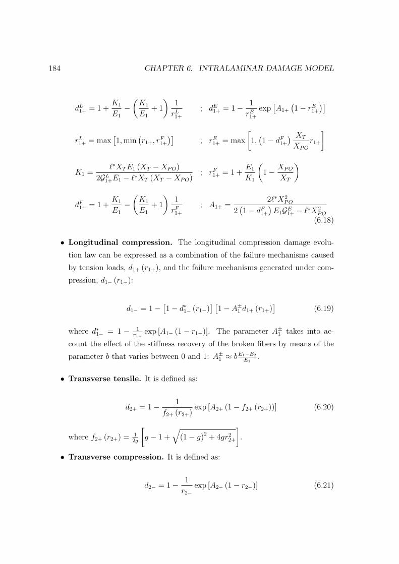
184 CHAPTER 6. INTRALAMINAR DAMAGE MODEL
dL1+ = 1 +K1
E1
−(K1
E1
+ 1
)1
rL1+
; dE1+ = 1− 1
rE1+
exp[A1+
(1− rE1+
)]
rL1+ = max[1,min
(r1+, r
F1+
)]; rE1+ = max
[1,(1− dF1+
) XT
XPO
r1+
]
K1 =`∗XTE1 (XT −XPO)
2GL1+E1 − `∗XT (XT −XPO); rF1+ = 1 +
E1
K1
(1− XPO
XT
)
dF1+ = 1 +K1
E1
−(K1
E1
+ 1
)1
rF1+
; A1+ =2`∗X2
PO
2(1− dF1+
)E1GE1+ − `∗X2
PO
(6.18)
• Longitudinal compression. The longitudinal compression damage evolu-
tion law can be expressed as a combination of the failure mechanisms caused
by tension loads, d1+ (r1+), and the failure mechanisms generated under com-
pression, d1− (r1−):
d1− = 1−[1− d∗1− (r1−)
] [1− A±1 d1+ (r1+)
](6.19)
where d∗1− = 1 − 1r1−
exp [A1− (1− r1−)]. The parameter A±1 takes into ac-
count the effect of the stiffness recovery of the broken fibers by means of the
parameter b that varies between 0 and 1: A±1 ≈ bE1−E2
E1.
• Transverse tensile. It is defined as:
d2+ = 1− 1
f2+ (r2+)exp [A2+ (1− f2+ (r2+))] (6.20)
where f2+ (r2+) = 12g
[g − 1 +
√(1− g)2 + 4gr2
2+
].
• Transverse compression. It is defined as:
d2− = 1− 1
r2−exp [A2− (1− r2−)] (6.21)

6.2. CONTINUUM DAMAGE MODEL 185
• In-plane shear. The shear stress stiffness is reduced as a result of longitudinal
and transverse cracks:
d6 = 1− [1− d∗6 (r2+)] (1− d1+) (6.22)
where:
d∗6 (r2+) = 1− 1
r2+
exp [A6 (1− r2+)]
A6 =2`∗S2
L
2G12G6 − `∗S2L
(6.23)
The parameters A1−, A2+ and A2− are calculated numerically using the algo-
rithms proposed in [15]. Finally, the out-of-plane damage variables are defined as:
d3 (r1−, r2−) = 1− [1− d1−(r1−)] [1− d2−(r2−)]
d4 (r2+) = d6 (r2+)
d5 (r1+) = d1 (r1+)
(6.24)
6.2.4 Maximum in-plane finite element size
The slope of the softening law for each damage mode is determined to dissipate the
correct energy according to the element size, i.e. the area under the stress-strain
chart is the corresponding fracture toughness divided by the finite element char-
acteristic length GM/`∗ (M = 1+, 1−, 2+, 2−, 6), see Equation (6.16). In order to
avoid snap-back of the softening branch for each failure mode, a maximum char-
acteristic element length `∗max can be found by equaling the elastic energy of the
element, 12XMεM(`∗)2hel = 1
2XMEM
2(`∗)2hel, with the energy dissipated in the fracture
process, GM`∗hel:
`∗max =2EMGMX2M
; M = 1+, 1−, 2+, 2−, 6 (6.25)
where hel is the element thickness. EM , GM , and XM , are, respectively, the Young
modulus, fracture toughness and ply strengths corresponding to each failure mode
(it is assumed that E6 = G12 and X6 = SL).

186 CHAPTER 6. INTRALAMINAR DAMAGE MODEL
For elements larger than the maximum element size `∗max, it is not possible to
guarantee the correct energy dissipation without avoiding snap-back in the consti-
tutive response. For these elements, a reduction of the corresponding damage mode
strength can be computed as:
XM =
√2EMGM`∗max
; M = 1+, 1−, 2+, 2−, 6 (6.26)
6.2.5 Material properties
Standard test methods are available to measure the majority of the independent ply
material properties needed for the definition of the damage model described. The
model requires the following inputs:
• Ply elastic properties (E1; E2; G12; G23; ν12; ν23) and ply strengths (XT ; XC ;
YT ; YC ; SL). These properties can be measured using test standards defined
by the American Society for Testing Materials (ASTM) [151–153], or others
defined by the product manufacturer.
• Four components of the fracture toughness, associated with longitudinal failure
in tension and compression (G1+ and G1−, respectively) and with transverse
failure in tension and shear (G2+ and G6, respectively). G2+ can be mea-
sured using a standard test procedure devised by the ASTM [154]. G6 can be
measured using the four-point bending end-notched flexure test proposed by
Martin et al. [155]. G1+ and G1− are measured using compact tension and
compact compression tests developed by Pinho et al. [156] (there is no stan-
dard test method to measure the fracture toughness associated with fracture
in the longitudinal direction).
The fracture toughness G2− is dependent on G6 and on the fracture angle α0 in
the form G2− = G6/ cos(α0) [14, 15]. Additionally, the model requires the input of
the in situ strengths Y isT and SisL , which are functions of the independent material
properties.

6.2. CONTINUUM DAMAGE MODEL 187
6.2.6 In-situ strengths
The damage activation functions are based on the LaRC04 failure criteria, which
take into account the in-situ effect. The in-situ effect is the capacity of the plies to
increase their strengths when they are in a laminate, compared with the strength of
the same ply in a unidirectional laminate. The transverse and the shear strengths
are affected by the in-situ effect, and they are function of the ply thickness hp, of
the ply position in the laminate, and of the fiber orientation of the adjacent plies.
The equations which define the corresponding in-situ strengths in function of the
position and thickness of the ply are listed below [74]:
In-situ transverse tensile strength
• For a thick embedded ply: Y isT = 1.12
√2YT
• For a thin embedded ply: Y isT = 2
√E2
1− ν12ν21
G2+
πhp
• For an outer ply: Y isT = 1.122
√E2
1− ν12ν21
G2+
πhp
In-situ shear strength
SisL =
√(1 + ςχG2
12)1/2 − 1
3ςG12
(6.27)
where ς defines the non-linearity of the shear stress-shear strain relation, which is
zero for a linear behavior. The parameter χ is defined according to the configuration
of a given ply:
• For a thick embedded ply: χ =12S2
L
G12
+72
4ςS4
L
• For a thin embedded ply: χ =48G6
πhp
• For an outer ply: χ =24G6
πhp

188 CHAPTER 6. INTRALAMINAR DAMAGE MODEL
6.3 Limitations of continuum damage models
It is important to capture properly the location and the shape of the damage, spe-
cially in laminated composite materials subjected to impact events, where matrix
cracking can trigger delaminations with peculiar patterns at certain locations. This
information is interesting for any loading condition and structure, because it indi-
cates the weakest regions where the structure could fail.
The simulation of progressive failure of laminated composite structures using
continuum damage models formulated at the meso-scale level, and implemented
in a finite element code, has some limitations. The predicted results may exhibit
dependence on the shape and the orientation of the finite elements, due to the
fact that a crack simply tends to grow following the shortest way, and also due to
the so-called stress locking effect. As documented Jirasek [157], stress locking means
spurious stress transfer across a widely open crack and arises after strain localization
due to softening. Basically, it is caused by the poor kinematic representation of
the discontinuous displacement field around a macroscopic crack. Triangular and
quadrilateral element shapes are analyzed by Jirasek [157] in order to demonstrate
the apparition of spurious shear strains which yields to the transfer of stresses across
the crack.
The stress locking produces mainly two limitations. On the one part, a spurious
stress transfer occurs across a widely opened crack allowing the structure to stand
more loading. Therefore, the appearance of spurious damage in other regions of
the structure can be done. On the other part, the simulated crack bands exhibit
strong directional bias and propagate aligned with the element sides of the mesh.
The dependence of the crack path on the mesh pattern is specially true for problems
with strain localization, such as failure on laminated composite structures due to
fiber pull-out and matrix cracking, without fiber breakage.
There are fast solutions to decrease the effect of these limitations. Concerning to
the spurious stress transfer, a solution is to delete the damaged elements from the
mesh. Deleted elements have no ability to carry stresses and, therefore, have no con-
tribution to the stiffness of the model [124]. However, this solution has a drawback.
Certainly, for directional damage models is not suitable to consider an element com-
pletely damaged when one of the damage variables reaches the maximum value, and

6.3. LIMITATIONS OF CONTINUUM DAMAGE MODELS 189
even more when the loading conditions can change during the simulation. Typically,
in laminated composite plates, it is considered that an element is complete damaged
when the fiber breaks. However, this criterion is unsuitable for cases where the
structure fails without fiber breakage. In addition, when an explicit finite element
code is used, spurious new crack bands can be triggered after the creation of the
first band and the corresponding deletion of elements. This fact is caused when the
simulation is too much accelerated artificially.
Concerning to the caption of crack paths, the solution is to generate meshes that
are oriented in the corresponding fiber direction, as used by Las and Zemcık [158].
This solution can be applied easily for the composite structures considered herein,
because each ply has straight fibers.
In order to check if the intralaminar damage model shown in previous section
captures properly the matrix cracking path, different simulations are carried out on
an off-axis single ply subjected to tensile loading. For off-axis angles of 45 and more,
the stiffness in fiber direction remains almost completely unaffected, and during the
analysis the specimen should fail with a matrix crack running in the fiber direction.
The 3D specimen virtually tested is depicted in Figure 6.2. In detail, the di-
mensions are: 5mm in width, 28mm in length, and 0.125mm in thickness. Elastic
elements are defined at the left and right parts, and comprise the 40% of the total
length. The nodes located at the left edge are constrained in the y direction, in
exception of one of these nodes that has all displacements constrained. The tensile
displacement is applied on the column of nodes located at the right edge. The mate-
rial properties for unidirectional plies used to fed on the intralaminar damage model
are summarized in Table 7.1. In order to trigger localization, the strengths of the
central element are reduced a 20%. Five orientations are tested: θ = 0, 10, 45, 60,
and 90. The in-plane element size is defined as 0.25mm at each direction, and the
elements are not oriented according to the fiber orientations (in exception of θ = 0
and θ = 90). Finally, the elements that are damaged in the local transverse direc-
tion, i.e. matrix damage, are deleted from the mesh in order to avoid spurious stress
transfer when the first macro-crack is created.
Figure 6.3 shows the predicted matrix crack bands for each off-axis angle, using a
mesh which is not oriented according to the fiber orientation (in exception of θ = 0
and θ = 90). The field output plotted corresponds to the damage variable at the

190 CHAPTER 6. INTRALAMINAR DAMAGE MODEL
Figure 6.2: Details of the off-axis ply subjected to tensile loading.
local transverse direction. As can be observed, for angles θ = 45 and θ = 60 the
crack path is not well predicted, clarifying the dependence of the crack path on the
mesh pattern.
SDV_d2
0.000.160.330.490.650.810.98
(a) 0 (b) 10 (c) 45 (d) 60 (e) 90
Figure 6.3: Predictions of the matrix cracks in an off-axis ply subjected to tensile
loading (using non-structured mesh).
Accordingly, Figure 6.4 shows the same simulations but using a structured mesh
which follows the corresponding fiber orientation. As expected, the damage patterns
are captured properly. For the fiber angle θ = 10, additional cracks have appeared

6.3. LIMITATIONS OF CONTINUUM DAMAGE MODELS 191
with different orientations. However, this result can be attributed to the loading
conditions that do not yield to an homogeneous stress state which promotes edge
effects [159].
SDV_d2
0.000.160.330.490.650.820.98
(a) 10 (b) 45 (c) 60
Figure 6.4: Predictions of the matrix cracks in an off-axis ply subjected to tensile
loading (using a structured mesh).
Although the crack pattern is not well predicted when the mesh is not oriented
according to the fiber angle, the resulting ultimate strengths for both types of meshes
are equal, as can be seen in Figure 6.5.
Using the definitions considered in previous test, at following is presented another
interesting simulation of a [45/ − 45]S laminate subjected to tensile loading. The
mesh is oriented according to the corresponding fiber orientation. Non-zero thickness
cohesive elements are modeled at each of the two interfaces with different orientation
of the adjacent plies (he = 0.01mm). The central plies are modeled together, with an
element thickness of 0.25mm. The outer plies are modeled with an element thickness
of 0.125mm. The properties used to fed on the cohesive elements are summarized
in Table 7.2. The strategy to generate the model is as suggested in Figure 7.2.a of
next Chapter 7. It is expected that the specimen should fail in tension by pull-out
without any fiber failure, as it is depicted in Figure 6.6.

192 CHAPTER 6. INTRALAMINAR DAMAGE MODEL
0 10 20 30 40 50 60 70 80 900
200
400
600
800
1000
1200
1400
1600
Off−axis angle [degree]
Ulti
mat
e st
reng
th [M
Pa]
Non−oriented meshOriented mesh
Figure 6.5: Ultimate tensile strengths versus off-axis angle.
Figure 6.6: Schematic of pull-out failure of [45/−45]S laminate with no fiber fracture
(after Wisnom [160]).
As can be seen in Figure 6.7, the expected crack bands are not well predicted.
All plies have broken following the orientation of the middle ply fibers. Therefore, it
is concluded that although structured meshes improve the description of the damage
crack bands, more research is required in order to predict better these phenomena.

6.3. LIMITATIONS OF CONTINUUM DAMAGE MODELS 193
ZoomSDV_d2
0.000.160.330.490.650.820.98
Figure 6.7: Prediction of the matrix crack bands of laminate [45/ − 45]S subjected
to tensile loading.

194 CHAPTER 6. INTRALAMINAR DAMAGE MODEL

Chapter 7
Virtual testing
7.1 Introduction
The simulation of the drop-weight impact and CAI tests, which were defined in
Chapter 3, is presented herein. Accordingly, a description of the key FE pre-
processing definitions for the proper working of the virtual tests is done. All these
definitions are capabilities offered by the commercial FE code Abaqus/Explicit [124],
in exception of the constitutive models for the description of the material behavior
(the delamination and the intralaminar damage mechanisms). These constitutive
models, presented in Chapters 5 and 6, are included in the FE simulations by the
implementation of user-written subroutines of Abaqus/Explicit. It should be noted
that due to the formulations considered, the simulations presented are limited to
quasi-static loading and low strain rates situations where drop-weight impact can
be considered well fitted.
The results of the virtual tests and the corresponding comparison with the ex-
perimental data are also shown and discussed in detail.
7.2 Description of the FE models
7.2.1 Explicit FE code
There are several factors that contribute to decide to use an explicit FE code for the
simulation of the impact event. The drop-weight impact on laminated composite
195
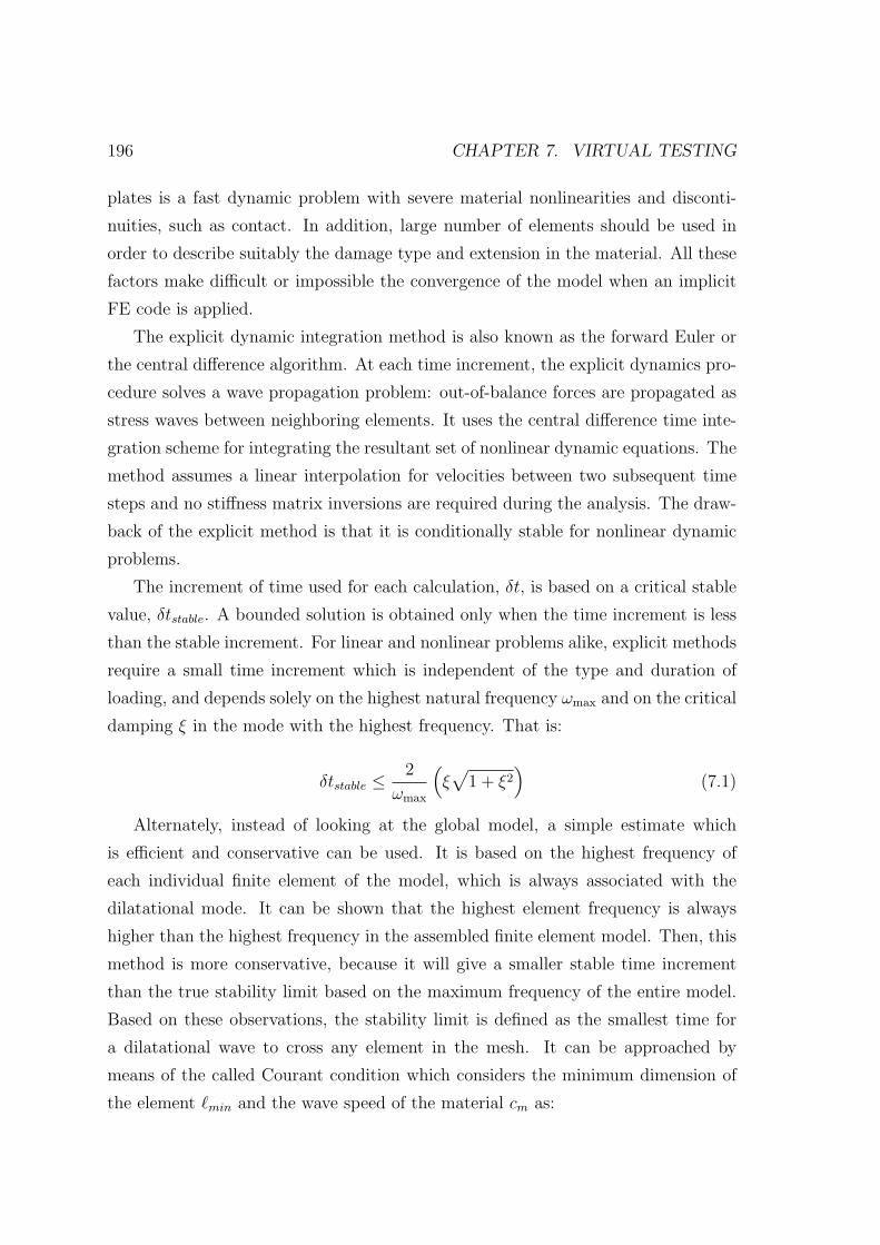
196 CHAPTER 7. VIRTUAL TESTING
plates is a fast dynamic problem with severe material nonlinearities and disconti-
nuities, such as contact. In addition, large number of elements should be used in
order to describe suitably the damage type and extension in the material. All these
factors make difficult or impossible the convergence of the model when an implicit
FE code is applied.
The explicit dynamic integration method is also known as the forward Euler or
the central difference algorithm. At each time increment, the explicit dynamics pro-
cedure solves a wave propagation problem: out-of-balance forces are propagated as
stress waves between neighboring elements. It uses the central difference time inte-
gration scheme for integrating the resultant set of nonlinear dynamic equations. The
method assumes a linear interpolation for velocities between two subsequent time
steps and no stiffness matrix inversions are required during the analysis. The draw-
back of the explicit method is that it is conditionally stable for nonlinear dynamic
problems.
The increment of time used for each calculation, δt, is based on a critical stable
value, δtstable. A bounded solution is obtained only when the time increment is less
than the stable increment. For linear and nonlinear problems alike, explicit methods
require a small time increment which is independent of the type and duration of
loading, and depends solely on the highest natural frequency ωmax and on the critical
damping ξ in the mode with the highest frequency. That is:
δtstable ≤2
ωmax
(ξ√
1 + ξ2)
(7.1)
Alternately, instead of looking at the global model, a simple estimate which
is efficient and conservative can be used. It is based on the highest frequency of
each individual finite element of the model, which is always associated with the
dilatational mode. It can be shown that the highest element frequency is always
higher than the highest frequency in the assembled finite element model. Then, this
method is more conservative, because it will give a smaller stable time increment
than the true stability limit based on the maximum frequency of the entire model.
Based on these observations, the stability limit is defined as the smallest time for
a dilatational wave to cross any element in the mesh. It can be approached by
means of the called Courant condition which considers the minimum dimension of
the element `min and the wave speed of the material cm as:

7.2. DESCRIPTION OF THE FE MODELS 197
δtstable ≤`mincm
(7.2)
where the wave speed is a material property defined as cm =√
Eρ
. E and ρ represent
the bulk stiffness and the density, respectively, of the considered finite element [124,
161].
7.2.2 Plate modeling
Alternatives for plate modeling
The constitutive models for the description of the delamination and the intralaminar
damage mechanisms have been formulated with the aim of simulating the composite
structure at the meso-scale level. Although the initiation and the propagation of
failure inside of each ply occur on the micro-scale, the meso-scale approach is adopted
because the modeling of the entire microstructure is computationally unaffordable.
At this scale level, the interaction of both constitutive models is ensured since they
are used in the same FE model.
In this way, the level of FE discretization considered for a laminated composite
plate is illustrated in Figure 7.1. In the through-the-thickness direction, each ply is
represented by a single layer of 3D solid elements, at which the intralaminar damage
model is assigned. In the case of delamination, the crack planes are known a-priori.
Under impact loading, delamination only occurs between plies with different fiber
orientation. Therefore, cohesive connections described by means of the delamination
model are introduced only in these locations. This simplification goes in favor of
reducing the computational time of the analysis, since in ply clusterings with equal
fiber orientation no cohesive connections are defined.
According to the capabilities offered by the Abaqus/Explicit software, different
alternatives for plate modeling can be considered, as shown in Figure 7.2. Basically,
these alternatives are differentiated as how the cohesive connections are modeled.
For all cases shown in Figure 7.2, the intralaminar damage model is assigned to
the corresponding finite elements by means of the implementation of a user-written
material subroutine, called VUMAT [124].

198 CHAPTER 7. VIRTUAL TESTING
Figure 7.1: Superposition of the finite element discretization with an image of a
laminated composite material (image of the composite material from Olsson [162]).
The case depicted in Figure 7.2.a is the most common way to model the com-
posite plate. It consists of modeling the cohesive connections using solid (non-zero
thickness, he 6= 0) or surface finite elements (zero thickness, he = 0), and the in-plane
size of the mesh of all layers is defined equal, including composite plies and cohesive
type layers. Therefore, the nodes of each layer are shared with the neighboring lay-
ers. In this case, the delamination model can be implemented using a user-written
material subroutine VUMAT (as shown in Chapter 5), or a user-written finite el-
ement subroutine, called VUEL. A drawback of using cohesive elements is that it
makes worse the runtime analysis, because their thickness is small, yielding to small
stable time increments.
(a) (b) (c)
Figure 7.2: Strategies for modeling a laminated composite plate: (a) using cohesive
elements and a regular mesh, (b) using cohesive elements and tie constraints, or
(c) using surface-based cohesive interactions. The variables shown are: h, the plate
thickness; he, the thickness of the cohesive connection; and hp, the thickness of the
ply clustering.

7.2. DESCRIPTION OF THE FE MODELS 199
If non-coincident meshes are used because the mesh of each ply is structured
according to the corresponding fiber orientation (as suggested in Section 6.3 in or-
der to describe properly matrix cracks and thus to reduce the mesh dependency),
or simply because it is desired to use different in-plane mesh sizes for each layer,
the use of Tie Constraints is needed (see Figure 7.2.b). A tie constraint is a ca-
pability of Abaqus/Explicit that provides a simple way to bond surfaces together
permanently, making the translational and rotational motion equal for the pair of
surfaces. However, the use of tie constraints requires additional computational re-
sources and runtime for the pre-processing and analysis phases of the FE model,
often making the acquisition of the virtual solution unaffordable.
Alternately to the case depicted in Figure 7.2.b, it is possible to use a surface-
based cohesive interaction by the implementation of a user-written subroutine type
VUINTER [124] (see Figure 7.2.c). This approach is a quick and easy way to model
cohesive connections, avoiding the need of defining cohesive elements and tie con-
straints, which oppose in improving the runtime of the analysis. However, surface-
based cohesive interactions also can yield to large runtime analysis because contact
algorithms are computationally heavy, especially when the connected meshes are
highly refined. In addition, this type of interaction requires to define one of the con-
nected surfaces (the slave surface), smaller than the other surface which acts as a
reference (master surface), in order to know at any increment of time the surface lo-
cations for the corresponding nodal calculations. Therefore, it supposes that a small
part of the surfaces can not be linked, and if the cohesive connection is subjected
to large relative in-plane sliding, the cohesive connection can yield to inaccurate
results. Finally, another limitation of using a surface-based cohesive interaction is
that the visualization of user state variables of the implemented subroutine for the
post-processing FE phase is not available. Therefore, to plot the virtual extensions
and shapes of the delaminated areas is not possible.
Despite the fact that using in-plane structured meshes oriented with the fiber di-
rection has clear advantages, the solution finally adopted for the plate discretization
is the case depicted in Figure 7.2.a, by using two user-written material subroutines
VUMAT coded with FORTRAN programming language. After several tests using
the different alternatives, the case adopted yields to a well-balanced compromise of
required and available computer resources, capabilities for pre- and post-processing

200 CHAPTER 7. VIRTUAL TESTING
FE phases, as well as the acquisition of suitable results in an acceptable runtime
analysis, which is the fact with more weight.
Type of finite element and dimensions
All layers of the laminated composite plate, including composite plies and cohesive
layers, are modeled by means of 3D hexahedral continuum solid elements with eight
nodes and reduced integration (one integration point), called C3D8R [124].
As noted previously, in the through-the-thickness direction each ply clustering
or cohesive layer is represented by a single layer of solid elements. The thickness
of all cohesive layers is subtracted from the corresponding real plate thickness. In
detail, the thickness of each cohesive layer, he, is defined with 0.01mm. Using
the properties summarized in Table 7.2, the cohesive thickness selected is much
smaller than the maximum value obtained by means of Equation (5.77) in order to
guarantee the correct interlaminar energy dissipation without causing snap-back in
the constitutive response.
With the aim of reducing the CPU analysis time, the in-plane mesh size is vari-
able. A central zone of 60mm×60mm with a refined regular mesh of 0.3mm×0.3mm
is defined (`x× `y), and as from of it and until the plate free edges a biased mesh is
modeled (see Figure 7.3). The elements of the plies located in the central zone
are driven by the intralaminar damage model, whereas the behavior of the re-
maining elements is described by a transversally isotropic elastic material from the
Abaqus/Explicit material library. However, different in-plane regions with different
materials are not considered for the cohesive layers, which are described exclusively
by the delamination damage model.
The reason of using elements with small in-plane sizes in comparison with the
plate dimensions is due to requirements of the damage models for the accurate
prediction of the structure response.
On the one hand, for intralaminar damage elements with a characteristic length
(defined as `∗ =√`x`y) higher than the maximum size `∗max given by Equation
(6.25), the strength of the corresponding damage mode is reduced in order to avoid
snap-back in the constitutive response. These reductions are not adequate in cases
where the results depend strongly on the strengths for damage onset, such as the
prediction of the critical impact load Fd for the sudden loss of the structure stiffness.

7.2. DESCRIPTION OF THE FE MODELS 201
The in-plane dimensions of the intralaminar damage elements are defined small
enough to avoid these strength reductions as can be deduced using the properties
summarized in Table 7.1.
On the other hand, the in-plane size of the cohesive elements should be selected
so the cohesive zone length is suitably split with enough elements (at least with three
or four elements). Accordingly, the in-plane element size selected in the central zone
of the plate is suitable for a proper discretization of the cohesive zone length, as can
be deduced using the properties of Table 7.2 and by means of Equations (5.78) and
(5.79). However, the cohesive description in regions close to the edges of the plate is
deteriorated, but it is not of significance since the delaminations occur mainly into
or near to the central region.
Figure 7.3: In-plane mesh size of the plate.
Definitions to control finite element instabilities
The use of first-order and reduced-integration finite elements can result in a mesh
instability problem, commonly referred to as hourglassing. The hourglassing problem
means that the elements can distort in such a way that the strains calculated at
the integration point are all zero, which, in turn, leads to uncontrolled distortion
of the mesh with no stresses resisting the deformation. Abaqus/Explicit includes
control methods for suppressing hourglassing, where the Enhanced Hourglass Control
approach is the method selected for all simulations.
Moreover, a Distortion Control is used in order to prevent elements from invert-
ing (negative element volumes) or other excessive distorting which are not caused by

202 CHAPTER 7. VIRTUAL TESTING
hourglassing instabilities, rather by the loading conditions and by the level of ma-
terial degradation. This control applies penalty loads when the element is inverted
a predefined proportion of the corresponding original element size.
Additionally, a damping associated with the volumetric straining of the elements,
called Bulk Viscosity, is introduced with the purpose of improving mainly the dy-
namic simulation of the impact tests. A bulk viscosity pressure that varies linearly
with the volumetric strain is defined in order to damp ringing in the highest ele-
ment frequency. Moreover, a pressure that varies quadratically with the volumetric
strain is also introduced with the aim of preventing elements from collapsing un-
der extremely high velocity gradients. The damping coefficients used are the ones
suggested by the FE software, 0.06 and 1.2 for linear and quadratic damping, re-
spectively.
Once the stiffness of a finite element is fully degraded, this element has no con-
tribution to the stiffness of the model, but can reduce the stable time increment
during the simulation. Abaqus/Explicit offers the choice to remove these elements
from the mesh. It is selected that a cohesive element is removed when its scalar
damage variable d reaches the value of 0.99. However, the criterion for deleting
ply elements is more complex since a directional damage model describes their con-
stitutive behavior. In the simulations proposed here, these elements are removed
when the longitudinal damage variable d1 reaches 0.999, i.e. fiber breakage. As can
be seen, the elements are removed before the damage variables reach the unity in
order to avoid possible sudden element distortions because of the absence of residual
stiffness. Accordingly, the transverse and shear damage variables d2, d3, d4, d5 and
d6 are also limited to a maximum value of 0.99.
Mainly, the cohesive elements will determine the stable time increment of the
whole model due to their small thickness, as it can be deduced from Equation (7.2).
The computational efficiency of the simulations is improved by scaling the mass of
these elements by means of the Variable Mass Scaling capability of Abaqus/Explicit.
In detail, it is selected to scale the masses of only the cohesive elements whose stable
time increment is less than a predefined value. Such definitions are selected taking
care of never increase significantly the overall mass of the plate.
In order to verify if excessive use of the solutions mentioned for decreasing nu-
merical difficulties (hourglass control, the distortion control, the viscosity damping,

7.2. DESCRIPTION OF THE FE MODELS 203
and mass scaling) occurs during the simulations, an engineering judgment based on
the lecture of the corresponding energy variables should be performed. Typically,
the energy generated by each one of these solutions must be less than 1% of the
internal energy of the system.
Material properties
The material properties of the AS4/8552 carbon-epoxy unidirectional pre-preg are
summarized in Table 7.1. These properties are inputs to fed on the intralaminar
damage model. Some of the properties were obtained by testing specimens man-
ufactured with the same pre-preg roll of the specimens used for the experimental
impact and CAI tests. The properties which were not obtained experimentally, are
extracted from the literature.
Table 7.1: Hexply AS4/8552 properties. The properties pointed out with (∗) are
extracted from [97].
Density [kg/mm3] 1590× 10−9
Elastic properties E1 = 128.00GPa; E2 = 7.63GPa;
E6 = G12 = 4.36GPa;
ν12 = 0.35; ν23 = 0.45
Strength [MPa] X1+ = XT = 2300.0; X1− = XC = 1531.0∗;
X2+ = YT = 26.0; X2− = YC = 199.8∗;
X6 = SL = 78.4
Fracture toughness [N/mm] G1+ = 81.5∗; G1− = 106.3∗; G2+ = 0.28∗; G6 = 0.79∗
Other definitions required by the intralaminar damage model are: XPO = 0.1XT
(pull-out strength), GL1+ = 0.2G1+ (energy dissipated at linear softening), GE1+ =
G1+ − GL1+ (energy dissipated at exponential softening), G2− = G6/ cos(α0), and
α0 = 53. Since the differences of temperature and moisture are not considered
in the simulations, the definition of the thermal coefficients and of the hygroscopic
expansion are not required. In addition, the transverse tensile strength YT and
the in-plane shear strength SL are adjusted in order to consider the in-situ effect

204 CHAPTER 7. VIRTUAL TESTING
according to the equations shown in Chapter 6. For the calculation of the in-situ
in-plane shear strength, it is taken ς = 2.98× 10⁻⁸.
On the other hand, the properties used for the interlaminar damage model are
summarized in Table 7.2.
Table 7.2: Interface properties.
Density [kg/mm3] 1590× 10−9
Elastic properties E = 7.63GPa; ν = 0.45
Mode I strength [MPa] τ o3 = YT = 26.0
Fracture toughness [N/mm] GIc = G2+ = 0.28; GIIc = G6 = 0.79
Other definitions required to fed on the interlaminar damage model are: mode
II interlaminar shear strength, τ o1 = τ o3
√GIIcGIc
[13]; and the parameter of the least-
square fit of the mixed-mode fracture toughness values, η = 1.45 [97].
7.2.3 Virtual test set-up
Drop-weight impact tests
According to the impact test set-up used for the real tests shown in Figure 3.1, the
virtual models should reproduce the same conditions but in the most simplified way
in order to avoid unnecessary computer time consuming.
In Figure 7.4 is shown the assembly of the different components considered for
the simulation of the impact test. The fixture base support and the hemispherical
impactor are defined as a rigid bodies since they are stiff steel parts whose stresses
and strains are not of interest. In detail, the impactor is modeled by a lumped mass
element and the fixture base by 3D rigid elements with four nodes, called R3D4. If
domain parallelization is used for the analysis calculation, the fixture base should
be meshed with enough elements in order to split it in enough element sets, just
as much as the number of domains. The maximum element length selected for the
fixture base mesh is of 5mm.
The motion of a rigid body is governed by the motion of a single reference
point at which the boundary conditions, initial conditions and physical parameters
are defined. Certainly, the fixture base is defined with all the degree of freedom

7.2. DESCRIPTION OF THE FE MODELS 205
constrained. The impactor is also defined with all the degree of freedom fixed, in
exception of the out-of-plane displacement. In order to capture the effect of the im-
pactor drop, the impactor is modeled just before of the impact position by specifying
an initial impact velocity consistent with the height of free fall. In addition, a con-
centrated load is defined on the impactor to describe the weight load, although its
effect is practically insignificant since the impact forces reaches much higher values.
Figure 7.4: Set-up of the virtual impact tests.
The four rubber-tipped clamps which restrain the specimen over the fixture base
are modeled by means of the Distributed Coupling Constraint capability. These
constraints couple the motion of a group of nodes to the motion of a master node.
Therefore, at each master node is defined an instantaneous out-of-plane load of
3000N, which is uniform distributed to the corresponding affected set of nodes lo-
cated on the top plate surface. The influence radius to select the corresponding set
of coupled nodes is of 7mm.
On the other hand, contact constraints are required in order to describe the
contact between the impactor and the top face surface of the plate, and also the
back face surface of the plate with the fixture base. The contact approach used is

206 CHAPTER 7. VIRTUAL TESTING
the General Contact algorithm of Abaqus/Explicit, which defines a linear pressure-
overclosure relationship between the contacting surfaces, where the contact stiffness
is chosen automatically by the software, and there is not limit to the magnitude
of the contact pressure that can be transmitted. In addition, the Coulomb friction
model which relates the maximum allowable frictional shear stress across an interface
τmax to the normal contact pressure between the contacting bodies P , τmax = µP , is
defined. In detail, the friction coefficient for contacts between a steel material and
a composite material is considered as µ = 0.3.
As it has been noted in previous section, once the finite elements of the plate
are completely degraded, they are removed from the mesh in order to improve the
computation efficiency. Due to this fact, new internal element faces can be subjected
to contact with the impactor, or even with the neighboring elements. Therefore,
contact constraints should be defined for these possible interactions.
Since in the proposed impact simulations the perforation does not occur, it is
enough to consider that the impactor can take contact with the first three top
surfaces of the element sets which describe the first three composite plies.
In addition, the internal faces of the elements located in the regular zone depicted
in Figure 7.3 are modeled in such a way that could take contact themselves during the
simulation. The friction coefficient in delaminated interfaces varies from 0.2 for 0/0
interfaces (with sliding in the longitudinal direction), to 0.8 for 90/90 interfaces
(with sliding in the transversal direction) [163]. An average friction coefficient of 0.5
is applied between element faces, as suggested in [97].
It should be noted that any contact definition increases the required computer
memory, as well as it makes worse the runtime analysis of the model, since the
relative displacement between contact surfaces is checked periodically during the
simulation. Therefore, the fewer contact definitions, faster the simulation will reach
the solution.
CAI tests
Once the simulation of the impact test is finished, the CAI test is subsequently
carried out. Therefore, the post-impact structure state should be imported and the
new boundary conditions which reproduce the CAI test should be defined. In detail,
the damaged plate is imported by means of the Restart and Import capabilities of

7.2. DESCRIPTION OF THE FE MODELS 207
Abaqus/Explicit, and the boundary conditions are illustrated in Figure 7.5. These
boundary conditions are simply modeled by constraining the corresponding degree
of freedom of the nodes located at the sites pointed out.
Although the CAI test is essentially quasi-static, it will be simulated by means
of the dynamic FE code Abaqus/Explicit. The reason is due to the fact that high
material and geometrical non-linearities occur, yielding to severe convergence diffi-
culties if an implicit FE code is used. Accordingly, a displacement loading is applied
with sufficiently slowness at one of the short edges of the plate (see Figure 7.5), so
the kinetic energy is kept despicable against the internal energy of the system.
Figure 7.5: Boundary conditions of the CAI test.
7.2.4 Energy balance
The evolution of the energy variables is a valuable data to know the events that can
occur during the numerical impact simulation, and then to assess if the simulation
is yielding to an appropriate response. Mainly, these events are the onset and the
progression of each damage mechanism that the composite material can suffer, and
also, the use of the solutions considered for the proper working of the numerical
models, such as the generation of artificial energy for hourglassing prevention.
For the virtual tests considered herein, the energy balance equation can be writ-
ten as:
ET = EK + EI + EF + EV −WE −WC −WMS (7.3)

208 CHAPTER 7. VIRTUAL TESTING
where ET is the total energy of the system, EK is the kinetic energy, EI is the
internal energy, EF is the frictional dissipation energy, EV is the energy dissipated
by bulk viscosity damping, WE is the work of the external forces, WC is the work
done by contact penalties, and WMS is the work done in propelling mass added in
mass scaling. The internal energy can be split in the following terms:
EI = EE + EH + EDC + EDm + EDf + EDd (7.4)
where EE is the recoverable strain energy (elastic energy), EH is the energy gen-
erated to prevent hourglassing, and EDC is energy dissipated by distortion control.
The terms EDm, EDf , and EDd are the energy dissipated by matrix damage, by fiber
damage, and by delamination, respectively.
Most of the energy terms can be requested for the entire model or for specific
element sets of the model.
7.3 Results of the virtual tests and comparison
with experimental data
At following, the results of the impact test and CAI test simulations are presented
and compared with the experimental data shown in Chapter 4.
The simulations have been performed using multiple processors on separate ma-
chines, i.e. cluster. Abaqus/Explicit automatically breaks up the FE model into
domains and assigns each domain to a processor, so the analysis is carried out in-
dependently in each domain. Since the domains share common boundaries, the
information is passed between the domains at each increment via the MPI interface
mode (Message Passing Interface) [124]. At the end of the analysis, the individual
files are merged automatically.
In detail, the FE models are parallelized in a cluster composed by a group of six
linked computers, each one with 8GB RAM and four processors (24 CPUs). The
whole runtime analysis of the impact and CAI tests has ranged between twelve and
fifteen days, depending on the plate stacking sequence. The simulations are heavy
due to the large number of composite plies and cohesive interfaces (each layer is
modeled with an element), the small in-plane sizes of the elements, and the large

7.3. VIRTUAL RESULTS AND COMPARISON WITH EXPERIMENTS 209
number of contact definitions. These factors yield to small time increments (of the
order of 1e-9s), where each one requires fairly long time of analysis. In addition, the
impact events considered are long in time (of the order of 5e-3s), so large amount
of increments are required to complete the simulation.
It should be noted that not all the impact configurations tested are performed
virtually, because of limitations in computer memory resources for the pre-process
and analysis FE phases. Only, some cases of the ply clustering study are considered.
The unresolved impact configurations are proposed as future works.
Laminate L04
Figures 7.6, 7.7 and 7.8 show the comparisons between the experimental and the
numerical evolutions of the impact force of the laminate L04 for 38.6J, 28.6J and
19.3J, respectively. As can be observed, the whole profiles and the contact times are
quite well predicted, whereas the damage thresholds Fd are clearly over-predicted.
Moreover, in contrast with the experimental results, it is detected that the numerical
values of Fd are not kept constant by changing the impact velocity.
0 1 2 3 4 5 60
2000
4000
6000
8000
10000
12000
14000
Fd,e
Fd,n
Time [ms]
Forc
e [N
]
ExperimentalNumerical
Figure 7.6: Experimental and numerical impact force histories of the laminate L04
for 38.6J.
Several differentiable simulations have been carried out in order to explain the
fact that generates the over-prediction of Fd. Firstly, the mesh of the outer ply at
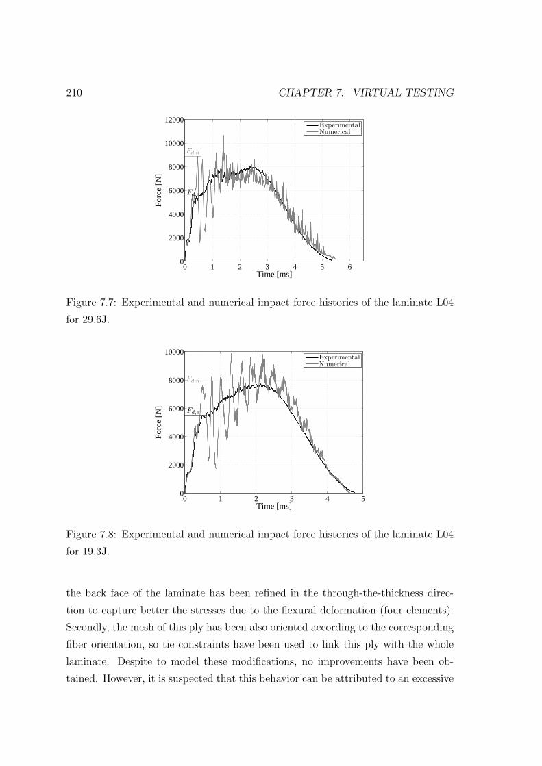
210 CHAPTER 7. VIRTUAL TESTING
0 1 2 3 4 5 60
2000
4000
6000
8000
10000
12000
Fd,e
Fd,n
Time [ms]
Forc
e [N
]
ExperimentalNumerical
Figure 7.7: Experimental and numerical impact force histories of the laminate L04
for 29.6J.
0 1 2 3 4 50
2000
4000
6000
8000
10000
Fd,e
Fd,n
Time [ms]
Forc
e [N
]
ExperimentalNumerical
Figure 7.8: Experimental and numerical impact force histories of the laminate L04
for 19.3J.
the back face of the laminate has been refined in the through-the-thickness direc-
tion to capture better the stresses due to the flexural deformation (four elements).
Secondly, the mesh of this ply has been also oriented according to the corresponding
fiber orientation, so tie constraints have been used to link this ply with the whole
laminate. Despite to model these modifications, no improvements have been ob-
tained. However, it is suspected that this behavior can be attributed to an excessive
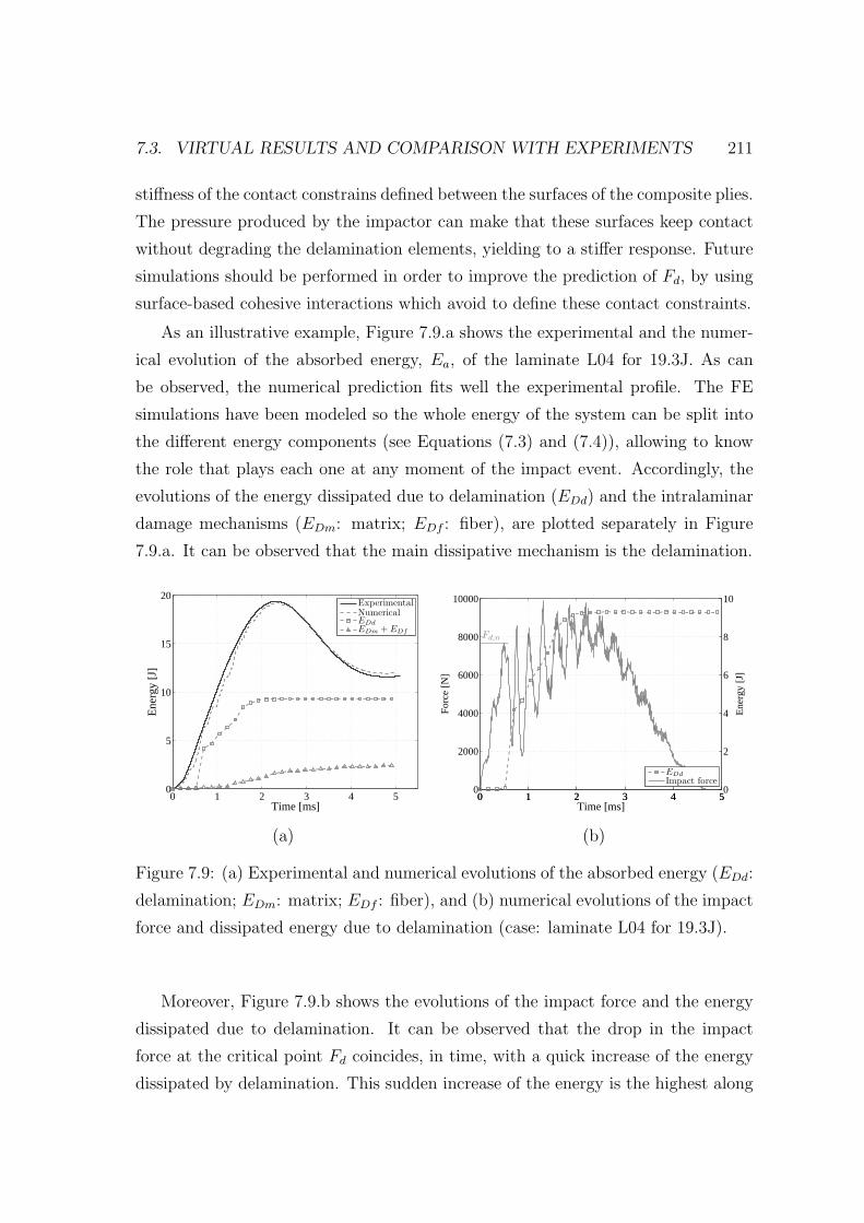
7.3. VIRTUAL RESULTS AND COMPARISON WITH EXPERIMENTS 211
stiffness of the contact constrains defined between the surfaces of the composite plies.
The pressure produced by the impactor can make that these surfaces keep contact
without degrading the delamination elements, yielding to a stiffer response. Future
simulations should be performed in order to improve the prediction of Fd, by using
surface-based cohesive interactions which avoid to define these contact constraints.
As an illustrative example, Figure 7.9.a shows the experimental and the numer-
ical evolution of the absorbed energy, Ea, of the laminate L04 for 19.3J. As can
be observed, the numerical prediction fits well the experimental profile. The FE
simulations have been modeled so the whole energy of the system can be split into
the different energy components (see Equations (7.3) and (7.4)), allowing to know
the role that plays each one at any moment of the impact event. Accordingly, the
evolutions of the energy dissipated due to delamination (EDd) and the intralaminar
damage mechanisms (EDm: matrix; EDf : fiber), are plotted separately in Figure
7.9.a. It can be observed that the main dissipative mechanism is the delamination.
0 1 2 3 4 50
5
10
15
20
Time [ms]
Ene
rgy
[J]
ExperimentalNumericalEDdEDm + EDf
0 1 2 3 4 50
2000
4000
6000
8000
10000
Time [ms]
Forc
e [N
]
Fd,n
0 1 2 3 4 50
2
4
6
8
10
Ene
rgy
[J]
EDdImpact force
(a) (b)
Figure 7.9: (a) Experimental and numerical evolutions of the absorbed energy (EDd:
delamination; EDm: matrix; EDf : fiber), and (b) numerical evolutions of the impact
force and dissipated energy due to delamination (case: laminate L04 for 19.3J).
Moreover, Figure 7.9.b shows the evolutions of the impact force and the energy
dissipated due to delamination. It can be observed that the drop in the impact
force at the critical point Fd coincides, in time, with a quick increase of the energy
dissipated by delamination. This sudden increase of the energy is the highest along

212 CHAPTER 7. VIRTUAL TESTING
the chart. This result corroborates with the comments written in previous chapters,
where it is assumed that the first drop in the impact force is mainly due to a large
growth of delaminations when the structure is loaded under a low-velocity impact.
Figure 7.10 shows the predicted delamination area at two different contact times:
(a) ti = 0.4ms (just before to reach Fd), and (b) ti = 0.8ms (just after the first
drop of the impact force). The field variable plotted corresponds to the scalar
damage variable of all the interface elements, so a translucency is applied in order
to visualize all the interfaces. These projections are such as the images that can be
obtained by C-scan inspections. It can be observed a large and quick increase of the
delaminations between these two instants of time, as deduced previously in Figure
7.9.b.
(a) (b)
Figure 7.10: Projected delaminated area for impact times, (a) ti = 0.4ms and (b)
ti = 0.8ms.
According to the numerical predictions, a certain number of delaminations prop-
agate simultaneously at the critical point Fd. Therefore, the development of ana-
lytical damage thresholds based on the assumption that a single delamination can
generate a drop in the impact force history, is not fully clear.
In a similar way as the procedure used by Davies et al. [69, 85] to formulate
an analytical threshold Fd based on the propagation of a single circular mid-plane
delamination (F statd1 , see Equations (2.112) and (2.113)), a new criterion can be de-
veloped assuming that n∗d delaminations can grow. These delaminations are counted
from the back face of the plate, and generate n∗d sub-laminates with a thickness equal
to the clustering thickness hp (see Figure 7.11). This approach is interesting for cases

7.3. VIRTUAL RESULTS AND COMPARISON WITH EXPERIMENTS 213
which suffer the largest delaminations at the deeper interfaces of the laminate (i.e.
close to the back face of the laminate), often yielding to a wide pine tree damage
pattern (see Figure 2.11.a). The resulting equation deduced by means of LEFM is
defined as:
F statdbf = π
√8EGIIc
3 (1− ν2)
(− 1
h3+
1
(h− n∗dhp)3 + n∗dh3p
)− 12
(7.5)
where GIIc is the fracture toughness in pure mode II, E and ν are respectively the
homogenized in-plane elastic modulus and Poisson ratio of the plate, h is the plate
thickness, hp is the clustering thickness, and n∗d is the number of delaminations
considered.
Figure 7.11: Example of back face delaminations.
The threshold F statdbf does not depend on the initial crack length of the n∗d de-
laminations, so it can be interpreted as a criterion for delamination onset. As can
be checked, increasing the value of n∗d, the load required to grow the delaminations
decreases since the flexural stiffness of the plate is reduced. Table 7.3 summarizes
the values of F statdbf for laminates L02, L03, and L04, for different number of sub-
laminates. The values of F statdbf written in bold are the ones which are closer to the
experimental values.
Figure 7.12 shows the comparisons between the numerical and the C-scan pro-
jected delamination areas at the end of the impact event of the laminate L04 for
each impact energy. In a general point of view, the predictions agree with the ex-
perimental data. It should be noted that the predicted results are influenced by the
in-plane mesh refinement. When a delamination reaches the rough mesh (see Figure
7.3), the growth of the delamination can be restrained because the FE discretization
of the cohesive zone length is not enough.

214 CHAPTER 7. VIRTUAL TESTING
Table 7.3: Values of F statdbf to generate n∗d sub-laminates counted from the back face
of the plate (laminates L02, L03 and L04).
LaminatePly thickness Number of Experimental threshold Analytical threshold
hp [mm] interfaces nd load Fd,e [kN] load F statdbf [kN]
L02 0.181 30 9.94
n∗d = 10 10.43
n∗d = 11 9.44
n∗d = 12 8.54
L03 0.363 14 7.60
n∗d = 6 8.57
n∗d = 7 7.02
n∗d = 8 5.73
L04 0.725 6 5.50
n∗d = 3 8.67
n∗d = 4 5.80
n∗d = 5 3.88
Ei = 38.6J Ei = 28.6J Ei = 19.3J
Figure 7.12: Projected delamination areas of the laminate L04 for each impact
energy (experimental: black line; numerical: dashed gray line).
Figure 7.13 shows an example of through-the-thickness cut views of the plate at
the impact site (case: laminate L04 for 19.3J). The variable plotted corresponds to
the transverse damage variable d2 (matrix cracking) at contact time ti = 2.0ms.
Related to the CAI tests, Table 7.4 summarizes the predictions of the post-impact
residual compressive load Ffc and the compressive displacement at failure of the
laminate L04 for each impact energy. As can be observed, the values of the residual
compressive strengths are well predicted, whereas the compressive displacements at
the failure point are fairly under-predicted.
Taking as an example the CAI test simulation of the laminate L04 impacted with

7.3. VIRTUAL RESULTS AND COMPARISON WITH EXPERIMENTS 215
(a) x = 70mm:
(b) x = 75mm:
(c) x = 80mm:
Figure 7.13: Through-the-thickness views (cut plane: y − z), of matrix cracking
distribution at the impact site (x, y) = (75, 50)mm of the laminate L04, impacted
with 19.3J and at contact time ti = 2.0ms.
Table 7.4: Predictions of the post-impact residual compressive load and the com-
pressive displacement of the laminate L04.
Impact energy [J]Strength Ffc [kN] Displacement ufc [mm]
Experimental Numerical Experimental Numerical
38.6 98 89 1.42 0.5
28.6 103 92 1.37 0.5
19.3 105 107 1.45 0.8
19.3J, in Figure 7.14 are plotted the evolutions of the dissipated energies and the
compression load as a function of the compression displacement. The initial values
of these energies correspond to the energies dissipated at the end of the impact test.
It can be observed that practically the trend of the energies is constant until the
maximum strength is reached. At this point, the energies dissipated due to the
delamination and the intralaminar damage mechanisms increase. The collapse of
the plate is triggered by fiber failure which, in turn, triggers matrix cracking and
delamination.
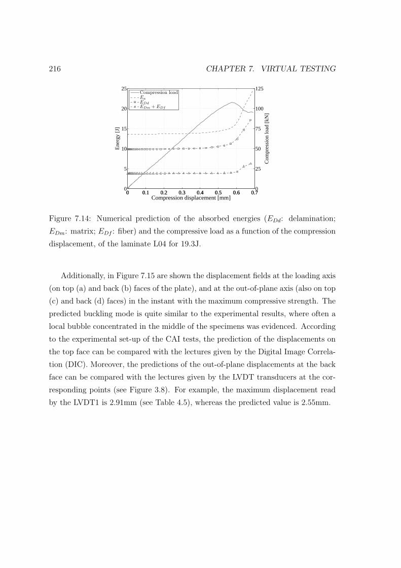
216 CHAPTER 7. VIRTUAL TESTING
0 0.1 0.2 0.3 0.4 0.5 0.6 0.70
5
10
15
20
25
Ene
rgy
[J]
Compression displacement [mm]
0 0.1 0.2 0.3 0.4 0.5 0.6 0.70
25
50
75
100
125
Com
pres
sion
load
[kN
]
Compression loadEaEDdEDm + EDf
Figure 7.14: Numerical prediction of the absorbed energies (EDd: delamination;
EDm: matrix; EDf : fiber) and the compressive load as a function of the compression
displacement, of the laminate L04 for 19.3J.
Additionally, in Figure 7.15 are shown the displacement fields at the loading axis
(on top (a) and back (b) faces of the plate), and at the out-of-plane axis (also on top
(c) and back (d) faces) in the instant with the maximum compressive strength. The
predicted buckling mode is quite similar to the experimental results, where often a
local bubble concentrated in the middle of the specimens was evidenced. According
to the experimental set-up of the CAI tests, the prediction of the displacements on
the top face can be compared with the lectures given by the Digital Image Correla-
tion (DIC). Moreover, the predictions of the out-of-plane displacements at the back
face can be compared with the lectures given by the LVDT transducers at the cor-
responding points (see Figure 3.8). For example, the maximum displacement read
by the LVDT1 is 2.91mm (see Table 4.5), whereas the predicted value is 2.55mm.

7.3. VIRTUAL RESULTS AND COMPARISON WITH EXPERIMENTS 217
(a) (b)
(c) (d)
Figure 7.15: (a) Top face and (b) back face predicted displacement field at the
loading axis direction; (c) top face and (d) back face out-of-plane displacement field
(case: laminate L04 for 19.3J).
Laminate L03
Figures 7.16 and 7.17 show the comparisons between the experimental and the nu-
merical evolutions of the impact force of the laminate L03 for 28.6J and 19.3J, re-
spectively. In contrast with the simulations of the laminate L04, the whole profiles
are not well predicted, whereas the contact times are still more or less in agreement
with the experimental results. The damage thresholds Fd are again over-predicted,
even with more offset than in the simulations of the laminate L04. This result can
be related with the fact that more contact constraints are defined for laminate L03,
because it has more interfaces.
On the other hand, Figure 7.18.a shows the experimental and the numerical
evolutions of the absorbed energy, and the components of the dissipated energy

218 CHAPTER 7. VIRTUAL TESTING
0 1 2 3 4 50
2000
4000
6000
8000
10000
12000
14000
16000
Fd
Fd
Time [ms]
Forc
e [N
]
ExperimentalNumerical
Figure 7.16: Experimental and numerical impact force histories of the laminate L03
for 29.6J.
0 1 2 3 4 50
2000
4000
6000
8000
10000
12000
14000
16000
Fd
Fd
Time [ms]
Forc
e [N
]
ExperimentalNumerical
Figure 7.17: Experimental and numerical impact force histories of the laminate L03
for 19.3J.
(delamination and intralaminar damages), of the laminate L03 for 19.3J. As can be
observed, the numerical result over-predicts significantly the experimental profile.
In addition, Figure 7.18.b shows the evolutions of the impact force and the energy
dissipated due to delamination. According to the simulations, the main dissipative
mechanism in first drop of the impact force is again the delamination.
Figure 7.19 shows the comparisons between the numerical and the C-scan pro-

7.3. VIRTUAL RESULTS AND COMPARISON WITH EXPERIMENTS 219
0 1 2 3 40
5
10
15
20
25
Time [ms]
Ene
rgy
[J]
ExperimentalNumericalEDdEDm + EDf
0 1 2 3 4 50
4000
8000
12000
16000
Time [ms]
Forc
e [N
]
Fd,n
0 1 2 3 4 50
5
10
15
20
25
Ene
rgy
[J]
EDdImpact force
(a) (b)
Figure 7.18: (a) Experimental and numerical evolutions of the absorbed energy
(EDd: delamination; EDm: matrix; EDf : fiber), and (b) numerical evolutions of
the impact force and dissipated energy due to delamination (case: laminate L03 for
19.3J).
jected delamination areas at the end of the impact event of the laminate L03 for
the impact energies 28.6J and 19.3J. Clearly, the sizes are over-predicted, which
corroborates the result plotted previously in Figure 7.18.a.
Ei = 28.6J Ei = 19.3J
Figure 7.19: Projected delamination areas of the laminate L03 for each impact
energy (experimental: black line; numerical: dashed gray line).
Obviously, since the amount of impact damage is over-predicted, the post-impact
residual strength is under-predicted. The compression strengths and compression
displacements obtained are summarized in Table 7.5.
Taking as an example the CAI test simulation of the laminate L03 impacted with
19.3J, in Figure 7.20 are plotted the evolutions of the dissipated energies and the

220 CHAPTER 7. VIRTUAL TESTING
Table 7.5: Predictions of the post-impact residual compressive load and the com-
pressive displacement of the laminate L03.
Impact energy [J]Strength Ffc [kN] Displacement ufc [mm]
Experimental Numerical Experimental Numerical
28.6 100 120 1.32 0.6
19.3 134 124 1.6 0.6
compression load as a function of the compression displacement. As occurred with
laminate L04, the energies dissipated due to the delamination and the intralaminar
are constant until the maximum strength is reached. On the other hand, in Figure
7.21 are shown the displacement fields at the loading axis (on top (a) and back (b)
faces of the plate), and at the out-of-plane axis (also on top (c) and back (d) faces) in
the instant with the maximum compressive strength. Again, a local bubble appears
on the back-face of the plate.
0 0.2 0.4 0.6 0.80
5
10
15
20
25
30
35
Ene
rgy
[J]
Compression displacement [mm]
0 0.2 0.4 0.6 0.80
20
40
60
80
100
120
140
Com
pres
sion
load
[kN
]
Compression loadEaEDdEDm + EDf
Figure 7.20: Numerical prediction of the absorbed energies (EDd: delamination;
EDm: matrix; EDf : fiber) and the compressive load as a function of the compression
displacement, of the laminate L03 for 19.3J.

7.3. VIRTUAL RESULTS AND COMPARISON WITH EXPERIMENTS 221
(a) (b)
(c) (d)
Figure 7.21: (a) Top face and (b) back face predicted displacement field at the
loading axis direction; (c) top face and (d) back face out-of-plane displacement field
(case: laminate L03 for 19.3J).

222 CHAPTER 7. VIRTUAL TESTING

Chapter 8
Conclusions and future work
8.1 Conclusions
The present thesis covers a wide range of analysis of the low-velocity and large mass
impact events on monolithic, flat, rectangular, polymer-based laminated composite
plates with conventional stacking sequences. Keeping in mind that the main goal
of this work is the prediction of the residual compressive strength of an impacted
specimen coupon, a set of different tasks are performed in order to provide suitable
tools to analyze the problem. In this sense, the topics which are addressed in this
thesis are: the analytical description of the impact, the design and the realization
of an experimental test plan, the formulation and implementation of constitutive
models for the description of the composite material behavior, and the assessment
of the performance of FE virtual tests where the constitutive models are used. In the
following points, the main contributions and conclusions of this thesis are described.
8.1.1 Analytical impact description
Due to the simplicity of the geometry of the structure considered, the development
of analytical models for the description of the impact event can be developed with
sufficient accuracy. In this way, a detailed literature review of the analytical de-
scription is carried out in Chapter 2 and in the related Appendix A. The analytical
models offer preliminary information for a given impact configuration, allowing the
understanding of the effects of each parameter that influence the impact response.
223

224 CHAPTER 8. CONCLUSIONS AND FUTURE WORK
Thus, the tools reviewed are used to acquire an initial knowledge of the problem,
and also for planning the experimental test campaign.
The literature survey is focused on the models which describe the elastic response
of the impact event. Different types of models are analyzed, covering the complete
analytical models which fully describe the dynamic behavior of the problem, and
the simplified models which describe a particular extreme impact behavior. Accord-
ingly, the basis of any impact model, which are the contact laws and the governing
equations of the plate and the impactor, are analyzed in detail. Additionally, the
dimensionless frameworks which reduce suitably the number of influencing impact
parameters in a more manageable dimensionless key parameters are also described.
Although the analytical description performed is focused on laboratory coupons,
most of the concepts reviewed can be used for other structures with more complex
shapes.
The variable used to bridge the elastic stress/strain analysis and the onset of
damage is the maximum impact load, which is compared with a damage threshold
allowable. Damage occurs if the predicted maximum load is greater than a well-
defined threshold for the corresponding dynamic response type.
Taking into account that under low-velocity impact loading the main and the
most dangerous damage mechanism is the delamination, which reduces severely the
residual compressive strength of the structure, the analytical damage analysis is
particularized on the delamination onset. This failure mode can be detected as
a first drop in the lecture of the impact force history. A new damage threshold
which predicts delamination at the deepest interface of the plate is developed. It
is assumed that this delamination is triggered by a vertical matrix crack located at
the outer ply of the back face of the plate.
8.1.2 Experimental test plan
The sequential experimental tasks which are carried out in order to analyze labo-
ratory coupons are: definition of the impact tests, manufacturing of the specimens,
C-scan inspections for the detection of manufacturing flaws, instrumented drop-
weight impact tests, dent-depth measurements, C-scan inspections to detect the
BVID, and finally, instrumented CAI tests.
The selection of the impact tests is done using some of the analytical tools

8.1. CONCLUSIONS 225
previously described and taking as a reference the American Standard Test Method
for drop-weight impact on laminated composite plates [59]. Modifying some of the
standard parameters, three main studies are proposed: effect of the ply thickness
(clustering), effect of the mismatch angles of the plies, and effect of the laminate
thickness. In addition, the effect of the impact velocity, and the effect of changing
the impact velocity and the impactor mass but keeping constant the impact energy,
are also analyzed inside of the main proposed studies. Among the proposed studies,
the most innovative is the analysis of the ply thickness effect on the impact response.
For each impact study, the appearance of the first large damage is analyzed in detail.
The goal of these studies is not to obtain an improved damage resistant or damage
tolerant structure, rather to obtain a wide range of different experimental data that
can be subsequently used to validate the numerical simulations of the impact and
the CAI tests.
The main conclusions of the experimental results and their comparison with
analytical models are listed below:
Effect of the impact velocity
• The threshold load, Fd, remains constant in front of changes of the impact
velocity.
• Increasing the impact velocity, the slope of the elastic regime is increased, as
predicted by means of the analytical impact models. Accordingly, the pre-
dicted maximum elastic impact force increases, indicating that more damage
is created.
• Increasing the impact velocity, the response is extended in time because the
plate develops more damage. Accordingly, the post-impact residual compres-
sive strength is reduced.
Effect of changing the impactor mass and the velocity
• The threshold load, Fd, remains constant in front of changes of the impactor
mass and velocity, but keeping constant the impact energy.
• Increasing the impactor mass, the response is more quasi-static, which means
226 CHAPTER 8. CONCLUSIONS AND FUTURE WORK
that the response is slowed down. This behavior can also be predicted by
means of the impact characterization diagram and the complete analytical
impact models.
• Given a stacking sequence, the dissipated energy or the damage developed is
the same between impacts with equal impact energy. In addition, the residual
compressive strength remains constant under the same impact energy level.
This result agrees with some of the guidelines provided by the aeronautical
industry for a drop-weight impact test, where the energy is specified, and the
impactor mass and the velocity can be selected freely by the engineer.
Effect of ply thickness (clustering)
• If the ply clustering is increased, under equal impact conditions the values of
Fd and Fmax are reduced.
• Increasing the ply clustering, the changes in the stiffness during the impact are
more progressive and smooth when compared with laminates with thin plies.
This result implies difficulties in the detection of Fd for laminates with thick
plies.
• The response is elongated by increasing the ply clustering of the laminate. This
result indicates that more damage develops for laminates with thick plies. Ac-
cordingly, by reducing the number of interfaces available for delamination, the
resulting projected delamination area is increased. Therefore, ply clustering
results in a lower damage resistance of a composite structure.
• Increasing the ply clustering, the indentation is increased.
• The free growth of the delaminations can be affected by the finite in-plane
dimensions of the plates. In other words, the growth of the delaminations could
be braked by the clamping system. This effect occurs basically in laminates
with thick plies.
• The trend of the proposed analytical thresholds for delamination are in agree-
ment with the experimental points for all laminate types. However, the ana-
lytical values under-predict the real values. This offset can be due to scattering

8.1. CONCLUSIONS 227
of the material properties or to the assumptions considered in the formulation
of the damage threshold, e.g. strain rate effects are neglected. Further testing
is required to verify these arguments, especially with critical impact energies
which generate maximum impact forces similar to the damage threshold loads.
• The damage tolerance, quantified using the residual compressive load, is not
affected by increasing the ply thickness, because all presented laminate types
have shown similar values of compressive loads at each impact energy.
Effect of ply mismatch angle at interfaces
• The analytical prediction of Fd for the selected cross-ply laminate has been in
agreement with the experimental result, although an offset also has appeared.
• The mismatch angle of the interfaces for delamination has not presented a clear
effect on the damage resistance and on the damage tolerance. This result can
be due to the fact that the plate thicknesses of the selected laminates for this
study are slightly different.
Effect of the laminate thickness
• Increasing the laminate thickness, the response is faster and the drop in the
impact force from point Fd increases. For the thinner laminate tested, the
profiles of the impact force are smooth and do not present a clear first drop
on the impact force. This result could mean that a sudden loss of stiffness
from the point Fd does not occur, or the matrix and delamination damage
that appear do not change the response of the impact, rather it is affected by
progressive fiber breakage. This last argument can be related to the membrane
effects.
• The predictions of the threshold load Fd for the different laminates considered
have been in agreement except for the thinner laminate, i.e. L01. This result
can be attributed to different causes: the membrane effects, the possibility
that really the delaminations can not be detected in the force histories, or the
fact that simply a sudden large delamination does not occur and rather the
delaminations grow progressively.

228 CHAPTER 8. CONCLUSIONS AND FUTURE WORK
• Increasing the laminate thickness, the damage resistance is improved since
the energy dissipated is lower than for thin laminates. Likewise, the damage
tolerance is improved. However, the resulting structures are heavier and more
expensive.
Usefulness of the analytical impact models and analytical thresholds
• With the studies presented, it has been demonstrated that the analytical im-
pact models for the prediction of the elastic response are a powerful tool: to
define a suitable test matrix of specimens, to obtain a qualitative understand-
ing of the effects of the governing parameters on the impact response, and to
interpret the experimental results obtained.
• The analytical impact models are completed with the analytical thresholds for
the prediction of the damage mechanisms that can occur in a laminated com-
posite plate under low-velocity impact loading. For low-velocity impacts, the
most critical damage is the delamination. In general, it has been shown that
the damage thresholds for delamination follow the trends of the experimental
results.
8.1.3 Constitutive models for FE simulations
A modified formulation and implementation of a cohesive model originally developed
by Turon et al. [8–13] is presented in Chapter 5. The cohesive model accounts the
onset and the propagation of the delamination in advanced composite materials, and
it is formulated using a rigorous thermodynamic framework which takes into account
the changes of mixed-mode loading conditions. The modifications of the original
formulation are the adaptation from a cohesive surface model (stress-displacement
relationship) to a continuum damage model (stress-strain relationship), and the
incorporation of different penalty stiffness for either crack propagation modes I and
II. The model was originally implemented in a user-written element subroutine of
the implicit finite element code Abaqus/Standard [124]. In the present work, the
implementation is performed using a user-written material subroutine of the explicit
finite element code Abaqus/Explicit [124], allowing to use zero-thickness or non-zero-
thickness cohesive elements. The model is validated by comparing the finite element

8.1. CONCLUSIONS 229
predictions with experimental data obtained in standard interlaminar fracture tests
under quasi-static loading conditions.
Simple FE simulations which illustrate the well-known limitations of using a
continuum damage model for capturing intra-ply matrix macro-crack paths in ab-
sence of fiber breakage are shown. Simple solutions which reduce the effect of these
limitations (based on using structured meshes oriented with the corresponding ply
fiber direction, and element deletion when the corresponding stiffness is degraded),
are analyzed in order to know whether it can be interesting to apply them for the
simulation of the drop-weight impact and the CAI tests.
8.1.4 Virtual tests: drop-weight impact and CAI
The FE models developed in Abaqus/Explicit for the simulation of the drop-weight
impact and the CAI tests are described, as well as the numerical predictions obtained
and their comparison with the experimental data. Due to computer and time con-
straints, not all the impact configurations tested experimentally are simulated. Only
some cases of the ply clustering study are considered.
Prior to the FE analysis, different verifications are performed using distinct al-
ternatives for plate modeling in order to find the most adequate in accordance with
the capabilities for the FE post-processing task, the available computer equipment,
and to analyze the models with an acceptable runtime. In addition, distinct FE
software capabilities are checked with the aim of reaching realistic predictions and
avoiding numerical problems.
In a general point of view, the comparisons with the experimental data have
shown that the impact simulations reproduce better the experimental results when
fewer composite plies and interfaces are modeled. However, when the number of
layers increases, besides significantly increasing the computational effort, the pre-
dictions show a worse correlation with the experimental data. It is argued that this
result is related with the number of contact constraints. When the number of plies
is increased, the number of contact constraints increases, degrading the numerical
predictions. In addition, if the numerical simulations of the impact are not pre-
dicted accurately, the results of the CAI tests will be affected by the previous errors.
It is expected that using cohesive surfaces instead of defining interface elements
will improve the results obtained since the definition of these contact constraints is

230 CHAPTER 8. CONCLUSIONS AND FUTURE WORK
avoided.
The simulations presented have demonstrated the capacity of describing the phe-
nomena that occur at any moment of the impact and the CAI tests, offering signi-
ficative information which often is not possible to obtain by real tests and by the
non-destructive inspections. For instance, the splitting of the whole energy of the
system enables to know the role that plays each dissipative mechanism for a given
configuration. Moreover, the description of the damage shape and the extension of
any interface or ply, as well as the post-impact residual compressive strength of the
whole structure, are also obtained. Therefore, the simulations presented confirm
that the FE models, controlled by suitable constitutive models and other FE capa-
bilities, are a powerful tool for the design of damage resistant and damage tolerant
structures manufactured with composite materials and subjected to impact loading.
However, more work should be performed in order to overcome the limitations and
to improve the low accuracy of some of the results obtained.
For the acquisition of accurate FE results, the constitutive models require of re-
fined meshes in order to properly account for the onset and the growth of the damage
mechanisms. In the simulations presented, the finite element sizes are ranged among
20 and 500 times smaller than the whole sizes of the specimen coupons tested, so,
depending on the laminate type, the models results from one to four million of el-
ements. Therefore, large number of elements with nonlinear material behavior and
other heavy computer FE definitions are needed. The whole analysis of the impact
and the CAI tests of the specimen coupons have required between twelve and fif-
teen days, and some plate configurations have not been able to be simulated due
to limitations in computer resources. Consequently, the simulation of larger struc-
tures modeled at this scale level and mesh refinement can be unaffordable or can
lose interest using the common computer equipments and the current parallelization
methods of the FE models. However, according to the certifying process for aero-
nautical structures, to model large structures at this scale level may really not be
critical, since part of the response prediction have been acquired previously using a
smaller but representative structure. In this sense, in a task prior to the simulation,
the designer should choose a well-balanced compromise of the desired information
to obtain, the scale for structure modeling, and the selection of structure parts for a
more detailed modeling, but always keeping an eye on simulating in an acceptable

8.2. FUTURE WORKS 231
runtime analysis.
8.2 Future works
The following improvements are suggested for future lines of work.
8.2.1 Analytical impact description
In relation to the predictions given by the complete analytical models, a strong
dependence on the contact law applied was identified. Depending on the laminate
type (stacking sequence and thickness) and the contact law used, the quality of the
predictions changes considerably. Indentation tests can be performed in order to
know the real contact behavior for each laminate type. As a result, the range of
applicability of the available contact laws can be identified. The FE simulations of
these indentation tests can be performed in order to obtain additional supporting
data for this type of analysis.
In addition, the stresses due to the membrane effects, which are significant when
large deflections occur, should be accounted in the governing equations. In this sense,
the stresses used to develop the damage threshold for matrix cracking at the back
face of the plate (used as a threshold for delamination), should consider these effects.
Moreover, the total stresses should be calculated using a distributed load with a
contact radius smaller than the impactor tip radius, as it can be deduced by means
of the Hertz contact law. These modifications must be analyzed in detail, since they
can change considerably the assumptions and the corresponding predictions shown
in the present work.
By means of the numerical simulations of the impact, it was demonstrated
that more than one delamination propagate simultaneously at the critical point Fd.
Therefore, the development of analytical damage thresholds based on the assump-
tion that a single delamination can generate a drop in the impact force history, is
not fully clear. It is necessary to study the interaction between the intra-ply matrix
cracks and the delaminations which occur at different through-the-thickness planes.
For example, an analysis based on simplified FE models, at which the Virtual Crack
Closure Technique (VCCT) [104] is applied in order to know the energy release

232 CHAPTER 8. CONCLUSIONS AND FUTURE WORK
rates of the considered intra-ply and delamination pre-cracks, can be performed to
understand better the process.
Additionally, the perforation criterion proposed should also be calculated taking
into account the membrane effects. Fiber breakage occurs preferably due to the high
membrane stresses which often are superimposed on the flexural stresses when the
impact behavior is quasi-statically dominated.
The review and the development of analytical tools for the elastic prediction of
the impact response and for the prediction of the damage onset can be of interest for
other plate configurations, such as plates with non-conventional stacking sequences
(including plates with straight or curvilinear fiber orientations of the plies), or hybrid
composite laminated plates with embedded metallic plies (e.g. glass fiber reinforced
plastic with aluminium plies: GLARE).
8.2.2 Experimental tests
The repeatability of the CAI tests is not as good as in the impact tests. Therefore,
a larger sample of CAI tests should be performed in order to support more solidly
the conclusions of the damage tolerance behavior of the plates described in Chapter
4.
On the other hand, an interesting analysis would be to perform impact tests with
impact energies which generate maximum impact loads similar to the experimen-
tal threshold values shown in the present work. The goal is to understand clearly
the damage mechanisms that generate the first load drop, if it occurs, in the evo-
lution of the impact force. In this sense, it is interesting to use a non-destructive
inspection technique which can offer 3D views of the post-impact damage, such as
X-ray computerized tomography. Accordingly, the suitability of the analytical dam-
age thresholds can be analyzed in more detail, so new improved proposals can be
developed.
8.2.3 Constitutive models for FE simulations
In the simulations carried out in the present thesis where delamination elements are
applied, an engineering solution which ensures an accurate propagation under mixed-
mode loading conditions is used. This solution was developed by Turon et al. [13],

8.2. FUTURE WORKS 233
and it is based on defining one of the pure mode interlaminar strengths by means
of the pure mode fracture toughnesses and the remaining interlaminar strength.
Alternatively, another proposed solution consists of considering a mode-dependent
penalty stiffness, which can be more suitable for materials where the modification
of the measured interlaminar strengths can influence the global response of the
corresponding simulation. Therefore, in a similar way as it is done in Chapter 5
(for the adaptation from a cohesive surface model to a continuum damage model),
different penalty stiffness for pure mode I and for pure shear mode can be used, and
by defining a relationship between these stiffnesses the proper energy dissipation can
be ensured [13]. However, this solution requires the re-formulation of the constitutive
model, which is proposed as a future task.
Additionally, an interesting future consideration in the re-formulation of the
delamination model is to couple the damage and the friction process in the shear
constitutive response, such as the model proposed by Chaboche et al. [164, 165].
That is, to account the interlaminar pressure on the interlaminar shear strength, and
to formulate the area under the shear constitutive law equal to the energy dissipated
by the material degradation (corresponding to the shear propagation mode), and by
the friction process if it occurs. This consideration will improve the results of the
impact simulations, where delamination often occurs under shear and normal contact
pressure conditions.
The implementation of the re-formulated delamination model should be per-
formed by means of a user-written subroutine for the definition of a surface-based
interaction (i.e. VUINTER [124]), because the material degradation and the fric-
tion process between the contacting surfaces are defined in the same formulation.
As noted in Chapter 7, this type of implementation avoids to model delamination
using additional finite elements and additional constraints which are required when
non-matched meshes of the adjoining composite plies of an interface are used. There-
fore, this type of implementation makes the FE pre-processing task more simple, and
probably, the runtime of the analysis shorter.
Concerning the intralaminar model summarized in Chapter 6, some improve-
ments are also suggested. The damage activation functions which define the surfaces
where the elastic domain is enclosed, basically are formulated using the LaRC04 fail-
ure criteria [76, 77], by neglecting the out-of-plane stresses. These stresses should

234 CHAPTER 8. CONCLUSIONS AND FUTURE WORK
be accounted in the corresponding functions since their effects can be significant in
problems such as in out-of-plane impact loadings.
Additionally, when an unidirectional laminate is loaded in shear, a non-linear
response is observed before the laminate fails by through-the-thickness transverse
matrix cracking. The non-linearity results in an elastic degradation and in plastic
strains when the material is unloaded. Therefore, the constitutive law for the shear
components which are parallel to the fiber direction, should be formulated using a
coupled plasticity and damage model, as proposed in a recent paper of Maimı et al.
[166] for in-plane loading conditions. The formulation should be developed such that
a 3D stress state is accounted in the corresponding activation functions for plasticity
and for damage. In part, these considerations will enable to capture the permanent
dent-depth which occurs in impacts on polymer-based composite structures.
On the other hand, the consideration of strain rate effects can be of interest
in order to obtain an intralaminar constitutive model which deals with any impact
behavior, covering from a quasi-statically dominated response to a dilatational wave
controlled response. Mainly, strain rate effects should be considered in the consti-
tutive law of the in-plane shear and transversal compression. As documented in a
recent paper of Koerber et al. [167], these effects should be reflected on the corre-
sponding elastic modulus, and on the yielding and the failure strengths. All these
proposals require additional material characterization.
8.2.4 Virtual tests
It is understood that the development of reliable numerical tools for the simulation
of the impact and the CAI tests depends on the suitability of the formulated con-
stitutive models, on the implemented FE software capabilities, and on the advances
in Computational Mechanics.
Implementing the proposed re-formulations of the constitutive models, it is ex-
pected that the observed deficiencies in the FE predictions will be solved, such as
the prediction of the first drop in the impact force or the prediction of the impact
and the CAI responses for plates with large number of plies. Moreover, the simu-
lation of other impact configurations which are far of the quasi-static behavior can
be accounted using these updated constitutive models. However, improvements of
the constitutive models should be go side by side with improvements in computing

8.3. PUBLICATIONS 235
power.
The recent emerging and more accessible super-computing centers which are
equipped with thousands of CPUs and so, with a high velocity of calculation in
comparison with common computer equipments, open the possibility to achieve de-
tailed and reliable simulations of large structures with an acceptable time of analy-
sis. Obviously, the use of these type of computer equipment, should be accompanied
with optimized parallelization algorithms and FE softwares. This is the expected
way to perform future numerical predictions, such as the simulations of the impact
configurations which were tested experimentally in the present thesis, but they are
outstanding to be analyzed numerically.
Finally, other types of impact tests can be proposed for future lines of work since
they are of interest for the aeronautical industry. As examples, there are the bird
impacts on a leading edge of a composite wing, or the simulation of impacts on
hybrid composite configurations. Accordingly, the virtual tests should be performed
using new material models, such as the model which describes the behavior of the
bird, or the model that describes the delamination in an interface of a metallic ply
and a composite ply.
8.3 Publications
Finally, the papers published and submitted during the development of the present
thesis are listed below:
• Gonzalez, E.V., Maimı, P., Turon, A., Camanho, P.P., Renart, J.. Simulation
of delamination by means of cohesive elements using an explicit finite element
code. Computers Materials and Continua - CMC 2009;9(1):51-92.
• Lopes, C.S., Camanho, P.P., Gurdal, Z., Maimı, P., Gonzalez, E.V.. Low-
velocity impact damage on dispersed stacking sequence laminates, Part II:
Numerical simulations. Composites Science and Technology 2009;69(7- 8):937-
947.
• Gonzalez, E.V., Maimı, P., Camanho, P.P., Lopes, C.S., Blanco, N.. Effects of
ply clustering in laminated composite plates under low-velocity impact loading.
Composites Science and Technology 2010 (submitted).

236 CHAPTER 8. CONCLUSIONS AND FUTURE WORK
• Turon, A., Gonzalez, E.V., Maimı, P., Camanho, P.P., Costa, J.. Reformu-
lation of a cohesive damage model to accurately simulate delamination under
mixed-mode loading in composites. Mechanics of Materials 2010 (submitted).

Bibliography
[1] Going to extremes: Meeting the emerging demand for durable polymer matrix
composites. Tech. Rep.; National Research Concil of the National Academies.
The National Academies Press; 2005.
[2] King, D., Inderwildi, O., Carey, C.. Advanced aerospace materials: past,
present and future. 2009.
[3] MIL-HDBK-17-3F (Military Handbook). Composite Materials Handbook:
Polymer Matrix Composites Materials Usage, Design, and Analysis; vol. 3.
Department of Defense of USA; 2002.
[4] Cox, B.N., Spearing, S.M., Mumm, D.R.. Practical challenges in formulating
virtual tests for structural composites; vol. 10. 2008, p. 57–75.
[5] Davies, G.A.O., Ankersen, J.. Virtual testing of realistic aerospace composite
structures. Journal of Materials Science 2008;43(20):6586–6592.
[6] Bailie, J.A., Ley, R.P., Pasricha, A.. A summary and review of composite
laminate design guidelines. Tech. Rep. NASA, contract NAS1-19347; Northrop
Grumman - Military Aircraft Systems Division; 1997.
[7] Abrate, S.. Impact on composite structures. Cambridge, UK: Cambridge
University Press; 1998.
[8] Turon, A.. Simulation of delamination in composites under quasi-static and
fatigue loading using cohesive zone models (PhD Thesis). 2006.
[9] Turon, A., Camanho, P.P., Costa, J., Davila, C.G.. A damage model for
the simulation of delamination in advanced composites under variable-mode
loading. Mechanics of Materials 2006;38(11):1072–1089.
237

238 BIBLIOGRAPHY
[10] Turon, A., Camanho, P.P., Davila, C.G., Costa, J.. Decohesion ele-
ment for progressive delamination using abaqus. Tech. Rep. SMAP 2005/01,
DECO-UEL.v1; Department of Mechanical Engineering. University of Porto
(Portugal); 2005.
[11] Turon, A., Costa, J., Maimı, P., Trias, D., Mayugo, J.A.. A progres-
sive damage model for unidirectional fibre-reinforced composites based on fi-
bre fragmentation. Part I: Formulation. Composites Science and Technology
2005;65(13):2039–2048.
[12] Turon, A., Davila, C.G., Camanho, P.P., Costa, J.. An engineering solution
for mesh size effects in the simulation of delamination using cohesive zone
models. Engineering Fracture Mechanics 2005;74(10):1665–1682.
[13] Turon, A., Camanho, P.P., Costa, J., Renart, J.. Accurate simulation
of delamination growth under mixed-mode loading using cohesive elements:
Definition of interlaminar strengths and elastic stiffness. Composite Structures
2010;92(8):1857–1864.
[14] Maimı, P., Camanho, P.P., Mayugo, J.A., Davila, C.G.. A continuum
damage model for composite laminates: Part I Constitutive model. Mechanics
of Materials 2007;39(10):897–908.
[15] Maimı, P., Camanho, P.P., Mayugo, J.A., Davila, C.G.. A continuum dam-
age model for composite laminates: Part II Computational implementation
and validation. Mechanics of Materials 2007;39(10):909–919.
[16] Maimı, P., Camanho, P.P., Mayugo, J.A., Davila, C.G.. A thermo-
dynamically consistent damage model for advanced composites. Tech. Rep.
NASA/TM-2006-214282; 2006.
[17] Maimı, P.. Modelizacion constitutiva y computacional del dano y la fractura
de materiales compuestos (PhD Thesis). 2006.
[18] Christoforou, A.P.. Impact dynamics and damage in composite structures.
Composite Structures 2001;52(2):181–188.

BIBLIOGRAPHY 239
[19] Christoforou, A.P., Yigit, A.S.. Characterization of impact in composite
plates. Composite Structures 1998;43(1):15–24.
[20] Olsson, R.. Mass criterion for wave controlled impact response of com-
posite plates. Composites Part A: Applied Science and Manufacturing
2000;31(8):879–887.
[21] Davies, G.A.O., Olsson, R.. Impact on composite structures. The Aeronau-
tical Journal 2004;108(1089):541–563.
[22] Olsson, R.. Impact response of composite laminates - a guide to closed form
solutions, FFA TN 1992-33. Tech. Rep.; The Aeronautical Research Institute
of Sweden, Bromma; 1993.
[23] Olsson, R., Donadon, M.V., Falzon, B.G.. Delamination threshold load
for dynamic impact on plates. International Journal of Solids and Structures
2006;43(10):3124–3141.
[24] Olsson, R.. Analytical prediction of large mass impact damage in com-
posite laminates. Composites Part A: Applied Science and Manufacturing
2001;32(9):1207–1215.
[25] Olsson, R.. Closed form prediction of peak load and delamination onset under
small mass impact. Composite Structures 2003;59(3):341–349.
[26] Yigit, A.S., Christoforou, A.P.. Limits of asymptotic solutions in low-velocity
impact of composite plates. Composite Structures 2007;81(4):568–574.
[27] Christoforou, A.P., Yigit, A.S.. Effect of flexibility on low velocity impact
response. Journal of Sound and Vibration, 1998;217(3):563–578.
[28] Abrate, S.. Modeling of impacts on composite structures. Composite Struc-
tures 2001;51(2):129–138.
[29] Lin, C., Fatt, M.S.H.. Perforation of composite plates and sandwich panels
under quasi-static and projectile loading. Journal of Composite Materials
2006;40(20):1801–1840.

240 BIBLIOGRAPHY
[30] Richardson, M.O.W., Wisheart, M.J.. Review of low-velocity impact prop-
erties of composite materials. Composites Part A: Applied Science and Man-
ufacturing 1996;27(12):1123–1131.
[31] Schoeppner, G.A., Abrate, S.. Delamination threshold loads for low velocity
impact on composite laminates. Composites Part A: Applied Science and
Manufacturing 2000;31(9):903–915.
[32] Godwin, W., Davies, G.A.O.. Impact behaviour of thermoplastic compos-
ites. Proceedings of the International Conference Computer aided design in
composite material technology. 1988, p. 371–382.
[33] Robinson, P., Davies, G.A.O.. Impactor mass and specimen geometry-
effects in low velocity impact of laminated composites. International Journal
of Impact Engineering 1992;12(2):189–207.
[34] Johnson, K.L.. Contact mechanics. Cambridge University Press; 1985.
[35] Olsson, R.. Impact response of orthotropic composite plates predicted from
a one-parameter differential equation. AIAA Journal 1992;30(6):1587–1596.
[36] Dahan, M., Zarka, J.. Elastic contact between a sphere and a semi infinite
transversely isotropic body. International Journal of Solids and Structures
1977;13(3):229–238.
[37] Turner, J.R.. Contact on a transversely isotropic half-space, or between two
transversely isotropic bodies. International Journal of Solids and Structures
1980;16(5):409–419.
[38] Wu, E., Yen, C.S.. The contact behavior between laminated composite plates
and rigid spheres. Journal of Applied Mechanics 1994;61(1):60–66.
[39] Chao, C.C., Tu, C.Y.. Three-dimensional contact dynamics of laminated
plates: Part 1. Normal impact. Composites Part B: Engineering 1999;30(1):9–
22.
[40] Swanson, S.R.. Hertzian contact of orthotropic materials. International Jour-
nal of Solids and Structures 2004;41(7):1945–1959.
BIBLIOGRAPHY 241
[41] Yang, S.H., Sun, C.T.. Indentation law for composite laminates. Composite
Materials: Testing and Design (Sixth Conference), ASTM STP 787. ASTM
Special Technical Publication; 1982, p. 425–449.
[42] Wu, E., Shyu, K.. Response of composite laminates to contact loads
and relationship to low-velocity impact. Journal of Composite Materials
1993;27(15):1443–1464.
[43] Cairns, D.S.. A simple, elasto-plastic contact law for composites. Journal of
Reinforced Plastics and Composites 1991;10(4):423–433.
[44] Christoforou, A.P.. On the contact of a spherical indenter and a thin com-
posite laminate. Composite Structures 1993;26(1-2):77–82.
[45] Yigit, A.S., Christoforou, A.P.. On the impact of a spherical indenter and
an elastic-plastic transversely isotropic half-space. Composites Engineering
1994;4(11):1143–1152.
[46] Tan, T.M., Sun, C.T.. Use of statical indentation laws in the impact analysis
of laminated composite plates. Journal of Applied Mechanics 1985;52(1):6–12.
[47] Suemasu, H., Kerth, S., Maier, M.. Indentation of spherical head indentors
on transversely isotropic composite plates. Journal of Composite Materials
1994;28(17):1723–1739.
[48] Chen, P., Xiong, J., Shen, Z.. Thickness effect on the contact behavior
of a composite laminate indented by a rigid sphere. Mechanics of Materials
2008;40(4-5):183–194.
[49] Swanson, S.R.. Contact deformation and stress in orthotropic plates. Com-
posites Part A: Applied Science and Manufacturing 2005;36(10):1421–1429.
[50] Greszczuk, L.B.. Damage in composite materials due to low velocity impact.
New York: John Wiley and Sons; 1982.
[51] Crook, A.W.. A study of some impacts between metal bodies by a piezo-
electric method. Proceedings of the Royal Society of London Series A, Math-
ematical and Physical 1952;212(1110):377–390.

242 BIBLIOGRAPHY
[52] Christoforou, A.P., Swanson, S.R.. Analysis of impact response in composite
plates. International Journal of Solids and Structures 1991;27(2):161–170.
[53] Yigit, A.S., Christoforou, A.P.. On the impact between a rigid sphere and a
thin composite laminate supported by a rigid substrate. Composite Structures
1995;30(2):169–177.
[54] Christoforou, A.P., Yigit, A.S.. Scaling of low-velocity impact response in
composite structures. Composite Structures 2009;91(3):358–365.
[55] Choi, I.H., Lim, C.H.. Low-velocity impact analysis of composite laminates
using linearized contact law. Composite Structures 2004;66(1-4):125–132.
[56] Davies, G.A.O.. Structural Impact and Crashworthiness: Keynote lectures;
vol. 1. International Conference on Structural Impact and Crashworthiness.
Elsevier Applied Science Publishers; 1984.
[57] Morton, J.. Scaling of impact-loaded carbon-fiber composites. AIAA Journal
1988;26(8):989–994.
[58] Vlot, A.. Low Velocity Impact Loading on Fibre Reinforced Aluminium
Laminates (PhD Thesis). 1991.
[59] ASTM D 7136/D 7136M-05. Standard Test Method for Measuring the Damage
Resistance of a Fiber-Reinforced Polymer Matrix Composite to a Drop-Weight
Impact Event. ASTM International. West Conshohocken PA, USA. 2005.
[60] Fuoss, E., Straznicky, P.V., Poon, C.. Effects of stacking sequence on
the impact resistance in composite laminates - Part 1: Parametric study.
Composite Structures 1998;41(1):67–77.
[61] Reddy, J.N.. Theory and analysis of elastic plates and shells. Philadelphia:
Taylor and Francis; 2007.
[62] Clough, R.W., Penzien, J.. Dynamics of structures. New Yok: McGraw-Hill;
1993.

BIBLIOGRAPHY 243
[63] Mittal, R.K.. A simplified analysis of the effect of transverse shear on the
response of elastic plates to impact loading. International Journal of Solids
and Structures 1987;23(8):1191–1203.
[64] Olsson, R.. Engineering method for prediction of impact response and damage
in sandwich panels. Journal of Sandwich Structures and Materials 2002;4(1):3–
29.
[65] Zener, C.. The intrinsic inelasticity of large plates. Physical Review
1941;59(8):669–673.
[66] Swanson, S.R.. Limits of quasi-static solutions in impact of composite struc-
tures. Composites Engineering 1992;2(4):261–267.
[67] Shivakumar, K.N., Elber, W., Illg, W.. Prediction of impact force and
duration due to low-velocity impact on circular composite laminates. Journal
of Applied Mechanics 1985;52(3):674–680.
[68] Sierakowski, R.L., Newaz, G.M.. Damage tolerance in advanced composites.
Lancaster, Pennsylvania (USA): Technomic Publishing Company, Inc.; 1995.
[69] Davies, G.A.O., Zhang, X., Zhou, G., Watson, S.. Numerical modelling of
impact damage. Composites 1994;25(5):342–350.
[70] Elder, D.J., Thomson, R.S., Nguyen, M.Q., Scott, M.L.. Review of de-
lamination predictive methods for low speed impact of composite laminates.
Composite Structures 2004;66(1-4):677–683.
[71] Sjoblom, P.O., Hartness, J.T., Cordell, T.M.. On low-velocity impact testing
of composite materials. Journal of Composite Materials 1988;22(1):30–52.
[72] Nettles, A.T.. Basic mechanics of laminated composite plates. Tech. Rep.
NASA Reference Publication 1351; 1994.
[73] Davila, C.G., Camanho, P.P.. Physically based failure criteria for transverse
matrix cracking. 9th Portuguese conference on fracture. Setubal, Portugal.
2004, p. 1–8.

244 BIBLIOGRAPHY
[74] Camanho, P.P., Davila, C.G., Pinho, S.T., Iannucci, L., Robinson, P..
Prediction of in situ strengths and matrix cracking in composites under trans-
verse tension and in-plane shear. Composites Part A: Applied Science and
Manufacturing 2006;37(2):165–176.
[75] Davila, C.G., Jaunky, N., Goswami, S.. Failure criteria for FRP laminates
in plane stress. vol. 7. 2003, p. 5380–5390.
[76] Pinho, S.T., Davila, C.G., Camanho, P.P., Iannucci, L., Robinson, P.. Fail-
ure models and criteria for FRP under in-plane or three-dimensional stress
states including shear non-linearity. Tech. Rep. NASA/TM-2005-213530;
2006.
[77] Davila, C.G., Camanho, P.P., Rose, C.A.. Failure criteria for FRP laminates.
Journal of Composite Materials 2005;39(4):323–345.
[78] Conway, H.D., Farnham, K.A., Ku, T.C.. The indentation of a trans-
versely isotropic half-space by a rigid sphere. Journal of Applied Mechanics
1967;34:491–492.
[79] Olsson, R., Nilsson, S.. Simplified prediction of stresses in transversely
isotropic composite plates under Hertzian contact load. Composite Structures
2006;73(1):70–77.
[80] Liu, D.. Impact-induced delamination - A view of bending stiffness mismatch-
ing. Journal of Composite Materials 1988;22(7):674–692.
[81] Morita, H., Adachi, T., Tateishi, Y., Matsumoto, H.. Characterization of
impact damage resistance of CF/PEEK and CF/toughened epoxy laminates
under low and high velocity impact tests. Journal of Reinforced Plastics and
Composites 1997;16(2):131–143.
[82] Davies, G.A.O., Zhang, X.. Impact damage prediction in carbon composite
structures. International Journal of Impact Engineering 1995;16(1):149–170.
[83] Zhang, X.. Impact damage in composite aircraft structures. Experimental
testing and numerical simulation. Proceedings of the Institution of Mechanical
Engineers, Part G: Journal of Aerospace Engineering 1998;212(4):245–259.

BIBLIOGRAPHY 245
[84] Jackson, W.C., Poe, C.C.. Use of impact force as a scale parameter for the
impact response of composites laminates. Journal of Composites Technology
and Research 1993;15(4):282–289.
[85] Davies, G.A.O., Robinson, P.. Predicting failure by debonding delaminations.
In: debonding/delamination of composites, AGARD-CP-530 (Advisory Group
for Aerospace Research and Development). Neuilly Sur Seine, France. 1992.
1992, p. 5–11.
[86] Davies, G.A.O., Hitchings, D., Wang, J.. Prediction of threshold impact
energy for onset of delamination in quasi-isotropic carbon/epoxy composite
laminates under low-velocity impact. Composites Science and Technology
2000;60(1):1–7.
[87] Suemasu, H., Majima, O.. Multiple delaminations and their severity in circu-
lar axisymmetric plates subjected to transverse loading. Journal of Composite
Materials 1996;30(4):441–453.
[88] Suemasu, H., Majima, O.. Multiple delaminations and their severity in non-
linear circular plates subjected to concentrated loading. Journal of Composite
Materials 1998;32(2):123–140.
[89] Caprino, G., Lopresto, V.. On the penetration energy for fibre-reinforced
plastics under low-velocity impact conditions. Composites Science and Tech-
nology 2001;61(1):65–73.
[90] Sjoblom, P.. Simple design approach against low-velocity impact damage.
vol. 32. 1987, p. 529–539.
[91] Wen, H.M.. Predicting the penetration and perforation of FRP laminates
struck normally by projectiles with different nose shapes. Composite Struc-
tures 2000;49(3):321–329.
[92] Wen, H.M.. Penetration and perforation of thick FRP laminates. Composites
Science and Technology 2001;61(8):1163–1172.

246 BIBLIOGRAPHY
[93] Hsiao, H.M., Daniel, I.M., Cordes, R.D.. Strain rate effects on the trans-
verse compressive and shear behavior of unidirectional composites. Journal of
Composite Materials 1999;33(17):1620–1642.
[94] AITM1-0010. Airbus Test Method. Fibre Reinforced Plastics: Determination
of Compression Strength After Impact. Blagnac Cedex, France. 2005.
[95] BSS-7260. Boeing Specification Support Standard: Advanced Composite
Compression Tests. The Boeing Company, Seattle, Washington. 1988.
[96] NASA ST-1. Standard test for toughened resin composites. Tech. Rep. 1092;
1982.
[97] Lopes, C.S., Camanho, P.P., Gurdal, Z., Maimı, P., Gonzalez, E.V..
Low-velocity impact damage on dispersed stacking sequence laminates. Part
II: Numerical simulations. Composites Science and Technology 2009;69(7-
8):937–947.
[98] Lopes, C.S., Seresta, O., Coquet, Y., Gurdal, Z., Camanho, P.P., Thuis, B..
Low-velocity impact damage on dispersed stacking sequence laminates. Part
I: Experiments. Composites Science and Technology 2009;69(7-8):926–936.
[99] ASTM D 7137/D 7137M-05. Standard Test Method for Compressive Residual
Strength Properties of Damaged Polymer Matrix Composite Plates. ASTM
International. West Conshohocken PA, USA. 2005.
[100] Irwin, G.R.. Analysis of stresses and strains near the end of a crack traversing
a plate. Journal of Applied Mechanics 1957;24(3):361–364.
[101] Rybicki, E.F., Kanninen, M.F.. A finite element calculation of stress intensity
factors by a modified crack closure integral. Engineering Fracture Mechanics
1977;9(4):931–938.
[102] Raju, I.S.. Calculation of strain-energy release rates with higher order and
singular finite elements. Engineering Fracture Mechanics 1987;28(3):251–274.
[103] Zou, Z., Reid, S.R., Soden, P.D., Li, S.. Mode separation of energy release
rate for delamination in composite laminates using sublaminates. International
Journal of Solids and Structures 2001;38(15):2597–2613.

BIBLIOGRAPHY 247
[104] Krueger, R.. Virtual crack closure technique: History, approach, and appli-
cations. Applied Mechanics Reviews 2004;57(1-6):109–143.
[105] Rice, J.R.. A path independent integral and the approximate analysis of
strain concentration by notches and cracks. Journal of Applied Mechanics
1968;35:379–386.
[106] Hellen, T.K.. On the method of virtual crack extensions. International Journal
for Numerical Methods in Engineering 1975;9(1):187–207.
[107] Parks, D.M.. A stiffness derivative finite element technique for determina-
tion of crack tip stress intensity factors. International Journal of Fracture
1974;10(4):487–502.
[108] Griffith, A.A.. The phenomena of rupture and flow in solids. Philosophical
Transactions of the Royal Society 1920;221:163–198.
[109] Pagano, N.J., Pipes, R.B.. Some observations on the interlaminar
strength of composite laminates. International Journal of Mechanical Sciences
1973;15(8):679–686.
[110] Hashin, Z.. Failure criteria for unidirectional fiber composites. Journal of
Applied Mechanics 1980;47(4):329–334.
[111] Barenblatt, G.I.. The mathematical theory of equilibrium cracks in brittle
fracture. Advances in Applied Mechanics 1962;7:55–129.
[112] Dugdale, D.S.. Yielding of steel sheets containing slits. Journal of the Me-
chanics and Physics of Solids 1960;8(2):100–104.
[113] Hillerborg, A., Modeer, M., Petersson, P.E.. Analysis of crack formation and
crack growth in concrete by means of fracture mechanics and finite elements.
Cement and Concrete Research 1976;6(6):773–781.
[114] Schellekens, J.C.J., Borst, R.D.. A non-linear finite element approach for the
analysis of mode-I free edge delamination in composites. International Journal
of Solids and Structures 1993;30(9):1239–1253.

248 BIBLIOGRAPHY
[115] Allix, O., Ladeveze, P., Corigliano, A.. Damage analysis of interlaminar
fracture specimens. Composite Structures 1995;31(1):61–74.
[116] Mi, Y., Crisfield, M.A., Davies, G.A.O., Hellweg, H.B.. Progres-
sive delamination using interface elements. Journal of Composite Materials
1998;32(14):1246–1272.
[117] Alfano, G., Crisfield, M.A.. Finite element interface models for the delamina-
tion analysis of laminated composites: Mechanical and computational issues.
International Journal for Numerical Methods in Engineering 2001;50(7):1701–
1736.
[118] Camanho, P.P., Davila, C.G., de Moura, M.F.. Numerical simulation of
mixed-mode progressive delamination in composite materials. Journal of Com-
posite Materials 2003;37(16):1415–1438.
[119] de Borst, R.. Numerical aspects of cohesive-zone models. Engineering Fracture
Mechanics 2003;70(14):1743–1757.
[120] Pinho, S.T., Iannucci, L., Robinson, P.. Formulation and implementation
of decohesion elements in an explicit finite element code. Composites Part A:
Applied Science and Manufacturing 2006;37(5):778–789.
[121] Iannucci, L.. Dynamic delamination modelling using interface elements. Com-
puters and Structures 2006;84(15-16):1029–1048.
[122] Aymerich, F., Dore, F., Priolo, P.. Prediction of impact-induced delam-
ination in cross-ply composite laminates using cohesive interface elements.
Composites Science and Technology 2008;68(12):2383–2390.
[123] Zhang, Y., Zhu, P., Lai, X.. Finite element analysis of low-velocity impact
damage in composite laminated plates. Materials and Design 2006;27(6):513–
519.
[124] ABAQUS 6.8-3 User’s Manual. Dassault Systemes Simulia Corp. Providence,
RI, U.S.A. 2008.

BIBLIOGRAPHY 249
[125] Corigliano, A., Allix, O.. Some aspects of interlaminar degradation
in composites. Computer Methods in Applied Mechanics and Engineering
2000;185(2-4):203–224.
[126] Xu, X.P., Needleman, A.. Numerical simulations of fast crack growth in
brittle solids. Journal of the Mechanics and Physics of Solids 1994;42(9):1397–
1434.
[127] Martha, L.F., Wawrzynek, P.A., Ingraffea, A.R.. Arbitrary crack represen-
tation using solid modeling. Engineering with Computers 1993;9(2):63–82.
[128] Oliver, J.. On the discrete constitutive models induced by strong discontinuity
kinematics and continuum constitutive equations. International Journal of
Solids and Structures 2000;37(48):7207–7229.
[129] Simo, J.C., Rifai, M.S.. Class of mixed assumed strain methods and the
method of incompatible modes. International Journal for Numerical Methods
in Engineering 1990;29(8):1595–1638.
[130] Belytschko, T., Moes, N., Usui, S., Parimi, C.. Arbitrary discontinuities in
finite elements. International Journal for Numerical Methods in Engineering
2001;50(4):993–1013.
[131] Babuska, I., Melenk, J.M.. The partition of unity method. International
Journal for Numerical Methods in Engineering 1997;40(4):727–758.
[132] Ortiz, M., Pandolfi, A.. Finite-deformation irreversible cohesive elements
for three-dimensional crack-propagation analysis. International Journal for
Numerical Methods in Engineering 1999;44(9):1267–1282.
[133] Jansson, N.E., Larsson, R.. Rotational interface formulation for delamina-
tion analysis of composite laminates. Computers and Structures 2003;81(30-
31):2705–2716.
[134] Mazars, J.. Mechanical Damage and Fracture of Concrete Structures. Oxford:
Pergamon Press; 1982.

250 BIBLIOGRAPHY
[135] Simo, J.C., Ju, J.W.. Strain- and stress-based continuum damage models-I.
Formulation. International Journal of Solids and Structures 1987;23(7):821–
840.
[136] Oliver, J., Cervera, M., Oller, S., Lubliner, J.. Isotropic damage models
and smeared crack analysis of concrete. Computer Aided Analysis and Design
of Concrete Structures 1990;2:945–958.
[137] Benzeggagh, M.L., Kenane, M.. Measurement of mixed-mode delamination
fracture toughness of unidirectional glass. Composites Science and Technology
1996;56(4):439–449.
[138] Ye, L.. Role of matrix resin in delamination onset and growth in composite
laminates. Composites Science and Technology 1988;33(4):257–277.
[139] Bazant, Z.P., Oh, B.H.. Crack band theory for fracture of concrete. Materiaux
et Constructions 1983;16(3):155–177.
[140] Remmers, J.J.C., Borst, R.D., Needleman, A.. A cohesive segments method
for the simulation of crack growth. Computational Mechanics 2003;31(1-2):69–
77.
[141] Yang, Q., Cox, B.. Cohesive models for damage evolution in laminated
composites. International Journal of Fracture 2005;133(2):107–137.
[142] Rice, J.R.. The mechanics of earthquake rupture. School of Physics ”E.
Fermi”, Course 78, 1978. Physics of the Earth’s Interior. Italian Physical So-
ciety/North Holland Publ. Co. 1980.
[143] Prinz, R., Cao, L.. Analysis of strain-energy-release rates for unidirec-
tional graphite/epoxy laminates with separated central plies under fatigue
loading. Proceedings of Seventh International Conference on Composite Ma-
terials: ICCM-VII. Beijing, China. 1989, p. 1–6.
[144] Reeder, J.R., Crews, J.H.J.. Mixed-mode bending method for delamination
testing. AIAA Journal 1990;28(7):1270–1276.

BIBLIOGRAPHY 251
[145] Reeder, J.R., Crews, J.H.J.. Redesign of the mixed-mode bending delamina-
tion test to reduce nonlinear effects. Journal of Composites Technology and
Research 1992;14(1):12–19.
[146] Crews, J.H.J., Reeders, J.R.. Mixed-mode bending method apparatus for
delamination testing. Tech. Rep. NASA TM 100662; 1998.
[147] Kinloch, A.J., Wang, Y., Williams, J.G., Yayla, P.. The mixed-mode
delamination of fibre composite materials. Composites Science and Technology
1993;47(3):225–237.
[148] Carlsson, L.A., Gillespie, J.W., Pipes, R.B.. On the analysis and design
of the end notched flexure (ENF) specimen for mode II testing. Journal of
Composite Materials 1986;20(6):594–604.
[149] Ye, L., Prinz, R., Klose, R.. Characterization of interlaminar shear fracture
toughness and delamination fatigue growth of composite materials using TCT
specimen. Tech. Rep. IB 131-90/15, DLR, Institute for Structural Mechanics;
1990.
[150] Konig, M., Kruger, R., Kussmaul, K., Alberti, M.V., Gadke, M..
Characterizing static and fatigue interlaminar fracture behavior of a first
generation graphite/epoxy composite. ASTM Special Technical Publication
1997;1242:60–81.
[151] ASTM D 3039/D 3039M-00. Standard test method for tensile properties
of polymer matrix composite materials. ASTM International. West Con-
shohocken PA, USA. 2000.
[152] ASTM D 3410-87. Standard test method for compressive properties of uni-
directional or cross-ply fibre-resin composites of unidirectional or cross-ply
fibre-resin composites. ASTM International. West Conshohocken PA, USA.
1987.
[153] ASTM D 3518/3518M-94. Standard test method for in-plane shear response
of polymer matrix composite materials by test of a +-45 laminate. ASTM
International. West Conshohocken PA, USA. 1994.

252 BIBLIOGRAPHY
[154] ASTM D 5528-01. Standard test methods for mode I interlaminar fracture
toughness of unidirectional fibre-reinforced polymer matrix composites. ASTM
International. West Conshohocken PA, USA. 2001.
[155] Martin, R.H., Elms, T., Bowron, S.. Characterization of mode II delamina-
tion using the 4ENF. Proceedings of the 4th European Conference on Com-
posites: Testing and Standardization. Institute of Materials, London. 1998, p.
161–170.
[156] Pinho, S.T., Robinson, P., Iannucci, L.. Fracture toughness of the tensile and
compressive fibre failure modes in laminated composites. Composites Science
and Technology 2006;66(13):2069–2079.
[157] Jirasek, M.. Advanced courses: Numerical Modeling of Deformation and
Failure of Materials. 1999.
[158] Las, V., Zemcık, R.. Progressive damage of unidirectional composite panels.
Journal of Composite Materials 2008;42(1):25–44.
[159] Paepegem, W.V., Baere, I.D., Degrieck, J.. Modelling the nonlinear shear
stress-strain response of glass fibre-reinforced composites. Part I: Experimental
results. Composites Science and Technology 2006;66(10):1455–1464.
[160] Wisnom, M.R.. Modelling discrete failures in composites with inter-
face elements. Composites Part A: Applied Science and Manufacturing
2010;41(7):795–805.
[161] Bergan, P.G., Mollestad, E.. An automatic time-stepping algorithm for
dynamic problems. Computer Methods in Applied Mechanics and Engineering
1985;49(3):299–318.
[162] Olsson, R.. Impact response and delamination of composite plates (PhD
Thesis). 1998.
[163] Schon, J.. Coefficient of friction of composite delamination surfaces. Wear
2000;237(1):77–89.
[164] Chaboche, J.L., Girard, R., Levasseur, P.. On the interface debonding
models. International Journal of Damage Mechanics 1997;6(3):220–257.

BIBLIOGRAPHY 253
[165] Chaboche, J.L., Girard, R., Schaff, A.. Numerical analysis of compos-
ite systems by using interphase/interface models. Computational Mechanics
1997;20(1-2):3–11.
[166] Maimı, P., Camanho, P.P., Mayugo, J.A., Turon, A.. Matrix cracking and
delamination in laminated composites. Part I: ply constitutive law, first ply
failure and onset of delamination. Composites Science and Technology 2010;
submitted for publication.
[167] Koerber, H., Xavier, J., Camanho, P.P.. High strain rate character-
isation of unidirectional carbon-epoxy IM7-8552 in transverse compression
and in-plane shear using digital image correlation. Mechanics of Materials
2010;42(11):1004–1019.
[168] Ochoa, O.O., Reddy, J.N.. Finite Element Analysis of Composite Laminates.
The Netherlands: Kluwer Academic Publishers; 1992.
[169] Kollar, L., Springer, G.S.. Mechanics of composite structures. Cambridge,
UK: Cambridge University Press; 2003.

254 BIBLIOGRAPHY

Appendix A
Governing equations of the plate
In the present Appendix, the development of the governing equations of rectangular,
flat and monolithic laminated composite plates under general loading is described.
This development is widely studied in the bibliography and basically requires a
knowledge of anisotropic elasticity, to select an appropriate plate theory that ac-
counts for desired kinematics, and a method to formulate the equations. All the
developments detailed in this Appendix are extracted from references Reddy [61],
Ochoa and Reddy [168], Kollar and Springer [169], and Abrate [7].
As shown in Chapter 2, the governing equations of the plate for concentrated
impact loading joined with the governing equation of the impactor, a suitable contact
law, and a proper approximation of the unknown variables yield to typically called
complete analytical models of the impact event [19, 28]. In these models, the most
usually plate theories used in order to develop the governing equations are the
classical laminated plate theory and the first-order shear deformation plate theory.
These plate theories and the corresponding governing equations are explained in
detail in the present Appendix.
Therefore, equations for calculating displacements, stresses, and strains are pre-
sented. Due to the configuration of the structure considered (see Figure A.1), two
Cartesian coordinate systems are used in order to describe these equations: a global
coordinate system (x, y, z) attached to a fixed reference point, and a local coordinate
system (x1, x2, x3) aligned, at a point, with the fibers of one lamina. The stress and
strain notation conventions for each coordinate system are collected in Tables A.1
and A.2, respectively.
255

256 APPENDIX A. GOVERNING EQUATIONS OF THE PLATE
Figure A.1: Laminated composite plate and coordinate systems.
In the (x, y, z) coordinate system, the components of the displacement vector at
one point are denoted by (u, v, w), and in (x1, x2, x3) the displacement components
are (u1, u2, u3). The displacements of a point in the mid-plane of the plate are
denoted by the subscript o.
Table A.1: Stress notations.
Normal stresses Shear stresses
(x, y, z) coordinate system
Tensorial stress σxx σyy σzz σyz σxz σxy
Engineering stress σx σy σz τyz τxz τxy
Contracted notation σx σy σz σq σr σs
(x1, x2, x3) coordinate system
Tensorial stress σ11 σ22 σ33 σ23 σ13 σ12
Engineering stress σ1 σ2 σ3 τ23 τ13 τ12
Contracted notation σ1 σ2 σ3 σ4 σ5 σ6
A.1 Ingredients for the development of the equa-
tions
Before describing the classical laminated plate theory and the first-order shear defor-
mation plate theory, the ingredients required for the development of these theories
are presented in the following points.

A.1. INGREDIENTS FOR THE DEVELOPMENT OF THE EQUATIONS 257
Table A.2: Strain notations. The engineering and contracted notation shear strains
are twice the tensorial shear strain.
Normal strains Shear strains
(x, y, z) coordinate system
Tensorial strain εxx εyy εzz εyz εxz εxy
Engineering strain εx εy εz γyz γxz γxy
Contracted notation εx εy εz εq εr εs
(x1, x2, x3) coordinate system
Tensorial strain ε11 ε22 ε33 ε23 ε13 ε12
Engineering strain ε1 ε2 ε3 γ23 γ13 γ12
Contracted notation ε1 ε2 ε3 ε4 ε5 ε6
A.1.1 Strain-displacement relations
For full geometric nonlinear analysis, the components of the Green-Lagrange strain
tensor referenced to a (x1, x2, x3) Cartesian coordinate system are (sum on repeated
subscript is implied):
εij =1
2
(∂ui∂xj
+∂uj∂xi
+∂um∂xi
∂um∂xj
); i, j,m = 1, 2, 3 (A.1)
If the gradients of the displacements are so small that products of partial deriva-
tives of ui are negligible compared with linear derivative terms (i.e. first-order), the
infinitesimal strain components are given by:
εij =1
2
(∂ui∂xj
+∂uj∂xi
); i, j = 1, 2, 3 (A.2)
The plate problem that is considered here may involve moderate rotations, such
as 10-15 [168]. Hence, the following terms associated with rotations of transverse
normals are small but not negligible:
(∂u3
∂x1
)2
,
(∂u3
∂x2
)2
,∂u3
∂x1
∂u3
∂x2
(A.3)
Using Equations (A.1) and the restriction (A.3), the called von Karman strain
components are obtained:

258 APPENDIX A. GOVERNING EQUATIONS OF THE PLATE
ε11 =∂u1
∂x1
+1
2
(∂u3
∂x1
)2
ε22 =∂u2
∂x2
+1
2
(∂u3
∂x2
)2
ε33 =∂u3
∂x3
ε12 =1
2
(∂u1
∂x2
+∂u2
∂x1
+∂u3
∂x1
∂u3
∂x2
)
ε13 =1
2
(∂u1
∂x3
+∂u3
∂x1
)
ε23 =1
2
(∂u2
∂x3
+∂u3
∂x2
)
(A.4)
A.1.2 Lamina constitutive equation
The linear relation between the stress and strain components is known as the general-
ized Hooke law. Taking as the reference the Cartesian coordinate system (x1, x2, x3),
the Hooke law is expressed by:
σij = cijklεkl; i, j, k, l = 1, 2, 3 (A.5)
where cijkl is the fourth-order stiffness tensor with 81 components. The fact that
the stress and strain tensors are symmetric, it allows to write:
cijkl = cjikl = cijlk = cjilk (A.6)
which effectively reduces the number of independent components from 81 to 36. The
36 independent components can be written as a second-order stiffness tensor which
allows to rewrite Equation (A.5) in contracted notation (see Tables A.1 and A.2):
σi = Cijεj; i, j = 1, 2, ..., 6 (A.7)
On the other hand, by postulating the existence of a function called strain energy
density it is possible to demonstrate that the stiffness tensor is symmetric Cij = Cji.
Because of this symmetry, there are only 21 independent stiffness components for
anisotropic materials.

A.1. INGREDIENTS FOR THE DEVELOPMENT OF THE EQUATIONS 259
As shown in Figure A.1, the structure configuration considered in the present
thesis corresponds to laminated composite plates manufactured by stacking unidi-
rectional fiber reinforced laminae with randomly distributed fibers in their cross
section. The cross section of each lamina presents isotropy which allows to model
each one as a transversely isotropic material (see Figure A.2). Therefore, the con-
stitutive equation of a lamina is defined by:
σ1
σ2
σ3
σ4
σ5
σ6
=
C11 C12 C12 0 0 0
C22 C23 0 0 0
C22 0 0 0
C 0 0
sym. C66 0
C66
ε1
ε2
ε3
ε4
ε5
ε6
(A.8)
where C = (C22 − C23) /2, and the stiffness coefficients are written as:
C11 =(1− ν2
23)E1
(1 + ν23) (1− ν23 − 2ν12ν21), C12 =
ν12 (1 + ν23)E1
(1 + ν23) (1− ν23 − 2ν12ν21)
C22 =(1− ν12ν21)E2
(1 + ν23) (1− ν23 − 2ν12ν21), C23 =
ν23 + (ν12ν21)E2
(1 + ν23) (1− ν23 − 2ν12ν21)
C66 = G12
(A.9)
Only five elastic properties are required in order to define the constitutive relation
of transversely isotropic materials. These properties are the longitudinal Young
modulus (i.e. along the fiber direction) E1, the transverse Young modulus E2, the
in-plane shear modulus G12, the major in-plane Poisson coefficient ν12 (or minor ν21)
and the transverse Poisson coefficient ν23.
The stiffness matrix Cij depends on the coordinate system used. For the uni-
directional lamina shown in Figure A.3, the fiber orientation is rotated θ degrees
respect to the global coordinate system (x, y, z). The corresponding relationship
between the stresses and strains at local and global coordinate system are defined
by:
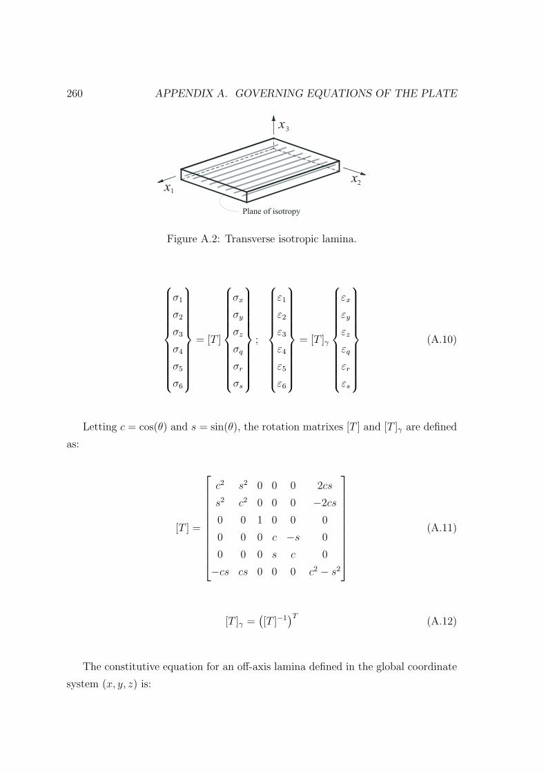
260 APPENDIX A. GOVERNING EQUATIONS OF THE PLATE
Figure A.2: Transverse isotropic lamina.
σ1
σ2
σ3
σ4
σ5
σ6
= [T ]
σx
σy
σz
σq
σr
σs
;
ε1
ε2
ε3
ε4
ε5
ε6
= [T ]γ
εx
εy
εz
εq
εr
εs
(A.10)
Letting c = cos(θ) and s = sin(θ), the rotation matrixes [T ] and [T ]γ are defined
as:
[T ] =
c2 s2 0 0 0 2cs
s2 c2 0 0 0 −2cs
0 0 1 0 0 0
0 0 0 c −s 0
0 0 0 s c 0
−cs cs 0 0 0 c2 − s2
(A.11)
[T ]γ =([T ]−1
)T(A.12)
The constitutive equation for an off-axis lamina defined in the global coordinate
system (x, y, z) is:

A.1. INGREDIENTS FOR THE DEVELOPMENT OF THE EQUATIONS 261
σx
σy
σz
σq
σr
σs
= [T ]−1[C][T ]γ︸ ︷︷ ︸[C]
εx
εy
εz
εq
εr
εs
(A.13)
where [C] is the second-order stiffness tensor written in matrix form referenced to
the local coordinate system (x1, x2, x3), and [C] is the stiffness tensor referenced to
the global coordinate system (x, y, z).
Figure A.3: Lamina coordinate systems.
A.1.3 Laminate resultants
Assuming unitary width in x and y axes, the resulting in-plane forces Nx, Ny, Nxy
and through-the-thickness shear forces Qx, Qy, and in-plane moments Mx,My,Mxy
of lamina p (see Figure A.4) can be calculated from equilibrium conditions as:
Nx
Ny
Nxy
p
=
∫ zp
zp−1
σx
σy
σxy
p
dz (A.14)
Qx
Qy
p
=
∫ zp
zp−1
σxz
σyz
p
dz (A.15)

262 APPENDIX A. GOVERNING EQUATIONS OF THE PLATE
Mx
My
Mxy
p
=
∫ zp
zp−1
σx
σy
σxy
p
z dz (A.16)
Figure A.4: Force and moment resultants on a lamina (or laminate).
where zp−1 and zp are the thickness coordinates of the bottom and top of lamina
p (see Figure A.5). The superposition of different laminae, with different fiber
orientations or not, configures the laminate. For a laminate with N laminae, the
resulting forces and moments are:
Nx
Ny
Nxy
=
∫ h/2
−h/2
σx
σy
σxy
dz =
N∑
p=1
∫ zp
zp−1
σx
σy
σxy
p
dz (A.17)
Qx
Qy
=
∫ h/2
−h/2
σxz
σyz
dz =
N∑
p=1
∫ zp
zp−1
σxz
σyz
p
dz (A.18)
Mx
My
Mxy
=
∫ h/2
−h/2
σx
σy
σxy
z dz =
N∑
p=1
∫ zp
zp−1
σx
σy
σxy
p
z dz (A.19)
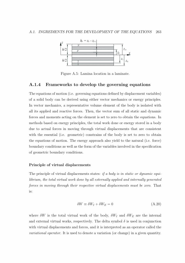
A.1. INGREDIENTS FOR THE DEVELOPMENT OF THE EQUATIONS 263
Figure A.5: Lamina location in a laminate.
A.1.4 Frameworks to develop the governing equations
The equations of motion (i.e. governing equations defined by displacement variables)
of a solid body can be derived using either vector mechanics or energy principles.
In vector mechanics, a representative volume element of the body is isolated with
all its applied and reactive forces. Then, the vector sum of all static and dynamic
forces and moments acting on the element is set to zero to obtain the equations. In
methods based on energy principles, the total work done or energy stored in a body
due to actual forces in moving through virtual displacements that are consistent
with the essential (i.e. geometric) constrains of the body is set to zero to obtain
the equations of motion. The energy approach also yield to the natural (i.e. force)
boundary conditions as well as the form of the variables involved in the specification
of geometric boundary conditions.
Principle of virtual displacements
The principle of virtual displacements states: if a body is in static or dynamic equi-
librium, the total virtual work done by all externally applied and internally generated
forces in moving through their respective virtual displacements must be zero. That
is:
δW ≡ δWI + δWE = 0 (A.20)
where δW is the total virtual work of the body, δWI and δWE are the internal
and external virtual works, respectively. The delta symbol δ is used in conjunction
with virtual displacements and forces, and it is interpreted as an operator called the
variational operator. It is used to denote a variation (or change) in a given quantity.

264 APPENDIX A. GOVERNING EQUATIONS OF THE PLATE
The external work done due to virtual displacements δu in a solid body Ω sub-
jected to body forces f per unit of mass and surface tractions T per unit area of the
boundary Γσ is given by:
δWE = −∫
Ω
ρf · δu dv −∫
Γσ
T · δu ds (A.21)
where ρ is the density, ds denotes a surface element, dv denotes a volume element
and Γσ denotes the portion of the boundary in which the stresses are specified. The
negative sign of Equation (A.21) indicates that the work is performed on the body.
The external virtual work can also be done due to virtual body forces and surface
tractions, which yield to called complementary virtual work.
The forces applied on a deformable body cause it to deform and the body ex-
periences internal stresses. The relative movement of the material particles in the
body can be measured in terms of strains. Therefore, the work done on the body
by external forces is responsible for the internal work. The internal virtual work is
also called virtual strain energy and is expressed by:
δWI = δU =
∫
Ω
σ : δε dv (A.22)
where σ is the stress tensor and δε is the virtual strain tensor due to the virtual
displacement δu.
Replacing Equations (A.21) and (A.22), the principle of virtual work written in
terms of Cartesian rectangular components yields to (sum on repeated subscripts is
implied):
∫
Ω
(σijδεij − ρfiδui) dv −∫
Γσ
Tiδui ds = 0; i, j = 1, 2, 3 (A.23)
By means of the fundamental lemma of variational calculus [61], the principle of
virtual works can be expressed by differential equations called Euler-Lagrange equa-
tions. These equations are the usually form used to write the governing equations.
Hamilton principle
The Hamilton principle states that of all possible paths that a material particle could
travel from its position at time t1 to its position at time t2, its actual path will be

A.1. INGREDIENTS FOR THE DEVELOPMENT OF THE EQUATIONS 265
one for which the following integral is an extremum:
∫ t2
t1
(K −W ) dt (A.24)
The difference between the kinetic and potential energies is called the Lagrangian
function:
L = K −W = K −WI −WE (A.25)
Thus, Hamilton principle can be expressed as:
∫ t2
t1
(δK − δWI − δWE) dt = 0 (A.26)
The kinetic energy of a continuous body Ω is given by:
K =1
2
∫
Ω
ρ∂u
∂t· ∂u
∂tdv (A.27)
where∂u
∂tdenotes the velocity of the material particle.
Principle of minimum total potential energy
A special case of the principle of virtual displacements is the principle of minimum
total potential energy. The difference between the principle of virtual displacements
and the principle of minimum total potential energy is that, in the latter a consti-
tutive law is invoked. Thus, the principle of virtual displacements is more general
and it is applied to all material bodies independent of their constitutive behavior.
The sum U + V = Π is called the total potential energy of the elastic body,
where V is a potential equal to WE and U is the strain energy which is equal to
WI . The principle of minimum total potential energy states that: of all admissible
displacements, those that satisfy the equilibrium equations make the total potential
energy a minimum. Thus, the principle of virtual work takes the form:
∂U + ∂V ≡ ∂Π = 0 (A.28)
The Euler-Lagrange equations resulting from the principle of virtual displace-
ments are always in terms of the stresses or stress resultants, whereas those from

266 APPENDIX A. GOVERNING EQUATIONS OF THE PLATE
the principle of minimum total potential energy are in terms of the strains or dis-
placements.
Variational methods
In general, exact solutions for the dynamic response of rectangular and flat plates
with a certain boundary conditions are not available. Under these circumstances,
methods known as classical variational methods can be applied (e.g. Ritz method ;
Galerkin method).
In variational methods it is seek an approximate solution to the problem in
terms of adjustable parameters that are determined by substituting the assumed
solution into the energy principle (∂W = 0 or ∂Π = 0) that is equivalent to the
governing equations of the problem. Such solution methods are called direct methods
because the approximate solutions are obtained directly by applying the same energy
principle that was used to derive the governing equations. The assumed solutions in
the energy methods are in the form of a finite linear combination of undetermined
parameters and appropriately chosen functions. Since the solution of a continuum
problem, in general, cannot be represented by a infinite set of functions, error is
introduced into the solution.
In the Ritz method, a dependent unknown displacement u is approximated by a
finite linear combination UN of the form:
u ≈ UN =N∑
j=1
cjϕj + ϕ0 (A.29)
where ϕ0 represents the particular solution, while∑cjϕj is the homogeneous part
of the solution. cj denote undetermined parameters and ϕj are called the approx-
imation functions which are appropriately selected functions of position. In order
to ensure that the algebraic equations resulting from the Ritz approximation have
a solution which converges to the true solution of the problem as the number of
parameters N is increased, the approximation functions have to satisfy some re-
quirements:
1. ϕj(j = 1, 2, . . . , N) should satisfy the following three conditions:

A.1. INGREDIENTS FOR THE DEVELOPMENT OF THE EQUATIONS 267
(a) Each ϕj is continuous, as required in the variational statement (i.e. ∂W =
0 or ∂Π = 0).
(b) Each ϕj satisfies the homogeneous form of the specified essential bound-
ary conditions.
(c) The set ϕj is linearly independent and complete.
2. ϕ0 has to satisfy only the specified essential boundary conditions associated
with the variational formulation since the natural boundary conditions are
included in the functional Π or the statement δW ; ϕ0 plays the role of the
particular solution. It is necessarily equal to zero when the specified essential
boundary conditions are homogeneous.
Once the approximation functions ϕ0 and ϕj are selected, the parameters cj in
Equation (A.29) are determined by requiring UN to minimize the total potential
energy functional Π or satisfy the principle of virtual displacements of the problem.
For the principle of minimum total potential energy, upon substitution of the
approximation u ≈ UN , Π(UN) becomes a function of c1, c1, . . . , cN . Hence, min-
imization of the functional Π(c1, c1, . . . , cN) is reduced to the minimization of a
function of several variables:
0 = δΠ(UN) =N∑
j=1
δΠ
δcjcj or
δΠ
δcj= 0 (A.30)
The same procedure applies to the principle of virtual displacements. That is:
0 = δW (UN) =N∑
j=1
δW
δcjcj or
δW
δcj= 0 (A.31)
Equation (A.30) or (A.31) gives N algebraic equations in the N coefficients
(c1, c2, . . . , cN),
0 =δΠ
δcj=
N∑
j=1
Rijcj − Fi or Rc = F (A.32)
where Rij and Fi are known coefficients that depend on the problem parameters
(e.g. geometry, material coefficients and loads) and the approximation functions.

268 APPENDIX A. GOVERNING EQUATIONS OF THE PLATE
Equation (A.32) is then solved for ci and substituted back into Equation (A.29) to
obtain the Ritz solution with N parameters.
A.2 Plate theories and governing equations
A plate is a structural element with planform dimensions that are large compared to
its thickness and is subjected to loads that cause bending deformation in addition to
stretching. Because of the smallness of thickness dimension, it is often not necessary
to model them using 3D elasticity equations. Simple 2D plate theories can be
developed by making assumptions concerning the variation of the displacement field.
Therefore, the compatibility conditions which provide single-valued solution of the
displacements by means of the strain-displacement relations (i.e. Equations (A.1))
are not necessary since the displacements are directly assumed.
In this section only are shown the resulting governing equations for the classical
laminated plate theory and for the first-order shear plate theory. These plate theories
are the most easier and used in the literature in order to develop complete analytical
impact models of laminated composite plates. Other more accurate plate theories
can be used but are often dismissed since the development of the governing equations
becomes algebraic complicated and their integration imply high computational effort
without improving significantly the accuracy of the results.
A.2.1 Classical laminated plate theory
Displacement field and kinematics
The displacement field of the classical laminated plate theory is based on the Kirchhoff-
Love hypothesis, which involve the following assumptions:
1. Straight lines perpendicular to the mid-plane (i.e. transverse normals) before
deformations remain straight after deformation.
2. The transverse normals do not experience elongation (i.e. they are inextensi-
ble).
3. The transverse normals rotate such that they remain perpendicular to the
mid-plane after deformation.

A.2. PLATE THEORIES AND GOVERNING EQUATIONS 269
The first two assumptions of the hypothesis require that in-plane displacements
u and v vary linearly through-the-thickness of the laminate, and the transverse
displacement w is constant through-the-thickness of the laminate (see Figure A.6).
That is:
u(x, y, z) = uo(x, y) + zφ1(x, y)
v(x, y, z) = vo(x, y) + zφ2(x, y)
w(x, y, z) = wo(x, y)
(A.33)
where uo, vo, wo are the displacement components of a point on the mid-plane of
the laminate, φ1 is the rotation of a transverse normal about the y axis, and φ2 is
the rotation of a transverse normal about the x axis. The third assumption of the
Kirchhoff-Love hypothesis implies that the rotations φ1 and φ2 are equal to:
φ1 = −∂wo∂x
; φ2 = −∂wo∂y
(A.34)
Figure A.6: Behavior of transverse section in classical plate theory.
Using the von Karman strain-displacement relations (Equations (A.4)) refer-
enced to the coordinate system (x, y, z) and the assumed displacement field (Equa-
tions (A.33) and (A.34)) the strain components yield to the following expressions:

270 APPENDIX A. GOVERNING EQUATIONS OF THE PLATE
εx ≡ εxx =∂u
∂x+
1
2
(∂w
∂x
)2
=∂uo∂x
+1
2
(∂wo∂x
)2
− z∂2wo∂x2
εy ≡ εyy =∂v
∂y+
1
2
(∂w
∂y
)2
=∂vo∂y
+1
2
(∂wo∂y
)2
− z∂2wo∂y2
εz ≡ εzz =∂w
∂z=∂wo∂z
= 0
εq ≡ 2εyz =∂v
∂z+∂w
∂y= −∂wo
∂y+∂wo∂y
= 0
εr ≡ 2εxz =∂u
∂z+∂w
∂x= −∂wo
∂x+∂wo∂x
= 0
εs ≡ 2εxy =∂u
∂y+∂v
∂x+∂w
∂x
∂w
∂y=∂uo∂y
+∂vo∂x
+∂wo∂x
∂wo∂y− 2z
∂2wo∂x∂y
(A.35)
The three assumptions considered lead to the neglect of the transverse strains εxz,
εyz and εz. Neglecting these strains leads to the omission of σxz, σyz and σz. Thus
the classical laminated plate theory does not account for out-of-plane deformations
and stresses. This implies that plates are infinitely rigid in the transverse direction,
whereas in reality laminated composite plates are weaker in this direction.
Equations (A.35) can be expressed in a general form by:
εi = εoi + zκi; i = x, y, s (A.36)
The strains εoi =(εox, ε
oy, ε
os
)are associated with the in-plane stretching and
shearing of the mid-plane, and are called the membrane strains. The quantities
κi = (κx, κy, κs) are the curvatures which multiplied by z gives the bending strains.
Equations (A.35) shows that membrane strains and curvatures for the classic lami-
nate plate theory have the following explicit form:
εox =∂uo∂x
+1
2
(∂wo∂x
)2
, κx = −∂2wo∂x2
εoy =∂vo∂y
+1
2
(∂wo∂y
)2
, κy = −∂2wo∂y2
εos =∂uo∂y
+∂vo∂x
+∂wo∂x
∂wo∂y
, κs = −2∂2wo∂x∂y
(A.37)
where the underlined terms are the von Karman nonlinear strains.

A.2. PLATE THEORIES AND GOVERNING EQUATIONS 271
Laminate resultants
The in-plane laminate forces (A.17) and moment resultants (A.19) can be expressed
in function of the membrane strains and curvatures resulted in the classical lami-
nated plate theory (Equation (A.36)) by replacing the constitutive equation of each
lamina (Equation (A.13)) of the laminate (see Figure A.5), referenced to the coor-
dinate system (x, y, z). The in-plane resultants of the laminated plate yield to:
Nx
Ny
Nxy
=
A11 A12 A16
A12 A22 A26
A16 A26 A66
εox
εoy
εos
+
B11 B12 B16
B12 B22 B26
B16 B26 B66
κx
κy
κs
(A.38)
Mx
My
Mxy
=
B11 B12 B16
B12 B22 B26
B16 B26 B66
εox
εoy
εos
+
D11 D12 D16
D12 D22 D26
D16 D26 D66
κx
κy
κs
(A.39)
where Aij denote the extensional stiffness, Bij the bending-extensional coupling
stiffness, and Dij the bending stiffness of a laminate. They are defined by:
Aij =N∑
p=1
Cij,p (zp − zp−1) ; i, j = 1, 2, 6 (A.40)
Bij =1
2
N∑
p=1
Cij,p
(z2p − z2
p−1
); i, j = 1, 2, 6 (A.41)
Dij =1
3
N∑
p=1
Cij,p
(z3p − z3
p−1
); i, j = 1, 2, 6 (A.42)
Governing equations
The boundary conditions considered for the test ASTM - D7136 / D7136M [59] are
approximated to simply supported boundary conditions. In this case, the appli-
cation of a variational method is not necessary since the assumed solutions of the
displacements provided by the Navier solutions yield, for some laminate configu-
rations, to the exact solution of the governing equations. Therefore, the governing
equations are obtained by applying the Hamilton principle.

272 APPENDIX A. GOVERNING EQUATIONS OF THE PLATE
The virtual strain energy for classical plate theory in a solid element of the plate
is done by:
δU =
∫
Ω
(σxδεx + σyδεy + σsδεs) dv (A.43)
By replacing the assumed kinematics (Equation (A.36)) and the stress resultants
of the laminate (Equations (A.17) and (A.19)), the virtual strain energy results:
δU =
∫
Ω
(Nxδε
ox +Mxδκx +Nyδε
oy +Myδκy +Nxyδε
os +Mxyδκs
)dxdy (A.44)
The virtual kinetic energy is defined by:
δK =
∫
Ω
∫ h/2
−h/2ρ (uδu+ vδv + wδw) dz dxdy (A.45)
where the superposed dot indicates first derivative respect time. By replacing the
assumed displacement field (Equations (A.33)) and integrating over the plate thick-
ness, the virtual kinetic energy yields to:
δK =
∫
Ω
[−I1 (uoδuo + voδvo + woδwo) + I2
(∂δwo∂x
uo
+∂wo∂x
δuo +∂δwo∂y
vo +∂wo∂y
δvo
)− I3
(∂wo∂x
∂δwo∂x
+∂wo∂y
∂δwo∂y
)]dxdy
(A.46)
For laminates composed by plies with the same material and by considering that
the center of masses is located in the laminate centerline, the inertia terms (I1, I2, I3)
are defined by:
I1
I2
I3
=
∫ h/2
−h/2
1
z
z2
ρ dz = ρ
h
0
h3
12
(A.47)
The external applied forces consist of a distributed transverse load q over the
surface located at (x, y,h
2), and forces and moments due to in-plane normal stress

A.2. PLATE THEORIES AND GOVERNING EQUATIONS 273
Figure A.7: Stress resultants on an arbitrary edge of a laminate.
σnn, in-plane tangential stress σns, and transverse shear stress σnz, all acting on and
edge with normal n (see Figure A.7).
Then, the virtual work done by the external forces is:
δV = −∫
Ω
q(x, y)δwo(x, y,h
2) dxdy
−∫
Γσ
∫ h/2
−h/2[σnnδun + σnsδus + σnzδw] dzds
(A.48)
The stresses σnn, σns, and stress σnz can be expressed in force and moment
resultants by:
Nnn
Nns
=
∫ h/2
−h/2
σnn
σns
dz,
Mnn
Mns
=
∫ h/2
−h/2
σnn
σns
z dz
Qn =
∫ h/2
−h/2σnz dz
(A.49)
Applying Hamilton principle, the following Equation (A.50) defined in terms of
the force and moment resultants is obtained:

274 APPENDIX A. GOVERNING EQUATIONS OF THE PLATE
0 =
∫ T
0
∫
Ω
[−(∂Nx
∂x+∂Nxy
∂y− I1uo
)δuo
−(∂Nxy
∂x+∂Ny
∂y− I1vo
)δvo
−(∂2Mx
∂x2+ 2
∂2Mxy
∂x∂y+∂2My
∂y2+N (uo, vo, wo)
+q − I1wo + I3∂2wo∂x2
+ I3∂2wo∂y2
)δwo
]dxdy dt
+
∫ T
0
∫
Γσ
[(Nnn − Nnn
)δuon +
(Nns − Nns
)δuos
+(Vn − Vn
)δwo −
(Mnn − Mnn
) ∂δwo∂n
]ds dt
(A.50)
where N (uo, vo, wo), Vn and Vn are defined by:
N (uo, vo, wo) =∂
∂x
(Nx
∂wo∂x
+Nxy∂wo∂y
)+
∂
∂y
(Nxy
∂wo∂x
+Ny∂wo∂y
)(A.51)
Vn ≡∂Mx
∂xnx +
∂Mxy
∂ynx +
∂My
∂yny +
∂Mxy
∂xny +
∂Mns
∂snx
+P(uo, vo, wo) + I3∂wo∂x
nx + I3∂wo∂y
ny
(A.52)
Vn = Qn +∂Mns
∂s(A.53)
where P(uo, vo, wo) is defined by:
P(uo, vo, wo) =
(Nx
∂wo∂x
+Nxy∂wo∂y
)nx +
(Nxy
∂wo∂x
+Ny∂wo∂y
)ny (A.54)
From Equation (A.50) the Euler-Lagrange governing equations are obtained:
∂Nx
∂x+∂Nxy
∂y= I1uo − I2
∂wo∂x
(A.55)
∂Nxy
∂x+∂Ny
∂y= I1vo − I2
∂wo∂y
(A.56)

A.2. PLATE THEORIES AND GOVERNING EQUATIONS 275
∂2Mx
∂x2+ 2
∂2Mxy
∂x∂y+∂2My
∂y2+N (uo, vo, wo) + q
= I1wo + I2
(∂uo∂x
+∂vo∂y
)− I3
(∂2wo∂x2
+∂2wo∂y2
) (A.57)
where the terms involving I3 are called rotary (or rotatory) inertia terms, and are
often omitted because it is small in comparison to the I1u and I1v.
And the natural boundary conditions [61] are:
Nnn − Nnn = 0, Nns − Nns = 0
Mnn − Mnn = 0, Vn − Vn = 0(A.58)
When transient response of a plate is of interest, it is necessary to know the
initial displacement field and velocity field throughout the domain of the plate. In
classical laminated plate theory, the initial conditions at time t = 0 for all points in
Ω are:
un = u0n, us = u0
s, wo = w0o
un = u0n, us = u0
s, wo = w0o
(A.59)
The governing Equations (A.55-A.57) can be expressed in terms of displacements
uo, vo, wo by substituting Equations (A.38) and (A.39), and the resulting expressions
of the strains (Equations (A.37)). Neglecting the third order derivative terms in the
space, the resulting motion equations are:
∂
∂x
[A11
∂uo∂x
+ A12∂vo∂y
+ A16
(∂uo∂y
+∂vo∂x
)+B11
(−∂
2wo∂x2
)+
B12
(−∂
2wo∂y2
)+B16
(−2
∂2wo∂x∂y
)]+
∂
∂y
[A16
∂uo∂x
+ A26∂vo∂y
+
A66
(∂uo∂y
+∂vo∂x
)+B16
(−∂
2wo∂x2
)+B26
(−∂
2wo∂y2
)
+B66
(−2
∂2wo∂x∂y
)]= I1
∂2uo∂t2− I2
∂wo∂x
(A.60)

276 APPENDIX A. GOVERNING EQUATIONS OF THE PLATE
∂
∂x
[A16
∂uo∂x
+ A26∂vo∂y
+ A66
(∂uo∂y
+∂vo∂x
)+B16
(−∂
2wo∂x2
)
+B26
(−∂
2wo∂y2
)+B66
(−2
∂2wo∂x∂y
)]+
∂
∂y
[A12
∂uo∂x
+ A22∂vo∂y
+A26
(∂uo∂y
+∂vo∂x
)+B12
(−∂
2wo∂x2
)+B22
(−∂
2wo∂y2
)
+B26
(−2
∂2wo∂x∂y
)]= I1
∂2vo∂t2− I2
∂wo∂y
(A.61)
∂2
∂x2
[B11
∂uo∂x
+B12∂vo∂y
+B16
(∂uo∂y
+∂vo∂x
)+D11
(−∂
2wo∂x2
)
+D12
(−∂
2wo∂y2
)+D16
(−2
∂2wo∂x∂y
)]+ 2
∂2
∂x∂y
[B16
∂uo∂x
+B26∂vo∂y
+B66
(∂uo∂y
+∂vo∂x
)+D16
(−∂
2wo∂x2
)
+D26
(−∂
2wo∂y2
)+D66
(−2
∂2wo∂x∂y
)]+
∂2
∂y2
[B12
∂uo∂x
+B22∂vo∂y
+B26
(∂uo∂y
+∂vo∂x
)+D12
(−∂
2wo∂x2
)+D22
(−∂
2wo∂y2
)
+D26
(−2
∂2wo∂x∂y
)]+N (uo, vo, wo) + q = I1
∂2wo∂t2
+I2
(∂uo∂x
+∂vo∂y
)− I3
(∂2wo∂x2
+∂2wo∂y2
)
(A.62)
A.2.2 First-order shear plate theory
The classical laminated plate theory is not recommended for composites that are
likely to fail in transverse shear or delamination, because the transverse shears and
normal stresses are not accounted for. A refinement to the classical plate theory is
provided by the first-order shear deformation plate theory (also known as Mindlin
plate theory). There are numerous plate theories documented in the literature (not
shown here) that also include transverse shear deformations. In all these theories,
the displacements are expanded as linear combinations of the thickness coordinate
and undetermined functions of position in the reference surface.
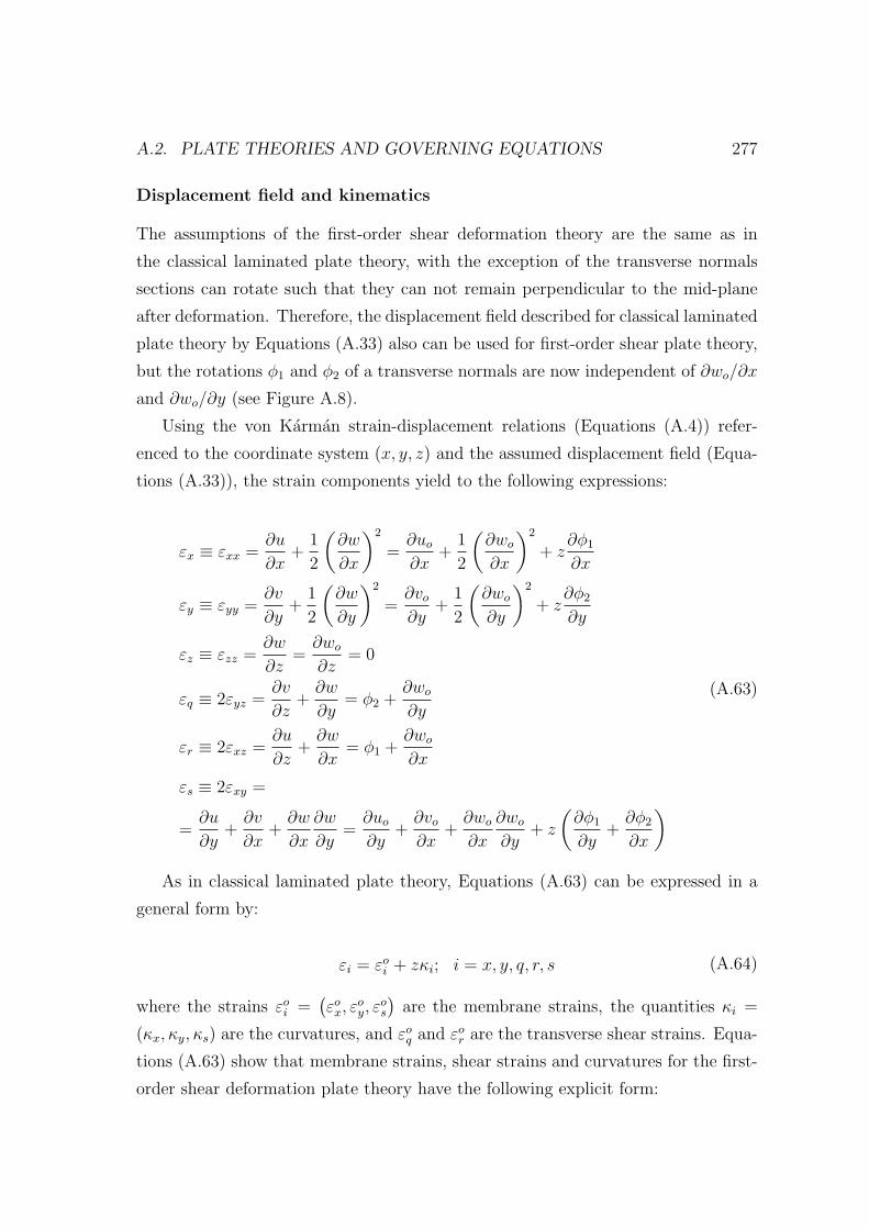
A.2. PLATE THEORIES AND GOVERNING EQUATIONS 277
Displacement field and kinematics
The assumptions of the first-order shear deformation theory are the same as in
the classical laminated plate theory, with the exception of the transverse normals
sections can rotate such that they can not remain perpendicular to the mid-plane
after deformation. Therefore, the displacement field described for classical laminated
plate theory by Equations (A.33) also can be used for first-order shear plate theory,
but the rotations φ1 and φ2 of a transverse normals are now independent of ∂wo/∂x
and ∂wo/∂y (see Figure A.8).
Using the von Karman strain-displacement relations (Equations (A.4)) refer-
enced to the coordinate system (x, y, z) and the assumed displacement field (Equa-
tions (A.33)), the strain components yield to the following expressions:
εx ≡ εxx =∂u
∂x+
1
2
(∂w
∂x
)2
=∂uo∂x
+1
2
(∂wo∂x
)2
+ z∂φ1
∂x
εy ≡ εyy =∂v
∂y+
1
2
(∂w
∂y
)2
=∂vo∂y
+1
2
(∂wo∂y
)2
+ z∂φ2
∂y
εz ≡ εzz =∂w
∂z=∂wo∂z
= 0
εq ≡ 2εyz =∂v
∂z+∂w
∂y= φ2 +
∂wo∂y
εr ≡ 2εxz =∂u
∂z+∂w
∂x= φ1 +
∂wo∂x
εs ≡ 2εxy =
=∂u
∂y+∂v
∂x+∂w
∂x
∂w
∂y=∂uo∂y
+∂vo∂x
+∂wo∂x
∂wo∂y
+ z
(∂φ1
∂y+∂φ2
∂x
)
(A.63)
As in classical laminated plate theory, Equations (A.63) can be expressed in a
general form by:
εi = εoi + zκi; i = x, y, q, r, s (A.64)
where the strains εoi =(εox, ε
oy, ε
os
)are the membrane strains, the quantities κi =
(κx, κy, κs) are the curvatures, and εoq and εor are the transverse shear strains. Equa-
tions (A.63) show that membrane strains, shear strains and curvatures for the first-
order shear deformation plate theory have the following explicit form:

278 APPENDIX A. GOVERNING EQUATIONS OF THE PLATE
Figure A.8: Behavior of transverse section in first-order shear plate theory.
εox =∂uo∂x
+1
2
(∂wo∂x
)2
, κx =∂φ1
∂x
εoy =∂vo∂y
+1
2
(∂wo∂y
)2
, κy =∂φ2
∂y
εoz = 0, κz = 0
εoq = φ2 +∂wo∂y
, κq = 0
εor = φ1 +∂wo∂x
, κr = 0
εos =∂uo∂y
+∂vo∂x
+∂wo∂x
∂wo∂y
, κs =∂φ1
∂y+∂φ2
∂x
(A.65)
where the underlined terms are the von Karman nonlinear strains.
Laminate resultants
The in-plane laminate forces (A.17) and moment resultants (A.19) expressed in
function of the membrane strains and curvatures resulted in the first-order shear
deformation plate theory (Equation (A.64)) yield to the same expressions obtained
for classical laminated plate theory (Equations (A.38) and (A.39)). However, the
transverse shear resultants have also to be defined. Replacing the strains of Equation
(A.64) in the transverse shear forces (A.18) by using the constitutive equation of
each lamina of the laminate referenced to the coordinate system (x, y, z) (Equation
(A.13)), the shear forces result:

A.2. PLATE THEORIES AND GOVERNING EQUATIONS 279
Qy
Qx
=
[A44 A45
A45 A55
]εoq
εor
(A.66)
The transverse shear stiffness Aij are defined by:
Aij = Kij
N∑
p=1
Cij,p (zp − zp−1) ; i, j = 4, 5 (A.67)
where Kij are the dimensionless shear correction factors. Modeling transverse shear
strains and stresses to be constant through the thickness results in the transverse
shear energy being too large when compared to that coming from a more realis-
tic parabolic distribution. In addition, equilibrium is not satisfied at the surfaces.
Therefore, the shear correction factors are used so that the constant distribution
of transverse shear strains and stresses has the same strain energy as the parabolic
distribution. Normally, Kij are taken as an isotropic material (i.e. 5/6).
Governing equations
The virtual strain energy for first-order shear deformation plate theory in a solid
element of the plate is done by:
δU =
∫
Ω
(σxδεx + σyδεy + σsδεs + σqδεq + σrδεr) dv (A.68)
By replacing the assumed kinematics (Equation (A.64)) and the stress resultants
of the laminate (Equations (A.17), (A.18) and (A.19)), the virtual strain energy
results:
δU =
∫
Ω
(Nxδε
ox +Mxδκx +Nyδε
oy +Myδκy +Nxyδε
os
+Mxyδκs +Qxδεor +Qyδε
oq
)dxdy
(A.69)
The virtual kinetic energy was previously defined by Equation (A.45). By re-
placing in the assumed displacement field which coincides with that of classical
laminated plate theory (Equations (A.33)) and integrating over the plate thickness,
the virtual kinetic energy yields to:
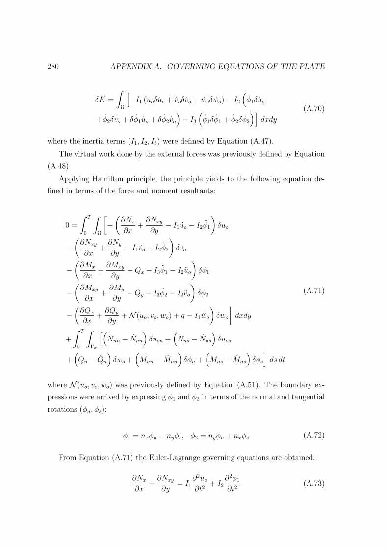
280 APPENDIX A. GOVERNING EQUATIONS OF THE PLATE
δK =
∫
Ω
[−I1 (uoδuo + voδvo + woδwo)− I2
(φ1δuo
+φ2δvo + δφ1uo + δφ2vo
)− I3
(φ1δφ1 + φ2δφ2
)]dxdy
(A.70)
where the inertia terms (I1, I2, I3) were defined by Equation (A.47).
The virtual work done by the external forces was previously defined by Equation
(A.48).
Applying Hamilton principle, the principle yields to the following equation de-
fined in terms of the force and moment resultants:
0 =
∫ T
0
∫
Ω
[−(∂Nx
∂x+∂Nxy
∂y− I1uo − I2φ1
)δuo
−(∂Nxy
∂x+∂Ny
∂y− I1vo − I2φ2
)δvo
−(∂Mx
∂x+∂Mxy
∂y−Qx − I3φ1 − I2uo
)δφ1
−(∂Mxy
∂x+∂My
∂y−Qy − I3φ2 − I2vo
)δφ2
−(∂Qx
∂x+∂Qy
∂y+N (uo, vo, wo) + q − I1wo
)δwo
]dxdy
+
∫ T
0
∫
Γσ
[(Nnn − Nnn
)δuon +
(Nns − Nns
)δuos
+(Qn − Qn
)δwo +
(Mnn − Mnn
)δφn +
(Mns − Mns
)δφs
]ds dt
(A.71)
where N (uo, vo, wo) was previously defined by Equation (A.51). The boundary ex-
pressions were arrived by expressing φ1 and φ2 in terms of the normal and tangential
rotations (φn, φs):
φ1 = nxφn − nyφs, φ2 = nyφn + nxφs (A.72)
From Equation (A.71) the Euler-Lagrange governing equations are obtained:
∂Nx
∂x+∂Nxy
∂y= I1
∂2uo∂t2
+ I2∂2φ1
∂t2(A.73)

A.2. PLATE THEORIES AND GOVERNING EQUATIONS 281
∂Nxy
∂x+∂Ny
∂y= I1
∂2vo∂t2
+ I2∂2φ2
∂t2(A.74)
∂Qx
∂x+∂Qy
∂y+N (uo, vo, wo) + q = I1
∂2wo∂t2
(A.75)
∂Mx
∂x+∂Mxy
∂y−Qx = I3
∂2φ1
∂t2+ I2
∂2uo∂t2
(A.76)
∂Mxy
∂x+∂My
∂y−Qy = I3
∂2φ2
∂t2+ I2
∂2vo∂t2
(A.77)
And the natural boundary conditions [61] are:
Nnn − Nnn = 0, Nns − Nns = 0, Qn − Qn = 0
Mnn − Mnn = 0, Mns − Mns = 0(A.78)
where Qn ≡ Qxnx + Qyny + P(uo, vo, wo). The term P(uo, vo, wo) was previously
defined in Equation (A.54).
The initial conditions of the theory involve specifying the values of the displace-
ments and their first derivatives with respect to time at t = 0 for all points in
Ω:
un = u0n, us = u0
s, wo = w0o, φn = φ0
n, φs = φ0s
un = u0n, us = u0
s, wo = w0o, φn = φ0
n, φs = φ0s
(A.79)
The governing Equations (A.73-A.77) can be expressed in terms of displace-
ments (uo, vo, wo) and rotations (φ1, φ2) by substituting Equations (A.38), (A.39)
and (A.66), and the resulting expressions of the strains (A.65). Neglecting the third
order derivative terms in the space, the resulting motion equations are:
∂
∂x
[A11
∂uo∂x
+ A12∂vo∂y
+ A16
(∂uo∂y
+∂vo∂x
)+B11
∂φ1
∂x
+B12∂φ2
∂y+B16
(∂φ1
∂y+∂φ2
∂x
)]+
∂
∂y
[A16
∂uo∂x
+ A26∂vo∂y
+A66
(∂uo∂y
+∂vo∂x
)+B16
∂φ1
∂x+B26
∂φ2
∂y+B66
(∂φ1
∂y+∂φ2
∂x
)]
= I1∂2uo∂t2
+ I2∂2φ1
∂t2
(A.80)

282 APPENDIX A. GOVERNING EQUATIONS OF THE PLATE
∂
∂x
[A16
∂uo∂x
+ A26∂vo∂y
+ A66
(∂uo∂y
+∂vo∂x
)+B16
∂φ1
∂x
+B26
(∂φ2
∂y
)+B66
(∂φ1
∂y+∂φ2
∂x
)]+
∂
∂y
[A12
∂uo∂x
+ A22∂vo∂y
+A26
(∂uo∂y
+∂vo∂x
)+B12
∂φ1
∂x+B22
∂φ2
∂y+B26
(∂φ1
∂y+∂φ2
∂x
)]
= I1∂2vo∂t2
+ I2∂2φ2
∂t2
(A.81)
∂
∂x
[A45
(∂wo∂y
+ φ2
)+ A55
(∂wo∂x
+ φ1
)]
+∂
∂y
[A44
(∂wo∂y
+ φ2
)+ A45
(∂wo∂x
+ φ1
)]
+N (uo, vo, wo) + q = I1∂2wo∂t2
(A.82)
∂
∂x
[B11
∂uo∂x
+B12∂vo∂y
+B16
(∂uo∂y
+∂vo∂x
)+D11
∂φ1
∂x
+D12
(∂φ2
∂y
)+D16
(∂φ1
∂y+∂φ2
∂x
)]+
∂
∂y
[B16
∂uo∂x
+B26∂vo∂y
+B66
(∂uo∂y
+∂vo∂x
)+D16
∂φ1
∂x+D26
∂φ2
∂y+D66
(∂φ1
∂y+∂φ2
∂x
)]
−[A45
(∂wo∂y
+ φ2
)+ A55
(∂wo∂x
+ φ1
)]= I3
∂2φ1
∂t2+ I2
∂2uo∂t2
(A.83)
∂
∂x
[B16
∂uo∂x
+B26∂vo∂y
+B66
(∂uo∂y
+∂vo∂x
)+D16
∂φ1
∂x
+D26
(∂φ2
∂y
)+D66
(∂φ1
∂y+∂φ2
∂x
)]+
∂
∂y
[B12
∂uo∂x
+B22∂vo∂y
+B26
(∂uo∂y
+∂vo∂x
)+D12
∂φ1
∂x+D22
∂φ2
∂y+D26
(∂φ1
∂y+∂φ2
∂x
)]
−[A44
(∂wo∂y
+ φ2
)+ A45
(∂wo∂x
+ φ1
)]= I3
∂2φ2
∂t2+ I2
∂2vo∂t2
(A.84)