Simulation Metamodelling of Manufacturing Systems with the Use of Artificial Neural Networks

MITIP 2012 Modern Information Technology in the Innovation Processes of Industrial Enterprises

SIMULATION METAMODELLING OF MANUFACTURING SYSTEMS WITH THE USE OF ARTIFICIAL NEURAL NETWORKS

Milan Gregor1, Silvia Palajová2, Michal Gregor3 1,2 Department of Industrial Engineering, University of Zilina,

Univerzitná 1, 010 26 Žilina, Slovakia { milan.gregor ,silvia.palajova}@fstroj.uniza.sk

3Department of Control and Information Systems, University of Zilina, Univerzitná 1, 010 26 Žilina, Slovakia

[email protected]

Abstract:

This paper deals with computer simulation of manufacturing systems and on emulation as an advanced approach of simulation of production and logistic processes. It focuses models going out of simulation models - so called metamodels - as one of the possible ways how to increase effectiveness of simulation optimization and how to reduce the requirements of time-consuming simulation of manufacturing systems. It describes the basis of metamodelling process on specific example of ZIMS and describes neural network metamodels as an universal function approximators.

Keywords:

Simulation, emulation, metamodelling, artificial neural network

1 INTRODUCTION

In today's turbulent environment, a flexibility of manufacturing process is required, which makes a company able to a flexible response on market demands. Except for shortening a production cycle, there are also requests for a high productivity, flexibility of product mix, var-ious production programme, stock reducing, increasing of machine utilization, quality im-provement, rapid responses to emerging problems, delivery time shortening, etc.

It is not possible to handle it, and simultaneously to touch competitive, without continuous improvement of factory processes, implementation of progressive management approaches, technologies, and without rapid decision-making of managers. Decision-making systems provide quality information and provide ahead simulation of possible variants of future sys-tem's behavior, and at the right moment give the opportunity of choice.

Currently, it is axiomatic to solve complex problems by an appropriate computer model that reflects characteristics of a real system or helps to find a solution close to optimal, or directly optimal, for existing or conceptual systems. Therefore, a computer simulation is still gaining major importance. It allows quick testing of various variants of solutions and it minimizes the risk of wrong decisions. This is reflected to considerable economic benefits.

Modern Information Technology in the Innovation Processes of Industrial Enterprises MITIP 2012Modern Information Technology in the Innovation Processes of Industrial Enterprises MITIP 2012Modern Information Technology in the Innovation Processes of Industrial Enterprises MITIP 2012

178178178


Apart from production planning management, production management requires current in-formation about real manufacturing process (feedback from the manufacturing process) in a real time. Those are obtained using the progressive method, which finds application in the management of modern complex systems. It is emulation, which is connection of a real exist-ing system with its parametric simulation model.

Simulation runs are usually computationally difficult and it is not unusual for complex simula-tion models that they last for hours. However, decision making support, exploratory analysis and rapid adaptive calculations often require simplicity for understanding and explanation of representations of reality. Therefore, there are often constructed simpler approximations - models of simulation model - or metamodels which are used for studying of a computer simu-lations' behavior. This is the replacement of empirical data by an appropriate type of theoreti-cal function that adequately describes the original data obtained from the simulation. We call it approximate production management.

For approximation of known data can be also used tools of artificial intelligence. Universal function approximators are artificial neural networks (ANN), which can give adequate output for input signals, regardless of its internal structure. If there is a system whose description is extremely difficult or the system is so complex that its description is almost impossible, but data that enter the system and their corresponding outputs are available, in this situation a suitable ANN can be used. We try to learn it to behave as monitored system by training data (referred inputs and outputs). It is then possible to apply such rules to any input values.

2 SIMULATION OF MANUFACTURING PROCESSES

If there is a simple manufacturing system it can be described by relations and quantitative variables using analytical methods. Analytical methods are too deterministic and static for solving today's complex, dynamic tasks, and mathematical models of complex systems are themselves complex, and there is excluded any possibility of analytical solutions. In such a case model must be studied by simulation.

The first step of computer simulation is to built simulation model of the production system. The next step is to perform experiments with the simulation model and achieved results are used for improvement of the real system. Simulation is a experimental method in which the experiments with a simulation model of manufacturing system are make on a computer. It also ranks among statistical methods because it works on the same theoretical basis as methods of mathematical statistic. Model includes only those characteristics of real system which the analyst is interested. After evaluation of results the analyst makes conclusions about the whole real system, based on experiments with the model.

Simulation overcomes many boundary conditions and limitations of analytical modeling techniques and its use is justified especially in those cases where other possible solutions have failed. It is also an important element in workers' training.

2.1 Parametric simulation model

External information system is often source of data for simulation model. It allows easy transfer and data processing, and it facilitates manipulation with data in database of the model.

Parametric simulation model is a practical tool for finding problems' causes of the selected type of manufacturing systems, created for selected input variables. After modeling and

MITIP 2012 Modern Information Technology in the Innovation Processes of Industrial EnterprisesMITIP 2012 Modern Information Technology in the Innovation Processes of Industrial EnterprisesMITIP 2012 Modern Information Technology in the Innovation Processes of Industrial Enterprises

179179179


entering the specific characteristics of production system (such a service time for each workstation, the way of parts arrival to the workstation, the transportation size, the way of manufacturing system control, etc.) can the process be simulated with sufficient precision. The analyst can also directly see critical points of production process and simulate various possibilities for their removal. The obtained results, in the form of tables or graphs, are after execution of simulation experiments automatically transferred to external information system and on their base optimization of real system can be done. All this can be carried out without detailed knowledge of modeling and simulation methods and without deep knowledge about simulation software. [1]

2.2 Development of simulation of manufacturing systems

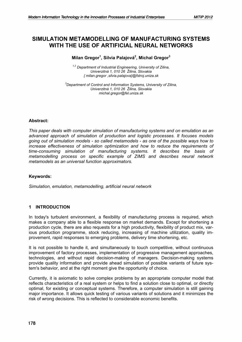
Development of simulation of manufacturing systems at Department of Industrial Engineering (Žilina) is shown in fig. 1. Simulation applications and practical solutions in these areas implemented on our department can be found in other publications, theses, scientific and research projects, and workshops, for example [2], [4], [8], [9], [11], [12], [13].

2.3 Emulation

Feedback from the manufacturing process is provided by systems that collect data from production process. They inform about actual values of process variables from production facilities, and provide an opportunity to intervene in the production process and affect it, to change real system's settings on computer.

Figure 1: Development of simulation


180180180


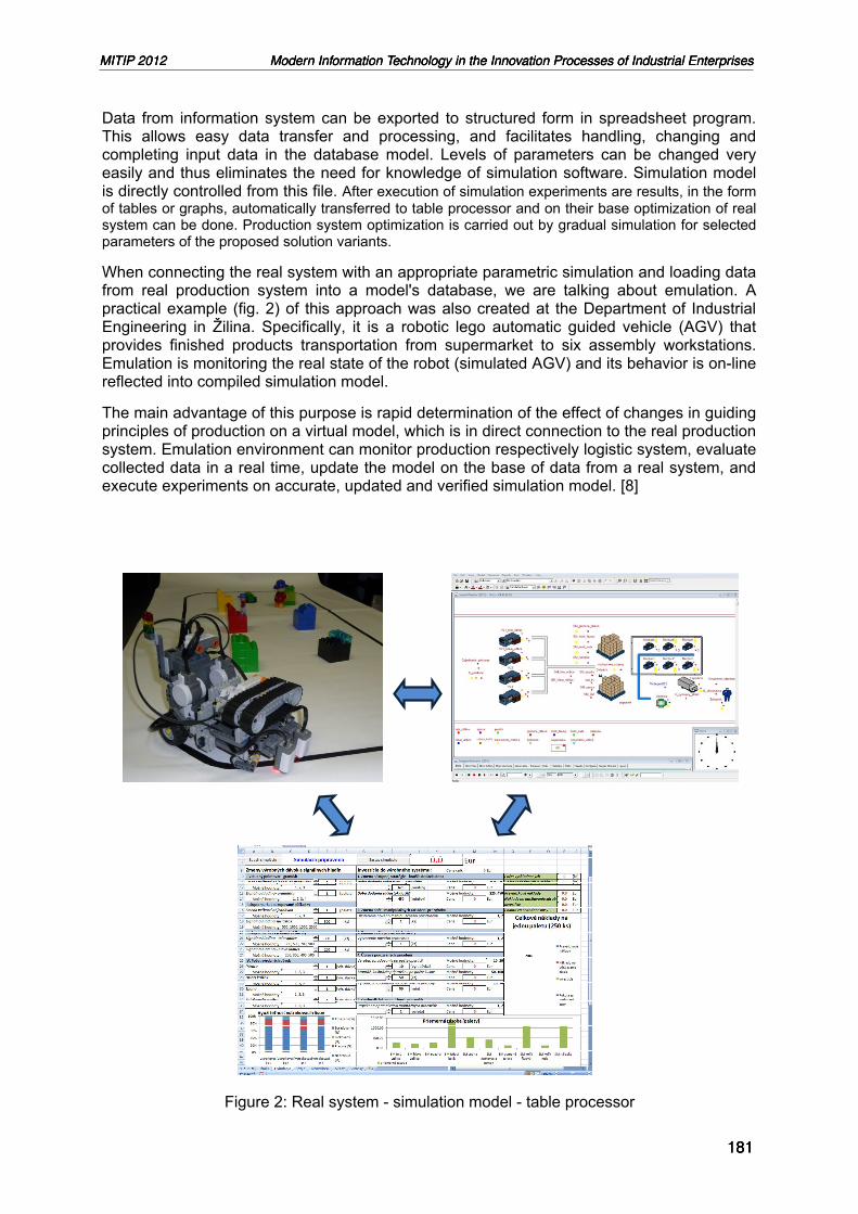
Data from information system can be exported to structured form in spreadsheet program. This allows easy data transfer and processing, and facilitates handling, changing and completing input data in the database model. Levels of parameters can be changed very easily and thus eliminates the need for knowledge of simulation software. Simulation model is directly controlled from this file. After execution of simulation experiments are results, in the form of tables or graphs, automatically transferred to table processor and on their base optimization of real system can be done. Production system optimization is carried out by gradual simulation for selected parameters of the proposed solution variants.

When connecting the real system with an appropriate parametric simulation and loading data from real production system into a model's database, we are talking about emulation. A practical example (fig. 2) of this approach was also created at the Department of Industrial Engineering in Žilina. Specifically, it is a robotic lego automatic guided vehicle (AGV) that provides finished products transportation from supermarket to six assembly workstations. Emulation is monitoring the real state of the robot (simulated AGV) and its behavior is on-line reflected into compiled simulation model.

The main advantage of this purpose is rapid determination of the effect of changes in guiding principles of production on a virtual model, which is in direct connection to the real production system. Emulation environment can monitor production respectively logistic system, evaluate collected data in a real time, update the model on the base of data from a real system, and execute experiments on accurate, updated and verified simulation model. [8]

Figure 2: Real system - simulation model - table processor


181181181


3 SIMULATION METAMODELLING

By collecting data about the system from simulation model we can examine the interdependencies and relationships between variables, and approximate these relations by simplified mathematical expressions. Explanation of basic input-output relationships of the system through a simple mathematical function is the essence of metamodelling. By adoption of metamodels into simulation the computational load of optimization process can be greatly reduced, because computational costs associated with the use of metamodels are much lower than the standard approach of evaluation of all runs with the simulation model.

Metamodels are used to study computer simulations' behavior. They decsribe stochastic (free) dependence, i.e. explained variable is influenced by explanatory variables and also by unpredictable, immeasurable and random effects.

,XfY , (1)

,XfY - regression function, Y – dependent variable, X – vector of values of input factors, ε - vector of random numbers.

3.1 Metamodel creation

Simulation

The creation of metamodel (fig. 3) begins with simulation model in which several simulation runs for different values of input parameters take place. We have created a simulation model of the production cell in concept ZIMS (Zilina Intelligent Manufacturing System - see [3]) that consists of three machines. They gradually tool semiproduct A. The total productivity of the system is affected by the second machine’s failures that occur at specific intervals

60,50,40,30,25,20,15,...,, 1712111 xxxX and repair time is defined by data set 20,15,12,10,8,5x,...,x,xX 2622212 . Our goal is to create a metamodel for average time

which varies due to changes in levels of factors X1 and X2.

Correlation analysis

In order to continue in metamodel making process, it is first necessary to determine whether the observed outputs depend on defined inputs. Therefore, correlation analysis is executed. It detectes variability of dependent variable, which is caused by the considered independent variables. This strength of dependency is expressed by the the correlation coefficient:

yxyx ssxycov

ssyxxyr

, 1,1r

(2)


182182182


r

1jmr12j

r11jj

ini2i1i

y,...,y,yY

x,...,x,xX

Figure 3: Metamodel making process

Condition of mutual independence of the vectors of independent variables Xi must be executed. When this condition is broke, multicollinearity occurs and it means that one variable X is nearly weighted average of the other variables X. It often occurs in small samples. An extreme case is the singularity when one a predictor is exactly linear combination of other predictors. In this case, the regression coefficients can not be standardly calculated. In our data, the condition of input data independence and condition of dependence of outputs on inputs, are executed.

Figure 4: Pearson's correlation coefficients


183183183


Function approximation

In the next step, collected data are replaced with function curve, which describes metamodel and is a reliable approximation of the original output data. Approximated function is estimative function, so some complex function is simpler expressed. Each approximation is accurate at certain interval. According to [6], approximated curve Y(X) should satisfy the following requirements:

characteristic of approximation - Y(X) should pass close to the measured points and be-have in order to fully reflect the information measured in the experiment,

characteristic of relaxation (smoothing) - Y(X) should be "smooth enough" in order to not copy random oscillations in the experimental data that were due to measurement errors and other influences .

These two requirements are in some ways contradictions. Approximated curve due to errors oscillates when it is "too close" to the experimental points. If it is "too smooth", it can be observed away from the original process. Therefore, a good curve is a compromise between two implementation requirements.

There is many kinds of curves and (wave)surfaces. Approximation function may be a linear function (linear combination) of unknown parameters (relation (1)). The most commonly used system of basic functions are polynomial functions and it leads to an approximation of data by polynomials. The linear case is commonly used shape to approximate discrete data. Other forms could be:

logaritmic XY ln10 (3)

exponencial XY 10 (4)

powered 10

XY (5)

hyperbola X

Y 10

(6)

parabola 2210 XXY (7)

To reflect the output data from the simulation we use multiple linear regression model with two regressors and polynomials of various degrees:

i22i110 xxy , (8)

xpxf nn , (9)

Then, based on the found errors, we determine the most appropriate model.

The main task of approximation is to determine the unknown coefficients β in approximation function. The principal types of approximation are interpolation and method of least squares.

Method of least squares

The method determines the estimation of jY of the regression function

pkjjjj bbbxxxfY ,...,,;,...,, 1021 , (10)


184184184


where coefficients pbbb ,...,, 10 are estimations of unknown parameters p ,...,, 10 . The difference between empirical and theoretical value of the dependent variable is the random error [1]:

jjj YYe . (11)

If the random errors apply

22

0

jj

j

eEeD

eE (12)

0, 21 jj eeE for each 21 jj

coefficients pbbb ,...,, 10 may be considered as the best estimates of parameters p ,...,, 10 . (10) shows that random errors have to have a normal distribution with zero mean value (in the case of sufficiently large statistical file) and constant variance (not necessarily, the vari-ance may also vary proportionally). They are independent from Xi and should be mutually independent in pairs. Least-squares condition is that sum of squares of random errors (residual deviations) of de-pendent variable has to be minimal:

min,...,,1

210

n

jjjp YYbbbF . (13)

Coefficients pbbb ,...,, 10 have to be suitable to this requirement. If also a specific type of func-tion (10) is known, it can be inducted into relationship (13) and look for a minimum of the function. The result of the partial derivations of the function pbbbF ,...,, 10 is then set up to be equal to zero:

0

,...,, 10

i

p

bbbbF

i = 0, 1, 2, ..., p. (14)

and the unknown coefficients pbbb ,...,, 10 are calculated by solving of a system of (p + 1)

equations about (p + 1) unknown quantities pbbb ,...,, 10 . A main disadvantage of the method of least squares is its sensitivity to extreme values and the only one outlier can change a direction of the regression line. Therefore the regression analysis should always start with looking over X-Y chart [8].

Computed coefficients for multiple linear regression model with two regressors are:

3765,3161735,64199,18

0

1

2

bbb

(15)

Metamodel validation

The values of the vector β are used for creating of curves that describe the metamodel. In order to check a suitability of the metamodel for intended purposes, validation of the


185185185


metamodel (by comparison of metamodel with simulation output data using mathematical statistics) is done. The graphical representation of metamodel's inputs – outputs relationships provides a simple presentation of expected system behavior, often known as the approximate control.

Errors of approximation functions are in this table:

Error Polynomials of various degrees: Regression

model II III IV V VI MAE 7,6824 1,978 0,5021 0,1722 0,0678 28,5174 MSE 86,6012 5,6888 0,4001 0,0514 0,0081 1166,162 MAPE 2,9705 0,7431 0,1911 0,0637 0,023 0,1108 R^2 0,9952 0,9997 1 1 1 0,9352

As shown, the higher degree polynomial was used, the smaller errors are and higher coefficient of determination. But do not forget that the low degree polynomials do not have enough ability to approximate the data values, and polynomials of higher degrees tend to fluctuations in values between provided data, particularly in border areas. Elements of IV. a higher level do not affect the outcome, because the coefficients from b11 until b28 have values close to zero and polynomials of IV. - VI. degree lose significance. Therefore, in this case it is sufficient to consider the polynomial of maximum III. degree:

32

2212

21

31

22

212121

0144,0015,00024,00029,05309,17922,04314,0335,6035,20408,301

xxxxxxxxxxxxy

(16)

3.2 Metamodel based on Artificial Neural Networks

An approximator of the collected data can also be implemented using an artificial neural network. Artificial neural networks are known for their generalization capabilities, which allow them to be trained to perform regression using supervised learning methods such as backpropagation, Rprop, iRprop, Levenberg-Marquardt, ... [5], [7]. Thus, when provided with a sample of the data, an artificial neural network (ANN) can be constructed and trained to perform regression. Its generalization capability should ensure that results for yet unseen data points are approximately true.

In our case, if we provide a set of input values, simulation provides us with the corresponding desired output values. These input-output pairs have been used to construct a data set. The data set has been divided into two parts – the training data set and the validation data set – as is customary. We have tested several learning algorithms, most notably the aforementioned Rprop algorithm and the Levenberg-Marquardt approach. We have selected Rprop in the end: although the Levenberg-Marquardt approach seems to converge faster, we have found its generalization capability largely unsatisfactory for our purposes. In all following experiments Rprop has been used to implement supervised learning.

One of the widely-known disadvantages of ANNs is the lack of a comprehensive method of selecting the most appropriate architecture for a given task. There is no universal way to determine the optimal number of neurons, layers, or the shape of activation functions. The usual approach therefore is to use trial-and-error to find an appropriate architecture.


186186186


Let us now present the architecture for which we have achieved the best results: the ANN used in this work is a simple feed-forward ANN with completely interconnected adjacent layers. There are two hidden layers, each containing 20 neurons. The activation functions used are: a linear activation function for the first layer; a sigmoid function for the second layer; and a linear activation function for the output layer.

The maximum number of training epochs was set to 4000 and the desired error (the threshold value at which training stops) was set to 1e-10.

Let us now briefly consider the results. Fig. 5 shows the result of training – we can compare the data points corresponding to the desired output with data points corresponding to real outputs of the ANN. The data points are connected by lines so as to facilitate comparison. As we can see from Fig. 5, Fig. 7 and Fig. 8, the approximation error of the ANN is negligible.

In Fig. 6, the difference between the desired and the real output is shown for each sample of the training data set. In Fig. 7, on the other hand, we present the relative error (E = (D – O)/D, where D is the desired output and O the real output).

Figure 5: Training data set – desired out-puts and real outputs

Figure 6: Validation data set – desired outputs and real outputs

As for the validation data set, the desired and real outputs are shown in Fig. 6, while the estimation error and the relative estimation error are shown in Fig. 9 and Fig. 10. As shown, for most data points the relative errors fall within the 1% margin. However, for the second data point, the error is significantly larger, approaching 6%. Upon closer inspection, we have discovered that this particular data point (as well as the last data point presented in Fig. 10) does not fall into the range of values of X1 and X2 used to train the network ( 6050...20151 ,,,,=X , 2012...,5,8,2 ,=X ). This shows that the network can be used to estimate outputs for data points outside of this range, but we should expect greater estimation errors in such cases.


187187187


Figure 7: Approximation errors for samples of the training data set

Figure 8: Relative errors for samples of the training data set

Figure 9: Estimation errors for samples of

the validation data set

Figure 10: Relative errors for samples of the validation data set

4 CONCLUSION

Mathematical models are usually used for systems' experimentation. They represent system in terms of logical and quantitative relationships that can be manipulated and changed in order to find out how the model responds, so as the real system would respond. Many systems are quite difficult for application analytical solutions on them. There can also occur uncertain conditions with insufficient information and without possibility of solution demarcation. In such a case, model must be studied by means of simulation. As well as these models are too complex, their appropriate approximations - called metamodels - are constructed. They relate output simulation data to metamodel's inputs and take into account the random effects occurring in the process. Simulation metamodelling is an appropriate tool for managing and optimization of complex manufacturing systems.


188188188


REFERENCES

[1] FIGA, Š. - PALAJOVÁ, S. (2011): Využitie progresívnych prístupov v simulácii výrobných systémov. MOPP 2011 - Modelování a optimalizace podnikových procesů. Plzeň, 2011. 13. ročník mezinárodního semináře. ISBN 978-80-261-0060-7.

[2] GREGOR, M. - ŠKORÍK, P. (2009): Optimalizácia ako nástroj pre efektívne využívanie simulácie výrobných a logistických systémov. In InvEnt 2009, 2009.

[3] GREGOR, M. - MEDVECKÝ, Š. - MIČIETA, B. (2010): ZIMS- Zilina Intelligent Manufacturing System: study. Žilina : University of Žilina, 2010, p. 35.

[4] Hromada, J. (2004): Simulácia výrobných systémov: doktorandská dizertačná práca. Žilina : ŽU, 2004. 128 p.

[5] IGEL, C. – TOUSSAINT, M. – WEISHUI, W. (2012): Rprop Using the Natural Gradient. Trends and applications in constructive Approximation. Berlin: Birkhäuser Verlag, 2005. Pp. 259-272. ISBN 3-7643-7124-2. URL: http://www.springerlink.com/index/R26X46P536882687.pdf, last accessed 20 May 2012.

[6] KAUKIČ, M. (1998): Numerická analýza I. : Základné problémy a metódy. Žilina : MC Energy s. r. o., 1998. 202 p. ISBN 80-968016-6-X.

[7] KROSE, B. – SMAGT, P.V.D. (1996): An Introduction to Neural Networks. The University of Amsterdam, 1996. URL: http://www.cs.unibo.it/babaoglu/courses/cas/resources/tutorials/Neural_Nets.pdf, last accessed 20 May 2012.

[8] PALAJOVÁ, S. - FIGA, Š. (2011): Pokrokový prístup simulácie výrobných a logistických procesov. Digitálny podnik 2011. Žilina : CEIT SK, s.r.o., 2011. ISBN 978-80-970440-1-5.

[9] PALAJOVÁ, S. - FIGA, Š. - GREGOR, M. (2011): Simulation of manufacturing and logistics systems for the 21th century. Applied computer science : management of production processes. ISSN 1895-3735, 2011, Vol. 7, no. 2.

[10] RIMARČÍK, M. (2007): Štatistika pre prax. Košice : Vydané nákladom vlastným, 2007. 200 p. ISBN 978-80-969813-1-1.

[11] ŠKORÍK, P. - GREGOR, M. - ŠTEFÁNIK, A. (2009): Artificial intelligence tools in simulation and optimization of production systems. Applied computer science, 2009.

[12] ŠKORÍK, P. (2009): Simulácia výrobných systémov s podporou virtuálnej reality: doktorandská dizertačná práca. Žilina : ŽU, 2009. 125 p.

[13] ŠTEFÁNIK, A. - ŠKORÍK, P. (2009): Parametrická tvorba 3D simulačných modelov v praxi. Produktivita a inovácie 6/2009.

ACKNOWLEDGEMENT

This paper is the part of research supported by: VEGA 1/1146/12.


189189189

Simulation Metamodelling of Manufacturing Systems with the Use of Artificial Neural Networks

Documents

Transcript of Simulation Metamodelling of Manufacturing Systems with the Use of Artificial Neural Networks