
Monitoring the Bifurcated Recurrent Laryngeal Nerve - Journal ...
Upload
khangminh22Category
view
6download
0
Departamento de Electronica FısicaEscuela Tecnica Superior de Ingenieros de Telecomunicacion
Artificial recurrent neural networks for
the distributed control of electrical
grids with photovoltaic electricity
Autor:
Eduardo Matallanas de AvilaIngeniero de Telecomunicacion
Directores:
Estefanıa Caamano Martın Alvaro Gutierrez MartınDra. Ingeniera de Telecomunicacion Dr. Ingeniero de Telecomunicacion
2016


Tribunal nombrado por el Mgfco. y Excmo. Sr. Rector de la Universidad Politecnica
de Madrid.
Presidente/a: Dr. D. Felix Monasterio-Huelin Macia
Secretario/a: Dr. D. Miguel A. Egido Aguilera
Vocal 1: Dr. D. Leocadio Hontoria Garcıa
Vocal 2: Dr. D. Inaki Navarro Oiza
Vocal 3: Dr. D. Anders Lyhne Christensen
Suplente 1: Dr. D. Pablo Dıaz Villar
Suplente 2: Dr. D. Manuel Castillo Cagigal
Realizando el acto de defensa y lectura de la Tesis en la E.T.S.I.T., Madrid,
el dıa de de 2016.
Acuerdan otorgar la calificacion de:
Y, para que conste, se extiende firmada por los componentes del tribunal, la presentediligencia
El/La Presidente/a El/La Secretario/a
Fdo: Fdo:
El/La Vocal 1 El/La Vocal 2 El/La Vocal 3
Fdo: Fdo: Fdo:

Resumen
El sistema electrico actual no ha evolucionado desde sus orıgenes. Esto ha hechoque emerjan diferentes problemas los cuales son necesarios afrontar para incrementarel rendimiento de las redes electricas. Uno de estos problemas es el crecimientode la demanda, mientras que otros, como las Tecnologıas de la Informacion y lasComunicaciones (TIC) o la Generacion Distribuida (GD), se han desarrollado dentrode la red electrica recientemente sin ser propiamente integradas dentro de ella. EstaTesis afronta los problemas derivados del manejo y la operacion de las redes electricasexistentes y su evolucion hacia lo que se considera la red electrica del futuro o SmartGrid (SG).
El SG nace de la convergencia de cinco aspectos: i) la red electrica, ii) TICs,iii) energıas renovables, iv) almacenamiento electrico y v) Gestion de la DemandaElectrica (GDE). Esta Tesis consiste en un primer paso hacia el SG uniendo eintegrando los cinco aspectos claves para su desarrollo y despliegue en el futurocercano. Para ello, la mejora del estado de la red electrica se consigue a traves delsuavizado del consumo agregado. Para lograr este objetivo, se propone el uso de unalgoritmo que procese la informacion proveniente de las TICs para que todas laspartes de la red electrica se puedan beneficiar. Algunos de estos beneficios son: mejoruso de las infraestructuras, reduccion de su tamano, mayor eficiencia, reduccion decostes e integracion de GD, entre otros. El algoritmo propuesto esta basado en unaaproximacion distribuida en la que los usuarios son hechos partıcipes de sus decisiones,siendo capaces de manejar sus flujos de potencia con este objetivo. El algoritmose ha implementado siguiendo una estrategia basada en la GDE combinada con elcontrol automatico de la demanda que ayude a integrar los Recursos EnergeticosDistribuidos (RED) (energıas renovables y sistemas de almacenamiento electrico),que lo conducen hacia un concepto innovador denominado Gestion de la Activa de laDemanda Electrica (GADE).
En esta Tesis, una aproximacion basada en la Inteligencia Artificial (IA) hasido utilizada para implementar el algoritmo propuesto. Este algoritmo ha sidoconstruido utilizando Redes Neuronales Artificiales (RNAs), mas concretamenteRedes Neuronales Recurrentes (RNRs). El uso de RNAs ha sido motivado porlas ventajas de trabajar con sistemas distribuidos, adaptativos y no lineales. Y laeleccion de las RNRs se ha basado en sus propiedades dinamicas, las cuales encajanperfectamente con el comportamiento dinamico no lineal de la red electrica. Ademas,un controlador neural es utilizado para manejar cada elemento de la red electrica,incrementado la eficiencia global a traves del suavizado del consumo agregado ymaximizando el autoconsumo de los RED disponibles. Sin embargo, no existe ninguntipo de comunicacion entre los distintos individuos y la unica informacion disponiblees el consumo agregado de la red electrica. Finalmente, la mejora de la red electrica seha conseguido de manera colectiva utilizando el algoritmo propuesto para coordinarla respuesta del conjunto de controladores neuronales.


Abstract
The present electrical systems have not evolved since its inception. This fact hastriggered the emergence of different problems which are necessary to tackle in orderto enhance the grid performance. The demand growth is one of these problems, whileothers, such as the Information and Communications Technology (ICT) or DistributedGeneration (DG), have been recently developed inside the grid without their properintegration. This Thesis addresses the problems arising from the management andoperation of existing electrical grids and their evolution to what is considered the gridof the future or Smart Grid (SG).
The SG is born from the convergence of five aspects: i) the grid, ii) ICTs,iii) renewable energies, iv) Electrical Energy Storages (EESs) and v) Demand SideManagement (DSM). This Thesis consists of a first step towards the SG by linkingand integrating the five key aspects for its development and deployment in the nearfuture. To this end, the enhancement of the grid status is achieved by the smoothnessof the aggregated consumption. In order to fulfill this objective, an algorithm has beenproposed that processes the data gathered from the ICTs to benefit all the parts ofthe grid. Some of these benefits are: better use of the infrastructure, reduction in itssize, greater operational efficiency, cost reductions and integration of the DG, amongothers. The proposed algorithm is based on a decentralized approximation in whichthe users are made participants in their decisions, being able to manage their powerflows into this objective. It is implemented following DSM techniques combined withan automatic control of demand that helps to integrate Distributed Energy Resources(DER) (renewable energies and EESs), which leads to an innovative concept calledActive Demand Side Management (ADSM).
In this Thesis, an Artificial Intelligence (AI) approach was used to implement theproposed algorithm. This algorithm is built based on Artificial Neural Networks(ANNs), specifically Recurrent Neural Networks (RNNs). The use of ANNs ismotivated by the advantages of working with distributed, adaptive and nonlinearsystems. And the election of RNNs is based on their dynamic behavior, which fitsperfectly with the nonlinear dynamic behavior of the grid. In addition, a neuralcontroller is used to operate in each element of the grid to increase the global efficiencyby smoothing the aggregated consumption and to maximize the local self-consumptionof the available DER. However, there is no communication among the users and theavailable information is only the aggregated consumption of the grid. Finally, theenhancement of the grid is achieved collectively by using the proposed algorithm tocoordinate the responses of the neural controller ensemble.


To my Family


Acknowledgements
After all these years, it is extremely difficult to condense all the thanks to allthose involved in the development of the Thesis. But I have already finished myPh.D. without dying in the process, so I think I will be able to do it.
First of all, I am truly grateful to my supervisors Prof. Alvaro Gutierrez Martınand Prof. Estefanıa Caamano Martın for the opportunity they gave me to takethis path. Alvaro is like my science father while Estefanıa is my science mother.Alvaro is the culprit that started this madness and I really thank his effort andconstant support to the development of this Thesis. He always had time to discussand search for a solution to all the problems found during the development of theThesis. He has also put up with me during these years. For all his support and help,my deepest gratitude Alvaro. On the other hand, I would like to thank Estefanıa allher concerns and interests in the work done during the development of this Thesis.She was very supportive and thorough review of the work done has been a source ofvaluable improvements.
I am grateful to have been part of the ROBOLABO family during the realizationof this Thesis. Here I have met many people: teachers, students and laboratoryteachers who have made the development of this Thesis possible. My fellow suffererDr. Manuel Castillo Cagigal has shared with me the entire path until the end of theThesis. Our discussions, laughs, concerns and everything was of great help to survivethis Thesis. Without his support, I would not have made it till the end. I would alsoexpress my deepest gratitude towards Dr. Inaki Navarro Oiza. He was the one thathelped me with the organization of the Thesis, and always supported me to continuewith it in spite of all the problems. He was always there to support, discuss anddirect my efforts towards the fulfillment of this Thesis. My special thanks to MarinaCalvo, she was in the lab for a couple of years but she became a close friend andwe helped each other during her stay in the lab. Another good friend and roomyis Miguel Gomez Irusta, he was in the lab for a few months but he became a closefriend in my life. He was always there especially for the worst moments of the Thesisand his support has been essential to end this Thesis. During the end of the Thesis,I was able to meet Juana Gonzalez-Bueno Puyal, Marıa Peral Boiza, Raquel Higonand Marcela Calpa. They were very supportive and their encouragement helps me inthe boring and difficult moments. Specially, Juana with her smile, her positive viewof life and the beers, do not ever change. And Marıa always making fun of me butalways worried about me and helping with my mental condition. I am grateful to havemeet Prof. Felix Monasterio-Huelin. He was the one who changed my mind whilestill being an undergraduate and his way of teaching made me rethink all I knew. Iwas able to discuss with him part of this Thesis and he helped me in the developmentof my research skills. In spite of the constant hammering, I would also like to thankRafael Rodrıguez Merino, the laboratory teacher, for his support.
I wish to thank Prof. Carolina Sanchez Urdaın, Prof. Jesus Fraile Ardanuy andProf. Benito Artaloytia Encinas for their support and concerns around the Thesis. Iwould also like to thank them to give me the opportunity to collaborate with themin the development of their energy subject.
I am also grateful to have been part of GEDIRCI during the realization of myThesis. I want to thank Dr. Daniel Masa, Dr. Jorge Solorzano, Dr. Lorenzo Olivieriand Prof. Miguel Angel Egido their support and advice in the energy field. I wouldalso like to mention my thanks to my colleagues of the Solar Energy Institute whohave been with me during the development of this Thesis: Dr. Inigo Ramiro, Dr.Rodrigo Moreton and Ana Peral Boiza between others.
I wish to thank Prof. Bryan Tripp for the opportunity to do a research internshipin the Neuro Robotics lab of University of Waterloo. He taught me all I know aboutcomputational neuroscience. His advice helped me to center the efforts of this Thesis

xii
and to improve as researcher. I wish to thank the people who also helped me in thedevelopment of my work in Waterloo: Omid Rezai, Ben Selby and Ashley Kleinhansbetween others.
I would also like to thank the international reviewer Dr. Alexandre Campo andDr. Lucia Gauchia for reviewing the document and providing useful comments for itsimprovement.
I thank the sponsorship of the Spanish Ministry of Education with a Ph.D.Grant (FPU-2011) for the entire period of realization of this Thesis. I am gratefulto GeDELOS-FV and SIGMAPLANTAS projects by the possibility of using thenecessary equipment for the development of this Thesis. I also wish to thankthe Escuela Tecnica Superior de Ingenieros de Telecomunicacion of the TechnicalUniversity of Madrid for their support in the maintenance and use of “MagicBox”prototype.
I wanted to thank my friends, Rober, Adri, Rafa, Guille, Emilio, Vıctor, Pablo,Alberto and Juan between others, for their support and for always being there inspite of changing the parties for books or papers. Thank you guys for all the goodmoments that we have had during these years and all the laughs. In addition, Iwanted to thank all the “Comando Cimero” crew, being part of lots of laughs andgood moments during this time. All of them were always concerned about the Thesisand my condition during these years.
I do not know how to express all the thankfulness I feel towards my family. Startingwith my girl, Martha, who has suffered this Thesis as it was her own. She has beena solid rock to me during these years. Her understanding and patience during thehard times that arise in the development of a Ph.D. Thesis were essential to achievethe end of the path. This Thesis is also part of her. I would also want to thank mybrothers, Javi and Jorge, to be very supportive during this period of my life despitebeing a pain in the ass. Special thanks to my parents, Paco and Libo, without themcontinuous studying would never be possible, they gave everything that I needed andtheir uncoditional love helps to end this Thesis. Thanks to them I am now writingthese acknowledgements, and it is something that can never be repaid. I would alsolike to thank Martha’s family that during these years has become also my family. Iwanted to thank them to be so supportive and concerned about the development ofthis Thesis.
Finally, to all of you, who are not explicitly named and who have been part of thedevelopment of this Ph.D. Thesis
Thank you!
Contents
Resumen v
Abstract vii
Acknowledgements xi
Contents xiii
List of Figures xvi
List of Tables xx
List of Algorithms xxii
Nomenclature xxv
Symbols xxvii
1 Introduction 11.1 Motivation and Problem statement . . . . . . . . . . . . . . . . . . . . 11.2 Thesis aim . . . . . . . . . . . . . . . . . . . . . . . . . . . . . . . . . . 51.3 Thesis structure . . . . . . . . . . . . . . . . . . . . . . . . . . . . . . . 6
I Background 7
2 Grid Framework 92.1 The electric power systems . . . . . . . . . . . . . . . . . . . . . . . . 10
2.1.1 Electricity generation . . . . . . . . . . . . . . . . . . . . . . . 132.1.2 The transmission system . . . . . . . . . . . . . . . . . . . . . . 172.1.3 Substations . . . . . . . . . . . . . . . . . . . . . . . . . . . . . 192.1.4 The distribution network . . . . . . . . . . . . . . . . . . . . . 202.1.5 Electricity consumption . . . . . . . . . . . . . . . . . . . . . . 22
2.2 Grid needs . . . . . . . . . . . . . . . . . . . . . . . . . . . . . . . . . . 272.3 Grids evolution: towards the Smart Grid . . . . . . . . . . . . . . . . . 33
2.3.1 Information and Communication Technologies . . . . . . . . . . 412.3.2 Renewable Energies: the Distributed Generation paradigm . . 432.3.3 Storage Systems . . . . . . . . . . . . . . . . . . . . . . . . . . 472.3.4 Demand side management and electricity management strategies 50
3 Neural Networks 573.1 Historical Review . . . . . . . . . . . . . . . . . . . . . . . . . . . . . . 58
3.1.1 Why using Artificial Neural Networks in electrical systems . . . 613.1.2 Tendencies in Neural Networks . . . . . . . . . . . . . . . . . . 67
3.2 Architectures and Types . . . . . . . . . . . . . . . . . . . . . . . . . . 70
xiv CONTENTS
3.3 Recurrent Neural Network . . . . . . . . . . . . . . . . . . . . . . . . . 773.3.1 Stability . . . . . . . . . . . . . . . . . . . . . . . . . . . . . . . 81
3.4 Artificial Neural Network in action: Applications . . . . . . . . . . . . 853.4.1 Artificial Neural Network in Electrical Applications . . . . . . 88
3.5 How to train your ANN: Learning vs. Tuning . . . . . . . . . . . . . . 923.5.1 Learning . . . . . . . . . . . . . . . . . . . . . . . . . . . . . . . 93
3.5.1.1 Types and rules . . . . . . . . . . . . . . . . . . . . . 953.5.1.2 Concerns . . . . . . . . . . . . . . . . . . . . . . . . . 99
3.5.2 Tuning: Genetic Algorithm . . . . . . . . . . . . . . . . . . . . 1013.5.2.1 Operation principle . . . . . . . . . . . . . . . . . . . 1023.5.2.2 Genetic operators . . . . . . . . . . . . . . . . . . . . 104
3.6 Conclusion . . . . . . . . . . . . . . . . . . . . . . . . . . . . . . . . . 107
II NeuralGrid: An approximation towards Smart Grid 109
4 Individual Controller 1114.1 Environment . . . . . . . . . . . . . . . . . . . . . . . . . . . . . . . . 112
4.1.1 Facility . . . . . . . . . . . . . . . . . . . . . . . . . . . . . . . 1154.2 Derivative algorithm . . . . . . . . . . . . . . . . . . . . . . . . . . . . 1184.3 Neural controller . . . . . . . . . . . . . . . . . . . . . . . . . . . . . . 121
4.3.1 Neural structure . . . . . . . . . . . . . . . . . . . . . . . . . . 1234.3.2 Neural Parameters . . . . . . . . . . . . . . . . . . . . . . . . . 1254.3.3 Genetic Algorithm configuration . . . . . . . . . . . . . . . . . 1274.3.4 Stability . . . . . . . . . . . . . . . . . . . . . . . . . . . . . . . 131
4.4 Simulation Results . . . . . . . . . . . . . . . . . . . . . . . . . . . . . 1324.5 Post-evaluation . . . . . . . . . . . . . . . . . . . . . . . . . . . . . . . 1414.6 Summary and conclusion . . . . . . . . . . . . . . . . . . . . . . . . . 146
5 Collective Controller 1495.1 Environment revisited . . . . . . . . . . . . . . . . . . . . . . . . . . . 1515.2 τ -Learning Algorithm: coordination of neural ensembles . . . . . . . . 155
5.2.1 Stability . . . . . . . . . . . . . . . . . . . . . . . . . . . . . . . 1605.3 Simulation Results . . . . . . . . . . . . . . . . . . . . . . . . . . . . . 161
5.3.1 Environment A: power constraints . . . . . . . . . . . . . . . . 1645.3.2 Environment B: no power constraints . . . . . . . . . . . . . . 171
5.4 Summary and discussion . . . . . . . . . . . . . . . . . . . . . . . . . . 179
6 Neural Grid 1816.1 GridSim: virtual grid environment . . . . . . . . . . . . . . . . . . . . 183
6.1.1 Consumption profile: virtual user . . . . . . . . . . . . . . . . . 1846.1.2 Distributed Energy Resources module . . . . . . . . . . . . . . 187
6.2 Neural grid: scheduling with ANN and PV generation . . . . . . . . . 1886.2.1 EDeNC as consumption profile . . . . . . . . . . . . . . . . . . 1896.2.2 PV forecasting as consumption pattern . . . . . . . . . . . . . 1906.2.3 Neural Grid Algorithm . . . . . . . . . . . . . . . . . . . . . . . 192
6.3 Simulation Results . . . . . . . . . . . . . . . . . . . . . . . . . . . . . 1936.3.1 Environment configuration . . . . . . . . . . . . . . . . . . . . 1946.3.2 Evaluation process . . . . . . . . . . . . . . . . . . . . . . . . . 1956.3.3 Direct load control . . . . . . . . . . . . . . . . . . . . . . . . . 1966.3.4 Random deferrable loads . . . . . . . . . . . . . . . . . . . . . . 1996.3.5 NGA with DG . . . . . . . . . . . . . . . . . . . . . . . . . . . 2016.3.6 NGA following grid and PV . . . . . . . . . . . . . . . . . . . . 2046.3.7 NGA with DER . . . . . . . . . . . . . . . . . . . . . . . . . . 207
6.4 Summary and discussion . . . . . . . . . . . . . . . . . . . . . . . . . . 210

CONTENTS xv
III Conclusions 213
7 Conclusions and Future Works 2157.1 Conclusions . . . . . . . . . . . . . . . . . . . . . . . . . . . . . . . . . 2157.2 Future Work . . . . . . . . . . . . . . . . . . . . . . . . . . . . . . . . 2187.3 Review of Contributions . . . . . . . . . . . . . . . . . . . . . . . . . . 223
Bibliography 224

List of Figures
1.1 Trend of the demand growth in the world. . . . . . . . . . . . . . . . . 11.2 Daily aggregated consumption of an electrical grid. . . . . . . . . . . . 21.3 Old generation grids vs. new generation grids. . . . . . . . . . . . . . . 31.4 Effects of DSM techniques in the aggregated consumption. . . . . . . . 4
2.1 Block diagram of an actual electrical grid. . . . . . . . . . . . . . . . . 112.2 Map of electric exchanges for the different European contruies. . . . . 122.3 Alternating Current physical signal. . . . . . . . . . . . . . . . . . . . 142.4 Forms of electricity generation. . . . . . . . . . . . . . . . . . . . . . . 152.5 Operational classification of generation units. . . . . . . . . . . . . . . 162.6 Different power transmission towers. . . . . . . . . . . . . . . . . . . . 182.7 Substation elements. . . . . . . . . . . . . . . . . . . . . . . . . . . . . 202.8 Distribution network. . . . . . . . . . . . . . . . . . . . . . . . . . . . . 212.9 Spanish grid aggregated consumption. . . . . . . . . . . . . . . . . . . 232.10 Load duration curve plus generated power for the Spanish grid for the
8760h of 2015. . . . . . . . . . . . . . . . . . . . . . . . . . . . . . . . 252.11 Electricity use by sector of occupation. . . . . . . . . . . . . . . . . . . 272.12 World statistics of electricity growth and transmission and distribution
losses. . . . . . . . . . . . . . . . . . . . . . . . . . . . . . . . . . . . . 292.13 Energy transformation diagram from generation to consumption for
the year 2012. . . . . . . . . . . . . . . . . . . . . . . . . . . . . . . . . 302.14 Map of the generation power plants of the Spanish grid. . . . . . . . . 312.15 Evolution of the grid structure. . . . . . . . . . . . . . . . . . . . . . . 342.16 Key aspects of the smart grid. . . . . . . . . . . . . . . . . . . . . . . . 412.17 Renewable energy resources in the world in terms of the available
resource. . . . . . . . . . . . . . . . . . . . . . . . . . . . . . . . . . . . 442.18 Example of photovoltaic generation with aggregated consumption of a
power system. . . . . . . . . . . . . . . . . . . . . . . . . . . . . . . . . 452.19 Electric vehicle charging for load levelling during valley hours. . . . . . 492.20 Load shaping techniques of the demand side management. . . . . . . . 512.21 Demand side management to improve the operation of the grid through
smoothing the aggregated consumption with load shifting. . . . . . . . 54
3.1 Neuron representation from biological to artificial. . . . . . . . . . . . 633.2 Artificial neuron model selectred. . . . . . . . . . . . . . . . . . . . . . 653.3 Physical appearance of the connections inside the human brain and the
grid. . . . . . . . . . . . . . . . . . . . . . . . . . . . . . . . . . . . . . 673.4 Different association of neurons to form different structures. . . . . . . 703.5 Different Artificial Neural Network structures attending to the number
of layers. . . . . . . . . . . . . . . . . . . . . . . . . . . . . . . . . . . . 713.6 Feedback neural network structure. . . . . . . . . . . . . . . . . . . . . 723.7 Learning schemes for Artificial Neural Network. . . . . . . . . . . . . . 733.8 Flow diagram of a general purpose learning algorithm. . . . . . . . . . 943.9 Learning algorithms concerns during the training of Artificial Neural
Network. . . . . . . . . . . . . . . . . . . . . . . . . . . . . . . . . . . . 100
xviii LIST OF FIGURES
3.10 Hierarchy of the elements that composed the population of a GeneticAlgorithm (GA). . . . . . . . . . . . . . . . . . . . . . . . . . . . . . . 102
3.11 Flow diagram of the behavior of a general GA. . . . . . . . . . . . . . 103
4.1 Formulation of the environment in which Artificial Neural Networks act.1124.2 Graphical representation of P (t) signal as a sum of Pnc(t) and P c(t)
signals. . . . . . . . . . . . . . . . . . . . . . . . . . . . . . . . . . . . . 1134.3 Aggregated consumption of the Spanish grid during 2015. . . . . . . . 1144.4 Controllable facility connected to the grid. . . . . . . . . . . . . . . . . 1154.5 Schematic representation of the controllable facility, where the arrows
represent the direction of the power flows. . . . . . . . . . . . . . . . . 1164.6 Grid representation divided in two types of facilities. . . . . . . . . . . 1174.7 Active Noise Control principle described graphically. . . . . . . . . . . 1184.8 Environment simplification using sinusoidal signals as the demand
profile for the different grid elements. . . . . . . . . . . . . . . . . . . . 1204.9 Electrical grid consisting of two facilities. . . . . . . . . . . . . . . . . 1224.10 Structure of the neural controller for the controllable facilities. . . . . 1254.11 Continuous Time RNN structure of the hidden layer with one or two
layers. . . . . . . . . . . . . . . . . . . . . . . . . . . . . . . . . . . . . 1264.12 Fitness function representation to evaluate the derivative of the
environment signal. . . . . . . . . . . . . . . . . . . . . . . . . . . . . . 1304.13 Input signal used for the training, consisting of a 3 periods sinusoidal
function of 72 samples per period. . . . . . . . . . . . . . . . . . . . . 1334.14 Overall fitness performance per structure for all the possible configu-
rations of the simulations. . . . . . . . . . . . . . . . . . . . . . . . . . 1344.15 Performance of the 12 structures divided by the range of values that
W ,Θ can take. . . . . . . . . . . . . . . . . . . . . . . . . . . . . . 1354.16 Fitness function representation to evaluate the derivative of the
environment signal. . . . . . . . . . . . . . . . . . . . . . . . . . . . . . 1374.17 Fitness performance for the selected structure with different population
sizes and mutation rates. . . . . . . . . . . . . . . . . . . . . . . . . . . 1384.18 Results of the fitness performance for the three different parameters of
the Genetic Algorithm with the structure and interval selected. . . . . 1394.19 Fitness tendency based on the quartiles of the data for the two different
options, A and B, fitness evaluation. . . . . . . . . . . . . . . . . . . . 1404.20 Waveforms for the post-evaluated signals selected. . . . . . . . . . . . 1444.21 Result of the post-evaluation for a non-controllable demand signal with
a waveform similar to the grid. . . . . . . . . . . . . . . . . . . . . . . 146
5.1 Result of applying the neural controller to each controllable individual. 1505.2 Complete environment description in discrete time with the different
elements that comprised it. . . . . . . . . . . . . . . . . . . . . . . . . 1515.3 Environment composed by 2 individuals, x0 and x1, with different
responses that flatten the environment signal. . . . . . . . . . . . . . . 1535.4 Effect of modifying the time constant of a Continuous Time RNN whose
output is sinusoidal. . . . . . . . . . . . . . . . . . . . . . . . . . . . . 1555.5 Reinforcement learning scenario to coordinate the τi of the different
Evo-Devo Neural Controller. . . . . . . . . . . . . . . . . . . . . . . . . 1565.6 Environment signal through time, represented with its mean and
variance evaluated in a window of time. . . . . . . . . . . . . . . . . . 1575.7 Non-controllable demand of sinusoidal form corresponding to the most
significant frequencies of a real grid aggregated consumption. . . . . . 1625.8 Average crest factor for environment A evaluated for four periods of
time: daily, weekly, monthly and annually. . . . . . . . . . . . . . . . . 1655.9 Average load factor for environment A evaluated for four periods of
time: daily, weekly, monthly and annually. . . . . . . . . . . . . . . . . 1675.10 Average demand factor for environment A evaluated for four periods
of time: daily, weekly, monthly and annually. . . . . . . . . . . . . . . 1695.11 Load duration curve of environment A for different controllable load
capacities. . . . . . . . . . . . . . . . . . . . . . . . . . . . . . . . . . . 172
LIST OF FIGURES xix
5.12 Average crest factor for environment B evaluated for four periods oftime: daily, weekly, monthly and annually. . . . . . . . . . . . . . . . . 173
5.13 average load factor for environment B evaluated for four periods oftime: daily, weekly, monthly and annually. . . . . . . . . . . . . . . . . 175
5.14 Demand factor for environment B evaluated for four periods of time:daily, weekly, monthly and annually. . . . . . . . . . . . . . . . . . . . 177
5.15 Load duration curve of environment B for different controllable loadcapacities. . . . . . . . . . . . . . . . . . . . . . . . . . . . . . . . . . . 179
6.1 Grid behavior for different environments. . . . . . . . . . . . . . . . . 1826.2 Schema of the main elements of the simulator GridSim. . . . . . . . . 1836.3 Consumption profile for a user with different load types: elastic, non-
deferrable and deferrable. . . . . . . . . . . . . . . . . . . . . . . . . . 1856.4 Example of positioning loads based on the probability density function
of the desired global behavior. . . . . . . . . . . . . . . . . . . . . . . . 1866.5 Assignment of tacti,j for the different deferrable loads using the output
of the EDeNC as local consumption pattern. . . . . . . . . . . . . . . 1906.6 Assignment of tacti,j for the different deferrable loads using the PV
forecast of the local generator as local consumption pattern. . . . . . . 1916.7 Assignment of tacti,j based on the combined consumption profiles selected
by the algorithm. . . . . . . . . . . . . . . . . . . . . . . . . . . . . . . 1936.8 Evaluation of the EDeNC to control directly the power of elastic loads
in real time. . . . . . . . . . . . . . . . . . . . . . . . . . . . . . . . . . 1976.9 Experimental results of the Neural Grid Algorithm in order to smooth
the aggregated consumption assigning the tacti,j of the deferrable loads. 200
6.10 Experimental heat map results of Cf for the different combinationsof controllable load capacity and photovoltaic electricity penetrationusing the Neural Grid Algorithm to smooth the aggregated consumption.203
6.11 Experimental heat map results of the annual ξL for the differentcombinations of controllable load capacity and photovoltaic electricitypenetration using the Neural Grid Algorithm to smooth the aggregatedconsumption. . . . . . . . . . . . . . . . . . . . . . . . . . . . . . . . . 204
6.12 Experimental heat map results of Cf for the different values of photo-voltaic electricity penetration using Neural Grid Algorithm weightingby β its two objectives . . . . . . . . . . . . . . . . . . . . . . . . . . . 206
6.13 Experimental heat map results of the annual ξL for the different valuesof photovoltaic electricity penetration using the Neural Grid Algorithmweighting by β its two objectives. . . . . . . . . . . . . . . . . . . . . . 207
6.14 Experimental heat map results of Cf for the different combinations ofnominal battery capacity and photovoltaic electricity penetration usingthe Neural Grid Algorithm to smooth the aggregated consumption. . . 209
6.15 Experimental heat map results of the annual ξL for the differentcombinations of nominal battery capacity and photovoltaic electricitypenetration using the Neural Grid Algorithm to smooth the aggregatedconsumption. . . . . . . . . . . . . . . . . . . . . . . . . . . . . . . . . 210


List of Tables
2.1 Voltage category for North American and European regions. . . . . . . 182.2 Technologies used in different communication sub-networks. . . . . . . 422.3 Classification of electrical energy storage systems according to the
energy form of storage. . . . . . . . . . . . . . . . . . . . . . . . . . . . 47
3.1 Example of different activation functions. . . . . . . . . . . . . . . . . 643.2 Models of Artificial Neural Network and learning algorithms. . . . . . 753.3 Equilibrium states of a second order system . . . . . . . . . . . . . . . 83
4.1 Configuration of the Artificial Neural Network for the different simu-lations. . . . . . . . . . . . . . . . . . . . . . . . . . . . . . . . . . . . . 132
4.2 Configuration of the Genetic Algorithm for the different simulations. . 1324.3 Statistical data of the simulation performance for all the structures
where a = 5. . . . . . . . . . . . . . . . . . . . . . . . . . . . . . . . . . 1364.4 Summary of the parameters selected after the simulations for both
algorithms. . . . . . . . . . . . . . . . . . . . . . . . . . . . . . . . . . 1414.5 Summary of the post-evaluation results for the 6 different signals. . . . 1434.6 Comparison of crest factor with and without the evolved neural controller.145
5.1 Comparison of average crest factor, average load factor and averagedemand factor for all the periods of time and all controllable capacitiesin environment A. . . . . . . . . . . . . . . . . . . . . . . . . . . . . . 171
5.2 Comparison of average crest factor, load factor and demand factor forall the periods of time and all controllable capacities in environment B. 178
6.1 Comparison of average crest factor, average load factor and averagedemand factor for all the periods of time and all controllable capacitiesin the direct control of the loads. . . . . . . . . . . . . . . . . . . . . . 198
6.2 Comparison of average crest factor, average load factor and averagedemand factor for all the periods of time and all controllable capacitieswhile scheduling random deferrable loads. . . . . . . . . . . . . . . . . 201


List of Algorithms
1 τ -Learning Algorithm. . . . . . . . . . . . . . . . . . . . . . . . . . . . 1602 Neural Grid Algorithm. . . . . . . . . . . . . . . . . . . . . . . . . . . 192

Nomenclature
τLA τ -Learning Algorithm
AC Alternating Current
ADALINE ADAptative LINear Ele-ments
ADSM Active Demand Side Manage-ment
AI Artificial Intelligence
AMI Advanced Metering Infrastruc-ture
ANC Active Noise Control
ANN Artificial Neural Network
ART Adaptive Resonance Theory
BDA Big Data Analytics
BIBO Bounded Input Bounded Output
BPL Broadband over Power Line
BSS Blind Source Separation
CPP Critical Peak Pricing
CTRNN Continuous Time RNN
CX Cycle crossover
DC Direct Current
DER Distributed Energy Resources
DG Distributed Generation
DL Deep Learning
DR Demand Response
DSM Demand Side Management
DTRNN Discrete Time RNN
EDeNC Evo-Devo Neural Controller
EES Electrical Energy Storage
EHV Extra High Voltage
ENTSO-E European Network of Trans-mission System Operators
ESN Echo State Network
EU European Union
EV Electric Vehicle
FPGA Field Programmable Gate Array
GA Genetic Algorithm
GPU Graphics Processing Unit
HAN Home Access Network
HEV Hybrid Electric Vehicle
HV High Voltage
HVAC Heating, Ventilation and AirConditioning
ICT Information and Communica-tions Technology
IEA International Energy Agency
IoT Internet of Things
IQR InterQuartile Range
LAN Local Area Networks
LMS Least Mean Squares
LSTM Long Short Term Memory
LV Low Voltage
ML Machine Learning

xxvi Nomenclature
MV Medium Voltage
NAN Neighborhood Area Network
NARMAX Nonlinear AutoregressiveMoving Average with eXogenousinputs
NEF Neural Engineering Framework
NGA Neural Grid Algorithm
OX Order crossover
PCA Principal Components Analysis
PHEV Plug-in Hybrid Electric Vehicles
PLC Power Line Carrier
PMX Partially matched crossover
PTR Peak Time Rebates
PV Photovoltaics
QoS Quality-of-Service
RBF Radial Basis Function
REE Red Electrica de Espana
rms Root Mean Square
RNN Recurrent Neural Network
ROC Region of Convergence
RTP Real Time Pricing
SCADA Supervisory Control And DataAcquisition
SG Smart Grid
SI International System of Units
SI Swarm Intelligence
SNARC Stochastic Neural Analog Re-inforcement Computer
SoC State of Charge
SOM Self-Organizing Map
SPAUN Semantic Pointer ArchitectureUnified Network
SVM Support Vector Machine
TOU Time of Use
UHV Ultra High Voltage
UPS Uninterruptible Power Supply
V2G Vehicle-to-Grid
VAR Volt-Ampere Reactive
WAN Wide Area Network

Symbols
C [F] Capacitance
Cf Crest factor
Cbat [Ah] Nominal battery capacity
Df Demand factor
E [Wh]Electrical energy
FF (·) Fitness function
L [Hr] Inductance
LC [%] Controllable load capac-
ity
Lf Load factor
P [W] Electrical power
P (t) [W] Instantaneous aggregated
consumption power
PVp [%] Photovoltaic electricity
penetration
P c(t) [W] Instantaneous
controllable consumption
power
Pnc(t) [W] Instantaneous non-
controllable consumption
power
PB(t) [W] Power storage in the bat-
tery
PG(t) [W] Power exchange with the
grid
PL(t) [W] Power consumed by the
loads
PPV (t) [W] PV power generated
Q [var] Reactive power
R [Ω] Resistance
S [VA] Apparent power
WK Time window of K sam-
ples
∆tui,j [m] Running range of a de-
ferrable load defined by
the user
Φ [rad] Phase difference of v and
i
αi Random learning rate for
the ith neural controller
W Matrix of synaptic
weights connections
cos(Φ) Power factor
Pnc(t) [W] All non-controllable con-
sumption from local per-
spective
µ Mean value of a signal in
a period of time

xxviii Symbols
µ3 Skewness of a signal in a
period of time
µ4 Kurtosis of a signal in a
period of time
µs Mean value of s(t) in a
WK
νi Postsynaptic potential of
the ith neuron
Cf Average crest factor
Df Average demand factor
Lf Average load factor
σ2 Variance of a signal in a
period of time
σ2s Variance of s(t) in a WK
σi(·) Activation neuron of the
ith neuron
τi Time constant of postsy-
naptic node
θi Threshold of the ith neu-
ron
ξ Self-consumption factor
ξG Normalized ξ by the gen-
eration
ξL Normalized ξ by the con-
sumption
cv Coefficient of variation
f [Hz] Frequency
fL,i(t) Local consumption pat-
tern
i [A] Electric current
pci(t) [W] Instantaneous
controllable consumption
of the ith user
pnci (t) [W] Instantaneous non-
controllable consumption
of ith user
pdf(tacti,j ) Probability density func-
tion of tacti,j
s(t) Aggregated consumption
signal
tacti,j [m] Starting time of a load
defined by the user
tbegi,j [m] Lower bound of ∆tui,j
tendi,j [m] Upper bound of ∆tui,j
tc Time of convergence
v [V] Electric potential differ-
ence
wij Synaptic weight of the ith
neuron for the jth input
x(t) Controllable demand sig-
nal
xj The jth input of the ith
neuron
yi Output of the ith neuron
z(t) Non-controllable demand
signal


1Introduction
“Sapere aude” — Horacio
1.1 Motivation and Problem statement
Nowadays electricity is an essential element in daily life. The growthin electricity demand is driven by the increasing use of electrical andelectronic devices (e.g. mobile phones, computers or appliances). Inaddition, the trend in electricity consumption is also positive1 (see Figure
1.1). According to the International Energy Agency (IEA), from 2012 to 2040, theglobal electricity demand is projected to increase by 2.1% per year in the currentpolicy scenario (IEA, 2014d). This growth rate is the result of rising standards ofliving, economic expansion and the continuous electrification of society.
For some applications, such as electronic appliances, electricity is the only availableoption to enable them to perform their function. Furthermore, new electronic devicestraditionally dependent on fossil fuels are emerging, such as the Electric Vehicle (EV)or new forms of electricity generation. Electricity offers a variety of services, oftenin a more practical, convenient and effective way than alternative forms of energy.In addition, electricity produces no waste or emissions at the point of use and it isavailable to consumers immediately on demand.
10
8
6
4
2
01980 2010 2040
2014
IndiaEuropeUnited StatesKey Growth
China
Thousand TWh
Figure 1.1: Trends of the demand growth in the world. Source:Exxon Mobil.
1http://corporate.exxonmobil.com/
2 1. Introduction
0 7 14 21 24t(h)
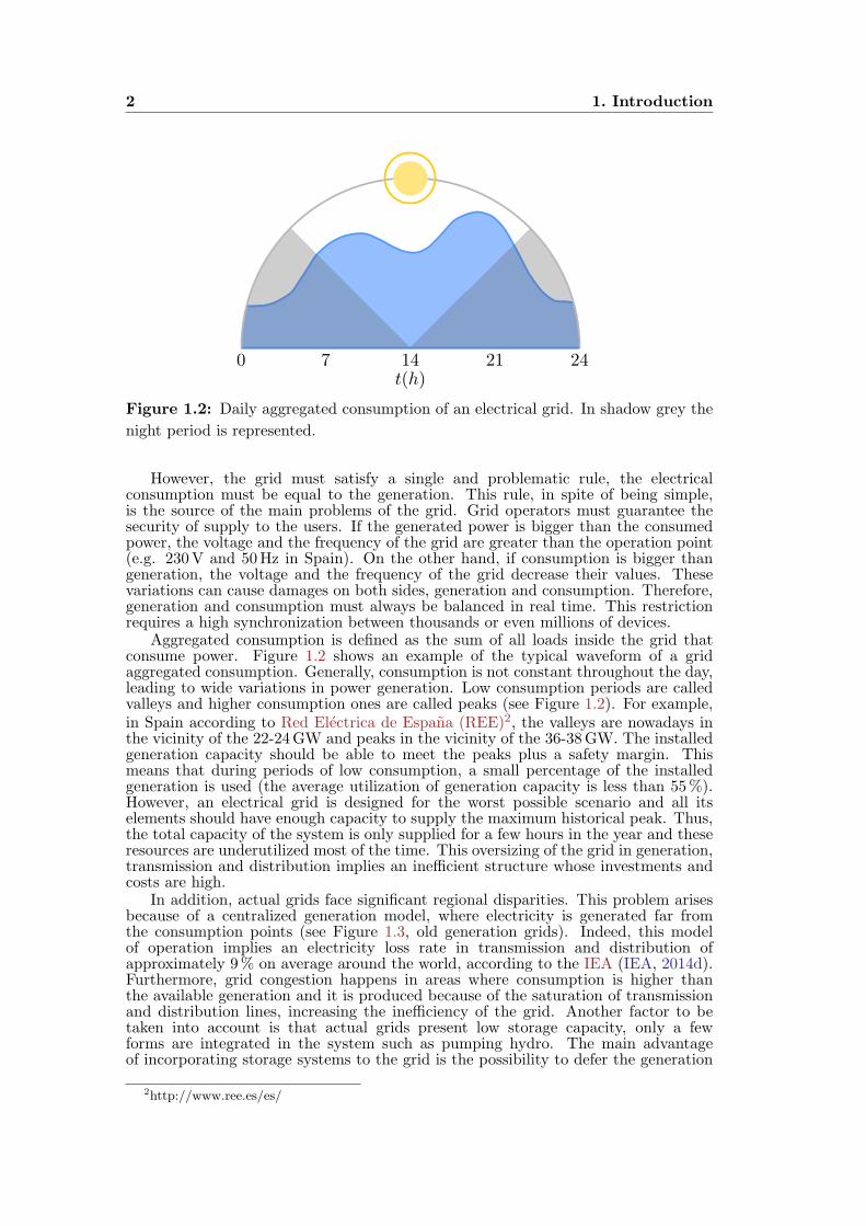
Figure 1.2: Daily aggregated consumption of an electrical grid. In shadow grey the
night period is represented.
However, the grid must satisfy a single and problematic rule, the electricalconsumption must be equal to the generation. This rule, in spite of being simple,is the source of the main problems of the grid. Grid operators must guarantee thesecurity of supply to the users. If the generated power is bigger than the consumedpower, the voltage and the frequency of the grid are greater than the operation point(e.g. 230V and 50Hz in Spain). On the other hand, if consumption is bigger thangeneration, the voltage and the frequency of the grid decrease their values. Thesevariations can cause damages on both sides, generation and consumption. Therefore,generation and consumption must always be balanced in real time. This restrictionrequires a high synchronization between thousands or even millions of devices.
Aggregated consumption is defined as the sum of all loads inside the grid thatconsume power. Figure 1.2 shows an example of the typical waveform of a gridaggregated consumption. Generally, consumption is not constant throughout the day,leading to wide variations in power generation. Low consumption periods are calledvalleys and higher consumption ones are called peaks (see Figure 1.2). For example,in Spain according to Red Electrica de Espana (REE)2, the valleys are nowadays inthe vicinity of the 22-24GW and peaks in the vicinity of the 36-38GW. The installedgeneration capacity should be able to meet the peaks plus a safety margin. Thismeans that during periods of low consumption, a small percentage of the installedgeneration is used (the average utilization of generation capacity is less than 55%).However, an electrical grid is designed for the worst possible scenario and all itselements should have enough capacity to supply the maximum historical peak. Thus,the total capacity of the system is only supplied for a few hours in the year and theseresources are underutilized most of the time. This oversizing of the grid in generation,transmission and distribution implies an inefficient structure whose investments andcosts are high.
In addition, actual grids face significant regional disparities. This problem arisesbecause of a centralized generation model, where electricity is generated far fromthe consumption points (see Figure 1.3, old generation grids). Indeed, this modelof operation implies an electricity loss rate in transmission and distribution ofapproximately 9% on average around the world, according to the IEA (IEA, 2014d).Furthermore, grid congestion happens in areas where consumption is higher thanthe available generation and it is produced because of the saturation of transmissionand distribution lines, increasing the inefficiency of the grid. Another factor to betaken into account is that actual grids present low storage capacity, only a fewforms are integrated in the system such as pumping hydro. The main advantageof incorporating storage systems to the grid is the possibility to defer the generation
2http://www.ree.es/es/
1.1. Motivation and Problem statement 3
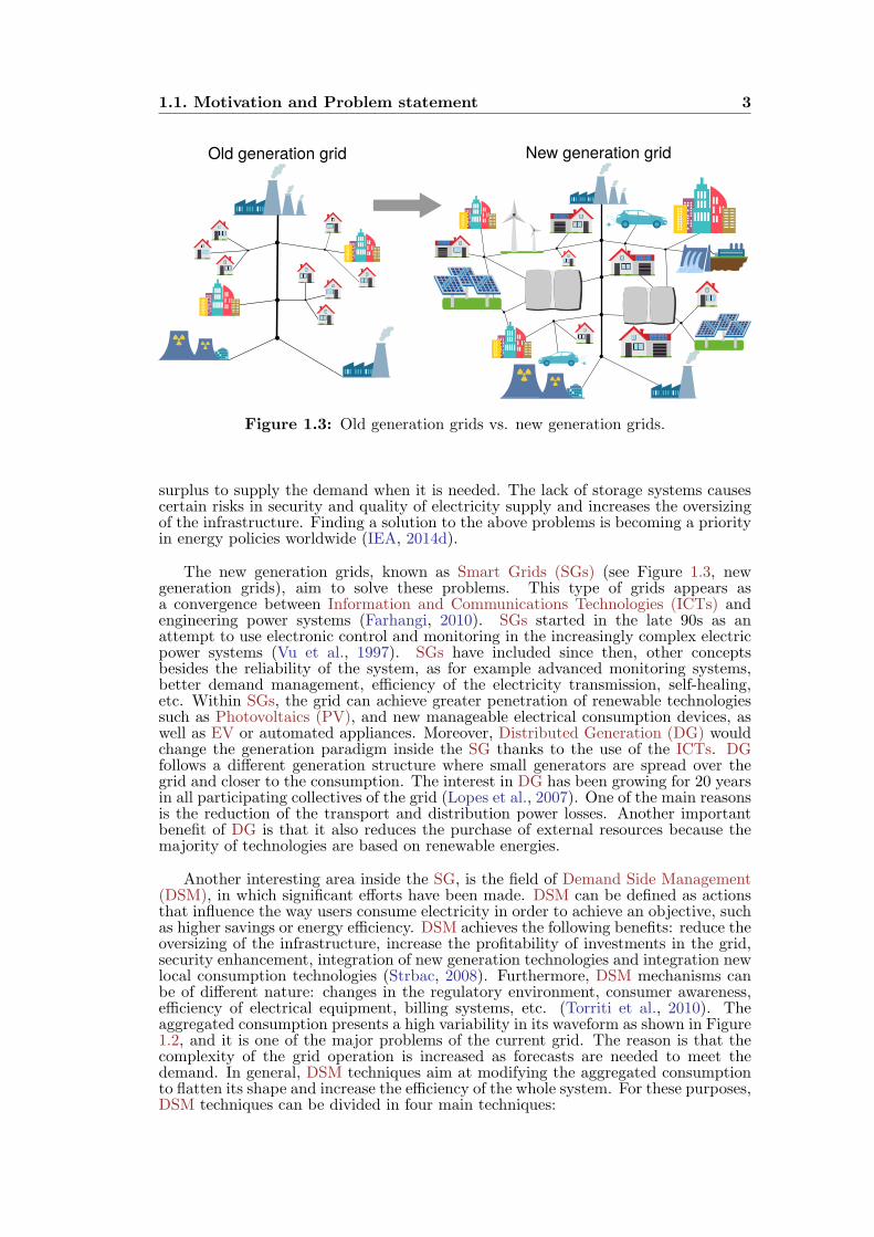
Old generation grid New generation grid
Figure 1.3: Old generation grids vs. new generation grids.
surplus to supply the demand when it is needed. The lack of storage systems causescertain risks in security and quality of electricity supply and increases the oversizingof the infrastructure. Finding a solution to the above problems is becoming a priorityin energy policies worldwide (IEA, 2014d).
The new generation grids, known as Smart Grids (SGs) (see Figure 1.3, newgeneration grids), aim to solve these problems. This type of grids appears asa convergence between Information and Communications Technologies (ICTs) andengineering power systems (Farhangi, 2010). SGs started in the late 90s as anattempt to use electronic control and monitoring in the increasingly complex electricpower systems (Vu et al., 1997). SGs have included since then, other conceptsbesides the reliability of the system, as for example advanced monitoring systems,better demand management, efficiency of the electricity transmission, self-healing,etc. Within SGs, the grid can achieve greater penetration of renewable technologiessuch as Photovoltaics (PV), and new manageable electrical consumption devices, aswell as EV or automated appliances. Moreover, Distributed Generation (DG) wouldchange the generation paradigm inside the SG thanks to the use of the ICTs. DGfollows a different generation structure where small generators are spread over thegrid and closer to the consumption. The interest in DG has been growing for 20 yearsin all participating collectives of the grid (Lopes et al., 2007). One of the main reasonsis the reduction of the transport and distribution power losses. Another importantbenefit of DG is that it also reduces the purchase of external resources because themajority of technologies are based on renewable energies.
Another interesting area inside the SG, is the field of Demand Side Management(DSM), in which significant efforts have been made. DSM can be defined as actionsthat influence the way users consume electricity in order to achieve an objective, suchas higher savings or energy efficiency. DSM achieves the following benefits: reduce theoversizing of the infrastructure, increase the profitability of investments in the grid,security enhancement, integration of new generation technologies and integration newlocal consumption technologies (Strbac, 2008). Furthermore, DSM mechanisms canbe of different nature: changes in the regulatory environment, consumer awareness,efficiency of electrical equipment, billing systems, etc. (Torriti et al., 2010). Theaggregated consumption presents a high variability in its waveform as shown in Figure1.2, and it is one of the major problems of the current grid. The reason is that thecomplexity of the grid operation is increased as forecasts are needed to meet thedemand. In general, DSM techniques aim at modifying the aggregated consumptionto flatten its shape and increase the efficiency of the whole system. For these purposes,DSM techniques can be divided in four main techniques:
4 1. Introduction
0 7 14 21 24t(h)
(a)
0 7 14 21 24t(h)
(b)
0 7 14 21 24t(h)
(c)
0 7 14 21 24t(h)
(d)
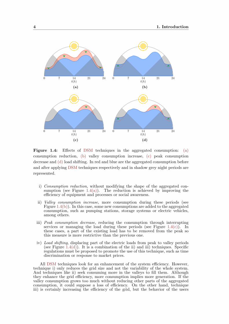
Figure 1.4: Effects of DSM techniques in the aggregated consumption: (a)
consumption reduction, (b) valley consumption increase, (c) peak consumption
decrease and (d) load shifting. In red and blue are the aggregated consumption before
and after applying DSM techniques respectively and in shadow grey night periods are
represented.
i) Consumption reduction, without modifying the shape of the aggregated con-sumption (see Figure 1.4(a)). The reduction is achieved by improving theefficiency of equipment and processes or social awareness.
ii) Valley consumption increase, more consumption during these periods (seeFigure 1.4(b)). In this case, some new consumptions are added to the aggregatedconsumption, such as pumping stations, storage systems or electric vehicles,among others.
iii) Peak consumption decrease, reducing the consumption through interruptingservices or managing the load during these periods (see Figure 1.4(c)). Inthese cases, a part of the existing load has to be removed from the peak sothis measure is more restrictive than the previous one.
iv) Load shifting, displacing part of the electric loads from peak to valley periods(see Figure 1.4(d)). It is a combination of the ii) and iii) techniques. Specificregulations must be proposed to promote the use of this technique, such as timediscrimination or response to market prices.
All DSM techniques look for an enhancement of the system efficiency. However,technique i) only reduces the grid size and not the variability of the whole system.And techniques like ii) seek consuming more in the valleys to fill them. Althoughthey enhance the grid efficiency, more consumption implies more generation. If thevalley consumption grows too much without reducing other parts of the aggregatedconsumption, it could suppose a loss of efficiency. On the other hand, techniqueiii) is certainly increasing the efficiency of the grid, but the behavior of the users
1.2. Thesis aim 5
is being restricted. Thus, for these reasons, technique iv) tries to compensate allthe disadvantages of previous techniques. Without adding more consumption to thesystem, it is able to reduce the variability of the aggregated consumption, consideringthe behavior of users without interrupting their supply and reducing the consumptionduring certain periods of time. Therefore, this last technique is emerging as animportant incentive to include in the development of SG since it helps to improvethe system’s operation and means a better integration of the different parts of thegrid.
In this Thesis, a solution to the aforementioned problems from an ArtificialIntelligence (AI) perspective is proposed. Specifically, it is proposed the use ofArtificial Neural Networks (ANNs) to manage the flows of energy inside the futureSG. The use of ANNs is motivated by the advantages of working with distributed,adaptive and nonlinear systems. Inside the field of ANN, Recurrent Neural Networks(RNNs) have been selected because of their dynamic behavior, which fits perfectlywith the non linear dynamic behavior of the grid. In addition, a neural controlleris developed to operate in each element of the grid, in order to increase its globalefficiency by smoothing the aggregated consumption. Inside this grid environment, itis also contained DG, particularly PV because it is the only renewable generationtechnology liable to be widely used in consumption points. Thus, the effects oflocal supply inside the grid and the penetration of PV without destabilizing thegrid behavior are studied. Finally, it is worthy to mention that the sole informationavailable from the grid is the aggregated consumption. The neural controllers makedecisions based on this sole information.
1.2 Thesis aim
The aim of this Thesis is the development of an adaptive algorithm to manage theconsumption of a collective of individuals with the presence of Distributed EnergyResources (DER), which combines the DG with storage systems. The objective ofthis algorithm is to enhance the efficiency of a grid by reducing the variability ofthe aggregated consumption through its smoothing. The only information availablefor the algorithm is the aggregated consumption coming from the grid. With thisinformation the algorithm must decide when it is the best time to consume aimingto accomplish the objective of smoothing the curve. Thus, the algorithm with thehistorical data of the grid has to predict and adapt the consumption of severalindividuals to fill the valley and decrease the peaks. As a whole, the collective ofindividuals must produce a flat aggregated consumption. Thus, the distributed self-organized algorithm senses the global behavior of a grid and only changes the localbehavior of each individual inside the collective. Therefore, this Thesis seeks fora distributed DSM approach combined with an automatic control of demand thathelps to integrate DER (DG and Electrical Energy Storage (EES)), which leads toan innovative concept called Active Demand Side Management (ADSM).
In addition, the grid is a highly non linear and dynamic system, due to the largenumber of elements and variables involved. For these reasons, ANNs have been chosento develop the algorithm. ANNs have a high ability to learn from the environment andall information is processed in a distributed manner (Haykin, 2009). More precisely,RNNs, a variant of ANNs, present the necessary features to model such a complexsystem. The use of these algorithms allows taking advantage of the RNN propertiessuch as non-linearity, adaptability, dynamics, distributivity, robustness, etc. Theseare enough advantages to develop an algorithm based on RNN.
From the energy efficiency point of view, the application of DSM techniques isable to enhance the grid performance. In this way, the oversizing of the grid andwaste of the existing resources inside the grid are avoided. In addition, it is becomingmore common to find DG inside grids because of the increase of solutions and theirbenefits. Hence, this Thesis seeks to take advantage of the energy resources availablelocally through PV DG. However, the local availability of electricity to supply thelocal demand could increase the variability of the aggregated consumption. Thisfact concerns to grid operators, who think that a high penetration of PV generation

6
could be detrimental to the grid stability. Therefore, this Thesis tries to solve the PVintegration problem, mitigating the stability grid issue and increasing the penetrationof this source of electricity.
In the design of the ADSM algorithm, the following features have been taken intoaccount:
Adaptivity, it has to react quickly to changes in the aggregated consumptionand adapt its output to counteract them.
System dynamics, the grid is a complex system to model, so that the algorithmhas to understand its nonlinear behavior over time by using the flows of energy,internal feedback loops and time delays.
Robustness, it has to tolerate perturbations that might affect its functioning orthe grid.
Distributed system, the algorithm operates locally at the individual level, butthe result of the whole should be flattened aggregated consumption withoutinteractions or passing information among them.
Scalability, it must be able to operate with any number of users inside thegrid. This implies that it has to allow the incorporation of new users withoutinterfering with its operation.
Data availability, due to the privacy of the users inside the grid, the onlyinformation available is the aggregated consumption and the local consumptionwhere it is operating. There is no information exchange among the individuals.This is a restriction due to the way that the data privacy is treated inside theactual grids.
1.3 Thesis structure
This Thesis is divided in three main parts. In Part I, the basic concepts of this Thesisare introduced to provide the reader with the necessary context to understand theproblem stated and the proposed solution. Chapter 2 gives an introduction to theenergy concepts related with the grid. The ANN concepts and description of theelements used to develop the ADSM algorithm are described in Chapter 3.
In Part II, the proposed ADSM algorithm is described. The development of thealgorithm has been divided in three different stages based on simplifications of thegrid environment. Chapter 4 proposed a first approximation of the problem basedon a reduced environment of two users, one controllable and one non-controllable.The neural controller parameters are tuned in order to solve this simplification of theproblem and an analysis of its performance is developed. Then, in Chapter 5, theproblem is taken to the next step and an algorithm is developed to coordinate theresponse of the neural controllers in a collective environment where the behavior ofcontrollable and non-controllable users is analyzed. Chapter 6 summarizes the resultsof using the proposed algorithm in a simulated grid environment.
The conclusions and future works are collected in Part III with Chapter 7. Section7.1 reviews the work done in the Thesis and discusses its main aspects. Section 7.2suggests a list of proposals and improvements of the proposed algorithms. Finally, areview of the author related contributions is summarized in Section 7.3.

PART I
Background

2Grid Framework
“All power corrupts, but we need the electricity” — Anonymous
Electricity has become an essential part of life. Like air, for most users it is atransparent fact in their lives, of which they have no notice. It is only whenpower disappears during a failure, when people realize how importantelectricity is in daily life. Electricity is used to power computers, mobile
phones, cooling, cooking, washing clothes, lights, entertainment, transportation, etc.(Brain and Roos, 2000). But, how is it possible that electricity is there when switchingon a light? How is electricity able to reach every place instantaneously? The answerto both questions is the electrical grid or only the “grid”. A grid is a network ofelectrical power systems which operates in real-time (Blume, 2007). This means thatpower is generated, transported and supplied in the same instant that it is needed.The main rule of the grid is that generation must match consumption. Electric powersystems do not inherently store energy such as water or gas systems. The reason isin the nature of electricity which is produced by the movement of electrons. Instead,generators produce the energy as the demand calls for it.
Thus, the grid is a vast physical and human network connecting thousands ofelectricity generators to millions of consumers — a linked system of public and privateenterprises operating. However, it had only minor changes in its structure for the pastcentury. So, the grid will face different challenges over the next decades, while newtechnologies arise as valuable opportunities to meet these challenges (MIT, 2011).Some of them are already here such as integration of renewable energy, DistributedGeneration (DG) or smart metering. If grid operators fail to realize about thesechallenges, it could result in degraded reliability, significantly increased costs, anda failure to achieve several public policy goals (MIT, 2011). To overcome thesedrawbacks, it is necessary to take the grid to the next level. The Smart Grid (SG)is conceived to address the global challenges of energy security, climate change andeconomic growth. SGs have some features that enable several low-carbon energytechnologies, including Electric Vehicles (EVs), variable renewable energy sourcesand Demand Side Management (DSM) (IEA, 2011).
In this Chapter, the current status of the electric system is introduced (seeSection 2.1), the main parts in which is divided, such as generation (Section2.1.1), transmission (Section 2.1.2), substations (Section 2.1.3), distribution (Section2.1.4) and consumption (Section 2.1.5). Thus, the present form of the grid isintroduced together with the identified issues that operators have to tackle withinthe evolution towards the next grid generation. These problems will be reportedin Section 2.2. After introducing all these concepts, explanations about what theSG is and the changes involved in its deployment, both structural (physical) andinternal (logical), are presented. Thus, in Section 2.3, the concept of the SG isdefined and the key aspects on which it is founded are introduced: Information andCommunications Technology (ICT) (see Section 2.3.1), DG (Section 2.3.2), ElectricalEnergy Storage (EES) (Section 2.3.3) and DSM (Section 2.3.4). In this Thesis, the useof DSM techniques are emphasized in order to enhance the grid efficiency integratingrenewable generation and EES. All of them are necessary for the proper growth of adevelopment environment and proper operation of these new generation power grids.

10 2. Grid Framework
2.1 The electric power systems
The electric power system is one of the most complex man-made systems. It consistsof a set of elements that operate coordinately in a territory to satisfy the demand. Thefirst electric power system was introduced in 1882 by Thomas Edison. It consistedof 59 customers connected in Direct Current (DC) at a price of about 5 $/kWh (MIT,2011). The development of the grid has been made over the last century and a half.Initially, the electric power systems supplied different, small and isolated consumers.And, the grid was born of the interconnection of these systems as a result of demandgrowth (Schewe, 2007). This interconnection was favored by two factors: i) thetransition from DC to Alternating Current (AC) power and ii) the use of transformersto elevate voltage, making transportation possible with fewer losses (MIT, 2011).AC power systems replaced DC ones because they present more advantages: easilyelevation of the voltage level and generators and motors are much simpler (Boyle,2007). During the next decades, new elements were introduced in the grids thatimproved the quality as consumption continued growing. With these achievementstogether with the growth of the grid, utilities could take advantage of economies ofscale and the price of electricity decreased its value.
Before the 1990s, individual companies controlled all the parts inside the gridfrom generation to delivery for a geographic area. In the 1990s, the regularization ofelectricity supplies changed, using markets rather than regulators to set prices, whereelectricity is treated as a commodity (Fox-Penner, 2010). Deregularization separatedthe generation into an industry apart and the electricity was produced far from theconsumers. This fact introduced more complexity and interconnectivity within thegrid. The more complex the grid becomes, the more instabilities affect the grid. Afailure in one part of the grid can be propagated to the remaining parts. Alongwith the aging of the infrastructure, power losses increased and maintaining them isincreasingly expensive.
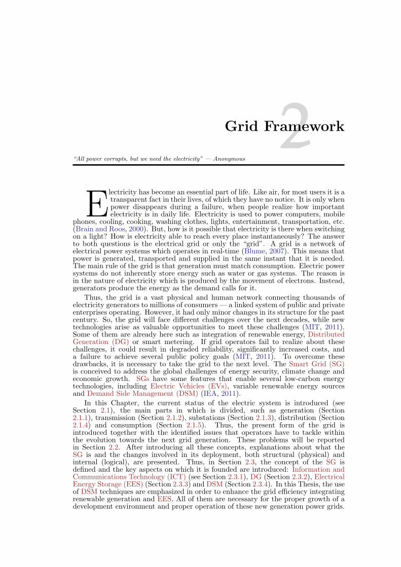
Despite the inclusion of new developments within the grid structure, it has notchanged its main internal organization in about a century and a half. Electrical gridsaround the world have a vertical structure, which interconnect generators, substations,transmission networks, distribution lines and consumption. Figure 2.1 shows the basicbuilding blocks of the grid, in which the different elements mentioned before are shown(Kirtley, 2010).
Generation is the part of the grid in charge of producing electricity. Thereare different types of generators that convert primary energy sources, such asfossil fuels and renewable resources, into electricity, e.g.: nuclear power plants,combined cycle plants, wind plants, Photovoltaics (PV) solar plants and hydropower plants among others. The size of the generators varies from few kilowattsof small diesel generators to thousands of megawatts of nuclear power plants.
Substations are in charge of conditioning the electricity power between elementsof the grid. These centers are responsible for raising or lowering the voltage(high/medium voltage and medium/low voltage) to couple different gridsections. Hence, they contain different elements such as transformers, electricalbuses, capacitor banks, etc. In addition, substations can operate in the gridthrough protective relaying, breaker controls, metering, etc.
Transmission network transports large amounts of electricity from generatorsto substations located close to the consumers. Almost every transmission line ishigh-voltage, three phases and AC. Electricity is transmitted at high voltages toreduce the energy losses over long distances. The electricity power parameters(voltage, frequency and number of phases) are regulated by the organ in chargeof managing the grid, usually at country level.
Distribution network transfers the electricity from the substations to itsdestination. The distribution lines operate at medium/low voltage depending onthe consumers requirements. For instance, the electricity could be distributed
2.1. The electric power systems 11
Generators
Transmission network
Industrial
consumer
Residential
consumer
Substation
Distribution network
Figure 2.1: Block diagram of an actual electrical grid.
in one or more phases (typically up to three phases). In addition, the electricitylines that reach homes provide generally a single phase of 230V in Europe.
Consumption is considered as the electrical energy used by all the elements insidethe power system. Thus, any device that transforms electric power into work isconsidered as consumption of the system. Consumption is made up of differentheterogeneous elements that are grouped according to the final behavior of thegrid users or consumers, e.g.: industrial, commercial or residential. Losses dueto different elements within the grid are also considered as consumption.
These basic elements are part of different power systems. On the other hand,the grid electrical signal mainly consists of three physical characteristics: i) current,ii) voltage and iii) frequency (Blume, 2007). The electric current (i) is the amountof electric charge that flows inside a conductor per unit of time. Its unit in theInternational System of Units (SI) is the ampere (A). The electric potential differenceor voltage (v) is the work applied to move electric charges between two points. In otherwords, it is the force that electrons need to move. Its unit of measurement in SI is thevolt (V). Frequency (f) is the number of times a signal is repeated in certain time.Its unit of measurement is Hertz or hertz (Hz). For example, Europe has a value of50Hz, while in North America it is used 60Hz. In the rest of the world, the frequencytakes one of these two values depending on the country. All of these parameters aremonitored by the grid operators to guarantee the stability of the electric system. Thegrid must always provide the required electricity that meets the varying demand.The reason is that electricity is consumed at the same time that it is generated. Animbalance between supply and demand will damage the stability and quality (voltageand frequency) of the power supply (IEC, 2011). But how are these parametersaffected by that mismatch? If demand is greater than generation, frequency andvoltage values fall while if generation is greater than demand, frequency and voltagerise. The grid must remain safe and be capable of withstanding a large variety ofdisturbances to guarantee a reliable service. For these reasons, grid operators designdifferent contingency plans and constant surveillance from control centers (Kunduret al., 1994). One of the most widespread measures to achieve the right balancebetween generation and consumption is making electricity demand forecasts. Withthese forecasts, power plants prepare their production programs for each of the dayhours to meet that demand (Boyle, 2007).
In spite of being very dependable from the geographical area where the grids arebuilt, they present some features in common:
Ageing system, since the deployment of the electric grids, there have been nodeep changes in their infrastructure. It is not enough with this feature to meetthe needs of users as well as complicate the entry of new elements within thegrid. Therefore, it is necessary that the grid evolves at the same time that usersincrease their demands and technological evolution brings to the market newgeneration technologies.
Large scale. The grid must be able to supply different number of users, rangingfrom just a few to millions, depending on the size of the area to cover. This fact
12 2. Grid Framework
IE
NI
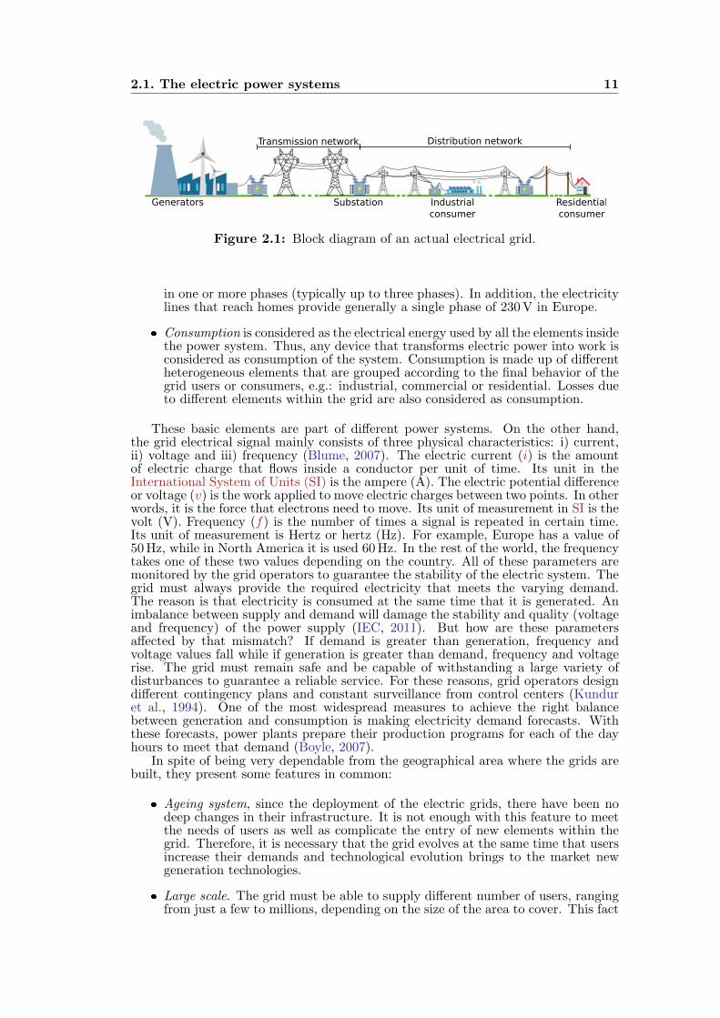
-W
Figure 2.2: Map of electric exchanges for the different European countries. The
thickness of the different arrows represents the amount of power exchanged between
the different European countries.
raises the serious problem of avoiding potential performance degradation as thegrid size increases.
Geographical distribution. The grid is deployed along the length of the differentcountries where it is installed, covering most of the population. There may beone or more operators responsible for supplying the demand. These operatorsinstall the elements to guarantee the access to electricity, power lines, controlcenters, substations, etc.
Interconnected power systems. The interconnection among electric systemsallows guaranteeing the supply in a given territory when a particular systemcannot generate enough power to meet demand. This happens when extraor-dinary and unexpected consumptions occur (e.g. a cold snap), or when oneor several generation centers are no longer operating temporarily and enoughelectricity is not injected into the system. For this reason, the more electricalsystems are interconnected and the higher the capacity of energy exchanged is,the greater the safety and quality of service they provide. For example, thecontinental European electricity system is connected to the Nordic countriesand the British Isles by North and Eastern countries (see Figure 2.2).
Heterogeneity. A grid hosts elements whose nature is very different. Within thegrid there are different generators types, different power lines, different types ofconsumers, etc. There are also differences between the physical features of theelectricity supplied, different frequencies (50Hz or 60Hz) or different voltage
2.1. The electric power systems 13
(120V or 230V). The values of these parameters depend on the region in whichthe grid is located.
One-way communication. Consumers are mostly uninformed and do not haveactive part in the system, they only demand electricity. The communicationgoes therefore from generators to consumers through control centres of the gridoperators. However, if users get involved in the process, the efficiency of thesystem would be enhanced. The reason is that their behaviour affects directlyto the grid status and the modifications of this behavior increases the gridoperation effectiveness.
Multiple agents. Each grid may establish different security and administrativepolicies under which a safe electricity market can be developed and would beprofitable for all participants. As a result, the already challenging grid securityproblem is complicated even more with the inclusion of new communicationtechnologies.
Resource coordination. Resources in a grid must be coordinated in order toprovide aggregated capabilities. Thus, the generation could meet the demandat any time without any problem.
Access to the grid must be: i) transparent, the grid should be seen as a singlesystem, ii) reliable, the grid must guarantee the supply to the users at anymoment under established quality of services requirements, iii) consistent, thegrid must bring together all its constituent elements to supply the demand,and iv) universal, the grid must grant access throughout the whole operationterritory and adapt itself to a dynamic environment that changes continuously.
Nowadays, the integration of new generation technologies into the grid is becomingcomplex due to its age. New technologies powered by renewable resources such aswind and solar energy are increasingly becoming part of the generation mixturewith considerable difficulties because of the variability of these energy resources(Boyle, 2007) and the centralized generation paradigm on which electric grids arebased. In order to include these resources, it is necessary to use sophisticatedmanagement algorithms that can meet the demand in real-time. Thus, the algorithmsare constantly changing the supplies of energy from different sources to tackle thevariability of renewable energies. Collecting data from the different elements of thegrid could help to perform the complex calculations for grid stabilization. On theother hand, a bad management of the collected data supposes a curse to the system.It is in this scenario in which the SG arises. The concept of the SG will be explainedlater in Section 2.3. But first, each grid component is explained in more detail.
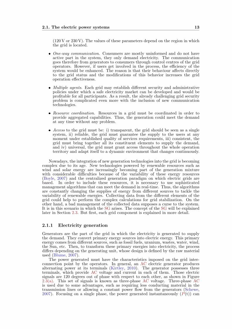
2.1.1 Electricity generation
Generators are the part of the grid in which the electricity is generated to supplythe demand. They convert primary energy sources into electric energy. This primaryenergy comes from different sources, such as fossil fuels, uranium, wastes, water, wind,the Sun, etc. Then, to transform these primary energies into electricity, the processdiffers depending on the generating unit, whose design is defined by the raw materialused (Blume, 2007).
The power generated must have the characteristics imposed on the grid inter-connection point by the operators. In general, an AC electric generator producesalternating power at its terminals (Kirtley, 2010). The generator possesses threeterminals, which provide AC voltage and current in each of them. Those electricsignals are 120 degrees out of phase with respect to each other, as shown in Figure2.3(a). This set of signals is known as three-phase AC voltage. Three-phase ACis used due to some advantages, such as requiring less conducting material in thetransmission lines or allowing a constant power flow from the generators (Schewe,2007). Focusing on a single phase, the power generated instantaneously (P (t)) can
14 2. Grid Framework
Phase 1 Phase 2Phase 3
t
V (t)
(a)
S Q P P(t)
V(t) I(t)
t
(b)
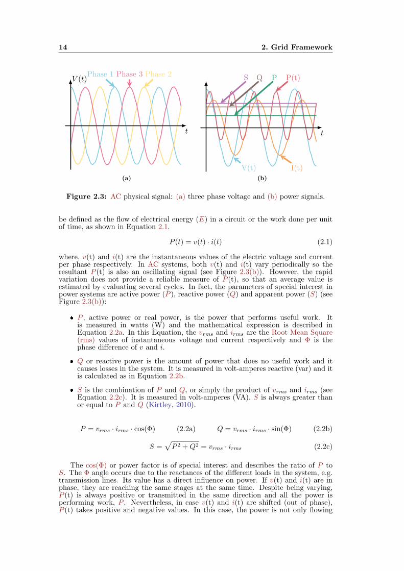
Figure 2.3: AC physical signal: (a) three phase voltage and (b) power signals.
be defined as the flow of electrical energy (E) in a circuit or the work done per unitof time, as shown in Equation 2.1.
P (t) = v(t) · i(t) (2.1)
where, v(t) and i(t) are the instantaneous values of the electric voltage and currentper phase respectively. In AC systems, both v(t) and i(t) vary periodically so theresultant P (t) is also an oscillating signal (see Figure 2.3(b)). However, the rapidvariation does not provide a reliable measure of P (t), so that an average value isestimated by evaluating several cycles. In fact, the parameters of special interest inpower systems are active power (P ), reactive power (Q) and apparent power (S) (seeFigure 2.3(b)):
P , active power or real power, is the power that performs useful work. Itis measured in watts (W) and the mathematical expression is described inEquation 2.2a. In this Equation, the vrms and irms are the Root Mean Square(rms) values of instantaneous voltage and current respectively and Φ is thephase difference of v and i.
Q or reactive power is the amount of power that does no useful work and itcauses losses in the system. It is measured in volt-amperes reactive (var) and itis calculated as in Equation 2.2b.
S is the combination of P and Q, or simply the product of vrms and irms (seeEquation 2.2c). It is measured in volt-amperes (VA). S is always greater thanor equal to P and Q (Kirtley, 2010).
P = vrms · irms · cos(Φ) (2.2a) Q = vrms · irms · sin(Φ) (2.2b)
S =√
P 2 +Q2 = vrms · irms (2.2c)
The cos(Φ) or power factor is of special interest and describes the ratio of P toS. The Φ angle occurs due to the reactances of the different loads in the system, e.g.transmission lines. Its value has a direct influence on power. If v(t) and i(t) are inphase, they are reaching the same stages at the same time. Despite being varying,P (t) is always positive or transmitted in the same direction and all the power isperforming work, P . Nevertheless, in case v(t) and i(t) are shifted (out of phase),P (t) takes positive and negative values. In this case, the power is not only flowing

2.1. The electric power systems 15
Nuclear
Thermal:
– Coal
– Fuel
– Gas
Biomass
Cogeneration
Solar thermal
Hydro
Wind
Photovoltaics
Heat to
evaporate
waterTurbine
connected
to
generator
Electricity
to the grid
Figure 2.4: Forms of electricity generation.
in one direction (P ), there is also a back and forth movement (Q). The sign of P (t)indicates its direction, but for P and Q, the sign indicates the phase shift of v(t)and i(t). Because Q produces no useful work, power systems try to compensate Φby using specific loads to correct this behavior. Grid operators want a cos(Φ)= 1,because it implies that all the generated power is performing useful work (von Meier,2006).
In order to generate electricity, the most widespread method consists of trans-forming mechanical energy in electricity through the movement of a turbine. That isthe reason why electricity is normally called a secondary energy source. A turbine isa simple device with few parts that uses flowing fluids (liquids or gases), forcing themto pass through blades mounted on a shaft, which causes the shaft to turn. Then,the mechanical energy produced from the rotation of the shaft is collected by anAC electric generator which converts the motion to electricity by means of magneticfields (von Meier, 2006). There are three main sources to supply a generator withmechanical energy: i) high pressure steam, ii) falling liquid water and iii) wind. Figure2.4 shows the principal forms of generating electricity. Except for PV generators therest of them include a turbine and a generator. So, different power plants can alsobe classified depending on the turbine used to transform the primary energy used(Blume, 2007):
Steam turbine, it uses high-pressure and high-temperature steam to drive themechanical shaft of the AC electric generator. The steam is created in a boiler,furnace, or heat exchanger and moved to the turbine. Depending on the fuel,there exist different power plants. Examples of power plants that uses steamturbine are nuclear, thermal, geothermal, solar-thermal and biomass, amongothers.
Hydro turbine, it takes advantage of the water to generate electricity. Hydroelec-tric power plants convert the kinetic energy of falling water under the influenceof gravity.
Combustion turbine power plants burn fuel in a jet engine and use the exhaustgasses to spin a turbine generator. In general, it uses a mixture of a fuel (e.g.,diesel fuel, jet fuel, or natural gas) and air. The power plants that use this typeof turbine are known as combined-cycle power plant.
16 2. Grid Framework
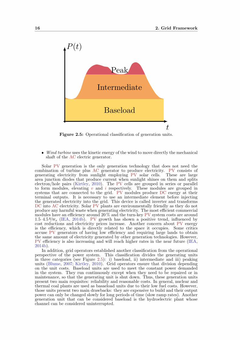
Baseload
Intermediate
Peak
t
P (t)
Figure 2.5: Operational classification of generation units.
Wind turbine uses the kinetic energy of the wind to move directly the mechanicalshaft of the AC electric generator.
Solar PV generation is the only generation technology that does not need thecombination of turbine plus AC generator to produce electricity. PV consists ofgenerating electricity from sunlight employing PV solar cells. These are largearea junction diodes that produce current when sunlight shines on them and splitselectron/hole pairs (Kirtley, 2010). The PV cells are grouped in series or parallelto form modules, elevating v and i respectively. These modules are grouped insystems that are connected to the grid. PV modules produce DC energy at theirterminal outputs. It is necessary to use an intermediate element before injectingthe generated electricity into the grid. This device is called inverter and transformsDC into AC electricity. Solar PV plants are environmentally friendly as they do notproduce any harmful waste when generating electricity. The most efficient commercialmodules have an efficiency around 20% and the turn-key PV system costs are around1.5–4.5 $/Wp (IEA, 2014b). PV growth has shown a positive trend, influenced bycost reductions and electricity prices increase. Another concern about PV energyis the efficiency, which is directly related to the space it occupies. Some criticsaccuse PV generators of having low efficiency and requiring large lands to obtainthe same amount of electricity generated by other generation technologies. However,PV efficiency is also increasing and will reach higher rates in the near future (IEA,2014b).
In addition, grid operators established another classification from the operationalperspective of the power system. This classification divides the generating unitsin three categories (see Figure 2.5): i) baseload, ii) intermediate and iii) peakingunits (Blume, 2007; Kirtley, 2010). Grid operators ensure that division dependingon the unit costs. Baseload units are used to meet the constant power demandedin the system. They run continuously except when they need to be repaired or inmaintenance, so that the generating unit is shut down. Thus, these generation unitspresent two main requisites: reliability and reasonable costs. In general, nuclear andthermal coal plants are used as basaeload units due to their low fuel costs. However,those units present two main drawbacks: they are expensive to build and their outputpower can only be changed slowly for long periods of time (slow ramp rates). Anothergeneration unit that can be considered baseload is the hydroelectric plant whosechannel can be considered uninterrupted.
2.1. The electric power systems 17
The intermediate units are also called cycling units. The output power of theseunits is regulated depending on the time of the day and it is extended for longperiods of time. One feature that distinguishes this type of generation from baseloadgeneration is the ability to vary their output power faster. Combined-cycle gas turbineplants and thermal generating units generally are used as intermediate units. Finally,peaking units only generate when the demand is close to the maximum or peak ofthe power system. They run only for a few hours per day, so they have to be ableto start and stop quickly. Combined-cycle gas turbine and hydroelectric plants withreservoirs are generally used as peaking units. Combined-cycle gas turbines are theleast expensive to build but have high operating costs.
In general, large generating units are located far from where their power isconsumed, and the generated power has to be transported to load centers (Schewe,2007). In order to reduce power losses during transmission, the generation voltageis raised from tens of kV to a few hundred using a transformer. Grid operators areconstantly watching that generating units are synchronized (Kundur et al., 1994).Apart from large generating systems inside the grid, there exist also some smallscale distributed generators, including combined heat and power units. Inside thissmall generating units, small hydroelectric plants, solar PV systems or small windpower generators are found. They operate at lower voltages and are connected atthe distribution system level (Fox-Penner, 2010). Once explained the different formsof generation, it is necessary to transport this generated electricity to meet the userdemand.
2.1.2 The transmission system
The transmission system is the part of the grid in charge of transporting electricityover long distances, from the place where it is generated to the distribution network.Recently, the generation is getting closer to the places where it is demanded. However,it is still far from the consumers. Furthermore, the transmission network ensures thatthe generated power comes with the least possible losses. This network is composedof different elements i) power lines, ii) high towers and iii) substations. The powerlines are attached to the towers, which cover great lengths to fulfill their mission.However, insulated cables are normally used and buried underground when the powerlines have to go through a population. Substations are in charge of conditioning thepower transmitted and routing the power to its destination (see Section 2.1.3).
Different factors influence the transmission lines characteristics, such as current,material type, section, size, etc. These features will influence the amount of powerthat the line can transport inside it. The power line conductor presents a resistance(R) to the flow of current due to the properties of the material. This R makes theconductor to heat up, losing part of the transmitted power that circulates inside it.The conductor R is not constant with the length and it also varies with the diametersize of the conductor, being smaller the greater the diameter is (Blume, 2007). Thereare other effects present in the line due to the current. The flow of current throughthe line length produces magnetic fields which cause the appearance of an inductance(L) in series with the terminals of the line. Furthermore, a capacitance (C) appearsin parallel to the transmission line terminals due to the appearance of electric fieldsfor carrying voltage. Both, L and C depend on the power line length, the higherthe length is, the higher the value of the parameters is (Kirtley, 2010). These threeparameters, among others effects, are responsible for the losses in transmission lines.So it is very important to design properly the power lines to ensure the minimumlosses in the power transmission. Some aspects to take into account in their designare: i) material, ii) conductor configuration, iii) section and iv) length (Molburg et al.,2007; Blume, 2007; Kirtley, 2010).
The transmission network has to transport power over long distances, so thatHigh Voltage (HV) is used to reduce the losses. This transmission form reducesthe conductor cross-sectional area and requires less right-of-ways for a given power(Blume, 2007). Transmission losses are mainly due to heat radiation by the conductorswhen the current flows inside. Thus, remembering Equation 2.1, the same amount ofpower could be transported if v is increased while i is decreased. In consequence, the
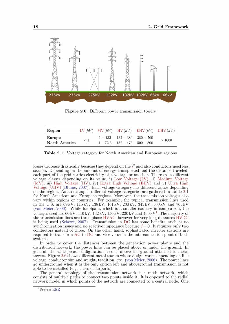
18 2. Grid Framework
275kV 275kV 275kV 132kV 132kV 132kV 66kV 66kV
Figure 2.6: Different power transmission towers.
Region LV (kV ) MV (kV ) HV (kV ) EHV (kV ) UHV (kV )
Europe< 1
1− 132 132− 380 380− 700> 1000
North America 1− 72.5 132− 475 500− 800
Table 2.1: Voltage category for North American and European regions.
losses decrease drastically because they depend on the i2 and also conductors need lesssection. Depending on the amount of energy transported and the distance traveled,each part of the grid carries electricity at a voltage or another. There exist differentvoltage classes depending on its value, i) Low Voltage (LV), ii) Medium Voltage(MV), iii) High Voltage (HV), iv) Extra High Voltage (EHV) and v) Ultra HighVoltage (UHV) (Blume, 2007). Each voltage category has different values dependingon the region. As an example, different voltage categories are gathered in Table 2.1for North American and European regions. Moreover, the transmission voltages alsovary within regions or countries. For example, the typical transmission lines usedin the U.S. are 69 kV, 115 kV, 138 kV, 161 kV, 230 kV, 345 kV, 500 kV and 765 kV(von Meier, 2006). While for Spain, which is a smaller country in comparison, thevoltages used are 60 kV, 110 kV, 132 kV, 150 kV, 220 kV and 400 kV1. The majority ofthe transmission lines are three phase HVAC, however for very long distances HVDCis being used (Schewe, 2007). Transmission in DC has some benefits, such as nosynchronization issues and no reactive impedance because f= 0. It requires only twoconductors instead of three. On the other hand, sophisticated inverter stations arerequired to transform AC to DC and vice versa in the interconnection point of bothsystems.
In order to cover the distances between the generation power plants and thedistribution network, the power lines can be placed above or under the ground. Ingeneral, the widespread configuration used is above the ground attached to metaltowers. Figure 2.6 shows different metal towers whose design varies depending on linevoltage, conductor size and weight, tradition, etc. (von Meier, 2006). The power linesgo underground when it is the only option left and aboveground transmission is notable to be installed (e.g. cities or airports).
The general topology of the transmission network is a mesh network, whichconsists of multiple paths to connect two points inside it. It is opposed to the radialnetwork model in which points of the network are connected to a central node. One
1Source: REE
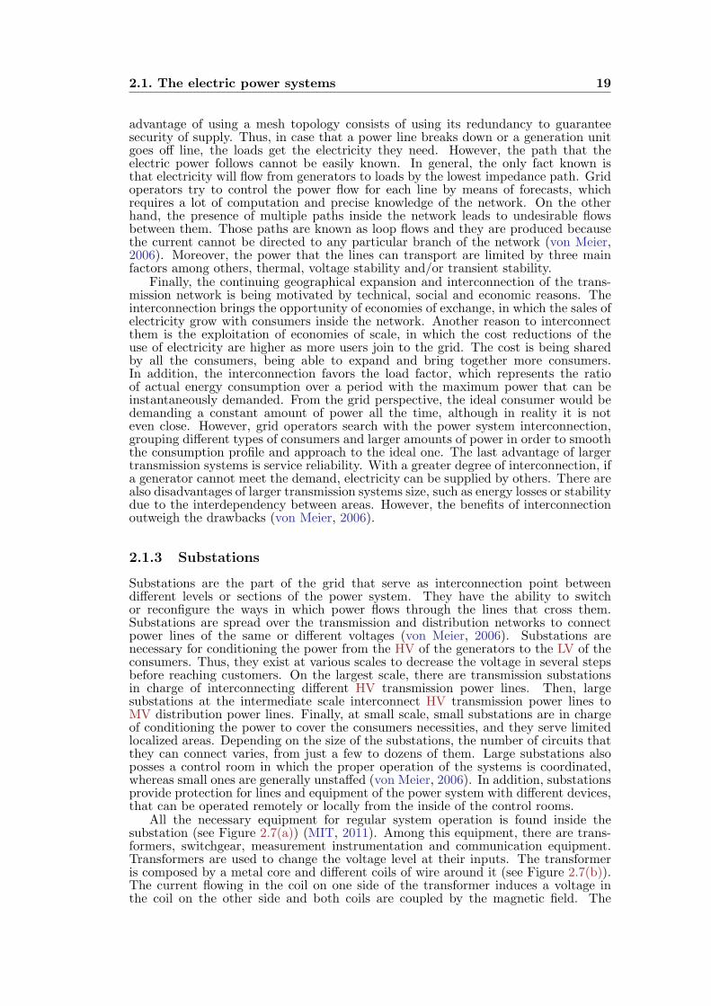
2.1. The electric power systems 19
advantage of using a mesh topology consists of using its redundancy to guaranteesecurity of supply. Thus, in case that a power line breaks down or a generation unitgoes off line, the loads get the electricity they need. However, the path that theelectric power follows cannot be easily known. In general, the only fact known isthat electricity will flow from generators to loads by the lowest impedance path. Gridoperators try to control the power flow for each line by means of forecasts, whichrequires a lot of computation and precise knowledge of the network. On the otherhand, the presence of multiple paths inside the network leads to undesirable flowsbetween them. Those paths are known as loop flows and they are produced becausethe current cannot be directed to any particular branch of the network (von Meier,2006). Moreover, the power that the lines can transport are limited by three mainfactors among others, thermal, voltage stability and/or transient stability.
Finally, the continuing geographical expansion and interconnection of the trans-mission network is being motivated by technical, social and economic reasons. Theinterconnection brings the opportunity of economies of exchange, in which the sales ofelectricity grow with consumers inside the network. Another reason to interconnectthem is the exploitation of economies of scale, in which the cost reductions of theuse of electricity are higher as more users join to the grid. The cost is being sharedby all the consumers, being able to expand and bring together more consumers.In addition, the interconnection favors the load factor, which represents the ratioof actual energy consumption over a period with the maximum power that can beinstantaneously demanded. From the grid perspective, the ideal consumer would bedemanding a constant amount of power all the time, although in reality it is noteven close. However, grid operators search with the power system interconnection,grouping different types of consumers and larger amounts of power in order to smooththe consumption profile and approach to the ideal one. The last advantage of largertransmission systems is service reliability. With a greater degree of interconnection, ifa generator cannot meet the demand, electricity can be supplied by others. There arealso disadvantages of larger transmission systems size, such as energy losses or stabilitydue to the interdependency between areas. However, the benefits of interconnectionoutweigh the drawbacks (von Meier, 2006).
2.1.3 Substations
Substations are the part of the grid that serve as interconnection point betweendifferent levels or sections of the power system. They have the ability to switchor reconfigure the ways in which power flows through the lines that cross them.Substations are spread over the transmission and distribution networks to connectpower lines of the same or different voltages (von Meier, 2006). Substations arenecessary for conditioning the power from the HV of the generators to the LV of theconsumers. Thus, they exist at various scales to decrease the voltage in several stepsbefore reaching customers. On the largest scale, there are transmission substationsin charge of interconnecting different HV transmission power lines. Then, largesubstations at the intermediate scale interconnect HV transmission power lines toMV distribution power lines. Finally, at small scale, small substations are in chargeof conditioning the power to cover the consumers necessities, and they serve limitedlocalized areas. Depending on the size of the substations, the number of circuits thatthey can connect varies, from just a few to dozens of them. Large substations alsoposses a control room in which the proper operation of the systems is coordinated,whereas small ones are generally unstaffed (von Meier, 2006). In addition, substationsprovide protection for lines and equipment of the power system with different devices,that can be operated remotely or locally from the inside of the control rooms.
All the necessary equipment for regular system operation is found inside thesubstation (see Figure 2.7(a)) (MIT, 2011). Among this equipment, there are trans-formers, switchgear, measurement instrumentation and communication equipment.Transformers are used to change the voltage level at their inputs. The transformeris composed by a metal core and different coils of wire around it (see Figure 2.7(b)).The current flowing in the coil on one side of the transformer induces a voltage inthe coil on the other side and both coils are coupled by the magnetic field. The
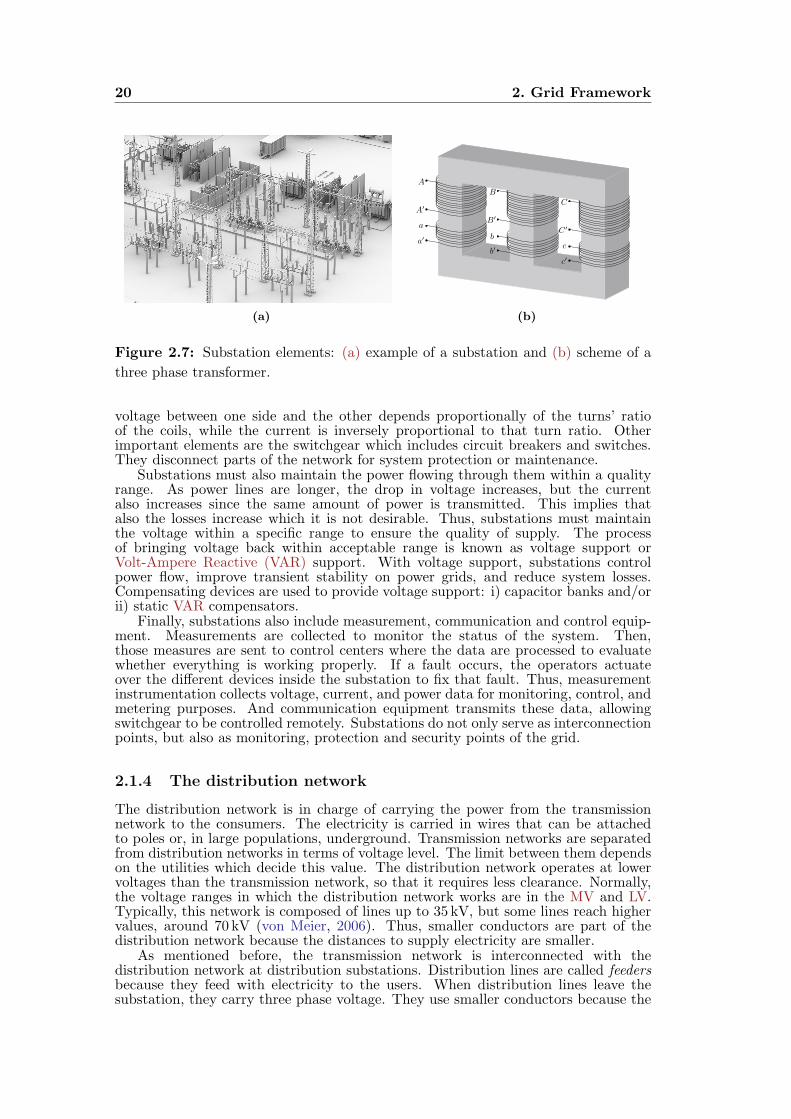
20 2. Grid Framework
(a)
A
A′
B
B′
C
C ′a
a′b
b′c
c′
(b)
Figure 2.7: Substation elements: (a) example of a substation and (b) scheme of a
three phase transformer.
voltage between one side and the other depends proportionally of the turns’ ratioof the coils, while the current is inversely proportional to that turn ratio. Otherimportant elements are the switchgear which includes circuit breakers and switches.They disconnect parts of the network for system protection or maintenance.
Substations must also maintain the power flowing through them within a qualityrange. As power lines are longer, the drop in voltage increases, but the currentalso increases since the same amount of power is transmitted. This implies thatalso the losses increase which it is not desirable. Thus, substations must maintainthe voltage within a specific range to ensure the quality of supply. The processof bringing voltage back within acceptable range is known as voltage support orVolt-Ampere Reactive (VAR) support. With voltage support, substations controlpower flow, improve transient stability on power grids, and reduce system losses.Compensating devices are used to provide voltage support: i) capacitor banks and/orii) static VAR compensators.
Finally, substations also include measurement, communication and control equip-ment. Measurements are collected to monitor the status of the system. Then,those measures are sent to control centers where the data are processed to evaluatewhether everything is working properly. If a fault occurs, the operators actuateover the different devices inside the substation to fix that fault. Thus, measurementinstrumentation collects voltage, current, and power data for monitoring, control, andmetering purposes. And communication equipment transmits these data, allowingswitchgear to be controlled remotely. Substations do not only serve as interconnectionpoints, but also as monitoring, protection and security points of the grid.
2.1.4 The distribution network
The distribution network is in charge of carrying the power from the transmissionnetwork to the consumers. The electricity is carried in wires that can be attachedto poles or, in large populations, underground. Transmission networks are separatedfrom distribution networks in terms of voltage level. The limit between them dependson the utilities which decide this value. The distribution network operates at lowervoltages than the transmission network, so that it requires less clearance. Normally,the voltage ranges in which the distribution network works are in the MV and LV.Typically, this network is composed of lines up to 35 kV, but some lines reach highervalues, around 70 kV (von Meier, 2006). Thus, smaller conductors are part of thedistribution network because the distances to supply electricity are smaller.
As mentioned before, the transmission network is interconnected with thedistribution network at distribution substations. Distribution lines are called feedersbecause they feed with electricity to the users. When distribution lines leave thesubstation, they carry three phase voltage. They use smaller conductors because the
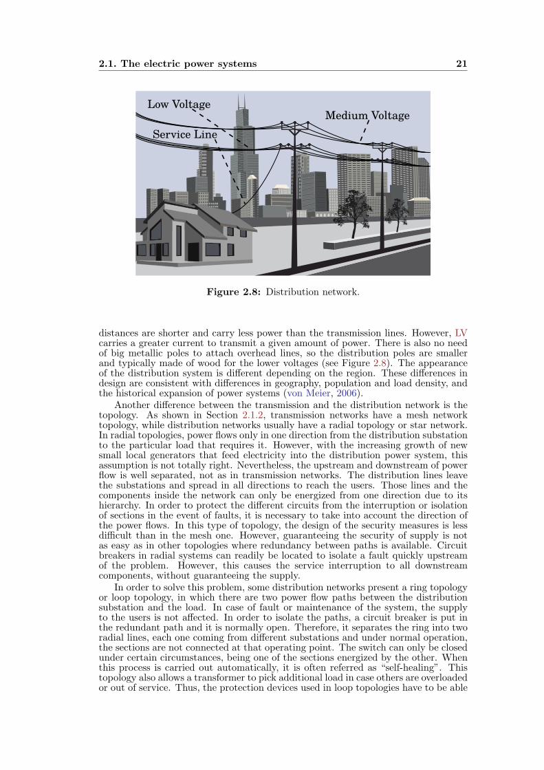
2.1. The electric power systems 21
Medium VoltageLow Voltage
Service Line
Figure 2.8: Distribution network.
distances are shorter and carry less power than the transmission lines. However, LVcarries a greater current to transmit a given amount of power. There is also no needof big metallic poles to attach overhead lines, so the distribution poles are smallerand typically made of wood for the lower voltages (see Figure 2.8). The appearanceof the distribution system is different depending on the region. These differences indesign are consistent with differences in geography, population and load density, andthe historical expansion of power systems (von Meier, 2006).
Another difference between the transmission and the distribution network is thetopology. As shown in Section 2.1.2, transmission networks have a mesh networktopology, while distribution networks usually have a radial topology or star network.In radial topologies, power flows only in one direction from the distribution substationto the particular load that requires it. However, with the increasing growth of newsmall local generators that feed electricity into the distribution power system, thisassumption is not totally right. Nevertheless, the upstream and downstream of powerflow is well separated, not as in transmission networks. The distribution lines leavethe substations and spread in all directions to reach the users. Those lines and thecomponents inside the network can only be energized from one direction due to itshierarchy. In order to protect the different circuits from the interruption or isolationof sections in the event of faults, it is necessary to take into account the direction ofthe power flows. In this type of topology, the design of the security measures is lessdifficult than in the mesh one. However, guaranteeing the security of supply is notas easy as in other topologies where redundancy between paths is available. Circuitbreakers in radial systems can readily be located to isolate a fault quickly upstreamof the problem. However, this causes the service interruption to all downstreamcomponents, without guaranteeing the supply.
In order to solve this problem, some distribution networks present a ring topologyor loop topology, in which there are two power flow paths between the distributionsubstation and the load. In case of fault or maintenance of the system, the supplyto the users is not affected. In order to isolate the paths, a circuit breaker is put inthe redundant path and it is normally open. Therefore, it separates the ring into tworadial lines, each one coming from different substations and under normal operation,the sections are not connected at that operating point. The switch can only be closedunder certain circumstances, being one of the sections energized by the other. Whenthis process is carried out automatically, it is often referred as “self-healing”. Thistopology also allows a transformer to pick additional load in case others are overloadedor out of service. Thus, the protection devices used in loop topologies have to be able
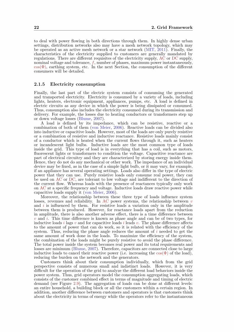
22 2. Grid Framework
to deal with power flowing in both directions through them. In highly dense urbansettings, distribution networks also may have a mesh network topology, which maybe operated as an active mesh network or a star network (MIT, 2011). Finally, thecharacteristics of the electricity supplied to customers are generally mandated byregulations. There are different requisites of the electricity supply, AC or DC supply,nominal voltage and tolerance, f , number of phases, maximum power instantaneously,cos(Φ), earthing system, etc. In the next Section, the consumption of the differentconsumers will be detailed.
2.1.5 Electricity consumption
Finally, the last part of the electric system consists of consuming the generatedand transported electricity. Electricity is consumed by a variety of loads, includinglights, heaters, electronic equipment, appliances, pumps, etc. A load is defined inelectric circuits as any device in which the power is being dissipated or consumed.Thus, consumption also includes the electricity consumed during its transmission anddelivery. For example, the losses due to heating conductors or transformers step upor down voltage losses (Blume, 2007).
A load is defined by its impedance, which can be resistive, reactive or acombination of both of them (von Meier, 2006). Reactive loads can be divided alsointo inductive or capacitive loads. However, most of the loads are only purely resistiveor a combination of resistive and inductive reactance. Resistive loads mainly consistof a conductor which is heated when the current flows through it, such as heatersor incandescent light bulbs. Inductive loads are the most common type of loadsinside the grid. This type of load is in everything that has a coil, such as motors,fluorescent lights or transformers to condition the voltage. Capacitive reactance arepart of electrical circuitry and they are characterized by storing energy inside them.Hence, they do not do any mechanical or other work. The impedance of an individualdevice may be fixed, as in the case of a simple light bulb, or it may vary, for example,if an appliance has several operating settings. Loads also differ in the type of electricpower that they can use. Purely resistive loads only consume real power, they canbe used on AC or DC, are tolerant to low voltage and indifferent to the direction ofthe current flow. Whereas loads with the presence of reactances typically only workon AC at a specific frequency and voltage. Inductive loads draw reactive power whilecapacitive loads supply it (von Meier, 2006).
Moreover, the relationship between these three type of loads influence systemlosses, revenues and reliability. In AC power systems, the relationship between vand i is influenced by them. For resistive loads a variation only in the amplitudebetween them is produced. However, for reactance loads apart from the reductionin amplitude, there is also another adverse effect, there is a time difference betweenv and i. This time difference is known as phase angle and can be of two types, forinductive loads i lags v and for capacitive loads i leads v. The phase difference affectsto the amount of power that can do work, so it is related with the efficiency of thesystem. Thus, reducing the phase angle reduces the amount of i needed to get thesame amount of work done in the loads. To maximize the efficiency of the system,the combination of the loads might be purely resistive to avoid the phase difference.The total power inside the system becomes real power and its total requirements andlosses are minimum (Blume, 2007). Therefore, capacitors are connected close to largeinductive loads to cancel their reactive power (i.e. increasing the cos(Φ) of the load),reducing the burden on the network and the generators.
Customers think about their consumption individually, which from the gridperspective consists of numerous small and indistinct loads. However, it is verydifficult for the operation of the grid to analyze the different load behaviors inside thepower system. Thus, grid operators model the consumption aggregating loads, whichconsists of the customer combined effect in terms of magnitude and timing of electricdemand (see Figure 2.9). The aggregation of loads can be done at different levels:an entire household, a building block or all the customers within a certain region. Inaddition, another difference between customers and operators is that customers thinkabout the electricity in terms of energy while the operators refer to the instantaneous

2.1. The electric power systems 23
0 6 12 18 240
10
20
30
40
50
t[h]
P(t)[M
W]
WinterSpringSummerAutumn
(a)
Residential Services Industry
Valley hours Peak hours Peak hours
0 3 6 9 12 15 18 21 240
10
20
30
40
50
t[h]
P(t)[M
W]
(b)
Figure 2.9: Spanish grid aggregated consumption: (a) variability of the consumption
for different seasons and (b) residential, service and industry sectors. Source: Red
Electrica de Espana.
rate of demanded power at any given time. Therefore, the demand refers to a quantityof power, not energy and is the key element on which the design and operation of thegrid are based.
The operation of the grid must guarantee that the demand is met by supplyanytime. Traditionally, the demand is considered as an independent variable in whichusers freely consume the amount of power they want and grid operators are in chargeof bending over backwards if necessary to accommodate this demand. In this case,the demand is considered a variable beyond control, but recently this traditional pointof view has changed. Nowadays, customers can vary their demand based on differentstrategies such as the electricity hourly pricing, the grid stability, better performanceof the local resources, etc. This behavioral change of the users has been favored byemerging technologies that allow sensing, controlling and acting in different loads thatcompose the consumption. For example, new metering devices allow grid operatorsto know in real time the consumption of each individual and act on its consumptionif the user allows them to control his demand. In addition, research and developmentefforts are directed toward technological approaches to make demand more responsive,including scenarios with remote-controlled and automated devices. Although thesechanges are making the grid evolving from a service-driven to a market-driven system,grid operators still consider the demand as a non controllable variable.
Thus, operators predict the status of the future demand in order to supply theright amount of electricity to all consumers. They use different intervals of time to dothese forecasts, specifically they consider two periods of time, short term forecasts fora day or a week and long term forecasts for years. The data used to elaborate themis of different nature. The demand behavior is affected by numerous external factors,one of the principal data taken into account in the forecasts is the past demandbehavior. The inter-daily variability (variations among different days) is very smallfor working days, however the difference is bigger between them and weekends (REE,1998). Another important variable is the atmospheric weather. An example of theinter-seasonal variability is shown in Figure 2.9(a). In this Figure for the Spanishgrid consumption, the variability and the shape of the aggregated consumption variesdepending on the season of the year. In winter, the maximum value of the demandis reached around midday, due to working hours and the fact that at homes wherethe lunch is cooked. In addition, there is another maximum around 20 h because it isthe time when people are reaching home. During summer, the demand drop betweenthe two maximums disappears due to the air conditioning. The demand is greater inwinter and summer comparing to the demand of autumn and spring due to weatherconditions which affect less to the consumer behavior and they do not need any airconditioning device. There are other random factors that affect the behavior of thedemand, such as football matches, school holidays, new technologies, etc.
24 2. Grid Framework
The reason behind demand forecasting and other methods implemented by gridoperators is the security of supply since the grid operates in real time. As loadincreases, generation must increase to supply the consumption with the appropriatev and f . Otherwise, v would collapse and f would drop. In addition, the losses alsoincrease with the consumption increase. Thereby, knowledge about future demandedpower in an electrical system is essential in order to anticipate and supply the rightamount of power at every moment (Blume, 2007).
In the utility context, two other concepts are used to describe the demand, thecoincident and noncoincident demand. Coincident demand refers to the amountof combined power demand that could normally be expected from a given set ofcustomers. Whereas, the noncoincident demand is the total power that would bedemanded by the costumers if all their loads were operating at the same time.However, these two concepts do not normally coincide. Thus, coincident demandreflects the statistical expectation about how many loads will overlap at any time.It is a prediction that becomes more reliable when higher number of customers areinvolved. Although ordinarily the grid operator observes only the coincident demand,it must be prepared to face noncoincident demand under certain circumstances. Thereason why noncoincident demand is undesirable is because if all the loads begin tooperate at the same time, the inrush current as they turn on is too high.
Analysts of the grid use different representations of the aggregated consumptionto understand better its behavior along a period of time. Instantaneous demandvaries inter-daily and intra-daily, which means that it varies over the course of a day.A load profile is used to represent the demand during a day, or a statistical averageover typical days for a given month or season. It consists of representing the amountof power consumed at each moment during a day. The load profile can representdifferent levels of aggregation: individual electricity users, distribution power line oran entire grid. In Figure 2.92, the Spanish consumption is represented for a 24 h loadprofile. There exist different periods around the day that are very interesting for thegrid service providers to adjust the generation supply. In particular, there are twotroublesome periods: the periods in which the demand is maximum, which is calledpeak demand, and the periods in which the demand is minimum, which is calleddemand valley. In Figure 2.9(b), there are two peak periods of time, one at middayand the other one at the evening, while there are another two valley periods, onebetween the two peak periods and the other one at night, typically of a winter day(REE, 1998). However, in summer the peak period occurs in the central hours of theday, coinciding with the hours of the highest temperature (see Figure 2.9(a)). Duringpeak periods, it is more expensive to produce electricity because it is necessary tooperate plants whose production is more expensive and produce more CO2, such ascombined cycle plants. But, the power system has to be sized to meet this demandin spite of being for a few hours or even minutes. It is also important to know whenthe valleys are produced in order to reduce the generation and adapt to the demand.
From the power system perspective, it is relevant to compare periods of higherand lower demand over the course of a year. For example, a measure to know thedifference between seasonal maximum power consists of comparing the maximumpower of each month of the year. This measure shows how the peak load evolvesduring the year and also offers a comparison between seasonal and daily rhythm. Inwarmer climates where air conditioning dominates electric usage, demand will tendto be summer-peaking; conversely, heating-dominated regions will see winter-peakingdemand (von Meier, 2006).
Another useful representation of the demand, different from the load profile,is the load duration curve (see Figure 2.10). The load duration curve stilldepicts instantaneous demand over certain time periods (generally in hour intervals).However, the time axis is not sorted temporally, it is sorted according to the demand ineach hour, from the maximum to minimum demand along the year. Thus, the highestdemand hour of the year appears at the first hour, continuing in a monotonicallydecreasing fashion. The load duration curve provides a useful representation of how
2The load profile of the Spanish grid consumption is available at REE, monthly data are available
since 1995. Moreover, the European Network of Transmission System Operators (ENTSO-E) data
portal has monthly data about consumption and production for different European countries.

2.1. The electric power systems 25
0 2190 4380 6570 87600
10
20
30
40
50
t[h]
P(t)[M
W]
DemandNuclearCoalFuelCombine CycleHydroWindSolarThermalCogenerationImport
Figure 2.10: Load duration curve plus generated power for the Spanish grid for the
8760 h of 2015. Source: Red Electrica de Espana.
the load varies and for how many hours in a year it is above a particular level. Figure2.10 shows an example of the load duration curve, in which the 8760 h of the year arerepresented. The highest demand is at the left-hand side corresponding in generalto the peak hours of the year, while the lowest demand is at the right-hand sidecorresponding to the night hours mostly. In Figure 2.10, generated power is alsorepresented for the different sources available in the Spanish power system. It can beobserved how much electricity of each form of generation has been supplied to thedemand. This curve type of Figure 2.10 is a useful way to characterize the pattern ofdemand, because it is easy to identify the maximum of the demand and its needs.
The higher the slope of the load duration curve is, the bigger is the differencebetween the peak hour and the valley hour of the year. In addition, it is moreexpensive to meet the needs of a spiked load duration curve than a flat one. Thereason is that the generation capacity needs to meet the peak load to guarantee thesupply, while the utilization of the generation is related to the average load. So, thecost of providing the service is large and is highly related to peak capacity requiredby the power system. A pronounced peak indicates that grid oversizing is required tomeet demand on just a few occasions. Thus, the assets required to supply the peakdo not tend to be used the remainder of the year (von Meier, 2006). For example,in Spain the 300 h of greater consumption account for 10% of the annual generation,around 4GW. Therefore, the system must be designed to meet that demand, andthe investment done to meet those hours is large compared to the time of use.
There is a metric used to measure quantitatively the flatness of the load durationcurve. This useful metric is called load factor (Lf ) which is defined as the ratiobetween average demand and peak over a certain time period. The value of Lfcharacterizes how flat the demand is. If Lf = 1, that means that the demand isflat. However, this is an ideal value because the demand present peaks of activity.Normally, Lf < 1 indicating how big the peak of the demand is in the time periodevaluated. The bigger the Lf value is, the higher the peak of the demand and theslope of the curve are. For example, for the Spanish consumption in 2014, accordingto Red Electrica de Espana (REE), Lf = 0.72.
The Lf ratio obviously depends on climate and the other factors, but italso depends on the load diversity within the customers. Traditionally, the Lfenhancement has been performed by introducing greater diversity of demand, so thatthe resources are shared for meeting the peak. For example, commercial loads thatoperate during the day are complemented by residential loads before and after workhours. However, nowadays it is difficult to incorporate more diversity in the grid.Thus, Demand Side Management (DSM) was born to minimize the need for additionalsupply as the demand is reduced or controlled. DSM programs are designed to provideassistance to consumers in order to help to reduce their energy demand and control
26 2. Grid Framework
their energy cost while delaying the construction of generation, transmission anddistribution facilities (Blume, 2007).
For a better understanding of the demand composition, the grid operators tend togroup the customers types inside the grid. This classification groups users by activitysectors and consists of dividing the demand in three main groups (see Figure 2.9(b)):
i) Industrial. The industrial electric consumption is a baseload consumption andit appears to be constant during the whole day. According to the InternationalEnergy Agency (IEA) in 2012, the electricity consumed by industrial loads wasa 50% of the world electricity. In the industry the electricity is used as thedriving source of large electric motors and special machines of each sector. It isalso used to heat the contents of tanks, reservoirs or boilers. However, industrialconsumption has a large reactive component (Q) due to the AC motors used.Thus, they need capacitor banks to counteract the inductive loads, improvingtheir cos(Φ). Depending on the size of the industrial consumer, they can beconnected to MV or LV distribution networks. The larger industry consumers(i.e., military bases, oil refineries, mining industry, etc.) normally have theirown substations facilities for conditioning the power to their necessities. Thesefacilities include lines, electrical protection equipment and transformers to stepdown or up the voltage to supply their electrical needs.
ii) Services. In the service sector, their load profile present peaks of demandcoinciding with the working hours of these establishments. The periods atwhich they are open depends on the country. However, the rest of the time theymaintain their consumption almost constant. According to the IEA in 2012,the electricity consumed by service loads was a 25% of the world electricity.This sector consists of heterogeneous activities, which include mercantile andservice, office operations, warehousing and storage, education, public assembly,lodging, health care, and food sales and services. Among the different loadsthat are part of the service load profile includes larger-scale lighting, heating,air conditioning, kitchen apparatus, and motor loads such as elevators and largeclothes handling equipment. So there exist a base consumption to feed thosedevices that has to be on in spite of finishing their daily activity. Typically, theservices loads work at LV.
iii) Residential. Finally, the residential customers present peaks and valleys periodsof time. Their consumption is lower than in the other two sectors, but itsvariability is bigger. According to the IEA in 2012, the electricity consumed bythe residential sector accounts for approximately 20% of the world electricity.The larger use of electrical energy is mainly driven by the following devicesin a highly electrified home: air conditioning units, refrigerators, stoves, spaceheating, electric water heaters, clothes dryers and washing machines. However,there are other devices that also consume electricity to a lesser degree, such aslighting and consumer electronics (TVs, radios, personal computers). The peaksof the residential demand match with the morning, lunch and evening parts ofthe day, that it is when people are normally at home. The rest of the timethe residential load profile consists of non-stoppable appliances and stand-bydevices. Typically, the residential loads work at LV.
A sector that is becoming particularly relevant in electricity consumption is thetransportation sector. According to the IEA data for 2012, the electricity consumed inthis sector supposes around 1% of the world electricity. The transportation methodsthat use electricity include the tram, subway or train. Nowadays, there is a specialinterest to use electricity in order to replace the fossil fuels that propulse most ofthe vehicles around the world. With the use of the Electric Vehicle (EV), importanteconomy improvements for road transport are being developed. A growing interest inEV is being conducted by diversifying energy sources for the transportation sector andit is influencing vehicle technologies (IEA, 2014c). EV can be classified in differenttypes: electric as the only source of energy, EV, with electric and fossil fuels enginesbut with no plug-in to recharge the battery, Hybrid Electric Vehicle (HEV), and
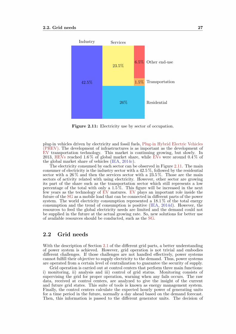
2.2. Grid needs 27
42.5%
Industry
26% Residential
23.5%
Services
1.5% Transportation
6.5% Other end-use
Figure 2.11: Electricity use by sector of occupation.
plug-in vehicles driven by electricity and fossil fuels, Plug-in Hybrid Electric Vehicles(PHEV). The development of infrastructures is as important as the development ofEV transportation technology. This market is continuing growing, but slowly. In2013, HEVs reached 1.6% of global market share, while EVs were around 0.4% ofthe global market share of vehicles (IEA, 2014c).
The electricity consumed by each sector can be observed in Figure 2.11. The mainconsumer of electricity is the industry sector with a 42.5%, followed by the residentialsector with a 26% and then the services sector with a 23.5%. Those are the mainsectors of activity related with using electricity. However, other sector are growingits part of the share such as the transportation sector which still represents a lowpercentage of the total with only a 1.5%. This figure will be increased in the nextfew years as the technology of EV matures. EV plays an important role inside thefuture of the SG as a mobile load that can be connected in different parts of the powersystem. The world electricity consumption represented a 18.1% of the total energyconsumption and the trend of consumption is positive (IEA, 2014d). However, theresources to feed the global electricity needs are limited and the demand could notbe supplied in the future at the actual growing rate. So, new solutions for better useof available resources should be conducted, such as the SG.
2.2 Grid needs
With the description of Section 2.1 of the different grid parts, a better understandingof power system is achieved. However, grid operation is not trivial and embodiesdifferent challenges. If those challenges are not handled effectively, power systemscannot fulfill their objective to supply electricity to the demand. Thus, power systemsare operated from a certain level of centralization to guarantee the security of supply.
Grid operation is carried out at control centers that perform three main functions:i) monitoring, ii) analysis and iii) control of grid status. Monitoring consists ofsupervising the grid for proper operation, warning when any fails occurs. The rawdata, received at control centers, are analyzed to give the insight of the currentand future grid states. This suite of tools is known as energy management system.Finally, the control centers calculate the expected hourly power of generating unitsfor a time period in the future, normally a day ahead based on the demand forecast.Then, this information is passed to the different generator units. The decision of
28 2. Grid Framework
which units should be generating for the next day is known as unit commitment andthe specification of the output power of each generator is the economic dispatch.Depending on the area, the unit commitment and economic dispatch values arecalculated based on external factors such as fuel costs or wholesale markets. Theseestimations from control centers are continuously updated to minimize the total costsgiven the load level, generator availability and transmission constraints. Controlcenters also manage to match small changes in load by adjusting generator unitsand meet the scheduled power exchanges with neighboring systems. This controlmechanism is called automatic generation control (MIT, 2011).
Grid operation is a complex process in which several factors have to be takeninto account. It faces countless problems which have to be solved in the lesstime possible to ensure that generation meets demand. However, electric powerindustry stakeholders (utilities, vendors, manufacturers, regulators, consumers andtheir advocates, and governments) have identified some issues that motivate a deepchange inside the grid. These changes are encouraged by different factors such asnew emergence technologies that help to increase the grid efficiency. The currentelectrical grid was designed to operate as a vertical structure consisting of generation,transmission, and distribution and supported with controls and devices to maintainreliability, stability, and efficiency (Momoh, 2012). This structure has barely changedsince its inception, although new advances have been incorporated to help theiroperation and management. These changes are not enough to face the currentneeds of the different electric power industry stakeholders. Some identified issuesmust be solved in order to improve the current system and evolve to the next gridgeneration. The principal problems are described below (El-hawary, 2014; Momoh,2012; Ekanayake et al., 2012):
Ageing infrastructure. In a lot of countries around the world, grids were deployedmore than 50 years ago when they suffered a rapid expansion to cover theirwhole national territory. Part of the devices from transmission and distributionnetworks are old and need replacement. The costs to introduce new equipmentare too high and grid operators cannot afford the investment necessary to replacethe old ones. However, the replacement is needed and it is a good opportunityto improve grid design and infrastructure according to current energy needs.
Electricity growth. Electricity is the final energy form more used at thepresent. Almost all devices used daily are powered by it, such as smartphones, computers, appliances, lights, etc. Demand will continue growing dueto different factors, such as the development of countries, coverage of newnecessities, etc. Electrical dependency is notable in developed countries andis growing in developing countries. Electricity is set to remain as the fastest-growing final form of energy worldwide. World electricity demand is expectedto grow by 2.1% per year on average over 2012-2040 with its share from therise in total energy use for all sectors and regions (IEA, 2014d). Figure 2.12(a)shows the electricity demand by regions in 2012 which is smaller for developedcountries and higher for developing and underdeveloped regions. The growth ofelectricity demand is exponential, as it can be observed in Figure 2.12(a). Chinaand India will consume more than twice the current electricity demand by 2040.In contrast, the OECD countries have a lower growth due to energy savingpolicies and the saturation of their electrical systems. Thus, it is necessarythat the grids are prepared to absorb this growth and supply the new demand.However, for the current structure of the grids, it is difficult to meet this newdemand. The reason is that the grids are operating at their capacity limitand the introduction of new demand will make the security of supply difficult.It is a great opportunity to invest and expand the network in both size andfunctionality.
Efficiency. The grid is a huge extensive network which presents losses in allits constituent parts despite ensuring electricity supply. However, its efficiencyis growing as a result of countless routine actions, although it is not enoughto tackle all the losses involved in the entire process. The largest losses inside
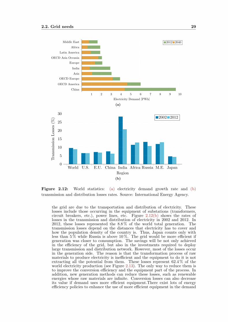
2.2. Grid needs 29
1 2 3 4 5 6 7 8 9 10
Middle East
Africa
Latin America
OECD Asia Oceania
Europe
India
Asia
OECD Europe
OECD America
China
Electricity Demand [PWh]
2012 2040
(a)
World U.S. E.U. China India Africa Russia M.E. Japan0
5
10
15
20
25
30
Region
Transm
ission
Losses(%
) 2002 2012
(b)
Figure 2.12: World statistics: (a) electricity demand growth rate and (b)
transmission and distribution losses rates. Source: International Energy Agency.
the grid are due to the transportation and distribution of electricity. Theselosses include those occurring in the equipment of substations (transformers,circuit breakers, etc.), power lines, etc. Figure 2.12(b) shows the rates oflosses in the transmission and distribution of electricity in 2002 and 2012. In2012, these losses represented the 8.8% of the world total generation. Thetransmission losses depend on the distances that electricity has to cover andhow the population density of the country is. Thus, Japan counts only withless than 5% while Russia is above 10%. The grid would be more efficient ifgeneration was closer to consumption. The savings will be not only achievedin the efficiency of the grid, but also in the investments required to deploylarge transmission and distribution network. However, most of the losses occurin the generation side. The reason is that the transformation process of rawmaterials to produce electricity is inefficient and the equipment to do it is notextracting all the potential from them. These losses represent 62.4% of theworld electricity production (see Figure 2.13). The only way to reduce them isto improve the conversion efficiency and the equipment part of the process. Inaddition, new generation methods can reduce these losses, such as renewableenergies whose raw materials are infinite. Conversion losses can also decreaseits value if demand uses more efficient equipment.There exist lots of energyefficiency policies to enhance the use of more efficient equipment in the demand
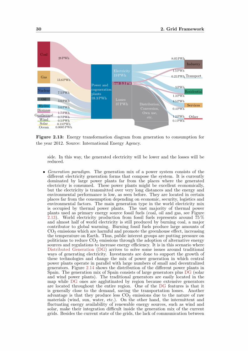
30 2. Grid Framework
Coal
Gas
Nuclear
Oil
Hydro
Biomass
Geothermal
WindSolarOcean
28PWh
13.6PWh
7.5PWh
3.6PWh
3.6PWh
1.7PWh
0.7PWh
0.5PWh0.13PWh0.0005PWh
Power and
cogeneration
plants
59.3PWh
Electricity
19PWh
Losses
37PWh Distribution,
Conversion,
Own use,
etc.
8.05PWh
0.25PWh
5PWh
4.5PWh
1.5PWh
1.3PWh
0.4PWh
1.2PWh
0.1PWh
Heat 3.3PWh
Industry
Transport
Residential
Services
Other
Figure 2.13: Energy transformation diagram from generation to consumption for
the year 2012. Source: International Energy Agency.
side. In this way, the generated electricity will be lower and the losses will bereduced.
Generation paradigm. The generation mix of a power system consists of thedifferent electricity generation forms that compose the system. It is currentlydominated by large power plants far from the places where the generatedelectricity is consumed. These power plants might be excellent economically,but the electricity is transmitted over very long distances and the energy andenvironmental performance is low, as seen before. They are located in certainplaces far from the consumption depending on economic, security, logistics andenvironmental factors. The main generation type in the world electricity mixis occupied by thermal power plants. The vast majority of thermal powerplants used as primary energy source fossil fuels (coal, oil and gas, see Figure2.13). World electricity production from fossil fuels represents around 75%and almost half of world electricity is still produced by burning coal, a majorcontributor to global warming. Burning fossil fuels produce large amounts ofCO2 emissions which are harmful and promote the greenhouse effect, increasingthe temperature on Earth. Thus, public interest groups are putting pressure onpoliticians to reduce CO2 emissions through the adoption of alternative energysources and regulations to increase energy efficiency. It is in this scenario whereDistributed Generation (DG) arrives to solve some issues around traditionalways of generating electricity. Investments are done to support the growth ofthese technologies and change the mix of power generation in which centralpower plants operate in parallel with large numbers of small and decentralizedgenerators. Figure 2.14 shows the distribution of the different power plants inSpain. The generation mix of Spain consists of large generators plus DG (solarand wind power plants). The traditional generators are easily located in themap while DG ones are agglutinated by region because extensive generatorsare located throughout the entire region. One of the DG features is that itis generally close to the demand, saving the transportation losses. Anotheradvantage is that they produce less CO2 emissions due to the nature of rawmaterials (wind, sun, water, etc.). On the other hand, the intermittent andfluctuating energy availability of renewable energy sources, such as wind andsolar, make their integration difficult inside the generation mix of the currentgrids. Besides the current state of the grids, the lack of communication between
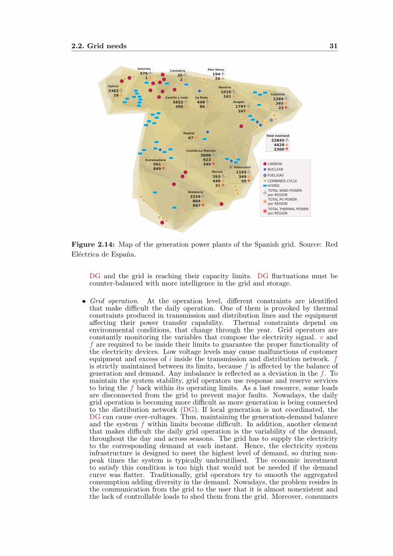
2.2. Grid needs 31
Murcia
26344031
Andalucía
3324869997
C. Valenciana
119334950
Castilla-La Mancha
3800923349
Total mainland
2284544282300
Aragón
1797167
Navarra
1016161
País Vasco
19426
La Rioja
44886
Castilla y León
5652495
Cantabria
352
Asturias
4761
Galicia
336216
TOTAL PV POWER
per REGION
CARBON
NUCLEAR
FUEL/GAS
COMBINED CYCLE
TOTAL THERMAL POWER
per REGION
HYDRO
TOTAL WIND POWER
per REGION
Extremadura
561849
Madrid
67
Cataluña
128426523
Figure 2.14: Map of the generation power plants of the Spanish grid. Source: Red
Electrica de Espana.
DG and the grid is reaching their capacity limits. DG fluctuations must becounter-balanced with more intelligence in the grid and storage.
Grid operation. At the operation level, different constraints are identifiedthat make difficult the daily operation. One of them is provoked by thermalconstraints produced in transmission and distribution lines and the equipmentaffecting their power transfer capability. Thermal constraints depend onenvironmental conditions, that change through the year. Grid operators areconstantly monitoring the variables that compose the electricity signal. v andf are required to be inside their limits to guarantee the proper functionality ofthe electricity devices. Low voltage levels may cause malfunctions of customerequipment and excess of i inside the transmission and distribution network. fis strictly maintained between its limits, because f is affected by the balance ofgeneration and demand. Any imbalance is reflected as a deviation in the f . Tomaintain the system stability, grid operators use response and reserve servicesto bring the f back within its operating limits. As a last resource, some loadsare disconnected from the grid to prevent major faults. Nowadays, the dailygrid operation is becoming more difficult as more generation is being connectedto the distribution network (DG). If local generation is not coordinated, theDG can cause over-voltages. Thus, maintaining the generation-demand balanceand the system f within limits become difficult. In addition, another elementthat makes difficult the daily grid operation is the variability of the demand,throughout the day and across seasons. The grid has to supply the electricityto the corresponding demand at each instant. Hence, the electricity systeminfrastructure is designed to meet the highest level of demand, so during non-peak times the system is typically underutilised. The economic investmentto satisfy this condition is too high that would not be needed if the demandcurve was flatter. Traditionally, grid operators try to smooth the aggregatedconsumption adding diversity in the demand. Nowadays, the problem resides inthe communication from the grid to the user that it is almost nonexistent andthe lack of controllable loads to shed them from the grid. Moreover, consumers
32 2. Grid Framework
are requiring more transparency in the consumption and new pricing modelsto grid operators. This lack of information in the distribution side is not onlyaffecting consumers, but also to the appearance of new products, services andmarkets and the accommodation of all DG and storage options, such as theEV. It is thought that in future the electrification of domestic heating loadsand the EV charge will lead to a greater capacity of flexible loads. This wouldhelp to maintain the network stability, reduce the requirements for reserve powerfrom part-loaded generators and the need for network reinforcement. Therefore,utilities need to adopt information and communication technologies to handlenew operational scenarios and challenges while maintaining profitability andinvesting in infrastructure.
Reliability and sustainability. Electricity security is a matter of keepingelectricity available to all connected users, within acceptable standards andthe amounts desired at any given time. At present, consumers require anincreasingly reliable electricity supply as more and more critical loads areconnected. The traditional approach to improve reliability was based onthe installation of additional redundant circuits, at considerable capital costand environmental impact. Other measures consist of disconnecting thefaulty circuit, so no action was required to maintain supply after a fault.However, recent system failures and blackouts have focused attention on tryingto increase system reliability. Reliability could be defined in terms of twobasic and functional aspects: adequacy and security. The system adequacyis the capability of the power system to meet changes in aggregating powerrequirements, using existing and new resources. On the other hand, the systemsecurity consists of maintaining the supply even with unexpected surges orsudden disruptions in demand. Accomplishing both features require efficiency,time and investment. In spite of the system fast response to changes indemand, it is not enough when the variability is too high. That is one reasonto interconnect the power systems of different regions, in order to guaranteethe supply. In addition, when a fault occurred and a blackout is produced,the reactions of grid operators are fast but not enough. The demand growthmakes necessary to increase the response to changes in the demand as wellas the need for more generation to cover this increase. However, the currentflexibility of the power systems is not optimized since its capability to alterthe consumption or generation in a rapid and large imbalance is relativelylow. For a greater adequacy, numerous mechanisms can be introduced, suchas the electricity trading, storage systems or more automation in the demand.About the security of the power systems, the ability of the grid for self-healing(anticipating responses to system disturbances) is very low. They only respondto prevent further damage and are focused on protecting assets following afault. Efficient and reliable electricity transport are fundamental to maintainfunctioning economies and societies. By watching these system features andincreasing their efficiency, grid sustainability could also be incremented as CO2emissions decrease and more renewable energies are integrated.
Investment and costs. The global generation costs are rising their figuresas demand is also growing. Generation investments are required to meetthe demand. Traditionally the investments were done in large power plantswhich can generate large amounts of electricity. However, nowadays theseinvestments are being transferred to smaller generators that are closer to theconsumption and use renewable energy. Different reasons support these changeof investments. One of them is the raising prices of raw primary materials,especially fossil fuels because reserves are dwindling. But also regulatorypressures are changing the model of investment, such as regulations in favorof the CO2 emission reductions or the improvement of electricity savings.Special efforts are being done by investors to afford new models to optimizeassets and operate efficiently. The investments are recovered through regulatedor competitive wholesale electricity prices and, to a lesser extent, supportivemeasurements from the governments. New markets are being developed, such

2.3. Grids evolution: towards the Smart Grid 33
as electrification of transport, to favor a major energy trading and expand theuse of electricity. This results in a power system more complex to operateand the necessity to adequate it to these new products and services. Thus, highinvestments have been done in the infrastructure (transmission and distributionnetworks) to expand the grid, meeting higher demand and stability. Success infinancing all the needed investments depends largely on governmental policiesand regulatory frameworks. But governments should reduce the political andregulatory uncertainties in order to generate a market attractive for investors.Combined with the increasing demand, higher prices are set to drive upelectricity bills. The price that a consumer pays for electricity has severalcomponents, some of them are: wholesale price to cover generation cost plusa margin, cost of transmitting and distributing the electricity, retail costs andtaxes.There are high differences in electricity prices depending on the region.Therefore, regulators are pushing for more competitive and lower energy prices.Also, improvements in energy efficiency could substantially moderate the impactof rising prices on electricity bills.
It is necessary that the grid improves its behavior to continue supplying electricityto consumers in terms of quality and security. In addition, if those needs arenot tackled in the near future, the power system will continue ageing withoutbeing able to incorporate new opportunities as they arise into the market scene.Improving the reliability, availability, and efficiency of the grid would benefit allmembers of the grid, reduce the costs and investments in the system and givethe grid more responsiveness and flexibility. Apart from the economic and policymotivations, a proper grid development would also contribute to the advance inemerging technologies, such as communications, computing power, energy storage,and renewable generation. These new advances would facilitate new services andimprove monitoring, control, communication and self-healing technologies. Moreover,making consumers participant in the grid structure will optimize the operation of thesystem and provide them with information and choice of supply. The promise of asmarter grid is done in which all the actual concerns are solved and the quality of thesystem is improved to advance towards the future.
2.3 Grids evolution: towards the Smart Grid
As explained in Section 2.2, the grid has recently faced important challenges to secureelectricity supply in a more efficient way according to more restrictive regulations.The advance of new technologies has helped to alleviate some problems in the past.However, there is a pressing need to accelerate the grid development that addressesthe global challenges of energy security, climate change and economic growth withadvanced low-carbon energy technologies. It is in this scenario where a new conceptof grid arises known as Smart Grid (SG). The SG also receives different names, smartelectrical/power grid, intelligent grid, intelligrid, futuregrid, intergrid, or intragrid,but they all consist of enhancing the 20th century power system (Fang et al., 2012).The “smartening” of the grid is an evolutionary process that involves adding newelements at the same time that the communication infrastructure is improved tomanage each part of the grid. This evolution is shown in Figure 2.15, in whichdifferences between the past, present and expected future of the grid are appreciated.It is fundamental not only a higher integration of every system part, but also tofacilitate the entry of new agents and technologies inside the grid. As shown in Figure2.15, over the years the grid has been responsible for expanding the communicationnetwork between its parts. However, it remains to cover the last few kilometers relatedto the users. Although many regions have already begun to “smarten” their electricitysystems, all regions will require significant additional investment and planning toachieve a smarter grid (IEA, 2011).
There is not a specific definition of what a SG must be. The reason for notadopting only one concept is due to the diversity of power systems around the world,in spite of sharing some features in common. There are differences mainly due to the
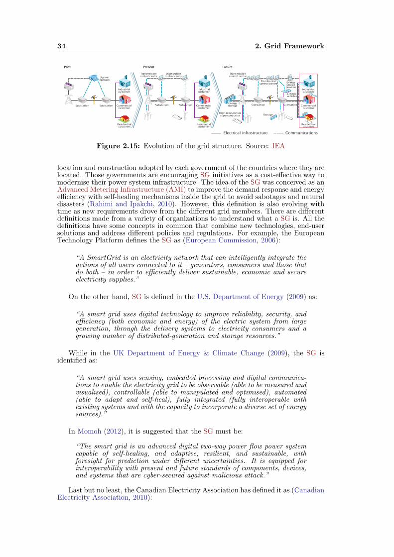
34 2. Grid Framework
Figure 2.15: Evolution of the grid structure. Source: IEA
location and construction adopted by each government of the countries where they arelocated. Those governments are encouraging SG initiatives as a cost-effective way tomodernise their power system infrastructure. The idea of the SG was conceived as anAdvanced Metering Infrastructure (AMI) to improve the demand response and energyefficiency with self-healing mechanisms inside the grid to avoid sabotages and naturaldisasters (Rahimi and Ipakchi, 2010). However, this definition is also evolving withtime as new requirements drove from the different grid members. There are differentdefinitions made from a variety of organizations to understand what a SG is. All thedefinitions have some concepts in common that combine new technologies, end-usersolutions and address different policies and regulations. For example, the EuropeanTechnology Platform defines the SG as (European Commission, 2006):
“A SmartGrid is an electricity network that can intelligently integrate theactions of all users connected to it – generators, consumers and those thatdo both – in order to efficiently deliver sustainable, economic and secureelectricity supplies.”
On the other hand, SG is defined in the U.S. Department of Energy (2009) as:
“A smart grid uses digital technology to improve reliability, security, andefficiency (both economic and energy) of the electric system from largegeneration, through the delivery systems to electricity consumers and agrowing number of distributed-generation and storage resources.”
While in the UK Department of Energy & Climate Change (2009), the SG isidentified as:
“A smart grid uses sensing, embedded processing and digital communica-tions to enable the electricity grid to be observable (able to be measured andvisualised), controllable (able to manipulated and optimised), automated(able to adapt and self-heal), fully integrated (fully interoperable withexisting systems and with the capacity to incorporate a diverse set of energysources).”
In Momoh (2012), it is suggested that the SG must be:
“The smart grid is an advanced digital two-way power flow power systemcapable of self-healing, and adaptive, resilient, and sustainable, withforesight for prediction under different uncertainties. It is equipped forinteroperability with present and future standards of components, devices,and systems that are cyber-secured against malicious attack.”
Last but no least, the Canadian Electricity Association has defined it as (CanadianElectricity Association, 2010):

2.3. Grids evolution: towards the Smart Grid 35
“The smart grid is a suite of information-based applications made possibleby increased automation of the electricity grid, as well as the underlyingautomation itself; this suite of technologies integrates the behaviour and ac-tions of all connected supplies and loads through dispersed communicationcapabilities to deliver sustainable, economic and secure power supplies.”
There are other definitions besides those already mentioned here. They presentthe SG as an opportunity to evolve the actual status of the grid and improve itsoperation. Some people believe that SGs are nothing more than a step forward tomodernize a “dumb network”. However, this assessment is totally wrong because the“smartening” of the grid consists of interconnecting all the parts to have control ofeach one in real time for better utilization of resources. In this Thesis, a broaderview of the term and what the SG involves are addressed because the term SG meansdifferent things to different people and its meanings are continuously evolving.
So far, the global vision of the SG gathers together the different parts of the currentgrid and adds different communication technologies with computational capabilitiesto provide favorable attributes that enhance its operation (Gharavi and Ghafurian,2011). A grid to become smart must include the following attributes among others(Fang et al., 2012; El-hawary, 2014; IEA, 2011):
Optimised and efficient. The SG incorporates the latest technologies to optimisethe use of its assets, in order to meet the increasing demand without addingextra infrastructure. Dynamic ratings are used to optimise the capacity ofthe system, allowing greater demand by continuously monitoring and ratingtheir capacities. Real-time monitoring and system control allow increasing theequipment efficiency through condition-based maintenance, signalling the rightinstant in which equipment maintenance is needed. Moreover, this platform willallow a smarter operation of the delivery system, rerouting power and workingautonomously, pursuing efficient asset management. Monitoring and controllingthe assets of the power systems allow reducing losses and eliminate congestion,including utilising them depending on what is needed and when it is needed toincrease the efficiency of the system. In addition, operating efficiency increaseswhen selecting the least-cost energy-delivery system available through thesetypes of system-control devices. Giving real-time consumption measures to userswill provide them with the information needed to modify their consumptionprofile based on individual preferences (pricing, efficiency, etc.) to enhance theoperation of the power system.
Integration. One of the virtues of the SG is the capability to integrate insidethe power system any generation technology without wasting electricity. Itaccommodates not only large centralised power plants, but also the growingarray of customer-sited distributed energy resources. This integration coversdifferent technologies including renewable, small-scale combined heat and power,and energy storage, which will increase rapidly all along the value chain, fromsuppliers to marketers to customers. Thus, the SG will provide simplifiedinterconnection similar to “plug-and-play”.
Participation. Enabling two way communication through different parts ofthe power system would help to decrease the peak-valley difference in thedaily demand. The reason is that consumers help to balance supply anddemand, ensuring reliability by modifying the way they use and purchaseelectricity. These modifications come as a result of consumers having choicesthat motivate different purchasing patterns and behaviors. These choices involvenew technologies, new information about their electricity use, and new forms ofelectricity pricing and incentives.
New horizons. The SG creates new opportunities and markets for itsdifferent participants. The efficient operation of the markets gives users theopportunity to choose among competing services. SG opens access to marketsthrough increased transmission paths, aggregated supply and demand response

36 2. Grid Framework
initiatives, and ancillary service provisions, which are those services thatfacilitate and support the continuous flow of electricity. In order to achievethe incorporation of these new markets, power system operators must managesome different variables such as energy, capacity, location, time, rate of changeand quality. Regulators, owners/operators and consumers need the flexibilityto modify the business rules in order to suit operating and market conditions.
Power quality. The SG is able to supply varying power grades and prices to allthe different consumers that are inside the power system. It is able to supplythe power quality necessary that meets the different needs of consumers, free ofsags, spikes, disturbances and interruptions to power the different loads of thedigital economy. Not all commercial enterprises, and certainly not all residentialcustomers, need the same quality of power. The cost of premium power-qualityfeatures can be included in the electrical service contract. Advanced controlmethods monitor essential components, enabling rapid diagnosis and solutionsto events that impact power quality, such as lightning, switching surges, linefaults and harmonic sources.
Resilient. The SG assures and improves the reliability and security of supply asit becomes more decentralized and reinforced with security protocols. Resilienceof the SG refers to the ability of a system to react to unexpected events(disturbances, attacks, natural disasters, etc.) by isolating problematic elementswhile the rest of the system is restored to normal operation. Some protectivemeasures are predictive maintenance, self-healing and strengthening the securityof supply through enhanced transfer capabilities. These self-healing actionsresult in reduced service interruptions to consumers and help service providersto better manage the delivery infrastructure.
Sustainable. The advance of global climate change is slowed down thanks toa high integration of low carbon technologies inside the SG. The reduction offossil fuels, through new ways of generation and the use of EV, is favoringa path towards significant environmental improvements. In addition, thereduction in demand variability will improve the operation of the systemand a better operation that affects positively the environment. Using localrenewable generators will decrease the environmental impact in reducing bothCO2 emissions and relevant visual effects of large power plants.
Thus, a possible definition of the SG that includes all these concepts is suggested:
A SG is an electricity network that uses communication technologies to co-ordinate the needs and capabilities of all generators, grid operators, end-users and electricity market stakeholders to operate all parts of the systemas efficiently as possible, minimising overall costs and environmentalimpacts while maximising system reliability, resilience and stability.
In spite of the benefits of the upgraded grid, there are also some impedimentsand drawbacks that make difficult its adoption. These concerns are related with thedifferent parts that shaped the SG and its deployment. Various barriers have beenidentified and are described below (El-hawary, 2014; Luthra et al., 2014):
Complexity. In the process of “smartening” the grid, it is necessary to deploysome technologies in order to assure the communication among all the gridmembers and to make the SG possible. However, in the process to increase thedegree of communication, the grid operation is complicated as more elements areincorporated in its infrastructure. The main reason of this grade of complexityis the huge amount of data that grid operators manage for a precise functioningof the system. In addition, the integration of new agents such as renewableenergies, distributed generation or storage systems, further complicates thepower system structure and requires their coordination and efficiently linkingwith the grid.
2.3. Grids evolution: towards the Smart Grid 37
Technology awareness. Additional infrastructure will be required for thedevelopment and operation of SG technologies. The automated control andsensing systems will require a modern communication infrastructure to performits daily operation. Other elements are also required such as sensors, intelligentelectronic devices, distributed energy resources, cyber security devices, advancedmetering systems and other end-use devices which need to be added in thepresent electricity system. Experts have identified the bi-directional flow ofcommunication as the back bone of the SG. However, there are some concernsabout adding all these elements. One of them is the additional costs thatsuppose providing to grid with these elements, since the industry wants to workwith traditional methods for safe and guaranteed return on investment. Industryis also worried with the concern that users do not require all the services that theSG technologies offer to them. So, the industry attitude towards the innovationis not enthusiastic and they have fear of adopting newer technologies. Anotherconcern is the maturity of the technologies to be deployed. New technologiesare still emerging and they are not yet validated which is slowing down thedevelopment of the SG. Another concern with SG technologies inside is thelack of clear standards to support system interoperability. Many proprietarystandards are in use today, which are making difficult the development of thesetechnologies. Thus, it is necessary to replace them with open standards toencourage, complete, stabilize and normalize them.
Economic. The deployment of the SG will require huge amounts of investmentsrelated to transfer the necessary technology, adequate the infrastructure andcommunication systems, hire skilled professionals, R&D work and integrationof new sources of generation. In spite of the SG benefits, investors are notinterested to invest in its deployment until universal standards are adoptedand the return on investments are guaranteed. In addition, there are notspecific policies and regulations for free markets tariffs and it is a strongpolitical commitment required and global cooperation to organize the dynamicsof energy market. Thus, private investment is discouraged frequently due tothe lack of revenue uncertainty and sufficient market base. One method toactivate the private investment is that governments provide some incentivesand subsidies to support the cost burden. This cost burden should be sharedamong investors, governments and/or potential beneficiaries to alleviate someof these difficulties. Nowadays many developed and developing nations affectedby the global recession are struggling to pay for renewal of their entire majorinfrastructure and are facing financial challenges.
Security. The deployment of ICTs introduces vulnerabilities to the system basedon potential cyber attacks. ICTs may be vulnerable to worms, viruses, denial-of-service attacks, malware, phishing and user errors that compromise integrity andavailability. Moreover, some aspects of the grid regulations may make difficultto ensure the cyber security of SG systems. Meanwhile, utilities are focusingon regulatory compliance instead of comprehensive security and consumers arenot being adequately informed about these risks. It is necessary the adoptionof models that work to develop solutions for cyber security, while allowing theuse of the data collected. Analyzing and implementing SG security may be achallenging task, considering the scale of the potential damages that could becaused by cyber attacks.
Data privacy. The use of ICTs allows collecting and access data of differentkind, such as electricity consumption, usage, production, etc. There are someconcerns about the risks related to how that data is used, shared, stored andaccessed. These concerns need to be addressed appropriately to gain consumeracceptance and trust. Organizations must establish internal privacy policies andsupporting procedures to protect the data coming from the different parts andespecially the data from users. The privacy policies must assure some specialtopics, such as how the information should be retained, distributed internally,shared with third parties, secured against breach, etc. In addition, SG services
38 2. Grid Framework
and products should provide a privacy notification that describes how the datais collected and how that information will be processed. The data access has tobe restricted and controlled in order to ensure that only specific individuals cangain access to confidential information. Some technologies can also be usefulto enhance the data privacy such as encryption, steganography or aggregationmethodologies to remove personally identifiable information from collections ofenergy usage data.
Public awareness. At early stages of the SG implementation, the educationalaspects are vital to the adoption of the SG by the different actors. Generalpublic needs to be educated through proper managed awareness programsabout the benefits of SG and technicalities of its usage, in order to make themparticipant through the use of advanced metering and two-way communicationavailable. If this situation is not handled appropriately, it can be detrimentalto the development of a market which helps the return of investment of privateinitiatives. Nowadays, customers are not massively adopting new technologiesto manage their electricity consumption due to the lack of understanding andproper incentives. Thus, advocates need to be able to explain and clearlyidentify the benefits of each SG component to the customers that are thepotential key to service success.
Policies and regulatory framework. The traditional regulatory system needsto evolve and be modified, in order to encourage the utilities’ investmenttowards the SG. Current regulations were created long ago and they wereappropriate for those times, but now they are obsolete. Traditional regulatorysystems are not harmonized and tend to discourage investment in innovativetechnologies. The key for good policies and regulations is to find the rightbalance in sharing costs, benefits and risks. The responsibility for achievingthis balance lies with regulators and, in some cases, legislators, but must includeinput from all stakeholders. That is why a collaboration among stakeholdersis necessary to impulse the development of a regulatory framework appropriateto the development of the SG. Moreover, specific policies in the consumer sideare required to guarantee that they are protected and assure their benefits.The reason is that consumers are typically not provided with either the serviceoptions or pricing information needed to manage their consumption. Thus, it isrequired that the SG customer policies fall into consumer feedback, protectionand pricing.
These are the main barriers that are hindering the development of the SG. In orderto get the SG deployment and benefit from it, it is necessary to tackle all of them.Consumer awareness, creation of a regulatory framework and economic investmentsare the keys in the development of the SG, since technologies involved are matureenough. Demonstrators are being developed all around the world to prove the benefitsof the SG and validate its possible deployment at large scale, while searching for acost-effective way to make it feasible. Governments are accelerating the installationof SG pilots with some investment initiatives as an opportunity to renew their gridsand as an important commercial opportunity to offer new services. In order to havea better understanding of the current state of pilots around the world, some nationalinitiatives are described as follows:
China. The Chinese government stated in the 12th Five-Year Plan (2011–2015)that the SG development is a national priority for the energy sector (Xu et al.,2014). The drivers for the developing of the SG are the rapid economic growth,the uneven geographical distribution of electricity generation and consumptionand the impressive increase of total energy use, which is still dominated byfossil-fuel-based thermal power generation (Ekanayake et al., 2012). China’sState Grid Corporation outlined plans in 2010 for a pilot SG programme thatmaps out deployment to 2030. It has developed a long-term stimulus planinvestment in SG which will reach at least 96USD billion by 2020 (IEA, 2011).

2.3. Grids evolution: towards the Smart Grid 39
India. The Indian government is driving some SG initiatives as part of anemerging energy policy of central and state governmental entities. These initia-tives include the increased grid capacity to meet the growing electricity demand,rural electrification, and optimizing electrical usage through load managementand improving operational efficiencies. The Indian SG is emphasizing the needof private investment in energy production/supply and unbundling the powersector from total government control as well as a new regulatory framework todevelop all the agents involved in the SG. The priorities to modernize the Indiangrid consist of reducing aggregate technical and commercial losses, automationto monitor and control the flow of power to/from the loads on an almostreal-time basis, improvement of system reliability, and intelligently managedloads, congestion, and power shortfall. The Smart grid Forum contributesto the Indian SG vision on advisory basis, coordinating with the Smart GridTask Force. The work groups, in which the two organizations are divided,are: advanced transmission, advanced distribution, communications, metering,consumption and load control, policy and regulation, and architecture anddesign (Samantaray, 2014).
USA. In the USA, the initiatives of the SG began with a public law publishedon December 2007 (United States, 2007). In this law, the government supportsthe modernisation of the electricity transmission and distribution networks tomaintain a reliable and secure electricity infrastructure. The USA government iscurrently emphasizing the need of performing studies to identify characteristicsof the current grid, identifying key technologies that are needed, and proposinga plan for technology deployment in both the short and long term, consideringtechnological, societal, economical, and legislative aspects. The investmentplanned by the government consists of 4.5USD billion to grid modernisation,3.48USD billion for quick integration of proven technologies into existing electricgrids, 435USD million for regional SG demonstrations and 185USD million forenergy storage and demonstrations (IEA, 2011).
European Union (EU). Meanwhile, the EU through the SmartGrids TechnologyPlatform published its vision of the SG strategy for Europe’s electricity networksin 2006 (European Commission, 2006). The vision of the European SG consistsof integrating all low carbon generation technologies to encourage demand sideto play an active part in the supply chain. The key challenges identifiedby the SmartGrids Technology Platform that impact on the delivery of theEU-mandated targets for the utilisation of renewable energy, efficiency andcarbon reductions by 2020 and 2050, are: strengthening the grid, decentralisedarchitectures for system control, delivering communications infrastructure, en-abling an active demand side management, integrating intermittent generation,enabling DG and storage systems, and preparing for the EV (Ekanayake et al.,2012). Thus, the different countries inside the EU are developing differentparts of the SmartGrids Technology Platform key challenges. For example,in Germany, the E-Energy funding programme has several projects focusingon ICTs for the energy system. In France, the distribution operator ERDFis deploying 300000 smart meters in a pilot project based on an advancedcommunication protocol named Linky. In Spain, the government mandateddistribution companies to replace existing meters with new smart meters in2008; this must be done at no additional cost to the customers. The replacementof these smart meters has to be done before 2018 for all the Spanish territory.In Italy, the Ministry of Economic Development has also granted over 200EURmillion for SG demonstrators and network modernisation in Southern Italianregions. And also the success of the Telegestore project has awarded eighttariff-based funded projects on active medium voltage distribution systems, toprove advanced network management and automation solutions necessary tointegrate DG (IEA, 2011).
UK. The UK Department of Energy and Climate change in the UK Departmentof Energy & Climate Change (2009) identifies key aspects to the SG development
40 2. Grid Framework
in the UK. Rapid expansion of intermittent renewable and less flexible nucleargeneration in conjunction with the retirement of flexible coal generation,electrification of heating and transport, penetration of distributed energyresources which include DG, DSM and storage and increasing penetration ofEV (Ekanayake et al., 2012). In addition, the energy regulator OFGEM has aninitiative called the Registered Power Zone that will encourage distributors todevelop and implement innovative solutions to connect distributed generators tothe network. OFGEM has set up a Low Carbon Networks fund that will allowup to 500GBP millions support to projects that test new technology, operatingand commercial arrangements (IEA, 2011).
Japan. The Japanese government declared in 2009 that the CO2 emissions willbe reduced a 75% by 2020. In order to achieve this target, the Ministry ofEconomy, Trade and Industry set three committees to look into the SG. Thesecommittees centered their efforts in studying low-carbon power system, next-generation transmission and distribution networks and how can be deployedthe SG in the Japanese context (Ekanayake et al., 2012). The Federationof Electric Power Companies of Japan is developing a SG that incorporatessolar power generation by 2020 with government investment of over 100USDmillion (IEA, 2011). The project is called “The Field Test Project on OptimalControl Technologies for the Next-Generation Transmission and DistributionSystem” and was conducted by 26 electric utilities, manufacturing companiesand research laboratories in Japan in order to develop the technologies to solvethese problems. The Japanese government has announced a national smartmetering initiative and large utilities have announced SG programmes (IEA,2011).
Rest of the world. The Australian government announced the 100AUD million“Smart Grid, Smart City” initiative in 2009 to deliver a commercial-scale SGdemonstration project. Additional efforts in the area of renewable energydeployments are resulting in further study on SGs. In Brazil, a utilityassociation called APTEL has been working with the Brazilian government onnarrowband power line carrier trials with a social and educational focus. Someutility operators are developing some strategies to deploy the SG pilots: Amplais deploying smart meters, AES Eletropaulo has developed a smart grid businessplan using the existing fiber optic backbone and CEMIG has started a SGproject based on system architecture developed by the IntelliGrid Consortium.In South Korea, the government has invested in a pilot programme on JejuIsland of 65USD million, which consists of a fully integrated SG system for 6000households, wind farms and four distribution lines. South Korea has announcedplans to implement SG nationwide by 2030 (IEA, 2011).
To sum up, the SG is a new field of development for old power systems to evolvein a new stage where all the agents can be part of a beneficial environment. SG is stillat an early stage to be deployed and a lot of research has to be done before it arisesat its final stage. Although there is no clear definition of what should be a SG, thereare five key aspects in which all the different definitions converge, Figure 2.16 showsthem. The SG is based in the actual grid that integrates renewable energies, storagesystems and demand side management thanks to the information and communicationtechnologies. It is in the convergence of these five aspects that the innovation arisesand their confluence makes the members of the entire system to benefit from it,as well as the environment. However, it also faces a lot of barriers, although themost worrying problem is the lack of investment to carry out the development ofthese technologies. Currently, initiatives by organizations and government partiesare supporting young drivers and improvements in existing power grid as part of itsrenovation to approach to the SG.
For a better understanding, each key aspect of the SG is described. The gridwas actually defined in Section 2.1, the communication technologies are presented inSection 2.3.1, then in Section 2.3.2 the DG technologies are explained, after that theuse of storage systems is presented in Section 2.3.3 and finally in Section 2.3.4, theuser importance in the demand curve is described.
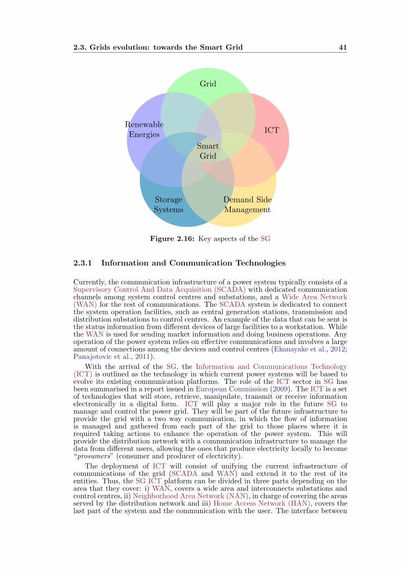
2.3. Grids evolution: towards the Smart Grid 41
Smart
Grid
ICT
Grid
Renewable
Energies
Storage
Systems
Demand Side
Management
Figure 2.16: Key aspects of the SG
2.3.1 Information and Communication Technologies
Currently, the communication infrastructure of a power system typically consists of aSupervisory Control And Data Acquisition (SCADA) with dedicated communicationchannels among system control centres and substations, and a Wide Area Network(WAN) for the rest of communications. The SCADA system is dedicated to connectthe system operation facilities, such as central generation stations, transmission anddistribution substations to control centres. An example of the data that can be sent isthe status information from different devices of large facilities to a workstation. Whilethe WAN is used for sending market information and doing business operations. Anyoperation of the power system relies on effective communications and involves a largeamount of connections among the devices and control centres (Ekanayake et al., 2012;Panajotovic et al., 2011).
With the arrival of the SG, the Information and Communications Technology(ICT) is outlined as the technology in which current power systems will be based toevolve its existing communication platforms. The role of the ICT sector in SG hasbeen summarised in a report issued in European Commission (2009). The ICT is a setof technologies that will store, retrieve, manipulate, transmit or receive informationelectronically in a digital form. ICT will play a major role in the future SG tomanage and control the power grid. They will be part of the future infrastructure toprovide the grid with a two way communication, in which the flow of informationis managed and gathered from each part of the grid to those places where it isrequired taking actions to enhance the operation of the power system. This willprovide the distribution network with a communication infrastructure to manage thedata from different users, allowing the ones that produce electricity locally to become“prosumers” (consumer and producer of electricity).
The deployment of ICT will consist of unifying the current infrastructure ofcommunications of the grid (SCADA and WAN) and extend it to the rest of itsentities. Thus, the SG ICT platform can be divided in three parts depending on thearea that they cover: i) WAN, covers a wide area and interconnects substations andcontrol centres, ii) Neighborhood Area Network (NAN), in charge of covering the areasserved by the distribution network and iii) Home Access Network (HAN), covers thelast part of the system and the communication with the user. The interface between
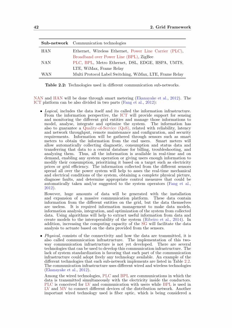
42 2. Grid Framework
Sub-network Communication technologies
HAN Ethernet, Wireless Ethernet, Power Line Carrier (PLC),
Broadband over Power Line (BPL), ZigBee
NAN PLC, BPL, Metro Ethernet, DSL, EDGE, HSPA, UMTS,
LTE, WiMax, Frame Relay
WAN Multi Protocol Label Switching, WiMax, LTE, Frame Relay
Table 2.2: Technologies used in different communication sub-networks.
NAN and HAN will be done through smart metering (Ekanayake et al., 2012). TheICT platform can be also divided in two parts (Fang et al., 2012):
Logical, includes the data itself and its called the information infrastructure.From the information perspective, the ICT will provide support for sensingand monitoring the different grid entities and manage those informations tomodel, analyse, integrate and optimize the system. The information hasalso to guarantee a Quality-of-Service (QoS), related with reliability, latencyand network throughput, remote maintenance and configuration, and securityrequirements. Information will be gathered through sensors such as smartmeters to obtain the information from the end users. Smart meters willallow automatically collecting diagnostic, consumption and status data andtransferring that data to a central database for billing, troubleshooting, andanalyzing them. Thus, all the information is available in real-time and ondemand, enabling any system operation or giving users enough information tomodify their consumption, prioritizing it based on a target such as electricityprices or grid efficiency. The information collected from the different sensorsspread all over the power system will help to asses the real-time mechanicaland electrical conditions of the system, obtaining a complete physical picture,diagnose faults, and determine appropriate control measures that could beautomatically taken and/or suggested to the system operators (Fang et al.,2012).
However, huge amounts of data will be generated with the installationand expansion of a massive communication platform. These data containinformation from the different entities on the grid, but the data themselvesare useless. It is required information management to make data models,information analysis, integration, and optimization of the system from collecteddata. Using algorithms will help to extract useful information from data andcreate models to the interoperability of the system (Ribeiro et al., 2014). Inaddition, increasing the computing capacity of the SG will facilitate the dataanalysis to actuate based on the data provided from the sensors.
Physical, consists of the connectivity and how the data are transmitted, it isalso called communication infrastructure. The implementation of this two-way communication infrastructure is not yet developed. There are severaltechnologies that can be used to develop this communication infrastructure. Thelack of system standardization is favoring that each part of the communicationinfrastructure could adopt freely any technology available. An example of thedifferent technologies that each sub-network implements are listed in Table 2.2.The communication infrastructure uses different wired and wireless technologies(Ekanayake et al., 2012).
Among the wired technologies, PLC and BPL are communications in which thedata is transmitted simultaneously with the electricity inside the conductors.PLC is conceived for LV and communication with users while BPL is used inLV and MV to connect different devices of the distribution network. Anotherimportant wired technology used is fiber optic, which is being considered a

2.3. Grids evolution: towards the Smart Grid 43
suitable option thanks to its deployment as communication network for theinternet. Among the wireless options are worthy to distinguish the standardsIEEE 802 series, which are a family of standards to support Local AreaNetworks (LAN) (Wireless LAN - IEEE 802.11, bluetooth - IEEE 802.15,WiMAX - IEEE 802.16). In addition, another communication network alreadydeployed that can be used by power systems is the cellular communicationsystems, consisting of different generations EDGE, HSPA, UMTS, LTE, etc.Other wireless communication technologies are the cognitive radios, microwavecommunications and satellite communications. There exist lots of standards oncommunications that could be part of the communication infrastructure of thefuture power system. This is causing serious concerns about the interoperabilityof this variety of systems inside the communication platform and how to assurethe integrity of the data (Fang et al., 2012).
Coming back to the architectural design of the communication system, it mustbe able to interconnect the different sub-networks: enterprise bus (connectscontrol centers, markets and generators), WAN (covers the transmissionnetwork), NAN (covers the distribution network) and HAN (covers the users).The communication channel, which is the path where data travels as a signal,has to connect the different entities of the communication system. Thecommunications normally are point-to-point but the channel between the sourceand destination could be dedicated or shared medium depending on the sub-network and the technology used. Communication channels are characterisedby their maximum data transfer speed, error rate, delay and communicationtechnology used. Thus, the communications infrastructure, used by powersystem, could consist of private utility communication networks (radio networks,meter mesh networks) or public carriers and networks (Internet, cellular, cableor telephone) (Panajotovic et al., 2011).
In conclusion, the ICTs are key to stablish the communication necessary to deploythe SG. It is required that the ICTs give coverage to all the members of the system,that is one of the reasons to use private and public communication channels. However,the security and privacy of the channel must be assured, ensuring the protection ofthe data and not suffering any cyber-attack to cause failures or users could be indanger. Not using a common set of standardized communication is making complexthe system structure, that is why the interoperability must be guaranteed insidethe ICT infrastructure. Finally, the ICT infrastructure needs to guarantee the QoSbecause of the existence of critical data (e.g. the grid status information) that mustbe delivered promptly.
2.3.2 Renewable Energies: the Distributed Generation paradigm
Once that the bidirectionally of the information is assured by ICT infrastructures,it is possible to take advantage of new generation technologies spread out all overthe grid. With this new communication system, a door is opened to integrate allthe generation technologies inside the SG. So far, only huge isolated power plantswere used as the main power source of electricity. However, with the rise of differentrenewable energy technologies in power systems, this paradigm is rapidly changingdue to the possibilities that they offer. Renewable energies are understood as the setof energies that come continuously from resources which are naturally replenished on ahuman timescale and are derived from the sun, directly (thermal, photo-chemical, andphoto-electric) or indirectly (wind, hydro and biomass), or from natural movementsand environmental mechanisms (geothermal heat and tidal). Renewable energies donot include energy resources derived from fossil and nuclear fuels (Ellabban et al.,2014).
According to the European Renewable Energy Council, the renewable energiesare theoretically able to provide about 3000 times the total current world energyconsumption (Zervos et al., 2010). Figure 2.17 shows how these flows of energy areshared by different possible sources. The solar resource represents more than 90%of the total. The use of renewable energies has been extended in the last decades to
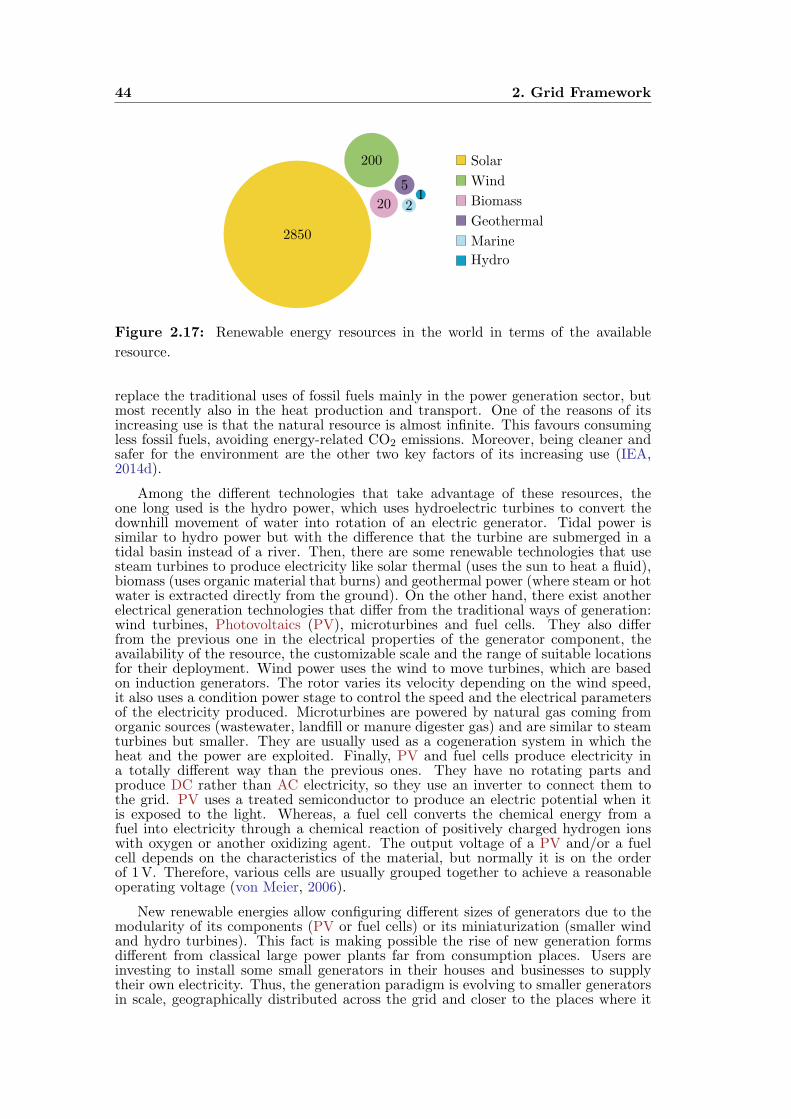
44 2. Grid Framework
2850
200
20
5
21
Solar
Wind
Biomass
Geothermal
Marine
Hydro
Figure 2.17: Renewable energy resources in the world in terms of the available
resource.
replace the traditional uses of fossil fuels mainly in the power generation sector, butmost recently also in the heat production and transport. One of the reasons of itsincreasing use is that the natural resource is almost infinite. This favours consumingless fossil fuels, avoiding energy-related CO2 emissions. Moreover, being cleaner andsafer for the environment are the other two key factors of its increasing use (IEA,2014d).
Among the different technologies that take advantage of these resources, theone long used is the hydro power, which uses hydroelectric turbines to convert thedownhill movement of water into rotation of an electric generator. Tidal power issimilar to hydro power but with the difference that the turbine are submerged in atidal basin instead of a river. Then, there are some renewable technologies that usesteam turbines to produce electricity like solar thermal (uses the sun to heat a fluid),biomass (uses organic material that burns) and geothermal power (where steam or hotwater is extracted directly from the ground). On the other hand, there exist anotherelectrical generation technologies that differ from the traditional ways of generation:wind turbines, Photovoltaics (PV), microturbines and fuel cells. They also differfrom the previous one in the electrical properties of the generator component, theavailability of the resource, the customizable scale and the range of suitable locationsfor their deployment. Wind power uses the wind to move turbines, which are basedon induction generators. The rotor varies its velocity depending on the wind speed,it also uses a condition power stage to control the speed and the electrical parametersof the electricity produced. Microturbines are powered by natural gas coming fromorganic sources (wastewater, landfill or manure digester gas) and are similar to steamturbines but smaller. They are usually used as a cogeneration system in which theheat and the power are exploited. Finally, PV and fuel cells produce electricity ina totally different way than the previous ones. They have no rotating parts andproduce DC rather than AC electricity, so they use an inverter to connect them tothe grid. PV uses a treated semiconductor to produce an electric potential when itis exposed to the light. Whereas, a fuel cell converts the chemical energy from afuel into electricity through a chemical reaction of positively charged hydrogen ionswith oxygen or another oxidizing agent. The output voltage of a PV and/or a fuelcell depends on the characteristics of the material, but normally it is on the orderof 1V. Therefore, various cells are usually grouped together to achieve a reasonableoperating voltage (von Meier, 2006).
New renewable energies allow configuring different sizes of generators due to themodularity of its components (PV or fuel cells) or its miniaturization (smaller windand hydro turbines). This fact is making possible the rise of new generation formsdifferent from classical large power plants far from consumption places. Users areinvesting to install some small generators in their houses and businesses to supplytheir own electricity. Thus, the generation paradigm is evolving to smaller generatorsin scale, geographically distributed across the grid and closer to the places where it
2.3. Grids evolution: towards the Smart Grid 45
is consumed (Pepermans et al., 2005). These new forms of generation are what isknown as Distributed Generation (DG).
The decentralization of the generation have great benefits for the grid. The systemsupport benefits are as follows (Pepermans et al., 2005; Barker and de Mello, 2000;von Meier, 2006):
0 7 14 21 24t(h)
Figure 2.18: Example of PV generation with aggregated consumption of a power
system. In blue the aggregated consumption of the power system, in yellow the DG
and in shadow grey the night hours are represented.
Loss reduction. By generating electricity closer to the places where it isconsumed, the electricity does not need to be transported large distances, sothe thermal losses of the power lines decrease.
Reliability and power quality. Generating electricity in more than one placeadds redundancy in the system that helps to enhance its security. For example,it helps to overcome easily sustained interruptions (voltage drops to zero) orsabotages along the power system. Related with power quality3, DG canincrease it by providing voltage support to rise the insufficient voltage of anarea or providing reactive power support to compensate it. So, if DG canprovide voltage support reliably, installation or upgrades of new hardware canbe avoided.
Avoiding upgrades in the transmission and distribution network. The installa-tion of DG reduces the constraints of the transmission and distribution networks,alleviating the power system size. The equipment inside the network has toaccommodate the peak load, but offsetting a demand amount with DG canprovide relief in the infrastructure (e.g. for a PV DG can be observed in Figure2.18). Thus, it is not necessary to invest in order to upgrade the infrastructurewhile maintaining reliability.
Grid support. DG could also contribute to provide auxiliary services to maintaina stable grid operation, such as generation on demand by operators, stabilisingthe frequency, etc.
3Power quality is referred to the waveform of i and v compared to an ideal sinusoidal one and the
balance between them.
46 2. Grid Framework
Economic savings. These new technologies offer some economic reductions. Theinvestment in grid infrastructure can be reduced, as well as reducing oversizingrelated to system demand or investment in new equipment to ensure systemreliability. Also, users can benefit from using DG locally by reducing thepurchase of external resources. In addition, DG can be used depending onthe electricity pricing, following an economic saving strategy. The costs are alsoshared by the different grid stakeholders, resulting in a collective benefit for allof them.
Environmental friendly. Apart from being increasingly cost-effective technolo-gies, they also have some environmental benefits. In general, DG consistsof renewable energies which are low emissions power supplies. Thus, thedependency from environmentally damaging fuels is reduced. Consequently, thelevels of greenhouse gas, toxic chemical emissions and other damaging emissionsare also reduced. For example, cogeneration technologies use waste materialsso the need of landfill sites are reduced.
On the other hand, DG faces important challenges for its fully adoption. The firstone is the high investment costs of some technologies. The problem is that for sometechnologies there are no economies of scale, which makes difficult their deployment.Moreover, there is not a clear financial credit to support the installation of DG in spiteof being considered as key technologies to decrease the harmful effects of electricitygeneration to the environment. Another issue is the need of extra protection andcoordination of the generation resources. The reason is that the flow of electricity isnow bidirectional, consequently the system is no longer a centralized, radial and flatsystem. At the distribution level there is not only consumption, but also generationis injected at this level. Thus, the equipments inside the distribution network canexperiment a flow of energy in the other direction for which they are not built. It isnecessary to introduce extra security elements such as switches or even change theequipment to support the bidirectionally flows of energy. The coordination issue isrelated with control and availability of resources. The problem of some renewableenergies is that they do not produce regularly the same amount of electricity anddepend on the weather and other variables which are difficult to predict. This factmakes difficult the generation scheduling and increases the operation complexity ofthe grid (Pepermans et al., 2005; von Meier, 2006). Finally, there are also someenvironmental concerns related to certain renewable energies. For example, someorganic fuels of biomass are crops destined to produce energy and some markets arechanging the way of cultivating some areas. Other concerns are related to the visualimpact of the technologies in the environment, such as large wind turbines or hugePV solar fields (Ellabban et al., 2014).
In spite of these deterrents, all these problems are minor drawbacks overcome bythe benefits that the DG possesses. The problem of the generation scheduling is notcrucial since it can be tackled in various ways, using predictive algorithms for propersystem integration or trying to design a system to meet the demand without anysurplus. About environmental, financial costs and protection issues, regulations andpolicies are the elements responsible for changing the actual situation and favor thedeployment of DG.
The election of a renewable technology in DG is decided based on how nearit is to the loads, however, it must also be environmentally compatible. Amongall the renewable energies available, the PV is the more suitable to almost anyapplication. PV is easy to deploy because it involves the least possible inconvenience:zero emissions, no noise, reduced aesthetic impact, different options can be used tointegrate it in buildings or other structures (for example, sunshade for windows orshading for parking lots), easy configuration of the generator adding or eliminatingPV panels and low maintenance of facilities (von Meier, 2006). Other technologiessuch as fuel cells require more supervision, or wind power requires better conditionsfor resource availability.
To sum up, the DG of renewable energy is presented as one of the alternativesto our present centralized and hierarchical power system. Many questions remainto be solved regarding their availability and their development to achieve greater
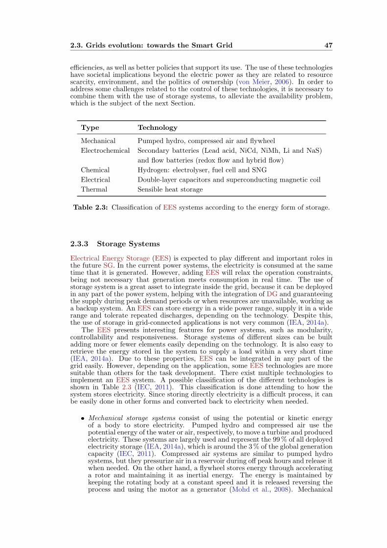
2.3. Grids evolution: towards the Smart Grid 47
efficiencies, as well as better policies that support its use. The use of these technologieshave societal implications beyond the electric power as they are related to resourcescarcity, environment, and the politics of ownership (von Meier, 2006). In order toaddress some challenges related to the control of these technologies, it is necessary tocombine them with the use of storage systems, to alleviate the availability problem,which is the subject of the next Section.
Type Technology
Mechanical Pumped hydro, compressed air and flywheel
Electrochemical Secondary batteries (Lead acid, NiCd, NiMh, Li and NaS)
and flow batteries (redox flow and hybrid flow)
Chemical Hydrogen: electrolyser, fuel cell and SNG
Electrical Double-layer capacitors and superconducting magnetic coil
Thermal Sensible heat storage
Table 2.3: Classification of EES systems according to the energy form of storage.
2.3.3 Storage Systems
Electrical Energy Storage (EES) is expected to play different and important roles inthe future SG. In the current power systems, the electricity is consumed at the sametime that it is generated. However, adding EES will relax the operation constraints,being not necessary that generation meets consumption in real time. The use ofstorage system is a great asset to integrate inside the grid, because it can be deployedin any part of the power system, helping with the integration of DG and guaranteeingthe supply during peak demand periods or when resources are unavailable, working asa backup system. An EES can store energy in a wide power range, supply it in a widerange and tolerate repeated discharges, depending on the technology. Despite this,the use of storage in grid-connected applications is not very common (IEA, 2014a).
The EES presents interesting features for power systems, such as modularity,controllability and responsiveness. Storage systems of different sizes can be builtadding more or fewer elements easily depending on the technology. It is also easy toretrieve the energy stored in the system to supply a load within a very short time(IEA, 2014a). Due to these properties, EES can be integrated in any part of thegrid easily. However, depending on the application, some EES technologies are moresuitable than others for the task development. There exist multiple technologies toimplement an EES system. A possible classification of the different technologies isshown in Table 2.3 (IEC, 2011). This classification is done attending to how thesystem stores electricity. Since storing directly electricity is a difficult process, it canbe easily done in other forms and converted back to electricity when needed.
Mechanical storage systems consist of using the potential or kinetic energyof a body to store electricity. Pumped hydro and compressed air use thepotential energy of the water or air, respectively, to move a turbine and producedelectricity. These systems are largely used and represent the 99% of all deployedelectricity storage (IEA, 2014a), which is around the 3% of the global generationcapacity (IEC, 2011). Compressed air systems are similar to pumped hydrosystems, but they pressurize air in a reservoir during off peak hours and release itwhen needed. On the other hand, a flywheel stores energy through acceleratinga rotor and maintaining it as inertial energy. The energy is maintained bykeeping the rotating body at a constant speed and it is released reversing theprocess and using the motor as a generator (Mohd et al., 2008). Mechanical
48 2. Grid Framework
storage systems can store electricity up to the order of MW, but they are largesystems and require considerable maintenance.
Electrochemical type of EES are also known as batteries and they are alongwith pumped hydro systems the oldest forms of EES. The electricity isstored chemically inside the battery. Secondary batteries consist of a liquid,paste, or solid electrolyte together with a positive electrode (anode) and anegative electrode (cathode) (Mohd et al., 2008). During the discharge process,electrochemical reactions occur in the two electrodes and a current is generatedbetween them. Reversing the process will charge the battery. There are differentchemicals used to build the battery: lead acid are the oldest and most widelyused, nickel cadium (NiCd) is also quite widespread, sodium sulphur (NaS) andlithium ion (Li-ion) (Chen et al., 2009). Li-ion are becoming an alternative tothe oldest batteries due to its efficiency (around the 100%), the increase lifecycle of the battery and its reduced shape for some applications (Chen et al.,2009). Flow batteries are also rechargeable batteries, but the energy is stored inone or more electroactive components, which are dissolved in liquid electrolytes.The electrolytes are stored in tanks and pumped through the electrochemical cellthat converts chemical energy directly to electricity and vice versa (IEC, 2011).There are two main types of flow batteries: redox and hybrid flow batteries.
Mechanical and electrochemical storage systems are the oldest types of EES andare already mature enough to be installed. However, new types of EES are indevelopment, such as the hydrogen systems. These storage systems consist of storingthe hydrogen generated in an electrolysis process. Once the hydrogen is produced,different alternatives are available for its use as an energy carrier: transport, heating,chemical industry, etc. The problem is that the efficiency is low (around 40%)compared to other technologies, but it can store large amounts of energy (IEC, 2011).Other EES systems are thermal ones, in which the electricity is used to heat or colda fluid and later used in different applications, such as space heating or cooling, hotwater production or electricity generation (Mohd et al., 2008). The last type of EESstores electricity directly: super capacitors and superconducting magnetic coils. Thefirst one has the features of batteries and capacitors and electricity is stored in theform of an electric field between two electrodes (Mohd et al., 2008). They are verydurable (8–10 years) with high efficiency (∼95%). However, they present a high self-discharge so energy has to be used quickly (Mohd et al., 2008). On the other hand,the superconducting magnetic energy storage consists of storing energy in a magneticfield created by the current flowing through a superconducting coil (IEC, 2011). Theypossess a fast response, but they require high operating costs, deep discharges andconstant activities (Mohd et al., 2008).
Some features to consider the election of a storage system are its maturity, lifecycle, costs, efficiency, environmental implications and density. Depending on thetechnology some of these features are better than others. For example, pumpedhydro, fuel batteries or fuel cells are suitable for energy management application,whereas flywheels, batteries and supercapacitors are more suitable for power qualityand Uninterruptible Power Supply (UPS) applications. EES provides the grid withsome advantages, such as (Mohd et al., 2008; IEC, 2011; Chen et al., 2009; Wadeet al., 2010):
Voltage control. Maintaining voltages within acceptable range implies that itprovides load factor correction, reduce the need to constrain generation, mitigateflicker, sags and swells, etc.
Frequency support. Reducing the imbalances between generation and consump-tion favors keeping the grid frequency within its limits for periods up to 30minutes.
Transient stability. Oscillations are reduced in the power signal by injecting orabsorbing real power.

2.3. Grids evolution: towards the Smart Grid 49
0 7 14 21 24t(h)
Figure 2.19: EV charging for load levelling during valley hours. In blue the
aggregated consumption of the power system, in red the valley filling technique using
the EV and in shadow grey the night hours are represented.
Power quality and reliability. Power quality is related with changes in magnitudeand shape of the voltage and current. Storage systems can help with harmonics,power factor, transients, flicker, etc, providing reliable electricity to consumers.EES could supply the consumption during interruption or blackouts, but alsoit could help to restore the network after faults.
Load levelling. A storage system is charged with excess power during low-demand periods and it is discharged when the power demand is on peak levels.
Spinning reserve. The power of an EES system is reserved to supply the loadimmediately when a fault occurs.
Power flow management. Redirecting power flows increases operation efficiencyand cost reductions in fuel. This property also contributes to the delay networkreinforcement, reduction of reverse power flows and minimization of losses.
In addition, EES could help in the energy market by arbitraging and balancingit. It could also help to reduce the variability of the DG, increase its yield from non-firm connections, compliance with energy security standards and support networkmanagement (assist islanded networks, support black starts, etc.) (Wade et al.,2010). The main reasons of storage absence in the grid are typically its costs andthe generation control possibilities of present power systems. It makes unprofitablethe deployment of new storage systems on a large scale. However, high investmentsin EES can be affordable when these costs are offset by higher revenues, such aspurchasing inexpensive electricity during low demand periods and later selling itto a higher price. Moreover, it could reduce financial losses associated with powerquality anomalies and outages, increase the revenue from renewable energy sources,reduce the variability of the generation, increase revenue for ancillary services, andavoid installing extra generation (Mohd et al., 2008). There are also some concernsabout the maturity of the technologies, its energy density, power capacity, life cycle,efficiency, discharge capability and environmental issues. Only two technologiesare currently mature enough, pumped hydro and lead-acid batteries, the rest arecurrently under development, although some technologies are almost mature such asLi-ion batteries (Chen et al., 2009). With respect to the efficiency, EES have highefficiencies depending on the technology, batteries, pumped hydro, compressed air andsupercapacitors present an efficiency above 60% (Chen et al., 2009). Although thedevelopment of EES is advancing, the life cycle and the discharging capacity are stillnot enough for its integration in some parts of the grid (IEA, 2014a). EES presentssome negative effects on the environment, fossil combustion, strong magnetic field,landscape damage and toxic remains (Chen et al., 2009). For example, the remains of
50 2. Grid Framework
the batteries are toxic and must be treated in order not to damage the environment.But it is still necessary a deeper analysis of the environmental implications of installingthe storage system, taking into account the installation and use of the system. Despiteall drawbacks found, EES is needed in the grid due to the flexibility that providesto the power systems. That is the reason why the storage level is expected to growto 10–15% from the current 3% in USA and European countries, and even higher inJapan in the near future (Chen et al., 2009).
Among EES systems, secondary batteries are gaining special importance becauseof two factors: integration with DG powered by renewable energies and the ElectricVehicle (EV). The use of batteries with DG will improve the usability of renewableenergy, since it will help to reduce the variability of the resource, charging the batterywith the electrical surplus and making it available when it is needed. On the otherhand, the EV market is growing and it is expected to continue this trend in the nextdecades (IEA, 2013). The reasons behind this growth are mainly due to lower batterycosts, reduction of CO2 emissions and reduction of the dependency from fossil fuels(IEC, 2011; IEA, 2013). The electrification of the transportation sector is associatedwith a massive deployment of EV in the coming years. This electrification supposesa paradigm shift in energy systems because the grid must be able to absorb a majorand new electric consumption. The penetration of the EV will have a great impact onthe distribution networks. And if it is not handled with care, it can lead to negativeeffects (II et al., 2011). The EV charge could become a serious problem due to theincrease of power from the distribution level and could affect transmission network oreven to the generation capacity of the grid causing an overall increase of the requiredinfrastructure. However, the EV charge offers a flexible load that the grid could useto enhance its functionality. Thus, these problems can be addressed from EV chargecoordination (Deilami et al., 2011; Mets et al., 2010). For example, in Figure 2.19,the charge of the EV is used to reduce the variability of the consumption, charging itat off-peak periods. Managing the charge of EV could support the grid and improveits operation through the reduction of power losses levelling the load (Deilami et al.,2011).
Finally, the integration of EES and in particular the EVs in the grid is increasinglyfeasible thanks to its participation in the SG. Due to the ICT platform, the chargeof the EV can be easily done by the grid. With Vehicle-to-Grid (V2G), EVs will benot only mere consumers but they will be used to provide power for specific electricmarkets. The EV charging management can be framed in the general concept of theDSM, which is discussed in Section 2.3.4.
2.3.4 Demand side management and electricity management strate-
gies
So far, new elements have been presented for their integration within power systemsto enhance them. However, the potential of these elements alone could benefit orharm the grid operation, depending on how they are managed. Thus, it is necessaryto provide grid operators with a number of tools to coordinate the new power flowsthat appear from the integration of DG renewable energies and EES together withICTs to reach them. It is in this framework in which users will play an importantrole in the SG, by helping to manage their demand towards energy efficiency.
Therefore, an increasing number of programs and policies are motivating usersto collaborate with the grid operators for its enhancement. All these programs areincluded within the concept of Demand Side Management (DSM). This concept isnot new, it appears in the 80s and was defined as “planning, implementation, andmonitoring of those utility activities designed to influence customer use of electricityin ways that will produce desired changes in the utility’s load shape, i.e., changes inthe time pattern and magnitude of a utility’s load” by Gellings (1985). Currently,DSM is defined as actions that influence the way that consumers use electricity inorder to achieve savings or higher efficiency in energy use. DSM is a global term thatincludes a variety of activities, such load management, energy efficiency, etc. in along-term perspective. Whereas the short-term perspectives are tackled by DemandResponse (DR) programs, which are actions that result in short-term reductions in
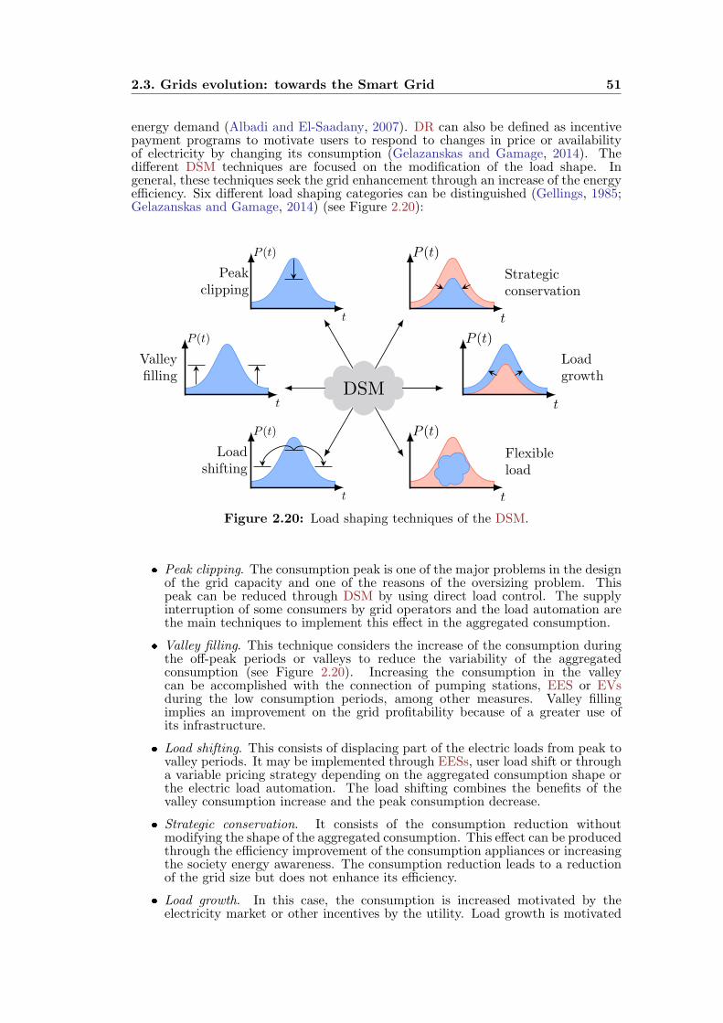
2.3. Grids evolution: towards the Smart Grid 51
energy demand (Albadi and El-Saadany, 2007). DR can also be defined as incentivepayment programs to motivate users to respond to changes in price or availabilityof electricity by changing its consumption (Gelazanskas and Gamage, 2014). Thedifferent DSM techniques are focused on the modification of the load shape. Ingeneral, these techniques seek the grid enhancement through an increase of the energyefficiency. Six different load shaping categories can be distinguished (Gellings, 1985;Gelazanskas and Gamage, 2014) (see Figure 2.20):
DSM
Peakclipping
t
P (t)
Valleyfilling
t
P (t)
Loadshifting
t
P (t)
Strategicconservation
t
P (t)
Loadgrowth
t
P (t)
Flexibleload
t
P (t)
Figure 2.20: Load shaping techniques of the DSM.
Peak clipping. The consumption peak is one of the major problems in the designof the grid capacity and one of the reasons of the oversizing problem. Thispeak can be reduced through DSM by using direct load control. The supplyinterruption of some consumers by grid operators and the load automation arethe main techniques to implement this effect in the aggregated consumption.
Valley filling. This technique considers the increase of the consumption duringthe off-peak periods or valleys to reduce the variability of the aggregatedconsumption (see Figure 2.20). Increasing the consumption in the valleycan be accomplished with the connection of pumping stations, EES or EVsduring the low consumption periods, among other measures. Valley fillingimplies an improvement on the grid profitability because of a greater use ofits infrastructure.
Load shifting. This consists of displacing part of the electric loads from peak tovalley periods. It may be implemented through EESs, user load shift or througha variable pricing strategy depending on the aggregated consumption shape orthe electric load automation. The load shifting combines the benefits of thevalley consumption increase and the peak consumption decrease.
Strategic conservation. It consists of the consumption reduction withoutmodifying the shape of the aggregated consumption. This effect can be producedthrough the efficiency improvement of the consumption appliances or increasingthe society energy awareness. The consumption reduction leads to a reductionof the grid size but does not enhance its efficiency.
Load growth. In this case, the consumption is increased motivated by theelectricity market or other incentives by the utility. Load growth is motivated
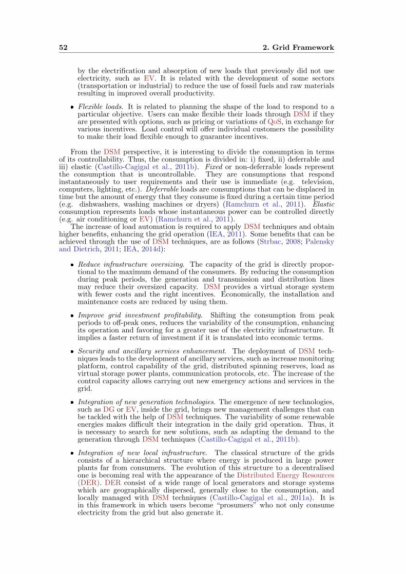
52 2. Grid Framework
by the electrification and absorption of new loads that previously did not useelectricity, such as EV. It is related with the development of some sectors(transportation or industrial) to reduce the use of fossil fuels and raw materialsresulting in improved overall productivity.
Flexible loads. It is related to planning the shape of the load to respond to aparticular objective. Users can make flexible their loads through DSM if theyare presented with options, such as pricing or variations of QoS, in exchange forvarious incentives. Load control will offer individual customers the possibilityto make their load flexible enough to guarantee incentives.
From the DSM perspective, it is interesting to divide the consumption in termsof its controllability. Thus, the consumption is divided in: i) fixed, ii) deferrable andiii) elastic (Castillo-Cagigal et al., 2011b). Fixed or non-deferrable loads representthe consumption that is uncontrollable. They are consumptions that respondinstantaneously to user requirements and their use is immediate (e.g. television,computers, lighting, etc.). Deferrable loads are consumptions that can be displaced intime but the amount of energy that they consume is fixed during a certain time period(e.g. dishwashers, washing machines or dryers) (Ramchurn et al., 2011). Elasticconsumption represents loads whose instantaneous power can be controlled directly(e.g. air conditioning or EV) (Ramchurn et al., 2011).
The increase of load automation is required to apply DSM techniques and obtainhigher benefits, enhancing the grid operation (IEA, 2011). Some benefits that can beachieved through the use of DSM techniques, are as follows (Strbac, 2008; Palenskyand Dietrich, 2011; IEA, 2014d):
Reduce infrastructure oversizing. The capacity of the grid is directly propor-tional to the maximum demand of the consumers. By reducing the consumptionduring peak periods, the generation and transmission and distribution linesmay reduce their oversized capacity. DSM provides a virtual storage systemwith fewer costs and the right incentives. Economically, the installation andmaintenance costs are reduced by using them.
Improve grid investment profitability. Shifting the consumption from peakperiods to off-peak ones, reduces the variability of the consumption, enhancingits operation and favoring for a greater use of the electricity infrastructure. Itimplies a faster return of investment if it is translated into economic terms.
Security and ancillary services enhancement. The deployment of DSM tech-niques leads to the development of ancillary services, such as increase monitoringplatform, control capability of the grid, distributed spinning reserves, load asvirtual storage power plants, communication protocols, etc. The increase of thecontrol capacity allows carrying out new emergency actions and services in thegrid.
Integration of new generation technologies. The emergence of new technologies,such as DG or EV, inside the grid, brings new management challenges that canbe tackled with the help of DSM techniques. The variability of some renewableenergies makes difficult their integration in the daily grid operation. Thus, itis necessary to search for new solutions, such as adapting the demand to thegeneration through DSM techniques (Castillo-Cagigal et al., 2011b).
Integration of new local infrastructure. The classical structure of the gridsconsists of a hierarchical structure where energy is produced in large powerplants far from consumers. The evolution of this structure to a decentralisedone is becoming real with the appearance of the Distributed Energy Resources(DER). DER consist of a wide range of local generators and storage systemswhich are geographically dispersed, generally close to the consumption, andlocally managed with DSM techniques (Castillo-Cagigal et al., 2011a). It isin this framework in which users become “prosumers” who not only consumeelectricity from the grid but also generate it.
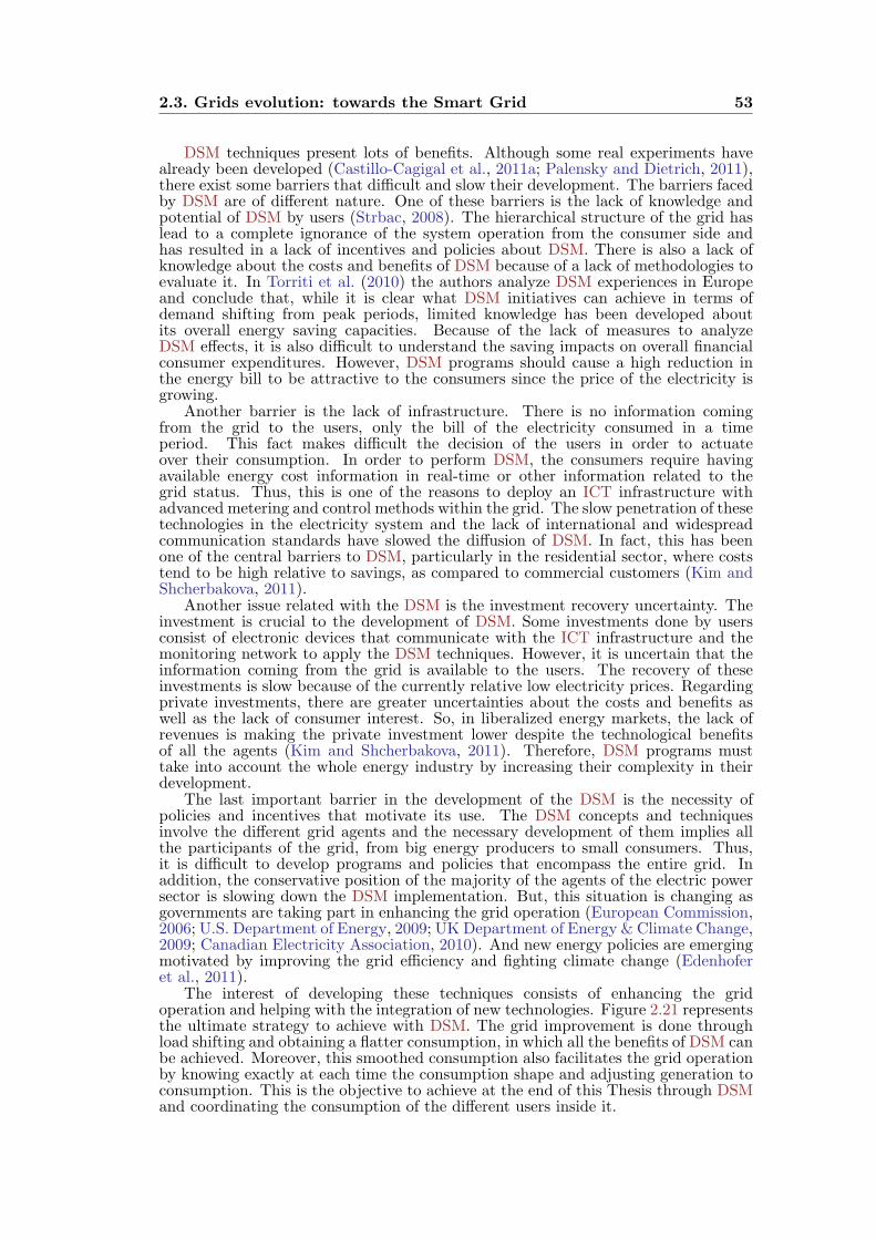
2.3. Grids evolution: towards the Smart Grid 53
DSM techniques present lots of benefits. Although some real experiments havealready been developed (Castillo-Cagigal et al., 2011a; Palensky and Dietrich, 2011),there exist some barriers that difficult and slow their development. The barriers facedby DSM are of different nature. One of these barriers is the lack of knowledge andpotential of DSM by users (Strbac, 2008). The hierarchical structure of the grid haslead to a complete ignorance of the system operation from the consumer side andhas resulted in a lack of incentives and policies about DSM. There is also a lack ofknowledge about the costs and benefits of DSM because of a lack of methodologies toevaluate it. In Torriti et al. (2010) the authors analyze DSM experiences in Europeand conclude that, while it is clear what DSM initiatives can achieve in terms ofdemand shifting from peak periods, limited knowledge has been developed aboutits overall energy saving capacities. Because of the lack of measures to analyzeDSM effects, it is also difficult to understand the saving impacts on overall financialconsumer expenditures. However, DSM programs should cause a high reduction inthe energy bill to be attractive to the consumers since the price of the electricity isgrowing.
Another barrier is the lack of infrastructure. There is no information comingfrom the grid to the users, only the bill of the electricity consumed in a timeperiod. This fact makes difficult the decision of the users in order to actuateover their consumption. In order to perform DSM, the consumers require havingavailable energy cost information in real-time or other information related to thegrid status. Thus, this is one of the reasons to deploy an ICT infrastructure withadvanced metering and control methods within the grid. The slow penetration of thesetechnologies in the electricity system and the lack of international and widespreadcommunication standards have slowed the diffusion of DSM. In fact, this has beenone of the central barriers to DSM, particularly in the residential sector, where coststend to be high relative to savings, as compared to commercial customers (Kim andShcherbakova, 2011).
Another issue related with the DSM is the investment recovery uncertainty. Theinvestment is crucial to the development of DSM. Some investments done by usersconsist of electronic devices that communicate with the ICT infrastructure and themonitoring network to apply the DSM techniques. However, it is uncertain that theinformation coming from the grid is available to the users. The recovery of theseinvestments is slow because of the currently relative low electricity prices. Regardingprivate investments, there are greater uncertainties about the costs and benefits aswell as the lack of consumer interest. So, in liberalized energy markets, the lack ofrevenues is making the private investment lower despite the technological benefitsof all the agents (Kim and Shcherbakova, 2011). Therefore, DSM programs musttake into account the whole energy industry by increasing their complexity in theirdevelopment.
The last important barrier in the development of the DSM is the necessity ofpolicies and incentives that motivate its use. The DSM concepts and techniquesinvolve the different grid agents and the necessary development of them implies allthe participants of the grid, from big energy producers to small consumers. Thus,it is difficult to develop programs and policies that encompass the entire grid. Inaddition, the conservative position of the majority of the agents of the electric powersector is slowing down the DSM implementation. But, this situation is changing asgovernments are taking part in enhancing the grid operation (European Commission,2006; U.S. Department of Energy, 2009; UK Department of Energy & Climate Change,2009; Canadian Electricity Association, 2010). And new energy policies are emergingmotivated by improving the grid efficiency and fighting climate change (Edenhoferet al., 2011).
The interest of developing these techniques consists of enhancing the gridoperation and helping with the integration of new technologies. Figure 2.21 representsthe ultimate strategy to achieve with DSM. The grid improvement is done throughload shifting and obtaining a flatter consumption, in which all the benefits of DSM canbe achieved. Moreover, this smoothed consumption also facilitates the grid operationby knowing exactly at each time the consumption shape and adjusting generation toconsumption. This is the objective to achieve at the end of this Thesis through DSMand coordinating the consumption of the different users inside it.
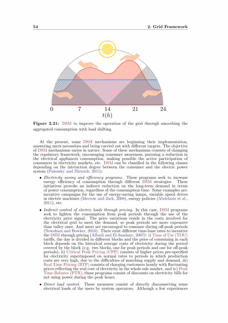
54 2. Grid Framework
0 7 14 21 24t(h)
Figure 2.21: DSM to improve the operation of the grid through smoothing the
aggregated consumption with load shifting.
At the present, some DSM mechanisms are beginning their implementation,answering users necessities and being carried out with different targets. The objectiveof DSM mechanisms varies in nature. Some of these mechanisms consists of changingthe regulatory framework, encouraging consumer awareness, pursuing a reduction inthe electrical appliances consumption, making possible the active participation ofconsumers in electricity markets, etc. DSM can be classified in the following classesdepending on the interaction degree between the consumer and the electric powersystem (Palensky and Dietrich, 2011):
Electricity saving and efficiency programs. These programs seek to increaseenergy efficiency of consumption through different DSM strategies. Theseinitiatives provoke an indirect reduction on the long-term demand in termsof power consumption, regardless of the consumption time. Some examples are:incentive campaigns for the use of energy-saving lamps, variable speed drivesin electric machines (Mecrow and Jack, 2008), energy policies (Abdelaziz et al.,2011), etc.
Indirect control of electric loads through pricing. In this case, DSM programsseek to lighten the consumption from peak periods through the use of theelectricity price signal. The price variations reside in the costs involved forthe electrical grid to meet the demand, so peak periods are more expensivethan valley ones. And users are encouraged to consume during off-peak periods(Newsham and Bowker, 2010). There exist different time-base rates to incentivethe DSM through pricing (Albadi and El-Saadany, 2007): i) Time of Use (TOU)tariffs, the day is divided in different blocks and the price of consuming in eachblock depends on the historical average costs of electricity during the periodcovered by the block (e.g. two blocks, one for peak periods and one for off-peakperiods), ii) Critical Peak Pricing (CPP) consists of higher prices pre-specifiedfor electricity superimposed on normal rates to periods in which productioncosts are very high, due to the difficulties of matching supply and demand, iii)Real Time Pricing (RTP) consists of charging customers hourly with fluctuatingprices reflecting the real cost of electricity in the whole sale market, and iv) PeakTime Rebates (PTR), these programs consist of discounts on electricity bills fornot using power during the peak hours.
Direct load control. These measures consist of directly disconnecting someelectrical loads of the users by system operators. Although a few experiences
2.3. Grids evolution: towards the Smart Grid 55
have been reported with residential consumers, the direct control of loads isusually applied in the industry, controlling large consumers such as foundries(Torriti et al., 2010).
Smart metering and appliances control. These programs make users participantsto control their consumption through market programs or structures that offerload reductions by adapting the demand to the grid status. To do this, it isnecessary that customers have enough information of the grid status and alsoaccess to their consumption to modify it. So, some sophisticated customerscan already tie the electricity pricing into their energy management system.Moreover, these initiatives can achieve greater benefits and greater load shiftsif the price differences between peak and off-peak periods are higher. Thesetechniques require to be accompanied by the application of intelligent appliancesthat facilitate the implementation of DSM (Strbac, 2008).
Continuing with these last incentive programs, new concepts emerge within DSMframework. Hence, the combination of DSM with an automatic control of demandand local generation leads to a new concept called Active Demand Side Management(ADSM) (Castillo-Cagigal et al., 2011a; Matallanas et al., 2012; Masa-Bote et al.,2014). The use of ADSM strategies could benefit firstly to consumers, provided thatthe technologies that implement them automate the operation of devices withoutcompromising the users’ comfort needs and preferences. In the residential sector,there exist lots of possibilities to implement ADSM, since it can be combined withadditional comfort and security functions, improving the demand response, reducingthe environmental impacts (Papagiannis et al., 2008) and offering the user informationabout its electrical consumption. But the residential sector is not the only sectorin which DSM strategies can be applied, for example in the service sector, thecontrol of the air conditioning is being explored in order to implement ADSM.Although ADSM does not directly reduce the amount of energy, the feedback of theconsumption information to the users could reduce the amount of electricity demandedby them (Wood and Newborough, 2003). At present, ADSM strategies are still underdevelopment because it is necessary enough information of local resources (PV orEESs) and the ability to control remotely the different electrical devices to modifythe consumption pattern. In addition, some information coming from the grid suchas its status or the pricing signal are becoming available through the deployment ofthe smart metering.
In conclusion, the benefits of DSM represent a major step towards controlling thedifferent loads of the grid and a considerable improvement in efficiency since it canadapt dynamically the consumption to the generation favoring an enhancement of theoperation of the grid. Thus, the benefits are not only translated in the electricity billsof the user, but also in the environment through the reduction of emissions and otherharmful wastes. In addition, the DSM adds value to the operation of the networksince the development of many SG technologies have been deployed and DSM can helpcontrol power flows without necessarily increase the complexity of the grid operation.In this Thesis, the use of the ADSM helps to integrate the DG and the use of localstorage systems to manage the power flows inside facilities and at the same time toenhance the grid status reducing the variability of the aggregated consumption.

56 2. Grid Framework
3Neural Networks
“Computers deserve to be called intelligent if they could deceive
humans into believing that they were human” — Alan Turing
These days, there exists a growing concern about the use of the dataobtained from different services present in daily live. This is due to thetendency of a society increasingly connected through networks: internet,social (facebook, twitter, etc.), electrical, etc. (Hilbert and Lopez, 2011).
In this context, new concepts arise to extend even more the connectivity to all thedevices and elements that surround us, such as the Internet of Things (IoT) or theSmart Grid (SG). All these applications produce a vast amount of data which bythemselves have no value, but treated properly they can make a difference in thedevelopment of society. The information that resides within these data can be made ofmany kinds: electricity consumption, personal information, interests, mobility alongthe day, location, etc. Thus, if the information is not treated adequately, it can be aburden for the concrete service or application, causing a loss in quality that can leadto a total collapse in the worst case scenario.
Nevertheless, the access to the information that resides within the data is a majorasset to benefit all groups, because it can mean greater operational efficiency, costreductions or reduced risks. Establishing smart relationships between data and userscould enhance the service and offer added value to it, making life more bearable. Thesenew correlations could be the fault preventions in electrical grids, stock prediction inmarkets, combat crime and so on. Therefore, companies are currently developing toolsthat facilitate the acquisition, processing and decision-making of data automatically,through what is known as Big Data Analytics (BDA) (Morabito, 2015). Sometraditional data processing algorithms are inadequate to use with these large datasets due to its complexity and length. BDA has to deal with a few challenges to bedeveloped, such as analysis, capture, share, storage or visualization of the data tounderstand the different relationships among them. Thus, new algorithms are beingdeveloped to analyze these data such as Machine Learning (ML) ones. These type ofalgorithms are oriented to learn from the data and build predictions based on them(Kohavi and Provost, 1998). Normally these algorithms consist of building a modelfrom example data sets and try to generalize them in order to make data-drivenpredictions or decisions, rather than following programmed steps externally (Bishop,2006). There are many approaches of ML, some algorithms used are: decision treelearning, Radial Basis Function (RBF), Support Vector Machine (SVM), PrincipalComponents Analysis (PCA), least-squares optimization, Artificial Neural Network(ANN) and Genetic Algorithm (GA), among others (Marsland, 2009). Most of thealgorithms come from the Artificial Intelligence (AI) field, so that ML is consideredas a branch of AI in charge of handling huge amount of data and extracting featuresfrom them (Blum and Langley, 1997).
But how can these AI algorithms help grids around the world? And why are thesealgorithms particularly interesting to the electrical sector? As described in Chapter 2,the evolution of the electrical grids towards a SG is becoming real. The installation ofan Information and Communications Technology (ICT) infrastructure is generatinglots of data which are necessary to be processed by grid operators, in order to completetheir tasks in a more efficient way. Data processing must be fast enough to makeinstant decisions and effectively use them to take advantage of all the benefits that
58 3. Neural Networks
report the SG (see Section 2.3). However, the grid is currently a centralized systemthat makes difficult to process the vast amount of data generated per minute fromsmart metering. Thus, it will be smart to use some of these techniques, alleviating thedata load from the central node. In addition, the inclusion of these algorithms makesfeasible the decentralization of the system, leaving the decision-making to differentnodes (e.g. substations) within the grid. If decentralization was taken to the end ofthe electricity system (i.e. users who manage their data, process it and take decisionsin order to achieve a common objective), all the parties within the grid would benefitfrom it, being able to overcome all actual problems. In this scenario, nodes couldenhance the system operation, being able to manage their power flows inside the grid.
This Thesis defines a decentralized algorithm to enhance the grid status throughthe management of the power flows inside the users facilities. The use of oneof the classic and more famous AI algorithms is proposed, the ANN, in order tofulfill the objective of enhancing the grid operation by providing decisions to itsmembers. Nowadays, ANNs are enjoying a growing popularity in applications becauseof their features, among which stand out its computing power, decentralized natureand generalization. In addition, through the development of ML techniques andimproving computer hardware, neural structures are increasingly moving towards agreater resemblance to the brain (Eliasmith et al., 2012) or their use in deep learning(Bengio, 2009). In recent years, also biological neural networks have experiencedintense development within the field of the neuroscience (Kandel et al., 2013) and thedevelopment of the technology has made possible to carry out deeper studies.
But why are these algorithms chosen? And why are they suitable to be appliedin the management of a grid? In order to answer these questions, it is necessary tothink in the resemblance between biological neural networks and the electrical ones.Both are large networks that are made up by a lattice of a huge amount of nodesinterconnected. Electricity is present in both networks as the mean to stimulate thenodes, one to produce a reaction in the neuron and the other one to supply thedemand and produce work. The use of ANNs within the grid is very suitable becauseof its distributed properties, adaptability, generalization, redundancy, etc. Propertieswhich are quite similar to the ones that the future SG will provide to conventionalpower systems. ANNs also offers the possibility to establish different hierarchies andsubdivisions to group the nodes, making easy to divide the problem into smallersubtasks. The modularity of the ANNs offer great possibilities to grid operators, bydividing it into portions that are easier to manage by adding more security to thesystem. Moreover, in a scenario in which users become “prosumers” (consumers plusgenerators), the use of ANNs is essential. ANNs provide users with tools to controltheir power flows in order to coordinate with the rest of users like the neurons in thebrain, and to obtain collective benefits for the best grid operation.
The reminder of this Chapter is as follows. A brief historical review is presentedin Section 3.1. Then, what are ANNs and their benefits are explained in Section 3.1.1.The actual tendencies are described in Section 3.1.2. After that, some architectureand types of ANN are introduced in Section 3.2. The type of ANN selected forits application in this Thesis is explained in Section 3.3. Section 3.4 introducesdifferent applications in which ANNs are typically used. Section 3.4.1 will coverthe different implementations of ANN in electrical applications. Finally, Section 3.5explains different forms to train ANNs for the application they were designed for.
3.1 Historical Review
Throughout history, the study of the brain and the nervous system, as well as howhumans can learn and perform tasks, has been the subject of many studies andscholars. In ancient Greek, the first studies on the ideas and the thought weredeveloped by the philosophers Plato (428–348 B.C.) and Aristotle (384–322 B.C.).They together with other ancient Greek philosophers speculated about the causes ofbehavior and the relation of the mind to the brain. On the other hand, there wasno physical interpretation of how the brain and the nervous system were, until thephysician Galen in the 2nd century elaborated his theory. In Galen’s theory, the

3.1. Historical Review 59
nervous system consisted of a lattice of tissue interconnected from the brain to thenerves in the periphery of the body that conveyed fluid secreted by the brain andthe spinal cord (Kandel et al., 2013). However, it was not until the 19th centurythat the actual knowledge of the brain structure was discovered by Ramon y Cajal.He discovered that the nervous system consists of a network of discrete cells, whichwould be called neurons, rather than a continuous web of elements (Ramon y Cajal,1909). During his research, Ramon y Cajal developed a great part of the concepts andevidences for the neuron doctrine, which consists of the principle that the buildingblocks of the brain are the neurons and they are also the signaling elements of thenervous system (Kandel et al., 2013).
At the same time, the belief about artificial beings was also developed sinceantiquity through the mechanical or “formal” reasoning by philosophers and mathe-maticians. The development of the field of logic led to inventions in this area such asthe programmable digital electronic computer. This development was based on theideas of different mathematicians. One of these mathematicians was Alan Turing, whoin 1936 developed a machine called the Turing’s machine that was able to manipulatesymbols and simulate any conceivable act of mathematical deduction (Berlinski,2000). This fact, together with the development of other areas such as informationtheory, neurology and cybernetics allowed the development of a convergence studyof the previous areas known as Artificial Intelligence (AI). This inspired differentresearchers to consider the possibility of building an artificial brain and the race ofArtificial Neural Networks (ANNs) began.
The concept of developing an artificial brain began its first steps with the creationof the neurocomputation in 1943 by Warren S. McCulloch and Walter Pitts. The firstone was a neuroanatomist and psychiatrist, while the second one was a mathematician.They described that any neural network could compute any arithmetic or logicfunction, joining the fields of neurophysiology and mathematical logic (McCullochand Pitts, 1943). They proved that a neural network, consisting of a number ofsimple processing units with proper connections set among them, would perform anyof those functions. This landmark means the beginning of the ANN and the birthof AI through neural computation. The influence of McCulloch and Pitts (1943) wassuch that it inspired von Neumann and Wiener research in von Neumann (1951) andWiener (1948), respectively.
Next milestone in the development of ANN is the publication of the book ofDonald Hebb, entitled The Organization of Behavior (Hebb, 1949). In his book, Hebbexplained the learning process from a psychological perspective and the psychologicalconditioning which is ubiquitous as a property of neurons. The novelty of his workconsisted of the formulation of a learning rule that modifies the synapses of neurons.He proposed that the connections of the brain are changing continuously as differenttasks are learned and neural assemblies are created in those changes. The famousHebb’s rule was introduced in this book and stated that the variance of a synapsebetween two neurons is increased by the activation of one or by the other across itsunion (Hebb, 1949). This rule will influence many researchers from that time untiltoday to elaborate learning synaptic algorithms of ANNs.
During the 50s some interesting events happened that continue the developmentof the ANN such as the construction of the first neurocomputer by Marvin Minsky in1951 called Stochastic Neural Analog Reinforcement Computer (SNARC) (Zurada,1992). SNARC was technically a success, but it did not do any information processingfunction. In addition, different studies during this decade contribute to posteriorachievements: adaptive behavior, nonlinear adaptive filters or works on associativememories (Haykin, 2009). Also, an important event took part in this decade, theDartmouth Conference of 1956.The conference consisted of trying to apply learningaspects to machines and simulate it. This event gave birth to the AI field as it isknown today.
By the end of the 50s, particularly in 1958, the first successful neurocomputer wasdeveloped by Rossenblatt. The perceptron was born and consisted of a supervisedlearning method to the pattern recognition problem (Rosenblatt, 1958). His workwas also known as the perceptron convergence theorem and it was himself the firstone to prove its validity. The perceptron was the first ANN able to generalize, i.e.after learning a set of patterns, it could recognize similar ones that were never used
60 3. Neural Networks
during the learning phase. Then, Widrow and Hoff developed a new algorithm calledLeast Mean Squares (LMS), which was the pillar to build the ADAptative LINearElements (ADALINE) (Widrow and Hoff, 1960). Nowadays, this algorithm is still inuse, unlike the perceptron learning law. The ADALINE was applied in a real problemas adaptive filter to eliminate the echoes in telephonic lines. It also inspired the use ofother more complex structures, such as the Multiple ADALINE, and other stochasticlearning algorithms to be applied to ANNs.
With these events, it seemed in the 60s that ANNs were the solution to all theproblems, prove of that is the wide research done in the field and the number ofapplications in which ANNs were employed. However, this glorious era came toan end with Minsky and Papert (1969). Perceptron limitations were highlighted inthis book. They proved that single layer perceptrons cannot compute non linearfunctions and doubted that multilayer perceptrons or any other structure could solvethis problem. They left the impression that the research in this field was a dead end.In addition, another reason that favored the abandon of many researchers was thelack of technological devices to carry out experiments.
During the 70s, the research of ANNs seemed to be dead, but some psychologistsand neuroscientists continued the research in the field, focused on adaptive signalprocessing, pattern recognition and biological modeling. In (Amari, 1972), thelearning in ANNs with thresholds was studied and he developed a stochastic gradientmethod. Stephen Grossberg developed different ANN structures and theories aboutadaptive resonance networks (Grossberg, 1974). These theories consisted of a newprinciple of self-organization with a recognition layer and a generative layer. At thesame time, the inception of what later became one of the widespread algorithms,the backpropagation algorithm, was developed by Werbos (1974). In his thesis, PaulWerbos applied successfully an efficient reverse-mode gradient computation that wasapplied to general networks. Associative memory research was also developed in thisdecade and the studies in self-organization continued in Kohonen (1977). KunihikoFukushima developed another neural structure known as neocognitron (Fukushima,1980). This structure consisted of a model that emulates the retinal image of theneurons trying to solve problems of visual pattern recognition. These researchers andmany others in this decade were the people who prepared the ANNs to their nextstep and help to develop the base of the new achievements found in the next years.
Then in the 80s a renaissance era began for the study of ANN. Hopfield (1982)supposed a turning point in between the dormancy of the 70s and the beginningof a renewed enthusiasm on ANN. The work of Hopfield consisted in the study ofrecurrent structures with symmetric connections using the idea of an energy functionto understand the way in which this structure computes the information. Hopfield(1982) encouraged hundreds of scientists, mathematicians, and technologists to rejointhe emerging field of neural networks. Another milestone that influenced this era wasthe publication of Rumelhart and McClelland (1986), which used the backpropagationalgorithm to train multilayer perceptrons. Formally, the backpropagation algorithmwas formulated at mid 80s, but it was first described in the work of Werbos(1974). These two publications led to the resurgence of the ANN field to exploreneurocomputation. In the following years, the ANN increased significantly itsexpansion with the foundation of the International Neural Network Society, a journalto publish the research work in this field, IEEE Transactions on Neural Networks anddifferent conferences such as the IEEE International Conference on Neural Networks.
This era will support the ANN expansion in the upcoming years of the 90s. Theresearch on structures, learning algorithms and self-organizing methods will continueto develop, such as the Radial Basis Function (RBF) that consisted of a feedforwardnetwork alternative to perceptrons, or the Support Vector Machine (SVM) consistingon a supervised learning network to solve pattern recognition and regression problems.However, there was also an expansion to use these algorithms in other fields such ascontrol, prediction and finance, taking advantage of the many qualities that suchstructures have. Also, during this time a concern about the dynamics of ANNs roseamong researchers. Freeman (1995) tried to explain the existence of chaotic behaviorsin neural structures and the emergence of self-organized patterns in populations ofneurons. Furthermore, the advance of the technology in this decade allowed buildingspecific hardware to compute the operation of an ANN. Thus, the operation of the
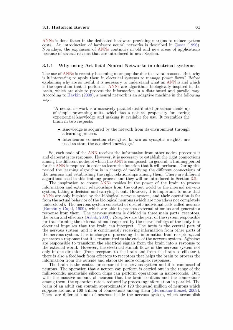
3.1. Historical Review 61
ANNs is done faster in the dedicated hardware providing margins to reduce systemcosts. An introduction of hardware neural networks is described in Goser (1996).Nowadays, the expansion of ANNs continues in old and new areas of applicationsbecause of several reasons that are introduced in next Section.
3.1.1 Why using Artificial Neural Networks in electrical systems
The use of ANNs is recently becoming more popular due to several reasons. But, whyis it interesting to apply them in electrical systems to manage power flows? Beforeexplaining why are so useful, it is necessary to understand what an ANN is and whichis the operation that it performs. ANNs are algorithms biologically inspired in thebrain, which are able to process the information in a distributed and parallel way.According to Haykin (2009), a neural network is an adaptive machine in the followingway:
“A neural network is a massively parallel distributed processor made upof simple processing units, which has a natural propensity for storingexperiential knowledge and making it available for use. It resembles thebrain in two respects:
Knowledge is acquired by the network from its environment througha learning process.
Interneuron connection strengths, known as synaptic weights, areused to store the acquired knowledge.”
So, each node of the ANN receives the information from other nodes, processes itand elaborates its response. However, it is necessary to establish the right connectionsamong the different nodes of which the ANN is composed. In general, a training periodfor the ANN is required in order to learn the function that it will perform. During thisperiod the learning algorithm is in charge of modifying the different connections ofthe neurons and establishing the right relationships among them. There are differentalgorithms used in this training process and they will be introduced in Section 3.5.
The inspiration to create ANNs resides in the power of the brain to processinformation and extract relationships from the output world to the internal nervoussystem, taking a decision and carrying it out. However, it is important to note thatANNs are only inspired by the biological nervous system, and their operation is farfrom the actual behavior of the biological neurons (which are nowadays not completelyunderstood). The nervous system consisted of discrete individual cells called neurons(Ramon y Cajal, 1909), which are able to process external stimulus and generate aresponse from them. The nervous system is divided in three main parts, receptors,the brain and effectors (Arbib, 2003). Receptors are the part of the system responsiblefor transforming the external stimuli captured by the nerve endings of the body intoelectrical impulses that the brain can interpret. The brain is the central part ofthe nervous system, and it is continuously receiving information from other parts ofthe nervous system. It is in charge of processing the information from receptors, andgenerates a response that it is transmitted to the ends of the nervous system. Effectorsare responsible to transform the electrical signals from the brain into a response tothe external world. However, the electrical stimuli flows in the nervous system notonly in one direction (from receptors to the brain and from the brain to effectors),there is also a feedback from effectors to receptors that helps the brain to process theinformation from the outside and elaborate more complex responses.
The brain is the central processor of the nervous system and it is composed ofneurons. The operation that a neuron can perform is carried out in the range of themilliseconds, meanwhile silicon chips can perform operations in nanoseconds. But,with the massive amount of neurons that the brain contains and the connectionsamong them, the operation rate is reduced by processing information in parallel. Thebrain of an adult can contain approximately 120 thousand million of neurons whichsuppose around a 100 trillion of connections among them (Herculano-Houzel, 2009).There are different kinds of neurons inside the nervous system, which accomplish
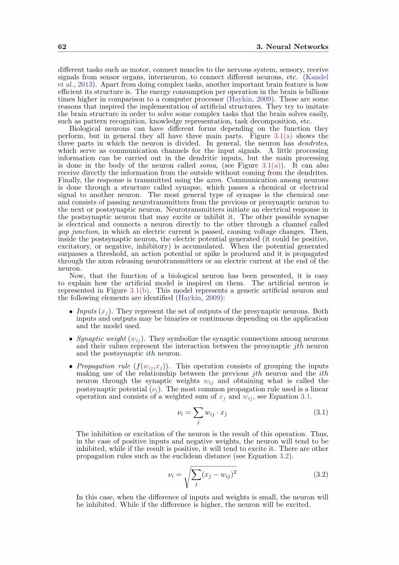
62 3. Neural Networks
different tasks such as motor, connect muscles to the nervous system, sensory, receivesignals from sensor organs, interneuron, to connect different neurons, etc. (Kandelet al., 2013). Apart from doing complex tasks, another important brain feature is howefficient its structure is. The energy consumption per operation in the brain is billionstimes higher in comparison to a computer processor (Haykin, 2009). These are somereasons that inspired the implementation of artificial structures. They try to imitatethe brain structure in order to solve some complex tasks that the brain solves easily,such as pattern recognition, knowledge representation, task decomposition, etc.
Biological neurons can have different forms depending on the function theyperform, but in general they all have three main parts. Figure 3.1(a) shows thethree parts in which the neuron is divided. In general, the neuron has dendrites,which serve as communication channels for the input signals. A little processinginformation can be carried out in the dendritic inputs, but the main processingis done in the body of the neuron called soma, (see Figure 3.1(a)). It can alsoreceive directly the information from the outside without coming from the dendrites.Finally, the response is transmitted using the axon. Communication among neuronsis done through a structure called synapse, which passes a chemical or electricalsignal to another neuron. The most general type of synapse is the chemical oneand consists of passing neurotransmitters from the previous or presynaptic neuron tothe next or postsynaptic neuron. Neurotransmitters initiate an electrical response inthe postsynaptic neuron that may excite or inhibit it. The other possible synapseis electrical and connects a neuron directly to the other through a channel calledgap junction, in which an electric current is passed, causing voltage changes. Then,inside the postsynaptic neuron, the electric potential generated (it could be positive,excitatory, or negative, inhibitory) is accumulated. When the potential generatedsurpasses a threshold, an action potential or spike is produced and it is propagatedthrough the axon releasing neurotransmitters or an electric current at the end of theneuron.
Now, that the function of a biological neuron has been presented, it is easyto explain how the artificial model is inspired on them. The artificial neuron isrepresented in Figure 3.1(b). This model represents a generic artificial neuron andthe following elements are identified (Haykin, 2009):
Inputs (xj). They represent the set of outputs of the presynaptic neurons. Bothinputs and outputs may be binaries or continuous depending on the applicationand the model used.
Synaptic weight (wij). They symbolize the synaptic connections among neuronsand their values represent the interaction between the presynaptic jth neuronand the postsynaptic ith neuron.
Propagation rule (f(wij ,xj)). This operation consists of grouping the inputsmaking use of the relationship between the previous jth neuron and the ithneuron through the synaptic weights wij and obtaining what is called thepostsynaptic potential (νi). The most common propagation rule used is a linearoperation and consists of a weighted sum of xj and wij , see Equation 3.1.
νi =∑j
wij · xj (3.1)
The inhibition or excitation of the neuron is the result of this operation. Thus,in the case of positive inputs and negative weights, the neuron will tend to beinhibited, while if the result is positive, it will tend to excite it. There are otherpropagation rules such as the euclidean distance (see Equation 3.2).
νi =
√∑j
(xj − wij)2 (3.2)
In this case, when the difference of inputs and weights is small, the neuron willbe inhibited. While if the difference is higher, the neuron will be excited.
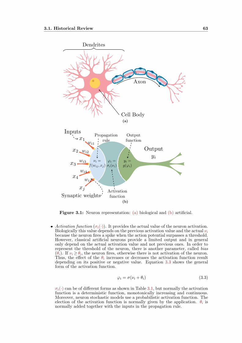
3.1. Historical Review 63
Axon
Cell Body
Dendrites
(a)
Inputsx1
x2
x3
x4
xj
Outputyi
yi =g(ϕi)
ϕi =σi(νi)
νi =f(wij , xj)
Synaptic weights
wi1
wi2
wi3
wi4
wij
Propagationrule
Activationfunction
Outputfunction
(b)
Figure 3.1: Neuron representation: (a) biological and (b) artificial.
Activation function (σi(·)). It provides the actual value of the neuron activation.Biologically this value depends on the previous activation value and the actual νibecause the neuron fires a spike when the action potential surpasses a threshold.However, classical artificial neurons provide a limited output and in generalonly depend on the actual activation value and not previous ones. In order torepresent the threshold of the neuron, there is another parameter, called bias(θi). If νi≥ θi, the neuron fires, otherwise there is not activation of the neuron.Thus, the effect of the θi increases or decreases the activation function resultdepending on its positive or negative value. Equation 3.3 shows the generalform of the activation function.
φi = σ(νi + θi) (3.3)
σi(·) can be of different forms as shown in Table 3.1, but normally the activationfunction is a deterministic function, monotonically increasing and continuous.Moreover, neuron stochastic models use a probabilistic activation function. Theelection of the activation function is normally given by the application. θi isnormally added together with the inputs in the propagation rule.
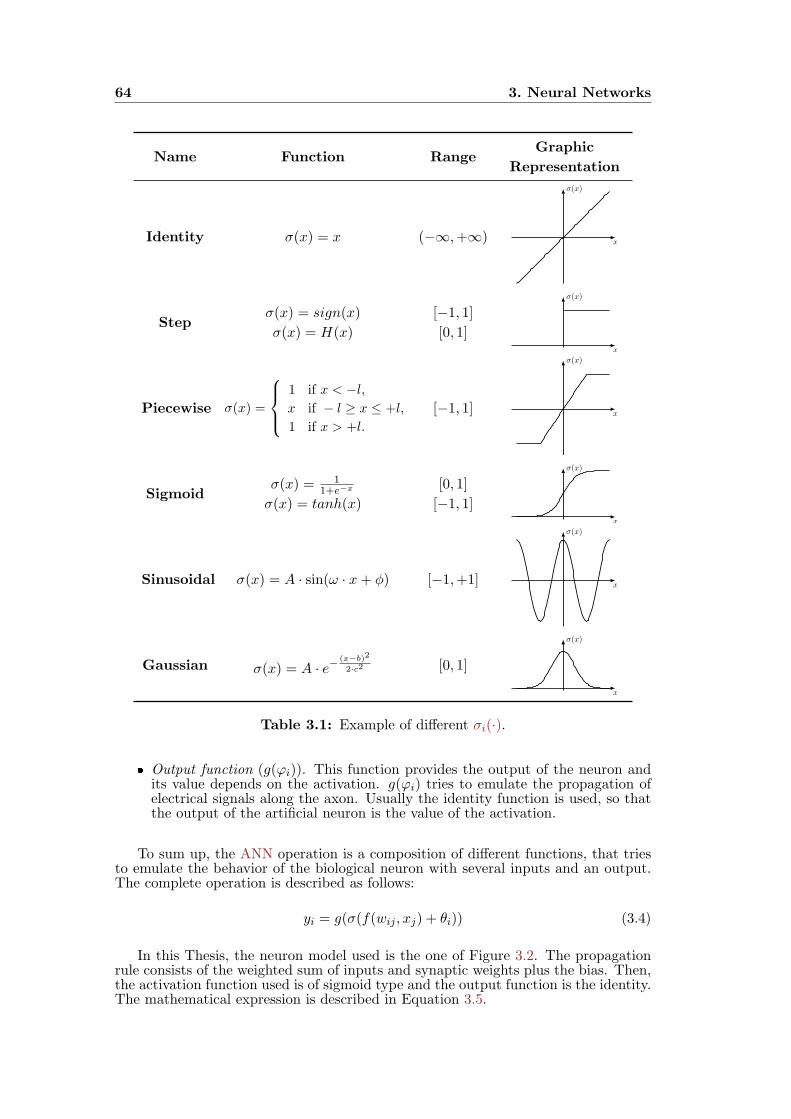
64 3. Neural Networks
Name Function RangeGraphic
Representation
Identity σ(x) = x (−∞,+∞)x
σ(x)
Stepσ(x) = sign(x)
σ(x) = H(x)
[−1, 1][0, 1]
x
σ(x)
Piecewise σ(x) =
1 if x < −l,x if − l ≥ x ≤ +l,
1 if x > +l.
[−1, 1]x
σ(x)
Sigmoidσ(x) = 1
1+e−x
σ(x) = tanh(x)
[0, 1]
[−1, 1]x
σ(x)
Sinusoidal σ(x) = A · sin(ω · x+ ϕ) [−1,+1]x
σ(x)
Gaussian σ(x) = A · e−(x−b)2
2·c2 [0, 1]
x
σ(x)
Table 3.1: Example of different σi(·).
Output function (g(φi)). This function provides the output of the neuron andits value depends on the activation. g(φi) tries to emulate the propagation ofelectrical signals along the axon. Usually the identity function is used, so thatthe output of the artificial neuron is the value of the activation.
To sum up, the ANN operation is a composition of different functions, that triesto emulate the behavior of the biological neuron with several inputs and an output.The complete operation is described as follows:
yi = g(σ(f(wij , xj) + θi)) (3.4)
In this Thesis, the neuron model used is the one of Figure 3.2. The propagationrule consists of the weighted sum of inputs and synaptic weights plus the bias. Then,the activation function used is of sigmoid type and the output function is the identity.The mathematical expression is described in Equation 3.5.
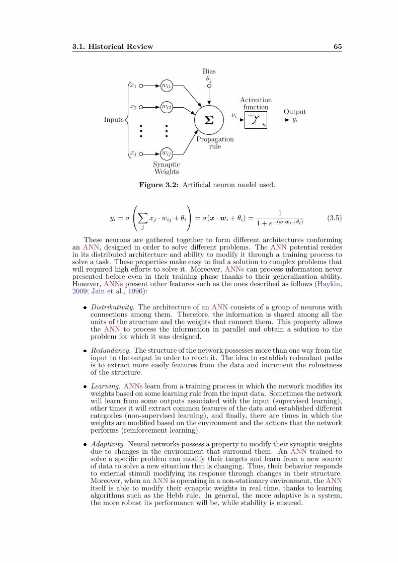
3.1. Historical Review 65
Σ
Propagationrule
wi1x1
wi2x2
wij
SynapticWeights
xj
Biasθj
Inputsνi
σ(νi)νi
Activationfunction
Outputyi
Figure 3.2: Artificial neuron model used.
yi = σ
∑j
xj · wij + θi
= σ(x ·wi + θi) =1
1 + e−(x·wi+θi)(3.5)
These neurons are gathered together to form different architectures conformingan ANN, designed in order to solve different problems. The ANN potential residesin its distributed architecture and ability to modify it through a training process tosolve a task. These properties make easy to find a solution to complex problems thatwill required high efforts to solve it. Moreover, ANNs can process information neverpresented before even in their training phase thanks to their generalization ability.However, ANNs present other features such as the ones described as follows (Haykin,2009; Jain et al., 1996):
Distributivity. The architecture of an ANN consists of a group of neurons withconnections among them. Therefore, the information is shared among all theunits of the structure and the weights that connect them. This property allowsthe ANN to process the information in parallel and obtain a solution to theproblem for which it was designed.
Redundancy. The structure of the network possesses more than one way from theinput to the output in order to reach it. The idea to establish redundant pathsis to extract more easily features from the data and increment the robustnessof the structure.
Learning. ANNs learn from a training process in which the network modifies itsweights based on some learning rule from the input data. Sometimes the networkwill learn from some outputs associated with the input (supervised learning),other times it will extract common features of the data and established differentcategories (non-supervised learning), and finally, there are times in which theweights are modified based on the environment and the actions that the networkperforms (reinforcement learning).
Adaptivity. Neural networks possess a property to modify their synaptic weightsdue to changes in the environment that surround them. An ANN trained tosolve a specific problem can modify their targets and learn from a new sourceof data to solve a new situation that is changing. Thus, their behavior respondsto external stimuli modifying its response through changes in their structure.Moreover, when an ANN is operating in a non-stationary environment, the ANNitself is able to modify their synaptic weights in real time, thanks to learningalgorithms such as the Hebb rule. In general, the more adaptive is a system,the more robust its performance will be, while stability is ensured.

66 3. Neural Networks
Generalization. Once the network is trained with a dataset, the network isnormally executed with more data that was not presented in first place to thenetwork during the training. If the ANN was able to extract the main featuresof the dataset, it will be able to generalize and obtain a right answer for otherdatasets. Otherwise, the ANN would not be able to generalize and obtain theinformation from the new data.
Non linear operation. A neuron could be linear or nonlinear depending on theσi(·) selected. In turn, the ANN, built with these neurons, may inherit thesame nature of the neurons which form part of it. In addition, the nonlinearityis distributed through the whole network. The importance of this feature isthat an ANN can be used to solve nonlinear problems, such as the predictionof electricity generation and demand, or simulate the dynamics of a complexsystem like the grid.
Input-output mapping. Some ANNs are able to learn through the environmentin a training stage that consists of modifying the synaptic weights. Thismodification varies the weights in order to obtain the right output that it isalso provided as part of the training. Each example is composed of the tupleof inputs and outputs, arranged randomly. So, the ANN is able to extract arelationship between the outputs and inputs presented during the training. Inthis way, when the network is presented with a new input never trained, it hasto be able to solve the problem with a right answer.
Multi objective output. The response of an ANN can be of different nature,being able to obtain different information at the same time from one input. Forexample, in a pattern recognition application, an ANN can be designed to selecta pattern and at the same time the confidence in the made selection. So, anANN can be built with the outputs needed to develop different tasks.
Contextual information. The knowledge of the ANN is represented by differentelements that form its structure and their activation. Each neuron within theANN is affected by the overall activity of the other neurons.
Fault tolerance. This is another built-in property of the ANN because of thestructure distributivity. The knowledge is stored through the whole structure.If a connection fails, the information is rerouted to other parts of the networkand it can continue giving a response. In spite of loosing a part of the structure,the network structure is robust.
Task decomposition. Thanks to the information distributivity inside thenetwork, it is easy to build small structures that solve parts of the problem.Then, the result of each part of the problem is integrated into a more complexresponse to solve the task to which it was built in first place. This propertymakes possible the simplification of the problem and also simplifies the structureof the network.
Analysis and design uniformity. In spite of the different applications andstructures of the ANNs, there exist some conventions in their design. Forexample, the notation is the same for different applications. All ANNs areformed by neurons, so that different theories and learning algorithms can beshared for different applications.
Low energy consumption. Because of its massive parallelism computing capacity,ANNs are very efficient and the electricity consumed in each operation by unit isreally small compared to other computation structures. This property facilitatestheir integration in those applications in which energy is a problem, but a highprocessing capacity is required.
ANNs present lots of benefits that make them useful for almost any application.However, they also present some difficulties related to its structure. One of the
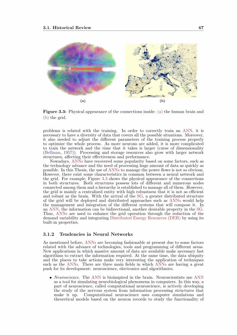
3.1. Historical Review 67
(a) (b)
Figure 3.3: Physical appearance of the connections inside: (a) the human brain and
(b) the grid.
problems is related with the training. In order to correctly train an ANN, it isnecessary to have a diversity of data that covers all the possible situations. Moreover,it also needed to adjust the different parameters of the training process properlyto optimize the whole process. As more neurons are added, it is more complicatedto train the network and the time that it takes is larger (curse of dimensionality(Bellman, 1957)). Processing and storage resources also grow with larger networkstructures, affecting their effectiveness and performance.
Nowadays, ANNs have recovered some popularity based on some factors, such asthe technology advance and the need of processing huge amount of data as quickly aspossible. In this Thesis, the use of ANNs to manage the power flows is not so obvious.However, there exist some characteristics in common between a neural network andthe grid. For example, Figure 3.3 shows the physical appearance of the connectionsin both structures. Both structures possess lots of different and numerous nodesconnected among them and a hierarchy is established to manage all of them. However,the grid is mainly a centralized entity with high robustness that it is not as efficientand robust as the brain. With the arrival of the SG, a greater distributed structureof the grid will be deployed and distributed approaches such as ANNs would helpthe management and integration of the different systems that will compose it. Inan ANN, the information can be bidirectional, another desirable property in the SG.Thus, ANNs are used to enhance the grid operation through the reduction of thedemand variability and integrating Distributed Energy Resources (DER) by using itsbuilt-in properties.
3.1.2 Tendencies in Neural Networks
As mentioned before, ANNs are becoming fashionable at present due to some factorsrelated with the advance of technologies, tools and programming of different areas.New applications in which massive amount of data are available make necessary fastalgorithms to extract the information required. At the same time, the data ubiquityand the places to take actions make very interesting the application of techniquessuch as the ANNs. There are three main fields in which ANNs are having a greatpush for its development: neuroscience, electronics and algorithmics.
Neuroscience. The ANN is bioinspired in the brain. Neuroscientists use ANNas a tool for simulating neurobiological phenomena in computers. In this way, apart of neuroscience, called computational neuroscience, is actively developingthe study of the nervous system from information processing structures thatmake it up. Computational neuroscience uses computer simulations andtheoretical models based on the neuron records to study the functionality of
68 3. Neural Networks
each part of the nervous system (Dayan and Abbott, 2001). There exist differentmodels that represent different aspects of the neural systems and the degree ofabstraction is different for each of them depending on the brain area studied.In general, the neuron model used in computational neuroscience is a spikingneuron. The spiking model consists of a more realistic biological model of aneuron. In this case, the time is added to the other components of previousmodels, activation state and synaptic weights. This model considers the electriccurrent that circulates inside the neuron and the potential that it creates,modeled as a differential equation. Thus, a spiking neuron only fires whenits activation potential reaches a specific value, and then a relaxation period ofthe activation is necessary for the neuron to fire again. The neuron, which hasfired a spike, generates a signal to the rest of neurons that are connected toit, increasing or decreasing their potential depending on the signal (Dayan andAbbott, 2001).The spikes train of a population of neurons is then encoded so that theinformation is easier to interpret. And with this information the model isbuilt to simulate the concrete part of the brain that the neuroscientists wantto analyze. Therefore, the idea of these models is to convert the informationof the external world of the brain to the neural space through the encoding ofthe spikes train generated by the stimuli of a neuron population. Then, a seriesof transformations are done with the encoded spikes and finally translated outof the neural space by another population of neurons to understand from theoutside of the neural model the actions that have been taken place inside.One tool that is gaining prominence within the neural simulation scene is theNeural Engineering Framework (NEF). Its novelty resides in the characteriza-tion of population-temporal coding that combines population vectors with lineardecoding of neural spikes. This framework is based on signal processing andstatistical inference, providing a robust strategy and evaluating the functionof a wide variety of specific neural circuits. NEF is currently being appliedto sensory processing, motor control and cognitive function (Eliasmith andAnderson, 2003). This framework consists of three principles:
i) Representation. The representation principle consists of how the informa-tion is coded and decoded inside the neural space for the neuron population.The encoding of the input information is nonlinear while the decoding usedin the output neuron population is linear.
ii) Transformation. Transformation of neural representations are functionsof variables represented by the different populations of neurons. Thistransformation is applied by a weighted linear decoding into the outputpopulation.
iii) Dynamics. And finally, the last principle consists of applying controltheory to simulate neural representation dynamics for the different neuronpopulations.
NEF provides an easy way to encode and decode populations of neurons,control theory as a way to simulate their dynamics, a general way to generateneural systems with analytical synaptic weights for the functionality desired andpromotes the formulation of specific hypotheses about circuit functions and keydesign constraints (Eliasmith and Anderson, 2003).With NEF, the first working computational simulation of the brain hasbeen implemented in Eliasmith et al. (2012), and is known as SemanticPointer Architecture Unified Network (SPAUN). SPAUN is able to carryout about 8 cognitive and non-cognitive tasks that can be integrated in asingle large-scale spiking neuron model. It is able to develop the followingtasks: recognition, drawing, reinforcement learning, counting, working memory,answering questions, create variables and reasoning. SPAUN is able to switchbetween the different tasks automatically without any manual change in theroutines of the programs. Thus, it is a fixed model that integrates perception,cognition, and action across several tasks.In the race to the brain simulation, there are other projects that try to emulate
3.1. Historical Review 69
the brain functioning by simulating each of the different neurons of the brainand putting them together, so that they can do the same tasks as a humanbrain1. Another interesting project is the Human Connectome Project, whichaims at studying the connections among neurons in the brain trying to elaboratean atlas of the different parts of the brain2. Both projects contribute to have abetter understanding of how the brain works, but they are not implementing afunctional model that completes tasks from an AI point of view such as SPAUN.As mentioned before, NEF applies control theory to understand the dynamicsof the neural models. However, there is another aspect inside neurosciencethat tries to directly study the neurons and the association between them asdynamical systems (Izhikevich, 2007). In this case the idea is to explain neuralmodels through the dynamics of spiking neurons and observe the behavior thatcomes from their interactions to explain how a neural ensemble works. InIzhikevich (2007), the nonlinear dynamics systems of the brain are explained,beginning from a low dimensional neural space to a higher one.
Electronics. The next field in which ANNs are having important advances isin hardware for their implementation and neuromorphic computers. This ideais gaining more followers because technology is mature enough to implementdirectly the ANN behavior at an affordable cost. In addition, the costs decreaseas volume production increases, so it could be interesting to adopt a specifichardware in case the application volume is higher. Another advantage ofhardware implementation is the increase of speed since the neural operationis dedicated. There are many classes of hardware used to implement ANNs(Misra and Saha, 2010):
– Digital chips consist of specific hardware dedicated to emulate neurons, ingeneral they use CMOS technology and store the weights in RAM, whichallow a flexible design.
– An analog neuron is emulated in hardware through resistors, charge-coupled devices, capacitors, etc. Thus, the hardware itself implementsthe neuron structure, being the design more rigid than digital one.
– Field Programmable Gate Arrays (FPGAs) provide an effective way toprogram different neural structures through their reconfigurable structurein a very short time and with low costs. It provides software flexibility andonline reconfiguration capabilities (Misra and Saha, 2010).
– Fast Graphics Processing Unit (GPU)-based implementations of ANNs arealso being used to emulate large structures because as FPGAs, they allowreconfiguring rapidly the structure and the computation capacity is higherthan CPU implementations.
– The chips that are currently having greater development are the neuro-morphic ones. Neuromorphic refers to circuits that emulate closely thebiological neural design. Almost all the processing is analog, but theiroutputs can be digital. An example of neuromorphic chip is the Neurogriddeveloped in Benjamin et al. (2014). The board is composed of 16custom-designed chips, referred to as NeuroCores. NeuroCore analog partconsisted of the emulation of 65536 neurons trying to maximize the energyefficiency. The emulated neurons are connected using digital circuitrydesigned to maximize spiking throughput.
Algorithmcs. As technologies and models advance, they allow spreading thefields of application in which ANNs can actuate. This is reason why the ANNstructure can be further complicated by adding more neurons and using morecomplex hierarchies with more elements. At present, ANNs are being used inMachine Learning (ML) algorithms as one of the principal techniques due to thenonlinearity operation and the possibility to establish easy relationships among
1Blue Brain Project official website: http://bluebrain.epfl.ch/2Human Connectome official website: http://humanconnectome.org/

70 3. Neural Networks
Neuron Layer Network System
Σ σ(·)
x1
x2
x3
x4
x5
yi
N1
y1
x1
N2
y2
x2
N3
y3
x3
N4
y4
N1
x1
N2
x2
N3
x3
N4
N5
y5
N6
y6
ProcessingAlgorithm
NeuralNetwork
Inputsx
Σ
+
−
ei
di
yi
ProcessingAlgorithm
NeuralNetwork
Σ
Figure 3.4: Different association of neurons to form different structures.
massive quantities of data. Another interesting ability for ML is elaboratinggeneral purpose predictions based on the data available, in which ANN standsout (Blum and Langley, 1997). In addition, the ANN feature extraction hasbeen improved due to the increasing complexity of the network structure, beingable to process not only lager datasets, but also fast enough to consider it as apromising algorithm to take into account.As mentioned before, neuroscientist looks into ANNs as a research tool toimplement neurobiological models. However, engineers also seek in neurobiologyfor new ideas to solve more complex problems. That is how Deep Learning(DL) arises in the actual scene of ANNs. This allows implementing networkarchitectures that can be used for example in the vision recognition problems.In this case, the structure of DL-ANN consists of more neurons in thenetwork, more connections among them and a deeper hierarchy with a greaterresemblance to the human brain. One application in which these complexarchitectures are used is in computer vision in which convolutional ANNs areused (Krizhevsky et al., 2012). The idea of this structure is building differentlayers of neurons in which the feature extraction is done. A convolutionalnetwork is a type of ANN in which neurons are tiled in such a way that theyrespond to overlapping regions in the visual field. Google has also developedhis own version of them, GoogLeNet (Szegedy et al., 2015). Furthermore, inLe et al. (2012), the authors uses a DL architecture that learned to recognizehigher-level concepts only from watching unlabeled images. Other structure forfeature extraction is the autoencoder, which tries to compress the informationfrom a higher dimensional space to a smaller one that contains the main featuresfrom the previous one. Therefore, the complexity of new applications is evolvingthe concepts around ANNs and developing new models with major proximityto the theoretic goals of AI.
3.2 Architectures and Types
So far the principles, history and future of the ANNs have been introduced. Inthis Section, different types, architectures and structures are introduced. The basicbuilding block of ANNs is the neuron and it is used as a small processing unit. Aset of neurons is usually grouped forming layers which have its own functionality.Then, the different layers are also grouped together to form a global system, knownas neural network. In addition, various neural networks can be associated to form aneural system, which is able to complete a specific task (see Figure 3.4). Both conceptscould be applied in biological and artificial contexts. In an ANN, the different modulesin which the system is divided do not have to be neural. Thus, an artificial system inwhich an ANN is taking part consists of inputs that go to the corresponding moduleswhere the information is processed and then the system output is obtained to solvethe task for which was built.
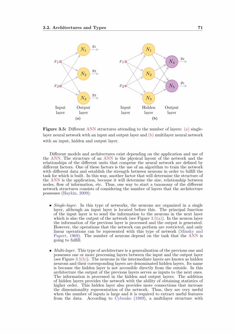
3.2. Architectures and Types 71
N1
y1
x1
N2
y2
x2
N3
y3
Input
layer
Output
layer
(a)
N1
x1
N2
x2
N3
N4
y4
N5
y5
Input
layer
Hidden
layer
Output
layer
(b)
Figure 3.5: Different ANN structures attending to the number of layers: (a) single-
layer neural network with an input and output layer and (b) multilayer neural network
with an input, hidden and output layer.
Different models and architectures exist depending on the application and use ofthe ANN. The structure of an ANN is the physical layout of the network and therelationships of the different units that comprise the neural network are defined bydifferent factors. One of these factors is the use of an algorithm to train the networkwith different data and establish the strength between neurons in order to fulfill thetask for which is built. In this way, another factor that will determine the structure ofthe ANN is the application, because it will determine the size, relationship betweennodes, flow of information, etc. Thus, one way to start a taxonomy of the differentnetwork structures consists of considering the number of layers that the architecturepossesses (Haykin, 2009):
Single-layer. In this type of networks, the neurons are organized in a singlelayer, although an input layer is located before this. The principal functionof the input layer is to send the information to the neurons in the next layerwhich is also the output of the network (see Figure 3.5(a)). In the neuron layerthe information of the previous layer is processed and the output is generated.However, the operations that the network can perform are restricted, and onlylinear operations can be represented with this type of network (Minsky andPapert, 1969). The number of neurons depend on the task that the ANN isgoing to fulfill.
Multi-layer. This type of architecture is a generalization of the previous one andpossesses one or more processing layers between the input and the output layer(see Figure 3.5(b)). The neurons in the intermediate layers are known as hiddenneurons and their corresponding layers are denominated hidden layers. Its nameis because the hidden layer is not accessible directly from the outside. In thisarchitecture the output of the previous layers serves as inputs to the next ones.The information is processed in the hidden and output layers. The additionof hidden layers provides the network with the ability of obtaining statistics ofhigher order. This hidden layer also provides more connections that increasethe dimensionality representation of the network. Thus, they are very usefulwhen the number of inputs is large and it is required to extract useful featuresfrom the data. According to Cybenko (1989), a multilayer structure with
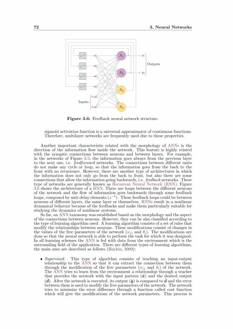
72 3. Neural Networks
N1y1z−1
N2y2
z−1
N3
z−1
N4
z−1
x1
x2
Inputs
Outputs
Figure 3.6: Feedback neural network structure.
sigmoid activation function is a universal approximator of continuous functions.Therefore, multilayer networks are frequently used due to these properties.
Another important characteristic related with the morphology of ANNs is thedirection of the information flow inside the network. This feature is highly relatedwith the synaptic connections between neurons and between layers. For example,in the networks of Figure 3.5, the information goes always from the previous layerto the next one, i.e. feedforward networks. The connections between different unitsdo not make any cycle or loop, so that the information goes from the back to thefront with no recurrence. However, there are another type of architectures in whichthe information does not only go from the back to front, but also there are someconnections that allow the information going backwards, i.e. feedback networks. Thesetype of networks are generally known as Recurrent Neural Network (RNN). Figure3.6 shows the architecture of a RNN. There are loops between the different neuronsof the network and the flow of information goes backwards through some feedbackloops, composed by unit-delay elements (z−1). These feedback loops could be betweenneurons of different layers, the same layer or themselves. RNNs result in a nonlineardynamical behavior because of the feedbacks and make them particularly suitable forstudying the dynamics of nonlinear systems.
So far, an ANN taxonomy was established based on the morphology and the aspectof the connections between neurons. However, they can be also classified according tothe type of learning algorithm used. A learning algorithm consists of a set of rules thatmodify the relationships between neurons. These modifications consist of changes inthe values of the free parameters of the network (wij and θi). The modifications aredone so that the neural network is able to perform the task for which it was designed.In all learning schemes the ANN is fed with data from the environment which is thesurrounding field of the application. There are different types of learning algorithms,the main ones are described as follows (Haykin, 2009):
Supervised. This type of algorithm consists of teaching an input-outputrelationship to the ANN so that it can extract the connection between themthrough the modification of the free parameters (wij and θi) of the network.The ANN tries to learn from the environment a relationship through a teacherthat provides the network with the input pattern (x) and the desired output(d). After the network is executed, its output (y) is compared to d and the errorbetween them is used to modify the free parameters of the network. The networktries to minimize the error difference through a function called cost functionwhich will give the modifications of the network parameters. This process is
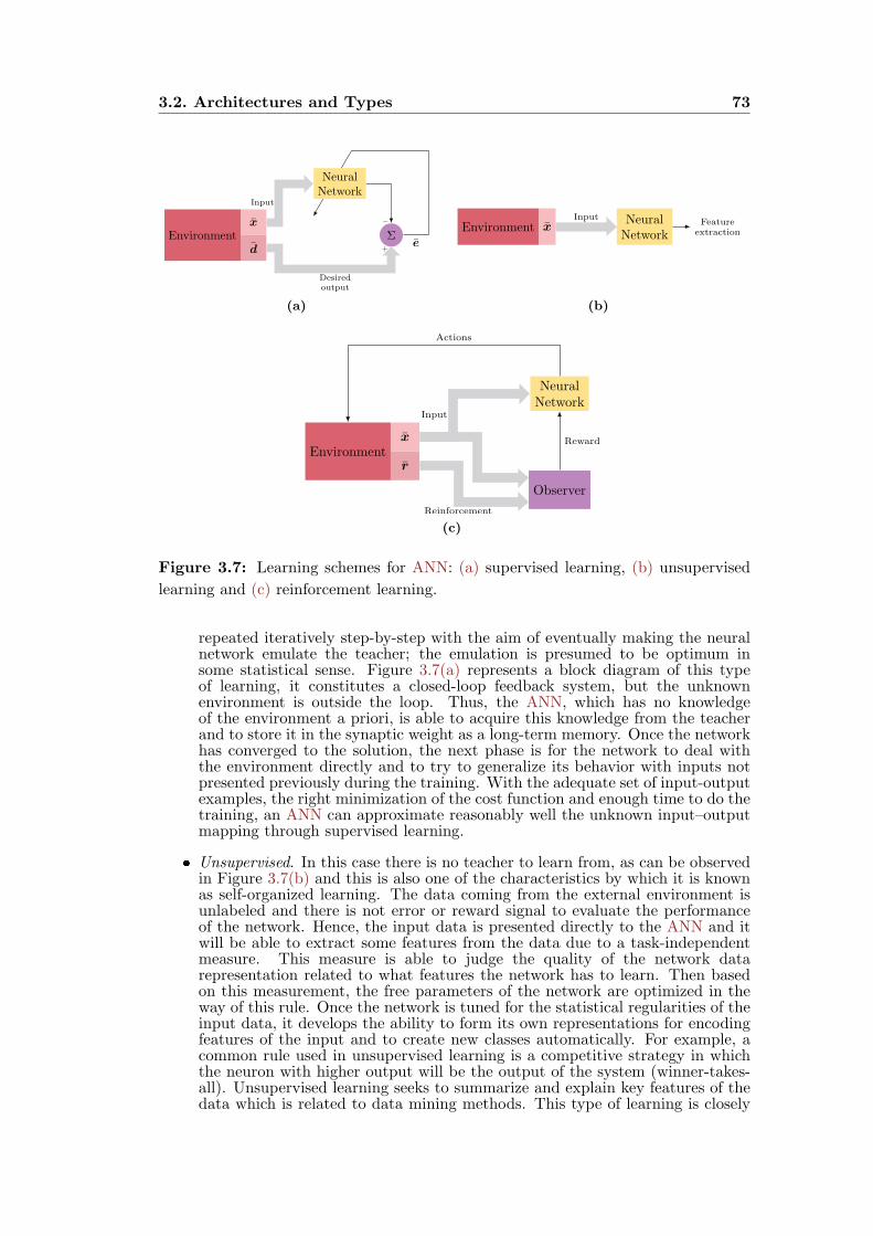
3.2. Architectures and Types 73
Environment
x
d
Neural
Network
Σ
Input
Desired
output
+
−
e
Neural
Network
(a)
Environment xNeural
Network
InputFeature
extraction
(b)
Environment
x
r
Neural
Network
Observer
Input
Reinforcement
Reward
Actions
(c)
Figure 3.7: Learning schemes for ANN: (a) supervised learning, (b) unsupervised
learning and (c) reinforcement learning.
repeated iteratively step-by-step with the aim of eventually making the neuralnetwork emulate the teacher; the emulation is presumed to be optimum insome statistical sense. Figure 3.7(a) represents a block diagram of this typeof learning, it constitutes a closed-loop feedback system, but the unknownenvironment is outside the loop. Thus, the ANN, which has no knowledgeof the environment a priori, is able to acquire this knowledge from the teacherand to store it in the synaptic weight as a long-term memory. Once the networkhas converged to the solution, the next phase is for the network to deal withthe environment directly and to try to generalize its behavior with inputs notpresented previously during the training. With the adequate set of input-outputexamples, the right minimization of the cost function and enough time to do thetraining, an ANN can approximate reasonably well the unknown input–outputmapping through supervised learning.
Unsupervised. In this case there is no teacher to learn from, as can be observedin Figure 3.7(b) and this is also one of the characteristics by which it is knownas self-organized learning. The data coming from the external environment isunlabeled and there is not error or reward signal to evaluate the performanceof the network. Hence, the input data is presented directly to the ANN and itwill be able to extract some features from the data due to a task-independentmeasure. This measure is able to judge the quality of the network datarepresentation related to what features the network has to learn. Then basedon this measurement, the free parameters of the network are optimized in theway of this rule. Once the network is tuned for the statistical regularities of theinput data, it develops the ability to form its own representations for encodingfeatures of the input and to create new classes automatically. For example, acommon rule used in unsupervised learning is a competitive strategy in whichthe neuron with higher output will be the output of the system (winner-takes-all). Unsupervised learning seeks to summarize and explain key features of thedata which is related to data mining methods. This type of learning is closely
74 3. Neural Networks
related to the feature extraction from the data, trying to group them such as inclustering or in Blind Source Separation (BSS). One of the common rules is themethods of moments, which consists of estimating the free parameters of thenetwork based on the moments of one or more random variables. Thus, theseunknown parameters can be estimated given the moments.
Reinforcement. This type of learning is more similar to the unsupervisedlearning, but the input-output mapping is done through the continuousinteraction of the ANN with the environment. In this case, there is not anerror signal and the desired output is not specified, but the network receivesa performance index to minimize. This index only indicates to the networkhow well or badly its performance is with respect to the reinforcement signalfrom the environment. Figure 3.7(c) presents an example of reinforcementlearning system, where a closed-loop feedback system is formed by an objectiveobserver which receives two signals from the environment: the input (x) andthe reinforcement (r) signals. Then, the objective observer elaborates a rewardsignal that indicates how well was the performance of the network to the lastinput and will be used to feed the network with the actual x. The networkoutput will serve as influencing actions in the environment that will changeit. In this process, the reinforcement signal arrives to the ANN one stepafter (delayed reinforcement), which eventually results in the generation ofthe heuristic reinforcement signal. The objective of this type of learning is tominimize a cost-to-go function, defined as a cumulative cost of actions over a setof steps rather than the immediate cost. Therefore, the network can find goodsolutions in the overall system behavior in order to discover these actions andfeed them back to the environment. However, the delayed reinforcement learningpresents two difficulties, i) the absence of desired outputs and ii) the delay onthe reward signal makes the ANN to solve a temporal credit assignment problem.In spite of these difficulties, reinforcement learning is appealing because it givessome mechanisms to learn a task interacting with the environment.
Hybrid. This type of learning consists of merging the previous types of learningin the same ANN. Thus, this type of learning could be applied in differentlayers of the same network or in different parts of a neural system with morethan one neural network. The idea of this type of learning is combining thebenefits of all of them and try to learn more complex tasks to solve faster theproblem. However, it is difficult to apply because of the different variables tominimize their cost and the various optimization functions that modify the freeparameters of the network. Yet, it is a powerful tool to learn multiple tasks ina given environment.
In Table 3.2, there is a classification of some of the most famous ANN models andlearning algorithms. The classification has been done attending to the morphology ofthe models and the way of training the free parameters. The more important modelsincluded in Table 3.2 are described as follows:
Simple perceptron. This architecture represents a binary classifier that candecide if a determined input corresponds to one class or another. It is a type oflinear classifier that makes its classifications based on the linear prediction ofa function combining wij with the feature vector. Rosenblatt (1958) describesthe perceptron as a neuron theory and also as a neural network.
Multilayer perceptron. This is a variant of the simple perceptron to whichhidden layers have been added, so that it is able to solve problems that are notlinearly separable. It was enunciated in Rosenblatt (1961), however there wasnot a learning algorithm able to train this type of networks until the arrival ofthe backpropagation algorithm.
ADAptative LINear Elements (ADALINE). It is a similar model ofneuron as the perceptron and it has a linear response whose inputs are normallycontinuous. The network uses memistors, which are resistors with memory able

3.2. Architectures and Types 75
ANN models & learning algorithms
Supervised Unsupervised
Feedforward Feedback Feedforward Feedback
Perceptron BSB LAM/OLAM ART
Adaline/Madeline Fuzzy Cog. Map Self-organizing map Hopfield
Multilayer Perceptron DTRNN/CTRNN Neocognitron BAM
Back Propagation BP through time PCA Network Elman
Time-delay NN Echo state Net
Cascade Correlation
Boltzman Machine
Support Vector Machine
LVQ
GRNN
CMAC
Reinforcement Hybrid
Q-Learning Radial basis function
Temporal difference methods Convolutional Networks
Table 3.2: Models of Artificial Neural Network and learning algorithms.
to perform logic operations and store information. It consists of a weight, a biasand a summation function, but the main difference with the perceptron is thatin the learning phase the weights are adjusted according to the weighted sumof the inputs (Widrow and Hoff, 1960). There is also a version with multipleADALINEs called MADALINE.
Hopfield. It is a type of RNN developed in Hopfield (1982), which serves as acontent-addressable memory with binary threshold nodes. Inside the network,the input data is compared against each node of the network, then one of theneurons will fire and it will be the output of the network for that input. Duringthe training this type of network guarantees the convergence to a local minimum,but this minimum can correspond to another pattern different from the one thatthe network has to learn. In addition, Hopfield proposed a way to understandthe human memory (Hopfield, 1982).
Boltzman machine. The Boltzman machine is another RNN with symmetricconnections whose neurons make stochastic decisions about whether to be on oroff (Hinton and Sejnowski, 1983). This type of network tries to extract featuresthat represent complex regularities in the training data. The learning algorithmused is very simple but it is too slow when networks are too dense. They aregenerally used as feature detectors in classification problems. In this type ofproblems they represent a cost function in which the neuron with the highestactivation would be the output of the network. It can be used also to reproducea set of input vectors with high probability in learning problems (Hinton andSejnowski, 1983).
Self-Organizing Map (SOM). It is also known as Kohonen network and itis a type of unsupervised learning neural network. The neurons are distributedregularly in the form of a grid, in general of two dimensions, whose purpose is tofind the structure of the data inserted in the network. So, it makes a dimensionalprojection from the set of data given to the neural space. During the training,
76 3. Neural Networks
the data vectors are the input to each neuron and they are compared with thecharacteristic weight vector of each neuron. Then, the neuron with the lowestdifference between its weight vector and the data vector is the winner andthis neuron together with the surrounding neurons modify their weight vector.Thus, the neurons which are together in the SOM are more similar than theones that are further away. SOMs also possess spatial information encoded intheir structure forming an ordered mapping. They were applied in visualizationapplications, and applications related with associative memory such as patternclassification (Kohonen, 1977).
Adaptive Resonance Theory (ART). It is a model of ANN whose operationis based on the way in which the human brain processes information. The modelconsists basically of two layers, one of inputs to sense the environment and oneof outputs, in which neurons compete with each other so that one is the responsewhich inhibits the rest. There is a feedback between the output layer and theinput one, so when an input is presented to the network if one of the outputresonates with it, then it is associated with the neuron. The center of thecluster will be moved to this class for a better adaptation to the next inputwith the feedback between layers. In case that any neuron output is activated,the network could be saturated or a new class could be added to resonate withit. This type of network was invented to solve the problem of stability andplasticity during the learning phase (Grossberg, 1987). There are also differentversions of the network.
Radial Basis Function (RBF). This type of networks consists normally ofthree layers: one input layer, a hidden layer with RBF and an output layer.A RBF is a function whose value depends on the distance from a point c,called center (Buhman, 2003). For example, one function normally used isthe Gaussian function that perfectly meets this property. Hence, the idea of theRBF network is to use the RBF layer as a separation layer in which the differentneurons behave as kernels, classifying the data and indicating to which neuronis closer. In addition, as RBFs are used to classify complex patterns, the hiddenlayer possesses more neurons than the input layer because a complex patternrecognition problem is more likely to be linearly separable in a high-dimensionalnonlinear space.
Support Vector Machine (SVM). This is not really a type of network butrather a type of algorithm used for training them. It is used along RBFs ormultilayer perceptrons with a single hidden layer. This type of algorithms areused to build networks to analyze data and solve problems related with therecognition of patterns, classification and regression analysis. SVM is usedto build a hyperplane that serves as decision surface that will be maximizedfollowing the separation margin between examples. Therefore, the SVM canmap new examples using the same space and predicted to which category theybelong, depending on the side of the gap they fall on. As RBFs, SVMs usehigh-dimensional nonlinear space to separate the data through a non-linearclassification (Cortes and Vapnik, 1995).
These are some of the most important architectures, also listed in Section 3.1.There exist many types of ANNs because there is not a unique established criterionto follow in order to build them. The idea is that a variety of ANNs can be builtdepending on various factors: number of neurons, number of layers, connectionsamong them (neurons and layers), etc. Also, the function that develops the neuronscan be configured using different activation functions or propagation rules. Inaddition, a more complex system can be built trying to gather together the operationof different ANNs. Thus, the idea is that each ANN solves part of a complexproblem by dividing it in simpler different subtasks. Apart from reducing the modelcomplexity, this modular approach will give other benefits such as simpler neuralmodels, scalability, robustness and computational efficiency among others (Buhman,1998).
3.3. Recurrent Neural Network 77
There is nothing preset and any architecture can be built from the fundamentalunit, the neuron, to the connections between them (neurons, layers or networks)and the form in which is trained. However, the application has to be present in thedesign of the architecture because there are some types of configurations that are moresuitable for an application than others. Based on the application, a RNN architecturehas been chosen in this Thesis because of its intrinsic properties and the ability tosimulate a dynamical behavior. Section 3.3 will explain in further detail the RNNarchitecture used in this Thesis and the properties for which these architectures areso interesting.
3.3 Recurrent Neural Network
This type of ANN deserves special attention due to the properties that are providedby the feedback loops inside the network. The feedback in the network could belocal, to the neuron itself or its surroundings, or global, to other layers or even otherneural networks giving more connectivity options. Thus, the presence of loops makespossible that the information about the activation status of the neurons flows insidethe network adding the property of short time memory to them. This representationis closer to biological neural networks in which recurrence is present in all parts ofthe nervous system. Adding short term memory to neural models makes a RNNable to do temporal processing and learn sequences, such as performing sequencerecognition/reproduction or temporal association/prediction. On the other hand,it will increase the complexity of the network and there exist some theoretical andpractical difficulties to implement in some applications so far.
The time variable is essential in the development of some tasks, such as vision,speech, signal processing, etc. Time representation could be done in a continuousor discrete way depending on the application. Including time in the performance ofan ANN makes possible to follow statistical variations in non stationary processes,such as speech signal, the market stock or the electric demand of a country. So, theaddition of this new variable makes possible to emulate the dynamics of a system.There are two forms of adding the temporal information to the neural architectures:i) implicitly, the network structure presents delays between synaptic connections, orii) explicitly, the external information is sampled and different samples are passedto the network so the temporal information is in the input (Haykin, 2009). Thislast type was commonly used with static feedforward ANNs before the feasibilityof implementing dynamic RNNs. Hence, the input has delayed samples of itself tointroduce temporal information which will be stored in the synaptic connections ofthe neural network.
Thus, it is necessary that memory would be added for an ANN to be dynamic.Long term memory is built in the network through the learning process after whichthe synaptic weights store all the data information used during the training. Onthe other hand, short term memory is required in case the problem to solve has atemporal dimension. One way of building this is the inclusion of feedback loops insidethe structure of the network, through time delays in the synaptic connections. Theinclusion of time delays is motivated by the biological functioning of the brain and isrelated on how the information is processed in the brain (Braitenberg, 1986).
The dynamics of RNNs has been widely studied since the 70s (Wilson andCowan, 1972). A dynamical environment which is constantly changing surroundseverything in daily life, so it is necessary to include dynamical properties in theartificial neural models to adapt them to the environment. RNNs can exhibit threedifferent dynamical behaviors: i) convergent, ii) oscillatory and iii) chaotic, dependingon the number of neurons and connections between them (Pasemann et al., 2003).However, these behaviors are not unique of RNNs, for example feedforward networkspresent convergence dynamics because of the characteristics of the applications inwhich they are used, such as content addressable memories or pattern recognition.On the other hand, oscillatory and chaotic dynamics only appear on RNNs, becauseof their neurons feedback (Dauce et al., 1998).
78 3. Neural Networks
The interest in the oscillatory and chaotic behavior has been the subject of manystudies in chemical, physical and biological systems (Tu, 2006; Goldbeter, 1997; Chay,1981). The appeal of RNNs is centered in their dynamic characteristics. Althoughhaving the same characteristics that feedforward networks, RNNs are more complexand there is not a clear way to train them in spite of several learning algorithms.However, a RNN has the ability not only to be mathematically a dynamic system byitself, but also to approximate arbitrary dynamic systems with an arbitrary precision(Pearlmutter, 1995). To do that, it is necessary to train adequately the networkin order to react and behave as such function according to the appropriate externalstimuli. The most widely used learning algorithms to train RNNs are gradient descentalgorithms, which correspond to the type of supervised learning (see Section 3.5).Furthermore, it is also possible for a RNN to learn the trajectory that describesthe dynamic behavior of a system such as in Pearlmutter (1989). In this case, thenetwork does not have any input and the connections are modified in order to followthe different states of the dynamic system.
Nevertheless, it is necessary to be careful with the addition of feedback to an ANN,because when applied improperly, they can produce harmful effects. The problemis that the application of feedback can cause a system a priori stable to becomeunstable. Therefore, it is also important to study the RNN stability to guarantee thatthe network is going to perform the task properly (see Section 3.3.1). The stabilityof a nonlinear dynamic system affects the whole system and implies some form ofcoordination between the individual parts of a system (Haykin, 2009). The stabilitystudy of a dynamical system makes possible to find solutions that avoid regions ofinstability and converge to a solution to the problem at hand.
Besides the approximation of arbitrary functions, RNNs are able to perform othertasks, such as content addressable memory, autoassociation, dynamic reconstructionof a chaotic process, etc. They are also able to map input sequences to outputsequences, with or without a teacher. One of the reasons to use them is thatRNNs are computationally more powerful and biologically more plausible than otheradaptive approaches such as Hidden Markov Models (no continuous internal states),feedforward networks and SVMs (no internal states at all). The global feedbackis a facilitator of the computational intelligence (Haykin, 2009). Thus, the networkincreases its capabilities to adapt to changes during the development of the applicationfor which it was built in the first place. Typically, RNNs were applied to many areassuch as control theory, robotics, pattern recognition, etc. But one area in whichthey are being used extensively is the time series forecasting due to its nonlineardynamics. In addition, RNNs are preferably used rather than time series analysisbecause they make accurate predictions, are computationally faster, make iterativeforecasts and deal with nonlinearity and non stationary input processes. Specifically,RNNs have found their place in predicting time series as Nonlinear AutoregressiveMoving Average with eXogenous inputs (NARMAX) prediction models (Mandic andChambers, 2001).
There exist different architectures also for RNNs depending on the loops ofthe network. Hopfield networks have been described in Section 3.2, other famousarchitectures are:
Fully recurrent network. All the neurons are connected with each other, thereexist connections from each neuron to the rest and itself. So there is not astructure defined as such, only a few neurons serve as inputs and outputs andthe rest will be hidden neurons. This structure has a high configuration capacity,however it is also a problem to train the network when there is a large amountof neurons. The reason is that the number of parameters to train increasesdrastically with the addition of more neurons. Such networks fit well when theapplication is not enough defined or it is necessary to use brute force to solvethe problem (Williams and Zipser, 1989).
Recurrent multilayer perceptron. This type of networks consists of more thanone layer which has feedback loops in the neurons of the same layer but thereis not any recurrence with previous or posterior layers. Hence, the network hasan input layer, one or more hidden layers and an output layer. The connection
3.3. Recurrent Neural Network 79
between them is done in a feedforward way. This type of network possesses theproperties of the multilayer perceptrons plus the ability to incorporate temporalbehavior through the feedback loops (Haykin, 2009).
Long Short Term Memory (LSTM) network. This type of network wasdeveloped in Hochreiter and Schmidhuber (1997) to solve the problem found inthe training of the layered networks. The network consists of an ANN to whichsome LSTM blocks have been added. A LSTM block consists of a processingunit that can remember a value for an arbitrary length of time, deciding whenthe input has to be remembered, when it should continue remembering it orforget the value, and when it should output the value. The property of storingan arbitrary value makes possible to work with long delays, and handle signalswith a mix of low and high frequency components. This network outperformsin tasks related with classification, processing and predicting time series withlags of data of unknown size.
Echo State Network (ESN). In this case the ESN is a specific type of RNNs thatpossesses a particular form, it has an input and output layers and between thema large reservoir of hidden units sparsely connected (typically 1% connectivity).The connection and number of neurons in the hidden reservoir are assignedrandomly and the only weights that need to be trained are the ones in theoutput layer. Thus, this neural network is appropriate at reproducing specifictemporal patterns because of its nonlinearity properties (Jaeger, 2001).
Elman and Jordan networks. This type of network follows a similar conceptthan the Hopfield networks. The idea consists of three layers (input, hiddenand output) plus a context layer that stored the state of the hidden layer fromthe previous time step. The context units are connected only to the hiddenlayer, maintaining a copy of the previous values of the hidden units beforethe learning rule is applied. Thus, the network maintains a state, being able toperform tasks related with prediction better than feedforward networks (Elman,1990). Jordan networks are similar to Elman ones, but with the peculiarity thatthe context units take their input from the output layer rather than the hiddenlayer (Jordan, 1986).
Some special architectures have been introduced above and only referred to somepeculiarities related with their structure. However, there exist other architecturesbased on differential equations in order to model the neural behavior to externalstimuli. These types of RNNs try to use the dynamical system theory to modelbiological neural networks that include the time as reference and feedback loops aspart of the network structure, such as in the brain. There exist two different typesof networks depending on the time basis used: i) discrete or ii) continuous. DiscreteTime RNN (DTRNN) uses a difference equation to describe the neural model. Theidea is that each time step the neuron activation evolves to a new value depending onthe previous one (Pasemann, 1993). The mathematical representation of the DTRNNis shown in Equation 3.6.
yi[k + 1] = fi(xi[k], y1[k], . . . , yn[k]) = σ
n∑j=1
wij · yj [k] + xi[k] + θi
(3.6)
where, yi is the output of the ith neuron, σ(·) is the activation function, wij is theneural weight that connects the ith neuron with jth neuron, xi is the input value ofthe ith neuron and θi is its bias value.
Equation 3.6 may be represented as an alternative vector form as:
y[k + 1] = fα(x[k],y[k]) = φ (W · y[k] + x[k] + θ) (3.7)
where, y is the output vector of the neurons, W is the matrix of the synaptic weights,x is the input vector and θ is the bias vector.
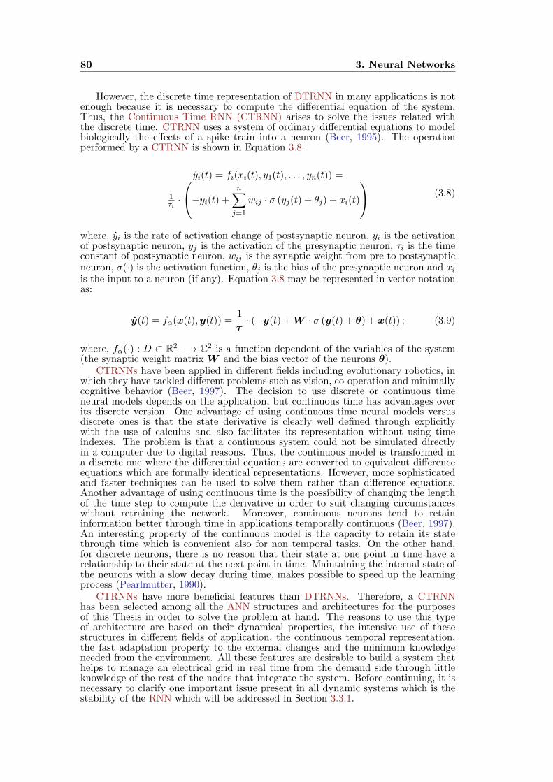
80 3. Neural Networks
However, the discrete time representation of DTRNN in many applications is notenough because it is necessary to compute the differential equation of the system.Thus, the Continuous Time RNN (CTRNN) arises to solve the issues related withthe discrete time. CTRNN uses a system of ordinary differential equations to modelbiologically the effects of a spike train into a neuron (Beer, 1995). The operationperformed by a CTRNN is shown in Equation 3.8.
yi(t) = fi(xi(t), y1(t), . . . , yn(t)) =
1τi·
−yi(t) + n∑j=1
wij · σ (yj(t) + θj) + xi(t)
(3.8)
where, yi is the rate of activation change of postsynaptic neuron, yi is the activationof postsynaptic neuron, yj is the activation of the presynaptic neuron, τi is the timeconstant of postsynaptic neuron, wij is the synaptic weight from pre to postsynapticneuron, σ(·) is the activation function, θj is the bias of the presynaptic neuron and xiis the input to a neuron (if any). Equation 3.8 may be represented in vector notationas:
y(t) = fα(x(t),y(t)) =1
τ· (−y(t) +W · σ (y(t) + θ) + x(t)) ; (3.9)
where, fα(·) : D ⊂ R2 −→ C2 is a function dependent of the variables of the system(the synaptic weight matrix W and the bias vector of the neurons θ).
CTRNNs have been applied in different fields including evolutionary robotics, inwhich they have tackled different problems such as vision, co-operation and minimallycognitive behavior (Beer, 1997). The decision to use discrete or continuous timeneural models depends on the application, but continuous time has advantages overits discrete version. One advantage of using continuous time neural models versusdiscrete ones is that the state derivative is clearly well defined through explicitlywith the use of calculus and also facilitates its representation without using timeindexes. The problem is that a continuous system could not be simulated directlyin a computer due to digital reasons. Thus, the continuous model is transformed ina discrete one where the differential equations are converted to equivalent differenceequations which are formally identical representations. However, more sophisticatedand faster techniques can be used to solve them rather than difference equations.Another advantage of using continuous time is the possibility of changing the lengthof the time step to compute the derivative in order to suit changing circumstanceswithout retraining the network. Moreover, continuous neurons tend to retaininformation better through time in applications temporally continuous (Beer, 1997).An interesting property of the continuous model is the capacity to retain its statethrough time which is convenient also for non temporal tasks. On the other hand,for discrete neurons, there is no reason that their state at one point in time have arelationship to their state at the next point in time. Maintaining the internal state ofthe neurons with a slow decay during time, makes possible to speed up the learningprocess (Pearlmutter, 1990).
CTRNNs have more beneficial features than DTRNNs. Therefore, a CTRNNhas been selected among all the ANN structures and architectures for the purposesof this Thesis in order to solve the problem at hand. The reasons to use this typeof architecture are based on their dynamical properties, the intensive use of thesestructures in different fields of application, the continuous temporal representation,the fast adaptation property to the external changes and the minimum knowledgeneeded from the environment. All these features are desirable to build a system thathelps to manage an electrical grid in real time from the demand side through littleknowledge of the rest of the nodes that integrate the system. Before continuing, it isnecessary to clarify one important issue present in all dynamic systems which is thestability of the RNN which will be addressed in Section 3.3.1.

3.3. Recurrent Neural Network 81
3.3.1 Stability
Stability is a property of dynamic systems to study the solutions of the differentialequations and their trajectories, remaining inside or in the neighborhood of a setof points called orbit. There are different stability criteria to address this propertyfor a system. For example, the Bounded Input Bounded Output (BIBO) stabilitycriterion is normally used to refer to the stability of the input and output of asystem. According to this criterion, the stability of a system depends on the growthof the output, which is bounded due to bounded input, initial condition or unwanteddisturbance. In general, RNNs are systems that meet the BIBO stability criterion.This criterion is within the structure of the RNNs as they are built with activationfunctions that present saturation nonlinearities and limit the growth of the output.Thus, this stability criterion does not provide any relevant information to the stabilityof a RNN. Normally, the stability criterion of nonlinear dynamic systems is relatedwith the Lyapunov stability theory (Lyapunov, 1992).
Before describing the Lyapunov theory, it is necessary to understand someconcepts. A dynamic system is a system whose state varies with time and differentmodels can be used to do it. Usually, dynamic systems are represented by a state-space models which consist of a set of state variables whose values possess enoughinformation to predict the temporal evolution of the system (Haykin, 2009). Themathematical expression of this model is described in Equation 3.10.
d
dtx(t) = F (x(t)) (3.10)
where, x(t) = [x1(t), x2(t), . . . , xN (t)]T is the state vector containing the N differentstates in which the system is divided and F (·) is the nonlinear function evaluated foreach state of the system. N is the system order. The function F (·) could dependexplicitly on time, autonomous, or not, non autonomous.
Equation 3.10 could be adapted to represent the RNN activations so the dynamicsystem theory can be applied to them. The state space representation is useful becauseit provides a visual and conceptual tool to analyze the dynamics of a system ratherthan numeric solutions of the system. So, the system has been divided in N statesthat evolve during time. These changes in time can be represented as a curve in thestate space, and it is called trajectory or orbit of the system. Equation 3.10 describesthe motion of a point in an N -dimensional space, whose solutions are represented intrajectories and the tangent vector of each point represents the velocity at the initialcondition. For each possible state, there will be a tangent vector and the assembly ofthe tangent vectors is described as a vector field. Then, the vector function F (x(t))can be seen as a velocity vector field, or a vector field. The trajectories for differentinitial conditions can be grouped in the system state portrait, which includes all thesystem points in which the system is defined and possesses information about the flowof the dynamic system (Guckenheimer and Holmes, 1983).
The solution uniqueness have to be also guaranteed for the state space equationonly under certain conditions, which restricts the form of F (x(t)). A solution tothe system exists if F (x(t)) is continuous in all its arguments but it is necessary tomeet the Lipschitz condition for uniqueness (Haykin, 2009). Once the solutions toEquation 3.10 are found, the stability of those solutions can be analyzed based onthe equilibrium of the states. To begin with the stability study of the states, it isnecessary to define when a state is at equilibrium.
Let x∗ ∈ D be an equilibrium state of the system, such that F (x∗) = 0. Normally,the equilibrium state is also named singular point because the trajectory can betransformed into a point itself. At the equilibrium state, dx(t)/dt → 0 and thereforea possible solution to the system is the constant function x(t) = x∗. Because ofthe uniqueness of solution, no other curve will pass through x∗. Thus, to studythe stability of a system such as Equation 3.10, it is necessary to analyze thebehavior of the orbits near to an equilibrium state (Kuznetsov, 1998). The nonlinearfunction F (x(t)) is considered to be smooth enough in order to be linearized in theneighborhood of x∗. If the vector function F (·) is a C1 vector field (the first derivative
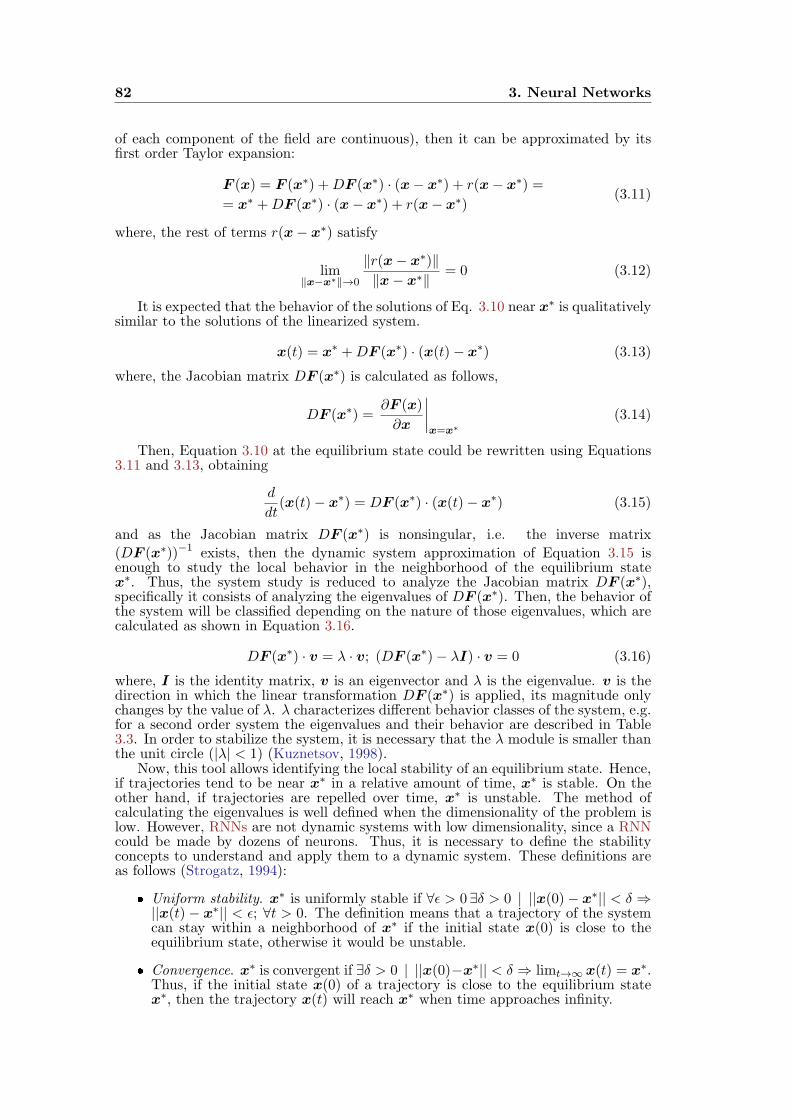
82 3. Neural Networks
of each component of the field are continuous), then it can be approximated by itsfirst order Taylor expansion:
F (x) = F (x∗) +DF (x∗) · (x− x∗) + r(x− x∗) =
= x∗ +DF (x∗) · (x− x∗) + r(x− x∗)(3.11)
where, the rest of terms r(x− x∗) satisfy
lim∥x−x∗∥→0
∥r(x− x∗)∥∥x− x∗∥
= 0 (3.12)
It is expected that the behavior of the solutions of Eq. 3.10 near x∗ is qualitativelysimilar to the solutions of the linearized system.
x(t) = x∗ +DF (x∗) · (x(t)− x∗) (3.13)
where, the Jacobian matrix DF (x∗) is calculated as follows,
DF (x∗) =∂F (x)
∂x
∣∣∣∣x=x∗
(3.14)
Then, Equation 3.10 at the equilibrium state could be rewritten using Equations3.11 and 3.13, obtaining
d
dt(x(t)− x∗) = DF (x∗) · (x(t)− x∗) (3.15)
and as the Jacobian matrix DF (x∗) is nonsingular, i.e. the inverse matrix
(DF (x∗))−1 exists, then the dynamic system approximation of Equation 3.15 isenough to study the local behavior in the neighborhood of the equilibrium statex∗. Thus, the system study is reduced to analyze the Jacobian matrix DF (x∗),specifically it consists of analyzing the eigenvalues of DF (x∗). Then, the behavior ofthe system will be classified depending on the nature of those eigenvalues, which arecalculated as shown in Equation 3.16.
DF (x∗) · v = λ · v; (DF (x∗)− λI) · v = 0 (3.16)
where, I is the identity matrix, v is an eigenvector and λ is the eigenvalue. v is thedirection in which the linear transformation DF (x∗) is applied, its magnitude onlychanges by the value of λ. λ characterizes different behavior classes of the system, e.g.for a second order system the eigenvalues and their behavior are described in Table3.3. In order to stabilize the system, it is necessary that the λ module is smaller thanthe unit circle (|λ| < 1) (Kuznetsov, 1998).
Now, this tool allows identifying the local stability of an equilibrium state. Hence,if trajectories tend to be near x∗ in a relative amount of time, x∗ is stable. On theother hand, if trajectories are repelled over time, x∗ is unstable. The method ofcalculating the eigenvalues is well defined when the dimensionality of the problem islow. However, RNNs are not dynamic systems with low dimensionality, since a RNNcould be made by dozens of neurons. Thus, it is necessary to define the stabilityconcepts to understand and apply them to a dynamic system. These definitions areas follows (Strogatz, 1994):
Uniform stability. x∗ is uniformly stable if ∀ϵ > 0∃δ > 0 | ||x(0)− x∗|| < δ ⇒||x(t)− x∗|| < ϵ; ∀t > 0. The definition means that a trajectory of the systemcan stay within a neighborhood of x∗ if the initial state x(0) is close to theequilibrium state, otherwise it would be unstable.
Convergence. x∗ is convergent if ∃δ > 0 | ||x(0)−x∗|| < δ ⇒ limt→∞ x(t) = x∗.Thus, if the initial state x(0) of a trajectory is close to the equilibrium statex∗, then the trajectory x(t) will reach x∗ when time approaches infinity.
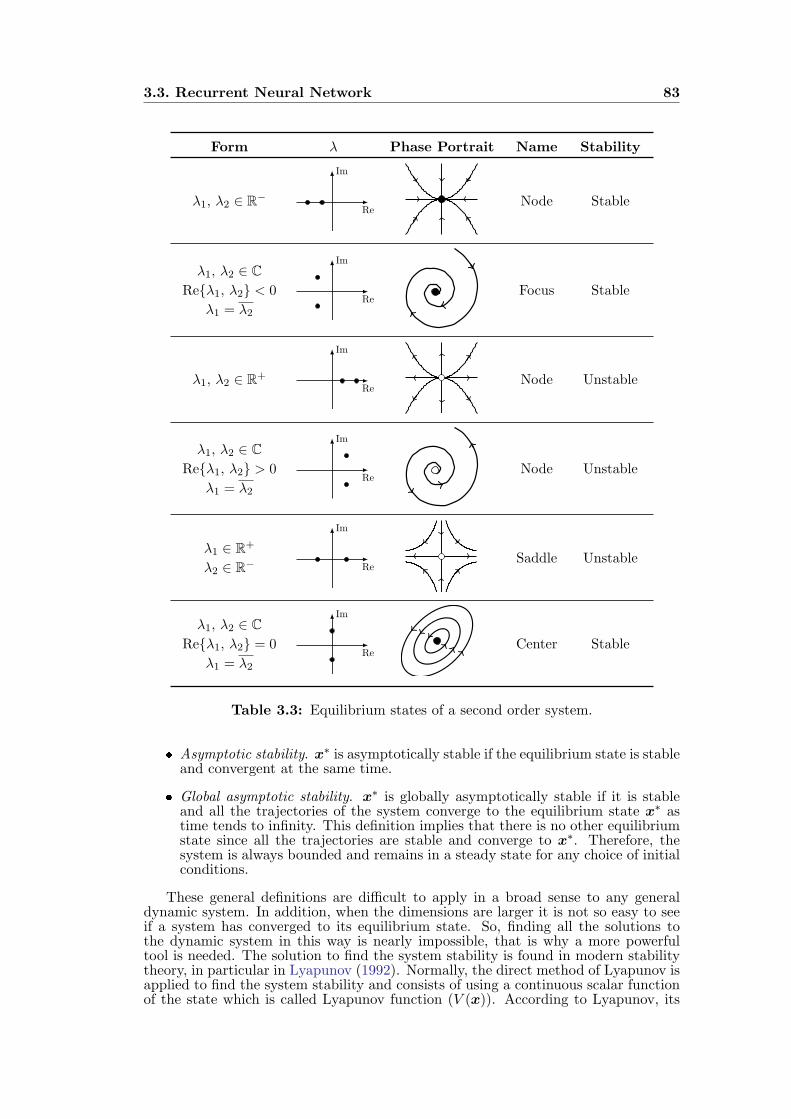
3.3. Recurrent Neural Network 83
Form λ Phase Portrait Name Stability
λ1, λ2 ∈ R−Re
Im
Node Stable
λ1, λ2 ∈ CReλ1, λ2 < 0
λ1 = λ2
Re
Im
Focus Stable
λ1, λ2 ∈ R+Re
Im
Node Unstable
λ1, λ2 ∈ CReλ1, λ2 > 0
λ1 = λ2
Re
Im
Node Unstable
λ1 ∈ R+
λ2 ∈ R− Re
Im
Saddle Unstable
λ1, λ2 ∈ CReλ1, λ2 = 0
λ1 = λ2
Re
Im
Center Stable
Table 3.3: Equilibrium states of a second order system.
Asymptotic stability. x∗ is asymptotically stable if the equilibrium state is stableand convergent at the same time.
Global asymptotic stability. x∗ is globally asymptotically stable if it is stableand all the trajectories of the system converge to the equilibrium state x∗ astime tends to infinity. This definition implies that there is no other equilibriumstate since all the trajectories are stable and converge to x∗. Therefore, thesystem is always bounded and remains in a steady state for any choice of initialconditions.
These general definitions are difficult to apply in a broad sense to any generaldynamic system. In addition, when the dimensions are larger it is not so easy to seeif a system has converged to its equilibrium state. So, finding all the solutions tothe dynamic system in this way is nearly impossible, that is why a more powerfultool is needed. The solution to find the system stability is found in modern stabilitytheory, in particular in Lyapunov (1992). Normally, the direct method of Lyapunov isapplied to find the system stability and consists of using a continuous scalar functionof the state which is called Lyapunov function (V (x)). According to Lyapunov, its
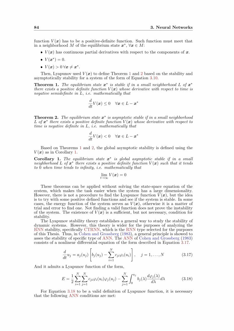
84 3. Neural Networks
function V (x) has to be a positive-definite function. Such function must meet thatin a neighborhood M of the equilibrium state x∗, ∀x ∈M :
V (x) has continuous partial derivatives with respect to the components of x.
V (x∗) = 0.
V (x) > 0 ∀x = x∗.
Then, Lyapunov used V (x) to define Theorem 1 and 2 based on the stability andasymptotically stability for a system of the form of Equation 3.10.
Theorem 1. The equilibrium state x∗ is stable if in a small neighborhood L of x∗
there exists a positive definite function V (x) whose derivative with respect to time isnegative semidefinite in L, i.e. mathematically that
d
dtV (x) ≤ 0 ∀x ∈ L− x∗
Theorem 2. The equilibrium state x∗ is asymptotic stable if in a small neighborhoodL of x∗ there exists a positive definite function V (x) whose derivative with respect totime is negative definite in L, i.e. mathematically that
d
dtV (x) < 0 ∀x ∈ L− x∗
Based on Theorems 1 and 2, the global asymptotic stability is defined using theV (x) as in Corollary 1.
Corollary 1. The equilibrium state x∗ is global asymptotic stable if in a smallneighborhood L of x∗ there exists a positive definite function V (x) such that it tendsto 0 when time tends to infinity, i.e. mathematically that
limt→∞
V (x) = 0
These theorems can be applied without solving the state-space equation of thesystem, which makes the task easier when the system has a large dimensionality.However, there is not a procedure to find the Lyapunov function V (x), but the ideais to try with some positive defined functions and see if the system is stable. In somecases, the energy function of the system serves as V (x), otherwise it is a matter oftrial and error to find one. Not finding a valid function does not prove the instabilityof the system. The existence of V (x) is a sufficient, but not necessary, condition forstability.
The Lyapunov stability theory establishes a general way to study the stability ofdynamic systems. However, this theory is wider for the purposes of analyzing theRNN stability, specifically CTRNN, which is the RNN type selected for the purposesof this Thesis. Thus, in Cohen and Grossberg (1983), a general principle is showed toasses the stability of specific type of ANN. The ANN of Cohen and Grossberg (1983)consists of a nonlinear differential equation of the form described in Equation 3.17.
d
dtuj = aj(uj)
[bj(uj)−
N∑i=1
cjiφi(ui)
], j = 1, . . . , N (3.17)
And it admits a Lyapunov function of the form,
E =1
2
N∑i=1
N∑j=1
cjiφi(ui)φj(uj)−N∑j=1
∫ uj
0bj(λ)
dφj(λ)
dλdλ (3.18)
For Equation 3.18 to be a valid definition of Lyapunov function, it is necessarythat the following ANN conditions are met:
3.4. Artificial Neural Network in action: Applications 85
The synaptic weights are symmetric, cij = cji.
The function aj(uj) is nonnegative, i.e. aj(uj) ≥ 0.
The nonlinear activation function φj(uj) satisfies the monotonicity condition,
i.e. φj(uj) =dφj(uj)
duj≥ 0.
Finally, the Cohen-Grossberg theorem could be stated as follows:
Theorem 3. Provided the system of nonlinear differential equations of Equation 3.17which satisfies the condition of symmetry, nonegativity and monotonicity, admits thedefinition of a Lyapunov function E of the form of Equation 3.18 that satisfies thecondition
dE
dt≤ 0
then the neural system of Equation 3.17 is Lyapunov stable in the sense of Theorem1.
Consequently, this theorem provides a powerful tool to build RNNs guaranteeingthat they are stable structures. And it is not necessary to solve the entire systemof differential equations, or search for a Lyapunov function that meets the stabilityconditions. In this Thesis, the Cohen-Grossberg theorem is used to build the neuralmodels of CTRNN, following its condition and assuring that the network is Lyapunovstable.
3.4 Artificial Neural Network in action: Applications
In the first part of this Chapter, the basics of ANNs and different structures commonlyused have been explained. The ANN application is present in all parts of its designboth its structure and its training. ANNs can be applied almost to any application,but with some considerations such as enough data to train the network or a feasiblestructure to be trained in enough time. In addition, ANNs cannot be used inapplications with not enough data because they do not have enough informationto extract features from it.
In spite of not being good for arithmetics and precise calculations, ANNs canextract patterns if there are enough data even with noise. They can always give ananswer to the input data even when the input is not complete and are well fittedin applications in which they can infer a function or relationship from observations.ANNs are particularly useful in applications where the function they infer from thedata is too complex and there are nonlinear relationships among them. But with allthese advantages comes a great disadvantage when the complexity of the problemrequires a large neural structure because any interpretation can be drawn from thedata. The main problem for large structures is the number of free parameters, suchas hidden nodes, synaptic weights, learning rates, etc.
At the same time, implementing an application with an ANN has the advantagesalready described in Section 3.1.1. Thus, when applying ANNs, it is necessary toconsider the pros and cons. Recently, an intensive use of ANNs has been done due tothe immense data available at any application and the increase power of computation.ANNs are beginning to expand into a variety of fields different from the classic AIones, such as financial, marketing, industrial or energy, among other fields of interest.In the application of ANNs, there are differences between candidate, developing andalready demonstrated applications. In other words, it is necessary to clarify the statusof development, implementation and validation of the ANN in each application. Acandidate application is an application that it could be solved potentially by an ANNbut for the moment there has not been a successful implementation. Developingapplications are those in which the problem has been deeply studied and there existsan ANN prototype that has been trained with a simplified version of the problem.Finally, demonstrated applications are the ones in which an ANN structure has
86 3. Neural Networks
already been used to solve a real problem. With respect to the use of ANNs over time,different categories of applications have been discovered, in which ANNs develop anexcellent job and are efficient solving problems in these areas. Those areas are asfollows (Jain et al., 1996; Basheer and Hajmeer, 2000; Haykin, 2009):
Classification. This is a classic AI problem consisting of identifying which presetcategories belong to a new incoming data. The classification is done based onthe previous data observations whose categories or classes are known. ANNsare used in this type of tasks due to their input-output mapping abilities.The classification is done normally through a supervised learning algorithmin which an input, represented by a feature vector, is shown to the networkand at the same time the class corresponding to the input is used to adjustthe free parameters of the network, obtaining the desired result. In addition,there is an unsupervised version of classification known as clustering, consistingof grouping data without any knowledge based on an internal metric and thesimilarities or dissimilarities between the input patterns. In any case, the ANNin charge of solving the task extracts the features from the data and obtainsan internal representation from them to be assigned to one of the classes. Thedata could be of different nature, e.g. continuous or discrete inputs, inputsfrom different sources such as different sensors, and the classification couldbe done in different ways: categories, ordinal, integer-valued or real-valued.Inside this field, there also exist problems related with pattern recognition,decision making or detection, since they consist of mapping inputs into thecorresponding outputs. Among the different applications, in which ANNshave been successfully applied in real classification problems, such as characterrecognition, speech recognition, EEG waveform classification, fault diagnosis,image classification, cancer detection, etc.
Data processing. Many applications can be found within this field, but allof them are related. All of these applications use a starting set of inputswhich are manipulated to obtain meaningful information. ANNs are used toinfer a relationship between the input and the output, extracting only thevalid information and processing it to solve the task assigned. Therefore, theapplication itself is the one that considers which information is meaningfuland which can be discarded. This scope also covers all applications involvingsignal processing which consists of treating or transferring the informationcontained within different physical, abstract or symbolic forms denominatedsignals. Thus, ANNs models manipulate the information of the signal to obtaindifferent goals, taking advantage of the learning and adaptivity abilities ofthem. For example, ANNs have been used in filtering tasks which consistof modifying the characteristics of the signal itself to obtain a new signal ofthe characteristics required by the system. Inside filtering tasks, ANN hasbeen used for tasks involving adaptive filtering such as noise reduction or echocancellation. In addition, ANNs have been used in: validation (ensuring thatthe data are correct and useful), compression (consisting of dimensionalityreduction), analysis (involved in the collection, organization, interpretation andpresentation of data), multiplexing information, image processing, encodinginformation to send it through a canal, speech processing, etc.
Function approximation. It is also known as model building and consists offinding the relationships that exist between the different data available, ifany. Suppose that a set of labeled observations of input-output data havebeen generated by an unknown function. Then, an ANN is used to estimatethe unknown function underlying rules relating the inputs to the outputs.Multilayer ANNs are considered universal approximators that can approximateany arbitrary function to any degree of accuracy (Cybenko, 1989). ANNs arealso used to compute regression in the data, which is a special case of functionapproximation. Function approximation with ANNs is applied typically totwo different problems: i) no explicit mathematical expression is available, i.e.the data are obtained from experiments or observations, and ii) substituting

3.4. Artificial Neural Network in action: Applications 87
theoretical models too complex to analyze where the data from the model areused directly. Related with this task, ANN structures are used to predicttime series. A time series is a sequence of successive points over a timeinterval. ANNs are used in time series forecasting to analyze the data inorder to extract meaningful statistics and other characteristics and then predicta future value based on the information extracted plus previously observedvalues. Forecasting is an important application very useful in decision-makingin business, science and engineering. For example, typical applications of timeseries forecasting with ANNs are: stock market prediction, weather forecasting,electricity demand forecasting, etc.
Optimization. This field of application is related with finding solutions toproblems in the most efficient way with the less resources possible. Specifically,optimization consists of finding a solution that maximizes or minimizes anobjective function that satisfies a set of constraints. A wide variety of problemsin mathematics, statistics, engineering, science, medicine and economics can beinterpreted as optimization problems. For example, well known optimizationproblems are the travel salesman problem or the NP-complete problem. ANNsare used in optimization because they are efficient solving complex and nonlinearoptimization problems. ANNs have also been used in fitness approximationwhich is a method consisting of reducing the evaluations of a fitness function toreach a target solution.
Association. This type of applications establishes a set of relationships betweenthe data, which allow identifying some patterns and reproduce them to a giveninput. Content-addressable memory is a type of association application whichconsists of a quick search for a given input to obtain the right output previouslystored. An advantage of this type of applications is that the content is accesseddirectly, so that the output will be retrieved correctly even though the inputpresents some degree of corruption or it is affected by noise. An ANN forassociation tasks is trained on noise-free data and then used to classify noisecorrupted data as in novelty detection. The network will also be used to corrector reconstruct the corrupted data or completely missing data. For example,Hopfield networks and multilayer perceptrons are used in this type of tasks.In addition, association problems are also related with establishing similaritiesbetween states that are close in time or space. Inspired in the characteristic ofthe brain to organize information, the SOMs are other ANN structures that solvetasks related with association. SOMs are spatial maps of the input patterns, inwhich the information contained in the input patterns are distributed spatiallyin the lattice that forms the neurons and the activation of each of them isindicative of intrinsic statistical features of the inputs.
Control. It is a discipline which applies control theory to make a systembehave in a wanted or desired way. For example, a dynamic model definedby u(t), y(t), where u(t) is the control input and y(t) is the resulting outputof the system at time t. The goal is to generate a control input u(t) such that thesystem follows a desired trajectory determined by a reference model. Examplesof these implementations are the speed control of a motor or fix the motor toa determined position. Thus, the idea is to design an ANN with the sensoryinput of the system and elaborate an output that the system will follow basedon system feedback. A neural controller is not an easy task to train but withthe adequate inputs and the right system design, a nonlinear controller could beused to fulfill the task that otherwise would be too complex. A field related withcontrol is robotics, in which robots are built using control, sensory feedback andinformation processing. ANNs are used to establish some nonlinear relationshipsbetween the sensory inputs of the robot and the desired response of the robot,e.g. manipulators, speech recognition, gestures and artificial emotions. Anothercontrol field in which ANNs are being applied is in the prosthesis, which consistsof replacing a missing body part with an artificial device. ANNs are used toprocess the information coming from the muscle around the missing body partand elaborate a response to move the prosthetic in the right way.
88 3. Neural Networks
In all these applications, the idea of processing information with ANN ispresent. They also take advantage of their characteristics: i) input-output mapping,ii) nonlinearity and iii) feature extraction. All the applications, involving thesecharacteristics can be solved by an ANN approximation. However, some neuralarchitectures are best suited to solve a certain type of problems, such as SOMs whichimplement content-addressable memory applications or RNNs which are best forprediction, time-series representation, adaptive filtering, control dynamics, etc. dueto the presence of feedback. In this Section, some applications were shown in whichANNs can be applied, but they can also be applied to: security (face identification,biometrics), data mining (or knowledge discovery in databases), medical diagnosis(cancer detection, processing medical images), financial applications (automatedtrading systems) or system identification (e-mail spam filtering).
There are many fields in which ANNs have been successfully applied but theirexpansion continues. A promising field of application for ANNs is the electricityfield because with the arrival of the Smart Grid (SG) is increasing the need forfast information processing and using their features for prediction and time seriesrepresentation would help with the management of the grid. As part of this Thesis,the electricity field is strongly presented so Section 3.4.1 reviewed how ANNs havebeen used in power systems.
3.4.1 Artificial Neural Network in Electrical Applications
With the advent of SG, algorithms are becoming increasingly necessary to help toautomate the continuous operation of the grid as its complexity is also increasing.Signal processing is becoming an essential tool to understand, plan, design and operatethe complex processes of the grid. Many electrical applications involve the use of signalprocessing as a tool to analyze them and the need of these techniques is becoming areal fact. The reasons are the vast amount of data available for correlation, diagnosisand analysis inside power systems nowadays (Ribeiro et al., 2014).
There exist several reasons why applying ANNs to power systems, such as theirlearning ability from the environment, fault tolerance, distributed system, real timeapplication, etc. They are also self-organized structures, which create their owndata representation during the learning process in real-time operation, since thecomputation can be done in parallel and the redundancy of the structure preventsthe degradation performance of the network in any fault case (Momoh, 2012). Inaddition, ANNs need fewer constraints than other algorithms when using them inpower system applications. The data used are straight forwardly handled withouta significant reduction or manipulation of the variables. Another advantage of suchalgorithms is that they add value to the investments made in infrastructure within theSG. The reason is that once trained for the task they are undertaking, ANNs can beintegrated into new ICT systems without assuming higher costs. Hence, such methodsof system performance evaluation are very much cost-effective and will not hinder theconsumer welfare by an unnecessary increase in electricity price (Sen et al., 2015).ANNs have been successfully applied in different applications related with powersystems: i) security assessment, ii) fault detection and diagnosis, iii) load forecasting,iv) transient stability, v) control analysis, vi) economic dispatch and vii) systemprotection and design (Haque and Kashtiban, 2007). Some of the most importantapplications are explained as follows:
Load forecasting. One of the main applications in which ANNs have beenapplied is load forecasting. The grid operation involves planning the differentgenerators to accomplish the real-time matching of the demand. In addition,load forecasting does not only serve for the system daily operation, but toprevent future failures or system congestion, ensuring that users always receivetheir electricity. Thus, load forecasting is related to financial, development,expansion and planning, and it is important to make accurate predictions forsystem enhancement. There exist three different forms to predict the griddemand based on the forecast time length: short-term, mid-term and long-termload forecast.
3.4. Artificial Neural Network in action: Applications 89
– Short-term load forecasting consists of elaborating a forecast using atemporal interval from an hour to a week which is important for dif-ferent applications such as real time control, economic dispatch, unitcommitment, etc. (Haque and Kashtiban, 2007). For example, Parket al. (1991) used a perceptron to make load forecasts in intervals ofhours and days by using the weather and load information. They showedbetter performance of load forecasting with ANNs than using conventionaltechniques. In Germond et al. (1993), a SOM was used to short-termforecasting of peak electrical loads by using the load data of a real system.In Hippert et al. (2001), there is a description of different ANN modelsused for short load forecasting. Different ANN structures have been used,such as multilayer perceptrons, SOM, RNN, RBF, etc., using differentinput data, like weather conditions, holidays, weekends and special sportmatches days inside the forecasting model. But typically, the data usedfor short term load forecasting are time factors and weather data. Inthese models different prediction horizons have been used such as 1 hour,24 hour (a day), 168 hour (a week) for predicting the entire demand curveor peak hours. ANNs in short-term load forecasting are known to solve thelimitations of other traditional models. They have overcome the difficultiesto find relationships between all variable attributes and instantaneous loaddemand in order to adapt rapidly to the nonlinear system-load changes.
– Mid-term load forecasting covers a prediction horizon time from weeks toa couple of years. The data normally used to elaborate the predictionsare different from the ones used to short-term load forecasting. Mid-termforecasting is sensitive to growth factors, which are factors that influencedemand such as seasonal variations, addition of new loads, maintenancerequirements of large consumers, etc. However, mid-term forecasting is notas accurate as short-term forecasting on power system operations. In Feilatand Bouzguenda (2011), a multilayer perceptron is used to forecast themonthly peak load based on the historical monthly load data, temperature,humidity and wind speed. Normally, the data used to elaborate theforecasts consist of historical load, weather, economics and demographicdata (Feilat and Bouzguenda, 2011). With this information, it is possibleto plan the maintenance of a certain plant during a time period, major testsin the system, commissioning events, determine outage times of plants, etc.Tsekouras et al. (2006) use an adaptive ANN, which properly transformsthe input variables to differences or relative differences, in order to predictenergy values not included in the training set. Another example of yearlymid-term load forecasting is described in Bunnoon (2011). An ANN isused to forecast a year ahead the grid demand based on different factors,such as temperature, humidity, wind speed, rainfall, industrial index andconsumer price index. It is used for a unit commitment and a fuel reserveplanning in the power system.
– Long-term load forecasting has the larger prediction horizon and covers atime span from a couple of years to decades. In this type of forecasting,quick changes in the demand are not as significant as in other horizonprediction. Grid operators need accurate forecasts that allow the powersystem to implement new strategies and continue its expansion. Long-term forecasting as mid-term forecasting uses growth factors to elaboratepredictions and take into account long historical data of the power systemand other macro economic variables related with power systems, such asdemographic growing, time factors, facilities investment or sales, regionaldevelopment, energy supply price, etc. They are normally used to supplythe electric utility companies with information to make investments andtake decisions regarding planning (equipment purchases), maintenance(staff hiring) and expansion. An example of a long-term load forecasting isdescribed in (Daneshi et al., 2008). An ANN together with fuzzy logicelaborate their prediction in a volatile electricity market based on theforecast growth of population, monthly temperature of the previous year
90 3. Neural Networks
and previous monthly peak load. Another predictor is described in Achanta(2012), which consists of using a multilayer perceptron and SVM to predictthe demand. They use historical load data to do the predictions, butpreprocessed to obtain a better result. A last example of long-term loadforecasting using RNNs is presented in Hayashi and Iwamoto (1994).
System security. Another application of power system in which ANNs havebeen used is in security. For example, Chawla et al. (2005) used differentfeedforward ANN structures to help with the protection of different grid parts.Another security concern is security assessment, which consists of monitoringthe power system status guaranteeing that its functions are carried out normally.In the case of power systems, security of supply has to be guaranteed for allthe users without exceeding acceptable voltage and/or frequency limits. Thus,security assessment is defined as a function that predicts the vulnerability ofthe system to possible events on a real-time basis. There are two types ofsecurity assessments: static, corresponding to those states where the transientsfollowing a disturbance have finished, or dynamic, which corresponds to searchfor disturbances that may lead to transient instabilities. However, both areresponsible for differencing between 3 states: secure state, in which there is noproblem inside the system; alert state, in which the power system is reaching islimit capacity; and emergency state, the system is off-limits and the operationis insecure (Swarup and Corthis, 2006). In the literature, many examples ofusing ANNs for security assessment are found because ANNs fit perfectly tosome requisites such as the prediction of failures, real time operation and loweconomic investment. In Sobajic and Pao (1989), a pattern recognition taskimplemented with ANNs is done for dynamic security assessment. Whereas inSwarup and Corthis (2006), a SOM is used for the static security assessment ofa power system. Another implementation of RBF ANNs is presented in Srilathaet al. (2014).
Transient stability. The grid is a large system prone to different faults,which can be predictable or unpredictable, due to internal (e.g. random load)or external disturbances (e.g. lightning). One of these problems is transientstability, which is related with the loss of synchrony on part of the system dueto a large disturbance that can cause in the worst case scenario instability to thewhole system. This stability problem is related with oscillations present in themachinery inside power systems, specifically with generators. Electromechanicaloscillations are caused by the instantaneous imbalance between generation andconsumption and are represented by the exchange of energy among the generatorrotors with the interconnected network (Karami, 2011). The transient stabilityproblem is a dynamic nonlinear problem in which ANNs fit perfectly due totheir parallel processing abilities and the nonlinear featuring characteristic oftheir modular structure. For example, in Ostojic and Heydt (1991), an ANNstructure is used to achieve transient stability through a pattern recognitionmethodology in the frequency domain. Another example is the one describedin Karami (2011), that uses a multilayer perceptron to estimate the normalizedpower system transient stability margin through its mapping with the conditionsof the power system. In Haidar et al. (2011), a general regression neural networkis used for predicting the status of the power system and making a classificationfor transient stability evaluation in power systems.
Fault diagnosis. One of the major problems for system outages is the failureof equipment, but reliability and security can be improved with the use ofproper systems for detection and diagnosis. Therefore, the first step consistsof identifying the fault, its nature and location, because when a fault occurs,the system operators have to minimize the impact of the failure and restorecompletely the system as soon as possible. However, the number of alarmsthat triggers when a fault occurs makes impossible to detect the source ofthe failure necessary to restore the system to a secure state. Despite havingdefined a hierarchy for failure identification, the elapsed time between the start
3.4. Artificial Neural Network in action: Applications 91
of the problem and its detection is often paramount and it is necessary to acteffectively, finding the fault as soon as possible. ANNs have been successfullyapplied to classify the different failures in apparatus of the power systems such astransformers or switches (Haque and Kashtiban, 2007). The advantages of usingANNs are that the diagnosis is carried out without interrupting the service, theirflexibility with noisy data and their classification ability to distinguish betweenfailures. In the literature, many examples of ANN structures are applied todifferent detection problems. In Ebron et al. (1990), a multilayer perceptronwas applied to detect incipient faults in distribution power lines, specifically inthe detection of high-impedance faults. It used preprocessed data of the currentthat goes inside the lines and simulation results showed agreement in most ofthe cases. Another example is the one described in El-Fergany et al. (2001),which consists of a hybrid system of ANN and expert system for off-line faultdiagnosis in power systems. This system uses the information of the operatedrelays and tripped circuit breakers after they reached their final status. Thesystem proposed is able to indicate in which section the fault has occurred.Finally, in Wang (2011), different approaches using ANNs to real time faultdetection and diagnosis are explained. In this case, ANNs are used as patternrecognition for classifying different faults in the power system.
Economic dispatch. The last major application of ANNs in power systemsis economic dispatch. This application consists of minimizing the operatingcosts by optimally meeting the electricity generation to the system load subjectto transmission and operational constraints. To achieve the minimum totalcost, the generators with the lowest marginal costs must be used, then the nextones until the load is met. In practice, the whole units operating range is notalways available for load allocation due to physical operation limitations (Parket al., 1993). In this case, the ANN is used to optimize the resources availableand minimize the costs. Traditionally, this problem was solved approximatingthe cost of each generator as a quadratic function or more accurately as asegmented piecewise quadratic function for plants with more than one type offuel. There exist different ANN approximations to solve this problem. Forexample, in Park et al. (1993), a Hopfield network is used to solve this problemby using different segmented piecewise quadratic function to represent the costsof the generation. Other works, such as the one in Yalcinoz and Short (1998),used also a Hopfield network with a mapping quadratic technique to solveeconomic dispatch with transmission capacity constraints. Another example,using multilayer perceptrons to solve these problems is the one described in Imenet al. (2013). ANNs, specially the Hopfield model, have a well-demonstratedcapability of solving combinatorial optimization problems. Because of theircapabilities to take into account different power system limitations such astransmission line loss, penalty factor, control pollution of the units, etc., ithas experienced an increasing use in this field.
ANNs have been extensively used in power systems, and the variety of applicationsmake difficult to decide which ANN is the best for each task. Only the most importantapplications are shown in which ANNs have been used, but there exist other uses ofANNs in power systems such as real time monitoring, operation state estimation,modeling power systems, voltage control, reactive power dispatch, etc. (Haque andKashtiban, 2007). In addition, more applications of ANNs related with the energyfield can be found, specifically with the renewable energy applications. A completereview for different applications related with the renewable energy and other energysystems are described in Thiaw et al. (2014). Some of these applications are: modelinga solar steam generator, prediction of solar resource, wind speed prediction, peakpower tracking for Photovoltaics (PV) system, load forecasting, tariff forecasting,etc. Thiaw et al. (2014) described the use of ANNs related with two applications ofrenewable energy: the first one is related with PV systems and consists of trackingthe maximum power point of PV generators to extract the maximum power available;and the other application is related with the assessment of a wind energy resource.Both cases used a multilayer perceptron and the electrical parameters of the generator

92 3. Neural Networks
were used as input to the neural model. In the case of the wind assessment, the neuralmodel is used to calculate the wind speed distribution law based on the wind speed.
ANNs are nowadays of great value in different grid applications. Moreover, theyare going to represent a great asset in the future development of the SG in which theycan be crucial to solve some problems of its implementation. ANNs could be used tocover the following tasks inside the SG:
Forecasting. They could help in the forecasting of renewable sources, integratingthem in the power system minimizing energy losses, storage forecasting, favoringthe electricity management, or in demand forecasting.
Pricing. Establishing an electricity tariff in real time is very difficult because itdepends on many external factors, such as the cost of energy, the time of theday, etc. Therefore, the nonlinear dynamic abilities of ANNs can be used toforecast and adjust a real time tariff of electricity.
Demand Side Management (DSM). The grid enhancement requires that demandtechnologies will react dynamically to the status of the grid, not only to controlor price signals. The SG requires DSM approaches that are able to adapt tovariable situations and learn from the environment in order to make a moreefficient use of the supply. ANN controllers could help to control the demandand be dynamic responsive to a changing environment.
Data processing. With the arrival of the smart meters, the grid operators canhave information in real time from each part of the grid, such as real-time prices,peak loads, network status, etc. Hence, ANNs can be used to manage this vastamount of information usefully, inferring some relationships and conclusionsfrom them to support the decision making process.
Intelligent diagnosis. ANNs are a great option to fault diagnosis because theyare able to make nonlinear relationships between the data coming from the gridbeing able to make better diagnosis. They are also fault tolerant, that canhandle corrupt data because they are ready to interpolate data and learn fromthem to elaborate a more accurate response. And finally, their mapping abilitiesmake them appropriate to extract relationships between input and output infault detection and diagnosis applications.
Protection. Some of the above examples show that they are suitable for faultdetection and they could be perfect for detecting problems in microgrids, beingable to isolate them from the grid in case of fault.
Security. There are many concerns about the security in the SG, because ofthe vulnerability of the communications. It can be exposed to cyber attacksthat can interfere with the structure of the system. However, ANNs are robustenough to withstand these attacks and in spite of part of the network goingdown, the rest could do the task at hands. They can also serve to encode theinformation, sending it securely avoiding eavesdropping.
ANN can play different and important roles inside many application fields of powersystems. They are well fitted to develop almost any task inside the grid, when thereis enough data and time to train them to handle the task. But how can an ANN betrained to do a task? Section 3.5 describes different methods to train ANNs.
3.5 How to train your ANN: Learning vs. Tuning
ANNs need to be trained in order to obtain the adequate response for the environmentstimulus and solve the task at hands. The first way that someone can come up withthe weight training of an ANN would be their manual adjust. However, this methodis not effective for large ANNs of more than two or three neurons because there are
3.5. How to train your ANN: Learning vs. Tuning 93
too many parameters to be adjusted. Thus, two different forms to train an ANN areintroduced in this Section. The first one is based on traditional learning algorithmsin which the ANNs learn from their environment and presumably is most closelyto the biology interpretation of the training. Meanwhile, the second one is basedon optimization techniques, specifically Genetic Algorithm (GA) which consists ofadjusting the free parameters of the network based on a cost function to minimize itserror.
3.5.1 Learning
A precise general definition of learning is difficult to enunciate. However, a learningprocess in ANN sense can be defined as the problem to update the networkarchitecture (wij and θi). Thus, it can perform the task for which it was built,producing a desired output for a given input (Haykin, 2009). The basic idea behinda learning system is that it changes itself to adapt dynamically to external conditionssuch as the environment surrounding it. Once the network is trained, it can be usedto perform the task and it can respond even for situations in which it has never beentrained due to its generalization property. An ANN acquires its knowledge from theenvironment through the available training samples or patterns.
But how is an ANN able to learn or be trained with external data? First ofall, it is necessary to think which part or parts of the network are available to bemodified in order to learn a task. Remembering Section 3.1.1, an ANN possessessynaptic weights, bias, propagation rules, activation functions and output functionsto be configured. Thus, an ANN could learn from various modifications of its parts,such as i) developing new connections, ii) deleting existing ones, iii) altering the valueof the synaptic weights among neurons, iv) changing the neuron bias, v) varyingthe internal elements of the neural functions (propagation, activation and/or outputfunctions), vi) adding new neurons and vii) removing neurons. These are all thepossibilities available to affect the behavior of the network, some of them are moreplausible than others.
Some possible modifications described are not usually done due to its complexityand interpretation. For example, modifications of the functions and their parametersare rarely used, because in the development of a learning procedure is difficult tocreate relationships between the data and their modifications. Moreover, it is notbiologically plausible and is not intuitive how changes affect the realization of thetask at hands. Therefore, the creation (neurogenesis) or destruction (apoptosis) ofneurons is also a not common learning modification, although it can provide welladjusted weights during the training and also an optimized network topology. Thesemodifications are also biologically plausible and are growing interest but they areusually implemented with other techniques, not with learning algorithms. The reasonis that learning algorithms traditionally are focused on acquiring the knowledge fromthe environment for a given structure.
Therefore, the more common rule used to learn from the available data is themodification of the synaptic weights and bias. Changes in the value of wij are relatedwith the biological plasticity of the nervous system and the existing connections ofthe neurons. When a connection ceases to exist, the value of the wij = 0 and whena connection is created, wij has a value different from 0. Modifications of θi arerelated with the neural stimulation and its activation, so that for negative valuesthe neuron is inhibitory and for positive ones is excitatory. In order to simplify theimplementation of the learning algorithms, θi is treated as a wij . Thus, this is howthe ANN learns from the environment and stores all the knowledge in its structurethrough its modification from a learning process. The acquired knowledge is thenused by the ANN to interpret, predict and respond appropriately to the environment(Haykin, 2009).
These modifications are carried out based on the external information comingfrom the environment and a set of rules used to build the algorithms. Thenthe performance of the network is improved by iteratively updating the matrix ofconnections (W , containing also θi). And finally, the ANN learns input-outputrelationships from the given collection of representative examples. These examples
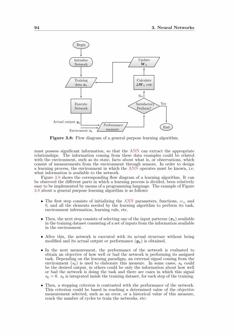
94 3. Neural Networks
Begin
Initialize
Network
Update
W k
Training
data xk
Calculate
∆W k rule
Execute
Network
Satisfactory
Perform?
Performance
measureEnd
Actual output yk
Enviroment sk
No
Yes
Figure 3.8: Flow diagram of a general purpose learning algorithm.
must possess significant information, so that the ANN can extract the appropriaterelationships. The information coming from these data examples could be relatedwith the environment, such as its state, facts about what is, or observations, whichconsist of measurements from the environment through sensors. In order to designa learning process, the environment in which the ANN operates must be known, i.e.what information is available to the network.
Figure 3.8 shows the corresponding flow diagram of a learning algorithm. It canbe observed the different parts in which a learning process is divided, been relativelyeasy to be implemented by means of a programming language. The example of Figure3.8 about a general purpose learning algorithm is as follows:
The first step consists of initializing the ANN parameters, functions, wij andθi and all the elements needed by the learning algorithm to perform its task,environment information, learning rule, etc.
Then, the next step consists of selecting one of the input patterns (xk) availablein the training dataset consisting of a set of inputs from the information availablein the environment.
After this, the network is executed with its actual structure without beingmodified and its actual output or performance (yk) is obtained.
In the next measurement, the performance of the network is evaluated toobtain an objective of how well or bad the network is performing its assignedtask. Depending on the learning paradigm, an external signal coming from theenvironment (sk) is used to elaborate this measure. In some cases, sk couldbe the desired output, in others could be only the information about how wellor bad the network is doing the task and there are cases in which this signalsk = 0. sk is integrated inside the training dataset, for each step of the training.
Then, a stopping criterion is contrasted with the performance of the network.This criterion could be based in reaching a determined value of the objectivemeasurement selected, such as an error, or a historical value of this measure,reach the number of cycles to train the networks, etc:

3.5. How to train your ANN: Learning vs. Tuning 95
– If the network exceeds this criterion, then the learning process ends.Otherwise, the learning process continues and it is necessary that thenetwork assimilates the result of the objective measurement into itsstructure.
– In case that the stopping criteria is not satisfied, it is necessary to calculatethe modification of the free parameters of the network, ∆W k, taking intoaccount the measurements done previously.
Finally, the structure of the network is modified by following ∆W k and a newstep of the training begins by taking the next example inside the training dataset.
Those are the common steps in a general purpose learning algorithm and the nameof a complete cycle is called “epoch”. There are different existing learning algorithms,but all of them follow a structure similar to the one of Figure 3.8. However, notall of them apply these steps in the same order, or the information coming fromthe environment is different or simply use a different variable to update and changethe behavior of the network. Thus, there exists a vast amount of different learningalgorithms. In any case, the versatility provided by learning algorithms makes possiblethat ANNs perform almost any task whenever there are enough training data andenough time to train them. In Sections 3.5.1.1 and 3.5.1.2, different types of trainingand some concerns to consider when training an ANN are presented.
3.5.1.1 Types and rules
This Section introduces different types of learning algorithms and the rules theyuse to modify the different free parameters. In Section 3.2, when classifying thedifferent neural architectures, three different paradigms of learning were introduced:supervised, unsupervised and reinforcement. The difference between them is how thealgorithm interacts with the environment and how much information is obtained fromit. Therefore, from Section 3.2, the definition of each learning paradigm is (Jain et al.,1996; Haykin, 2009):
Supervised. It is also called learning from a teacher. In this type of learning,the ANN is provided with information about the desired output of the systemfor each input. The modification of the weights is based on the deviation of theANN output from the desired output for the given input.
Unsupervised. There is no environmental signal sk coming from the outside, theonly information available is the set of inputs. This learning algorithm exploresthe structure in the data to detect similarities among them, doing correlationsbetween patterns in the data, and organizing them into categories from thesecorrelations.
Reinforcement. As in supervised learning, there is information coming fromthe environment about the performance of the network. But rather than usingthe desired output, the network is provided with only an observation on thecorrectness of ANN outputs or possibly, how right or wrong the ANN outputwas. Thus, there is not an exact measure of the error, only information aboutthe performance of the network.
Each of these algorithms can be used alone or combinations of them using hybridlearning algorithms, in which different learning strategies can be used to train differentparts of the ANN. The more biologically plausible of all these learning paradigms isthe unsupervised learning, because only the input is given to the network and it is theANN which establishes the relationships among the data. However, this paradigm isnot suitable for all the problems. In contrast, reinforcement and supervised learninghave information from the environment, consisting of how well the ANN is doing itstask, but in reinforcement it is less precise than in supervised learning. Supervised
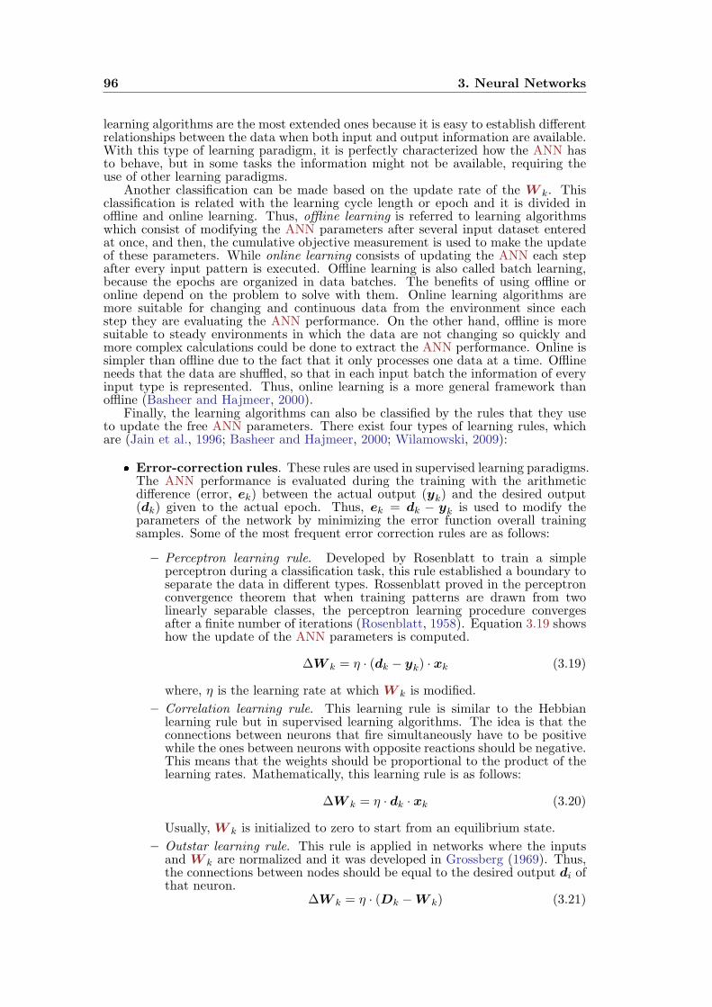
96 3. Neural Networks
learning algorithms are the most extended ones because it is easy to establish differentrelationships between the data when both input and output information are available.With this type of learning paradigm, it is perfectly characterized how the ANN hasto behave, but in some tasks the information might not be available, requiring theuse of other learning paradigms.
Another classification can be made based on the update rate of the W k. Thisclassification is related with the learning cycle length or epoch and it is divided inoffline and online learning. Thus, offline learning is referred to learning algorithmswhich consist of modifying the ANN parameters after several input dataset enteredat once, and then, the cumulative objective measurement is used to make the updateof these parameters. While online learning consists of updating the ANN each stepafter every input pattern is executed. Offline learning is also called batch learning,because the epochs are organized in data batches. The benefits of using offline oronline depend on the problem to solve with them. Online learning algorithms aremore suitable for changing and continuous data from the environment since eachstep they are evaluating the ANN performance. On the other hand, offline is moresuitable to steady environments in which the data are not changing so quickly andmore complex calculations could be done to extract the ANN performance. Online issimpler than offline due to the fact that it only processes one data at a time. Offlineneeds that the data are shuffled, so that in each input batch the information of everyinput type is represented. Thus, online learning is a more general framework thanoffline (Basheer and Hajmeer, 2000).
Finally, the learning algorithms can also be classified by the rules that they useto update the free ANN parameters. There exist four types of learning rules, whichare (Jain et al., 1996; Basheer and Hajmeer, 2000; Wilamowski, 2009):
Error-correction rules. These rules are used in supervised learning paradigms.The ANN performance is evaluated during the training with the arithmeticdifference (error, ek) between the actual output (yk) and the desired output(dk) given to the actual epoch. Thus, ek = dk − yk is used to modify theparameters of the network by minimizing the error function overall trainingsamples. Some of the most frequent error correction rules are as follows:
– Perceptron learning rule. Developed by Rosenblatt to train a simpleperceptron during a classification task, this rule established a boundary toseparate the data in different types. Rossenblatt proved in the perceptronconvergence theorem that when training patterns are drawn from twolinearly separable classes, the perceptron learning procedure convergesafter a finite number of iterations (Rosenblatt, 1958). Equation 3.19 showshow the update of the ANN parameters is computed.
∆W k = η · (dk − yk) · xk (3.19)
where, η is the learning rate at which W k is modified.
– Correlation learning rule. This learning rule is similar to the Hebbianlearning rule but in supervised learning algorithms. The idea is that theconnections between neurons that fire simultaneously have to be positivewhile the ones between neurons with opposite reactions should be negative.This means that the weights should be proportional to the product of thelearning rates. Mathematically, this learning rule is as follows:
∆W k = η · dk · xk (3.20)
Usually, W k is initialized to zero to start from an equilibrium state.
– Outstar learning rule. This rule is applied in networks where the inputsand W k are normalized and it was developed in Grossberg (1969). Thus,the connections between nodes should be equal to the desired output di ofthat neuron.
∆W k = η · (Dk −W k) (3.21)
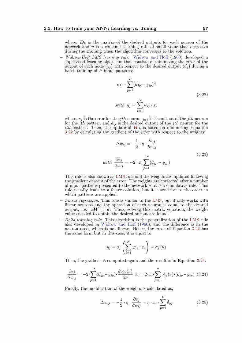
3.5. How to train your ANN: Learning vs. Tuning 97
where, Dk is the matrix of the desired outputs for each neuron of thenetwork and η is a constant learning rate of small value that decreasesduring the training when the algorithm converges to the solution.
– Widrow-Hoff LMS learning rule. Widrow and Hoff (1960) developed asupervised learning algorithm that consists of minimizing the error of theoutput of each node (yj) with respect to the desired output (dj) during abatch training of P input patterns:
ej =
P∑p=1
(djp − yjp)2
with yj =
N∑i=1
wij · xi
(3.22)
where, ej is the error for the jth neuron, yij is the output of the jth neuronfor the ith pattern and dij is the desired output of the jth neuron for theith pattern. Then, the update of W k is based on minimizing Equation3.22 by calculating the gradient of the error with respect to the weights:
∆wij = −1
2· η · ∂ej
∂wij
with∂ej∂wij
= −2 · xiP∑
p=1
(djp − yjp)
(3.23)
This rule is also known as LMS rule and the weights are updated followingthe gradient descent of the error. The weights are corrected after a numberof input patterns presented to the network so it is a cumulative rule. Thisrule usually leads to a faster solution, but it is sensitive to the order inwhich patterns are applied.
– Linear regression. This rule is similar to the LMS, but it only works withlinear neurons and the operation of each neuron is equal to the desiredoutput, i.e. xW = d. Thus, solving this matrix equation, the weightvalues needed to obtain the desired output are found.
– Delta learning rule. This algorithm is the generalization of the LMS rulealso developed in Widrow and Hoff (1960), and the difference is in theneuron used, which is not linear. Hence, the error of Equation 3.22 hasthe same form but in this case, it is equal to
yj = σj
(N∑i=1
wij · xi
)= σj (ν)
Then, the gradient is computed again and the result is in Equation 3.24.
∂ej∂wij
= −2·P∑
p=1
(djp−yjp)·∂σjp(ν)
∂ν·xi = 2·xi ·
P∑p=1
σ′jp(ν)·(djp−yjp) (3.24)
Finally, the modification of the weights is calculated as,
∆wij = −1
2· η · ∂ej
∂wij= η · xi ·
P∑p=1
δpj (3.25)
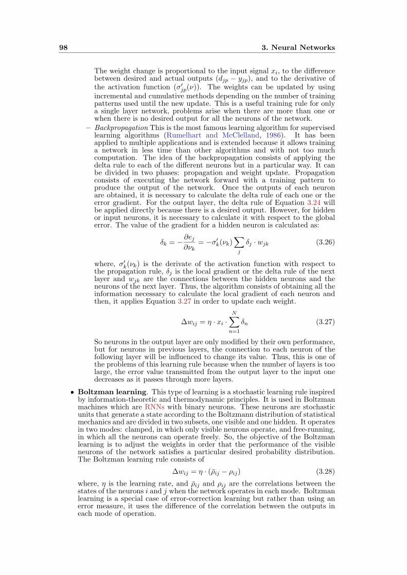
98 3. Neural Networks
The weight change is proportional to the input signal xi, to the differencebetween desired and actual outputs (djp − yjp), and to the derivative ofthe activation function (σ′
jp(ν)). The weights can be updated by usingincremental and cumulative methods depending on the number of trainingpatterns used until the new update. This is a useful training rule for onlya single layer network, problems arise when there are more than one orwhen there is no desired output for all the neurons of the network.
– Backpropagation This is the most famous learning algorithm for supervisedlearning algorithms (Rumelhart and McClelland, 1986). It has beenapplied to multiple applications and is extended because it allows traininga network in less time than other algorithms and with not too muchcomputation. The idea of the backpropagation consists of applying thedelta rule to each of the different neurons but in a particular way. It canbe divided in two phases: propagation and weight update. Propagationconsists of executing the network forward with a training pattern toproduce the output of the network. Once the outputs of each neuronare obtained, it is necessary to calculate the delta rule of each one or theerror gradient. For the output layer, the delta rule of Equation 3.24 willbe applied directly because there is a desired output. However, for hiddenor input neurons, it is necessary to calculate it with respect to the globalerror. The value of the gradient for a hidden neuron is calculated as:
δk = −∂ej∂νk
= −σ′k(νk)
∑j
δj · wjk (3.26)
where, σ′k(νk) is the derivate of the activation function with respect to
the propagation rule, δj is the local gradient or the delta rule of the nextlayer and wjk are the connections between the hidden neurons and theneurons of the next layer. Thus, the algorithm consists of obtaining all theinformation necessary to calculate the local gradient of each neuron andthen, it applies Equation 3.27 in order to update each weight.
∆wij = η · xi ·N∑
n=1
δn (3.27)
So neurons in the output layer are only modified by their own performance,but for neurons in previous layers, the connection to each neuron of thefollowing layer will be influenced to change its value. Thus, this is one ofthe problems of this learning rule because when the number of layers is toolarge, the error value transmitted from the output layer to the input onedecreases as it passes through more layers.
Boltzman learning. This type of learning is a stochastic learning rule inspiredby information-theoretic and thermodynamic principles. It is used in Boltzmanmachines which are RNNs with binary neurons. These neurons are stochasticunits that generate a state according to the Boltzmann distribution of statisticalmechanics and are divided in two subsets, one visible and one hidden. It operatesin two modes: clamped, in which only visible neurons operate, and free-running,in which all the neurons can operate freely. So, the objective of the Boltzmanlearning is to adjust the weights in order that the performance of the visibleneurons of the network satisfies a particular desired probability distribution.The Boltzman learning rule consists of
∆wij = η · (ρij − ρij) (3.28)
where, η is the learning rate, and ρij and ρij are the correlations between thestates of the neurons i and j when the network operates in each mode. Boltzmanlearning is a special case of error-correction learning but rather than using anerror measure, it uses the difference of the correlation between the outputs ineach mode of operation.
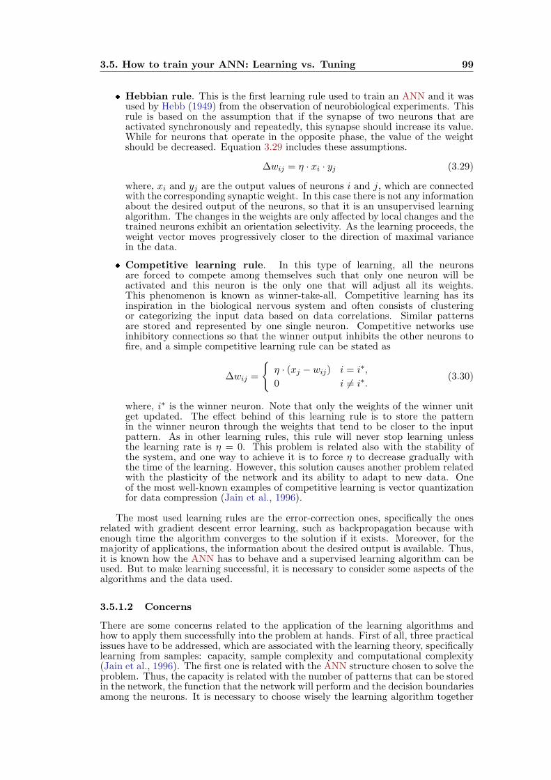
3.5. How to train your ANN: Learning vs. Tuning 99
Hebbian rule. This is the first learning rule used to train an ANN and it wasused by Hebb (1949) from the observation of neurobiological experiments. Thisrule is based on the assumption that if the synapse of two neurons that areactivated synchronously and repeatedly, this synapse should increase its value.While for neurons that operate in the opposite phase, the value of the weightshould be decreased. Equation 3.29 includes these assumptions.
∆wij = η · xi · yj (3.29)
where, xi and yj are the output values of neurons i and j, which are connectedwith the corresponding synaptic weight. In this case there is not any informationabout the desired output of the neurons, so that it is an unsupervised learningalgorithm. The changes in the weights are only affected by local changes and thetrained neurons exhibit an orientation selectivity. As the learning proceeds, theweight vector moves progressively closer to the direction of maximal variancein the data.
Competitive learning rule. In this type of learning, all the neuronsare forced to compete among themselves such that only one neuron will beactivated and this neuron is the only one that will adjust all its weights.This phenomenon is known as winner-take-all. Competitive learning has itsinspiration in the biological nervous system and often consists of clusteringor categorizing the input data based on data correlations. Similar patternsare stored and represented by one single neuron. Competitive networks useinhibitory connections so that the winner output inhibits the other neurons tofire, and a simple competitive learning rule can be stated as
∆wij =
η · (xj − wij) i = i∗,
0 i = i∗.(3.30)
where, i∗ is the winner neuron. Note that only the weights of the winner unitget updated. The effect behind of this learning rule is to store the patternin the winner neuron through the weights that tend to be closer to the inputpattern. As in other learning rules, this rule will never stop learning unlessthe learning rate is η = 0. This problem is related also with the stability ofthe system, and one way to achieve it is to force η to decrease gradually withthe time of the learning. However, this solution causes another problem relatedwith the plasticity of the network and its ability to adapt to new data. Oneof the most well-known examples of competitive learning is vector quantizationfor data compression (Jain et al., 1996).
The most used learning rules are the error-correction ones, specifically the onesrelated with gradient descent error learning, such as backpropagation because withenough time the algorithm converges to the solution if it exists. Moreover, for themajority of applications, the information about the desired output is available. Thus,it is known how the ANN has to behave and a supervised learning algorithm can beused. But to make learning successful, it is necessary to consider some aspects of thealgorithms and the data used.
3.5.1.2 Concerns
There are some concerns related to the application of the learning algorithms andhow to apply them successfully into the problem at hands. First of all, three practicalissues have to be addressed, which are associated with the learning theory, specificallylearning from samples: capacity, sample complexity and computational complexity(Jain et al., 1996). The first one is related with the ANN structure chosen to solve theproblem. Thus, the capacity is related with the number of patterns that can be storedin the network, the function that the network will perform and the decision boundariesamong the neurons. It is necessary to choose wisely the learning algorithm together
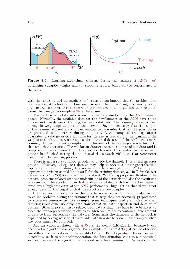
100 3. Neural Networks
W′
W1 W
∗
W2
Globalminimum
Localminimum
W
e(W )
(a)
Epoch
e(y)
Training
TestingOptimum
(b)
Figure 3.9: Learning algorithms concerns during the training of ANNs: (a)
initializing synaptic weights and (b) stopping criteria based on the performance of
the ANN.
with the structure and the application because it can happen that the problem doesnot have a solution for the combination. For example, underfitting problems typicallyoccurred when the error of the network performance is too high, and they could becaused by using a too simple ANN architecture.
The next issue to take into account is the data used during the ANN trainingphase. Normally, the available data for the development of the ANN have to bedivided in three datasets: training, test and validation. The training dataset is usedduring the weight update phase of the network. So, it is necessary that the samplesof the training dataset are complex enough to guarantee that all the possibilitiesare presented to the network during this phase. A well-composed training datasetguarantees a valid generalization. The test dataset is used during the training of theweights to check the network response for untrained data and if the ANN needs moretraining. It has different examples from the ones of the training dataset but withthe same characteristics. The validation dataset contains the rest of the data and iscomposed of data different from the other two datasets. It is used when the learningprocess has finished testing the abilities of the network with data that were neverused during the learning process.
There is not a rule to follow in order to divide the dataset. It is a trial an errorprocess. However, a large test dataset may help to obtain a better generalizationcapability, but the remaining datasets may not have enough data. Particularly, anappropriate division should be 40–50% for the training dataset, 30–40% for the testdataset and a 10–20% for the validation dataset. With an appropriate division of thedataset, problems related with the underfitting of the network and also the overfittingproblem could be avoided. This last problem is related with having a low trainingerror but a high test error of the ANN performance, highlighting that there is notenough data for training it or that the structure is too complex.
It is also very important that the data have the proper form and is adequate tosolve the problem during the training that is why they are normally preprocessedto accelerate convergence. For example, some techniques used are: noise removal,reducing input dimensionality, data transformation, data inspection and deletion ofoutliers. Other important issue related with data is that they have to be balanced toavoid the over-representation of one class. Moreover, it has to contain a large amountof data to train successfully the network. Sometimes the database of the network isexpanded by adding noise to the available data in order to obtain new examples whennew ones cannot be obtained.
Another concern related with ANNs is the weight initialization because it canaffect to the algorithm convergence. For example, in Figure 3.9(a), it can be observedtwo different initializations of the weights W 1 and W 2. In gradient descent learningalgorithms, such as the backpropagation, the first situation leads to a suboptimalsolution because the algorithm is trapped in a local minimum. Whereas in the
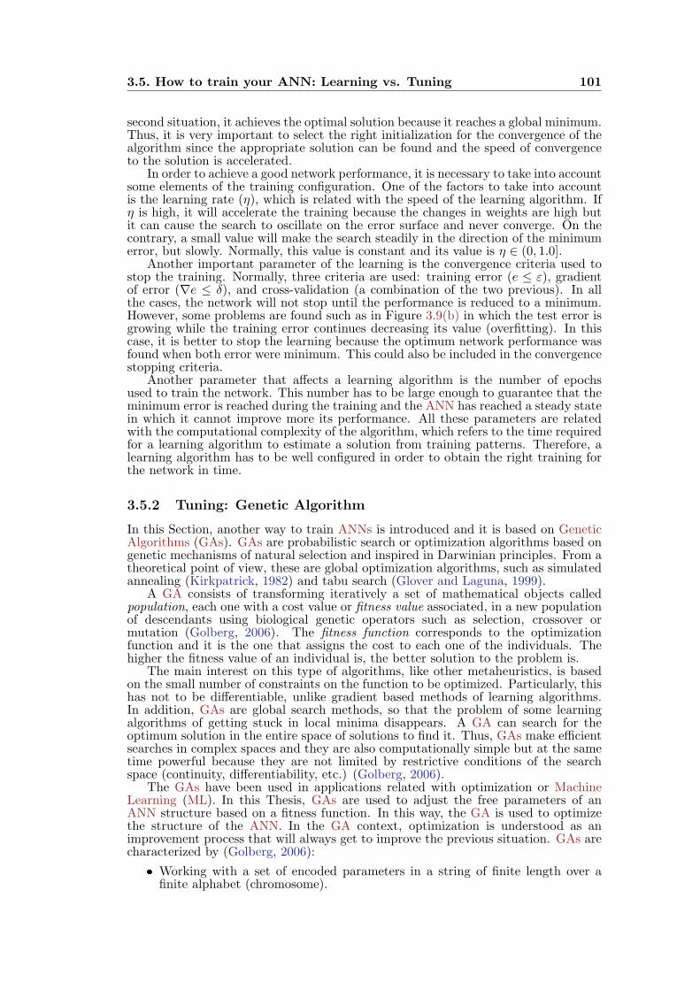
3.5. How to train your ANN: Learning vs. Tuning 101
second situation, it achieves the optimal solution because it reaches a global minimum.Thus, it is very important to select the right initialization for the convergence of thealgorithm since the appropriate solution can be found and the speed of convergenceto the solution is accelerated.
In order to achieve a good network performance, it is necessary to take into accountsome elements of the training configuration. One of the factors to take into accountis the learning rate (η), which is related with the speed of the learning algorithm. Ifη is high, it will accelerate the training because the changes in weights are high butit can cause the search to oscillate on the error surface and never converge. On thecontrary, a small value will make the search steadily in the direction of the minimumerror, but slowly. Normally, this value is constant and its value is η ∈ (0, 1.0].
Another important parameter of the learning is the convergence criteria used tostop the training. Normally, three criteria are used: training error (e ≤ ε), gradientof error (∇e ≤ δ), and cross-validation (a combination of the two previous). In allthe cases, the network will not stop until the performance is reduced to a minimum.However, some problems are found such as in Figure 3.9(b) in which the test error isgrowing while the training error continues decreasing its value (overfitting). In thiscase, it is better to stop the learning because the optimum network performance wasfound when both error were minimum. This could also be included in the convergencestopping criteria.
Another parameter that affects a learning algorithm is the number of epochsused to train the network. This number has to be large enough to guarantee that theminimum error is reached during the training and the ANN has reached a steady statein which it cannot improve more its performance. All these parameters are relatedwith the computational complexity of the algorithm, which refers to the time requiredfor a learning algorithm to estimate a solution from training patterns. Therefore, alearning algorithm has to be well configured in order to obtain the right training forthe network in time.
3.5.2 Tuning: Genetic Algorithm
In this Section, another way to train ANNs is introduced and it is based on GeneticAlgorithms (GAs). GAs are probabilistic search or optimization algorithms based ongenetic mechanisms of natural selection and inspired in Darwinian principles. From atheoretical point of view, these are global optimization algorithms, such as simulatedannealing (Kirkpatrick, 1982) and tabu search (Glover and Laguna, 1999).
A GA consists of transforming iteratively a set of mathematical objects calledpopulation, each one with a cost value or fitness value associated, in a new populationof descendants using biological genetic operators such as selection, crossover ormutation (Golberg, 2006). The fitness function corresponds to the optimizationfunction and it is the one that assigns the cost to each one of the individuals. Thehigher the fitness value of an individual is, the better solution to the problem is.
The main interest on this type of algorithms, like other metaheuristics, is basedon the small number of constraints on the function to be optimized. Particularly, thishas not to be differentiable, unlike gradient based methods of learning algorithms.In addition, GAs are global search methods, so that the problem of some learningalgorithms of getting stuck in local minima disappears. A GA can search for theoptimum solution in the entire space of solutions to find it. Thus, GAs make efficientsearches in complex spaces and they are also computationally simple but at the sametime powerful because they are not limited by restrictive conditions of the searchspace (continuity, differentiability, etc.) (Golberg, 2006).
The GAs have been used in applications related with optimization or MachineLearning (ML). In this Thesis, GAs are used to adjust the free parameters of anANN structure based on a fitness function. In this way, the GA is used to optimizethe structure of the ANN. In the GA context, optimization is understood as animprovement process that will always get to improve the previous situation. GAs arecharacterized by (Golberg, 2006):
Working with a set of encoded parameters in a string of finite length over afinite alphabet (chromosome).
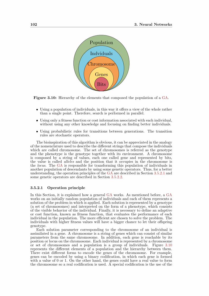
102 3. Neural Networks
Bits
Population
Indviduals
Chromosome
Genes
Figure 3.10: Hierarchy of the elements that composed the population of a GA.
Using a population of individuals, in this way it offers a view of the whole ratherthan a single point. Therefore, search is performed in parallel.
Using only a fitness function or cost information associated with each individual,without using any other knowledge and focusing on finding better individuals.
Using probabilistic rules for transitions between generations. The transitionrules are stochastic operators.
The bioinspiration of this algorithm is obvious, it can be appreciated in the analogyof the nomenclature used to describe the different strings that compose the individualswhich are called chromosome. The set of chromosomes is referred as the genotypeand the phenotype is the genotype together with its environment. A chromosomeis composed by a string of values, each one called gene and represented by bits,the value is called alleles and the position that it occupies in the chromosome isthe locus. The GA is responsible for transforming this population of individuals inanother population of descendants by using some genetic operators. Thus, for a betterunderstanding, the operation principles of the GA are described in Section 3.5.2.1 andsome genetic operators are described in Section 3.5.2.2.
3.5.2.1 Operation principle
In this Section, it is explained how a general GA works. As mentioned before, a GAworks on an initially random population of individuals and each of them represents asolution of the problem in which is applied. Each solution is represented by a genotype(a set of chromosomes) and interpreted on the form of a phenotype, which consistsof the visible behavior of the individual. Finally, it is necessary to define an adaptiveor cost function, known as fitness function, that evaluates the performance of eachindividual in the population. The more efficient are chosen to solve the problem. Theindividuals with higher fitness values will have a bigger chance to let their offspringgenotype.
Each solution parameter corresponding to the chromosome of an individual isassimilated in a gene. A chromosome is a string of genes which can consist of similarparameters from the same chromosome. In addition, each gene is reachable by itsposition or locus on the chromosome. Each individual is represented by a chromosomeor set of chromosomes and a population is a group of individuals. Figure 3.10represents the different elements of a population and the hierarchy between them.There exist different forms to encode the genes of the chromosome. For example,genes can be encoded by using a binary codification, in which each gene is formedwith a value of 0 or 1. On the other hand, the genes could have a real value to formthe chromosome so a real codification is used. A special codification is the use of the
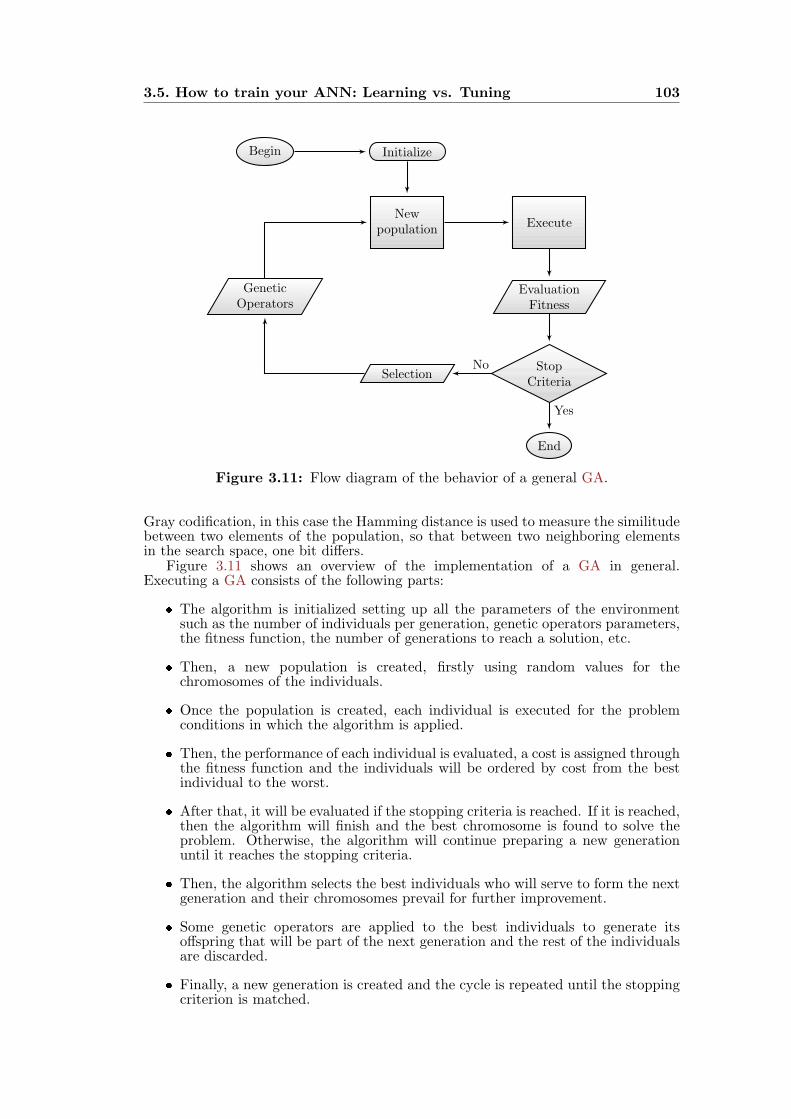
3.5. How to train your ANN: Learning vs. Tuning 103
Begin Initialize
New
populationExecute
Genetic
OperatorsEvaluation
Fitness
SelectionStop
Criteria
End
Yes
No
Figure 3.11: Flow diagram of the behavior of a general GA.
Gray codification, in this case the Hamming distance is used to measure the similitudebetween two elements of the population, so that between two neighboring elementsin the search space, one bit differs.
Figure 3.11 shows an overview of the implementation of a GA in general.Executing a GA consists of the following parts:
The algorithm is initialized setting up all the parameters of the environmentsuch as the number of individuals per generation, genetic operators parameters,the fitness function, the number of generations to reach a solution, etc.
Then, a new population is created, firstly using random values for thechromosomes of the individuals.
Once the population is created, each individual is executed for the problemconditions in which the algorithm is applied.
Then, the performance of each individual is evaluated, a cost is assigned throughthe fitness function and the individuals will be ordered by cost from the bestindividual to the worst.
After that, it will be evaluated if the stopping criteria is reached. If it is reached,then the algorithm will finish and the best chromosome is found to solve theproblem. Otherwise, the algorithm will continue preparing a new generationuntil it reaches the stopping criteria.
Then, the algorithm selects the best individuals who will serve to form the nextgeneration and their chromosomes prevail for further improvement.
Some genetic operators are applied to the best individuals to generate itsoffspring that will be part of the next generation and the rest of the individualsare discarded.
Finally, a new generation is created and the cycle is repeated until the stoppingcriterion is matched.

104 3. Neural Networks
There are some considerations that have to be taken into account when using GAs.The core piece of the GA is the fitness function. When using a GA, it is necessarythat this function is well defined with respect to the problem, otherwise the GA willnot be able to solve it or will have difficulty converging at all. The design of a fitnessfunction is a complex process, so that it is normally used in applications where theproblem is well identified. Moreover, the fitness function evaluation is related with thetime that the algorithm requires solving the problem. Thus, for complex problems,the fitness evaluation is large and it is limiting the algorithm. In addition, GAs with afitness function with abrupt changes between two states, such as in decision problems,are not able to converge to the solution because of the oscillation in the solutions.
The stopping criterion is another issue of GA. Normally, the GA will be workinggeneration after generation until it finds the best possible solution of the problem andobtains the highest value of the fitness. However, a stopping criterion is usually usedbased on the stuck value of the fitness during a number of generations in combinationwith a maximum number of generations. Finally, selection and other operators of theGA are presented in Section 3.5.2.2.
3.5.2.2 Genetic operators
Three main genetic operators are: selection, crossover and mutation. They are appliedbetween generations to form the next one. First the individuals are selected accordingto their fitness value, then the crossover is applied between chromosomes and finally,the mutation is in charge of altering some genes.
The selection operator is responsible for defining which individuals of the currentpopulation will be used in the new population of the next generation, which willserve as parents during the crossover operation. This operator can be considered themost important because it allows individuals in a population to survive, reproduceor die. In general, the probability of survival of an individual is directly related totheir relative effectiveness within the population, i.e. its fitness value. Four types ofselection methods are introduced (Golberg, 2006).
Roulette-wheel selection. This method is the most used. With this selectionmethod, each individual has a chance of being selected proportional to itsperformance. Thus, the fittest individuals are the ones that have higherprobabilities to be selected to breed the next generation. Imagine a roulette orwheel, each individual is associated with a sector whose size is proportional toits fitness value. This selection has some drawbacks because of the variance thatpresents when selecting the individuals that compose the wheel. For example,in n selections, the same individual can be selected to be a parent of the newgeneration and no alteration of the fitness value for the new individual will bereached, leading to a loss of diversity. Moreover, it could also fall in individualswith low fitness in spite of the low probability. Therefore, this selection isnormally combined with other types, to avoid these problems.
Elitism. This method consists of selecting the best n individuals, whichhave the higher values of fitness, to be part of the new population. It isusually combined with the previous selection method to avoid some of theaforementioned problems.
Tournament selection. In this method, two individuals are chosen among thebase population, making them fight. The individual with the highest fitnesshas a probability p to win the fight defined between 0.5 and 1. This process isrepeated until all the individuals of the new generation are selected. Again thevariance of this method is high, and the fact that the probability p increases ordecreases its value, allows increasing or decreasing the selection pressure.
Stochastic universal sampling. It is a technique designed to map the originalfitness value of an individual with its expected fitness value, so that the GA isless susceptible to premature convergence. This selection consists of distributing

3.5. How to train your ANN: Learning vs. Tuning 105
the population in a segment based on the fitness values of its individuals, andthen selecting them based on a set of equidistant points.
The next genetic operator used after the selection is the crossover. This operatorconsists of creating a new offspring from the individuals of the selections that are usedto breed the new individuals of the next generation. Hence, the new individuals afterthe crossover inherit partially the characteristics of their parents. This operator isapplied to a couple of individuals and it is made in two steps. The first one consistsof selecting the individuals and associate them randomly in couples (discarding theelite). And then the crossover occurs in one, two or more points defined on thechromosomes randomly, so each one is separated in different segments. After this,each segment is swapped with the corresponding segment of the other parent with achance of crossing defined. Thus, it can be noted that the number of crossing pointsand the probability of crossing, provides more or less diversity in the GA. An exampleof the crossover operator is as follows, imagine that there are two parents x1 and x2with a chromosome length of five genes.
x1 = 10|011x2 = 01|110
where the crossing point is k = 2 and the new individuals for the next generation are:
x′1 = 10110
x′2 = 01011
This is the simplest crossover operator but other crossover operators moreadvanced are (Golberg, 2006):
Partially matched crossover (PMX). This type of crossover consists of selectingtwo random points inside the chromosome to establish the crossing area ofboth chromosomes. After that, with the parts of the chromosome that are notinvolved in the crossover a permutation of the genes is established. For example,suppose that,
x1 = 9 8 4 | 5 6 7 | 1 3 2 10
x2 = 8 7 1 | 2 3 10 | 9 5 4 6.
Then, the central block is swapped and in the other two blocks per chromosome,the genes are permuted, obtaining
x′1 = 9 8 4 | 2 3 10 | 1 6 5 7
x′2 = 8 10 1 | 5 6 7 | 9 2 4 3.
Order crossover (OX). This operator establishes and area for swapping the genesand then it changes them. Unlike the previous operator, in the areas that arenot exchanged instead of being permuted, the chromosome rearranges itself.For example suppose that,
x1 = 9 8 4 | 5 6 7 | 1 3 2 10
x2 = 8 7 1 | 2 3 10 | 9 5 4 6
when x2 makes the exchange of the values, these values are empty and there isnot any value to fill them.
x2 = 8 − 1 | 2 3 10 | 9 − 4 −and now the chromosome is reordered, putting together the empty spots in theswapping area,
x2 = 2 3 10 | − − − | 9 4 8 1
finally, it is obtained that,
x′1 = 5 6 7 | 2 3 10 | 1 9 8 4
x′2 = 2 3 10 | 5 6 7 | 9 4 8 1.
106 3. Neural Networks
Cycle crossover (CX). This type of crossover is different to the two previous onessince a swap area is not established. In this case, a point of the chromosome ischosen from which there will be no changes at all. Then, the value of the firstgene of the second chromosome is sought. If the value of each gene for the twochromosomes does not match, it has ended and it would change all the genes ofboth chromosomes. Otherwise, it would set the first chromosome gene whosevalue is equal to the first gene of the second and would repeat the operation.An example of this operator is as follows,
x1 = 9 8 1 7 4 5
x2 = 1 2 4 5 9 7
first, it is taken the first gene of x1
x′1 = 9 − − − − −
the value of the first gene of x2 is 1 which is also in x′1, so that it will be fixedin the chromosome,
x′1 = 9 − 1 − − −
the value in x2 corresponding to the position that it has been fixed in x′1 is 4,so it will also be fixed,
x′1 = 9 − 1 − 4 −finally, the value of the gene in x2 is 9 that is already fixed so the cycle is finishedand now the exchange of genes can start,
x′1 = 9 2 1 5 4 7
x′2 = 1 8 4 7 9 5
The crossover operator favors the exploration of the search space. Consideringtwo genes A and B that can be improved by mutation, it is unlikely that the A′
and B′ genes altered by the mutation appear in the same individual. But if oneparent has the gene A′ and the other B′, the crossover operator will combine the twogenes, and thus create a new individual by taking this combination. With this newcombination it is possible that the new individual is more adapted than their parents.The crossover operator allows the mixture of genetic material and accumulation offavorable mutations. But it is possible that the joint action of selection and crossingforbids the convergence to the optimal solution of the problem. Thus, considering apopulation of individuals having a chromosome with a single gene with binary values,if none of the individuals in the initial population has the value 1 for this gene,selection and crossover will not allow the appearance of the other values.
It is in this scenario where the mutation operator arises. This operator consistsof changing the value of a gene randomly with a very low probability to do it. In thecase of binary codification of the chromosome, the mutation only inverts the value ofthe gene in a random location of the chromosome. Thus, mutation modifies randomlythe characteristics of the solution and it allows introducing diversity in the solutionpopulation. Mutation can be interpreted as a noise that interferes with the solution byadding new points in the search space. This operator has three main advantages. Thefirst one is that this operator avoids the phenomenon of genetic drift, when some genesfavored by fortune are used to the detriment of others, and are thus present in thesame place in all chromosomes. It also avoids the risk of the premature convergenceof the algorithm in which all the individuals are exactly the same and imitates localoptima solutions because of the diversity that the operator introduces. And the lastone is that it guarantees the ergodicity property in which each point of the solutionspace can be reached. Random mutations in all positions of the gene mathematicallyguarantee that all the solutions are collected in infinite time, so that it is guaranteedto find the global optimum.
3.6. Conclusion 107
Therefore, a simple GA typically consists of a selection, a crossover and amutation operator to be able to explore the entire solution space. Other complexoperators can be added to GA. For example, diploidy consists of having one or morecouples of chromosomes, each one of them has information of the same functionand will be used to be crossed. The dominance is another operator that is used toeliminate redundancies between two equal chromosomes so that preference is givento a particular value against other values that the gene can take. Inversion consistsof choosing two points inside the chromosome which is cut at such points and thepositions of the ends of the cut section are exchanged. In segregation, during thecrossover, only one of the parents is chosen to be part of the next generation. Andtranslocation which is a crossover inside the chromosome, in which the genes locationis changed.
To sum up, different GA operators have been described in order to explain howthe creation of the next generation is carried out. There are some operators morecomplex than others, but all of them are applied to obtain the best individual thatsolves the problem in the fitness function way. In general, not all the operators areused for the same GA. As mentioned above, the most common GAs are composed bythe three main operators, selection, crossover and mutation. In this Thesis, a GA isgoing to be used to optimize the structure of the ANN selected and to that extent, thegenetic operators used are the basic ones in order to simplify the problem of trainingthe ANN.
3.6 Conclusion
In this Chapter, a deep literature review of the Artificial Neural Networks (ANNs) hasbeen done in order to understand better the advantages and disadvantages of usingthis type of AI algorithms in the management of a grid. In first place, a historicalreview was done to understand the evolution of the ANNs and the different milestonesinvolved in their development. Nowadays, the ANNs are commonly used due totheir appealing properties of distributivity, robustness, generalization, redundancy,adaptivity, etc. One of the main reasons of their intensive use is the capacity ofextracting features for large amount of data, which is a worrying problem in theactual society as more data is gathered from the individuals. ANNs fit perfectly forBig Data Analytics (BDA) and Machine Learning (ML).
The different features of the ANNs were presented together with some importantarchitectures and types. Of particular interest are the Recurrent Neural Networks(RNNs) since they present some dynamics characteristics that help in the constructionof an algorithm that manages the power flows of the grid. Therefore, a part ofthe Chapter was dedicated to understand these type of networks and the stabilityproperties that inherit their structure. The reasons for using them are the presence ofa short memory in the feedback loops of the connection structure and the possibilityto model the dynamic behavior of any system.
After describing the most famous architectures and the ones used in this Thesis, itwas necessary to introduce the different fields of applications. ANNs are used mainlyin classification, data processing, function approximation, optimization, associationand control. However, ANNs can be applied almost to any problem that it is welldefined. Moreover, there are different applications in which ANNs are applied, suchas power systems. Some of these applications are: load forecasting, system security,transient stability, fault diagnosis and economic dispatch.
Finally, it was necessary to explain how ANNs are trained in order to fulfill the taskin which they are applied. Two methods have been explained, learning and tuning.Traditionally, learning algorithms have been used to train ANNs by changing the freeparameters of the network. Depending on the application and the available data, thereexist different approximations to use during the training: supervised, unsupervisedand reinforcement learning. In addition, other classifications were introduced tounderstand different aspects on how the ANNs learn from the environment. However,these algorithms present some concerns such as the initialization of the structureor finding suboptimal solutions to the problem. On the other hand, the Genetic

108
Algorithms (GAs) are used to optimize the ANN structure based on the minimizationof a fitness function defined by the user. In general, three operators are used to obtainthe new individuals of the next generation: selection, crossover and mutation.
In this Part of the Thesis, the general concepts of the electrical grid wereintroduced such as the forms of generation, the transport and distribution ofelectricity, the different consumptions inside the grid, etc. In addition, some problemswith the actual status of the grid were introduced in order to tackle them with theupcoming arrival of the Smart Grid (SG). However, there exist barriers to the SGdeployment, one of them is related with the absence of algorithms to manage thegrid. The needs of the grid will be attended by SG, but it is necessary to developalgorithms that manage not only the power flows but also the information comingfrom the different participants of the grid. Thus, a possible algorithm, the ANNs, wasdetailed for its use in this Thesis with the objective of managing the grid power flowfrom the demand side making possible a SG scenario. Part II develops the solutionfound to control the power flows from a DSM approximation using the conceptsintroduced in this first Part of the Thesis.
PART II
NeuralGrid: An approximation
towards Smart Grid


4Individual Controller
“Everything should be made as simple as possible, but not
simpler.” — Albert Einstein
Working with Artificial Neural Networks (ANNs) in power systems hasbeen long used. However, their application field is centered in tasksrelated with their pattern recognition and forecasting abilities, inorder to handle problems that arise in the grid. In this Part of
the Thesis, the use of ANNs is proposed to manage the local demand of differentgrid elements to smooth their aggregated consumption. However, it is done froma particular point of view focusing on Low Voltage (LV) users instead of using thecapabilities of cutting large grid consumptions. In this way, the security of supply isguaranteed for all users and the operation enhancement of the entire grid.
As mentioned in Section 2.3.4, there exist different Demand Side Management(DSM) techniques to address this issue. They are implemented in the form of differentincentives such as energy savings due to the temporal displacement of loads or gridstatus regulation through the direct load control. The DSM algorithm proposed inthe Thesis is based on the load automation of the local electric behavior of LV users.The followed DSM strategy is applied locally, but its effects impact globally in thesystem. Thus, the different users within the grid are self-organized to contribute tosmooth their aggregated consumption. The implementation of this distributed DSMstrategy is the leitmotiv of this Part of the Thesis. A neural approach is used toimplement it which consists of controlling the local electric behaviour by taking intoaccount the aggregated consumption of the electrical grid, local energy resources anduser requirements.
The use of ANNs allows applying their abilities of signal processing and forecastingto vary the behavior of the grid aggregated consumption. Moreover, their adaptiveand distributed properties make it perfect to implement a possible solution to thiselectric paradigm. Specifically, Recurrent Neural Networks (RNNs) are used totackle this problem, due to its dynamic properties and its short-term memory abilityinherited in its structure. Both are desirable properties to design a DSM controllerthat has to adapt to changes in the environment. However, working with RNNs canbe difficult and computationally slow, especially for large structures. Therefore, asmall RNN structure is sought in order to be implemented in each user, by building amodular system of neural blocks that can be executed no matter the technology. Theneural controller designed is going to extract some features from its inputs by usingtemporal series analysis and adaptive filtering theory.
The interest of developing a DSM algorithm is motivated to find solutions tosome problems of the current electrical grids and as a possible solution to improvethe integration of the next generation of grids or Smart Grid (SG). Thus, the ideais to use the data coming from the current monitoring platform, which is increasingtheir capabilities thanks to the deployment of smart meters, and the local informationavailable from the user. There is no possibility to share information between usersbecause the grid does not allow it and guarantees the anonymity of its users.Therefore, a solution to the problem is elaborated with the minimum informationpossible. It must be guaranteed the integrity of the data coming form the users andthe grid operation enhancement. Herein, lies one of the problems that will be tackled
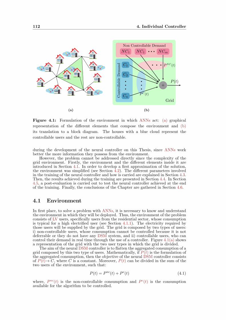
112 4. Individual Controller
(a)
NC1 NC1 NCm
C1
C2
+
Cn
P (t)
Con
trollable
Dem
and
Non Controllable Demand
Grid
PNC(t)
PC(t)
(b)
Figure 4.1: Formulation of the environment in which ANNs act: (a) graphical
representation of the different elements that compose the environment and (b)
its translation to a block diagram. The houses with a blue cloud represent the
controllable users and the rest are non-controllable.
during the development of the neural controller on this Thesis, since ANNs workbetter the more information they possess from the environment.
However, the problem cannot be addressed directly since the complexity of thegrid environment. Firstly, the environment and the different elements inside it areintroduced in Section 4.1. In order to develop a first approximation of the solution,the environment was simplified (see Section 4.2). The different parameters involvedin the training of the neural controller and how is carried are explained in Section 4.3.Then, the results achieved during the training are presented in Section 4.4. In Section4.5, a post-evaluation is carried out to test the neural controller achieved at the endof the training. Finally, the conclusions of the Chapter are gathered in Section 4.6.
4.1 Environment
In first place, to solve a problem with ANNs, it is necessary to know and understandthe environment in which they will be deployed. Thus, the environment of the problemconsists of LV users, specifically users from the residential sector, whose consumptionis typical for a high electrified user (see Section 4.1.1). The electricity required bythose users will be supplied by the grid. The grid is composed by two types of users:i) non-controllable users, whose consumption cannot be controlled because it is notdeferrable or they do not have any DSM system, and ii) controllable users, who cancontrol their demand in real time through the use of a controller. Figure 4.1(a) showsa representation of the grid with the two user types in which the grid is divided.
The aim of the neural DSM controller is to flatten the aggregated consumption of agrid composed by this two type of users. Mathematically, if P (t) is the formulation ofthe aggregated consumption, then the objective of the neural DSM controller consistsof P (t)→ C, where C is a constant. Moreover, P (t) can be divided in the sum of thetwo users of the environment, such that:
P (t) = Pnc(t) + P c(t) (4.1)
where, Pnc(t) is the non-controllable consumption and P c(t) is the consumptionavailable for the algorithm to be controlled.

4.1. Environment 113
without DSM
t
P (t)
t
Pnc(t)
t
Pc(t)
(a)
with DSM
t
P (t)
t
Pnc(t)
t
Pc(t)
(b)
Figure 4.2: Graphical representation of P (t) signal as a sum of Pnc(t) and P c(t)
signals, where: (a) represents the current electric grid where P c(t) is not adapted
to Pnc(t) and (b) represents the proposed algorithm goal where P c(t) is adapted to
Pnc(t) in order to smooth P (t).
Figure 4.1(b) shows a block diagram of the whole system in which the grid has beendivided. These two blocks correspond to the non-controllable and the controllabledemand, which at the same time are subdivided in m and n parts respectively. Thus,each part of the demand, Pnc(t) and P c(t), is represented by the sum of the powerconsumed by each type of user (see Equations 4.2a and 4.2b).
Pnc(t) =m∑i=1
pnci (t) (4.2a) P c(t) =n∑
i=1
pci (t) (4.2b)
where, pnci (t) is the demand of the ith non-controllable user and pci (t) is theconsumption of the ith controllable user.
The electrical behavior of the users and their aggregated consumption is describedin Figure 4.2. In the general case, neither of the users can control their demand so thateach one of them can consume any power at any time as in Figure 4.2(a). In this case,there is no algorithm to control the demand of P c(t) and the aggregated consumptionpossesses a high variability. Thus, it is necessary for the proposed algorithm toreshape the amount of P c(t) in order to adapt to Pnc(t), achieving a flattened P (t)consumption as in Figure 4.2(b). The main challenge, in the design of this type ofalgorithms consists of how to adapt P c(t) to Pnc(t) to produce a flattened response.However, the current information coming from the grid and available by users is non-existent, making difficult the elaboration of a control strategy in order to achieveany goal. Hence, it is necessary to use some techniques already developed in otherfields such as Artificial Intelligence (AI) or signal processing to extract some usefulinformation from the small amount of information provided by the grid.
Information coming from the grid differs from one country to another. Normally,the transmission system operators possess all the information about the demand. Forexample, in Europe the information about the aggregated consumption of differentcountries can be found in European Network of Transmission System Operators(ENTSO-E)1, which represent 41 electricity transmission system operators from 34countries across Europe. In a grid in which users do not control their consumption,the aggregated consumption behaves periodically as shown in Figure 4.3. The data toelaborate Figure 4.3 was obtained from the aggregated consumption of Spain during20152. The aggregated consumption of other countries may differ in the form or inthe power consumed, but the periodicity of valleys and peaks is very similar amongthem because consumption habits among users are very similar. Furthermore, it can
1https://www.entsoe.eu2Source: Red Electrica de Espana (REE), the transmission system operator of Spain.
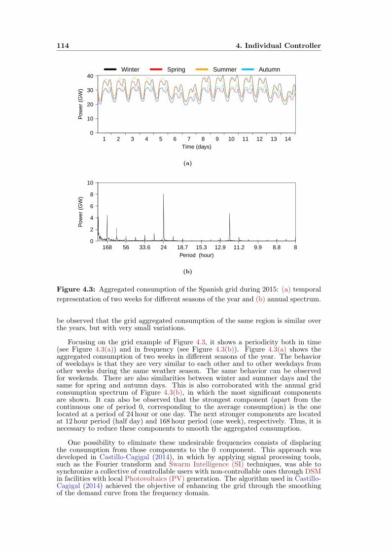
114 4. Individual Controller
0
10
20
30
40
1 2 3 4 5 6 7 8 9 10 11 12 13 14Time (days)
Pow
er (
GW
)
Winter Spring Summer Autumn
(a)
0
2
4
6
8
10
168 56 33.6 24 18.7 15.3 12.9 11.2 9.9 8.8 8Period (hour)
Pow
er (
GW
)
(b)
Figure 4.3: Aggregated consumption of the Spanish grid during 2015: (a) temporal
representation of two weeks for different seasons of the year and (b) annual spectrum.
be observed that the grid aggregated consumption of the same region is similar overthe years, but with very small variations.
Focusing on the grid example of Figure 4.3, it shows a periodicity both in time(see Figure 4.3(a)) and in frequency (see Figure 4.3(b)). Figure 4.3(a) shows theaggregated consumption of two weeks in different seasons of the year. The behaviorof weekdays is that they are very similar to each other and to other weekdays fromother weeks during the same weather season. The same behavior can be observedfor weekends. There are also similarities between winter and summer days and thesame for spring and autumn days. This is also corroborated with the annual gridconsumption spectrum of Figure 4.3(b), in which the most significant componentsare shown. It can also be observed that the strongest component (apart from thecontinuous one of period 0, corresponding to the average consumption) is the onelocated at a period of 24 hour or one day. The next stronger components are locatedat 12 hour period (half day) and 168 hour period (one week), respectively. Thus, it isnecessary to reduce these components to smooth the aggregated consumption.
One possibility to eliminate these undesirable frequencies consists of displacingthe consumption from those components to the 0 component. This approach wasdeveloped in Castillo-Cagigal (2014), in which by applying signal processing tools,such as the Fourier transform and Swarm Intelligence (SI) techniques, was able tosynchronize a collective of controllable users with non-controllable ones through DSMin facilities with local Photovoltaics (PV) generation. The algorithm used in Castillo-Cagigal (2014) achieved the objective of enhancing the grid through the smoothingof the demand curve from the frequency domain.
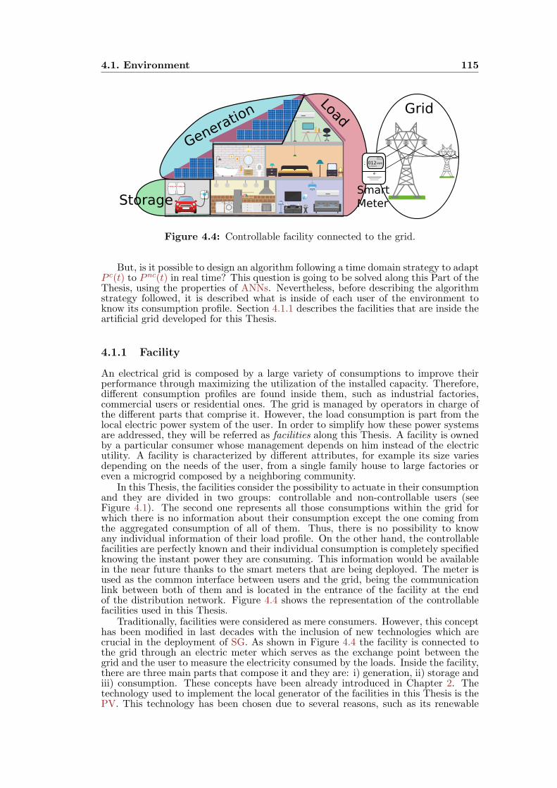
4.1. Environment 115
012kWh
18/03
12:15:00
Id: 29082009
Grid
Generation
LoadStorage
Smart
Meter
Figure 4.4: Controllable facility connected to the grid.
But, is it possible to design an algorithm following a time domain strategy to adaptP c(t) to Pnc(t) in real time? This question is going to be solved along this Part of theThesis, using the properties of ANNs. Nevertheless, before describing the algorithmstrategy followed, it is described what is inside of each user of the environment toknow its consumption profile. Section 4.1.1 describes the facilities that are inside theartificial grid developed for this Thesis.
4.1.1 Facility
An electrical grid is composed by a large variety of consumptions to improve theirperformance through maximizing the utilization of the installed capacity. Therefore,different consumption profiles are found inside them, such as industrial factories,commercial users or residential ones. The grid is managed by operators in charge ofthe different parts that comprise it. However, the load consumption is part from thelocal electric power system of the user. In order to simplify how these power systemsare addressed, they will be referred as facilities along this Thesis. A facility is ownedby a particular consumer whose management depends on him instead of the electricutility. A facility is characterized by different attributes, for example its size variesdepending on the needs of the user, from a single family house to large factories oreven a microgrid composed by a neighboring community.
In this Thesis, the facilities consider the possibility to actuate in their consumptionand they are divided in two groups: controllable and non-controllable users (seeFigure 4.1). The second one represents all those consumptions within the grid forwhich there is no information about their consumption except the one coming fromthe aggregated consumption of all of them. Thus, there is no possibility to knowany individual information of their load profile. On the other hand, the controllablefacilities are perfectly known and their individual consumption is completely specifiedknowing the instant power they are consuming. This information would be availablein the near future thanks to the smart meters that are being deployed. The meter isused as the common interface between users and the grid, being the communicationlink between both of them and is located in the entrance of the facility at the endof the distribution network. Figure 4.4 shows the representation of the controllablefacilities used in this Thesis.
Traditionally, facilities were considered as mere consumers. However, this concepthas been modified in last decades with the inclusion of new technologies which arecrucial in the deployment of SG. As shown in Figure 4.4 the facility is connected tothe grid through an electric meter which serves as the exchange point between thegrid and the user to measure the electricity consumed by the loads. Inside the facility,there are three main parts that compose it and they are: i) generation, ii) storage andiii) consumption. These concepts have been already introduced in Chapter 2. Thetechnology used to implement the local generator of the facilities in this Thesis is thePV. This technology has been chosen due to several reasons, such as its renewable
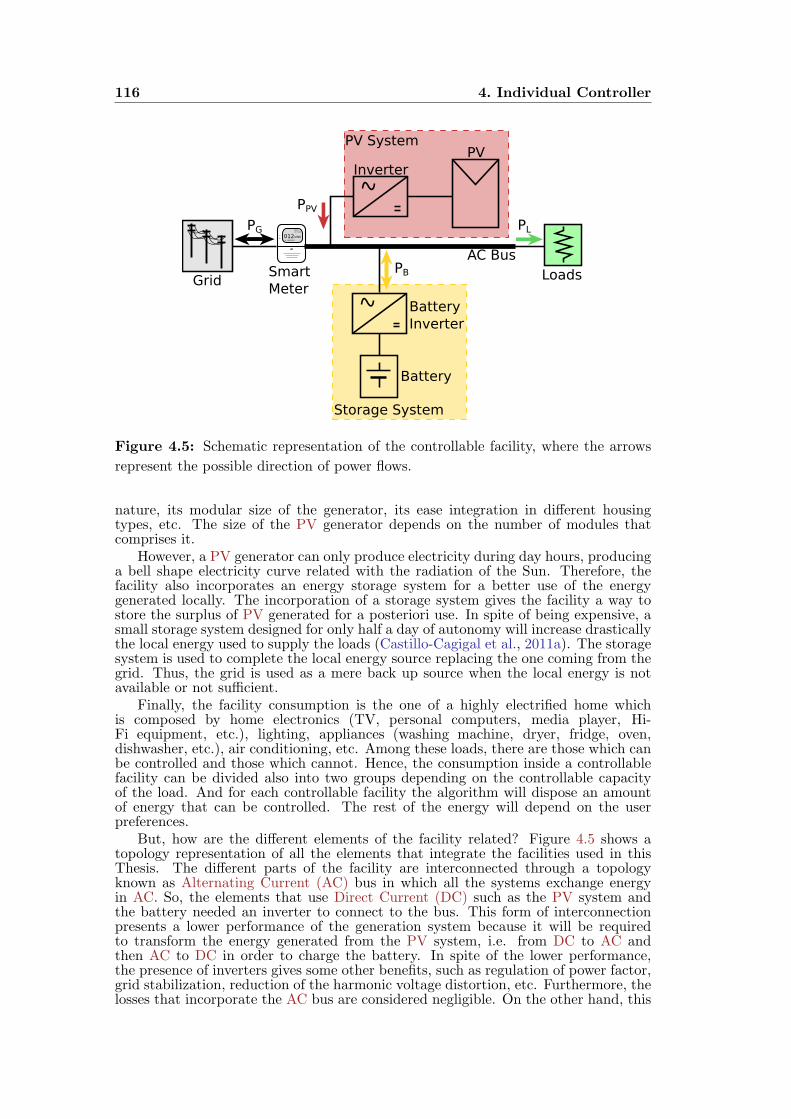
116 4. Individual Controller
012kWh
18/03
12:15:00
Id: 29082009
Smart
MeterLoads
Battery
Inverter
Battery
Storage System
PV SystemPV
Inverter
AC Bus
Grid
PPV
PG
PB
PL
Figure 4.5: Schematic representation of the controllable facility, where the arrows
represent the possible direction of power flows.
nature, its modular size of the generator, its ease integration in different housingtypes, etc. The size of the PV generator depends on the number of modules thatcomprises it.
However, a PV generator can only produce electricity during day hours, producinga bell shape electricity curve related with the radiation of the Sun. Therefore, thefacility also incorporates an energy storage system for a better use of the energygenerated locally. The incorporation of a storage system gives the facility a way tostore the surplus of PV generated for a posteriori use. In spite of being expensive, asmall storage system designed for only half a day of autonomy will increase drasticallythe local energy used to supply the loads (Castillo-Cagigal et al., 2011a). The storagesystem is used to complete the local energy source replacing the one coming from thegrid. Thus, the grid is used as a mere back up source when the local energy is notavailable or not sufficient.
Finally, the facility consumption is the one of a highly electrified home whichis composed by home electronics (TV, personal computers, media player, Hi-Fi equipment, etc.), lighting, appliances (washing machine, dryer, fridge, oven,dishwasher, etc.), air conditioning, etc. Among these loads, there are those which canbe controlled and those which cannot. Hence, the consumption inside a controllablefacility can be divided also into two groups depending on the controllable capacityof the load. And for each controllable facility the algorithm will dispose an amountof energy that can be controlled. The rest of the energy will depend on the userpreferences.
But, how are the different elements of the facility related? Figure 4.5 shows atopology representation of all the elements that integrate the facilities used in thisThesis. The different parts of the facility are interconnected through a topologyknown as Alternating Current (AC) bus in which all the systems exchange energyin AC. So, the elements that use Direct Current (DC) such as the PV system andthe battery needed an inverter to connect to the bus. This form of interconnectionpresents a lower performance of the generation system because it will be requiredto transform the energy generated from the PV system, i.e. from DC to AC andthen AC to DC in order to charge the battery. In spite of the lower performance,the presence of inverters gives some other benefits, such as regulation of power factor,grid stabilization, reduction of the harmonic voltage distortion, etc. Furthermore, thelosses that incorporate the AC bus are considered negligible. On the other hand, this
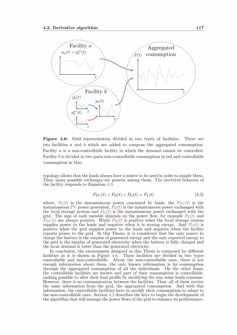
4.2. Derivative algorithm 117
t
pa(t) = pnca(t)
Facility a
t
pcb(t)
t
pncb(t)
t
pb(t)
Facility b t
P (t)
Aggregatedconsumption
Figure 4.6: Grid representation divided in two types of facilities. There are
two facilities a and b which are added to compose the aggregated consumption.
Facility a is a non-controllable facility in which the demand cannot be controlled.
Facility b is divided in two parts non-controllable consumption in red and controllable
consumption in blue.
topology allows that the loads always have a source to be used in order to supply them.Thus, many possible exchanges are present among them. The electrical behavior ofthe facility responds to Equation 4.3:
PPV (t) + PB(t) + PG(t) = PL(t) (4.3)
where, PL(t) is the instantaneous power consumed by loads, the PPV (t) is theinstantaneous PV power generated, PB(t) is the instantaneous power exchanged withthe local storage system and PG(t) is the instantaneous power exchanged with thegrid. The sign of each variable depends on the power flow, for example PL(t) andPPV (t) are always positive. While PB(t) is positive when the local storage systemsupplies power to the loads and negative when it is storing energy. And PG(t) ispositive when the grid supplies power to the loads and negative when the facilityexports power to the grid. In this Thesis, it is considered that the only source tocharge the battery is the surplus of generated energy and the only exported energy tothe grid is the surplus of generated electricity when the battery is fully charged andthe local demand is lower than the generated electricity.
In conclusion, the environment designed in this Thesis is composed by differentfacilities as it is shown in Figure 4.6. These facilities are divided in two typescontrollable and non-controllable. About the non-controllable ones, there is notenough information about them, the only known information is its consumptionthrough the aggregated consumption of all the individuals. On the other hand,the controllable facilities are known and part of their consumption is controllable,making possible to alter their load profile by modifying the way some loads consume.However, there is no communication between the facilities. Thus, all of them receivethe same information from the grid, the aggregated consumption. And with thisinformation, the controllable facilities have to modify their consumption to adapt tothe non-controllable ones. Section 4.2 describes the keys to begin the development ofthe algorithm that will manage the power flows of the grid to enhance its performance.
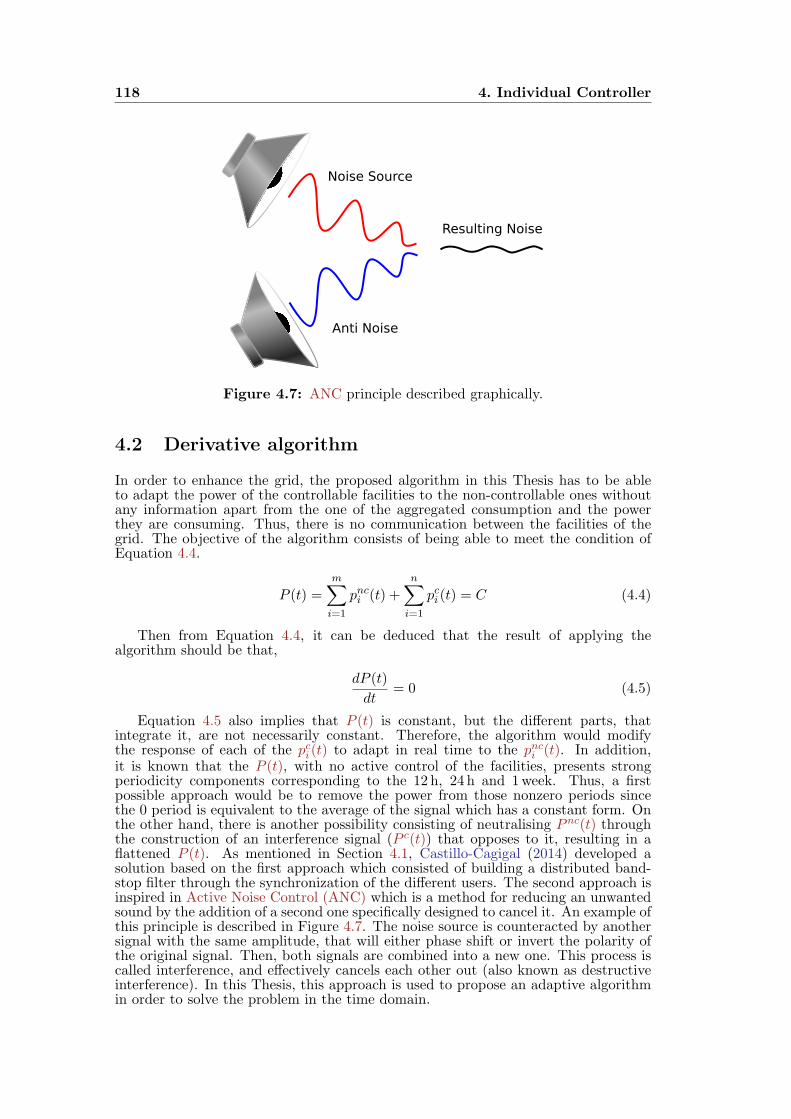
118 4. Individual Controller
Noise Source
Anti Noise
Resulting Noise
Figure 4.7: ANC principle described graphically.
4.2 Derivative algorithm
In order to enhance the grid, the proposed algorithm in this Thesis has to be ableto adapt the power of the controllable facilities to the non-controllable ones withoutany information apart from the one of the aggregated consumption and the powerthey are consuming. Thus, there is no communication between the facilities of thegrid. The objective of the algorithm consists of being able to meet the condition ofEquation 4.4.
P (t) =
m∑i=1
pnci (t) +
n∑i=1
pci (t) = C (4.4)
Then from Equation 4.4, it can be deduced that the result of applying thealgorithm should be that,
dP (t)
dt= 0 (4.5)
Equation 4.5 also implies that P (t) is constant, but the different parts, thatintegrate it, are not necessarily constant. Therefore, the algorithm would modifythe response of each of the pci (t) to adapt in real time to the pnci (t). In addition,it is known that the P (t), with no active control of the facilities, presents strongperiodicity components corresponding to the 12 h, 24 h and 1week. Thus, a firstpossible approach would be to remove the power from those nonzero periods sincethe 0 period is equivalent to the average of the signal which has a constant form. Onthe other hand, there is another possibility consisting of neutralising Pnc(t) throughthe construction of an interference signal (P c(t)) that opposes to it, resulting in aflattened P (t). As mentioned in Section 4.1, Castillo-Cagigal (2014) developed asolution based on the first approach which consisted of building a distributed band-stop filter through the synchronization of the different users. The second approach isinspired in Active Noise Control (ANC) which is a method for reducing an unwantedsound by the addition of a second one specifically designed to cancel it. An example ofthis principle is described in Figure 4.7. The noise source is counteracted by anothersignal with the same amplitude, that will either phase shift or invert the polarity ofthe original signal. Then, both signals are combined into a new one. This process iscalled interference, and effectively cancels each other out (also known as destructiveinterference). In this Thesis, this approach is used to propose an adaptive algorithmin order to solve the problem in the time domain.
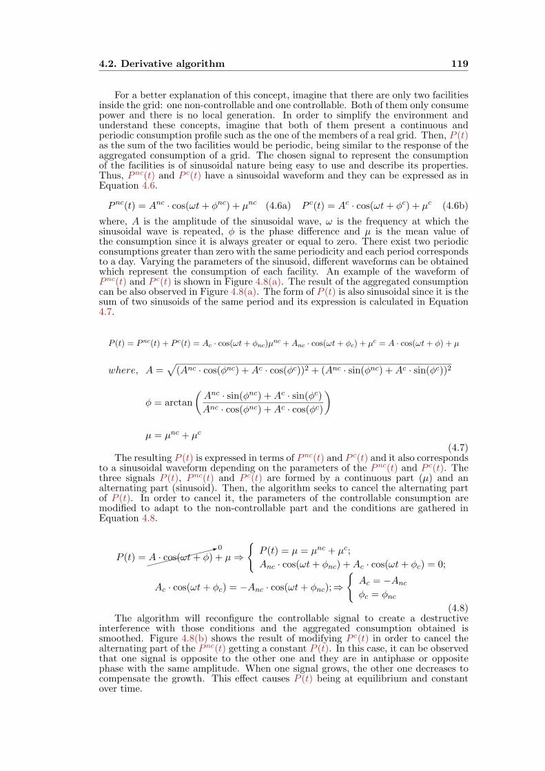
4.2. Derivative algorithm 119
For a better explanation of this concept, imagine that there are only two facilitiesinside the grid: one non-controllable and one controllable. Both of them only consumepower and there is no local generation. In order to simplify the environment andunderstand these concepts, imagine that both of them present a continuous andperiodic consumption profile such as the one of the members of a real grid. Then, P (t)as the sum of the two facilities would be periodic, being similar to the response of theaggregated consumption of a grid. The chosen signal to represent the consumptionof the facilities is of sinusoidal nature being easy to use and describe its properties.Thus, Pnc(t) and P c(t) have a sinusoidal waveform and they can be expressed as inEquation 4.6.
Pnc(t) = Anc · cos(ωt+ ϕnc) + µnc (4.6a) P c(t) = Ac · cos(ωt+ ϕc) + µc (4.6b)
where, A is the amplitude of the sinusoidal wave, ω is the frequency at which thesinusoidal wave is repeated, ϕ is the phase difference and µ is the mean value ofthe consumption since it is always greater or equal to zero. There exist two periodicconsumptions greater than zero with the same periodicity and each period correspondsto a day. Varying the parameters of the sinusoid, different waveforms can be obtainedwhich represent the consumption of each facility. An example of the waveform ofPnc(t) and P c(t) is shown in Figure 4.8(a). The result of the aggregated consumptioncan be also observed in Figure 4.8(a). The form of P (t) is also sinusoidal since it is thesum of two sinusoids of the same period and its expression is calculated in Equation4.7.
P (t) = Pnc(t) + P c(t) = Ac · cos(ωt+ ϕnc)µnc +Anc · cos(ωt+ ϕc) + µc = A · cos(ωt+ ϕ) + µ
where, A =√
(Anc · cos(ϕnc) +Ac · cos(ϕc))2 + (Anc · sin(ϕnc) +Ac · sin(ϕc))2
ϕ = arctan
(Anc · sin(ϕnc) +Ac · sin(ϕc)
Anc · cos(ϕnc) +Ac · cos(ϕc)
)
µ = µnc + µc
(4.7)The resulting P (t) is expressed in terms of Pnc(t) and P c(t) and it also corresponds
to a sinusoidal waveform depending on the parameters of the Pnc(t) and P c(t). Thethree signals P (t), Pnc(t) and P c(t) are formed by a continuous part (µ) and analternating part (sinusoid). Then, the algorithm seeks to cancel the alternating partof P (t). In order to cancel it, the parameters of the controllable consumption aremodified to adapt to the non-controllable part and the conditions are gathered inEquation 4.8.
P (t) =: 0
A · cos(ωt+ ϕ) + µ⇒
P (t) = µ = µnc + µc;
Anc · cos(ωt+ ϕnc) +Ac · cos(ωt+ ϕc) = 0;
Ac · cos(ωt+ ϕc) = −Anc · cos(ωt+ ϕnc);⇒
Ac = −Anc
ϕc = ϕnc
(4.8)The algorithm will reconfigure the controllable signal to create a destructive
interference with those conditions and the aggregated consumption obtained issmoothed. Figure 4.8(b) shows the result of modifying P c(t) in order to cancel thealternating part of the Pnc(t) getting a constant P (t). In this case, it can be observedthat one signal is opposite to the other one and they are in antiphase or oppositephase with the same amplitude. When one signal grows, the other one decreases tocompensate the growth. This effect causes P (t) being at equilibrium and constantover time.
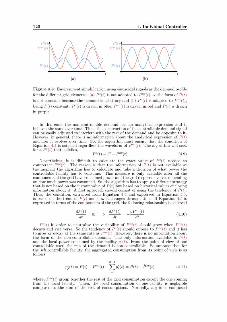
120 4. Individual Controller
Pnc(t)
Pc(t)
P (t)
t
(a)
Pnc(t)
Pc(t)
P (t)
t
(b)
Figure 4.8: Environment simplification using sinusoidal signals as the demand profile
for the different grid elements: (a) P c(t) is not adapted to Pnc(t), so the form of P (t)
is not constant because the demand is arbitrary and (b) P c(t) is adapted to Pnc(t),
being P (t) constant. P c(t) is drawn in blue, Pnc(t) is drawn in red and P (t) is drawn
in purple.
In this case, the non-controllable demand has an analytical expression and itbehaves the same over time. Thus, the construction of the controllable demand signalcan be easily adjusted to interfere with the rest of the demand and be opposite to it.However, in general, there is no information about the analytical expression of P (t)and how it evolves over time. So, the algorithm must ensure that the condition ofEquation 4.4 is satisfied regardless the waveform of Pnc(t). The algorithm will seekfor a P c(t) that satisfies,
P c(t) = C − Pnc(t) (4.9)
Nevertheless, it is difficult to calculate the exact value of P c(t) needed tocounteract Pnc(t). The reason is that the information of P (t) is not available atthe moment the algorithm has to calculate and take a decision of what power thecontrollable facility has to consume. This measure is only available after all thecomponents of the grid have consumed power and the grid response evolves dependingon how much power was consumed. So, the algorithm has to apply a different strategythat is not based on the instant value of P (t) but based on historical values enclosinginformation about it. A first approach should consist of using the tendency of P (t).Thus, the condition, extracted from Equation 4.4 and expressed in Equation 4.5,is based on the trend of P (t) and how it changes through time. If Equation 4.5 isexpressed in terms of the components of the grid, the following relationship is achieved
dP (t)
dt= 0; =⇒ dP c(t)
dt= −dPnc(t)
dt(4.10)
P c(t) in order to neutralise the variability of Pnc(t) should grow when Pnc(t)decays and vice versa. So the tendency of P c(t) should oppose to Pnc(t) and it hasto grow or decay at the same rate as Pnc(t). However, there is no information aboutthe form of the non-controllable demand. The only information available is P (t)and the local power consumed by the facility pci (t). From the point of view of onecontrollable user, the rest of the demand is non-controllable. So suppose that forthe jth controllable facility, the aggregated consumption from its point of view is asfollows
pcj(t) = P (t)− Pnc(t)−n−j∑i=1
pci (t) = P (t)− Pnc(t) (4.11)
where, Pnc(t) group together the rest of the grid consumption except the one comingfrom the local facility. Then, the local consumption of one facility is negligiblecompared to the sum of the rest of consumptions. Normally, a grid is composed
4.3. Neural controller 121
by a huge number of facilities so it is normal that Pnc(t)≈P (t). Thus, a controllablefacility seeks to modify its consumption opposing to the rest of the components ofthe grid. If Equation 4.10 is developed for one individual, it can be obtained that
dpcj(t)
dt= −dPnc(t)
dt≈ −dP (t)
dt(4.12)
In order to reduce the variability of the consumption, one controllable facility hasa trend which is approximately the opposite to the aggregated consumption. Hence,Pnc(t)≈P (t) when the number of individuals of the grid is high. Following the trendof P (t) is the first step to counteract its variability. However, a problem arises whenthe n controllable facilities consume more than the m non-controllable facilities sinceP (t) goes out of the constant equilibrium and a new disturbance has been created.Thus, it is necessary to predict the value of P (t) and adapt to it in order to coordinatethe different controllable facilities. That is why the use of ANN is appropriate andfits perfectly in the development of the proposed algorithm in this Thesis.
As explained in Chapter 3, ANNs have great capacities to act in distributedenvironments. They also stand out in the prediction of temporal series and theirapplication to signal processing problems. In this Thesis, ANNs are used as thealgorithm to manage the different consumptions inside a grid of the characteristicspresented. Therefore, each facility will use a neural controller that has acquired thedynamic behavior of the grid and how to counteract the effects of the rest of the usersbased on the derivate of the aggregated consumption. ANN will know how to opposeto the derivate of P (t) with the only information of the grid signal, P (t), and thelocal behavior of the facility, pci (t). Once the ANN is trained, it will predict the nextinstant value of P (t) and actuate to flatten it.
However, the communication in the environment is restricted and the informationavailable is little. Another challenge to face is how the controllable facilities arecoordinated to smooth the curve. The main reason why they have to act in acoordinated way is because otherwise once the equilibrium is reached, the system couldbe destabilized and P (t) will not be flatten. So, the different neural controllers willself-organize to oppose to the non-controllable demand and stay at the equilibrium.For the rest of the Chapter, it is explained how to build an ANN able to compute thederivative of signal and oppose to an external stimulus. In this case, a restrictedenvironment is used and it is comprised by only one controllable and one non-controllable facility to solve the first part of the problem. Whereas the collectivepart of the algorithm, it will be explained in Chapter 5.
4.3 Neural controller
In this Thesis, the use of ANNs is proposed to build a controller in order to modify thelocal consumption of part of the grid components will produce a smoothed aggregatedconsumption. The only information available is the history of the local consumption,pci (t), and the history of the aggregated consumption, P (t). To produce a flattenedP (t), the idea consists of nullifying its derivative by opposing the amplitude to thenon-controllable consumption. Hence, it is necessary to extract from the data theimportant information and elaborate a response to achieve a constant P (t).
Because of the periodic nature of P (t), an ANN could be applied to do a temporalseries analysis and extract the tendency of P (t) to predict its future values andadapt the response of the facility to achieve a flattened signal. There exist numerousarchitectures of ANNs as it is explained in Chapter 3. However, not all of them arefitted to solve the problem proposed in this Thesis. Thus, it is necessary a versatileANN structure that is able to respond quickly to changes in the environment andadapt to them. There exist a number of structures that possesses these characteristics,being able to model the dynamics of the environment. RNNs fit perfectly for theapplication.
RNNs are commonly used in digital processing applications, but in this casethe reasons to use them are: i) feature extraction in temporal series, ii) forecast
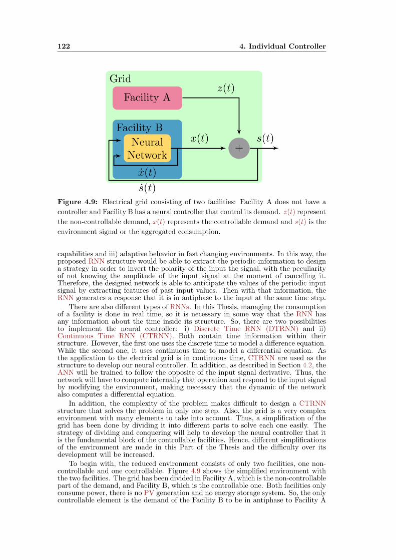
122 4. Individual Controller
Grid
Facility B
Facility A
NeuralNetwork
+
z(t)
x(t)
x(t)
s(t)
s(t)Figure 4.9: Electrical grid consisting of two facilities: Facility A does not have a
controller and Facility B has a neural controller that control its demand. z(t) represent
the non-controllable demand, x(t) represents the controllable demand and s(t) is the
environment signal or the aggregated consumption.
capabilities and iii) adaptive behavior in fast changing environments. In this way, theproposed RNN structure would be able to extract the periodic information to designa strategy in order to invert the polarity of the input the signal, with the peculiarityof not knowing the amplitude of the input signal at the moment of cancelling it.Therefore, the designed network is able to anticipate the values of the periodic inputsignal by extracting features of past input values. Then with that information, theRNN generates a response that it is in antiphase to the input at the same time step.
There are also different types of RNNs. In this Thesis, managing the consumptionof a facility is done in real time, so it is necessary in some way that the RNN hasany information about the time inside its structure. So, there are two possibilitiesto implement the neural controller: i) Discrete Time RNN (DTRNN) and ii)Continuous Time RNN (CTRNN). Both contain time information within theirstructure. However, the first one uses the discrete time to model a difference equation.While the second one, it uses continuous time to model a differential equation. Asthe application to the electrical grid is in continuous time, CTRNN are used as thestructure to develop our neural controller. In addition, as described in Section 4.2, theANN will be trained to follow the opposite of the input signal derivative. Thus, thenetwork will have to compute internally that operation and respond to the input signalby modifying the environment, making necessary that the dynamic of the networkalso computes a differential equation.
In addition, the complexity of the problem makes difficult to design a CTRNNstructure that solves the problem in only one step. Also, the grid is a very complexenvironment with many elements to take into account. Thus, a simplification of thegrid has been done by dividing it into different parts to solve each one easily. Thestrategy of dividing and conquering will help to develop the neural controller that itis the fundamental block of the controllable facilities. Hence, different simplificationsof the environment are made in this Part of the Thesis and the difficulty over itsdevelopment will be increased.
To begin with, the reduced environment consists of only two facilities, one non-controllable and one controllable. Figure 4.9 shows the simplified environment withthe two facilities. The grid has been divided in Facility A, which is the non-controllablepart of the demand, and Facility B, which is the controllable one. Both facilities onlyconsume power, there is no PV generation and no energy storage system. So, the onlycontrollable element is the demand of the Facility B to be in antiphase to Facility A

4.3. Neural controller 123
demand. The different signals of the environment are renamed in order to facilitateits nomenclature. Pnc(t) becomes z(t), P c(t) is x(t) and P (t) is renamed as s(t).Then the environment equation is as follows,
s(t) = z(t) + x(t) (4.13)
In Figure 4.9, it can be observed the information that the neural controller usedto elaborate a response in antiphase to z(t). Therefore, the controller has to extractthe information from the history of the signals and build a destructive interference toobtain a flattened aggregated consumption. The inputs available are the derivativesof: the facility local behavior, x(t), and the environment aggregated consumption,s(t), both of them with respect to time. In this case the output of the neural controlleris of the form,
x(t) = f(s(t), x(t)) = s(t)− z(t) (4.14)
and the first step consists of building a dynamic model that emulates the antiphasebehavior to the grid signal.
4.3.1 Neural structure
So far the grid has been simplified in two facilities in order to design the fundamentalblock of each controllable facility. The idea is to build a fundamental neural block thatcan be used by all the controllable facilities. However, there is not an exact formula tobuild the specific structure of an ANN for a general application. Normally, the trialan error method is used to discover the best structure suited for the application. Inspite of this inconvenient, some tips have been followed, developed by the experienceof working with ANNs. These tips are as follows:
Type. The election of a type of ANN is closely related with the applicationitself. As explained in Section 4.3, it is required that the ANN has the abilityto model a dynamic system in continuous time. Thus, the ANN is able to adaptto a fluctuating signal over the time and generate an output in antiphase to theenvironment signal. For this reason, CTRNN has been selected over the rest oftypes. CTRNN consists of a system of differential equations that models thedynamics of biological neural networks. Thus, CTRNN perfectly fits for thetask at hand.
Layers. The number of layers depend on the processing requirements of thenetwork. If the problem needs that more features are extracted from the data,the number of layers will be higher. In addition, the dimensionality of theproblem is also related with the number of layers, since more layers will providethe network with greater nonlinear capabilities. Thus, normally the architecturewill have an input layer, where the data is processed and encoded to the neuralspace, and an output layer, where the network response is returned to theenvironment in which it is used. Moreover, one or more hidden layers can beused to increase the processing capacities and divide the problem into moreneural dimensions. In this Thesis, the neural structure selected is composed byone input layer, one or two hidden layers, that will be explained later, and anoutput layer. The number of neurons is as follows.
– Input. This layer is composed by only two neurons because there are onlytwo inputs, s(t) and x(t). The idea is that both neurons receive bothinputs multiplied by a gain. Thus, those neurons will process the inputsand extract some features from it.
– Hidden. There is no clear reason for choosing the number of hidden layers.In this Thesis, the number of hidden layers is selected between one ortwo layers since more hidden layers will complex too much the problemand the processing speed will decrease as more neurons are added. Thenumber of neurons in each layer is also not clear, they are varied from 2 to4 neurons depending on speed, complexity and processing capacities of the
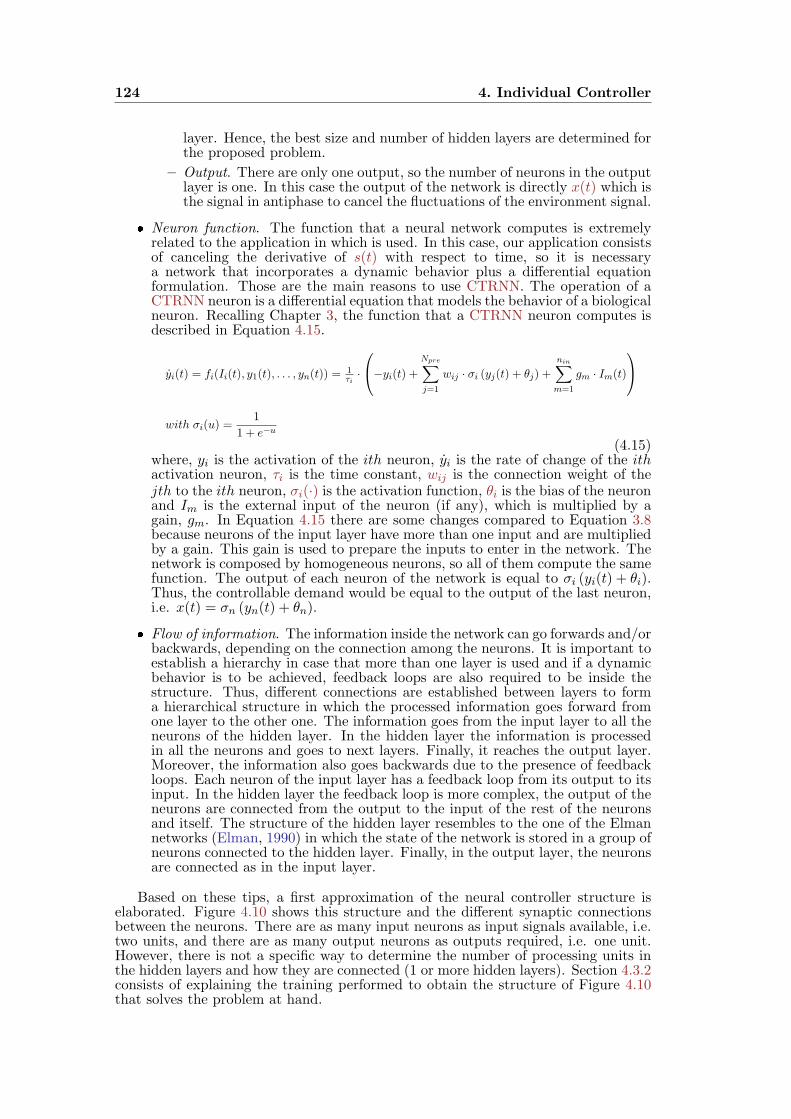
124 4. Individual Controller
layer. Hence, the best size and number of hidden layers are determined forthe proposed problem.
– Output. There are only one output, so the number of neurons in the outputlayer is one. In this case the output of the network is directly x(t) which isthe signal in antiphase to cancel the fluctuations of the environment signal.
Neuron function. The function that a neural network computes is extremelyrelated to the application in which is used. In this case, our application consistsof canceling the derivative of s(t) with respect to time, so it is necessarya network that incorporates a dynamic behavior plus a differential equationformulation. Those are the main reasons to use CTRNN. The operation of aCTRNN neuron is a differential equation that models the behavior of a biologicalneuron. Recalling Chapter 3, the function that a CTRNN neuron computes isdescribed in Equation 4.15.
yi(t) = fi(Ii(t), y1(t), . . . , yn(t)) =1τi·
−yi(t) + Npre∑j=1
wij · σi (yj(t) + θj) +
nin∑m=1
gm · Im(t)
with σi(u) =
1
1 + e−u
(4.15)where, yi is the activation of the ith neuron, yi is the rate of change of the ithactivation neuron, τi is the time constant, wij is the connection weight of thejth to the ith neuron, σi(·) is the activation function, θi is the bias of the neuronand Im is the external input of the neuron (if any), which is multiplied by again, gm. In Equation 4.15 there are some changes compared to Equation 3.8because neurons of the input layer have more than one input and are multipliedby a gain. This gain is used to prepare the inputs to enter in the network. Thenetwork is composed by homogeneous neurons, so all of them compute the samefunction. The output of each neuron of the network is equal to σi (yi(t) + θi).Thus, the controllable demand would be equal to the output of the last neuron,i.e. x(t) = σn (yn(t) + θn).
Flow of information. The information inside the network can go forwards and/orbackwards, depending on the connection among the neurons. It is important toestablish a hierarchy in case that more than one layer is used and if a dynamicbehavior is to be achieved, feedback loops are also required to be inside thestructure. Thus, different connections are established between layers to forma hierarchical structure in which the processed information goes forward fromone layer to the other one. The information goes from the input layer to all theneurons of the hidden layer. In the hidden layer the information is processedin all the neurons and goes to next layers. Finally, it reaches the output layer.Moreover, the information also goes backwards due to the presence of feedbackloops. Each neuron of the input layer has a feedback loop from its output to itsinput. In the hidden layer the feedback loop is more complex, the output of theneurons are connected from the output to the input of the rest of the neuronsand itself. The structure of the hidden layer resembles to the one of the Elmannetworks (Elman, 1990) in which the state of the network is stored in a group ofneurons connected to the hidden layer. Finally, in the output layer, the neuronsare connected as in the input layer.
Based on these tips, a first approximation of the neural controller structure iselaborated. Figure 4.10 shows this structure and the different synaptic connectionsbetween the neurons. There are as many input neurons as input signals available, i.e.two units, and there are as many output neurons as outputs required, i.e. one unit.However, there is not a specific way to determine the number of processing units inthe hidden layers and how they are connected (1 or more hidden layers). Section 4.3.2consists of explaining the training performed to obtain the structure of Figure 4.10that solves the problem at hand.
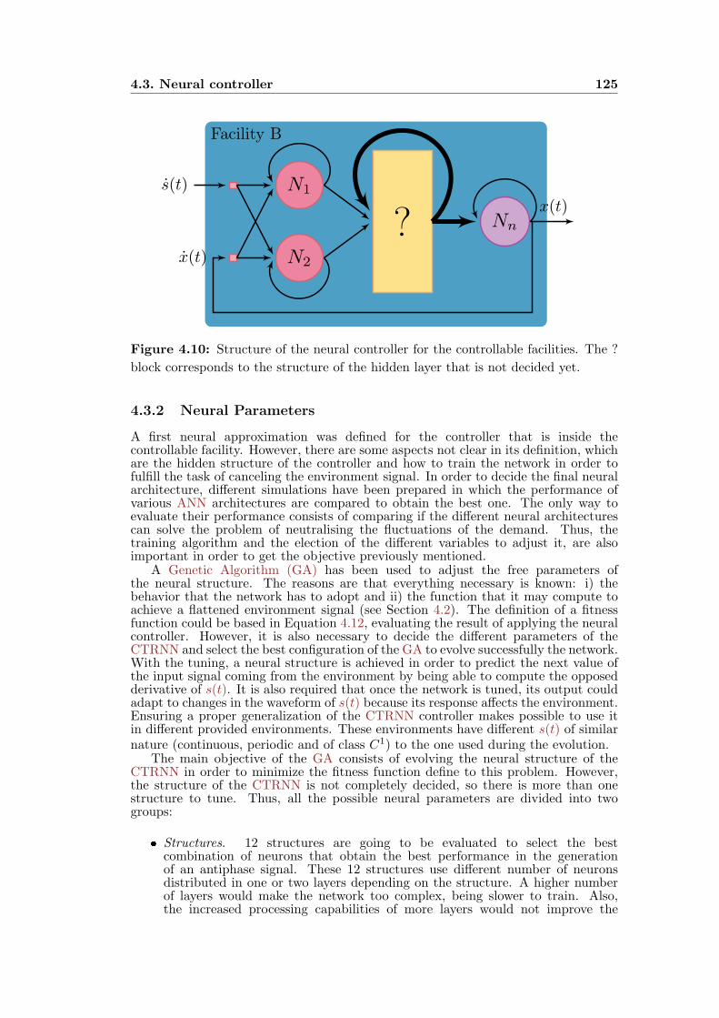
4.3. Neural controller 125
Facility B
N1
N2
? Nn
x(t)
x(t)
s(t)
Figure 4.10: Structure of the neural controller for the controllable facilities. The ?
block corresponds to the structure of the hidden layer that is not decided yet.
4.3.2 Neural Parameters
A first neural approximation was defined for the controller that is inside thecontrollable facility. However, there are some aspects not clear in its definition, whichare the hidden structure of the controller and how to train the network in order tofulfill the task of canceling the environment signal. In order to decide the final neuralarchitecture, different simulations have been prepared in which the performance ofvarious ANN architectures are compared to obtain the best one. The only way toevaluate their performance consists of comparing if the different neural architecturescan solve the problem of neutralising the fluctuations of the demand. Thus, thetraining algorithm and the election of the different variables to adjust it, are alsoimportant in order to get the objective previously mentioned.
A Genetic Algorithm (GA) has been used to adjust the free parameters ofthe neural structure. The reasons are that everything necessary is known: i) thebehavior that the network has to adopt and ii) the function that it may compute toachieve a flattened environment signal (see Section 4.2). The definition of a fitnessfunction could be based in Equation 4.12, evaluating the result of applying the neuralcontroller. However, it is also necessary to decide the different parameters of theCTRNN and select the best configuration of the GA to evolve successfully the network.With the tuning, a neural structure is achieved in order to predict the next value ofthe input signal coming from the environment by being able to compute the opposedderivative of s(t). It is also required that once the network is tuned, its output couldadapt to changes in the waveform of s(t) because its response affects the environment.Ensuring a proper generalization of the CTRNN controller makes possible to use itin different provided environments. These environments have different s(t) of similarnature (continuous, periodic and of class C1) to the one used during the evolution.
The main objective of the GA consists of evolving the neural structure of theCTRNN in order to minimize the fitness function define to this problem. However,the structure of the CTRNN is not completely decided, so there is more than onestructure to tune. Thus, all the possible neural parameters are divided into twogroups:
Structures. 12 structures are going to be evaluated to select the bestcombination of neurons that obtain the best performance in the generationof an antiphase signal. These 12 structures use different number of neuronsdistributed in one or two layers depending on the structure. A higher numberof layers would make the network too complex, being slower to train. Also,the increased processing capabilities of more layers would not improve the
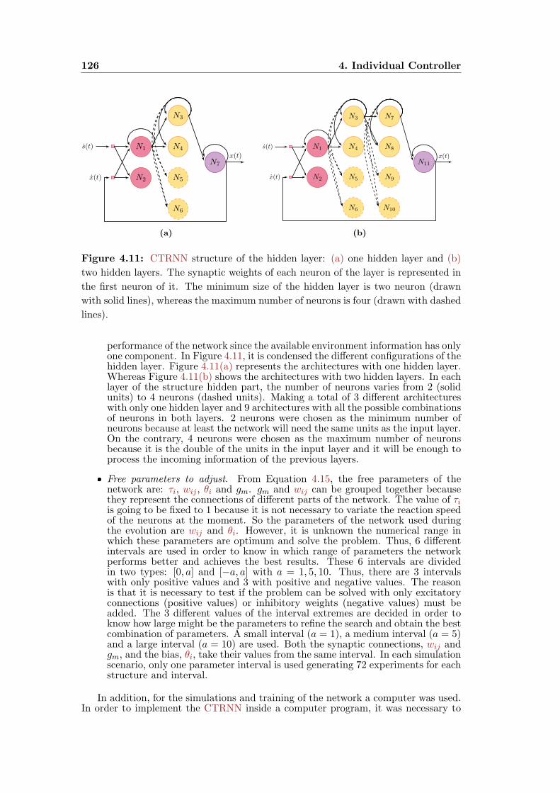
126 4. Individual Controller
N3
N1 N4
N2 N5
N6
N7
x(t)
x(t)
s(t)
(a)
N3 N7
N1 N4 N8
N2 N5 N9
N6 N10
N11
x(t)
x(t)
s(t)
(b)
Figure 4.11: CTRNN structure of the hidden layer: (a) one hidden layer and (b)
two hidden layers. The synaptic weights of each neuron of the layer is represented in
the first neuron of it. The minimum size of the hidden layer is two neuron (drawn
with solid lines), whereas the maximum number of neurons is four (drawn with dashed
lines).
performance of the network since the available environment information has onlyone component. In Figure 4.11, it is condensed the different configurations of thehidden layer. Figure 4.11(a) represents the architectures with one hidden layer.Whereas Figure 4.11(b) shows the architectures with two hidden layers. In eachlayer of the structure hidden part, the number of neurons varies from 2 (solidunits) to 4 neurons (dashed units). Making a total of 3 different architectureswith only one hidden layer and 9 architectures with all the possible combinationsof neurons in both layers. 2 neurons were chosen as the minimum number ofneurons because at least the network will need the same units as the input layer.On the contrary, 4 neurons were chosen as the maximum number of neuronsbecause it is the double of the units in the input layer and it will be enough toprocess the incoming information of the previous layers.
Free parameters to adjust. From Equation 4.15, the free parameters of thenetwork are: τi, wij , θi and gm. gm and wij can be grouped together becausethey represent the connections of different parts of the network. The value of τiis going to be fixed to 1 because it is not necessary to variate the reaction speedof the neurons at the moment. So the parameters of the network used duringthe evolution are wij and θi. However, it is unknown the numerical range inwhich these parameters are optimum and solve the problem. Thus, 6 differentintervals are used in order to know in which range of parameters the networkperforms better and achieves the best results. These 6 intervals are dividedin two types: [0, a] and [−a, a] with a = 1, 5, 10. Thus, there are 3 intervalswith only positive values and 3 with positive and negative values. The reasonis that it is necessary to test if the problem can be solved with only excitatoryconnections (positive values) or inhibitory weights (negative values) must beadded. The 3 different values of the interval extremes are decided in order toknow how large might be the parameters to refine the search and obtain the bestcombination of parameters. A small interval (a = 1), a medium interval (a = 5)and a large interval (a = 10) are used. Both the synaptic connections, wij andgm, and the bias, θi, take their values from the same interval. In each simulationscenario, only one parameter interval is used generating 72 experiments for eachstructure and interval.
In addition, for the simulations and training of the network a computer was used.In order to implement the CTRNN inside a computer program, it was necessary to
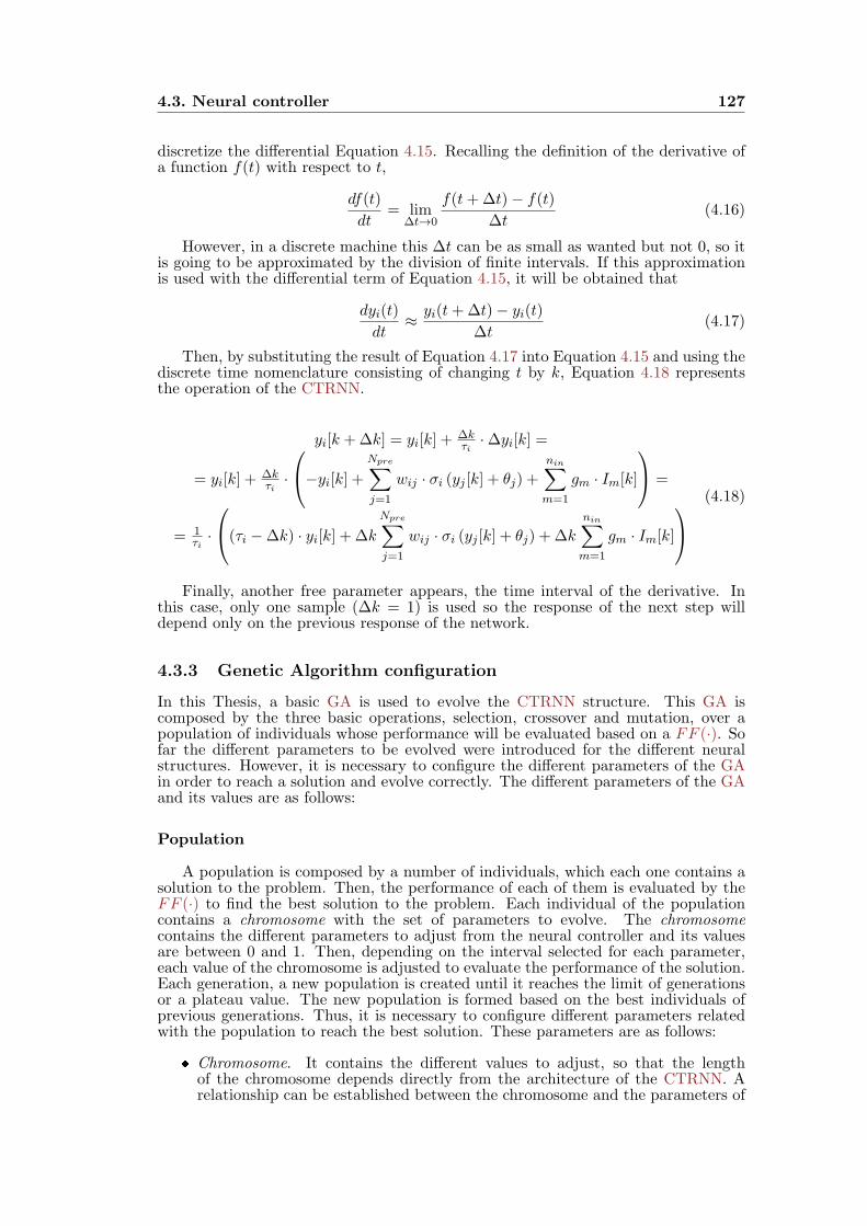
4.3. Neural controller 127
discretize the differential Equation 4.15. Recalling the definition of the derivative ofa function f(t) with respect to t,
df(t)
dt= lim
∆t→0
f(t+∆t)− f(t)
∆t(4.16)
However, in a discrete machine this ∆t can be as small as wanted but not 0, so itis going to be approximated by the division of finite intervals. If this approximationis used with the differential term of Equation 4.15, it will be obtained that
dyi(t)
dt≈ yi(t+∆t)− yi(t)
∆t(4.17)
Then, by substituting the result of Equation 4.17 into Equation 4.15 and using thediscrete time nomenclature consisting of changing t by k, Equation 4.18 representsthe operation of the CTRNN.
yi[k +∆k] = yi[k] +∆kτi·∆yi[k] =
= yi[k] +∆kτi·
−yi[k] + Npre∑j=1
wij · σi (yj [k] + θj) +
nin∑m=1
gm · Im[k]
=
= 1τi·
(τi −∆k) · yi[k] + ∆k
Npre∑j=1
wij · σi (yj [k] + θj) + ∆k
nin∑m=1
gm · Im[k]
(4.18)
Finally, another free parameter appears, the time interval of the derivative. Inthis case, only one sample (∆k = 1) is used so the response of the next step willdepend only on the previous response of the network.
4.3.3 Genetic Algorithm configuration
In this Thesis, a basic GA is used to evolve the CTRNN structure. This GA iscomposed by the three basic operations, selection, crossover and mutation, over apopulation of individuals whose performance will be evaluated based on a FF (·). Sofar the different parameters to be evolved were introduced for the different neuralstructures. However, it is necessary to configure the different parameters of the GAin order to reach a solution and evolve correctly. The different parameters of the GAand its values are as follows:
Population
A population is composed by a number of individuals, which each one contains asolution to the problem. Then, the performance of each of them is evaluated by theFF (·) to find the best solution to the problem. Each individual of the populationcontains a chromosome with the set of parameters to evolve. The chromosomecontains the different parameters to adjust from the neural controller and its valuesare between 0 and 1. Then, depending on the interval selected for each parameter,each value of the chromosome is adjusted to evaluate the performance of the solution.Each generation, a new population is created until it reaches the limit of generationsor a plateau value. The new population is formed based on the best individuals ofprevious generations. Thus, it is necessary to configure different parameters relatedwith the population to reach the best solution. These parameters are as follows:
Chromosome. It contains the different values to adjust, so that the lengthof the chromosome depends directly from the architecture of the CTRNN. Arelationship can be established between the chromosome and the parameters of

128 4. Individual Controller
the neural network. Thus, the chromosome is composed by the different wijand θi, which is expressed mathematically in Equation 4.19.
lch =
input︷ ︸︸ ︷Nin · (nin + 1)+
hidden︷ ︸︸ ︷L∑l=1
Nh,l · (Npl,l +Nh,l)+
output︷ ︸︸ ︷No · (Npl + 1)+
bias︷︸︸︷NT (4.19)
where, lch is the length of the chromosome, Nin is the number of neurons in theinput layer, nin is the number of inputs associated with the gm terms, Nh,l isthe number of neurons of the lth hidden layer, Npl,l is the number of neuronsof the previous layer, No is the number of neurons in the output layer and NTis the total number of neurons. Over each term of Equation 4.19 is the nameof the part of the neural structure to which corresponds. The minimum lengthof the chromosome corresponds to the neural architecture with only 1 hiddenlayer and 2 neurons in it, and it has a value of 22 genes. Whereas the maximumlength corresponds to the structure with 2 hidden layers and 4 neurons in eachof them, that is 78 genes. The length of the rest of structures is between 22 and78 genes, so it is also necessary to adjust correctly the parameters of the GA tofind the best solution in each case.
Size. The population size affects the speed to find the solution. The higher thesize of the population is, the greater the number of solutions are tried. So, thereare more possibilities to find the best solution for big populations. During thetuning process, different population sizes are tested to find the optimum numberof individuals per generation. The size of the populations varies between 20to 100 individuals with intervals of 10 individuals of difference between them.Thus, 9 different populations sizes are tested.
Generations. It is also required that evolution is limited in order to finishrunning the GA. In first place, the number of generations should be high enoughso that the algorithm can reach the solution within it. On the other hand, thisnumber guarantees that the simulation stops in a hard limit. In case that it isa large number, it would take a long time for simulating it when any optimalsolution is not reached. For these simulations, this number was fixed to 1000generations because it is enough to prove the validity of the CTRNN under theparameters found.
Selection
This is one of the genetic operators that builds the next generation of individuals.It is based on the mechanism described in Section 3.5.2.2. The one selected is theroulette-wheel method. This operator consists of reordering the individuals based ontheir fitness value. The bigger the fitness value is, the bigger chances the individualhas to be selected. Then, a number of individuals are selected randomly based ontheir probability. The number of selections is based on the population size. However,based only on the randomness of the process, diversity and the best fitted solutionof the problem can be lost. To solve this problem, a combination of the roulette-wheel method with the elitism is selected. Thus, a number of individuals of the nextgeneration is reserved to copy directly which consists of the best individuals of theprevious generation. In this case, the number of elites is fixed to 6, being enough tobreed the next generation.
Crossover
The crossover operator is applied over the individuals obtained from the previousselection. This operator consists of creating a new offspring from the selectedindividuals of the previous generation that would breed new individuals in the nextgeneration. The idea of the operator is to choose two individuals, select randomly a

4.3. Neural controller 129
point in their chromosomes and then swap the parts of the chromosomes. Therefore,two individuals are created for the new generation with part of their predecessors. Thecrossover favors the exploration of the search scenario. There are different crossoveroperators, but the simplest one was used to make the GA quick and to prove thatthe network can be trained with the simplest algorithm. The crossover operator onlyselects 1 point to cross the chromosome. This point is randomly chosen among thedifferent genes of the chromosome.
Mutation
This is the last genetic operator implemented. It consists of changing the value ofa gene inside the chromosome randomly with a very low probability. In this case thevalue of the gene is altered following a Normal Gaussian distribution with a varianceof σ = 0.2, whose value will be added to the gene in order to modify its value. Thisoperator is used due to the introduction of diversity inside the population. It alsohelps to avoid favoring one individual against others in the genetic drift, to avoidthe premature convergence of the algorithm and to guarantee that the algorithm willfound the global solution with enough time. Different mutation rates are used inorder to find the best one for the problem. These rates are between 0.01 and 0.1 insteps of 0.01. So, there are 10 different mutation rates to select the best choice forour algorithm.
Fitness function
The last element of the GA configuration is the evaluation of the individuals.FF (·) is in charge of evaluating the performance of the different chromosomes oncethey have been used for its purpose inside the simulation as the parameters of theCTRNN. The form of this function is defined by the user, but it should contain theelements needed to minimize the objective of the neural structure selected. In thiscase, a function is built to be capable of evaluating the capacity of the correspondingCTRNN structure to be in antiphase to the C1 input signal. In Section 4.2, it wasconcluded that a controllable user has to behave as Equation 4.12 to get an antiphasesignal. Hence, based on Equation 4.12, a first approximation of the FF (·) is as follows(see Figure 4.12(a)).
FFi (s(t)) =
1; if s(t) = 0
0; otherwise(4.20)
where FFi (s(t)) is the fitness value of an individual. However, a GA does not behavewell with discontinuous fitness functions like the one formulated in Equation 4.20.The reason is that it seems like only the individuals that reach the condition have afitness value, the rest are equal to 0. So, imagine that neither of the individuals geta value different from 0, the GA could not evolve because none of the solutions hasa fitness value. That is to say, a GA with such a FF (·) would not converge to anappropriate solution to the problem.
Thus, it is necessary to change the abrupt formulation of Equation 4.20 in orderto make the algorithm converge to the solution. To do that, the condition of theFFi (s(t)) is relaxed and a gradual transition is made between the two states (seeFigure 4.12(b)). With the relaxation of the condition, more individuals can scoreand evolve to better solutions in order to reach the maximum fitness. Equation 4.21shows a gradual fitness function formulation of Equation 4.20.
FFi (s(t)) =
1; if |s(t)| < ε
−|s(t)| − δ
δ − ε; if ε ≤ |s(t)| ≤ δ
0; if |s(t)| > δ
(4.21)
where, ε is the inferior limit and δ is the superior limit. Being ε << δ. In Equation4.21, the direction of the derivative is not taken into account because the algorithm
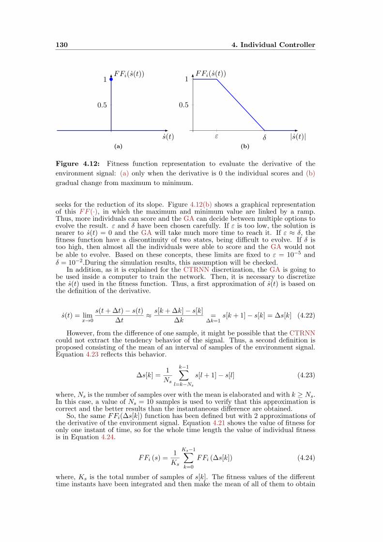
130 4. Individual Controller
0.5
1
s(t)
FFi(s(t))
(a)
0.5
1
ε δ |s(t)|
FFi(s(t))
(b)
Figure 4.12: Fitness function representation to evaluate the derivative of the
environment signal: (a) only when the derivative is 0 the individual scores and (b)
gradual change from maximum to minimum.
seeks for the reduction of its slope. Figure 4.12(b) shows a graphical representationof this FF (·), in which the maximum and minimum value are linked by a ramp.Thus, more individuals can score and the GA can decide between multiple options toevolve the result. ε and δ have been chosen carefully. If ε is too low, the solution isnearer to s(t) = 0 and the GA will take much more time to reach it. If ε ≈ δ, thefitness function have a discontinuity of two states, being difficult to evolve. If δ istoo high, then almost all the individuals were able to score and the GA would notbe able to evolve. Based on these concepts, these limits are fixed to ε = 10−5 andδ = 10−2.During the simulation results, this assumption will be checked.
In addition, as it is explained for the CTRNN discretization, the GA is going tobe used inside a computer to train the network. Then, it is necessary to discretizethe s(t) used in the fitness function. Thus, a first approximation of s(t) is based onthe definition of the derivative.
s(t) = limx→0
s(t+∆t)− s(t)
∆t≈ s[k +∆k]− s[k]
∆k=
∆k=1s[k + 1]− s[k] = ∆s[k] (4.22)
However, from the difference of one sample, it might be possible that the CTRNNcould not extract the tendency behavior of the signal. Thus, a second definition isproposed consisting of the mean of an interval of samples of the environment signal.Equation 4.23 reflects this behavior.
∆s[k] =1
Ns
k−1∑l=k−Ns
s[l + 1]− s[l] (4.23)
where, Ns is the number of samples over with the mean is elaborated and with k ≥ Ns.In this case, a value of Ns = 10 samples is used to verify that this approximation iscorrect and the better results than the instantaneous difference are obtained.
So, the same FFi(∆s[k]) function has been defined but with 2 approximations ofthe derivative of the environment signal. Equation 4.21 shows the value of fitness foronly one instant of time, so for the whole time length the value of individual fitnessis in Equation 4.24.
FFi (s) =1
Ks
Ks−1∑k=0
FFi (∆s[k]) (4.24)
where, Ks is the total number of samples of s[k]. The fitness values of the differenttime instants have been integrated and then make the mean of all of them to obtain
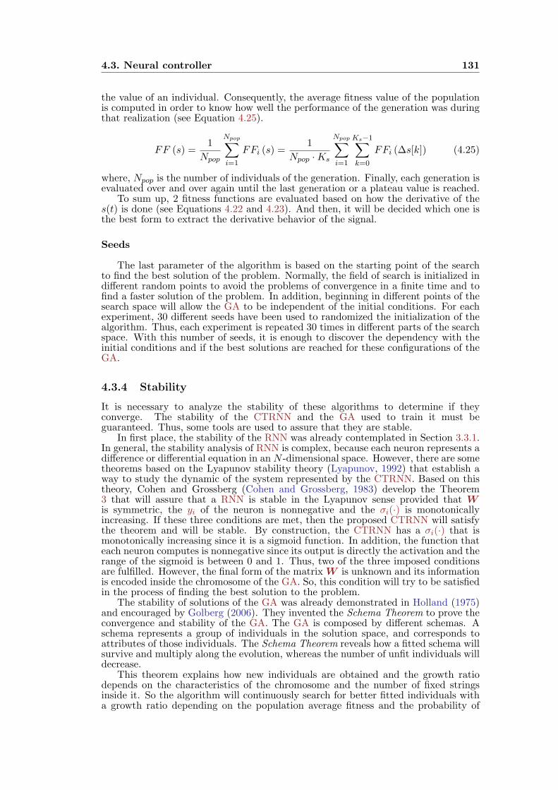
4.3. Neural controller 131
the value of an individual. Consequently, the average fitness value of the populationis computed in order to know how well the performance of the generation was duringthat realization (see Equation 4.25).
FF (s) =1
Npop
Npop∑i=1
FFi (s) =1
Npop ·Ks
Npop∑i=1
Ks−1∑k=0
FFi (∆s[k]) (4.25)
where, Npop is the number of individuals of the generation. Finally, each generation isevaluated over and over again until the last generation or a plateau value is reached.
To sum up, 2 fitness functions are evaluated based on how the derivative of thes(t) is done (see Equations 4.22 and 4.23). And then, it will be decided which one isthe best form to extract the derivative behavior of the signal.
Seeds
The last parameter of the algorithm is based on the starting point of the searchto find the best solution of the problem. Normally, the field of search is initialized indifferent random points to avoid the problems of convergence in a finite time and tofind a faster solution of the problem. In addition, beginning in different points of thesearch space will allow the GA to be independent of the initial conditions. For eachexperiment, 30 different seeds have been used to randomized the initialization of thealgorithm. Thus, each experiment is repeated 30 times in different parts of the searchspace. With this number of seeds, it is enough to discover the dependency with theinitial conditions and if the best solutions are reached for these configurations of theGA.
4.3.4 Stability
It is necessary to analyze the stability of these algorithms to determine if theyconverge. The stability of the CTRNN and the GA used to train it must beguaranteed. Thus, some tools are used to assure that they are stable.
In first place, the stability of the RNN was already contemplated in Section 3.3.1.In general, the stability analysis of RNN is complex, because each neuron represents adifference or differential equation in an N -dimensional space. However, there are sometheorems based on the Lyapunov stability theory (Lyapunov, 1992) that establish away to study the dynamic of the system represented by the CTRNN. Based on thistheory, Cohen and Grossberg (Cohen and Grossberg, 1983) develop the Theorem3 that will assure that a RNN is stable in the Lyapunov sense provided that Wis symmetric, the yi of the neuron is nonnegative and the σi(·) is monotonicallyincreasing. If these three conditions are met, then the proposed CTRNN will satisfythe theorem and will be stable. By construction, the CTRNN has a σi(·) that ismonotonically increasing since it is a sigmoid function. In addition, the function thateach neuron computes is nonnegative since its output is directly the activation and therange of the sigmoid is between 0 and 1. Thus, two of the three imposed conditionsare fulfilled. However, the final form of the matrix W is unknown and its informationis encoded inside the chromosome of the GA. So, this condition will try to be satisfiedin the process of finding the best solution to the problem.
The stability of solutions of the GA was already demonstrated in Holland (1975)and encouraged by Golberg (2006). They invented the Schema Theorem to prove theconvergence and stability of the GA. The GA is composed by different schemas. Aschema represents a group of individuals in the solution space, and corresponds toattributes of those individuals. The Schema Theorem reveals how a fitted schema willsurvive and multiply along the evolution, whereas the number of unfit individuals willdecrease.
This theorem explains how new individuals are obtained and the growth ratiodepends on the characteristics of the chromosome and the number of fixed stringsinside it. So the algorithm will continuously search for better fitted individuals witha growth ratio depending on the population average fitness and the probability of

132 4. Individual Controller
ANN Parameters min max
W and gm 17 67
θi 5 11
τi – 1
# hidden layers 1 2
# hidden neurons 2 4
Total # of neurons 5 11
Total # structures 12
Total # intervals 6
Table 4.1: Configuration of the ANN for
the different simulations.
GA Parameters min max
chromosome length 22 78
Population size 20 100
# generations – 1000
# elites – 6
# crossovers – 1
Mutation rate 0.01 0.1
# FF (·) – 2
# seeds – 30
Table 4.2: Configuration of the GA for
the different simulations.
surviving the operations. To sum up, both of the algorithms used (CTRNN and GA)are built following both theorems (Cohen-Grossberg Theorem and Schema Theorem)so that they provided the necessary conditions to assure the stability of the algorithms.
4.4 Simulation Results
At the end of the training for all the different simulation configurations, the bestCTRNN architecture and the best parameters of the GA will be obtained. FromSections 4.3.2 and 4.3.3, the different parameters of the simulations are reduced toTables 4.1 and 4.2. Thus, there are 12 different CTRNN structures which use 6different intervals for their free parameters and they are trained with a GA thathas 9 different sizes of populations evolved in 1000 generations with the 3 basicgenetic operators: selection with 6 elites, 1 crossover and 10 different mutationsrates, evaluated for 2 fitness functions. And each experiment is repeated 30 timesto randomize the initial conditions of the algorithm. So the number of simulations tobe done is 388800 in total.
All the simulations under the set of parameters of Tables 4.1 and 4.2 are conductedby NeuralSim simulator. NeuralSim is an open source simulator under GPLv3.0license developed in C++. It was build as a general purpose simulator to provedifferent neural structures with different methods to train them, learning algorithmsand GAs. The simulator is built following a modular structure so anyone can configuredifferent neural structures with different neural functions. The different parametersof the neural network and the algorithm used to train it, are configured throughdifferent XML files. All the simulations were run in a computing cluster of 60 unitprocessors of AMD Opteron(tm) Processor 4180 with 40GB of RAM memory, undera distribution Rocks 6.1.1 (Sand Boa) of 64 bits architecture.
Before presenting the simulation results, it is needed to talked about the inputsignal of the neural controller. Its aim is to smooth the aggregated consumption of agrid, but a more general input signal is used for this preliminary study to determinethe best configuration of the CTRNN and the GA. Thus, a continuous periodic signalof class C1 is required to evaluate the neural structure and check if the derivativeintuition to smooth a curve is correct. In this case, a sinusoidal function is usedwhich possesses all characteristics and similar properties of the one to smooth. Inaddition, it is also necessary a representative waveform of the varying consumptionwith its peaks and valleys. Therefore, a sinusoid is used with a day period to simulatea peak and a valley. However, a high resolution sinusoid is not used with 1440 samplesper period as it length in minutes of a day. The idea is to use a sampled sinusoidalof 72 samples per period so that it is the same as sampling the daily aggregatedconsumption every 20minutes. Moreover, the input signal is formed of 3 periods of
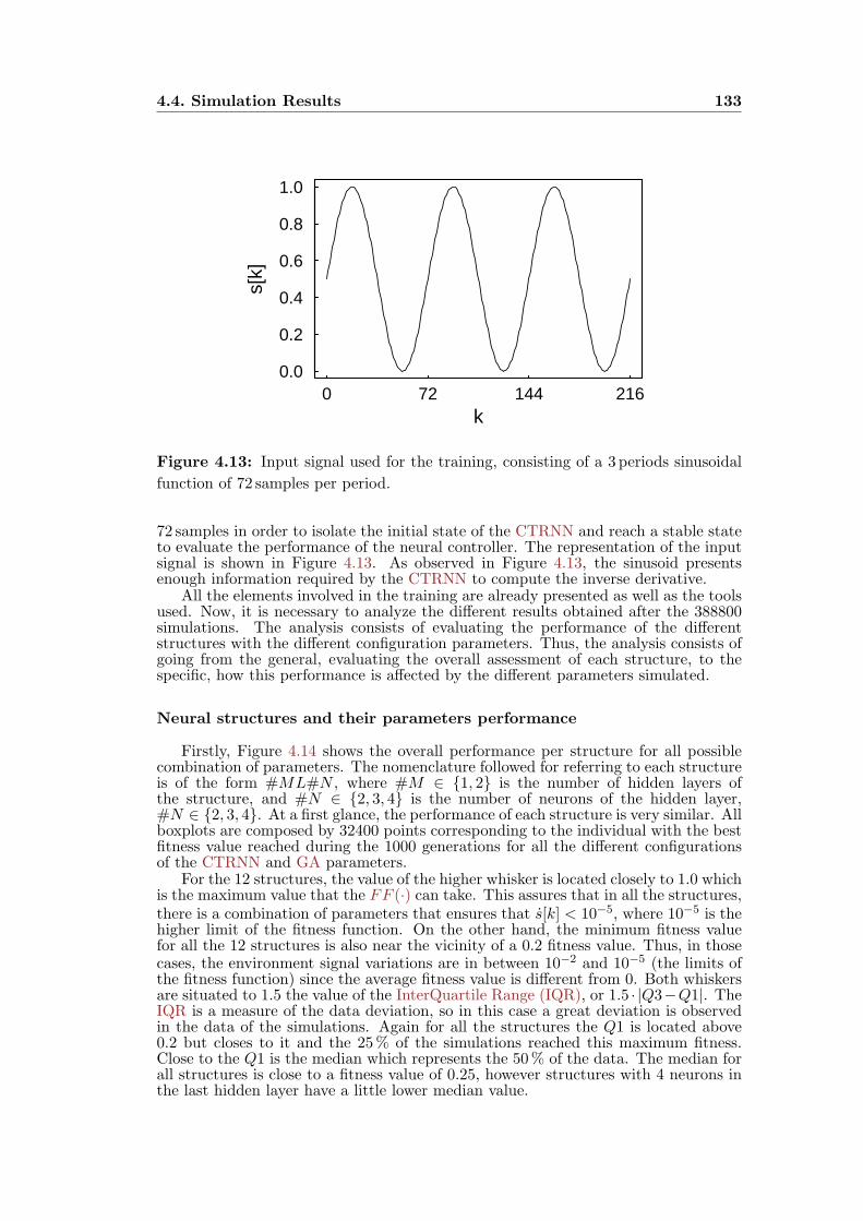
4.4. Simulation Results 133
0 72 144 2160.0
0.2
0.4
0.6
0.8
1.0
k
s[k]
Figure 4.13: Input signal used for the training, consisting of a 3 periods sinusoidal
function of 72 samples per period.
72 samples in order to isolate the initial state of the CTRNN and reach a stable stateto evaluate the performance of the neural controller. The representation of the inputsignal is shown in Figure 4.13. As observed in Figure 4.13, the sinusoid presentsenough information required by the CTRNN to compute the inverse derivative.
All the elements involved in the training are already presented as well as the toolsused. Now, it is necessary to analyze the different results obtained after the 388800simulations. The analysis consists of evaluating the performance of the differentstructures with the different configuration parameters. Thus, the analysis consists ofgoing from the general, evaluating the overall assessment of each structure, to thespecific, how this performance is affected by the different parameters simulated.
Neural structures and their parameters performance
Firstly, Figure 4.14 shows the overall performance per structure for all possiblecombination of parameters. The nomenclature followed for referring to each structureis of the form #ML#N , where #M ∈ 1, 2 is the number of hidden layers ofthe structure, and #N ∈ 2, 3, 4 is the number of neurons of the hidden layer,#N ∈ 2, 3, 4. At a first glance, the performance of each structure is very similar. Allboxplots are composed by 32400 points corresponding to the individual with the bestfitness value reached during the 1000 generations for all the different configurationsof the CTRNN and GA parameters.
For the 12 structures, the value of the higher whisker is located closely to 1.0 whichis the maximum value that the FF (·) can take. This assures that in all the structures,there is a combination of parameters that ensures that s[k] < 10−5, where 10−5 is thehigher limit of the fitness function. On the other hand, the minimum fitness valuefor all the 12 structures is also near the vicinity of a 0.2 fitness value. Thus, in thosecases, the environment signal variations are in between 10−2 and 10−5 (the limits ofthe fitness function) since the average fitness value is different from 0. Both whiskersare situated to 1.5 the value of the InterQuartile Range (IQR), or 1.5 · |Q3−Q1|. TheIQR is a measure of the data deviation, so in this case a great deviation is observedin the data of the simulations. Again for all the structures the Q1 is located above0.2 but closes to it and the 25% of the simulations reached this maximum fitness.Close to the Q1 is the median which represents the 50% of the data. The median forall structures is close to a fitness value of 0.25, however structures with 4 neurons inthe last hidden layer have a little lower median value.

134 4. Individual Controller
0.2
0.4
0.6
0.8
1.0
1L2 1L3 1L4 2L22 2L23 2L24 2L32 2L33 2L34 2L42 2L43 2L44Structure
Fitn
ess
Figure 4.14: Overall fitness performance per structure for all the possible
configurations of the simulations. The nomenclature of the structure is #ML#N
with #M , the number of hidden layers, and #N , the number of hidden neurons.
Each box comprises observations ranging from the first to the third quartile. The
median is indicated by a horizontal bar, dividing the box into the upper and lower
part. The whiskers extend to the farthest data points that are within 1.5 times the
interquartile range. Outliers are shown as dots.
Finally, the Q3 for all the simulations is above a 0.8 fitness value, so that the25% of the simulations are above this value. Thus, for these 25% of simulations, it iscloser to the higher limit of the fitness function and the amplitude of the variationsof s[k] are almost reduced. In addition, it can be observed, some differences betweenthe values of Q3 depending on the structure. The best value of the Q3 correspondsto the structure 1L4 (1 hidden layer with 4 neurons), but in general the performanceof the architectures with only one hidden layer are only 1% above the two layersarchitectures. This figure seems relatively too low to state which structure is thebest. However, it can be concluded that the complexity introduced by the two hiddenlayers do not achieve better results than the ones with a hidden layer. The tuningis reduced since fewer parameters are used and the processing capabilities are morefitted to requirements of the problem.
Nevertheless, the information of Figure 4.14 is not enough to reach any conclusion.So, the data corresponding to each structure are split in the different ranges of thetuple W ,Θ. Figure 4.15 shows all the results for the different ranges of valuesthat the parameters of the CTRNN can take. In order to reduce the volume ofdata, the seeds of the different configurations have been grouped to analyze the meanperformance of each evolution since all the structures behave similarly. A first divisionhas been made based on the form of the value ranges. The two ranges selected are: i)[0, a], only positive values, and ii) [−a, a], symmetric range of values. The first rangeindicates that there is no inhibition inside the neurons, so the connections and biaswill excite the next response coming from the previous neurons. On the contrary,the range of values of the form [−a, a] allow neurons to have excitatory or inhibitoryconnections which increase the adaptivity and the regulation of the neural activation.These assumptions are also corroborated by the results shown in Figure 4.15(a).
For all the structures, when W ,Θ ∈ [0, a] there is no difference in the fitnessvalue for each one. In all these cases, the structure is far from reaching the maximumvalue of the fitness, so hardly these structures are evolved. This behavior occursdue to the absence of inhibitory synapses. The neurons are saturated due to the
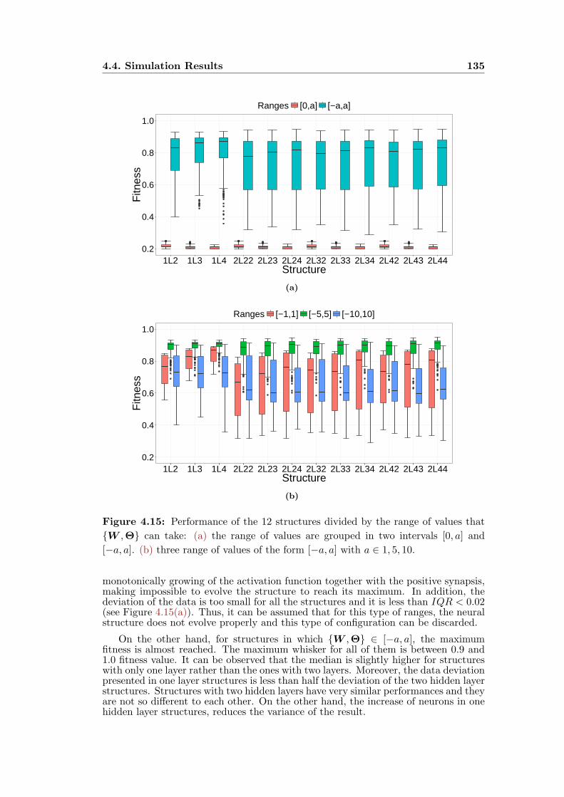
4.4. Simulation Results 135
0.2
0.4
0.6
0.8
1.0
1L2 1L3 1L4 2L22 2L23 2L24 2L32 2L33 2L34 2L42 2L43 2L44Structure
Fitn
ess
Ranges [0,a] [−a,a]
(a)
0.2
0.4
0.6
0.8
1.0
1L2 1L3 1L4 2L22 2L23 2L24 2L32 2L33 2L34 2L42 2L43 2L44Structure
Fitn
ess
Ranges [−1,1] [−5,5] [−10,10]
(b)
Figure 4.15: Performance of the 12 structures divided by the range of values that
W ,Θ can take: (a) the range of values are grouped in two intervals [0, a] and
[−a, a]. (b) three range of values of the form [−a, a] with a ∈ 1, 5, 10.
monotonically growing of the activation function together with the positive synapsis,making impossible to evolve the structure to reach its maximum. In addition, thedeviation of the data is too small for all the structures and it is less than IQR < 0.02(see Figure 4.15(a)). Thus, it can be assumed that for this type of ranges, the neuralstructure does not evolve properly and this type of configuration can be discarded.
On the other hand, for structures in which W ,Θ ∈ [−a, a], the maximumfitness is almost reached. The maximum whisker for all of them is between 0.9 and1.0 fitness value. It can be observed that the median is slightly higher for structureswith only one layer rather than the ones with two layers. Moreover, the data deviationpresented in one layer structures is less than half the deviation of the two hidden layerstructures. Structures with two hidden layers have very similar performances and theyare not so different to each other. On the other hand, the increase of neurons in onehidden layer structures, reduces the variance of the result.
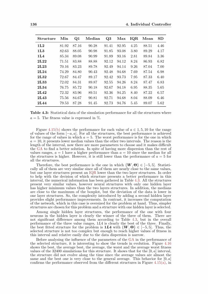
136 4. Individual Controller
Structure Min Q1 Median Q3 Max IQR Mean SD
1L2 81.92 87.16 90.28 91.41 92.95 4.25 88.51 4.46
1L3 82.63 88.05 90.98 91.85 93.08 3.80 89.29 4.17
1L4 85.34 89.08 90.99 91.89 93.16 2.81 89.84 3.36
2L22 71.51 83.88 88.88 92.12 94.12 8.24 86.93 6.82
2L23 70.16 83.23 89.78 92.49 94.14 9.26 87.04 7.00
2L24 74.29 84.80 90.43 92.48 94.68 7.69 87.54 6.98
2L32 72.67 84.47 89.17 92.42 93.73 7.95 87.33 6.40
2L33 72.02 84.31 89.87 92.55 94.26 8.24 87.47 6.83
2L34 76.75 85.72 90.18 92.67 94.18 6.95 88.35 5.65
2L42 72.32 83.96 89.51 92.36 94.25 8.40 87.22 6.57
2L43 75.56 84.67 90.81 92.71 94.68 8.04 88.09 6.46
2L44 79.53 87.28 91.45 92.73 94.76 5.45 89.07 5.62
Table 4.3: Statistical data of the simulation performance for all the structures where
a = 5. The fitness value is expressed in %.
Figure 4.15(b) shows the performance for each value of a ∈ 1, 5, 10 for the rangeof values of the form [−a, a]. For all the structures, the best performance is achievedfor the range of values in which a = 5. The worst performance is for the one in whicha = 10, it presents lower median values than the other two intervals. The reason is thelength of the interval, now there are more parameters to choose and it makes difficultthe GA to find a better solution. In spite of having more dispersion than the rest ofvalues ranges, a = 1 have a higher performance than a = 10 since the median for allthe structures is higher. However, it is still lower than the performance of a = 5 forall the structures.
Therefore, the best performance is the one in which W ,Θ ∈ [−5, 5]. Statisti-cally all of them are very similar since all of them are nearly close to the same values,but one layer structures present an IQR lower than the two layer structures. In orderto help with the decision of which structure presents a better performance in thisinterval, the numerical information has been gathered in Table 4.3. All the structurespresent very similar values, however neural structures with only one hidden layerhas higher minimum values than the two layers structures. In addition, the mediansare close to the maximum of the boxplot, but the deviation of the data is lower inone layer structures. So, the complexity introduced by adding a second hidden layerprovides slight performance improvements. In contrast, it increases the computationof the network, which in this case is oversized for the problem at hand. Thus, simplerstructures are chosen for this problem and a structure with one hidden layer is selected.
Among single hidden layer structures, the performance of the one with fourneurons in the hidden layer is clearly the winner of the three of them. There arenot significant difference among them according to Table 4.3, but in the overallperformance of the three value ranges, 1L4 is clearly the best of the three. Finally,the best fitted structure for the problem is 1L4 with W ,Θ ∈ [−5, 5]. Thus, theselected structure is not too complex but enough to reach higher values of fitness inthis interval and relative easily due to the data dispersion is narrow.
Before analysing the influence of the parameters of the GA in the performance ofthe selected structure, it is interesting to show the trends in evolution. Figure 4.16shows the best, the average best, the average, the worst and the average worst fitnessvalues of the 32400 simulations for this structure. It shows that for the [0, a] interval,the structure did not evolve along the time since the average values are almost thesame and the best one is very close to the general average. This behavior for [0, a]confirms the performance observed from the different structures in Figure 4.15(a), in
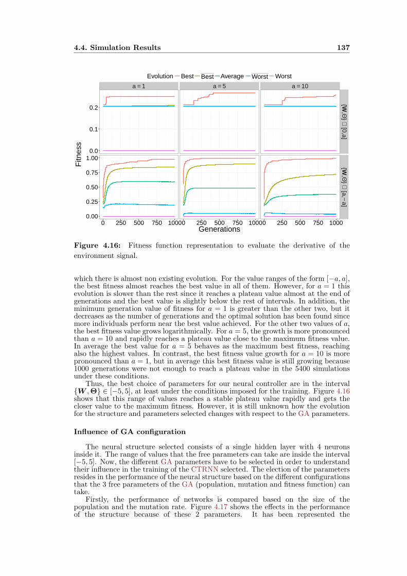
4.4. Simulation Results 137
a = 1 a = 5 a = 10
0.0
0.1
0.2
0.00
0.25
0.50
0.75
1.00
W,Θ
∈[0,a]
W,Θ
∈[a,−
a]
0 250 500 750 10000 250 500 750 10000 250 500 750 1000Generations
Fitn
ess
Evolution Best Best Average Worst Worst
Figure 4.16: Fitness function representation to evaluate the derivative of the
environment signal.
which there is almost non existing evolution. For the value ranges of the form [−a, a],the best fitness almost reaches the best value in all of them. However, for a = 1 thisevolution is slower than the rest since it reaches a plateau value almost at the end ofgenerations and the best value is slightly below the rest of intervals. In addition, theminimum generation value of fitness for a = 1 is greater than the other two, but itdecreases as the number of generations and the optimal solution has been found sincemore individuals perform near the best value achieved. For the other two values of a,the best fitness value grows logarithmically. For a = 5, the growth is more pronouncedthan a = 10 and rapidly reaches a plateau value close to the maximum fitness value.In average the best value for a = 5 behaves as the maximum best fitness, reachingalso the highest values. In contrast, the best fitness value growth for a = 10 is morepronounced than a = 1, but in average this best fitness value is still growing because1000 generations were not enough to reach a plateau value in the 5400 simulationsunder these conditions.
Thus, the best choice of parameters for our neural controller are in the intervalW ,Θ ∈ [−5, 5], at least under the conditions imposed for the training. Figure 4.16shows that this range of values reaches a stable plateau value rapidly and gets thecloser value to the maximum fitness. However, it is still unknown how the evolutionfor the structure and parameters selected changes with respect to the GA parameters.
Influence of GA configuration
The neural structure selected consists of a single hidden layer with 4 neuronsinside it. The range of values that the free parameters can take are inside the interval[−5, 5]. Now, the different GA parameters have to be selected in order to understandtheir influence in the training of the CTRNN selected. The election of the parametersresides in the performance of the neural structure based on the different configurationsthat the 3 free parameters of the GA (population, mutation and fitness function) cantake.
Firstly, the performance of networks is compared based on the size of thepopulation and the mutation rate. Figure 4.17 shows the effects in the performanceof the structure because of these 2 parameters. It has been represented the
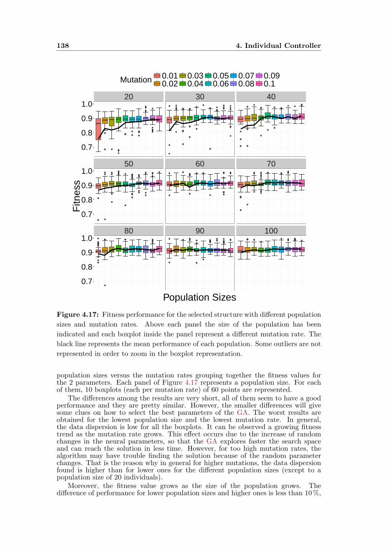
138 4. Individual Controller
20 30 40
50 60 70
80 90 100
0.7
0.8
0.9
1.0
0.7
0.8
0.9
1.0
0.7
0.8
0.9
1.0
Population Sizes
Fitn
ess
Mutation 0.010.02
0.030.04
0.050.06
0.070.08
0.090.1
Figure 4.17: Fitness performance for the selected structure with different population
sizes and mutation rates. Above each panel the size of the population has been
indicated and each boxplot inside the panel represent a different mutation rate. The
black line represents the mean performance of each population. Some outliers are not
represented in order to zoom in the boxplot representation.
population sizes versus the mutation rates grouping together the fitness values forthe 2 parameters. Each panel of Figure 4.17 represents a population size. For eachof them, 10 boxplots (each per mutation rate) of 60 points are represented.
The differences among the results are very short, all of them seem to have a goodperformance and they are pretty similar. However, the smaller differences will givesome clues on how to select the best parameters of the GA. The worst results areobtained for the lowest population size and the lowest mutation rate. In general,the data dispersion is low for all the boxplots. It can be observed a growing fitnesstrend as the mutation rate grows. This effect occurs due to the increase of randomchanges in the neural parameters, so that the GA explores faster the search spaceand can reach the solution in less time. However, for too high mutation rates, thealgorithm may have trouble finding the solution because of the random parameterchanges. That is the reason why in general for higher mutations, the data dispersionfound is higher than for lower ones for the different population sizes (except to apopulation size of 20 individuals).
Moreover, the fitness value grows as the size of the population grows. Thedifference of performance for lower population sizes and higher ones is less than 10%,
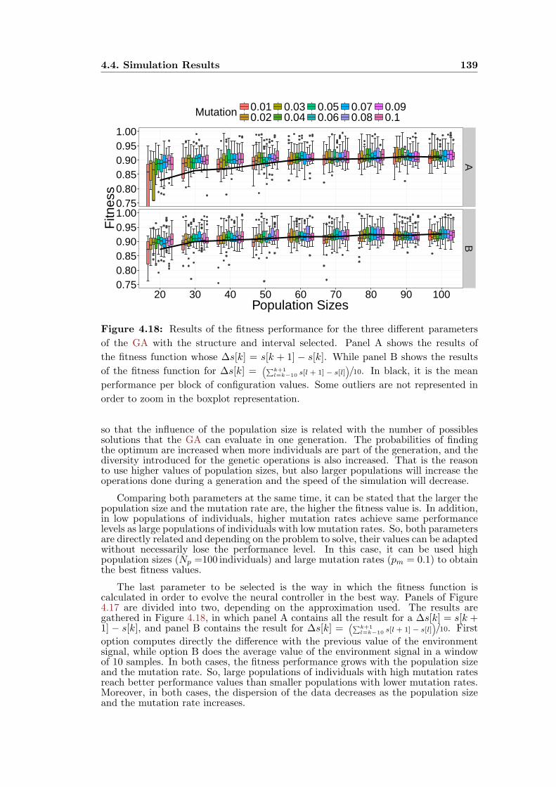
4.4. Simulation Results 139
0.750.800.850.900.951.00
0.750.800.850.900.951.00
AB
20 30 40 50 60 70 80 90 100Population Sizes
Fitn
ess
Mutation 0.010.02
0.030.04
0.050.06
0.070.08
0.090.1
Figure 4.18: Results of the fitness performance for the three different parameters
of the GA with the structure and interval selected. Panel A shows the results of
the fitness function whose ∆s[k] = s[k + 1] − s[k]. While panel B shows the results
of the fitness function for ∆s[k] =(∑k+1
l=k−10 s[l + 1] − s[l])/10. In black, it is the mean
performance per block of configuration values. Some outliers are not represented in
order to zoom in the boxplot representation.
so that the influence of the population size is related with the number of possiblessolutions that the GA can evaluate in one generation. The probabilities of findingthe optimum are increased when more individuals are part of the generation, and thediversity introduced for the genetic operations is also increased. That is the reasonto use higher values of population sizes, but also larger populations will increase theoperations done during a generation and the speed of the simulation will decrease.
Comparing both parameters at the same time, it can be stated that the larger thepopulation size and the mutation rate are, the higher the fitness value is. In addition,in low populations of individuals, higher mutation rates achieve same performancelevels as large populations of individuals with low mutation rates. So, both parametersare directly related and depending on the problem to solve, their values can be adaptedwithout necessarily lose the performance level. In this case, it can be used highpopulation sizes (Np =100 individuals) and large mutation rates (pm = 0.1) to obtainthe best fitness values.
The last parameter to be selected is the way in which the fitness function iscalculated in order to evolve the neural controller in the best way. Panels of Figure4.17 are divided into two, depending on the approximation used. The results aregathered in Figure 4.18, in which panel A contains all the result for a ∆s[k] = s[k +1] − s[k], and panel B contains the result for ∆s[k] =
(∑k+1l=k−10 s[l + 1] − s[l]
)/10. First
option computes directly the difference with the previous value of the environmentsignal, while option B does the average value of the environment signal in a windowof 10 samples. In both cases, the fitness performance grows with the population sizeand the mutation rate. So, large populations of individuals with high mutation ratesreach better performance values than smaller populations with lower mutation rates.Moreover, in both cases, the dispersion of the data decreases as the population sizeand the mutation rate increases.
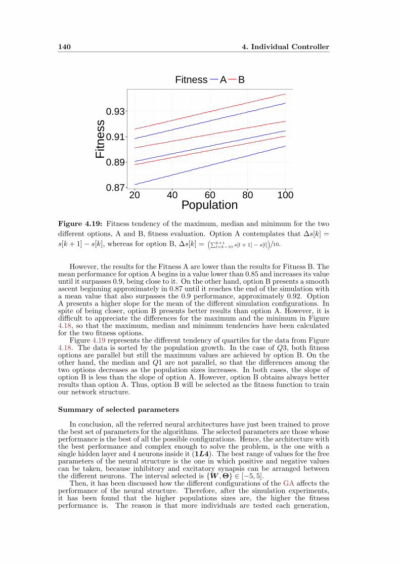
140 4. Individual Controller
0.87
0.89
0.91
0.93
20 40 60 80 100Population
Fitn
ess
Fitness A B
Figure 4.19: Fitness tendency of the maximum, median and minimum for the two
different options, A and B, fitness evaluation. Option A contemplates that ∆s[k] =
s[k + 1]− s[k], whereas for option B, ∆s[k] =(∑k+1
l=k−10 s[l + 1] − s[l])/10.
However, the results for the Fitness A are lower than the results for Fitness B. Themean performance for option A begins in a value lower than 0.85 and increases its valueuntil it surpasses 0.9, being close to it. On the other hand, option B presents a smoothascent beginning approximately in 0.87 until it reaches the end of the simulation witha mean value that also surpasses the 0.9 performance, approximately 0.92. OptionA presents a higher slope for the mean of the different simulation configurations. Inspite of being closer, option B presents better results than option A. However, it isdifficult to appreciate the differences for the maximum and the minimum in Figure4.18, so that the maximum, median and minimum tendencies have been calculatedfor the two fitness options.
Figure 4.19 represents the different tendency of quartiles for the data from Figure4.18. The data is sorted by the population growth. In the case of Q3, both fitnessoptions are parallel but still the maximum values are achieved by option B. On theother hand, the median and Q1 are not parallel, so that the differences among thetwo options decreases as the population sizes increases. In both cases, the slope ofoption B is less than the slope of option A. However, option B obtains always betterresults than option A. Thus, option B will be selected as the fitness function to trainour network structure.
Summary of selected parameters
In conclusion, all the referred neural architectures have just been trained to provethe best set of parameters for the algorithms. The selected parameters are those whoseperformance is the best of all the possible configurations. Hence, the architecture withthe best performance and complex enough to solve the problem, is the one with asingle hidden layer and 4 neurons inside it (1L4). The best range of values for the freeparameters of the neural structure is the one in which positive and negative valuescan be taken, because inhibitory and excitatory synapsis can be arranged betweenthe different neurons. The interval selected is W ,Θ ∈ [−5, 5].
Then, it has been discussed how the different configurations of the GA affects theperformance of the neural structure. Therefore, after the simulation experiments,it has been found that the higher populations sizes are, the higher the fitnessperformance is. The reason is that more individuals are tested each generation,
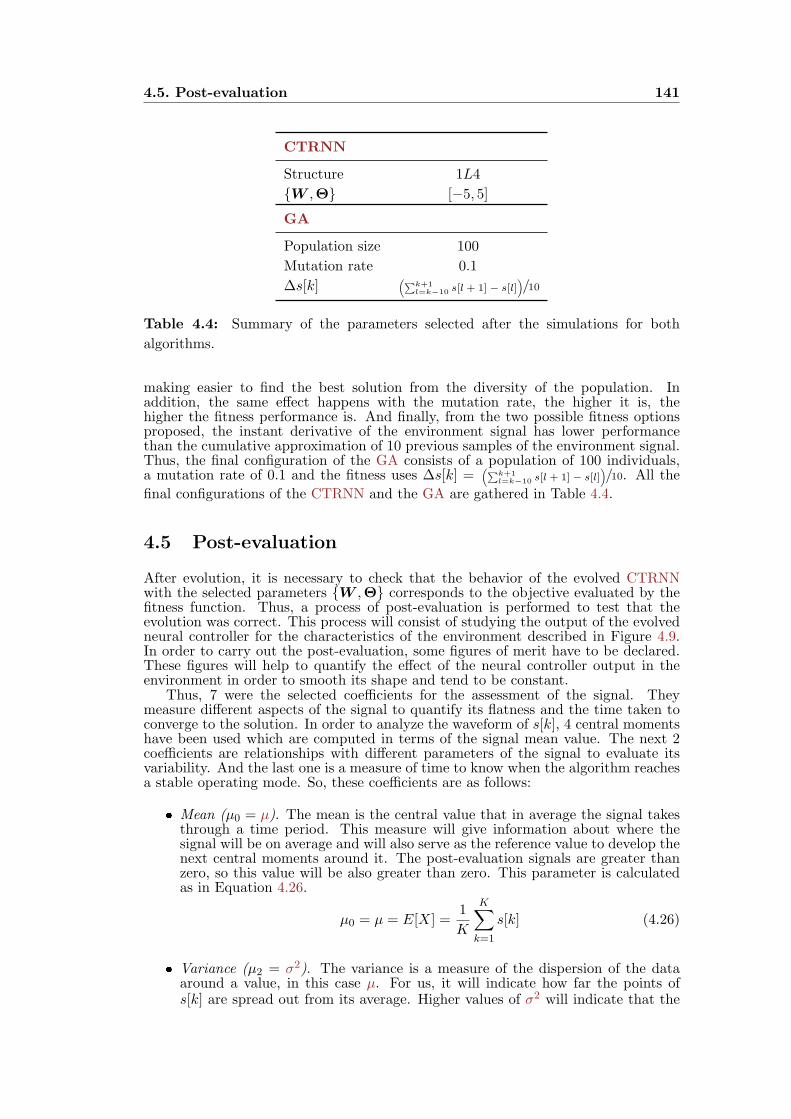
4.5. Post-evaluation 141
CTRNN
Structure 1L4
W ,Θ [−5, 5]
GA
Population size 100
Mutation rate 0.1
∆s[k](∑k+1
l=k−10 s[l + 1] − s[l])/10
Table 4.4: Summary of the parameters selected after the simulations for both
algorithms.
making easier to find the best solution from the diversity of the population. Inaddition, the same effect happens with the mutation rate, the higher it is, thehigher the fitness performance is. And finally, from the two possible fitness optionsproposed, the instant derivative of the environment signal has lower performancethan the cumulative approximation of 10 previous samples of the environment signal.Thus, the final configuration of the GA consists of a population of 100 individuals,a mutation rate of 0.1 and the fitness uses ∆s[k] =
(∑k+1l=k−10 s[l + 1] − s[l]
)/10. All the
final configurations of the CTRNN and the GA are gathered in Table 4.4.
4.5 Post-evaluation
After evolution, it is necessary to check that the behavior of the evolved CTRNNwith the selected parameters W ,Θ corresponds to the objective evaluated by thefitness function. Thus, a process of post-evaluation is performed to test that theevolution was correct. This process will consist of studying the output of the evolvedneural controller for the characteristics of the environment described in Figure 4.9.In order to carry out the post-evaluation, some figures of merit have to be declared.These figures will help to quantify the effect of the neural controller output in theenvironment in order to smooth its shape and tend to be constant.
Thus, 7 were the selected coefficients for the assessment of the signal. Theymeasure different aspects of the signal to quantify its flatness and the time taken toconverge to the solution. In order to analyze the waveform of s[k], 4 central momentshave been used which are computed in terms of the signal mean value. The next 2coefficients are relationships with different parameters of the signal to evaluate itsvariability. And the last one is a measure of time to know when the algorithm reachesa stable operating mode. So, these coefficients are as follows:
Mean (µ0 = µ). The mean is the central value that in average the signal takesthrough a time period. This measure will give information about where thesignal will be on average and will also serve as the reference value to develop thenext central moments around it. The post-evaluation signals are greater thanzero, so this value will be also greater than zero. This parameter is calculatedas in Equation 4.26.
µ0 = µ = E[X] =1
K
K∑k=1
s[k] (4.26)
Variance (µ2 = σ2). The variance is a measure of the dispersion of the dataaround a value, in this case µ. For us, it will indicate how far the points ofs[k] are spread out from its average. Higher values of σ2 will indicate that the
142 4. Individual Controller
variability of the signal is too high, while a zero value indicates that all valueswill be the same, so that s[k] will be constant. σ2 is the second central momentand its mathematical expression is as follows:
µ2 = σ2 = E[(X −E [X])2
]=
1
K
K∑k=1
(s[k]− µ)2 (4.27)
Skewness (µ3). This parameter measures the asymmetry of the data, if it isabove or below µ. Thus, it indicates how the signal is distributed around itsaverage in a time period. It can be interpreted for positive values as the signalis above µ most of the time. Whereas if it is below µ, it indicates that most ofthe time the signal is below the data. In case of 0, the data is around the mean.This is the third central moment and it is calculated as:
µ3 = E[(X − E [X])3
]=
1K
∑Kk=1(s[k]− µ)3
σ3(4.28)
Kurtosis (µ4). This is another measure of the form of the signal as µ4. In thiscase, the kurtosis is studying the dispersion of a signal related to the averagethrough the points closest to it compared with those points of the distant ends.Therefore, a high value of µ4 means that there are lots of points around themean but at the same time lots of them are also in the ends of the signal.On the contrary, a low value means that all the points are concentrated in theaverage of the signal. The mathematical expression is:
µ4 = E[(X − E [X])4
]=
1K
∑Kk=1(s[k]− µ)4
σ4(4.29)
Coefficient of variation (cv). This parameter establishes a relationship betweenthe average of the signal and its variance. When the data is around the mean,this coefficient is next to 0 and otherwise the data will present mean deviations.This coefficient is described mathematically in Equation 4.30.
cv =σ
µ(4.30)
Crest factor (Cf ). The last parameter related with the form of the signal is thecrest factor. This factor measures the waveform through the ratio of maximumvalues of the signals compared to its effective value. Thus, it indicates how highthe peaks are present in the form of the signal. A Cf of 1 indicates that thesignal does not have any present peak and it is constant, whereas higher valuesindicates how accused those peaks are. This factor compares the maximum ofa signal with respect to Root Mean Square (rms) of the signal for a time period(see Equation 4.31).
Cf =|s|peaksrms
∣∣∣∣K
(4.31)
Time of convergence (tc). The last parameter used is the convergence timeof the neural controller to flatten the environment signal. It is a measure ofthe stability of the algorithm indicating when the signal becomes stable andabandons the transitory state. Hence, it is considered that the environment hasreached a stable state when the σ2 is less than an established minimum duringa period of time. This is expressed in Equation 4.32.
tc = |σ2| < σ2min
∣∣K (4.32)
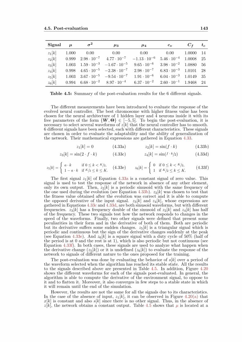
4.5. Post-evaluation 143
Signal µ σ2 µ3 µ4 cv Cf tc
z1[k] 1.000 0.00 0.00 0.00 0.00 1.0000 14
z2[k] 0.999 2.98 · 10−7 4.77 · 10−7 −1.13 · 10−6 5.46 · 10−4 1.0008 25
z3[k] 1.003 1.59 · 10−3 −1.67 · 10−5 9.65 · 10−6 3.98 · 10−2 1.0880 56
z4[k] 0.998 4.65 · 10−5 −2.38 · 10−7 2.98 · 10−7 6.83 · 10−3 1.0101 28
z5[k] 1.003 3.67 · 10−5 −9.54 · 10−7 1.91 · 10−6 6.04 · 10−3 1.0149 35
z6[k] 0.994 6.68 · 10−2 8.97 · 10−4 6.37 · 10−2 2.60 · 10−1 1.9468 24
Table 4.5: Summary of the post-evaluation results for the 6 different signals.
The different measurements have been introduced to evaluate the response of theevolved neural controller. The best chromosome with higher fitness value has beenchosen for the neural architecture of 1 hidden layer and 4 neurons inside it with itsfree parameters of the form W ,Θ ∈ [−5, 5]. To begin the post-evaluation, it isnecessary to select several waveforms of z[k] that the neural controller has to smooth.6 different signals have been selected, each with different characteristics. These signalsare chosen in order to evaluate the adaptability and the ability of generalization ofthe network. Their mathematical expressions are gathered in Equation 4.33.
z1[k] = 0 (4.33a) z2[k] = sin(f · k) (4.33b)
z3[k] = sin(2 · f · k) (4.33c) z4[k] = sin(f · k/2) (4.33d)
z5[k] =
a · k if 0 ≤ k < K/2,
1− a · k if K/2 ≤ k ≤ K.(4.33e) z6[k] =
0 if 0 ≤ k < K/2,
1 if K/2 ≤ k ≤ K.(4.33f)
The first signal z1[k] of Equation 4.33a is a constant signal of zero value. Thissignal is used to test the response of the network in absence of any other element,only its own output. Then, z2[k] is a periodic sinusoid with the same frequency ofthe one used during the evolution (see Equation 4.33b). z2[k] was chosen to test thatthe fitness value obtained after the evolution was correct and it is able to computethe opposed derivative of the input signal. z3[k] and z4[k], whose expressions aregathered in Equations 4.33c and 4.33d, are both sinusoid waveforms, but with differentfrequencies. z3[k] has a frequency double of the sinusoid of z2[k] and z4[k] has halfof the frequency. These two signals test how the network responds to changes in thespeed of the waveforms. Finally, two other signals were defined that present somepeculiarities in their form and in the derivative of both of them. Both are periodicbut its derivative suffers some sudden changes. z5[k] is a triangular signal which isperiodic and continuous but the sign of the derivative changes suddenly at the peak(see Equation 4.33e). And z6[k] is a square signal with a duty cycle of 50% (half ofthe period is at 0 and the rest is at 1), which is also periodic but not continuous (seeEquation 4.33f). In both cases, these signals are used to analyze what happen whenthe derivative change (z5[k]) or it is undefined (z6[k]) to evaluate the response of thenetwork to signals of different nature to the ones proposed for the training.
The post-evaluation was done by evaluating the behavior of s[k] over a period ofthe waveform selected when the algorithm has reached its stable state. All the resultsto the signals described above are presented in Table 4.5. In addition, Figure 4.20shows the different waveforms for each of the signals post-evaluated. In general, thealgorithm is able to compute the derivative of the environment signal, to oppose toit and to flatten it. Moreover, it also converges in few steps to a stable state in whichit will remain until the end of the simulation.
However, the results are not the same for all the signals due to its characteristics.In the case of the absence of input, z1[k], it can be observed in Figure 4.20(a) thatx[k] is constant and also s[k] since there is no other signal. Thus, in the absence ofz[k], the network obtains a constant output. Table 4.5 shows that µ is located at a
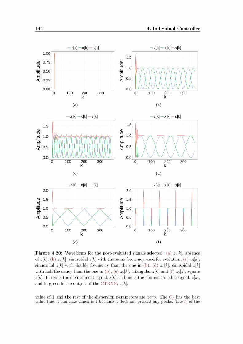
144 4. Individual Controller
0.00
0.25
0.50
0.75
1.00
0 100 200 300k
Am
plitu
de
z[k] x[k] s[k]
(a)
0.0
0.5
1.0
1.5
0 100 200 300k
Am
plitu
de
z[k] x[k] s[k]
(b)
0.0
0.5
1.0
1.5
0 100 200 300k
Am
plitu
de
z[k] x[k] s[k]
(c)
0.0
0.5
1.0
1.5
0 100 200 300k
Am
plitu
dez[k] x[k] s[k]
(d)
0.0
0.5
1.0
1.5
2.0
0 100 200 300k
Am
plitu
de
z[k] x[k] s[k]
(e)
0.0
0.5
1.0
1.5
2.0
0 100 200 300k
Am
plitu
de
z[k] x[k] s[k]
(f)
Figure 4.20: Waveforms for the post-evaluated signals selected: (a) z1[k], absence
of z[k], (b) z2[k], sinusoidal z[k] with the same frecuency used for evolution, (c) z3[k],
sinusoidal z[k] with double frequency than the one in (b), (d) z4[k], sinusoidal z[k]
with half frecuency than the one in (b), (e) z5[k], triangular z[k] and (f) z6[k], square
z[k]. In red is the environment signal, s[k], in blue is the non-controllable signal, z[k],
and in green is the output of the CTRNN, x[k].
value of 1 and the rest of the dispersion parameters are zero. The Cf has the bestvalue that it can take which is 1 because it does not present any peaks. The tc of the

4.5. Post-evaluation 145
Signal zCf sCf∆Cf/sCf
[%]
z1[k] – 1 0
z2[k] 1.63065 1.00083 62.9302
z3[k] 1.63137 1.08802 49.9397
z4[k] 1.63166 1.01013 61.5298
z5[k] 1.32944 1.01495 30.9859
z6[k] 2.27303 1.94682 16.7563
Table 4.6: Comparison of Cf with and without the evolved neural controller.
network is quickly, in 14 time steps it reaches the stable state in which it will remainuntil the end.
The next signal, z2[k] is the same signal used for the training, so it is expected ahigh performance. Table 4.5 shows that s[k] is centered in 1 again and there is notany dispersion around µ. Its σ2 is negligible, the skew of the signal is near zero andthey are very concentrated in the mean since the kurtosis is also negligible. The cvalso indicates that the dispersion of the data is small and Cf confirms the absence ofpeaks for s[k] since is near to the optimum. tc is again very low in 25 time steps thealgorithm has already converged. The waveforms of Figure 4.20(b) show that x[k] isin antiphase to z2[k] to produce a flattened s[k].
z3[k] and z4[k] are again two sinusoids to prove the behavior of the network whenthe frequency of the sinusoid varies. In the case of z3[k], it can be observed in Figure4.20(c) that the controller does not behave as great as in Figure 4.20(b), because itpresents a ripple in s[k]. In Table 4.5, the moments σ2, µ3 and µ4 are higher than onesfor z2[k] so the data dispersion is bigger. And also the form of the waveform presentssome peaks that are also present in the value of Cf . In addition, tc is approximatelydouble the one of z2[k]. On the contrary, when the frequency is lower, the results arevery similar to the one obtained for z2[k]. Low values for the dispersion coefficients,σ2, µ3, µ4 and cv. And also a very close value of Cf to 1, so that it has not anypronounced peak. tc is also as low as z2[k]. Thus, the neural controller behavessimilar for frequencies less than the one selected for the evolution. For frequencieshigher than the one selected in the evolution they reduce the variability of the signalbut they present some peaks in the resultant waveform.
z5[k] has little dispersion around the mean as the value of the σ2 and cv are low(see Table 4.5). In addition, the data is concentrated in the mean and with no skewabove or below due to moments µ3 and µ4 are also low. The waveform is also reallyflatten as it can be seen in Figure 4.20(e) and checked with a Cf close to 1. And theconvergence time is low, only 35 time steps. On the other hand, the performance ofz6[k] is the worst compared to the rest of signals. There is more dispersion aroundthe mean because the σ2, µ4 and cv are higher compared to the rest. The data is notskewed because it presents a relative low value. About the form in Figure 4.20(f), thepresence of peaks can be observed at the point in which the signal changes of state.Therefore, Cf has a high value far from 1 because of the presence of those peaks.However, the response of the network is very fast and in only 24 steps the networkhas converged.
Table 4.6 shows a comparison summary of the algorithm application. In the caseof z1[k], there is no improvement due to the absence of signal at the input of thenetwork. There is a reduction of Cf in all cases. In the best of the cases (for signalsz2[k] and z4[k]), a reduction of the 60% was achieved. Whereas in the worst case (forsignal z6[k]), a reduction of 15% was achieved. Thus, the application of the algorithmalways reduces the peaks, increasing the flattening of the s[k].
A last trial was carried out in order to test how the neural controller performswith a signal similar to the grid aggregated consumption. Thus, an artificial grid
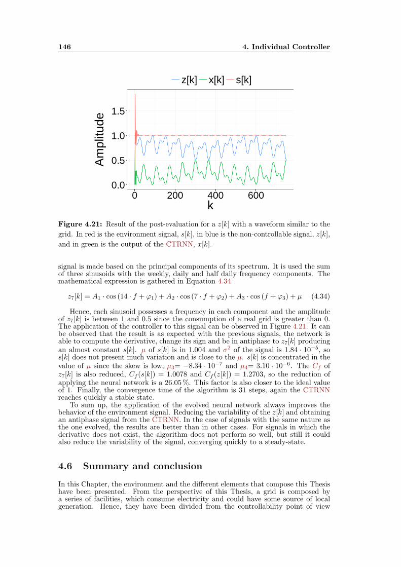
146 4. Individual Controller
0.0
0.5
1.0
1.5
0 200 400 600k
Am
plitu
de
z[k] x[k] s[k]
Figure 4.21: Result of the post-evaluation for a z[k] with a waveform similar to the
grid. In red is the environment signal, s[k], in blue is the non-controllable signal, z[k],
and in green is the output of the CTRNN, x[k].
signal is made based on the principal components of its spectrum. It is used the sumof three sinusoids with the weekly, daily and half daily frequency components. Themathematical expression is gathered in Equation 4.34.
z7[k] = A1 · cos (14 · f + φ1) +A2 · cos (7 · f + φ2) +A3 · cos (f + φ3) + µ (4.34)
Hence, each sinusoid possesses a frequency in each component and the amplitudeof z7[k] is between 1 and 0.5 since the consumption of a real grid is greater than 0.The application of the controller to this signal can be observed in Figure 4.21. It canbe observed that the result is as expected with the previous signals, the network isable to compute the derivative, change its sign and be in antiphase to z7[k] producingan almost constant s[k]. µ of s[k] is in 1.004 and σ2 of the signal is 1.84 · 10−5, sos[k] does not present much variation and is close to the µ. s[k] is concentrated in thevalue of µ since the skew is low, µ3= −8.34 · 10−7 and µ4= 3.10 · 10−6. The Cf ofz7[k] is also reduced, Cf (s[k]) = 1.0078 and Cf (z[k]) = 1.2703, so the reduction ofapplying the neural network is a 26.05%. This factor is also closer to the ideal valueof 1. Finally, the convergence time of the algorithm is 31 steps, again the CTRNNreaches quickly a stable state.
To sum up, the application of the evolved neural network always improves thebehavior of the environment signal. Reducing the variability of the z[k] and obtainingan antiphase signal from the CTRNN. In the case of signals with the same nature asthe one evolved, the results are better than in other cases. For signals in which thederivative does not exist, the algorithm does not perform so well, but still it couldalso reduce the variability of the signal, converging quickly to a steady-state.
4.6 Summary and conclusion
In this Chapter, the environment and the different elements that compose this Thesishave been presented. From the perspective of this Thesis, a grid is composed bya series of facilities, which consume electricity and could have some source of localgeneration. Hence, they have been divided from the controllability point of view
4.6. Summary and conclusion 147
of its consumption in controllable and non-controllable facilities. The objective ofthis Thesis, consists of reducing the variability of the aggregated consumption of thedifferent users. However, this problem is too complex to solve in one step so it hasbeen simplified by dividing the environment in only two blocks, one controllable andone non-controllable.
Then, different possibilities have been considered in order to flatten the aggrega-tion of the different users. In this way, it is thought that cancelling the derivativeof the non-controllable signal will be enough to obtain a constant aggregated signal.So, the derivative algorithm followed was explained in order to create a destructiveinterference that will be in antiphase to the one corresponding to the non-controllableusers. This approach was possible due to the properties of the CTRNN inside thecontrollable user. A signal processing approach was followed to understand theproblem and simplify it. Rather than using the grid aggregated consumption, astage was used in which the non-controllable demand, z(t), was sinusoidal. Thus, theCTRNN has to produce the antiphase output in order to obtain an s(t) flatten.
In spite of having stated the problem, the neural architecture was not clear and itwas necessary to develop a series of experiments to have the best performance network.388800 simulations were conducted to obtain the best neural architecture consistingof 1 input layer with 2 neurons, 1 hidden layer with 4 neurons and 1 output layer withonly 1 neuron corresponding to the output of the neural controller taking values forthe free parameters inside the interval [−5, 5]. To find this architecture, 12 differentstructures have been evolved with 6 ranges of values for the free parameters of thenetwork. The GA used for the evolution has different sizes of populations (20–100) anddifferent mutation rates (0.01–0.1). To evaluate the performance, a fitness functionwas defined using the concept of cancelling the derivative of the environment signal toobtain a constant one. Each experiment was initialized 30 times with different seedsto randomize the beginning initial conditions of the simulation.
Once the architecture and the configuration of the GA were obtained, the behaviorof the best chromosome was checked with different signals. A series of post-evaluationexperiments have been done in which the first 4th central moments and the cv wereanalyzed to know more about the dispersion of the signal around its mean, checking ifit is enough flattened. Then, the Cf was evaluated to know the form of the resultantenvironment signal and if it presents some peaks on it. Last parameter is the timeof convergence of the algorithm or the number of steps that the algorithm takesto reach a stable state. These coefficients were tested with seven different signalswhich possesses different characteristics: i) absence of z[k], to test the stability of thearchitecture, ii) sinusoid of the same frequency as the one trained, iii) sinusoid of thedouble of frequency, iv) sinusoid half of the frequency, v) triangular, to understandthe behavior when there are points with no derivate, vi) square, to understand whathappens when there are discontinuities, and vii) sum of sinusoids, imitating the gridaggregated consumption in order to see the potential of the controller developed. In allthe cases good results were achieved, in the case in which the derivate is not defined,v) and vi), it was able to reduce its variability but not as well as with continuous andclass C1 signals. With abrupt changes (triangular), the controller is able to produce aflattened s[k], however with discontinuities (square), is almost impossible and peaksare produced at the discontinuity point. In the best of the cases, the peaks werereduced around the 60% and in the worst case a 16%. In the case of the artificialsignal of the grid, the Cf was near to 1 and it was reduced a 26.05%. Thus, it canbe concluded that these results are good enough to follow with the next step of theproblem, the collective behavior of the controllable users described in Chapter 5.

148 4. Individual Controller

5Collective Controller“The ones who are crazy enough to think that they can change
the world, are the ones who do” — Steve Jobs
Once the neural controller has been evolved, a part of the problem hasbeen solved in a reduced environment. However, it is necessary toadvance on the complete problem presented in Section 4.1. To thatend, this Chapter goes a step further and adds more complexity to the
environment by putting more individuals of the two types in which the grid is divided.The addition of more controllable and non-controllable users threatens the neuralcontroller developed in Chapter 4. The reason is that the controller was designed inorder to smooth the demand when the controllable power is half the power of thesystem (the other half is coming from the non-controllable user). In this way, theneural controller was able to achieve good results and the difference between valleysand peaks was reduced.
As explained in Chapter 4, the central block of the distributed system has beendesigned based on the tendency of the derivative. This block is a dynamic systemconsisting of a Continuous Time RNN (CTRNN) that behaves in antiphase to anunknown signal. Its output, added to the non-controllable signal, cancels the variancein the resultant signal and generates a constant one. Thus, a first approach consistsof using this neural controller for all the controllable users, in order to generate theantiphase signal. Figure 5.1 shows the response of an environment in which aroundthe 65% of the signal comes from controllable sources and the remaining 35% isfrom non-controllable sources. It can be observed that each individual xi[k] putsthe same exact quantity of signal and their aggregation produced more peaks in theenvironment signal without leaving their transitory state. However, this approachmay incur in a serious problem of instability depending on the size of the environmentsince all the neural controllers behave the same. In addition, there are some otherissues related with the nature of the controller, such as the output range (between[0, 1] due to the sigmoid function) or the level of the input signal to the network sinceits output is bounded.
On the other hand, a real grid is a heterogeneous environment in which one ofthe methods used to smooth the demand curve consists of the aggregation of moreloads to the system and augmenting the diversity inside it. As discussed in Section2.1.5, the consumption of residential and service sectors present a variability thatrepeats periodically. The habits of users are very similar and repeat along the timebut they are not the same. Therefore, the use of the same neural controller for allthe controllable users provide the same response for each of them. At the time toaggregate their consumption, new peaks are found when the valley of the demandcurve occurs because the controller will try to displace the consumption at thosepoints. Thus, it is necessary to coordinate the different controllable individuals tocontinue having a flattened curve and not to get a worse situation than the beginning.
But how can a population of neural controllers be coordinated when there is nocommunication among them? The answer to this question can be easily tackled whenthe different parts and blocks of the system are interconnected creating a completeneural system. The reason is that synaptic connections are used to regulate the pass ofinformation along different parts of the neural system. Thus, with enough connectionsamong the controllers, their output could be regulated with some inhibitory or
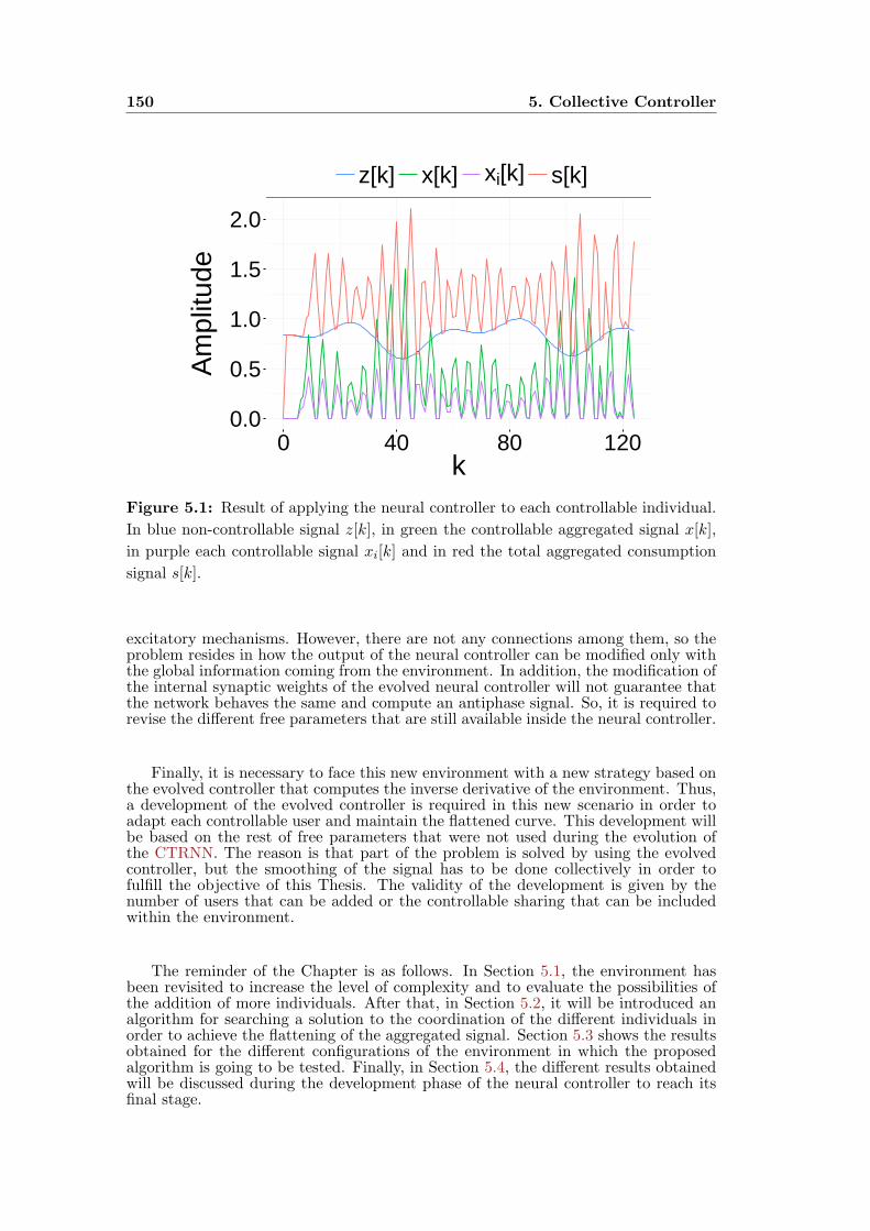
150 5. Collective Controller
0.0
0.5
1.0
1.5
2.0
0 40 80 120k
Am
plitu
dez[k] x[k] xi[k] s[k]
Figure 5.1: Result of applying the neural controller to each controllable individual.
In blue non-controllable signal z[k], in green the controllable aggregated signal x[k],
in purple each controllable signal xi[k] and in red the total aggregated consumption
signal s[k].
excitatory mechanisms. However, there are not any connections among them, so theproblem resides in how the output of the neural controller can be modified only withthe global information coming from the environment. In addition, the modification ofthe internal synaptic weights of the evolved neural controller will not guarantee thatthe network behaves the same and compute an antiphase signal. So, it is required torevise the different free parameters that are still available inside the neural controller.
Finally, it is necessary to face this new environment with a new strategy based onthe evolved controller that computes the inverse derivative of the environment. Thus,a development of the evolved controller is required in this new scenario in order toadapt each controllable user and maintain the flattened curve. This development willbe based on the rest of free parameters that were not used during the evolution ofthe CTRNN. The reason is that part of the problem is solved by using the evolvedcontroller, but the smoothing of the signal has to be done collectively in order tofulfill the objective of this Thesis. The validity of the development is given by thenumber of users that can be added or the controllable sharing that can be includedwithin the environment.
The reminder of the Chapter is as follows. In Section 5.1, the environment hasbeen revisited to increase the level of complexity and to evaluate the possibilities ofthe addition of more individuals. After that, in Section 5.2, it will be introduced analgorithm for searching a solution to the coordination of the different individuals inorder to achieve the flattening of the aggregated signal. Section 5.3 shows the resultsobtained for the different configurations of the environment in which the proposedalgorithm is going to be tested. Finally, in Section 5.4, the different results obtainedwill be discussed during the development phase of the neural controller to reach itsfinal stage.
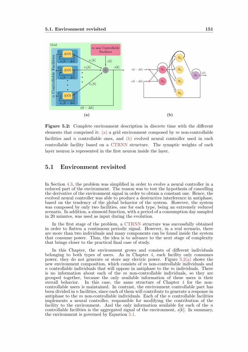
5.1. Environment revisited 151
Grid
C1
C2
Cn
ANN
m non ControllableFacilities
ANN +
ANN
z[k]x1[k]
x2[k]
xn[k]
s[k]
x1[k −∆k]
x2[k −∆k]
xn[k −∆k]
s[k −∆k]
nCon
trollable
Facilities
(a)
N3
N1 N4
N2 N5
N6
N7
x[k]
x[k −∆k]
s[k −∆k]
(b)
Figure 5.2: Complete environment description in discrete time with the different
elements that comprised it: (a) a grid environment composed by m non-controllable
facilities and n controllable ones, and (b) evolved neural controller used in each
controllable facility based on a CTRNN structure. The synaptic weights of each
layer neuron is represented in the first neuron inside the layer.
5.1 Environment revisited
In Section 4.3, the problem was simplified in order to evolve a neural controller in areduced part of the environment. The reason was to test the hypothesis of cancellingthe derivative of the environment signal in order to obtain a constant one. Hence, theevolved neural controller was able to produce a destructive interference in antiphase,based on the tendency of the global behavior of the system. However, the systemwas composed by only two facilities, one for each type, being an extremely reducedscenario. In addition, a sinusoid function, with a period of a consumption day sampledin 20 minutes, was used as input during the evolution.
In the first stage of the problem, a CTRNN structure was successfully obtainedin order to flatten a continuous periodic signal. However, in a real scenario, thereare more than two individuals and many components can be found inside the systemthat consume power. Thus, the idea is to advance to the next stage of complexitythat brings closer to the practical final case of study.
In this Chapter, the environment grows and consists of different individualsbelonging to both types of users. As in Chapter 4, each facility only consumespower, they do not generate or store any electric power. Figure 5.2(a) shows thenew environment composition, which consists of m non-controllable individuals andn controllable individuals that will oppose in antiphase to the m individuals. Thereis no information about each of the m non-controllable individuals, so they aregrouped together, because the only available information of these users is theiroverall behavior. In this case, the same structure of Chapter 4 for the non-controllable users is maintained. In contrast, the environment controllable part hasbeen divided in n facilities, since each of them will contribute to generate a response inantiphase to the m non-controllable individuals. Each of the n controllable facilitiesimplements a neural controller, responsible for modifying the contribution of thefacility to the environment. And the only information available for each of the ncontrollable facilities is the aggregated signal of the environment, s[k]. In summary,the environment is governed by Equation 5.1.
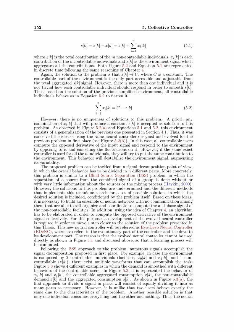
152 5. Collective Controller
s[k] = z[k] + x[k] = z[k] +n∑
i=1
xi[k] (5.1)
where z[k] is the total contribution of the m non-controllable individuals, xi[k] is eachcontribution of the n controllable individuals and s[k] is the environment signal whichaggregates all the contributions. Both Figure 5.2 and Equation 5.1 are representedin discrete time following the same reasoning of Chapter 4.
Again, the solution to the problem is that s[k]→ C, where C is a constant. Thecontrollable part of the environment is the only part accessible and adjustable fromthe total aggregated s[k] signal. However, there is more than one individual and it isnot trivial how each controllable individual should respond in order to smooth s[k].Thus, based on the solution of the previous simplified environment, all controllableindividuals behave as in Equation 5.2 to flatten it.
n∑i=1
xi[k] = C − z[k] (5.2)
However, there is no uniqueness of solutions to this problem. A priori, anycombination of xi[k] that will produce a constant s[k] is accepted as solution to thisproblem. As observed in Figure 5.2(a) and Equations 5.1 and 5.2, this environmentconsists of a generalization of the previous one presented in Section 4.1. Thus, it wasconceived the idea of using the same neural controller designed and evolved for theprevious problem in first place (see Figure 5.2(b)). In this case, all controllable userscompute the opposed derivative of the input signal and respond to the environmentby opposing to it and cancelling the fluctuations on it. However, if the same exactcontroller is used for all the n individuals, they will try to put the same contribution tothe environment. This behavior will destabilize the environment signal, augmentingits variability.
The proposed problem can be tackled from a signal decomposition point of view,in which the overall behavior has to be divided in n different parts. More concretely,this problem is similar to a Blind Source Separation (BSS) problem, in which theseparation of a source from the combined signal of a group is done without orwith very little information about the sources or the mixing process (Haykin, 2000).However, the solutions to this problem are undetermined and the different methodsthat implements this technique search for a set of possible solutions in which thedesired solution is included, conditioned by the problem itself. Based on these ideas,it is necessary to build an ensemble of neural networks with no communication amongthem that are able to self-organize and coordinate to compute the antiphase signal ofthe non-controllable facilities. In addition, using the idea of Chapter 4, an algorithmhas to be elaborated in order to compute the opposed derivative of the environmentsignal collectively. For this purpose, a development of the evolved neural controlleris required in order to move a step closer to the solution of the problem presented inthis Thesis. This new neural controller will be referred as Evo-Devo Neural Controller(EDeNC), where evo refers to the evolutionary part of the controller and the devo toits development part. The reason is that the evolved neural controller cannot be useddirectly as shown in Figure 5.1 and discussed above, so that a learning process willbe computed.
Following the BSS approach to the problem, numerous signals accomplish thesignal decomposition proposed in first place. For example, in case the environmentis composed by 2 controllable individuals (facilities, x0[k] and x1[k]) and 1 non-controllable (z[k]), there exist multiple waveforms that can accomplish the task.Figure 5.3 shows 4 different examples in which the demand is smoothed with differentbehaviors of the controllable users. In Figure 5.3, it is represented the behavior ofx0[k] and x1[k], the controllable aggregated consumption x[k], the non-controllabledemand z[k] and the aggregated consumption s[k]. As shown in Figure 5.3(a), thefirst approach to divide a signal in parts will consist of equally dividing it into asmany parts as necessary. However, it is unlike that two users behave exactly thesame due to the characteristics of the problem. Another possible solution is thatonly one individual consumes everything and the other one nothing. Thus, the neural
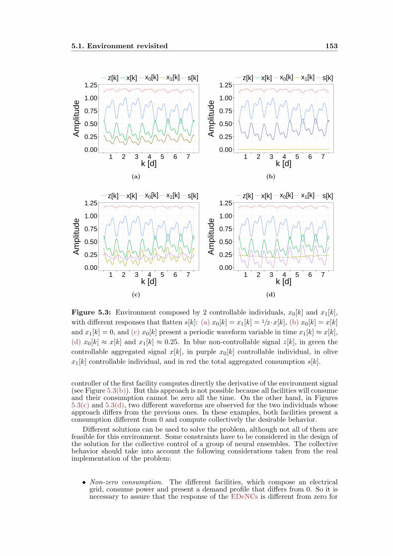
5.1. Environment revisited 153
0.00
0.25
0.50
0.75
1.00
1.25
1 2 3 4 5 6 7k [d]
Am
plitu
dez[k] x[k] x0[k] x1[k] s[k]
(a)
0.00
0.25
0.50
0.75
1.00
1.25
1 2 3 4 5 6 7k [d]
Am
plitu
de
z[k] x[k] x0[k] x1[k] s[k]
(b)
0.00
0.25
0.50
0.75
1.00
1.25
1 2 3 4 5 6 7k [d]
Am
plitu
de
z[k] x[k] x0[k] x1[k] s[k]
(c)
0.00
0.25
0.50
0.75
1.00
1.25
1 2 3 4 5 6 7k [d]
Am
plitu
de
z[k] x[k] x0[k] x1[k] s[k]
(d)
Figure 5.3: Environment composed by 2 controllable individuals, x0[k] and x1[k],
with different responses that flatten s[k]: (a) x0[k] = x1[k] = 1/2 ·x[k], (b) x0[k] = x[k]
and x1[k] = 0, and (c) x0[k] present a periodic waveform variable in time x1[k] ≈ x[k],
(d) x0[k] ≈ x[k] and x1[k] ≈ 0.25. In blue non-controllable signal z[k], in green the
controllable aggregated signal x[k], in purple x0[k] controllable individual, in olive
x1[k] controllable individual, and in red the total aggregated consumption s[k].
controller of the first facility computes directly the derivative of the environment signal(see Figure 5.3(b)). But this approach is not possible because all facilities will consumeand their consumption cannot be zero all the time. On the other hand, in Figures5.3(c) and 5.3(d), two different waveforms are observed for the two individuals whoseapproach differs from the previous ones. In these examples, both facilities present aconsumption different from 0 and compute collectively the desirable behavior.
Different solutions can be used to solve the problem, although not all of them arefeasible for this environment. Some constraints have to be considered in the design ofthe solution for the collective control of a group of neural ensembles. The collectivebehavior should take into account the following considerations taken from the realimplementation of the problem:
Non-zero consumption. The different facilities, which compose an electricalgrid, consume power and present a demand profile that differs from 0. So it isnecessary to assure that the response of the EDeNCs is different from zero for

154 5. Collective Controller
at least a period of time. Mathematically, this means that
∀xi with i ∈ 1, 2, . . . , n; ∃k ∈ 1, 2, . . . ,K | xi[k] = 0
Furthermore, this behaviour is repeated periodically by the facilities based onthe consumer habits. Thus, there are various time periods (several ks) inwhich the consumption is non-zero. Then, solutions, such as the one of Figure5.3(b), are not taken into account because they are not feasible for this kind ofenvironment.
Heterogeneous demand profiles. The demand profiles of the different facilitiesof an electrical grid are not the same. They are grouped together dependingon the typical loads that generate those consumption profiles. Although theyhave similar loads, the demand profile is not exactly the same because usersconsume based on their necessities at different time periods. So, the EDeNCshould produce different outputs for each controllable facility. They can besimilar but not the same. Thus, solutions, such as the one of Figure 5.3(a), arepossible but not reasonable for a real implementation.
Scalability. Another aspect of the environment is the number of individuals whoare part of it. It is necessary that the algorithm can operate independently ofthe number of users and adapt the output of the controllable ones to the non-controllable in order to smooth the aggregated demand curve. The proposeddistributed control solution has to be able to adapt to the different possiblescenarios in which the contribution of the users can vary. The environment canbe composed of different combinations of m and n users, in which m can beless, equal or greater than n. Thus, the n controllable users should always reactand do their best effort in order to flatten the aggregated demand curve. Inaddition, the algorithm should be able to react to any size of the controllableusers or to the incorporation of new users into the environment.
Real time operation. The last aspect to consider is its operation. It is requiredthat the EDeNCs can adapt to the changes in the environment. So, theEDeNC learning algorithm has to adapt to those changes since the grid evolvesconstantly. This adaptation process should be fast enough to respond to changesin demand and able to react to any modification occurring in the environment.Then, the algorithm should operate in real time to confront these problems andthe ones derived from the environment operation.
The algorithm, proposed in this Chapter, should be built taking into accountthese four aspects for the development of the evolved neural controllers. However,once the neural controller is evolved, the different parameters of the network are fixedand it behaves as the antiphase signal for the non-controllable users. Thus, a firstapproximation could be based on retuning W ,Θ in order to adapt the output ofeach controller. There exist various problems to this approximation. The first one isthat the Genetic Algorithm (GA) proposed in Chapter 4 cannot be used, since theoperation has to be done in real time in order to vary those parameters. Secondly,each controller has to estimate a variation of its previous parameters to achieve thecollective flattening of the signal. Hence, it implies that the algorithm has to be fastenough in order not to interfere with the controller output. Finally, the last problemis related with the size of the environment. Depending on the algorithm construction,adding new users could destabilize the operation due to new elements or the reactionsof the algorithm could be slow.
This strategy of retuning the connections of the network is not the best strategyto tackle the problem. However, it would be more interesting to leave the networkin its evolved form and change the controller output in order to avoid overlappingwith the other users’ output. For example, the different controller outputs can bedisplaced in time. Thus, they do not overlap and the controllers parameters do nothave to be retuned. τi is the neural parameter related with time and represents themembrane time constant, related with the action potential of the neuron. The value
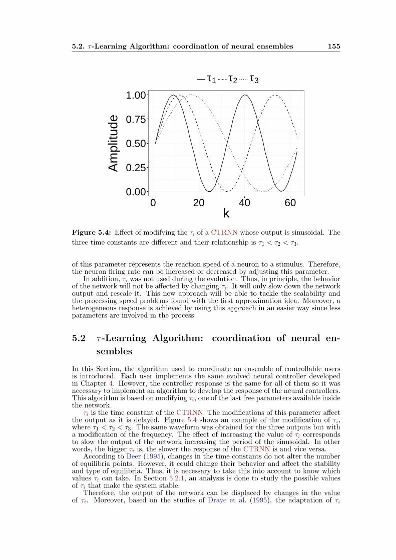
5.2. τ-Learning Algorithm: coordination of neural ensembles 155
0.00
0.25
0.50
0.75
1.00
0 20 40 60k
Am
plitu
de
τ1 τ2 τ3
Figure 5.4: Effect of modifying the τi of a CTRNN whose output is sinusoidal. The
three time constants are different and their relationship is τ1 < τ2 < τ3.
of this parameter represents the reaction speed of a neuron to a stimulus. Therefore,the neuron firing rate can be increased or decreased by adjusting this parameter.
In addition, τi was not used during the evolution. Thus, in principle, the behaviorof the network will not be affected by changing τi. It will only slow down the networkoutput and rescale it. This new approach will be able to tackle the scalability andthe processing speed problems found with the first approximation idea. Moreover, aheterogeneous response is achieved by using this approach in an easier way since lessparameters are involved in the process.
5.2 τ-Learning Algorithm: coordination of neural en-
sembles
In this Section, the algorithm used to coordinate an ensemble of controllable usersis introduced. Each user implements the same evolved neural controller developedin Chapter 4. However, the controller response is the same for all of them so it wasnecessary to implement an algorithm to develop the response of the neural controllers.This algorithm is based on modifying τi, one of the last free parameters available insidethe network.
τi is the time constant of the CTRNN. The modifications of this parameter affectthe output as it is delayed. Figure 5.4 shows an example of the modification of τi,where τ1 < τ2 < τ3. The same waveform was obtained for the three outputs but witha modification of the frequency. The effect of increasing the value of τi correspondsto slow the output of the network increasing the period of the sinusoidal. In otherwords, the bigger τi is, the slower the response of the CTRNN is and vice versa.
According to Beer (1995), changes in the time constants do not alter the numberof equilibria points. However, it could change their behavior and affect the stabilityand type of equilibria. Thus, it is necessary to take this into account to know whichvalues τi can take. In Section 5.2.1, an analysis is done to study the possible valuesof τi that make the system stable.
Therefore, the output of the network can be displaced by changes in the valueof τi. Moreover, based on the studies of Draye et al. (1995), the adaptation of τi
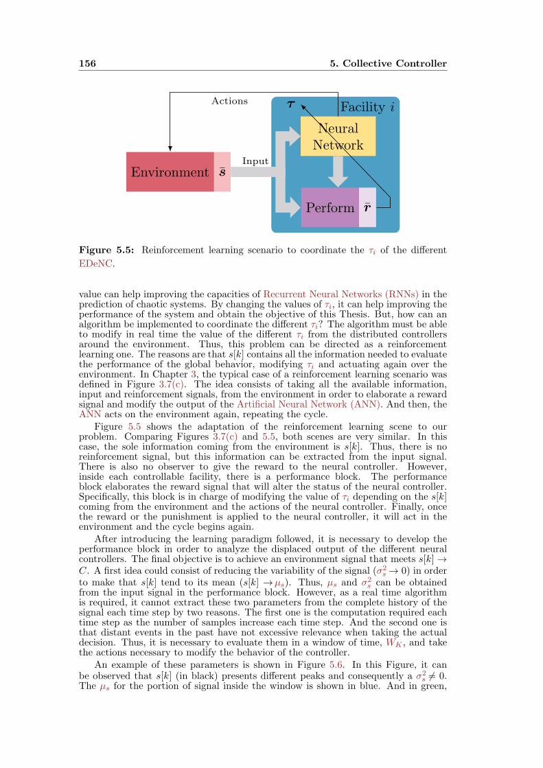
156 5. Collective Controller
Facility i
Environment s
Neural
Network
Perform r
Input
τActions
Figure 5.5: Reinforcement learning scenario to coordinate the τi of the different
EDeNC.
value can help improving the capacities of Recurrent Neural Networks (RNNs) in theprediction of chaotic systems. By changing the values of τi, it can help improving theperformance of the system and obtain the objective of this Thesis. But, how can analgorithm be implemented to coordinate the different τi? The algorithm must be ableto modify in real time the value of the different τi from the distributed controllersaround the environment. Thus, this problem can be directed as a reinforcementlearning one. The reasons are that s[k] contains all the information needed to evaluatethe performance of the global behavior, modifying τi and actuating again over theenvironment. In Chapter 3, the typical case of a reinforcement learning scenario wasdefined in Figure 3.7(c). The idea consists of taking all the available information,input and reinforcement signals, from the environment in order to elaborate a rewardsignal and modify the output of the Artificial Neural Network (ANN). And then, theANN acts on the environment again, repeating the cycle.
Figure 5.5 shows the adaptation of the reinforcement learning scene to ourproblem. Comparing Figures 3.7(c) and 5.5, both scenes are very similar. In thiscase, the sole information coming from the environment is s[k]. Thus, there is noreinforcement signal, but this information can be extracted from the input signal.There is also no observer to give the reward to the neural controller. However,inside each controllable facility, there is a performance block. The performanceblock elaborates the reward signal that will alter the status of the neural controller.Specifically, this block is in charge of modifying the value of τi depending on the s[k]coming from the environment and the actions of the neural controller. Finally, oncethe reward or the punishment is applied to the neural controller, it will act in theenvironment and the cycle begins again.
After introducing the learning paradigm followed, it is necessary to develop theperformance block in order to analyze the displaced output of the different neuralcontrollers. The final objective is to achieve an environment signal that meets s[k]→C. A first idea could consist of reducing the variability of the signal (σ2
s→ 0) in orderto make that s[k] tend to its mean (s[k] →µs). Thus, µs and σ2
s can be obtainedfrom the input signal in the performance block. However, as a real time algorithmis required, it cannot extract these two parameters from the complete history of thesignal each time step by two reasons. The first one is the computation required eachtime step as the number of samples increase each time step. And the second one isthat distant events in the past have not excessive relevance when taking the actualdecision. Thus, it is necessary to evaluate them in a window of time, WK , and takethe actions necessary to modify the behavior of the controller.
An example of these parameters is shown in Figure 5.6. In this Figure, it canbe observed that s[k] (in black) presents different peaks and consequently a σ2
s = 0.The µs for the portion of signal inside the window is shown in blue. And in green,
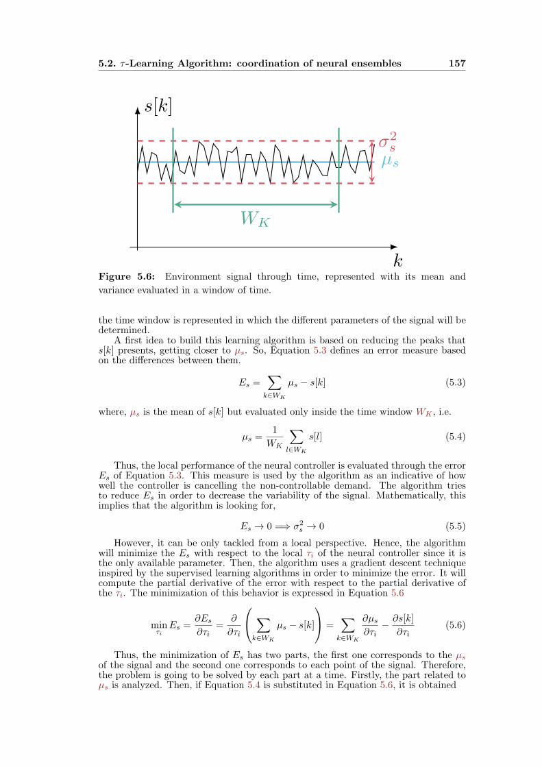
5.2. τ-Learning Algorithm: coordination of neural ensembles 157
µs
σ2
s
WK
k
s[k]
Figure 5.6: Environment signal through time, represented with its mean and
variance evaluated in a window of time.
the time window is represented in which the different parameters of the signal will bedetermined.
A first idea to build this learning algorithm is based on reducing the peaks thats[k] presents, getting closer to µs. So, Equation 5.3 defines an error measure basedon the differences between them.
Es =∑
k∈WK
µs − s[k] (5.3)
where, µs is the mean of s[k] but evaluated only inside the time window WK , i.e.
µs =1
WK
∑l∈WK
s[l] (5.4)
Thus, the local performance of the neural controller is evaluated through the errorEs of Equation 5.3. This measure is used by the algorithm as an indicative of howwell the controller is cancelling the non-controllable demand. The algorithm triesto reduce Es in order to decrease the variability of the signal. Mathematically, thisimplies that the algorithm is looking for,
Es → 0 =⇒ σ2s → 0 (5.5)
However, it can be only tackled from a local perspective. Hence, the algorithmwill minimize the Es with respect to the local τi of the neural controller since it isthe only available parameter. Then, the algorithm uses a gradient descent techniqueinspired by the supervised learning algorithms in order to minimize the error. It willcompute the partial derivative of the error with respect to the partial derivative ofthe τi. The minimization of this behavior is expressed in Equation 5.6
minτi
Es =∂Es
∂τi=
∂
∂τi
∑k∈WK
µs − s[k]
=∑
k∈WK
∂µs
∂τi− ∂s[k]
∂τi(5.6)
Thus, the minimization of Es has two parts, the first one corresponds to the µsof the signal and the second one corresponds to each point of the signal. Therefore,the problem is going to be solved by each part at a time. Firstly, the part related toµs is analyzed. Then, if Equation 5.4 is substituted in Equation 5.6, it is obtained
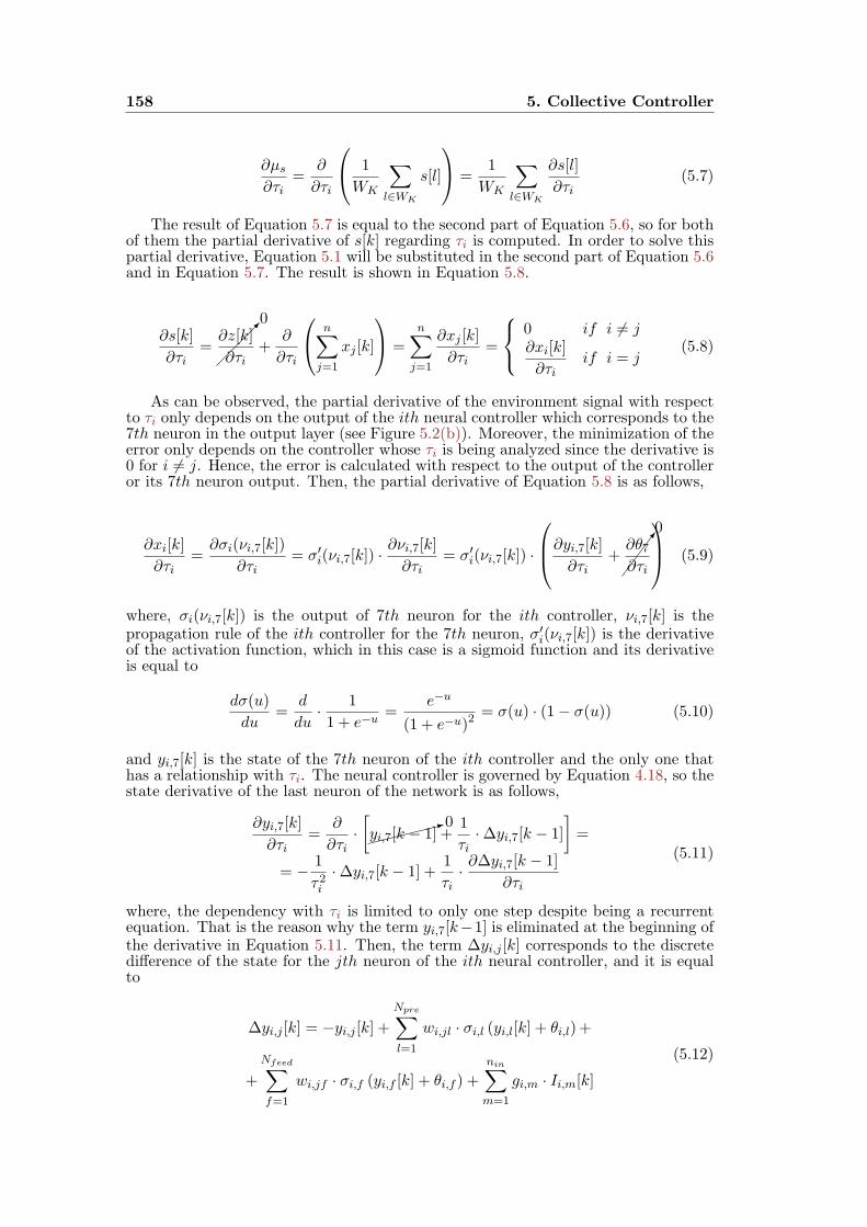
158 5. Collective Controller
∂µs
∂τi=
∂
∂τi
1
WK
∑l∈WK
s[l]
=1
WK
∑l∈WK
∂s[l]
∂τi(5.7)
The result of Equation 5.7 is equal to the second part of Equation 5.6, so for bothof them the partial derivative of s[k] regarding τi is computed. In order to solve thispartial derivative, Equation 5.1 will be substituted in the second part of Equation 5.6and in Equation 5.7. The result is shown in Equation 5.8.
∂s[k]
∂τi=
0
∂z[k]
∂τi+
∂
∂τi
n∑j=1
xj [k]
=
n∑j=1
∂xj [k]
∂τi=
0 if i = j∂xi[k]
∂τiif i = j
(5.8)
As can be observed, the partial derivative of the environment signal with respectto τi only depends on the output of the ith neural controller which corresponds to the7th neuron in the output layer (see Figure 5.2(b)). Moreover, the minimization of theerror only depends on the controller whose τi is being analyzed since the derivative is0 for i = j. Hence, the error is calculated with respect to the output of the controlleror its 7th neuron output. Then, the partial derivative of Equation 5.8 is as follows,
∂xi[k]
∂τi=
∂σi(νi,7[k])
∂τi= σ′
i(νi,7[k]) ·∂νi,7[k]
∂τi= σ′
i(νi,7[k]) ·
∂yi,7[k]
∂τi+
70
∂θ7∂τi
(5.9)
where, σi(νi,7[k]) is the output of 7th neuron for the ith controller, νi,7[k] is thepropagation rule of the ith controller for the 7th neuron, σ′
i(νi,7[k]) is the derivativeof the activation function, which in this case is a sigmoid function and its derivativeis equal to
dσ(u)
du=
d
du· 1
1 + e−u=
e−u
(1 + e−u)2= σ(u) · (1− σ(u)) (5.10)
and yi,7[k] is the state of the 7th neuron of the ith controller and the only one thathas a relationship with τi. The neural controller is governed by Equation 4.18, so thestate derivative of the last neuron of the network is as follows,
∂yi,7[k]
∂τi=
∂
∂τi·[
:0yi,7[k − 1] +
1
τi·∆yi,7[k − 1]
]=
= − 1
τ2i·∆yi,7[k − 1] +
1
τi· ∂∆yi,7[k − 1]
∂τi
(5.11)
where, the dependency with τi is limited to only one step despite being a recurrentequation. That is the reason why the term yi,7[k−1] is eliminated at the beginning ofthe derivative in Equation 5.11. Then, the term ∆yi,j [k] corresponds to the discretedifference of the state for the jth neuron of the ith neural controller, and it is equalto
∆yi,j [k] = −yi,j [k] +Npre∑l=1
wi,jl · σi,l (yi,l[k] + θi,l)+
+
Nfeed∑f=1
wi,jf · σi,f (yi,f [k] + θi,f ) +
nin∑m=1
gi,m · Ii,m[k]
(5.12)
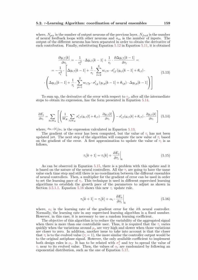
5.2. τ-Learning Algorithm: coordination of neural ensembles 159
where, Npre is the number of output neurons of the previous layer, Nfeed is the numberof neural feedback loops with other neurons and nin is the number of inputs. Theoutput of the different neurons has been separated in order to obtain the derivative ofeach contribution. Finally, substituting Equation 5.12 in Equation 5.11, it is obtained
∂yi,7[k]
∂τi= − 1
τ2i·∆yi,7[k − 1] +
1
τi· ∂∆yi,7[k − 1]
∂τi=
= − 1
τ2i·
[∆yi,7[k − 1] +
1
τi·
6∑l=3
wi,7l · σ′i,l (yi,l[k − 1] + θi,l) ·
·
∆yi,l[k − 1] +1
τi·
2∑p=1
wi,7p · σ′i,p (yi,p[k − 1] + θi,p) ·∆yi,p[k − 1]
(5.13)
To sum up, the derivative of the error with respect to τi, after all the intermediatesteps to obtain its expression, has the form presented in Equation 5.14.
∂Es
∂τi=∑
k∈WK
1
WK
∑l∈WK
σ′i,7(yi,7[l] + θi,7) ·
∂yi,7[l]
∂τi
− σ′i,7(yi,7[k] + θi,7) ·
∂yi,7[k]
∂τi
(5.14)
where, ∂yi,7[k]/∂τi is the expression calculated in Equation 5.13.The gradient of the error has been computed, but the value of τi has not been
updated yet. The next step of the algorithm will compute the new value of τi basedon the gradient of the error. A first approximation to update the value of τi is asfollows,
τi[k + 1] = τi[k] +∂Es
∂τi
∣∣∣∣k
(5.15)
As can be observed in Equation 5.15, there is a problem with this update and itis based on the nature of the neural controllers. All the τi are going to have the samevalue each time step and still there is no coordination between the different ensemblesof neural controllers. Then, a multiplier for the gradient of error can be used in orderto set the learning pace of τi. This technique is used in different supervised learningalgorithms to establish the growth pace of the parameters to adjust as shown inSection 3.5.1.1. Equation 5.16 shows this new τi update rule.
τi[k + 1] = τi[k] + αi ·∂Es
∂τi
∣∣∣∣k
(5.16)
where, αi is the learning rate of the gradient error for the ith neural controller.Normally, the learning rate in any supervised learning algorithm is a fixed number.However, in this case, it is necessary to use a random learning coefficient.
The objective of this algorithm is to reduce the variability of the aggregated signalwhen there is more than one controllable user. Thus, it is required that the τi variesquickly when the variations around µs are very high and slower when those variationsare closer to zero. In addition, another issue to take into account is that the closerthat τi is to the evolved value (τi= 1), the more similar the controller output would beto the original antiphase signal. However, the only available coefficient to implementboth design rules is αi. It has to be related with σ2
s and try to spread the value ofτi near to its evolved value. Then, the values of αi are randomized by following anexponential distribution, such as the one of Equation 5.17.

160 5. Collective Controller
Algorithm 1 High-level description of the τ -Learning Algorithm.
1: /* Initialize the environment */
2:∑
i∈n xi ← CTRNN ▷ n individuals with the same controller
3: z ← Power profile ▷ m non controllable individuals
4: for k ← 1, . . . ,K do
5: for all i ∈ n do
6: xi[k]← f(s[k − 1],y)
7: end for
8: s[k]← z[k] +∑
i∈n xi9: if k%WK == 0 then
10: Calculate µs, σ2s
11: for all i ∈ n do
12: Compute ∂Es/∂τi based on Equation 5.14
13: Obtain αi following Equation 5.17
14: Update τi based on Equation 5.16
15: Assure stability of the system
16: end for
17: end if
18: end for
αi(x, σ2s) =
σ2s · e−σ2
s ·x x ≥ 0,
0 x < 0.
where σ2s =
1
WK
∑l∈WK
s[l]
2
− µ2s
(5.17)
where, αi(x, σ2s) is the exponential probability function for the αi and whose mean is
located at σ2s , which is the variance of s[k] for WK . This distribution has been selected
because the higher probabilities are around the mean of the exponential distribution(in this case is σ2
s). So most of the τi are going to have a similar rate of change.Moreover, being the exponential distribution centered on σ2
s , αi will change with itsvalue. Fulfilling that αi will be lower as the σ2
s is being reduced, the values of τi willchange slowly, and vice versa.
To sum up, all the steps of the τ -Learning Algorithm (τLA) are gathered inAlgorithm 1. First of all, the environment is initialized with m non-controllableusers and the n controllable users. After that, the time starts and it will firstcalculate the output of each neural controller. Then, their responses are added tothe environment together with the non-controllable users. When the time is of thesame size as WK , then the environment status is evaluated. Therefore, it computesthe different measures to correct the behavior of the neural controllers and finally, itupdates the value of τi. Algorithm 1 has been tested in simulations. However, beforetesting the algorithm, it must be analyzed the stability of the system and the valuesthat τi can take.
5.2.1 Stability
Depending on the value of τi, there will be different stability behaviors. Thus, it isinteresting to analyze the values that τi can take in order to maintain the stability of

5.3. Simulation Results 161
the neural controllers. Each neural controller is governed by a system of differentialequations, in which each neuron is represented by Equation 4.15. However, Equation4.15 is simplified in order to analyze the effect of τi in the stability of the ith neuron.This simplification is as follows,
yi(t) = a · yi(t) + ui(t) (5.18)
where, a = − 1/τi and ui(t) is the rest of the terms of Equation 4.15, grouping togetherall the inputs to the neuron. In order to work with the neural controller, it is usedin discrete time. The discretization of Equation 5.18 is particularized for only onesample (∆k = 1) as it was done in Section 4.3.2.
yi[k]− yi[k −∆k]
∆k= a · yi[k] + ui[k] −→
∆k=1yi[k]− yi[k − 1] = a · yi[k] + ui[k] (5.19)
In order to analyze Equation 5.19, the Z-transform is used to pass from the discretetime to the complex frequency domain. The Z-transform is,
(1− a) · yi[k] = yi[k − 1] + ui[k]Z−→ (1− a)Yi(z) = z−1 · Yi(z) + Ui(z)
Hi(z) =Yi(z)
Ui(z)=
1
(1− a)− z−1
(5.20)
Finally, the stability of the neuron is given by the poles of the Hi(z), which arein the denominator D(Hi(z)). Thus, the system will be stable if the poles are insidethe unit circle of the complex plane. In this case, the Region of Convergence (ROC)is of the form,
|z| >∣∣∣∣ 1
1− a
∣∣∣∣ (5.21)
Hence, the denominator of the ROC condition must be greater than 0, in orderto meet and to assure the stability of the system. Then, substituting a by τi, thepossible values of τi are obtained in order not to disrupt the stability, as shown inEquation 5.22.
1− a ≥ 0a= − 1/τi−→ |τi| ≥ 1 (5.22)
The stability of the neuron depends on the value that τi can take. It can beconsidered that τi belongs to the positively defined axis since the sign is given by thestate of the neuron. Thus, in order to assure that the system is stable, τi∈ [1,+∞).And the τLA should assign values to τi respecting this condition.
5.3 Simulation Results
The environment is configured as in Figure 5.2(a) for the simulations of τLA. It hasbeen divided in m non-controllable users and n controllable users. Each one of the ncontrollable users have the same neural controller as the one of Figure 5.2(b). Theenvironment is governed by Equation 5.1 and it is necessary that τLA coordinatesthe n different users in order to smooth s[k]. In this case, for the evaluation of theτLA, only one input signal is used to simulate the non-controllable power profile.
The aggregated consumption of the m non-controllable individuals is nowmodelled as the aggregated consumption of a real grid. However, it is not exactlythe same signal (z7[k]), used in Section 4.5 and shown in Figure 4.3. A new signalhas been synthesized which consists of a sum of sinusoids. Five frequencies have beenselected, which are the ones with greater amplitude in the spectrum of Figure 4.3(b).
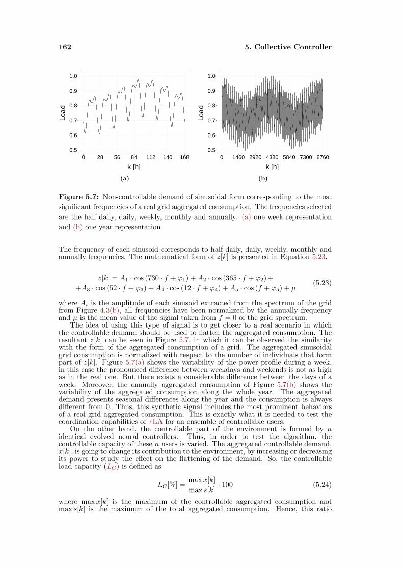
162 5. Collective Controller
0.5
0.6
0.7
0.8
0.9
1.0
0 28 56 84 112 140 168
k [h]
Load
(a)
0.5
0.6
0.7
0.8
0.9
1.0
0 1460 2920 4380 5840 7300 8760
k [h]
Load
(b)
Figure 5.7: Non-controllable demand of sinusoidal form corresponding to the most
significant frequencies of a real grid aggregated consumption. The frequencies selected
are the half daily, daily, weekly, monthly and annually. (a) one week representation
and (b) one year representation.
The frequency of each sinusoid corresponds to half daily, daily, weekly, monthly andannually frequencies. The mathematical form of z[k] is presented in Equation 5.23.
z[k] = A1 · cos (730 · f + φ1) +A2 · cos (365 · f + φ2)+
+A3 · cos (52 · f + φ3) +A4 · cos (12 · f + φ4) +A5 · cos (f + φ5) + µ(5.23)
where Ai is the amplitude of each sinusoid extracted from the spectrum of the gridfrom Figure 4.3(b), all frequencies have been normalized by the annually frequencyand µ is the mean value of the signal taken from f = 0 of the grid spectrum.
The idea of using this type of signal is to get closer to a real scenario in whichthe controllable demand should be used to flatten the aggregated consumption. Theresultant z[k] can be seen in Figure 5.7, in which it can be observed the similaritywith the form of the aggregated consumption of a grid. The aggregated sinusoidalgrid consumption is normalized with respect to the number of individuals that formpart of z[k]. Figure 5.7(a) shows the variability of the power profile during a week,in this case the pronounced difference between weekdays and weekends is not as highas in the real one. But there exists a considerable difference between the days of aweek. Moreover, the annually aggregated consumption of Figure 5.7(b) shows thevariability of the aggregated consumption along the whole year. The aggregateddemand presents seasonal differences along the year and the consumption is alwaysdifferent from 0. Thus, this synthetic signal includes the most prominent behaviorsof a real grid aggregated consumption. This is exactly what it is needed to test thecoordination capabilities of τLA for an ensemble of controllable users.
On the other hand, the controllable part of the environment is formed by nidentical evolved neural controllers. Thus, in order to test the algorithm, thecontrollable capacity of these n users is varied. The aggregated controllable demand,x[k], is going to change its contribution to the environment, by increasing or decreasingits power to study the effect on the flattening of the demand. So, the controllableload capacity (LC) is defined as
LC [%] =maxx[k]
max s[k]· 100 (5.24)
where maxx[k] is the maximum of the controllable aggregated consumption andmax s[k] is the maximum of the total aggregated consumption. Hence, this ratio

5.3. Simulation Results 163
relates the amount of controllable power to the total. Moreover, with the definitionof LC , it is also known the amount of power that the non-controllable users represent.
For the simulations, an amount of power is set for the controllable users throughLC and at the same time, the n size of controllable users is varied. Therefore, thetest will consist of analysing if the τLA is able to coordinate different ensembles ofneural controllers and if their self-organization is able to reduce the variability of thenon-controllable signal by obtaining a smooth s[k]. In the simulations, the percentageof LC varies from 0% to 100%. With this sweep of LC , it is analyzed the full range ofsituations that may occur in the environment, from an initial state at which there isno controllable demand (LC near 0%) until all the demand is controllable (LC near100%). Per each LC , the number of controllable users n is varied. The distribution ofthe number of individuals is not linear because it is necessary to test that τLA worksfor every population. Thus, it will be used a population set that grows exponentiallywhose values are n ∈ 1, 2, 5, 10, 25, 50, 100, 250, 500, 1000. The idea of this set ofindividuals is to increase the difficulty of coordination for the algorithm. The reasonis that for small populations the variations that individuals can introduce in theenvironment are smaller than the ones of bigger populations. So, simulations withfew individuals are easier to solve than the ones with bigger populations since lessinstabilities are present and fewer individuals need to coordinate.
The different simulation elements have just been described but the evaluationmethod has not been discussed yet. This method will consist of analyzing the globalbehavior of the environment through the status of s[k]. For this purpose, 3 figuresof merit are used: i) crest factor (Cf ), ii) load factor (Lf ) and iii) demand factor(Df ). In this case, all three parameters evaluate the form of the signal and assessits smoothness. Thus, the performance of the algorithm is based on how flattened iss[k]. The reason is that the coordination of all the individuals must reduce the signalvariability. The first evaluation coefficient was already used in the post-evaluation ofthe evolved neural controller. On the other hand, the other two evaluation coefficientsare used in a real grid context to evaluate its dimension with respect to the maximumload. These three parameters are as follows:
Crest factor (Cf ). It has been already defined in Section 4.5 and itsmathematical expression is gathered in Equation 4.31.
Load factor (Lf ). The second evaluation coefficient is based on the use ofthe resources from the grid. It measures the average consumption in a periodwith respect to the maximum consumption. Thus, this coefficient serves asa measure to verify that the designed capacity of an electrical grid meets thedemand. Equation 5.25 shows the mathematical expression of this ratio whichconsists of the average load divided by the peak load in a specified time period.
Lf =s[k]
speak
∣∣∣∣∣K
(5.25)
where, s[k] is the average environment signal in a period K and speak is themaximum of the environment signal in a given time period. The value of thisratio is less than or equal to 1. Typically, this coefficient has a value less than 1because the facilities never operate at full capacity for the duration of the entireperiod selected. The interpretation of this coefficient is that the closer Lf is to1, the more constant is the usage of the grid. On the other hand, low values ofLf show a demand profile in which occasionally high peaks appear. Thus, thebest value of Lf is closer to 1 and indicates that s[k] is flattened.
Demand factor (Df ). This is the last factor of the evaluation and it alsomeasures the use of the resources. Df expresses the relationship of the amountof consumed power relative to the maximum power available that could beconsumed in the grid. Thus, Df compares the maximum demand in a time

164 5. Collective Controller
period with respect to maximum consumption of the system:
Df =max s[k]
smax
∣∣∣∣K
(5.26)
where, max s[k] is the maximum of s[k] in the specified time period K and smaxis the maximum possible load of the system. This is a measure of the occupancyof the system and it is relevant when trying to design the amount of load thata system should be rated for. This factor is always less than or equal to 1. Thecloser Df is to 1, the greater the use of the system is. In this way, the systemwould not be oversized and the resources will be used constantly, having againa flattened consumption.
In the simulations, z[k] has been sampled every 15 minutes. The total length ofa simulation is 35040 samples, which is the time length of a year sampled every 15minutes. In addition, the size of WK has to be adjusted for the algorithm in order toevaluate the performance of the controller. The length of the chosen WK is of a day,because during this period s[k] presents various peaks and it is enough time for theensemble of neural controllers to be coordinated and flattened the aggregated s[k].Each experiment is repeated 30 times with different seeds to randomize the processand test if similar solutions can be obtained for different starting points. In addition,the sweep done in the LC goes from 0% to 100% in steps of 5% for the 10 sizesof individuals in the environment defined previously (from 1 to 1000). Then, 6300experiments are simulated to test the algorithm capabilities.
In the evaluation process, three figures of merit are defined. However, it wasnot mentioned the evaluation time in which they are going to be evaluated. Asobserved in Figure 5.7, there exist different peaks in the grid signal. Thus, the EDeNCeffectiveness is evaluated in order to cancel the main frequencies of the signal. Theevaluation of each coefficient is going to be done by using the daily, weekly, monthlyand annually periods. Hence, the controller behavior is tested during different timeperiods. The final result is the average of the number of times evaluated per timeperiod, i.e.
Cf,K =1
NK
∑i∈NK
Cf,i (5.27a) Lf,K =1
NK
∑i∈NK
Lf,i (5.27b)
Df,K =1
NK
∑i∈NK
Df,i (5.27c)
where K ∈ day, week,month, year and NK is the number of periods in which s[k]have been evaluated. Then, the average behavior of the controller is obtained alonga year for these three coefficients.
It has been explained all the different parameters and the evaluation assessmentthat take part in these simulations. However, simulations were carried out in twotype of environments depending on how s[k] is interpreted. The simulations havebeen divided in environment A (see Section 5.3.1) and environment B (see Section5.3.2). In the first one, the maximum consumed power is limited while in the secondone there will be no restriction. As in Chapter 4, all the simulations are done usingthe same hardware and software, neuralSim, already introduced. Thus, the resultsfor each environment are as follows.
5.3.1 Environment A: power constraints
In this environment, it is considered that the maximum power that can be consumedby all individuals is limited. So, the controllable users have to adapt their consumptionto the non-controllable demand in order not to consume more than the availablemaximum. With this environment, it is studied the adaptivity of the Evo-Devo NeuralController (EDeNC), and the ability of the τ -Learning Algorithm (τLA) to coordinate

5.3. Simulation Results 165
Day Week
Month Year
1.0
1.1
1.2
1.0
1.1
1.2
0 20 40 60 80 100 0 20 40 60 80 100
LC [%]
Cf
# n 12
510
2550
100250
5001000
Figure 5.8: Cf for environment A evaluated for four different periods of time: daily,
weekly, monthly and annually. The x-axis represents the variations of controllable
capacity (LC) and the color of each line represents a different size of controllable
users (#n).
different sizes of controllable ensembles for a given maximum power. This test wantsto cope with the case in which an existing grid is already working and new users areincluded without modifying the total power capabilities of the network.
A microgrid is a good example of this behavior which consists of a small communitywith some sources of local energy generation. In this microgrid, the generation isdesigned in order to supply the local demand. Thus, if new users are added to thismicrogrid, the local energy source would not be able to meet the demand and itwould be necessary to add more generation. However, if new users could adapt theirconsumption to the old ones, it would not be necessary to add more generation andthe use of the system would be improved.
In this case, the maximum of s[k] is limited to 1. For this purpose, the sumof the m non-controllable users and the n controllable ones must not exceed thislimit. Therefore, z[k] and xi[k] have been normalized to take values in the range[0, 1]. Moreover, under these conditions, there is no necessity to evolve again the bestneural controller obtained in Chapter 4. Thus, the chromosome used in each neuralcontroller for xi[k] is the one evolved previously.
The average crest factor, Cf , results are shown in Figure 5.8. The results havebeen separated for the four different periods of time in which s[k] is evaluated. Each
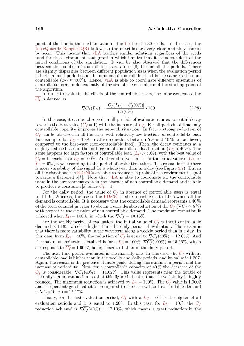
166 5. Collective Controller
point of the line is the median value of the Cf for the 30 seeds. In this case, theInterQuartile Range (IQR) is low, so the quartiles are very close and they cannotbe seen. This means that τLA reaches similar solutions regardless of the seedsused for the environment configuration which implies that it is independent of theinitial conditions of the simulation. It can be also observed that the differencesbetween the number of controllable users are negligible for all the periods. Thereare slightly disparities between different population sizes when the evaluation periodis high (annual period) and the amount of controllable load is the same as the non-controllable (LC ≈ 50%). Hence, τLA is able to coordinate different ensembles ofcontrollable users, independently of the size of the ensemble and the starting point ofthe algorithm.
In order to evaluate the effects of the controllable users, the improvement of theCf is defined as
∇Cf (LC) =|Cf (LC)− Cf (0%)|
Cf (0%)· 100 (5.28)
In this case, it can be observed in all periods of evaluation an exponential decaytowards the best value (Cf = 1) with the increase of LC . For all periods of time, anycontrollable capacity improves the network situation. In fact, a strong reduction ofCf can be observed in all the cases with relatively low fractions of controllable load.For example, for LC = 10%, relative reductions between 5% and 10% are achieved,compared to the base-case (non-controllable load). Then, the decay continues at aslightly reduced rate in the mid region of controllable load fraction (LC ≈ 40%). Thesame happens for high factors of controllable load (LC > 50%), with the best value ofCf = 1, reached for LC = 100%. Another observation is that the initial value of Cf forLC = 0% grows according to the period of evaluation taken. The reason is that thereis more variability of the signal for a whole year than in a day (see Figure 5.7). But inall the situations the EDeNCs are able to reduce the peaks of the environment signaltowards a flattened s[k]. Note that τLA is able to coordinate all the controllableusers in the environment even in the absence of non-controllable demand and is ableto produce a constant s[k] since Cf = 1.
For the daily period, the value of Cf in absence of controllable users is equalto 1.119. Whereas, the use of the EDeNC is able to reduce it to 1.005 when all thedemand is controllable. It is necessary that the controllable demand represents a 40%of the total demand in order to obtain a considerable reduction of the Cf (∇Cf ≈ 8%)with respect to the situation of non-controllable demand. The maximum reduction isachieved when LC = 100%, in which the ∇Cf = 10.16%.
For the weekly period of evaluation, the initial value of Cf without controllabledemand is 1.185, which is higher than the daily period of evaluation. The reason isthat there is more variability in the waveform along a weekly period than in a day. Inthis case, from LC = 40%, the reduction of Cf is equal to ∇Cf (40%) = 12.65%. And
the maximum reduction obtained is for a LC = 100%, ∇Cf (100%) = 15.55%, which
corresponds to Cf = 1.0007, being closer to 1 than in the daily period.
The next time period evaluated is the monthly one. In this case, the Cf withoutcontrollable load is higher than in the weekly and daily periods, and its value is 1.207.Again, the reason is the presence of more peaks during this evaluation period and theincrease of variability. Now, for a controllable capacity of 40% the decrease of theCf is considerable, ∇Cf (40%) = 14.02%. This value represents near the double ofthe daily period evaluation, so that this figure indicates that the variability is highlyreduced. The maximum reduction is achieved by LC = 100%. The Cf value is 1.0002and the percentage of reduction compared to the case without controllable demandis ∇Cf (100%) = 17.17%.
Finally, for the last evaluation period, Cf with a LC = 0% is the higher of all
evaluation periods and it is equal to 1.263. In this case, for LC = 40%, the Cf
reduction achieved is ∇Cf (40%) = 17.13%, which means a great reduction in the
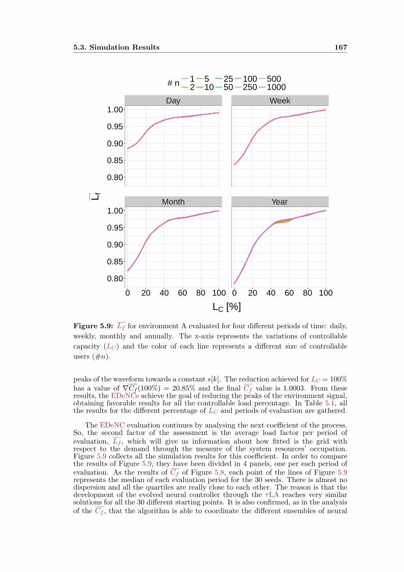
5.3. Simulation Results 167
Day Week
Month Year
0.80
0.85
0.90
0.95
1.00
0.80
0.85
0.90
0.95
1.00
0 20 40 60 80 100 0 20 40 60 80 100
LC [%]
L f# n 1
2510
2550
100250
5001000
Figure 5.9: Lf for environment A evaluated for four different periods of time: daily,
weekly, monthly and annually. The x-axis represents the variations of controllable
capacity (LC) and the color of each line represents a different size of controllable
users (#n).
peaks of the waveform towards a constant s[k]. The reduction achieved for LC = 100%has a value of ∇Cf (100%) = 20.85% and the final Cf value is 1.0003. From theseresults, the EDeNCs achieve the goal of reducing the peaks of the environment signal,obtaining favorable results for all the controllable load percentage. In Table 5.1, allthe results for the different percentage of LC and periods of evaluation are gathered.
The EDeNC evaluation continues by analysing the next coefficient of the process.So, the second factor of the assessment is the average load factor per period ofevaluation, Lf , which will give us information about how fitted is the grid withrespect to the demand through the measure of the system resources’ occupation.Figure 5.9 collects all the simulation results for this coefficient. In order to comparethe results of Figure 5.9, they have been divided in 4 panels, one per each period ofevaluation. As the results of Cf of Figure 5.8, each point of the lines of Figure 5.9represents the median of each evaluation period for the 30 seeds. There is almost nodispersion and all the quartiles are really close to each other. The reason is that thedevelopment of the evolved neural controller through the τLA reaches very similarsolutions for all the 30 different starting points. It is also confirmed, as in the analysisof the Cf , that the algorithm is able to coordinate the different ensembles of neural
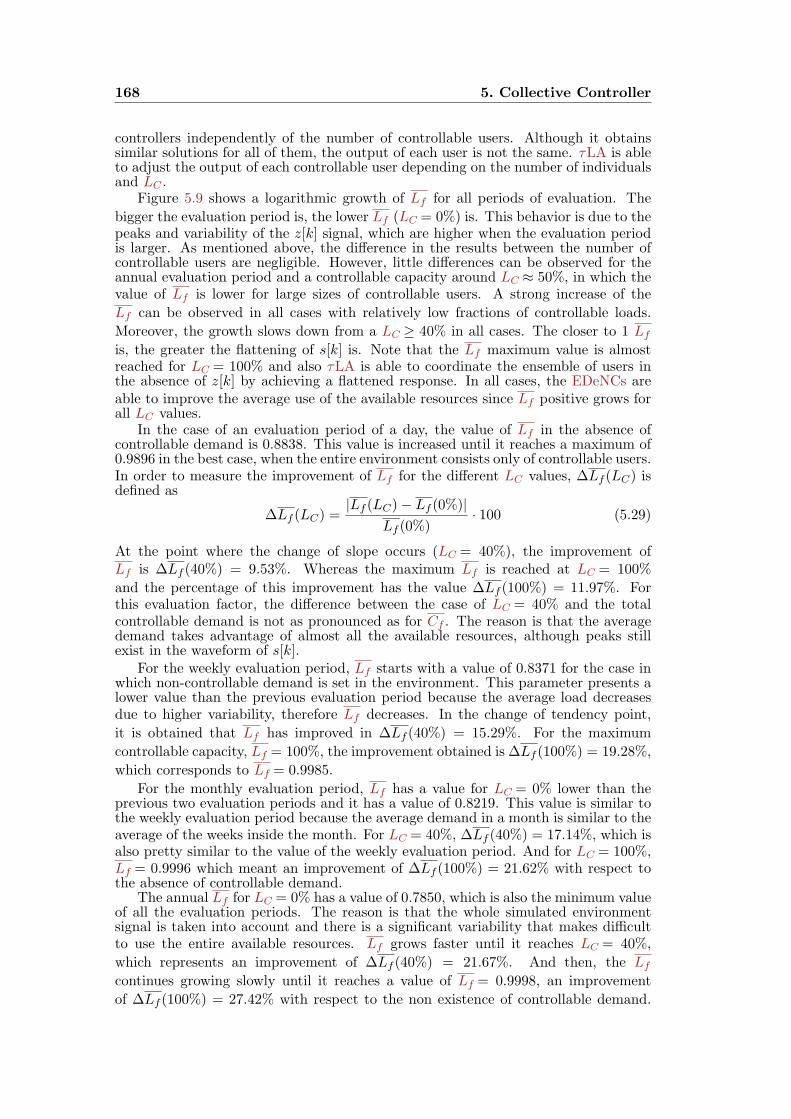
168 5. Collective Controller
controllers independently of the number of controllable users. Although it obtainssimilar solutions for all of them, the output of each user is not the same. τLA is ableto adjust the output of each controllable user depending on the number of individualsand LC .
Figure 5.9 shows a logarithmic growth of Lf for all periods of evaluation. The
bigger the evaluation period is, the lower Lf (LC = 0%) is. This behavior is due to thepeaks and variability of the z[k] signal, which are higher when the evaluation periodis larger. As mentioned above, the difference in the results between the number ofcontrollable users are negligible. However, little differences can be observed for theannual evaluation period and a controllable capacity around LC ≈ 50%, in which thevalue of Lf is lower for large sizes of controllable users. A strong increase of the
Lf can be observed in all cases with relatively low fractions of controllable loads.
Moreover, the growth slows down from a LC ≥ 40% in all cases. The closer to 1 Lf
is, the greater the flattening of s[k] is. Note that the Lf maximum value is almostreached for LC = 100% and also τLA is able to coordinate the ensemble of users inthe absence of z[k] by achieving a flattened response. In all cases, the EDeNCs areable to improve the average use of the available resources since Lf positive grows forall LC values.
In the case of an evaluation period of a day, the value of Lf in the absence ofcontrollable demand is 0.8838. This value is increased until it reaches a maximum of0.9896 in the best case, when the entire environment consists only of controllable users.In order to measure the improvement of Lf for the different LC values, ∆Lf (LC) isdefined as
∆Lf (LC) =|Lf (LC)− Lf (0%)|
Lf (0%)· 100 (5.29)
At the point where the change of slope occurs (LC = 40%), the improvement ofLf is ∆Lf (40%) = 9.53%. Whereas the maximum Lf is reached at LC = 100%
and the percentage of this improvement has the value ∆Lf (100%) = 11.97%. Forthis evaluation factor, the difference between the case of LC = 40% and the totalcontrollable demand is not as pronounced as for Cf . The reason is that the averagedemand takes advantage of almost all the available resources, although peaks stillexist in the waveform of s[k].
For the weekly evaluation period, Lf starts with a value of 0.8371 for the case inwhich non-controllable demand is set in the environment. This parameter presents alower value than the previous evaluation period because the average load decreasesdue to higher variability, therefore Lf decreases. In the change of tendency point,
it is obtained that Lf has improved in ∆Lf (40%) = 15.29%. For the maximum
controllable capacity, Lf = 100%, the improvement obtained is ∆Lf (100%) = 19.28%,
which corresponds to Lf = 0.9985.
For the monthly evaluation period, Lf has a value for LC = 0% lower than theprevious two evaluation periods and it has a value of 0.8219. This value is similar tothe weekly evaluation period because the average demand in a month is similar to theaverage of the weeks inside the month. For LC = 40%, ∆Lf (40%) = 17.14%, which isalso pretty similar to the value of the weekly evaluation period. And for LC = 100%,Lf = 0.9996 which meant an improvement of ∆Lf (100%) = 21.62% with respect tothe absence of controllable demand.
The annual Lf for LC = 0% has a value of 0.7850, which is also the minimum valueof all the evaluation periods. The reason is that the whole simulated environmentsignal is taken into account and there is a significant variability that makes difficultto use the entire available resources. Lf grows faster until it reaches LC = 40%,
which represents an improvement of ∆Lf (40%) = 21.67%. And then, the Lf
continues growing slowly until it reaches a value of Lf = 0.9998, an improvement
of ∆Lf (100%) = 27.42% with respect to the non existence of controllable demand.
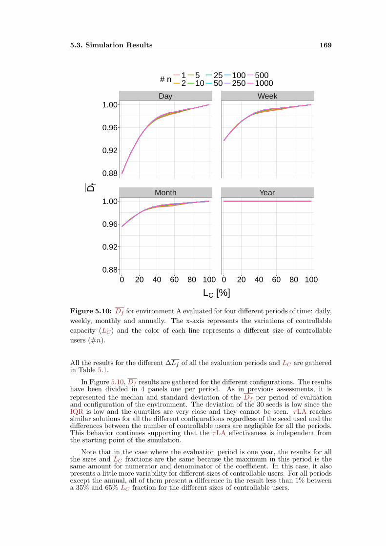
5.3. Simulation Results 169
Day Week
Month Year
0.88
0.92
0.96
1.00
0.88
0.92
0.96
1.00
0 20 40 60 80 100 0 20 40 60 80 100
LC [%]
Df
# n 12
510
2550
100250
5001000
Figure 5.10: Df for environment A evaluated for four different periods of time: daily,
weekly, monthly and annually. The x-axis represents the variations of controllable
capacity (LC) and the color of each line represents a different size of controllable
users (#n).
All the results for the different ∆Lf of all the evaluation periods and LC are gatheredin Table 5.1.
In Figure 5.10, Df results are gathered for the different configurations. The resultshave been divided in 4 panels one per period. As in previous assessments, it isrepresented the median and standard deviation of the Df per period of evaluationand configuration of the environment. The deviation of the 30 seeds is low since theIQR is low and the quartiles are very close and they cannot be seen. τLA reachessimilar solutions for all the different configurations regardless of the seed used and thedifferences between the number of controllable users are negligible for all the periods.This behavior continues supporting that the τLA effectiveness is independent fromthe starting point of the simulation.
Note that in the case where the evaluation period is one year, the results for allthe sizes and LC fractions are the same because the maximum in this period is thesame amount for numerator and denominator of the coefficient. In this case, it alsopresents a little more variability for different sizes of controllable users. For all periodsexcept the annual, all of them present a difference in the result less than 1% betweena 35% and 65% LC fraction for the different sizes of controllable users.

170 5. Collective Controller
Figure 5.10 shows a logarithmic growth as the results of Lf for daily, weekly
and monthly results. In this case, unlike the Lf results, the smaller the evaluation
period is, the bigger the value of Df for a LC = 0% is. This behavior is because theconsumption of most of the days is far from the maximum annual consumption. Inaddition, it can be observed a rapid growth for LC < 40%. This growth slows downuntil it reaches its maximum for LC = 100%. The best value for all the cases is 1,which means that the system is using all the resources during the entire evaluationperiod. With the EDeNCs, the system efficiency is increasing by using its full capacityand producing a flat signal that takes advantage of it.
For a daily evaluation period, Df is 0.876 for LC = 0%. Then, as the controllablecapacity increases in the environment this value grows until it reaches its maximum(Df = 1) for LC = 100%. As done before, a factor is defined that measures theimprovement of adding more LC . This coefficient has the following form,
∆Df (LC) =|Df (LC)−Df (0%)|
Df (0%)· 100 (5.30)
In the point at which the speed of growing reduces, the improvement achieved is∆Df (40%) = 11.05%. Whereas for the maximum value of the factor, s[k] was
improved in ∆Df (100%) = 13.72%. At LC = 100%, Df has reached its maximum
value so the ∆Df (100%) is the maximum value that s[k] could improve with the helpof the EDeNC.
The next evaluation period is the weekly period. In this case, Df begins with avalue of 0.936 for LC = 0%. It is bigger than the daily period since the peaks duringthe week are higher than for one day. At a LC = 40%, the EDeNC have improved thefactor in ∆Df (40%) = 5.56%, which is lower than the previous value since it starts
closer to the maximum value. With LC = 100%, it is obtained a Df = 1 with an
improvement of ∆Df (100%) = 6.82% with respect to the case with no controllableload. As can be observed, the improvement for the best LC is similar to a LC = 40%.The reason is that the maximum peak of the week is closer to the maximum ofthe system, but the algorithm continuous improving this value until its maximum isreached.
The last period analysed is the monthly period, since the improvement of theannual period is inexistent as it always uses the maximum capacity of the system. Abigger value of Df is achieved for LC = 0% which is equal to 0.955. It also reaches
the maximum value of Df = 1 for LC = 100%, which means a maximum improvement
of ∆Df (100%) = 4.76% (lower than the previous periods due to being close to the
maximum). Meanwhile, for LC = 40%, the algorithm achieves ∆Df (40%) = 3.89%which is closed to the maximum possible value of improvement. By following the samereasoning as with the weekly period, the maximum peak found during the evaluationof a month is closer to maximum of the system, so the Df is closer to 1. The rest ofthe results are summarized in Table 5.1 for all the periods and LC .
One last result that it is going to be analyzed is how flat the environment signalis for the different controllable fractions, LC . In order to do this analysis, therepresentation of the load duration curve explained in Section 2.1.5 is used. Thisrepresentation consists of sorting decreasingly the consumption along the 8760 h ofa year. Thus, the maximum consumption of the year is at 0 h and the minimumis located at 8759 h. And in order to compare them, the load is normalized by themaximum load available in the environment, i.e. the sum of the maximum load thateach user can consume. Figure 5.11 shows the different load duration curves fordifferent controllable fractions.
In view of these results, it can be concluded that the use of any controllabledemand will improve the grid status since the variability of s[k] is reduced (the valueof the slope decreases) and also the maximum consumption of the grid is reducedas LC grows. Another finding that emerges from these results is that the demand
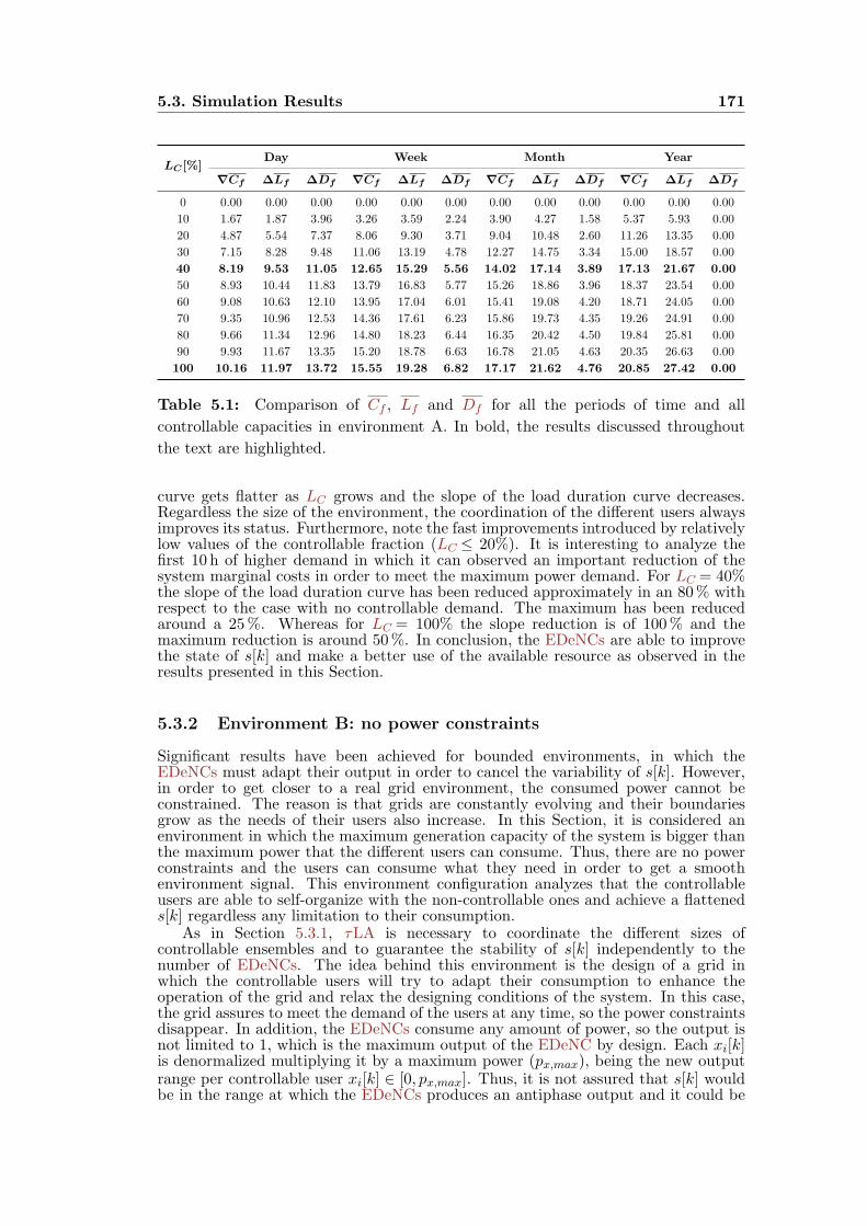
5.3. Simulation Results 171
LC[%]Day Week Month Year
∇Cf ∆Lf ∆Df ∇Cf ∆Lf ∆Df ∇Cf ∆Lf ∆Df ∇Cf ∆Lf ∆Df
0 0.00 0.00 0.00 0.00 0.00 0.00 0.00 0.00 0.00 0.00 0.00 0.00
10 1.67 1.87 3.96 3.26 3.59 2.24 3.90 4.27 1.58 5.37 5.93 0.00
20 4.87 5.54 7.37 8.06 9.30 3.71 9.04 10.48 2.60 11.26 13.35 0.00
30 7.15 8.28 9.48 11.06 13.19 4.78 12.27 14.75 3.34 15.00 18.57 0.00
40 8.19 9.53 11.05 12.65 15.29 5.56 14.02 17.14 3.89 17.13 21.67 0.00
50 8.93 10.44 11.83 13.79 16.83 5.77 15.26 18.86 3.96 18.37 23.54 0.00
60 9.08 10.63 12.10 13.95 17.04 6.01 15.41 19.08 4.20 18.71 24.05 0.00
70 9.35 10.96 12.53 14.36 17.61 6.23 15.86 19.73 4.35 19.26 24.91 0.00
80 9.66 11.34 12.96 14.80 18.23 6.44 16.35 20.42 4.50 19.84 25.81 0.00
90 9.93 11.67 13.35 15.20 18.78 6.63 16.78 21.05 4.63 20.35 26.63 0.00
100 10.16 11.97 13.72 15.55 19.28 6.82 17.17 21.62 4.76 20.85 27.42 0.00
Table 5.1: Comparison of Cf , Lf and Df for all the periods of time and all
controllable capacities in environment A. In bold, the results discussed throughout
the text are highlighted.
curve gets flatter as LC grows and the slope of the load duration curve decreases.Regardless the size of the environment, the coordination of the different users alwaysimproves its status. Furthermore, note the fast improvements introduced by relativelylow values of the controllable fraction (LC ≤ 20%). It is interesting to analyze thefirst 10 h of higher demand in which it can observed an important reduction of thesystem marginal costs in order to meet the maximum power demand. For LC = 40%the slope of the load duration curve has been reduced approximately in an 80% withrespect to the case with no controllable demand. The maximum has been reducedaround a 25%. Whereas for LC = 100% the slope reduction is of 100% and themaximum reduction is around 50%. In conclusion, the EDeNCs are able to improvethe state of s[k] and make a better use of the available resource as observed in theresults presented in this Section.
5.3.2 Environment B: no power constraints
Significant results have been achieved for bounded environments, in which theEDeNCs must adapt their output in order to cancel the variability of s[k]. However,in order to get closer to a real grid environment, the consumed power cannot beconstrained. The reason is that grids are constantly evolving and their boundariesgrow as the needs of their users also increase. In this Section, it is considered anenvironment in which the maximum generation capacity of the system is bigger thanthe maximum power that the different users can consume. Thus, there are no powerconstraints and the users can consume what they need in order to get a smoothenvironment signal. This environment configuration analyzes that the controllableusers are able to self-organize with the non-controllable ones and achieve a flatteneds[k] regardless any limitation to their consumption.
As in Section 5.3.1, τLA is necessary to coordinate the different sizes ofcontrollable ensembles and to guarantee the stability of s[k] independently to thenumber of EDeNCs. The idea behind this environment is the design of a grid inwhich the controllable users will try to adapt their consumption to enhance theoperation of the grid and relax the designing conditions of the system. In this case,the grid assures to meet the demand of the users at any time, so the power constraintsdisappear. In addition, the EDeNCs consume any amount of power, so the output isnot limited to 1, which is the maximum output of the EDeNC by design. Each xi[k]is denormalized multiplying it by a maximum power (px,max), being the new outputrange per controllable user xi[k] ∈ [0, px,max]. Thus, it is not assured that s[k] wouldbe in the range at which the EDeNCs produces an antiphase output and it could be
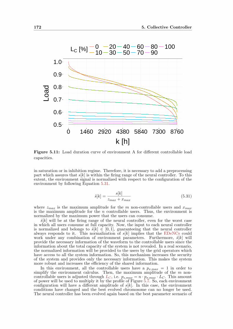
172 5. Collective Controller
0.5
0.6
0.7
0.8
0.9
1.0
0 1460 2920 4380 5840 7300 8760
k [h]
Load
LC [%] 010
2030
4050
6070
8090
100
Figure 5.11: Load duration curve of environment A for different controllable load
capacities.
in saturation or in inhibition regime. Therefore, it is necessary to add a preprocessingpart which assures that s[k] is within the firing range of the neural controller. To thisextent, the environment signal is normalized with respect to the configuration of theenvironment by following Equation 5.31.
s[k] =s[k]
zmax + xmax(5.31)
where zmax is the maximum amplitude for the m non-controllable users and xmaxis the maximum amplitude for the n controllable users. Thus, the environment isnormalized by the maximum power that the users can consume.
s[k] will be at the firing range of the neural controller, even for the worst casein which all users consume at full capacity. Now, the input to each neural controlleris normalized and belongs to s[k] ∈ [0, 1], guaranteeing that the neural controlleralways responds to it. This normalization of s[k] implies that the EDeNCs couldwork under any combination of environment parameters. Furthermore, s[k] willprovide the necessary information of the waveform to the controllable users since theinformation about the total capacity of the system is not revealed. In a real scenario,the normalized information will be provided to the users by the grid operators whichhave access to all the system information. So, this mechanism increases the securityof the system and provides only the necessary information. This makes the systemmore robust and increases the efficiency of the shared information.
In this environment, all the controllable users have a px,max = 1 in order tosimplify the environment calculus. Then, the maximum amplitude of the m non-controllable users is adjusted through LC , i.e. pz,max = n · px,max · LC . This amountof power will be used to multiply it by the profile of Figure 5.7. So, each environmentconfiguration will have a different amplitude of s[k]. In this case, the environmentconditions have changed and the best evolved chromosome can no longer be used.The neural controller has been evolved again based on the best parameter scenario of
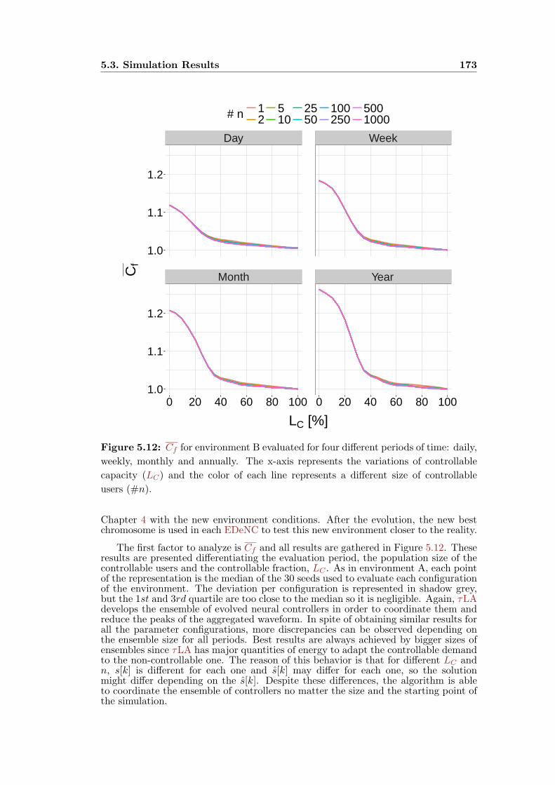
5.3. Simulation Results 173
Day Week
Month Year
1.0
1.1
1.2
1.0
1.1
1.2
0 20 40 60 80 100 0 20 40 60 80 100
LC [%]
Cf
# n 12
510
2550
100250
5001000
Figure 5.12: Cf for environment B evaluated for four different periods of time: daily,
weekly, monthly and annually. The x-axis represents the variations of controllable
capacity (LC) and the color of each line represents a different size of controllable
users (#n).
Chapter 4 with the new environment conditions. After the evolution, the new bestchromosome is used in each EDeNC to test this new environment closer to the reality.
The first factor to analyze is Cf and all results are gathered in Figure 5.12. Theseresults are presented differentiating the evaluation period, the population size of thecontrollable users and the controllable fraction, LC . As in environment A, each pointof the representation is the median of the 30 seeds used to evaluate each configurationof the environment. The deviation per configuration is represented in shadow grey,but the 1st and 3rd quartile are too close to the median so it is negligible. Again, τLAdevelops the ensemble of evolved neural controllers in order to coordinate them andreduce the peaks of the aggregated waveform. In spite of obtaining similar results forall the parameter configurations, more discrepancies can be observed depending onthe ensemble size for all periods. Best results are always achieved by bigger sizes ofensembles since τLA has major quantities of energy to adapt the controllable demandto the non-controllable one. The reason of this behavior is that for different LC andn, s[k] is different for each one and s[k] may differ for each one, so the solutionmight differ depending on the s[k]. Despite these differences, the algorithm is ableto coordinate the ensemble of controllers no matter the size and the starting point ofthe simulation.

174 5. Collective Controller
At the view of these results, it can be concluded that the inclusion of controllabledemand in the environment improves the waveform of the environment signal, makingit more constant as LC grows. This appreciation is observed for any of the evaluationperiods since the Cf is always reduced. In Figure 5.12, an exponential decay is
observed for all evaluation periods towards Cf = 1 as LC increases. It is also observedthat for LC ≤ 10%, the decay is slow. Then, it changes rapidly until it reaches aLC = 35%. And again the decay slows down until the best value of Cf is achieved forLC = 100%. In this case, the point at which the decay changes significantly is achievedbefore than in environment A. This is a positive effect because it indicates that thegreatest benefits are obtained at low LC , i.e. moderate investments. Moreover, theCf starting point grows with the evaluation period, since the variability of the signalalso increases. As in environment A, τLA is able to coordinate the EDeNC ensembleeven in the absence of z[k] and achieves a Cf = 1.
In order to detail the performance of the EDeNCs, the results of Figure 5.12 aredescribed as follows. For the case with LC = 0% in the daily period, the Cf value is
equal to 1.119, which is the same value as in environment A. The reason is that Cf isa waveform factor and it is independent of the scale. The application of τLA for theensemble coordination is able to obtain a Cf = 1.005, which is also the same valueas in environment A. So, Equation 5.28 will give the same amount of improvementof Cf , ∇Cf (100%) = 10.16%. However, at the point of change of slope LC = 35%,
a value of ∇Cf (35%) = 8.07% is obtained which is greater than in Environment Aunder the same percentage of controllability percentage. Therefore in both cases, thealgorithm has developed the evolved neural controller to the minimum Cf possible.
The same behavior can be observed for a weekly period of evaluation. At thepoint LC = 0%, the Cf obtained has a value of 1.185. Then, for LC = 35%, the
improvement of Cf is ∇Cf (35%) = 12.71%. s[k] is almost flattened at this point, itonly needs a small percentage to get its response as flatten as possible. Finally, themaximum reduction of Cf is achieved for LC = 100% and has a value of 1.001. This
value means an improvement of the waveform of ∇Cf (100%) = 15.55%.The next period evaluated is the monthly one. At this period, the starting point
of Cf is bigger than the previous ones because the variability of the signal is also
increased since more peaks of s[k] are evaluated. The value of Cf for LC = 0% is1.208. With the increase of LC , this value is reduced and at a controllable capacityof 35%, this reduction has a value of ∇Cf (35%) = 13.92%. The maximum reduction
is achieved by LC = 100%, the value of the Cf is 1.0002 and the reduction of the Cf
is of ∇Cf (100%) = 17.17%.Finally, the last evaluation of the environment is done by taking into account the
annual period signal. For this period, Cf has the biggest value due to the variability
of the signal. At a LC = 0%, the Cf has a value of 1.263. Then, Cf is reduced asthe controllability of the system grows. So, for the point which the slope changes itsspeed, LC = 35%, an improvement of ∇Cf (35%) = 16.52% is achieved. For this valueof LC , the s[k] has smoothed almost all the peaks presented in its waveform. Thereduction of Cf continues growing until it reaches a value of 1.0001, which means an
improvement of ∇Cf (100%) = 20.82%. For all the periods, the results at LC = 100%are very similar, meaning that the coordination algorithm found the best possiblesolution to flatten s[k]. All the reduction results are gathered in Table 5.2 to see inmore detail the values obtained for each controllability fraction.
The next evaluation coefficient is Lf which will report information about howgood the average occupation of the environment is with respect to the maximumconsumption. It is a measure of how well the grid meets its demand. Figure 5.13shows all the result for the assessment of this factor. Note that, the closer Lf is to 1,the more constant is s[k]. The four evaluation periods are represented in a differentpanel of Figure 5.13. All the points are the median representation of evaluating
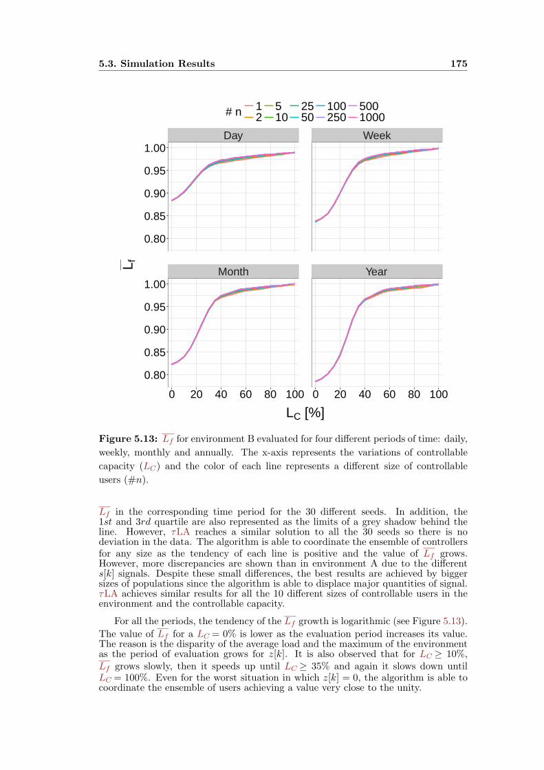
5.3. Simulation Results 175
Day Week
Month Year
0.80
0.85
0.90
0.95
1.00
0.80
0.85
0.90
0.95
1.00
0 20 40 60 80 100 0 20 40 60 80 100
LC [%]
L f# n 1
2510
2550
100250
5001000
Figure 5.13: Lf for environment B evaluated for four different periods of time: daily,
weekly, monthly and annually. The x-axis represents the variations of controllable
capacity (LC) and the color of each line represents a different size of controllable
users (#n).
Lf in the corresponding time period for the 30 different seeds. In addition, the1st and 3rd quartile are also represented as the limits of a grey shadow behind theline. However, τLA reaches a similar solution to all the 30 seeds so there is nodeviation in the data. The algorithm is able to coordinate the ensemble of controllersfor any size as the tendency of each line is positive and the value of Lf grows.However, more discrepancies are shown than in environment A due to the differents[k] signals. Despite these small differences, the best results are achieved by biggersizes of populations since the algorithm is able to displace major quantities of signal.τLA achieves similar results for all the 10 different sizes of controllable users in theenvironment and the controllable capacity.
For all the periods, the tendency of the Lf growth is logarithmic (see Figure 5.13).
The value of Lf for a LC = 0% is lower as the evaluation period increases its value.The reason is the disparity of the average load and the maximum of the environmentas the period of evaluation grows for z[k]. It is also observed that for LC ≥ 10%,Lf grows slowly, then it speeds up until LC ≥ 35% and again it slows down untilLC = 100%. Even for the worst situation in which z[k] = 0, the algorithm is able tocoordinate the ensemble of users achieving a value very close to the unity.
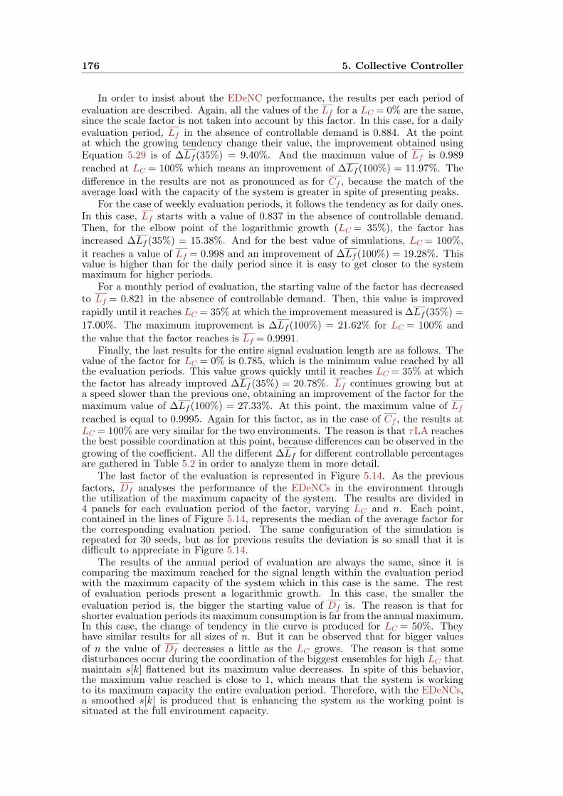
176 5. Collective Controller
In order to insist about the EDeNC performance, the results per each period ofevaluation are described. Again, all the values of the Lf for a LC = 0% are the same,since the scale factor is not taken into account by this factor. In this case, for a dailyevaluation period, Lf in the absence of controllable demand is 0.884. At the pointat which the growing tendency change their value, the improvement obtained usingEquation 5.29 is of ∆Lf (35%) = 9.40%. And the maximum value of Lf is 0.989
reached at LC = 100% which means an improvement of ∆Lf (100%) = 11.97%. The
difference in the results are not as pronounced as for Cf , because the match of theaverage load with the capacity of the system is greater in spite of presenting peaks.
For the case of weekly evaluation periods, it follows the tendency as for daily ones.In this case, Lf starts with a value of 0.837 in the absence of controllable demand.Then, for the elbow point of the logarithmic growth (LC = 35%), the factor hasincreased ∆Lf (35%) = 15.38%. And for the best value of simulations, LC = 100%,
it reaches a value of Lf = 0.998 and an improvement of ∆Lf (100%) = 19.28%. Thisvalue is higher than for the daily period since it is easy to get closer to the systemmaximum for higher periods.
For a monthly period of evaluation, the starting value of the factor has decreasedto Lf = 0.821 in the absence of controllable demand. Then, this value is improved
rapidly until it reaches LC = 35% at which the improvement measured is ∆Lf (35%) =
17.00%. The maximum improvement is ∆Lf (100%) = 21.62% for LC = 100% and
the value that the factor reaches is Lf = 0.9991.Finally, the last results for the entire signal evaluation length are as follows. The
value of the factor for LC = 0% is 0.785, which is the minimum value reached by allthe evaluation periods. This value grows quickly until it reaches LC = 35% at whichthe factor has already improved ∆Lf (35%) = 20.78%. Lf continues growing but ata speed slower than the previous one, obtaining an improvement of the factor for themaximum value of ∆Lf (100%) = 27.33%. At this point, the maximum value of Lf
reached is equal to 0.9995. Again for this factor, as in the case of Cf , the results atLC = 100% are very similar for the two environments. The reason is that τLA reachesthe best possible coordination at this point, because differences can be observed in thegrowing of the coefficient. All the different ∆Lf for different controllable percentagesare gathered in Table 5.2 in order to analyze them in more detail.
The last factor of the evaluation is represented in Figure 5.14. As the previousfactors, Df analyses the performance of the EDeNCs in the environment throughthe utilization of the maximum capacity of the system. The results are divided in4 panels for each evaluation period of the factor, varying LC and n. Each point,contained in the lines of Figure 5.14, represents the median of the average factor forthe corresponding evaluation period. The same configuration of the simulation isrepeated for 30 seeds, but as for previous results the deviation is so small that it isdifficult to appreciate in Figure 5.14.
The results of the annual period of evaluation are always the same, since it iscomparing the maximum reached for the signal length within the evaluation periodwith the maximum capacity of the system which in this case is the same. The restof evaluation periods present a logarithmic growth. In this case, the smaller theevaluation period is, the bigger the starting value of Df is. The reason is that forshorter evaluation periods its maximum consumption is far from the annual maximum.In this case, the change of tendency in the curve is produced for LC = 50%. Theyhave similar results for all sizes of n. But it can be observed that for bigger valuesof n the value of Df decreases a little as the LC grows. The reason is that somedisturbances occur during the coordination of the biggest ensembles for high LC thatmaintain s[k] flattened but its maximum value decreases. In spite of this behavior,the maximum value reached is close to 1, which means that the system is workingto its maximum capacity the entire evaluation period. Therefore, with the EDeNCs,a smoothed s[k] is produced that is enhancing the system as the working point issituated at the full environment capacity.
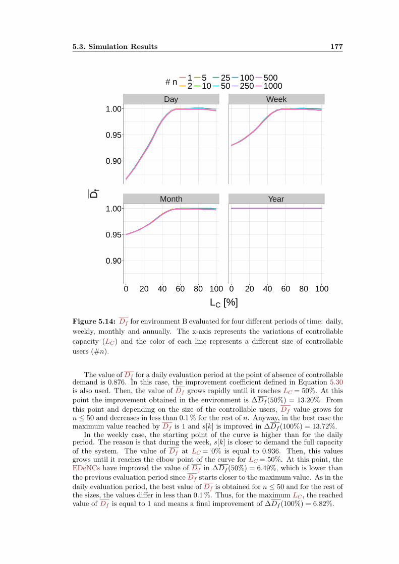
5.3. Simulation Results 177
Day Week
Month Year
0.90
0.95
1.00
0.90
0.95
1.00
0 20 40 60 80 100 0 20 40 60 80 100
LC [%]
Df
# n 12
510
2550
100250
5001000
Figure 5.14: Df for environment B evaluated for four different periods of time: daily,
weekly, monthly and annually. The x-axis represents the variations of controllable
capacity (LC) and the color of each line represents a different size of controllable
users (#n).
The value ofDf for a daily evaluation period at the point of absence of controllabledemand is 0.876. In this case, the improvement coefficient defined in Equation 5.30is also used. Then, the value of Df grows rapidly until it reaches LC = 50%. At this
point the improvement obtained in the environment is ∆Df (50%) = 13.20%. From
this point and depending on the size of the controllable users, Df value grows forn ≤ 50 and decreases in less than 0.1% for the rest of n. Anyway, in the best case themaximum value reached by Df is 1 and s[k] is improved in ∆Df (100%) = 13.72%.
In the weekly case, the starting point of the curve is higher than for the dailyperiod. The reason is that during the week, s[k] is closer to demand the full capacityof the system. The value of Df at LC = 0% is equal to 0.936. Then, this valuesgrows until it reaches the elbow point of the curve for LC = 50%. At this point, theEDeNCs have improved the value of Df in ∆Df (50%) = 6.49%, which is lower than
the previous evaluation period since Df starts closer to the maximum value. As in the
daily evaluation period, the best value of Df is obtained for n ≤ 50 and for the rest ofthe sizes, the values differ in less than 0.1%. Thus, for the maximum LC , the reachedvalue of Df is equal to 1 and means a final improvement of ∆Df (100%) = 6.82%.

178 5. Collective Controller
LC[%]Day Week Month Year
∇Cf ∆Lf ∆Df ∇Cf ∆Lf ∆Df ∇Cf ∆Lf ∆Df ∇Cf ∆Lf ∆Df
0 0.00 0.00 0.00 0.00 0.00 0.00 0.00 0.00 0.00 0.00 0.00 0.00
10 1.86 2.14 0.15 1.91 2.24 0.00 1.89 2.24 0.00 1.82 2.19 0.00
20 5.00 5.78 1.53 6.32 7.41 0.02 6.32 7.42 0.00 6.17 7.30 0.00
30 7.48 8.68 8.67 11.53 13.82 3.80 12.52 15.12 2.62 14.63 18.09 0.00
35 8.07 9.40 10.40 12.71 15.38 4.72 13.92 17.00 3.26 16.52 20.78 0.00
40 8.44 9.85 11.75 13.47 16.39 5.51 14.85 18.29 3.81 17.86 22.77 0.00
50 8.88 10.38 13.20 14.20 17.40 6.49 15.78 19.60 4.52 19.31 24.99 0.00
60 9.21 10.79 13.53 14.59 17.93 6.71 16.20 20.21 4.68 19.84 25.82 0.00
70 9.50 11.14 13.64 14.89 18.35 6.78 16.51 20.66 4.73 20.18 26.35 0.00
80 9.75 11.45 13.49 15.14 18.70 6.63 16.75 21.01 4.59 20.40 26.69 0.00
90 9.97 11.73 13.48 15.36 19.01 6.61 16.97 21.32 4.57 20.61 27.00 0.00
100 10.16 11.97 13.72 15.55 19.28 6.82 17.17 21.62 4.76 20.82 27.33 0.00
Table 5.2: Comparison of Cf , Lf and Df for all the periods of time and all
controllable capacities in environment B. In bold, the results discussed throughout
the text are highlighted.
The Df for the monthly evaluation period at LC = 0% has a value of 0.954.
Like the previous periods, Df presents the same behavior for the different sizes of
controllable users. It reaches a maximum value of Df = 1 for LC = 100%, which
means a maximum improvement of ∆Df (100%) = 4.52%. Whereas at the point
of tendency change LC = 50%, the algorithm achieves ∆Df (50%) = 4.76% quitenear to the maximum improvement. As for the previous coefficients, the resultsare very similar to the two environments, although the tendencies in the graphicalrepresentations differ. For all the periods and LC , the results are collected in Table5.2.
During the evaluation assessment of environment B, little differences have beenfound with respect to the results of environment A. Despite the difference in scale,τLA is able to found an optimum working point in all situations. Thus, the ensembleof evolved neural controllers is coordinated in order to flatten the response of s[k].However, some differences are appreciated as the tendencies and the different Cf , Lf
and Df curves present different forms. In addition, the last result of the assessment isthe flatness of the environment through its load duration curve. Figure 5.15 representsthe load duration curve for different percentage of controllable users. The curves havebeen normalized in order to compare them. In this case, τLA has reached differentsolutions than the ones obtained in Figure 5.11 for environment A. This confirms thatτLA is able to coordinate the ensemble of individuals searching for the best solutionto flatten s[k].
As stated before, the inclusion of any percentage of controllable demand improvesthe behavior of the system and reduces the variability of the grid. The slope of thecurves in Figure 5.15 is reduced as LC grows and gets flatter with the increasingcontrollable demand. It can be also observed how the maximum consumption ofthe system is reduced since the system efficiency increases with flatness of the gridenvironment. Regardless the size of the environment, the coordination of the differentusers always improves its status. As in environment A, it can be observed the fastimprovements introduced by relatively low values of the controllable fraction (LC ≤20%). And the analysis of the higher demand for the first 10 h leads to an importantreduction of the system marginal costs in order to meet the maximum power demand.To put some numbers to Figure 5.15, in the case for LC = 30%, the slope of the curvehas been reduced in a 81.60% with respect to the case of LC = 0% and the maximumconsumption of the environment has been reduced in a 28.93%. For the maximumcontrollable capacity (LC = 100%), the curve is constant, the reduction of the slope
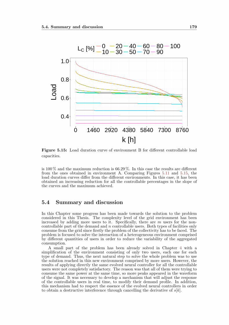
5.4. Summary and discussion 179
0.4
0.6
0.8
1.0
0 1460 2920 4380 5840 7300 8760
k [h]
Load
LC [%] 010
2030
4050
6070
8090
100
Figure 5.15: Load duration curve of environment B for different controllable load
capacities.
is 100% and the maximum reduction is 66.29%. In this case the results are differentfrom the ones obtained in environment A. Comparing Figures 5.11 and 5.15, theload duration curves differ from the different environments. In this case, it has beenobtained an increasing reduction for all the controllable percentages in the slope ofthe curves and the maximum achieved.
5.4 Summary and discussion
In this Chapter some progress has been made towards the solution to the problemconsidered in this Thesis. The complexity level of the grid environment has beenincreased by adding more users to it. Specifically, there are m users for the non-controllable part of the demand and n controllable users. Both types of facilities onlyconsume from the grid since firstly the problem of the collectivity has to be faced. Theproblem is focused to solve the interaction of a heterogeneous environment comprisedby different quantities of users in order to reduce the variability of the aggregatedconsumption.
A small part of the problem has been already solved in Chapter 4 with asimplification of the environment consisting of only two users, each one for eachtype of demand. Thus, the next natural step to solve the whole problem was to usethe solution reached in this new environment comprised by more users. However, theresults of applying directly the same evolved neural controller for all the controllableusers were not completely satisfactory. The reason was that all of them were trying toconsume the same power at the same time, so more peaks appeared in the waveformof the signal. It was necessary to develop a mechanism that will adjust the responseof the controllable users in real time, to modify their demand profile. In addition,this mechanism had to respect the essence of the evolved neural controllers in orderto obtain a destructive interference through cancelling the derivative of s[k].
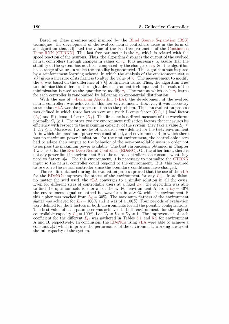
180 5. Collective Controller
Based on these premises and inspired by the Blind Source Separation (BSS)techniques, the development of the evolved neural controllers arose in the form ofan algorithm that adjusted the value of the last free parameter of the ContinuousTime RNN (CTRNN). This last free parameter is the τi, which is related with thespeed reaction of the neurons. Thus, the algorithm displaces the output of the evolvedneural controllers through changes in values of τi. It is necessary to assure that thestability of the system has not been comprised by the changes of τi. So, the algorithmhas a range of values in which the stability is guaranteed. This algorithm was inspiredby a reinforcement learning scheme, in which the analysis of the environment statuss[k] gives a measure of its flatness to alter the value of τi. The measurement to modifythe τi was based on the difference of s[k] to its mean value. Thus, the algorithm triesto minimize this difference through a descent gradient technique and the result of theminimization is used as the quantity to modify τi. The rate at which each τi learnsfor each controller is randomized by following an exponential distribution.
With the use of τ -Learning Algorithm (τLA), the development of the evolvedneural controllers was achieved in this new environment. However, it was necessaryto test that τLA was the proper solution to the problem. Thus, an evaluation processwas defined in which three factors were analysed: i) crest factor (Cf ), ii) load factor(Lf ) and iii) demand factor (Df ). The first one is a direct measure of the waveform,normally Cf ≥ 1. The other two are environment utilization factors that measures itsefficiency with respect to the maximum capacity of the system, they take a value Lf ≤1, Df ≤ 1. Moreover, two modes of actuation were defined for the test: environmentA, in which the maximum power was constrained, and environment B, in which therewas no maximum power limitation. For the first environment, the controllable usershad to adapt their output to the behavior of the non-controllable users in order notto surpass the maximum power available. The best chromosome obtained in Chapter4 was used for the Evo-Devo Neural Controller (EDeNC). On the other hand, there isnot any power limit in environment B, so the neural controllers can consume what theyneed to flatten s[k]. For this environment, it is necessary to normalize the CTRNNinput so the neural controller could respond to the environment. But, this requiredto re-evolve the neural controller since the boundary conditions have changed.
The results obtained during the evaluation process proved that the use of the τLAfor the EDeNCs improves the status of the environment for any LC . In addition,no matter the seed used, the τLA converges to a similar solution in all the cases.Even for different sizes of controllable users at a fixed LC , the algorithm was ableto find the optimum solution for all of them. For environment A, from LC = 40%the environment signal smoothed its waveform in a 80% while in environment Bthis cipher was reached from LC = 30%. The maximum flatness of the environmentsignal was achieved for LC = 100% and it was of a 100%. Four periods of evaluationwere defined for the 3 factors in both environments for all the possible configurations.The best value of each parameter was achieved in both environments for the highestcontrollable capacity LC = 100%, i.e. Cf ≈ Lf ≈ Df ≈ 1. The improvement of eachcoefficient for the different LC was gathered in Tables 5.1 and 5.2 for environmentA and B, respectively. In conclusion, the EDeNCs using τLA were able to achieve aconstant s[k] which improves the performance of the environment, working always atthe full capacity of the system.

6Neural Grid
“I’m gonna show you, how great I am” — Muhammad Ali
Regarding to the results obtained in Chapter 5, the ensemble of neuralcontrollers was able to smooth a synthetic demand curve based onthe principal frequency components of a real aggregated consumption.The neural controllers were evolved to obtain the opposed derivative
of the input signal (aggregated consumption) and cancel the variability of thecontinuous signal at their input. After that, they were developed using the τ -LearningAlgorithm (τLA) in order to cancel collectively the environment signal (aggregatedconsumption). A heterogeneous response was obtained for the different controllerswhen the algorithm was applied. Figure 6.1(a), shows an example of the behaviorof 10 users in which the controllable demand is divided. Each of them presentsa different demand profile and a flatten aggregated consumption is achieved whenadded to the non-controllable demand. Although this environment is close to a realelectric grid, it is still far from its implementation. In this Chapter, the level ofcomplexity is increased to test the development of the evolved neural controllers inan environment with real demand and Distributed Energy Resources (DER). To thisextent, the possibilities of using this kind of coordination algorithms are analyzed inreal environments. In addition, the inclusion of DER elements gives the opportunityto assess the interaction of local generation and demand, and how the controllablecapacity would help to the DER integration inside the grid.
So far, neural controllers were able to use all the power available to cancel thevariability of the non-controllable demand. However, the necessities of the users,controllable and non-controllable, must be met. Thus, the neural controllers arerestricted to use only the power from the deferrable loads which can be displacedaround the time axis. Moreover, a new criterion to displace the power of deferrableloads is developed by adding local energy resources capabilities. The controller has totake into account this new dimension of the problem in order to smooth the aggregatedconsumption plus the maximization of the local energy resource. These two objectivesare in conflict a priori. The reason is that the maximum production of Photovoltaics(PV) electricity is located at the central hours of the daylight concurring with one ofthe daily maximum consumption periods. Thus, if the consumption of all the userswere supplied locally by PV generators, the aggregated consumption would present aform such as the one of Figure 6.1(b). In this Figure, it is represented the generatedpower gPV [k] and the aggregated consumption with or without taking into account theeffect of the PV generation, sPV [k] and s[k]. The waveform of sPV [k] in Figure 6.1(b)presents a higher variability than the current behavior of the grid, s[k]. Thus, thealgorithm needs to confront a higher variability and discontinuity of the environmentsignal, which makes difficult the smoothing of the aggregated consumption.
In this Chapter, a new approximation for the neural controllers is described inorder to meet these new restrictions. An improved algorithm is built based on theuse of the neural controllers described in Chapters 4 and 5 and the addition of theusers behavior plus the DER elements. This algorithm uses the demand profilesgenerated by the Evo-Devo Neural Controllers (EDeNCs) to smooth the aggregatedconsumption in a distributed way. The EDeNC consumption patterns are usedto schedule the deferrable loads that each user allows controlling. Moreover, the
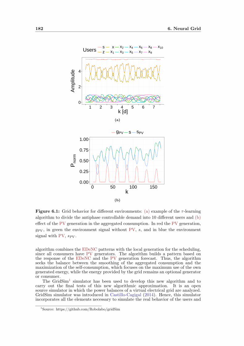
182 6. Neural Grid
0
2
4
1 2 3 4 5 6 7k [d]
Am
plitu
de
Userssz
xx1
x2
x3
x4
x5
x6
x7
x8
x9
x10
(a)
0.00
0.25
0.50
0.75
1.00
0 50 100 150k
Pno
rm
gPV s sPV
(b)
Figure 6.1: Grid behavior for different environments: (a) example of the τ -learning
algorithm to divide the antiphase controllable demand into 10 different users and (b)
effect of the PV generation in the aggregated consumption. In red the PV generation,
gPV , in green the environment signal without PV, s, and in blue the environment
signal with PV, sPV .
algorithm combines the EDeNC patterns with the local generation for the scheduling,since all consumers have PV generators. The algorithm builds a pattern based onthe response of the EDeNC and the PV generation forecast. Thus, the algorithmseeks the balance between the smoothing of the aggregated consumption and themaximization of the self-consumption, which focuses on the maximum use of the owngenerated energy, while the energy provided by the grid remains an optional generatoror consumer.
The GridSim1 simulator has been used to develop this new algorithm and tocarry out the final tests of this new algorithmic approximation. It is an opensource simulator in which the power balances of a virtual electrical grid are analyzed.GridSim simulator was introduced in Castillo-Cagigal (2014). Hence, this simulatorincorporates all the elements necessary to simulate the real behavior of the users and
1Source: https://github.com/Robolabo/gridSim
6.1. GridSim: virtual grid environment 183
Grid
Line 1
Line i
Node Node
Node Node
Node Node
Node Node
+
t
p(t)
Aggregatedconsumption
Figure 6.2: Schema of the main elements of the simulator GridSim.
the different elements of the grid into a virtual environment. A brief explanationof the simulator and its elements is included in Section 6.1. Then, the Neural GridAlgorithm (NGA) which is the new algorithm developed using the EDeNC responseis presented in Section 6.2. The scheduling of loads based on different profiles isexplained together with the control strategy followed. After that, simulations are heldto test the NGA approximation and the final tests of the EDeNC for its applicationin a virtual environment (see Section 6.3). Finally, a conclusion of the Chapter iscarried out in Section 6.4.
6.1 GridSim: virtual grid environment
GridSim is an open source software which simulates the real behavior of a grid referredto the power balance of its components. With this piece of software, simulations ofreal environments are carried out to test the NGA. The structure of the simulatorconsists of a group of nodes which are connected together through a virtual powerline. And the set of virtual power lines are connected together creating the structureof a virtual grid (see Figure 6.2). Each node is composed by different elements:
A consumption profile, whose form depends on the energy necessities of the user.Different profiles can be used in order to satisfy different users necessities. So,the profile depends on the user selected and the loads that it possesses.
A DER system consisting of a local generator with or without an storage system.In this Thesis, a PV system is used as source of the Distributed Generation(DG) and the storage system is composed by a lead-acid battery. Despite notbeing the most efficient technology, lead-acid batteries are the most known,widely used and economic technology. GridSim also offers the possibility ofincorporating other DER technologies, by changing the models used and thedifferent parameters of the element.
A controller can also be added to manage the different power flows that areconcurring inside the node by establishing different objectives to modify thenode behavior. Different controllers can be used, for example for batterymanagement or for Demand Side Management (DSM) of a set of local loads.
Thus, different types of nodes can be defined by combining the different elementsinside them. For example, there can be nodes with only consumption or generation,nodes with both of them, nodes with controllers to manage the power flows inside thevirtual grid, back-up nodes with storage systems to store electricity or any possible
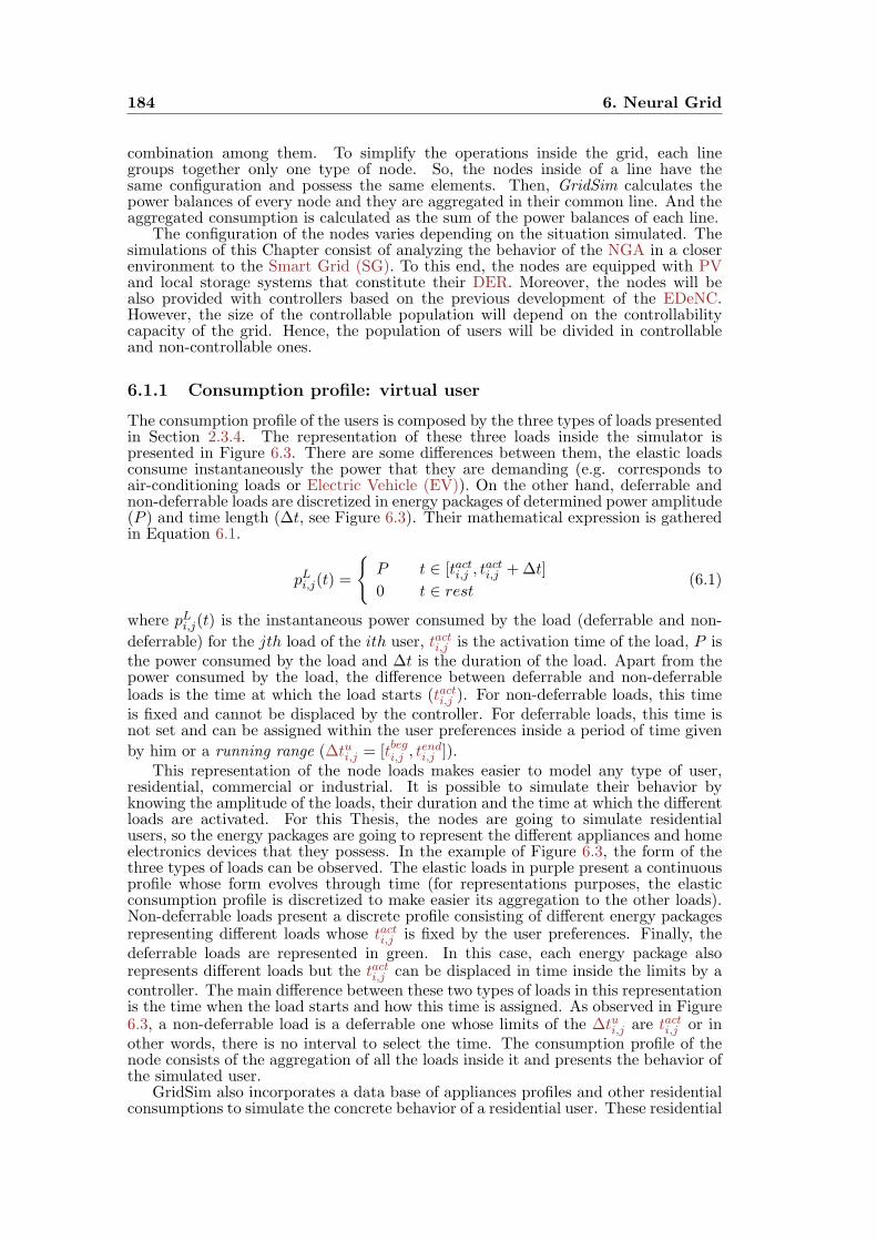
184 6. Neural Grid
combination among them. To simplify the operations inside the grid, each linegroups together only one type of node. So, the nodes inside of a line have thesame configuration and possess the same elements. Then, GridSim calculates thepower balances of every node and they are aggregated in their common line. And theaggregated consumption is calculated as the sum of the power balances of each line.
The configuration of the nodes varies depending on the situation simulated. Thesimulations of this Chapter consist of analyzing the behavior of the NGA in a closerenvironment to the Smart Grid (SG). To this end, the nodes are equipped with PVand local storage systems that constitute their DER. Moreover, the nodes will bealso provided with controllers based on the previous development of the EDeNC.However, the size of the controllable population will depend on the controllabilitycapacity of the grid. Hence, the population of users will be divided in controllableand non-controllable ones.
6.1.1 Consumption profile: virtual user
The consumption profile of the users is composed by the three types of loads presentedin Section 2.3.4. The representation of these three loads inside the simulator ispresented in Figure 6.3. There are some differences between them, the elastic loadsconsume instantaneously the power that they are demanding (e.g. corresponds toair-conditioning loads or Electric Vehicle (EV)). On the other hand, deferrable andnon-deferrable loads are discretized in energy packages of determined power amplitude(P ) and time length (∆t, see Figure 6.3). Their mathematical expression is gatheredin Equation 6.1.
pLi,j(t) =
P t ∈ [tacti,j , t
acti,j +∆t]
0 t ∈ rest(6.1)
where pLi,j(t) is the instantaneous power consumed by the load (deferrable and non-
deferrable) for the jth load of the ith user, tacti,j is the activation time of the load, P isthe power consumed by the load and ∆t is the duration of the load. Apart from thepower consumed by the load, the difference between deferrable and non-deferrableloads is the time at which the load starts (tacti,j ). For non-deferrable loads, this timeis fixed and cannot be displaced by the controller. For deferrable loads, this time isnot set and can be assigned within the user preferences inside a period of time given
by him or a running range (∆tui,j = [tbegi,j , tendi,j ]).
This representation of the node loads makes easier to model any type of user,residential, commercial or industrial. It is possible to simulate their behavior byknowing the amplitude of the loads, their duration and the time at which the differentloads are activated. For this Thesis, the nodes are going to simulate residentialusers, so the energy packages are going to represent the different appliances and homeelectronics devices that they possess. In the example of Figure 6.3, the form of thethree types of loads can be observed. The elastic loads in purple present a continuousprofile whose form evolves through time (for representations purposes, the elasticconsumption profile is discretized to make easier its aggregation to the other loads).Non-deferrable loads present a discrete profile consisting of different energy packagesrepresenting different loads whose tacti,j is fixed by the user preferences. Finally, thedeferrable loads are represented in green. In this case, each energy package alsorepresents different loads but the tacti,j can be displaced in time inside the limits by acontroller. The main difference between these two types of loads in this representationis the time when the load starts and how this time is assigned. As observed in Figure6.3, a non-deferrable load is a deferrable one whose limits of the ∆tui,j are tacti,j or inother words, there is no interval to select the time. The consumption profile of thenode consists of the aggregation of all the loads inside it and presents the behavior ofthe simulated user.
GridSim also incorporates a data base of appliances profiles and other residentialconsumptions to simulate the concrete behavior of a residential user. These residential
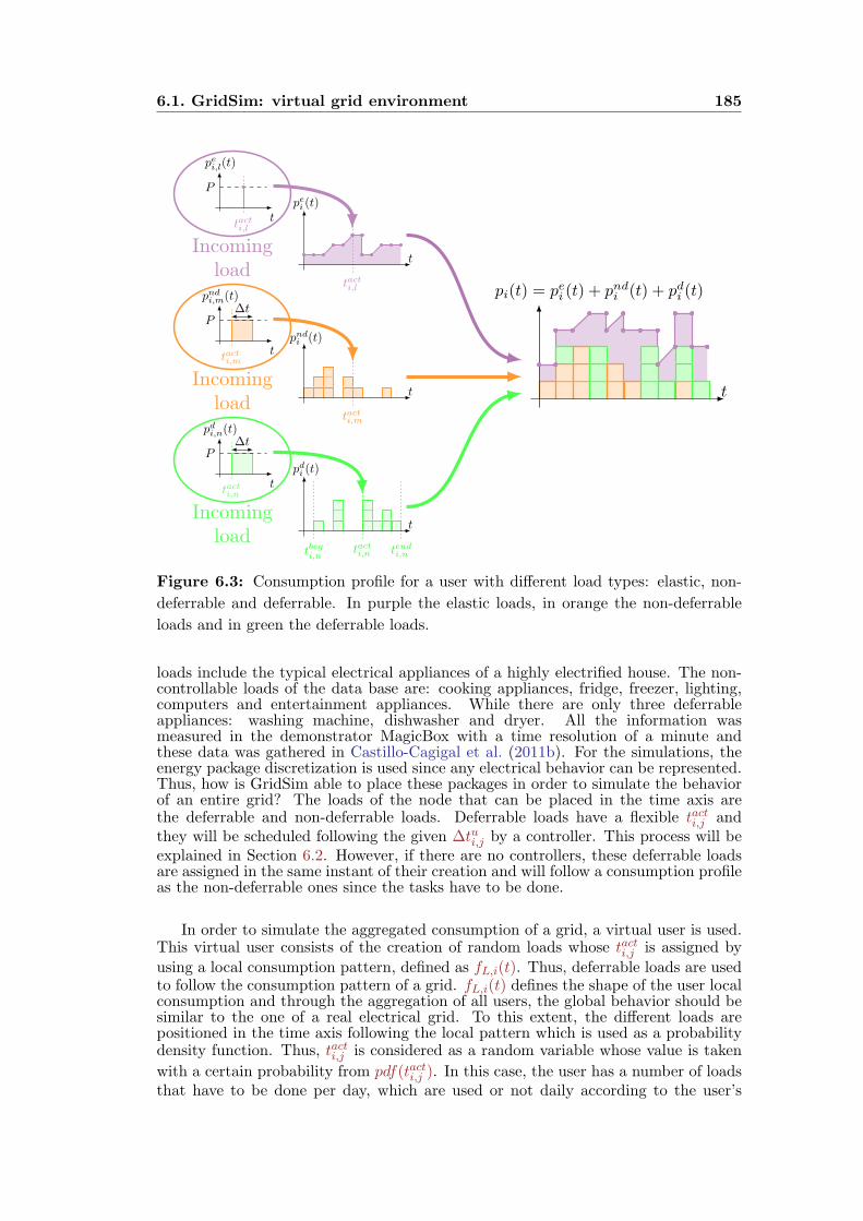
6.1. GridSim: virtual grid environment 185
P
tacti,lt
pei,l(t)
Incomingload
tacti,l
t
pei (t)
P∆t
tacti,mt
pndi,m(t)
Incomingload
tacti,m
t
pndi (t)
P∆t
tacti,nt
pdi,n(t)
Incomingload
tacti,ntbegi,n
tendi,n
t
pdi (t)
t
pi(t) = pei (t) + pndi (t) + pdi (t)
Figure 6.3: Consumption profile for a user with different load types: elastic, non-
deferrable and deferrable. In purple the elastic loads, in orange the non-deferrable
loads and in green the deferrable loads.
loads include the typical electrical appliances of a highly electrified house. The non-controllable loads of the data base are: cooking appliances, fridge, freezer, lighting,computers and entertainment appliances. While there are only three deferrableappliances: washing machine, dishwasher and dryer. All the information wasmeasured in the demonstrator MagicBox with a time resolution of a minute andthese data was gathered in Castillo-Cagigal et al. (2011b). For the simulations, theenergy package discretization is used since any electrical behavior can be represented.Thus, how is GridSim able to place these packages in order to simulate the behaviorof an entire grid? The loads of the node that can be placed in the time axis arethe deferrable and non-deferrable loads. Deferrable loads have a flexible tacti,j andthey will be scheduled following the given ∆tui,j by a controller. This process will beexplained in Section 6.2. However, if there are no controllers, these deferrable loadsare assigned in the same instant of their creation and will follow a consumption profileas the non-deferrable ones since the tasks have to be done.
In order to simulate the aggregated consumption of a grid, a virtual user is used.This virtual user consists of the creation of random loads whose tacti,j is assigned by
using a local consumption pattern, defined as fL,i(t). Thus, deferrable loads are usedto follow the consumption pattern of a grid. fL,i(t) defines the shape of the user localconsumption and through the aggregation of all users, the global behavior should besimilar to the one of a real electrical grid. To this extent, the different loads arepositioned in the time axis following the local pattern which is used as a probabilitydensity function. Thus, tacti,j is considered as a random variable whose value is taken
with a certain probability from pdf(tacti,j ). In this case, the user has a number of loadsthat have to be done per day, which are used or not daily according to the user’s
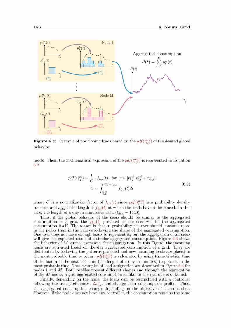
186 6. Neural Grid
Node 1
Node M
t
pdf1(t)
tact1,j
t
pL1,j(t)
tact1,j
t
pL1(t)
t
pdfM (t)
tactM,jt
pLM,j(t)
tactM,j
t
pLM (t) t
P (t)
Aggregated consumption
P (t) =M∑
i=1
pLi (t)
Figure 6.4: Example of positioning loads based on the pdf(tacti,j ) of the desired global
behavior.
needs. Then, the mathematical expression of the pdf(tacti,j ) is represented in Equation6.2.
pdf(tacti,j ) =1
C· fL,i(t) for t ∈ [tacti,j , t
acti,j + tday]
C =
∫ tacti,j +tday
tacti,j
fL,i(t)dt(6.2)
where C is a normalization factor of fL,i(t) since pdf(tacti,j ) is a probability density
function and tday is the length of fL,i(t) at which the loads have to be placed. In thiscase, the length of a day in minutes is used (tday = 1440).
Thus, if the global behavior of the users should be similar to the aggregatedconsumption of a grid, the fL,i(t) provided to the user will be the aggregatedconsumption itself. The reason is that in probability the user should consume morein the peaks than in the valleys following the shape of the aggregated consumption.One user does not have enough loads to represent it, but the aggregation of all userswill give the expected result of a similar aggregated consumption. Figure 6.4 showsthe behavior of M virtual users and their aggregation. In this Figure, the incomingloads are activated based on the day aggregated consumption of a grid. They aredistributed by following the patterns provided and new incoming loads are placed inthe most probable time to occur. pdf(tacti,j ) is calculated by using the activation time
of the load and the next 1440min (the length of a day in minutes) to place it in themost probable time. Two examples of load assignation are described in Figure 6.4 fornodes 1 and M . Both profiles present different shapes and through the aggregationof the M nodes, a grid aggregated consumption similar to the real one is obtained.
Finally, depending on the node, the loads can be rescheduled with a controllerfollowing the user preferences, ∆tui,j , and change their consumption profile. Thus,the aggregated consumption changes depending on the objective of the controller.However, if the node does not have any controller, the consumption remains the same

6.1. GridSim: virtual grid environment 187
without any change. So the virtual user will provide the local consumption of eachnode and the use of controllers will alter the grid behavior.
6.1.2 Distributed Energy Resources module
GridSim incorporates two modules related with DER: i) generation and ii) storagesystems. The different elements (consumption, generation, storage system and grid)inside a node are connected following an Alternating Current (AC) bus topologysuch as the one of Figure 4.5. The generation module inside the node is used tosimulate DG. This module only incorporates PV generation and can be configuredwith different sizes of generators. It also incorporates the elements inside a PV system,such as inverters. The generation module also takes into account the losses andefficiencies of the system through the configuration of those parameters. GridSim isable to calculate the output power of a PV system from the environment data (solarradiation and temperature), the generator parameters (size, orientation, inclination,etc.), losses factors (voltage drops, thermal, shadows, etc.) and conversion efficiencyof the inverters. So, it gives the possibility to simulate any PV generator of flat siliconPV modules.
In addition, the generation module of GridSim has an input mode in whichthe output power of a real system can be introduced to simulate different types ofgeneration. Thus, different sources of generation can be added to the simulations inorder to emulate the generation mix of real electrical grid. It is also possible to changethe PV penetration by adding more nodes. Moreover, the isolation of generationfrom the consumption is also possible through changes in the grid configuration bydefining a line with only generation and no consumption. A line can be definedper type of generation by adding nodes with no consumption plus an input file withthe power output. GridSim gives a lot of possibilities to simulate different typesof generation and their configuration in order to understand the different powerflows inside an electrical grid. In order to study the maximization of the localenergy resources, simulations are done using the PV DG systems through the useof real grid measurements. Specifically, these data correspond to the PV generationmeasurements of the Spanish peninsular system during the year 2015.
The other DER module available in GridSim that completes the node con-figuration is the storage system. The simulator allows configuring an storagesystem consisting of a battery and a bidirectional inverter that allows charging anddischarging the battery. In order to resemble to the real functioning of an storagesystem, GridSim allows configuring the conversion efficiencies of the inverter, thesize of the storage system in days of autonomy, the state of charge of the battery,the nominal voltage, etc. At the moment, only lead-acid batteries are modeledand programmed inside the simulator since their behavior are well-known and thistechnology is mature enough.
The storage system in GridSim is configured by default as a backup system whichis only discharged when the node is isolated from the grid and there is no power sourceto feed the loads. In addition, the battery is only able to charge from local energysources and never from the grid. In this way, GridSim avoids some questionabletransactions with the system, such as buying cheap electricity to sell it when it ismore expensive. By default, the battery voltage is 48V and the capacity is 1 day ofautonomy and the minimum State of Charge (SoC) is 40%. These parameters havebeen selected based on the studies of Castillo-Cagigal et al. (2011a).
All the storage system parameters can also be modified from the correspondingconfiguration file and other batteries with new materials can also be added. Moreover,the behavior of the storage system in the node can be altered by adding a controller incharge of managing the battery. Thus, the storage can be used not only as a backupsystem, but also as a local resource to supply the loads when the power of the localgenerator is not enough. Hence, in this case the grid is used as the backup system,only supplying power to the loads when there is not enough power supplied locally.In addition, the grid also receives the surplus of electricity generated that cannot beused to supply the loads or to store in the battery. Thus, the exchanges with the gridare reduced and the autonomy of the node is increased.

188 6. Neural Grid
As the generation module, the grid topology could incorporate only storagesystems that serve as backup to store the surplus of generated electricity. Therefore,the inclusion of distributed storage capacity should serve to relax the condition to meetthe demand since they can be used to adapt the electricity production to the demand.Moreover, distributed storage increases the self-consumption of local energy resources,displacing the extra generated electricity to those times where the electricity is needed.In this Chapter, the influence of these DER elements are studied from the perspectiveof the grid global behavior. To that extent, different simulations environments areconfigured.
6.2 Neural grid: scheduling with ANN and PV genera-
tion
The node configuration allows the addition of a controller to manage the differentpower flows circulating inside it. Based on the EDeNC approximation explained inChapters 4 and 5, a new algorithm is designed to manage the node power flowsand it is called Neural Grid Algorithm (NGA). The NGA is going to reschedulethe deferrable loads of the local facility in order to achieve multiple objectives: i)smoothing the aggregated consumption and ii) maximizing the use of local energyresources or maximizing the self-consumption. Thus, NGA looks for reducing theglobal variability of the grid at the same time that maximizes the self-consumption ofthe local energy sources. The facility is composed by the GridSim elements alreadypresented, a discretized consumption in energy packages and the DER.
In order to schedule the different loads, NGA will assign tacti,j of each deferrableload within ∆tui,j selected by the user. So, when a new deferrable load is created, NGA
is fed with the user preferences and it will define tacti,j based on the time preferences,assuring that time restrictions are satisfied. The algorithm uses a local consumptionpattern in order to assign tacti,j (fL,i(t), see Section 6.1.1). At the same time, fL,i(t)can be composed by different shapes which identify different objectives to schedulethe loads. Hence, NGA uses fL,i(t) as the objective form that the local consumptionshould resemble and it is also used as pdf(tacti,j ) to schedule the loads. As in Section
6.1.1, tacti,j is considered as a random variable which takes a value inside ∆tui,j with
a certain probability given by pdf(tacti,j ). In this case, the pdf(tacti,j ) form introducing∆tui,j in its definition and the temporal limits of Equation 6.2 are changed. This newform is gathered in Equation 6.3.
pdf(tacti,j ) =1
CfL,i(t
acti,j ) for tacti,j ∈ [tbegi,j , t
endi,j ]
C =
∫ tendi,j
tbegi,j
fL,i(t)dt(6.3)
where C is the normalization constant which guarantees that pdf(tacti,j ) is a probabilitydensity function. Thus, NGA will be placing the deferrable loads following the desiredlocal consumption pattern.
NGA provides the deferrable loads with the local pattern based on the twoobjectives previously stated: flattening the aggregated consumption and maximizingthe self-consumption. Thus, the fL,i(t) is also divided in two parts. The firstone corresponds to the first objective and its shape is the output of the EDeNCs,fEDeNCL,i (t). The EDeNCs have already proven that can cancel collectively thevariability of a signal. While the second one is associated with the local generationand it will have the form of the PV generation forecast, fPV
L,i (t). Therefore, fL,i(t)has the expression
fL,i(t, β) = β · fPVL,i (t) + (1− β) · fEDeNC
L,i (t) (6.4)
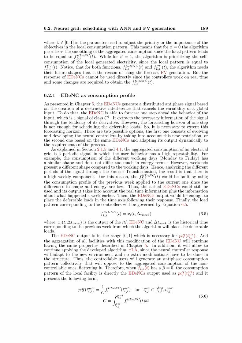
6.2. Neural grid: scheduling with ANN and PV generation 189
where β ∈ [0, 1] is the parameter used to adjust the priority or the importance of theobjectives in the local consumption pattern. This means that for β = 0 the algorithmprioritizes the smoothing of the aggregated consumption since the local pattern tendsto be equal to fEDeNC
L,i (t). While for β = 1, the algorithm is prioritizing the self-consumption of the local generated electricity, since the local pattern is equal tofPVL,i (t). Notice, that for both functions, fEDeNC
L,i (t) and fPVL,i (t), the algorithm needs
their future shapes that is the reason of using the forecast PV generation. But theresponse of EDeNCs cannot be used directly since the controllers work on real timeand some changes are required to obtain the fEDeNC
L,i (t).
6.2.1 EDeNC as consumption profile
As presented in Chapter 5, the EDeNCs generate a distributed antiphase signal basedon the creation of a destructive interference that cancels the variability of a globalinput. To do that, the EDeNC is able to forecast one step ahead the behavior of theinput, which is a signal of class C1. It extracts the necessary information of the signalthrough the tendency of its derivative. However, the forecasting horizon of one stepis not enough for scheduling the deferrable loads. So, it is necessary to extent thisforecasting horizon. There are two possible options, the first one consists of evolvingand developing the neural controllers by taking into account this new restriction, orthe second one based on the same EDeNCs and adapting its output dynamically tothe requirements of the process.
As explained in Section 2.1.5 and 4.1, the aggregated consumption of an electricalgrid is a periodic signal in which the user behavior has a high repeatability. Forexample, the consumption of the different working days (Monday to Friday) hasa similar shape and does not differ too much in energy terms. However, weekendspresent a different shape compared to the working days. Hence, analyzing the differentperiods of the signal through the Fourier Transformation, the result is that there isa high weekly component. For this reason, the fEDeNC
L,i (t) could be built by usingthe consumption profile of the previous week applied to the current one since thedifferences in shape and energy are low. Thus, the actual EDeNCs could still beused and its output takes into account the real time information plus the informationabout what happened a week earlier. Then, the EDeNCs output would be enough toplace the deferrable loads in the time axis following their response. Finally, the loadpattern corresponding to the controllers will be governed by Equation 6.5.
fEDeNCL,i (t) = xi(t,∆tweek) (6.5)
where, xi(t,∆tweek) is the output of the ith EDeNC and ∆tweek is the historical timecorresponding to the previous week from which the algorithm will place the deferrableloads.
The EDeNC output is in the range [0, 1] which is necessary for pdf(tacti,j ). Andthe aggregation of all facilities with this modification of the EDeNC will continuehaving the same properties described in Chapter 5. In addition, it will allow tocontinue applying the developed algorithm, τLA, since the neural controller responsewill adapt to the new environment and no extra modifications have to be done inthe structure. Thus, the controllable users will generate an antiphase consumptionpattern collectively that will oppose to the aggregated consumption of the non-controllable ones, flattening it. Therefore, when fL,i(t) has a β = 0, the consumptionpattern of the local facility is directly the EDeNCs output used as pdf(tacti,j ) and itpresents the following form,
pdf(tacti,j ) =1
CfEDeNCi (tacti,j ) for tacti,j ∈ [tbegi,j , t
endi,j ]
C =
∫ tendi,j
tbegi,j
fEDeNCi (t)dt
(6.6)
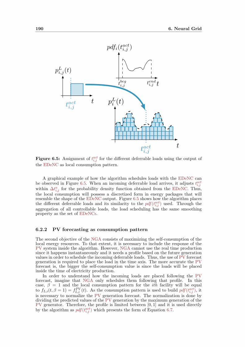
190 6. Neural Grid
tacti,jt
pLi,j(t)
tbegi,j
tendi,j t
pdfi(tacti,j )
tacti,jt
pLi (t)
Figure 6.5: Assignment of tacti,j for the different deferrable loads using the output of
the EDeNC as local consumption pattern.
A graphical example of how the algorithm schedules loads with the EDeNC canbe observed in Figure 6.5. When an incoming deferrable load arrives, it adjusts tacti,j
within ∆tui,j for the probability density function obtained from the EDeNC. Thus,the local consumption will possess a discretized form in energy packages that willresemble the shape of the EDeNC output. Figure 6.5 shows how the algorithm placesthe different deferrable loads and its similarity to the pdf(tacti,j ) used. Through theaggregation of all controllable loads, the load scheduling has the same smoothingproperty as the set of EDeNCs.
6.2.2 PV forecasting as consumption pattern
The second objective of the NGA consists of maximizing the self-consumption of thelocal energy resources. To that extent, it is necessary to include the response of thePV system inside the algorithm. However, NGA cannot use the real time productionsince it happens instantaneously and it needs a profile based on the future generationvalues in order to schedule the incoming deferrable loads. Thus, the use of PV forecastgeneration is required to place the load in the time axis. The more accurate the PVforecast is, the bigger the self-consumption value is since the loads will be placedinside the time of electricity production.
In order to understand how the incoming loads are placed following the PVforecast, imagine that NGA only schedules them following that profile. In thiscase, β = 1 and the local consumption pattern for the ith facility will be equalto fL,i(t, β = 1) = fPV
L,i (t). As the consumption pattern is used to build pdf(tacti,j ), itis necessary to normalize the PV generation forecast. The normalization is done bydividing the predicted values of the PV generation by the maximum generation of thePV generator. Therefore, the profile is limited between [0, 1] and it is used directlyby the algorithm as pdf(tacti,j ) which presents the form of Equation 6.7.
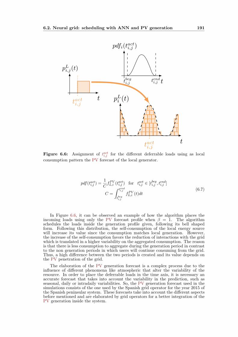
6.2. Neural grid: scheduling with ANN and PV generation 191
tacti,jt
pLi,j(t)
tbegi,j
tendi,j t
pdfi(tacti,j )
tacti,jt
pLi (t)
Figure 6.6: Assignment of tacti,j for the different deferrable loads using as local
consumption pattern the PV forecast of the local generator.
pdf(tacti,j ) =1
CfPVL,i (t
acti,j ) for tacti,j ∈ [tbegi,j , t
endi,j ]
C =
∫ tendi,j
tbegi,j
fPVL,i (t)dt
(6.7)
In Figure 6.6, it can be observed an example of how the algorithm places theincoming loads using only the PV forecast profile when β = 1. The algorithmschedules the loads inside the generation profile given, following its bell shapedform. Following this distribution, the self-consumption of the local energy sourcewill increase its value since the consumption matches local generation. However,the increase of the self-consumption favors the reduction of interactions with the gridwhich is translated in a higher variability on the aggregated consumption. The reasonis that there is less consumption to aggregate during the generation period in contrastto the non generation periods in which users will continue consuming from the grid.Thus, a high difference between the two periods is created and its value depends onthe PV penetration of the grid.
The elaboration of the PV generation forecast is a complex process due to theinfluence of different phenomena like atmospheric that alter the variability of theresource. In order to place the deferrable loads in the time axis, it is necessary anaccurate forecast that takes into account the variability in the prediction, such asseasonal, daily or intradaily variabilities. So, the PV generation forecast used in thesimulations consists of the one used by the Spanish grid operator for the year 2015 ofthe Spanish peninsular system. These forecasts take into account the different aspectsbefore mentioned and are elaborated by grid operators for a better integration of thePV generation inside the system.
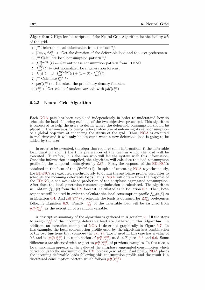
192 6. Neural Grid
Algorithm 2 High-level description of the Neural Grid Algorithm for the facility ith
of the grid.
1: /* Deferrable load information from the user */
2: [∆ti,j ,∆tui,j ]← Get the duration of the deferrable load and the user preferences
3: /* Calculate local consumption pattern */
4: fEDeNCL,i (t)← Get antiphase consumption pattern from EDeNC
5: fPVL,i (t)← Get normalized local generation forecast
6: fL,i(t) = β · fEDeNCL,i (t) + (1− β) · fPV
L,i (t)
7: /* Calculate tacti,j */
8: pdf(tacti,j )← Calculate the probability density function
9: tacti,j ← Get value of random variable with pdf(tacti,j )
6.2.3 Neural Grid Algorithm
Each NGA part has been explained independently in order to understand how toschedule the loads following each one of the two objectives presented. This algorithmis conceived to help the users to decide where the deferrable consumption should beplaced in the time axis following: a local objective of enhancing its self-consumptionor a global objective of enhancing the status of the grid. Thus, NGA is executedin real-time and it will only be activated when a new deferrable load is going to beadded by the user.
In order to be executed, the algorithm requires some information: i) the deferrableload duration and ii) the time preferences of the user in which the load will beexecuted. Therefore, it is the user who will fed the system with this information.Once the information is supplied, the algorithm will calculate the load consumptionprofile for the temporal limits given by ∆tui,j . First, the response of the EDeNC is
obtained in the form of the fEDeNCL,i (t). In spite of executing NGA asynchronously,
the EDeNCs are executed synchronously to obtain the antiphase profile, used after toschedule the incoming deferrable loads. Thus, NGA will obtain from the response ofthe EDeNC, a one week ahead prediction of the antiphase aggregated consumption.After that, the local generation resources optimization is calculated. The algorithmwill obtain fPV
L,i (t) from the PV forecast, calculated as in Equation 6.7. Then, both
responses will be used in order to calculate the local consumption profile fL,i(t, β) asin Equation 6.4. And pdf(tacti,j ) to schedule the loads is obtained for ∆tui,j preferences
following Equation 6.3. Finally, tacti,j of the deferrable load will be assigned from
pdf(tacti,j ) as the execution of a random variable.
A descriptive summary of the algorithm is gathered in Algorithm 2. All the stepsto assign tacti,j of the incoming deferrable load are gathered in this Algorithm. Inaddition, an execution example of NGA is described graphically in Figure 6.7. Inthis example, the local consumption profile used by the algorithm is a combinationof the two functions that compose the fL,i(t). The β used in this case has a value of0.5 and its pdf(tacti,j ) is a combination of pdf(tacti,j ) used in Figures 6.5 and 6.6. Some
differences are observed with respect to pdf(tacti,j ) of previous examples. In this case, alocal maximum appears at the valley of the antiphase aggregated consumption whichcorresponds to the maximum of the PV forecast generation. And finally, NGA placesthe incoming deferrable loads following this consumption profile and the result is adiscretized consumption pattern which follows pdf(tacti,j ).

6.3. Simulation Results 193
tacti,jt
pLi,j(t)
tbegi,j
tendi,j t
pdfi(tacti,j )
tacti,jt
pLi (t)
Figure 6.7: Assignment of tacti,j based on the combined consumption profiles selected
by the algorithm.
6.3 Simulation Results
After enunciating the proposed NGA, it is necessary to test the hypothesis suggested.The algorithm is analyzed in a simulation environment carried out in GridSim (seeSection 6.1). The evaluation process consists of a series of simulated experiments inwhich the benefits of using NGA in an electrical grid are tested. To that extent, eachexperiment analyzes different parts of the algorithm in different environments whereit could improve the grid status. The simulations were divided into three differentphases:
Analysis of the EDeNC response. In this set of simulations, the part of theNGA corresponding to the flattening of the aggregated consumption is analyzed.Thus, each facility will be composed only by loads and there will be no localenergy resource available to feed them. In order to test the response of the NGA,the controllable fraction LC of the facilities will be varied. However, the EDeNCresponse has not been tested in a real environment. Thus, a first experimentwill consist of using directly the EDeNC over elastic loads and varying the LCin order to smooth the aggregated consumption (see Section 6.3.3). Once thecontrollers have been tested, in the next experiment NGA will schedule thedeferrable loads only by using the delayed consumption profiles given by theEDeNC, so β = 0 (see Section 6.3.4).
Analysis of the NGA with DG. In this case, PV generation is added locally toall facilities without an storage system. This set of experiments will evaluatethe NGA capacity to meet the two proposed objectives, the smoothing of theaggregated consumption and the maximization of the local energy sources.To this end, LC and PVp will vary and NGA will search for the equilibriumbetween both objectives by scheduling the deferrable loads properly. In a firstexperiment, NGA will integrate PV generation by only scheduling loads by
194 6. Neural Grid
following the smoothing of aggregated consumption (see Section 6.3.5). Afteranalyzing the variability that PV introduces, NGA will schedule loads for theworst scenario following the two objectives by varying the value of β (see Section6.3.6).
Analysis of the NGA with DER. Finally, in the last simulations, the environmentwill also incorporate an storage system together with local PV electricitygenerator. The storage system is only able to charge the battery from thelocal surplus of generated electricity. Thus, it can be possible to defer theconsumption of previously generated energy over time. In this experiment,NGA schedules the deferrable loads trying to reduce the variability of the gridand consuming as much as possible from the local sources. Those effects areanalyzed varying the PVp and the storage capacity (see Section 6.3.7)
In order to perform this analysis, the environment has been set following theelements configuration of Section 6.3.1, and all the different figures of merit used inthe analysis are described in Section 6.3.2.
6.3.1 Environment configuration
For all the simulations, the aggregated consumption profile used corresponds to theone of the Spanish peninsular grid during 2015 according to official data providedby the grid operator Red Electrica de Espana (REE)2. The grid is divided in nodeswhose local consumption is created by the virtual user already described in Section6.1.1. Although the simulator allows creating as many nodes per lines as possible,the computation resources have limited the number of nodes that can be simulated.Thus, the number of nodes in which the grid is divided has been limited to 600 whichare enough to study the behavior of the NGA.
Each node is composed by a virtual user in charge of the consumption, a PVgenerator and an storage system. The last two elements would be included in thesimulations depending on the requirements of the experiment. In this case, theenvironment has been escalated to the mentioned number of nodes and each noderepresents more than one facility. So each node consists of the aggregation of variousfacilities composed by the same elements (consumption, PV generation and storagesystem).
The virtual user is in charge of creating the different loads of the node. All theloads created by the virtual user are deferrable and their tacti,j is assigned following thelocal consumption pattern. In addition, this user will create the loads randomly andthey can be created at any time during the simulation. If they are not scheduled byany controller, they will be executed at the creation time of the virtual user. For thesimulations the length of the time step used is of 1min. In the absence of a controller,each virtual user is going to follow the aggregated consumption pattern provided.
Nevertheless, each virtual user has a number of deferrable loads that can be createdper period of time to simulate the same amount of energy that a local facility canconsume. The virtual user has a window of time to set its deferrable loads of 1 dayor 1440min. Each deferrable load consists of an energy packet of a power amplitudeof P = 50MW and a duration of ∆t = 60min. So, for the simulated grid to beequal to the real one, it is necessary that the energy consumed in both of them isthe same. The Spanish grid in 2015 has a total energy consumption of 248TWh, sothe energy consumed per node in the simulator will be equal to 414GWh. Finally,a node possesses around 8300 deferrable loads per year to simulate the behavior ofthe Spanish grid based on the energy consumed per node and the amplitude of theenergy packets.
With respect to the local PV generation, the data used corresponds to the totalpredicted and measured PV generation of the Spanish grid for the year 20153. Theshape of the generation is extracted directly from this data. In order to incorporate
2Spanish peninsular grid measurements, source: R.E.E. e-sios3PV generation forecasts and measurements, source: R.E.E. e-sios
6.3. Simulation Results 195
inside the simulation, the data is normalized by the maximum generation of the year.The reason is that the amount of generated power varies in order to analyze the effectof different percentages of PVp. For a PVp= 100%, the maximum nominal power ofthe generator is 240MWp per node, such that the sum of the generation of all nodesis 144GWp. This maximum nominal power is selected for the generator to producethe same amount of energy consumed in Spain in 2015, i.e. around 248TWh.
The last element included in the simulations is an storage system per node. Thissimulated system consists of a battery inverter, a lead-acid battery and a batterycontroller. The capacity of the battery is modified in order to study its effects inthe variability of the grid. Thus, the capacity of the battery is varied from theabsence of capacity to 2 days of autonomy. The inverter parameters are adjusted tothe battery and the controller will only charge the battery with the surplus of PVelectricity. Hence, the function of the battery controller is double, maximizing theself-consumption without compromising the battery lifetime avoiding its over-chargeand over-discharge situations.
6.3.2 Evaluation process
Each experiment is executed during 13months or 568800min. The first month is usedby the algorithm to stabilize and the evaluation is done during the remaining time.NGA has been built by following two objectives. Thus, different figures of merit areneeded to evaluate each part of the algorithm. In order to evaluate the smoothnessof the aggregated consumption, the method selected analyzes its waveform. Whereasfor the analysis of the second objective, a figure that relates the energy consumedwith the one produced is required. In particular:
Analysis of the aggregated consumption variability. It has been conductedprimarily with the crest factor figure of merit (Cf ), already used previously (seeSections 4.4 and 5.3). The mathematical expression is contained in Equation4.31 and as a reminder, Cf is a relationship of the maximum of a signal withrespect to its effective value during a period of time.For those experiments in which there is no local generation, the load factor (Lf )and demand factor (Df ) are also used as in the evaluation process of Section5.3. The mathematical expression of the Lf is included in Equation 5.25 andfor Df is in Equation 5.26. Both of them are figures of merit used not onlyto analyze the form of the aggregated consumption but also the use that thedifferent nodes of the grid made of the resource. In all the cases, the best valueis 1 and they are evaluated for different periods of time, specifically: i) daily, ii)weekly, iii) monthly and iv) annually. The 3 evaluation parameters are averagedfor this 4 periods of time as in Equation 5.27.
Analysis of the self-consumption. In order to evaluate the second part of theNGA, it is necessary to define a new figure of merit. This figure should assessthe amount of energy from the local energy resources that feed the consumption.Thus, the self-consumption factor (ξ) is defined as the fraction of the electricalenergy consumed by the loads which is only supplied by the local generationsources (Castillo-Cagigal et al., 2011b,a). The self-consumption factor has twovariants depending on the term used to normalize it:
– Consumption normalization. It is defined as the fraction of load that issupplied (directly and indirectly) from the PV system. The mathematicalexpression is collected in Equation 6.8.
ξL =EDER
EL=
EPV,L + EBat,L
EL(6.8)
where EL is the total energy consumed by the loads and EDER is theelectrical energy generated locally which in this case is divided in: EPV,L,the energy directly supplied by the PV generator to the loads, and EBat,L,

196 6. Neural Grid
the PV origin energy supplied by the storage system to the loads. Noticethat depending on the environment configuration, the term EBat,L couldbe zero and it represents the deferred use of the PV generated electricityin time.
– Generation normalization. It is defined as the fraction of generatedelectricity that is used to supply the loads and it is defined as
ξG =EDER
EG=
EPV,L + EBat,L
EG(6.9)
where EG is the total generated electricity locally by the PV system.
ξL expresses the independence of the user over the grid while ξG representsthe use of the local generated electricity to meet the demand of a user. Sincethe direct and indirect local use of PV production ultimately depends on thedemand, it can be concluded that ξL ∈ [0, 1] and ξG ∈ [0, 1]. However, themeaning of each factor is different. A ξL = 0 means that the node has noavailable local generation, while a value of ξL = 1 means that the energyconsumed by the node is totally supplied by the local energy generation sources.On the other hand, ξG = 0 means that all the generated electricity goes to thegrid and the user does not self-consume anything, and a ξG = 1 means thatall the generated electricity supplies the local demand. It should be notedthat both proposed factors could be used in different time frames. In addition,because they are normalized, comparisons between the ξ of PV systems withdifferent sizes and loads are possible. However, only the ξL is used as theassessment factor for the simulations with local DER. The reason is that duringthe simulations, the energy consumed by the nodes is fixed and the DER sizesare varied in order to quantify their effects over the consumption.
6.3.3 Direct load control
In this first experiment, the EDeNC response is going to be tested in a realenvironment. The environment is composed only by consumption nodes, there isno local generation. Each node is equipped with a virtual user and the numberof controllers varies depending on the LC , the fraction of total consumption that iscontrollable. The consumption is composed by two different types of loads: deferrable,to create an aggregated consumption similar to one given, and elastic, to evaluate thecontrollable capabilities of the users.
Virtual users create deferrable loads following the local consumption pattern ofthe Spanish grid, but the EDeNCs are not scheduling tacti,j of the loads. Thus, thedeferrable loads are going to be executed when they are created. On the other hand,those nodes equipped with an EDeNC will use elastic loads in order to smooth theaggregated consumption. The EDeNCs modify directly the consumed power of theelastic loads. Thus, the power that these loads consume is given by multiplying thenormalized output of the EDeNC by the maximum power that they can consume. Inaddition, the response of the controllers is executed in real time without taking intoaccount the one week history information to elaborate it.
During the experiment, LC is the percentage of nodes that is controllable. Eachsimulation used a different percentage of LC and varies from 0% to 100%. As thedeferrable loads of the virtual users are assigned randomly, each simulation is repeatedfor 30 different seeds per percentage of LC . With this number of seeds, the dispersionfor each realization is observed in order to validate statistically the experiment. Theresults of this experiment are represented in Figure 6.8.
Each panel of Figure 6.8 represents the median of each parameter for each of the30 seeds used to evaluate each percentage of LC . The deviation per simulation isalso represented in shadow grey, but the 1st and the 3rd quartile are too close to themedian so it is negligible. Thus, the EDeNCs achieve a very similar solution for all theseeds. In general, from the results of Figure 6.8, it can be observed that the tendency

6.3. Simulation Results 197
Day Week
Month Year
0.8
1.0
1.2
1.4
0.8
1.0
1.2
1.4
0 20 40 60 80 100 0 20 40 60 80 100
LC [%]
Am
plitu
deFigures Cf Df Lf
Figure 6.8: Evaluation of the EDeNC to control directly the power of elastic loads
in real time. In black Cf per period of time, in blue Df per period of time and in red
Lf per period of time.
for all the three parameters in all periods of evaluation tends to the best value of eachof them, 1, thus achieving the desired outcome (aggregated curve smoothed).
The first parameter to analyze is the Cf . For no controllable capacity in the
environment, the median Cf obtained per period are: 1.16 daily, 1.24 weekly, 1.29
monthly and 1.43 annually. With respect to the trend of the Cf value, it decreasesas the LC grows, but it can be observed in Figure 6.8 that there is a change of slopefor LC = 30%. Cf decreases rapidly for LC values less than this point and thendecays slowly for bigger values of LC until it reaches its minimum at LC = 100%. Ata LC = 30%, the Cf value per period has decreased in 12.59% daily, 19.13% weekly,22.50% monthly and 30.58% annually with respect to the absence of controllabilitycapacity, LC = 0%. Finally, Cf reaches its minimum at the end of the experiment for
LC = 100%. Thus, the Cf suffers a decrease in percentage of 16.50% daily, 24.87%weekly, 29.66% monthly and 42.71% annually comparing the starting LC = 0% andending LC = 100%. Thus, the inclusion of controllable elements in the environmentenhances the grid status since its variability is reduced. Table 6.1 shows the resultsfor all controllable capacities
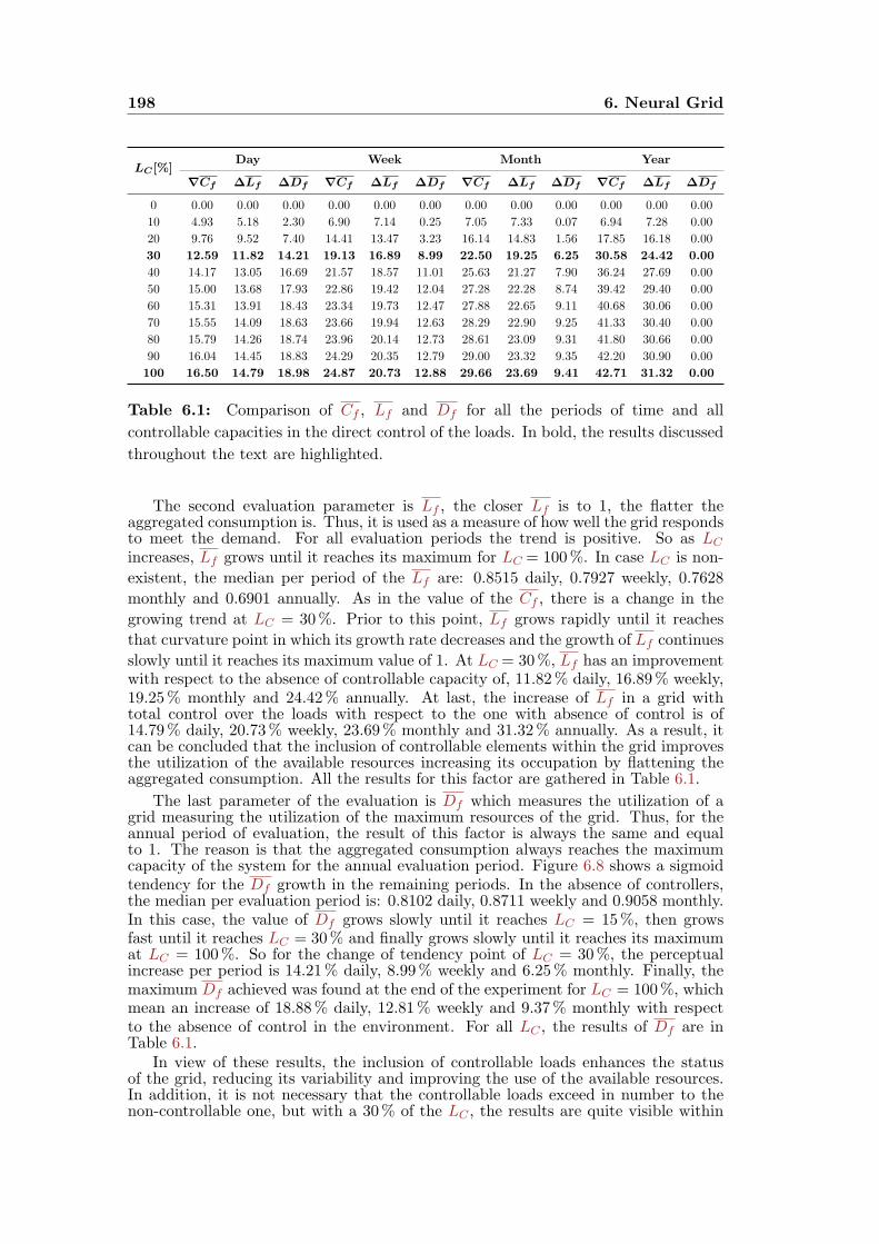
198 6. Neural Grid
LC[%]Day Week Month Year
∇Cf ∆Lf ∆Df ∇Cf ∆Lf ∆Df ∇Cf ∆Lf ∆Df ∇Cf ∆Lf ∆Df
0 0.00 0.00 0.00 0.00 0.00 0.00 0.00 0.00 0.00 0.00 0.00 0.00
10 4.93 5.18 2.30 6.90 7.14 0.25 7.05 7.33 0.07 6.94 7.28 0.00
20 9.76 9.52 7.40 14.41 13.47 3.23 16.14 14.83 1.56 17.85 16.18 0.00
30 12.59 11.82 14.21 19.13 16.89 8.99 22.50 19.25 6.25 30.58 24.42 0.00
40 14.17 13.05 16.69 21.57 18.57 11.01 25.63 21.27 7.90 36.24 27.69 0.00
50 15.00 13.68 17.93 22.86 19.42 12.04 27.28 22.28 8.74 39.42 29.40 0.00
60 15.31 13.91 18.43 23.34 19.73 12.47 27.88 22.65 9.11 40.68 30.06 0.00
70 15.55 14.09 18.63 23.66 19.94 12.63 28.29 22.90 9.25 41.33 30.40 0.00
80 15.79 14.26 18.74 23.96 20.14 12.73 28.61 23.09 9.31 41.80 30.66 0.00
90 16.04 14.45 18.83 24.29 20.35 12.79 29.00 23.32 9.35 42.20 30.90 0.00
100 16.50 14.79 18.98 24.87 20.73 12.88 29.66 23.69 9.41 42.71 31.32 0.00
Table 6.1: Comparison of Cf , Lf and Df for all the periods of time and all
controllable capacities in the direct control of the loads. In bold, the results discussed
throughout the text are highlighted.
The second evaluation parameter is Lf , the closer Lf is to 1, the flatter theaggregated consumption is. Thus, it is used as a measure of how well the grid respondsto meet the demand. For all evaluation periods the trend is positive. So as LC
increases, Lf grows until it reaches its maximum for LC = 100%. In case LC is non-
existent, the median per period of the Lf are: 0.8515 daily, 0.7927 weekly, 0.7628
monthly and 0.6901 annually. As in the value of the Cf , there is a change in the
growing trend at LC = 30%. Prior to this point, Lf grows rapidly until it reaches
that curvature point in which its growth rate decreases and the growth of Lf continues
slowly until it reaches its maximum value of 1. At LC = 30%, Lf has an improvementwith respect to the absence of controllable capacity of, 11.82% daily, 16.89% weekly,19.25% monthly and 24.42% annually. At last, the increase of Lf in a grid withtotal control over the loads with respect to the one with absence of control is of14.79% daily, 20.73% weekly, 23.69% monthly and 31.32% annually. As a result, itcan be concluded that the inclusion of controllable elements within the grid improvesthe utilization of the available resources increasing its occupation by flattening theaggregated consumption. All the results for this factor are gathered in Table 6.1.
The last parameter of the evaluation is Df which measures the utilization of agrid measuring the utilization of the maximum resources of the grid. Thus, for theannual period of evaluation, the result of this factor is always the same and equalto 1. The reason is that the aggregated consumption always reaches the maximumcapacity of the system for the annual evaluation period. Figure 6.8 shows a sigmoidtendency for the Df growth in the remaining periods. In the absence of controllers,the median per evaluation period is: 0.8102 daily, 0.8711 weekly and 0.9058 monthly.In this case, the value of Df grows slowly until it reaches LC = 15%, then growsfast until it reaches LC = 30% and finally grows slowly until it reaches its maximumat LC = 100%. So for the change of tendency point of LC = 30%, the perceptualincrease per period is 14.21% daily, 8.99% weekly and 6.25% monthly. Finally, themaximum Df achieved was found at the end of the experiment for LC = 100%, whichmean an increase of 18.88% daily, 12.81% weekly and 9.37% monthly with respectto the absence of control in the environment. For all LC , the results of Df are inTable 6.1.
In view of these results, the inclusion of controllable loads enhances the statusof the grid, reducing its variability and improving the use of the available resources.In addition, it is not necessary that the controllable loads exceed in number to thenon-controllable one, but with a 30% of the LC , the results are quite visible within

6.3. Simulation Results 199
the grid. However, in this experiment the EDeNCs have total access to the powerof the loads because they are elastic ones. So, it is necessary to move a step closerto the reality since the loads that allow accessing them and changing directly theirpower are few.
6.3.4 Random deferrable loads
Once the EDeNC response has been tested successfully, it is necessary to use them in acloser environment to the reality. In this experiment, the smoothing of the aggregatedconsumption is tested by using the EDeNC part of the NGA. As in the experimentof Section 6.3.3, the grid is composed only by consuming nodes and there is no DERinside them. However, the type of loads that compose the node consumption consistsonly of deferrable loads. Then, each node is equipped with a virtual user and thecontrol capacity varies depending on the percentage of LC .
The virtual users inside the nodes are the ones in charge of creating the deferrableloads using as consumption pattern the Spanish aggregated consumption. Dependingon LC , NGA is going to schedule the deferrable loads created by the virtual user. Sofor those nodes without NGA, their loads are executed in their creation time. As theoutput of the EDeNC is normalized, it can be used directly for the assignment of tacti,j .The execution of the loads is in real time, but the actions to schedule them are takenone day in advance in order to assign tacti,j .
The grid is formed by 600 nodes from which an LC percentage of nodes are ableto actuate over the scheduling time of the deferrable loads through the use of NGA.During the experiment the percentage of LC is varied from 0% to 100%, i.e. fromthe absence of load control in the environment to its total control. As the loads areassigned randomly by the virtual users, each simulation was executed 30 times withdifferent seeds. So, the necessity of using various seeds consists of evaluating therepeatability and dispersion of the solutions found by the algorithm for different loadcollocations in the times axis. This number of seeds is enough to validate statisticallythe experiment. Figure 6.9 shows the results of this experiment.
Each panel of Figure 6.9 represents a period of evaluation, from daily to annually.In each panel, the median of the average performance of each coefficient is representedin the period of evaluation for the 30 seeds in which each simulation is composed.Moreover, the deviation of each point of the median is represented in shadow grey.However, the distance of the 1st and the 3rd quartile with respect to the median is sosmall that it is negligible. Thus, NGA found a similar solution per each configurationof the experiment. As the previous experiment results, in Figure 6.9 can be observedthat all coefficients reach the best value at the end of the simulation and the tendenciesof each parameter are not as pronounced as in Figure 6.8.
With respect to the waveform of the aggregated consumption, the Cf isrepresented in black in Figure 6.8. In case of no control over the activation of thedeferrable loads, the value of Cf per period is of: 1.16 daily, 1.24 weekly, 1.28 monthlyand 1.41 annually. These values are very similar to the ones of Section 6.3.3. But ingeneral, for all the evaluations periods, the decreasing tendency of Cf in Figure 6.9is slower than the one of Figure 6.8. The reason is that the direct control allows tolocate the exact quantity to be in antiphase to the aggregated consumption. Thus,the discretization error of the consumption profile plus the prediction error of usingthe EDeNC response produce values above 1 for Cf . In this case, the decreasingtendency is more linear than exponential as in the previous experiment. Therefore,at the middle of the simulation (LC = 50%), the values of Cf correspond to adecrease of the 5.83% daily, the 7.35% weekly, the 9.44% monthly and the 11.90%annually with respect to the absence of controllability capacity. At last, Cf reaches
its minimum at LC = 100%. Thus, the Cf has decreased in percentage an amount of7.45% daily, 11.41% weekly, 13.37% monthly and 19.55% annually with respect tothe beginning of the experiment at LC = 0%. In spite of the results being far fromthe unity in all periods, the inclusion of controllable elements in the grid flattens the
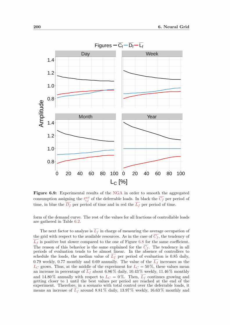
200 6. Neural Grid
Day Week
Month Year
0.8
1.0
1.2
1.4
0.8
1.0
1.2
1.4
0 20 40 60 80 100 0 20 40 60 80 100
LC [%]
Am
plitu
deFigures Cf Df Lf
Figure 6.9: Experimental results of the NGA in order to smooth the aggregated
consumption assigning the tacti,j of the deferrable loads. In black the Cf per period of
time, in blue the Df per period of time and in red the Lf per period of time.
form of the demand curve. The rest of the values for all fractions of controllable loadsare gathered in Table 6.2.
The next factor to analyze is Lf in charge of measuring the average occupation of
the grid with respect to the available resources. As in the case of Cf , the tendency of
Lf is positive but slower compared to the one of Figure 6.8 for the same coefficient.
The reason of this behavior is the same explained for the Cf . The tendency in allperiods of evaluation tends to be almost linear. In the absence of controllers toschedule the loads, the median value of Lf per period of evaluation is 0.85 daily,
0.79 weekly, 0.77 monthly and 0.69 annually. The value of the Lf increases as theLC grows. Thus, at the middle of the experiment for LC = 50%, these values meanan increase in percentage of Lf about 6.86% daily, 10.43% weekly, 11.46% monthly
and 14.80% annually with respect to LC = 0%. Then, Lf continues growing andgetting closer to 1 until the best values per period are reached at the end of theexperiment. Therefore, in a scenario with total control over the deferrable loads, itmeans an increase of Lf around 8.81% daily, 13.97% weekly, 16.63% monthly and
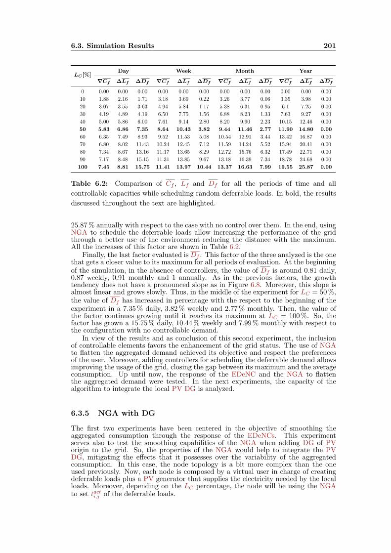
6.3. Simulation Results 201
LC[%]Day Week Month Year
∇Cf ∆Lf ∆Df ∇Cf ∆Lf ∆Df ∇Cf ∆Lf ∆Df ∇Cf ∆Lf ∆Df
0 0.00 0.00 0.00 0.00 0.00 0.00 0.00 0.00 0.00 0.00 0.00 0.00
10 1.88 2.16 1.71 3.18 3.69 0.22 3.26 3.77 0.06 3.35 3.98 0.00
20 3.07 3.55 3.63 4.94 5.84 1.17 5.38 6.31 0.95 6.1 7.25 0.00
30 4.19 4.89 4.19 6.50 7.75 1.56 6.88 8.23 1.33 7.63 9.27 0.00
40 5.00 5.86 6.00 7.61 9.14 2.80 8.20 9.90 2.23 10.15 12.46 0.00
50 5.83 6.86 7.35 8.64 10.43 3.82 9.44 11.46 2.77 11.90 14.80 0.00
60 6.35 7.49 8.93 9.52 11.53 5.08 10.54 12.91 3.44 13.42 16.87 0.00
70 6.80 8.02 11.43 10.24 12.45 7.12 11.59 14.24 5.52 15.94 20.41 0.00
80 7.34 8.67 13.16 11.17 13.65 8.29 12.72 15.76 6.32 17.49 22.71 0.00
90 7.17 8.48 15.15 11.31 13.85 9.67 13.18 16.39 7.34 18.78 24.68 0.00
100 7.45 8.81 15.75 11.41 13.97 10.44 13.37 16.63 7.99 19.55 25.87 0.00
Table 6.2: Comparison of Cf , Lf and Df for all the periods of time and all
controllable capacities while scheduling random deferrable loads. In bold, the results
discussed throughout the text are highlighted.
25.87% annually with respect to the case with no control over them. In the end, usingNGA to schedule the deferrable loads allow increasing the performance of the gridthrough a better use of the environment reducing the distance with the maximum.All the increases of this factor are shown in Table 6.2.
Finally, the last factor evaluated is Df . This factor of the three analyzed is the onethat gets a closer value to its maximum for all periods of evaluation. At the beginningof the simulation, in the absence of controllers, the value of Df is around 0.81 daily,0.87 weekly, 0.91 monthly and 1 annually. As in the previous factors, the growthtendency does not have a pronounced slope as in Figure 6.8. Moreover, this slope isalmost linear and grows slowly. Thus, in the middle of the experiment for LC = 50%,the value of Df has increased in percentage with the respect to the beginning of theexperiment in a 7.35% daily, 3.82% weekly and 2.77% monthly. Then, the value ofthe factor continues growing until it reaches its maximum at LC = 100%. So, thefactor has grown a 15.75% daily, 10.44% weekly and 7.99% monthly with respect tothe configuration with no controllable demand.
In view of the results and as conclusion of this second experiment, the inclusionof controllable elements favors the enhancement of the grid status. The use of NGAto flatten the aggregated demand achieved its objective and respect the preferencesof the user. Moreover, adding controllers for scheduling the deferrable demand allowsimproving the usage of the grid, closing the gap between its maximum and the averageconsumption. Up until now, the response of the EDeNC and the NGA to flattenthe aggregated demand were tested. In the next experiments, the capacity of thealgorithm to integrate the local PV DG is analyzed.
6.3.5 NGA with DG
The first two experiments have been centered in the objective of smoothing theaggregated consumption through the response of the EDeNCs. This experimentserves also to test the smoothing capabilities of the NGA when adding DG of PVorigin to the grid. So, the properties of the NGA would help to integrate the PVDG, mitigating the effects that it possesses over the variability of the aggregatedconsumption. In this case, the node topology is a bit more complex than the oneused previously. Now, each node is composed by a virtual user in charge of creatingdeferrable loads plus a PV generator that supplies the electricity needed by the localloads. Moreover, depending on the LC percentage, the node will be using the NGAto set tacti,j of the deferrable loads.
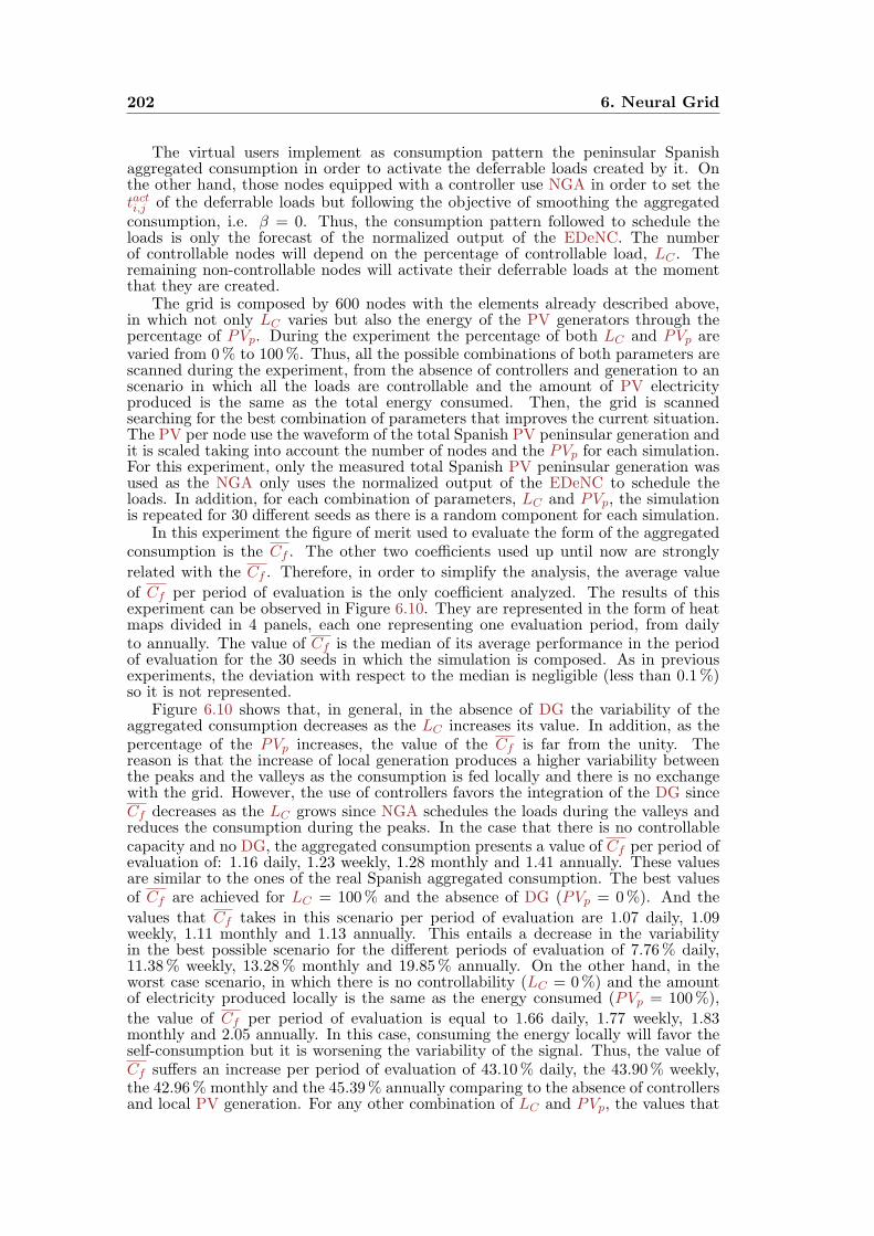
202 6. Neural Grid
The virtual users implement as consumption pattern the peninsular Spanishaggregated consumption in order to activate the deferrable loads created by it. Onthe other hand, those nodes equipped with a controller use NGA in order to set thetacti,j of the deferrable loads but following the objective of smoothing the aggregatedconsumption, i.e. β = 0. Thus, the consumption pattern followed to schedule theloads is only the forecast of the normalized output of the EDeNC. The numberof controllable nodes will depend on the percentage of controllable load, LC . Theremaining non-controllable nodes will activate their deferrable loads at the momentthat they are created.
The grid is composed by 600 nodes with the elements already described above,in which not only LC varies but also the energy of the PV generators through thepercentage of PVp. During the experiment the percentage of both LC and PVp arevaried from 0% to 100%. Thus, all the possible combinations of both parameters arescanned during the experiment, from the absence of controllers and generation to anscenario in which all the loads are controllable and the amount of PV electricityproduced is the same as the total energy consumed. Then, the grid is scannedsearching for the best combination of parameters that improves the current situation.The PV per node use the waveform of the total Spanish PV peninsular generation andit is scaled taking into account the number of nodes and the PVp for each simulation.For this experiment, only the measured total Spanish PV peninsular generation wasused as the NGA only uses the normalized output of the EDeNC to schedule theloads. In addition, for each combination of parameters, LC and PVp, the simulationis repeated for 30 different seeds as there is a random component for each simulation.
In this experiment the figure of merit used to evaluate the form of the aggregatedconsumption is the Cf . The other two coefficients used up until now are strongly
related with the Cf . Therefore, in order to simplify the analysis, the average value
of Cf per period of evaluation is the only coefficient analyzed. The results of thisexperiment can be observed in Figure 6.10. They are represented in the form of heatmaps divided in 4 panels, each one representing one evaluation period, from dailyto annually. The value of Cf is the median of its average performance in the periodof evaluation for the 30 seeds in which the simulation is composed. As in previousexperiments, the deviation with respect to the median is negligible (less than 0.1%)so it is not represented.
Figure 6.10 shows that, in general, in the absence of DG the variability of theaggregated consumption decreases as the LC increases its value. In addition, as thepercentage of the PVp increases, the value of the Cf is far from the unity. Thereason is that the increase of local generation produces a higher variability betweenthe peaks and the valleys as the consumption is fed locally and there is no exchangewith the grid. However, the use of controllers favors the integration of the DG sinceCf decreases as the LC grows since NGA schedules the loads during the valleys andreduces the consumption during the peaks. In the case that there is no controllablecapacity and no DG, the aggregated consumption presents a value of Cf per period ofevaluation of: 1.16 daily, 1.23 weekly, 1.28 monthly and 1.41 annually. These valuesare similar to the ones of the real Spanish aggregated consumption. The best valuesof Cf are achieved for LC = 100% and the absence of DG (PVp = 0%). And the
values that Cf takes in this scenario per period of evaluation are 1.07 daily, 1.09weekly, 1.11 monthly and 1.13 annually. This entails a decrease in the variabilityin the best possible scenario for the different periods of evaluation of 7.76% daily,11.38% weekly, 13.28% monthly and 19.85% annually. On the other hand, in theworst case scenario, in which there is no controllability (LC = 0%) and the amountof electricity produced locally is the same as the energy consumed (PVp = 100%),
the value of Cf per period of evaluation is equal to 1.66 daily, 1.77 weekly, 1.83monthly and 2.05 annually. In this case, consuming the energy locally will favor theself-consumption but it is worsening the variability of the signal. Thus, the value ofCf suffers an increase per period of evaluation of 43.10% daily, the 43.90% weekly,the 42.96% monthly and the 45.39% annually comparing to the absence of controllersand local PV generation. For any other combination of LC and PVp, the values that
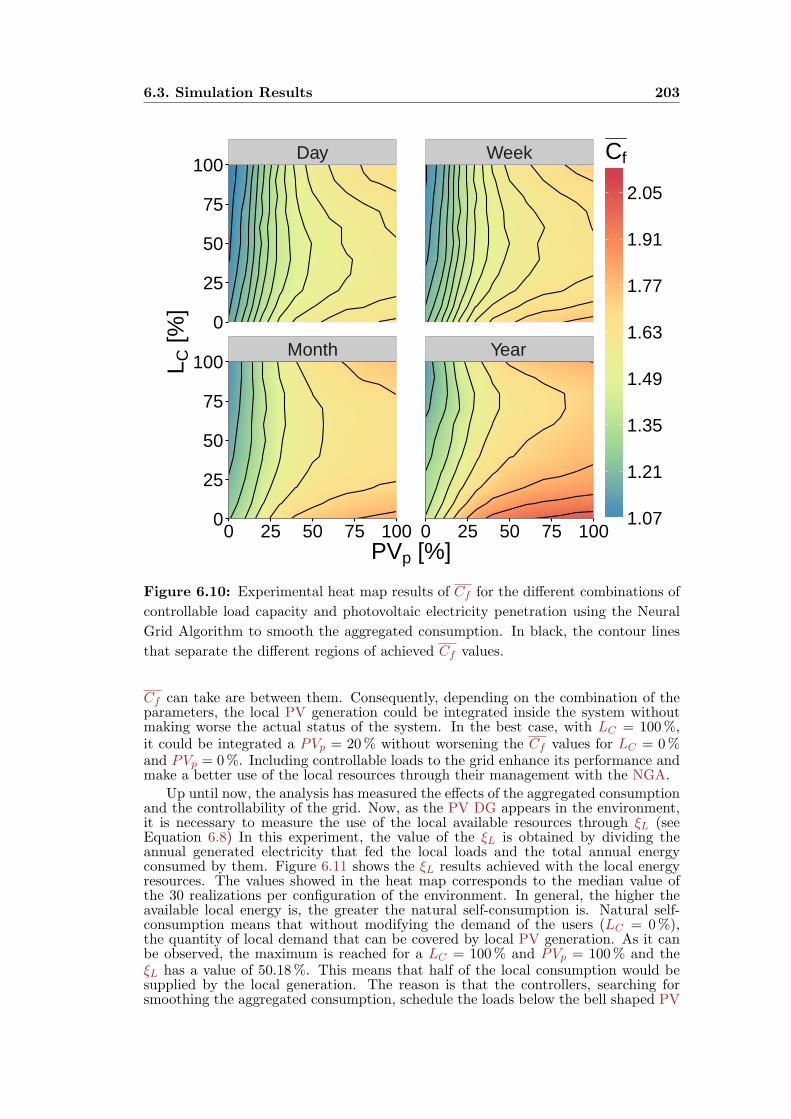
6.3. Simulation Results 203
Day Week
Month Year
0
25
50
75
100
0
25
50
75
100
0 25 50 75 100 0 25 50 75 100PVp [%]
L C [%
]
1.07
1.21
1.35
1.49
1.63
1.77
1.91
2.05
Cf
Figure 6.10: Experimental heat map results of Cf for the different combinations of
controllable load capacity and photovoltaic electricity penetration using the Neural
Grid Algorithm to smooth the aggregated consumption. In black, the contour lines
that separate the different regions of achieved Cf values.
Cf can take are between them. Consequently, depending on the combination of theparameters, the local PV generation could be integrated inside the system withoutmaking worse the actual status of the system. In the best case, with LC = 100%,it could be integrated a PVp = 20% without worsening the Cf values for LC = 0%and PVp = 0%. Including controllable loads to the grid enhance its performance andmake a better use of the local resources through their management with the NGA.
Up until now, the analysis has measured the effects of the aggregated consumptionand the controllability of the grid. Now, as the PV DG appears in the environment,it is necessary to measure the use of the local available resources through ξL (seeEquation 6.8) In this experiment, the value of the ξL is obtained by dividing theannual generated electricity that fed the local loads and the total annual energyconsumed by them. Figure 6.11 shows the ξL results achieved with the local energyresources. The values showed in the heat map corresponds to the median value ofthe 30 realizations per configuration of the environment. In general, the higher theavailable local energy is, the greater the natural self-consumption is. Natural self-consumption means that without modifying the demand of the users (LC = 0%),the quantity of local demand that can be covered by local PV generation. As it canbe observed, the maximum is reached for a LC = 100% and PVp = 100% and theξL has a value of 50.18%. This means that half of the local consumption would besupplied by the local generation. The reason is that the controllers, searching forsmoothing the aggregated consumption, schedule the loads below the bell shaped PV
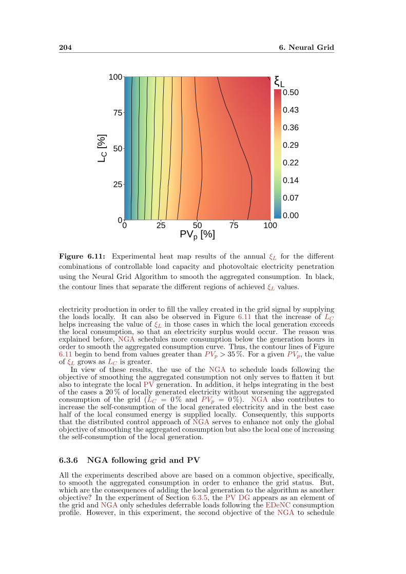
204 6. Neural Grid
0
25
50
75
100
0 25 50 75 100PVp [%]
L C [%
]
0.00
0.07
0.14
0.22
0.29
0.36
0.43
0.50ξL
Figure 6.11: Experimental heat map results of the annual ξL for the different
combinations of controllable load capacity and photovoltaic electricity penetration
using the Neural Grid Algorithm to smooth the aggregated consumption. In black,
the contour lines that separate the different regions of achieved ξL values.
electricity production in order to fill the valley created in the grid signal by supplyingthe loads locally. It can also be observed in Figure 6.11 that the increase of LChelps increasing the value of ξL in those cases in which the local generation exceedsthe local consumption, so that an electricity surplus would occur. The reason wasexplained before, NGA schedules more consumption below the generation hours inorder to smooth the aggregated consumption curve. Thus, the contour lines of Figure6.11 begin to bend from values greater than PVp > 35%. For a given PVp, the valueof ξL grows as LC is greater.
In view of these results, the use of the NGA to schedule loads following theobjective of smoothing the aggregated consumption not only serves to flatten it butalso to integrate the local PV generation. In addition, it helps integrating in the bestof the cases a 20% of locally generated electricity without worsening the aggregatedconsumption of the grid (LC = 0% and PVp = 0%). NGA also contributes toincrease the self-consumption of the local generated electricity and in the best casehalf of the local consumed energy is supplied locally. Consequently, this supportsthat the distributed control approach of NGA serves to enhance not only the globalobjective of smoothing the aggregated consumption but also the local one of increasingthe self-consumption of the local generation.
6.3.6 NGA following grid and PV
All the experiments described above are based on a common objective, specifically,to smooth the aggregated consumption in order to enhance the grid status. But,which are the consequences of adding the local generation to the algorithm as anotherobjective? In the experiment of Section 6.3.5, the PV DG appears as an element ofthe grid and NGA only schedules deferrable loads following the EDeNC consumptionprofile. However, in this experiment, the second objective of the NGA to schedule

6.3. Simulation Results 205
deferrable loads is added. Thus, each controllable node is going to schedule loadsfollowing the EDeNC consumption profile and the forecast of the PV generationweighting the different objectives by the value of β. The node configuration is thesame as in the experiment of Section 6.3.5.
In this case, the capacity of NGA to schedule loads following the antiphaseaggregated consumption and the local generation profiles is tested together with thepenetration of the PV local generation. Therefore, the entire population of nodesis going to be controllable, i.e. LC = 100%. This environment was chosen sincethe algorithm has full actuation capacity over the deferrable loads and its actions willaffect directly the status of the grid. The virtual user is going to create the loads of thenode and defines ∆tui,j to schedule them with NGA respecting the user preferences.In order to schedule the loads, the followed consumption pattern is composed bythe weighted sum of the EDeNC forecast output and the normalized PV generationforecast for the next day. Hence, depending on the β value of the algorithm, it willschedule the loads prioritizing one objective over the other.
As in previous simulations, the number of nodes used during the experiment is600, all equipped with NGA to schedule the loads. The priority of one objectiveagainst the other is varied by changing the value of the β coefficient. In addition, theenergy of the local generators will also vary in order to study the effects of differentPVp levels in the algorithm and the grid. Thus, during the experiment the value ofβ will be varied from 0 (schedule loads to smooth the demand curve) to 1 (scheduleloads to maximize the self-consumption). Whereas the energy of the generators isvaried using the percentage of the PVp from 0% to 100%. So, during the experimentall the possible combinations are scanned to identify the best ones that improve theperformance of the grid and the local self-consumption. The PV generation used isthe Spanish waveform denormalized to the amount of energy indicated by PVp andthe PV generation forecast from the grid operator. For each combination of β andPVp, the experiment has been repeated for 30 seeds to check the repeatability of theexperiment and its statistical validity.
As in the experiment of Section 6.3.5, the only factor analyzed is Cf . This factoris used to evaluate the effects of the NGA and the PV local generation in the statusof the grid. The results of this experiment can be observed in Figure 6.12. TheCf evaluation has been divided in 4 different periods of evaluation, from daily toannually. Then the results are presented in 4 panels, each one corresponding to aheat map for period of evaluation. The color scale is assigned depending on the valueof Cf with respect to β and PVp and it goes from the low values in blue to themaximum values in red. The value of the coefficient represented in Figure 6.12 is themedian of the average performance per period of evaluation for the 30 seeds. As inprevious experiments, the deviation with respect the median is negligible so it is notrepresented.
In general, the behavior observed in Figure 6.12 shows that the variability of theaggregated consumption increases as β and PVp increase their value. In addition, as
both parameters increase, the value of the Cf per period of evaluation is far fromunity and even higher compared to the maximum of Figure 6.10. The reason is thatas the value of β grows NGA will schedule more loads below the generation curveand as the local generator grows in size, the difference between off and on generationperiods produces a bigger variability in the aggregated consumption. With respectto prioritizing one objective against the other, NGA achieves similar values of Cf
for β ∈ [0, 0.5] in all periods of evaluation. However, for β > 0.5, the algorithmgives greater weight to schedule the deferrable loads following the PV forecast whichproduces different values of Cf as PVp grows. The best value of the Cf is obtained bythe algorithm in the absence of DG (PVp = 0%) independent of the value of β sincethere is no local generation. These values are per period of evaluation equal to 1.07daily, 1.09 weekly, 1.11 monthly and 1.13 annually. However, for values of PVp = 0%,
Cf increases and it reaches the highest value for PVp = 100%. In this case, the values
achieved by Cf per period of evaluation are 5.09 daily, 5.18 weekly, 5.23 monthly and5.26 annually. Thus, the grid stability is in danger since the variability presented is

206 6. Neural Grid
Day Week
Month Year
0.00
0.25
0.50
0.75
1.00
0.00
0.25
0.50
0.75
1.00
0 25 50 75 100 0 25 50 75 100PVp [%]
β
1.07
1.67
2.26
2.86
3.46
4.06
4.65
5.25Cf
Figure 6.12: Experimental heat map results of Cf for the different values of
photovoltaic electricity penetration using Neural Grid Algorithm weighting by β its
two objectives: to smooth the aggregated consumption and to maximize the self-
consumption. In black, the contour lines that separate the different regions of achieved
Cf values.
too high. For any other combination of parameters, the value of Cf is between them.However, most of the results have lower values than the worst case. In case of β = 0.5and PVp = 100%, the Cf value per period of evaluation is equal to 1.74 daily, 1.89weekly, 1.99 monthly and 2.30 annually. These values mean an increase of percentageof 62.67% daily, the 73.39% weekly, the 79.27% monthly and the 103.54% annually.60% of the simulated environments are equal or below these values. In this case,NGA could integrate without worsening the grid Cf only a PVp of 10% for β ≥ 0.5,whereas for β < 0.5 a 20%.
On the other hand, the analysis is completed with the study of ξL. It is necessaryto analyze not only the global effects that the variations of β and PVp produce in thegrid, but also the local effects in self-consumption of the local PV generation. ξL iscalculated using the annual local energy generated that supplied the loads and thetotal energy consumed annually. In Figure 6.13, the results of the self-consumptionof the local energy resources are presented. The value of each point of the heat mapis the median value of ξL for the 30 realizations done by each configuration of theparameters. As in the results observed in Figure 6.11, the higher PVp is, the higherthe ξL value is. As can be observed, the increased β value helps to increase the valueof ξL. This value grows until its maximum of ξL= 62.31% reached at a β = 1.0 anda PVp = 100%. Thus, comparing the maximum achieved in this experiment and the
6.3. Simulation Results 207
0.00
0.25
0.50
0.75
1.00
0 25 50 75 100PVp [%]
β
0.00
0.09
0.18
0.27
0.35
0.44
0.53
0.62ξL
Figure 6.13: Experimental heat map results of the annual ξL for the different values
of photovoltaic electricity penetration using the Neural Grid Algorithm weighting by
β its two objectives: to smooth the aggregated consumption and to maximize the
self-consumption. In black, the contour lines that separate the different regions of
achieved ξL values.
one obtained in the experiment of Section 6.3.5, the increase of ξL was of 12.13%by using the PV forecast to schedule the loads. In general, the increase of the βvalue helps increasing ξL. In Figure 6.13, for PVp > 25% the surplus of generatedPV electricity is better used as the value of β is increased. That is the reason whythe contour lines present an exponential form from this value of PVp. For previousvalues, the contour lines of ξL are linear and do not suffer any variation since thereis no surplus of generated electricity and it is covered totally by the loads.
To sum up, the use of NGA to schedule the loads following the two objectivesweighted by β does not only entail an increase of the self-consumption but also anincrease of the variability of the aggregated consumption. So depending on the target,the value of β can be used to give more weight to one decision versus the other. Inview of the results, it has also been stated that the two objectives of the NGA areconflicting since the increase of the self-consumption decreases the smoothing of theaggregated consumption. For high values of β and PVp, Cf is far from the unity butmore than the 60% of the consumption is supplied locally. Thus, a better solution hasto be found in order to increase the self-consumption without influencing negativelythe aggregated consumption waveform.
6.3.7 NGA with DER
As already shown, adding the second objective to the NGA favors the self-consumption but the variability of the signal is increased. This fact has forcedto rethink the use of the algorithm since in situations with high amount of localPV electricity generation, the algorithm produces non-desirable effects in the griddepending on the priority of the objectives. The increased variability occurs mainly
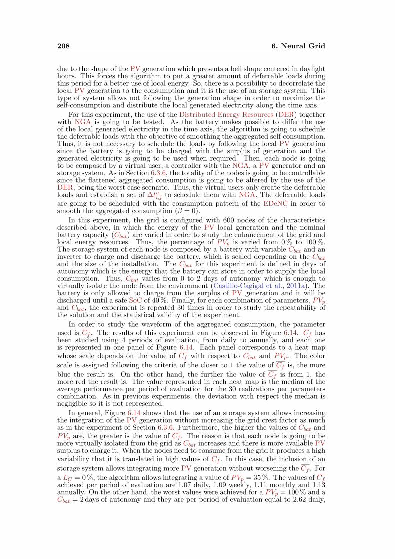
208 6. Neural Grid
due to the shape of the PV generation which presents a bell shape centered in daylighthours. This forces the algorithm to put a greater amount of deferrable loads duringthis period for a better use of local energy. So, there is a possibility to decorrelate thelocal PV generation to the consumption and it is the use of an storage system. Thistype of system allows not following the generation shape in order to maximize theself-consumption and distribute the local generated electricity along the time axis.
For this experiment, the use of the Distributed Energy Resources (DER) togetherwith NGA is going to be tested. As the battery makes possible to differ the useof the local generated electricity in the time axis, the algorithm is going to schedulethe deferrable loads with the objective of smoothing the aggregated self-consumption.Thus, it is not necessary to schedule the loads by following the local PV generationsince the battery is going to be charged with the surplus of generation and thegenerated electricity is going to be used when required. Then, each node is goingto be composed by a virtual user, a controller with the NGA, a PV generator and anstorage system. As in Section 6.3.6, the totality of the nodes is going to be controllablesince the flattened aggregated consumption is going to be altered by the use of theDER, being the worst case scenario. Thus, the virtual users only create the deferrableloads and establish a set of ∆tui,j to schedule them with NGA. The deferrable loadsare going to be scheduled with the consumption pattern of the EDeNC in order tosmooth the aggregated consumption (β = 0).
In this experiment, the grid is configured with 600 nodes of the characteristicsdescribed above, in which the energy of the PV local generation and the nominalbattery capacity (Cbat) are varied in order to study the enhancement of the grid andlocal energy resources. Thus, the percentage of PVp is varied from 0% to 100%.The storage system of each node is composed by a battery with variable Cbat and aninverter to charge and discharge the battery, which is scaled depending on the Cbatand the size of the installation. The Cbat for this experiment is defined in days ofautonomy which is the energy that the battery can store in order to supply the localconsumption. Thus, Cbat varies from 0 to 2 days of autonomy which is enough tovirtually isolate the node from the environment (Castillo-Cagigal et al., 2011a). Thebattery is only allowed to charge from the surplus of PV generation and it will bedischarged until a safe SoC of 40%. Finally, for each combination of parameters, PVpand Cbat, the experiment is repeated 30 times in order to study the repeatability ofthe solution and the statistical validity of the experiment.
In order to study the waveform of the aggregated consumption, the parameterused is Cf . The results of this experiment can be observed in Figure 6.14. Cf hasbeen studied using 4 periods of evaluation, from daily to annually, and each oneis represented in one panel of Figure 6.14. Each panel corresponds to a heat mapwhose scale depends on the value of Cf with respect to Cbat and PVp. The color
scale is assigned following the criteria of the closer to 1 the value of Cf is, the more
blue the result is. On the other hand, the further the value of Cf is from 1, themore red the result is. The value represented in each heat map is the median of theaverage performance per period of evaluation for the 30 realizations per parameterscombination. As in previous experiments, the deviation with respect the median isnegligible so it is not represented.
In general, Figure 6.14 shows that the use of an storage system allows increasingthe integration of the PV generation without increasing the grid crest factor as muchas in the experiment of Section 6.3.6. Furthermore, the higher the values of Cbat andPVp are, the greater is the value of Cf . The reason is that each node is going to bemore virtually isolated from the grid as Cbat increases and there is more available PVsurplus to charge it. When the nodes need to consume from the grid it produces a highvariability that it is translated in high values of Cf . In this case, the inclusion of an
storage system allows integrating more PV generation without worsening the Cf . For
a LC = 0%, the algorithm allows integrating a value of PVp = 35%. The values of Cfachieved per period of evaluation are 1.07 daily, 1.09 weekly, 1.11 monthly and 1.13annually. On the other hand, the worst values were achieved for a PVp = 100% and aCbat = 2days of autonomy and they are per period of evaluation equal to 2.62 daily,
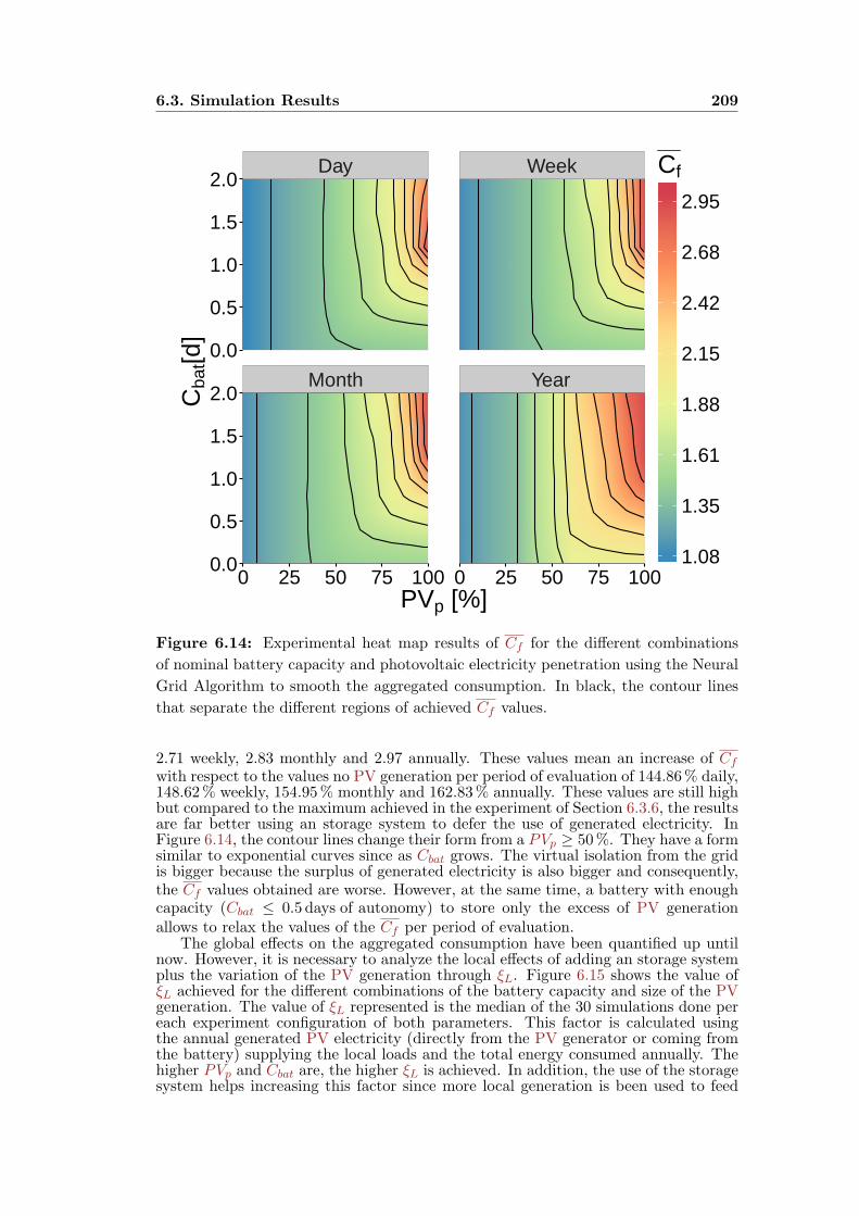
6.3. Simulation Results 209
Day Week
Month Year
0.0
0.5
1.0
1.5
2.0
0.0
0.5
1.0
1.5
2.0
0 25 50 75 100 0 25 50 75 100PVp [%]
Cba
t[d]
1.08
1.35
1.61
1.88
2.15
2.42
2.68
2.95
Cf
Figure 6.14: Experimental heat map results of Cf for the different combinations
of nominal battery capacity and photovoltaic electricity penetration using the Neural
Grid Algorithm to smooth the aggregated consumption. In black, the contour lines
that separate the different regions of achieved Cf values.
2.71 weekly, 2.83 monthly and 2.97 annually. These values mean an increase of Cf
with respect to the values no PV generation per period of evaluation of 144.86% daily,148.62% weekly, 154.95% monthly and 162.83% annually. These values are still highbut compared to the maximum achieved in the experiment of Section 6.3.6, the resultsare far better using an storage system to defer the use of generated electricity. InFigure 6.14, the contour lines change their form from a PVp ≥ 50%. They have a formsimilar to exponential curves since as Cbat grows. The virtual isolation from the gridis bigger because the surplus of generated electricity is also bigger and consequently,the Cf values obtained are worse. However, at the same time, a battery with enoughcapacity (Cbat ≤ 0.5 days of autonomy) to store only the excess of PV generationallows to relax the values of the Cf per period of evaluation.
The global effects on the aggregated consumption have been quantified up untilnow. However, it is necessary to analyze the local effects of adding an storage systemplus the variation of the PV generation through ξL. Figure 6.15 shows the value ofξL achieved for the different combinations of the battery capacity and size of the PVgeneration. The value of ξL represented is the median of the 30 simulations done pereach experiment configuration of both parameters. This factor is calculated usingthe annual generated PV electricity (directly from the PV generator or coming fromthe battery) supplying the local loads and the total energy consumed annually. Thehigher PVp and Cbat are, the higher ξL is achieved. In addition, the use of the storagesystem helps increasing this factor since more local generation is been used to feed
210 6. Neural Grid
0.0
0.5
1.0
1.5
2.0
0 25 50 75 100PVp [%]
Cba
t[d]
0.00
0.11
0.23
0.34
0.46
0.57
0.69
0.80ξL
Figure 6.15: Experimental heat map results of the annual ξL for the different
combinations of nominal battery capacity and photovoltaic electricity penetration
using the Neural Grid Algorithm to smooth the aggregated consumption. In black,
the contour lines that separate the different regions of achieved ξL values.
locally the consumption. The minimum value obtained is ξL= 0% which is achievedwhen no local generation is available. Whereas the maximum ξL is achieved at the endof the experiment for a Cbat = 2days of autonomy and PVp = 100% and it is equalto 79.98%. Comparing to the maximums achieved in the experiments of Sections6.3.5 and 6.3.6, it implies an increase of 29.80% and 17.67%, respectively. Thus, thestorage system allows a better use of the local resources as shown by the contour linesof Figure 6.15. Furthermore, the use of an storage system does not only benefit thelocal self-consumption, but also globally, it allows integrating a higher percentage ofPV generation and decreases the Cf of the grid, as if the loads were consuming allthe local electricity generated at the same time that it is produced.
In conclusion, this experiment shows that adding an storage system to the node isa better option in order to increase the self-consumption of the local resources and notincreasing in excess the variability of the aggregated consumption. The storage systemallows consuming the PV electricity not only at generation hours, so that relativelylow Cbat that absorbs the surplus of the PV enhance the system both locally andglobally. In addition, even with higher values of PVp, it has been reduced the effectsseen in Section 6.3.6 but the variations introduced are still too high. However, thestorage system allows bigger quantities of PV generation inside the grid, PVp ≤ 35%,and it achieves that 80% of the consumption can be fed locally.
6.4 Summary and discussion
In this Chapter the EDeNC response, developed in Chapters 4 and 5, was testedin a simulated environment which resembles a real grid. For this purpose, the

6.4. Summary and discussion 211
GPLV3.0 open simulator GridSim4 was used as a tool to develop all the analysisand experiments. GridSim is a powerful tool that simulates the power flows of anelectrical grid and models different elements inside the grid that resembles the realones. In this case, the facilities used during the simulations were composed by threeelements: consumption, local PV generation and an storage system. The consumptionis formed by the three types loads: deferrable, non-deferrable and elastic. Thus, thedirect application of the EDeNC is complex inside this environment. In addition,with the appearance of local energy sources, a new objective was posed in order toenhance its local use.
In this scenario, the proposed algorithm in this Thesis has been completedand validated according to two objectives: one global, smoothing the aggregatedconsumption of a grid, and one local, maximizing the self-consumption of the localenergy resources. This proposed algorithm, called Neural Grid Algorithm (NGA),was developed based on the use of the response of the EDeNC and the PV DG thatthe facilities incorporate. In order to achieve the first objective, the NGA uses theproperties of the EDeNC to reduce the variability of a signal, which correspondsperfectly to the objective of smoothing the aggregated consumption of a grid. On theother hand, the second objective of the NGA needs to include information relativeto the local generation in order to decide when the facility should consume and takeadvantage of it. Therefore, the NGA incorporates the forecast of the day ahead forthe local PV generator. Both objectives are weighted by a β coefficient in order togive different priority to the objectives.
NGA actuates over the demand of the facility based in these objectives. TheEDeNC response is prepared to actuate directly over the power of the facility, howeverin a real environment a few consumptions can be modified directly. Hence, the NGAused the consumption profiles of both objectives in order to schedule the differentloads of the user. Then, the consumption has been discretized in energy packages thatrepresent the loads of a facility and depending on the grade of the controllable loadcapacity (LC), the algorithm has more energy to defer following the two objectives.These energy packets are created by a virtual user which uses a consumption profileto schedule them in probability. It is the virtual user which establishes the amount ofenergy that it is deferrable, non-deferrable or elastic. Thus, the NGA would actuateover the activation time of the deferrable loads respecting the user preferences andscheduling them by the use of a probability density function based on the weightedsum of the two objectives of the algorithm.
Once the definition of the algorithm has been introduced, five different experimentswere designed in order to test it. Each of them tests different aspects of the algorithm.The first one tests the direct use of the EDeNC response with elastic loads over thegrid by varying LC . The second one test the load scheduling capacities of the NGAin order to smooth the aggregated consumption by varying LC . In the third one,the PV DG was added to the facilities to test the integration of the PV generationwhen the NGA only schedules loads based on the first objective. In this case, LCand photovoltaic electricity penetration (PVp) were varying. The fourth experimentstudies the full capabilities of the NGA in order to schedule the loads based on thetwo objectives. In this case, LC was equal to 100% and β and PVp were varied.Finally, the last experiment, following the results of the previous one, used an storagesystem together with the PV generation in order to enhance the grid status. In thisexperiment, the NGA was used to schedule loads with the objective of smoothing thedemand since the properties of the storage systems were tested. LC was equal to 100%and Cbat and PVp were varied. In the first two experiments, the analysis consisted of
studying the average crest factor (Cf ), average load factor (Lf ) and average demand
factor (Df ) to quantify the effects on the grid. Whereas in the rest of the experiments
Cf and self-consumption normalized by the consumption (ξL) were studied to analyzethe effects on the grid and quantify the local use of the DER.
As a general remark, the inclusion of LC with the NGA improves the grid statusthrough the reduction of the variability of the aggregated consumption and alsoimproves the use of available resources. In case of using elastic loads, it is needed
4Source: https://github.com/Robolabo/gridSim

212
a 30% of LC to achieve an annual reduction of the variability of 30%. Whereasusing the algorithm to recommend the user when is the best time to activate thedeferrable loads, it is needed an LC = 50% to at least reduce annually the variabilityin a 13%. In addition, the NGA presents some errors due to the discretization ofthe consumption and the use of the forecast response of the EDeNC. Furthermore,the use of the NGA following only the first objective allows a better integration ofthe PV DG as LC increases. But, it allows that for values of PVp less than 20%the grid status does not get worse and the maximum ξL achieved is of 50%. At thesame time, the NGA allows enhancing the self-consumption of the facility increasingthe use of the local energy sources. With respect to the two objectives of the NGA,prioritizing the second objective produces a higher variability on the grid but at thesame time higher values of ξL are achieved around 60%. For values of β ∈ [0, 0.5] thealgorithm is able to maintain relatively similar variabilities in the grid and achieves ahigh use of the local resources. Finally, the inclusion of an storage system relaxes theconstraints of the environment and allows consuming the generated electricity whenit is needed. Thus, with an storage system, the PVp achieved is of 35% and at thesame time reduces the variabilities achieved by scheduling loads following the NGAobjectives. In addition, the use of the local energy resources is improved and reachesa value of the 80%.

PART III
Conclusions

7Conclusions and Future Works
“Stay hungry. Stay foolish” — Rashmi Bansal
Key features of a self-organized coordination algorithm to manage thepower flows of an electrical grid have been presented in this Thesis.The aim of the Thesis was the application of Artificial Intelligence(AI) algorithms, specifically Recurrent Neural Networks (RNNs), to
the distributed control of a grid with the presence of Distributed Energy Resources(DER). In this last Chapter, the main achievements and remarks of the Thesis aresummarised, both in the computer science and energy fields. The remainder ofthe Chapter is as follows. Section 7.1 presents an overview of the developments,improvements and results obtained within the objective proposed in the presentThesis. Section 7.2 presents different application possibilities of the results of thisThesis and some proposals to develop in future research. Finally, Section 7.3summarizes the main contributions of the author over the course of fulfilling thisdissertation.
7.1 Conclusions
The present structure of the electrical grid has not suffered disruptive changes sinceits creation in the XIX century. However, its evolution has become essential as somefactors are threatening its stability such as the growing demand, while others are beingrecently developed inside it without their proper integration such as Information andCommunications Technology (ICT) or Distributed Generation (DG). The emergenceof DG supposed a change of paradigm in the structure of the grid, since the generationis closer to the places where it is consumed, enhancing the local system status.Furthermore, the degree of connectivity between the different grid elements has beenincreased thanks to ICTs, being necessary to process all the data gathered in order toenhance the grid operation. The present Thesis sheds light on the problems arisingfrom the management and operation of existing electrical grids and their evolution towhat is considered the grid of the future or Smart Grid (SG).
The SG has arisen from the convergence of five key aspects that all the definitionshave in common: i) the grid, ii) ICTs, iii) renewable energies, iv) Electrical EnergyStorages (EESs) and v) Demand Side Management (DSM). In this Thesis, a definitionof the SG has been suggested to explain the meaning of this huge concept and tounderstand what would the next generation of grids become. Thus, in the frameworkof the present Thesis, a SG is considered as an electricity network that uses the ICTs tocoordinate the needs of all groups inside the system to operate all its parts as efficientlyas possible, minimizing costs and environmental impacts while maximizing systemreliability, resilience and stability. The SG presents benefits for all the members ofthe grid (security of supply, reliability, efficient, etc.), and also for the environment.SG is still at an early stage to be deployed and a lot of research has to be done beforeits final stage arises. However, it also faces a lot of barriers to be fully adopted, butthe most worrying problem is the lack of investment to carry out the development ofthese technologies.

216 7. Conclusions and Future Works
This Thesis consists of a first step towards the SG by linking and integratingthe five key aspects for its development and deployment in the near future. To thisend, an algorithm is proposed to process the tones of data that the ICTs gatherin order to benefit all the parts of the grid. Greater operational efficiency, costreductions and reduced risks are achieved. The current centralized structure of thegrid does not favor the information processing as the data load is large enough totake decisions by the operators. Thus, the proposed algorithm follows a decentralizedapproximation in order to alleviate the data load of the centralized node. In thisscenario, the decentralization was taken to the end of the grid, making the usersparticipants in their decisions and being able to manage their power flows into acommon objective, increasing the sustainability of the system, through DER andan efficient use of electricity generated. The proposed algorithm is based on DSMtechniques combined with an automatic control of demand that helps to integrateDER (renewable energies and EES), which leads to an innovative concept called ActiveDemand Side Management (ADSM). This ADSM algorithm serves as the cohesiveelement that links all the elements that define the SG.
Among all the possibilities to implement an ADSM algorithm, the proposal ofthe Thesis is based on one of the famous algorithms coming from the field of the AI,the Artificial Neural Networks (ANNs). They have been studied since the 50s, butit was during the 80s that almost all the developments were done. Some problemswere found during this time, but they were overcome and nowadays they enjoy ofa fame well deserved thanks to their properties. As the ADSM algorithm is goingto be used in large scale and changing environment, ANNs were selected for theirproperties of adaptivity, generalization, redundancy, fault tolerance and distributivity,among others. In addition, the modularity of ANN offers the possibility to divide acomplex problem into easier tasks that help to solve the global problem. All theproperties that the ANN possesses are similar to the ones that the future SG willprovide to conventional power systems. There exist plenty of ANN types, but forthe proposed algorithm there are two fundamental attributes that must be targeted,the time variable and the presence of memory. So, the type of ANNs selected is theRNNs, specifically the Continuous Time RNNs (CTRNNs) since it includes all thoseproperties in its structure plus dynamic features that help in a changing environment.
The objective of the proposed ADSM algorithm is to enhance the performance ofthe grid. To this end, the local consumption is managed to reduce the variability ofthe aggregated consumption producing an smoothed signal and at the same time italso responds to local conditions. The ADSM strategy followed is applied locally butits effects impact globally in the system. Therefore, it is necessary to involve users inthis process and the coordination between facilities and the grid should be performed,where a facility is owned by a particular consumer whose management dependson him and is composed by Photovoltaics (PV) generation, an storage system andconsumption. However, the coordination process is done without any communicationamong the users. Thus, the only information available to coordinate the ensembleof users is the aggregated consumption of the grid. Data protection and anonymityis guaranteed following this approach. Consequently, the different users inside thegrid are self-organized to contribute to smooth their aggregated consumption. Tothis extent, the CTRNN was used to control the local electric behavior taking intoaccount the aggregated consumption of the electrical grid, local energy resources andusers requirements.
In the implementation of the ADSM, it was crucial the use of the CTRNN becauseits signal processing and forecasting abilities make particularly interesting their usein a changing environment as the grid. In addition, the dynamic properties and theshort-term memory of its structure helped to create an approximation to reduce thevariability of a signal. The aggregated consumption is a complex signal which dependson the behavior of all users connected to the grid. However, this signal presents somecharacteristics that helps to identify an approach to flatten it. Among its features,it presents that it is continuous, periodic, bounded and differentiable of class C1.Thus, taking into account these signal features, a CTRNN controller is built to cancelthe derivative of the aggregated consumption achieving a constant aggregated signal.Consequently, the controllable users build a destructive interference through their
7.1. Conclusions 217
consumption that it is in antiphase to the one corresponding to the non-controllableusers and as a result, the aggregation of all the consumptions will generate a smoothaggregated consumption.
However, it was necessary to define the structure of the CTRNN to be able tocancel the derivative of the input aggregated signal coming from the environment.During the selection of the architecture some considerations were taken about its sizesince large CTRNNs are difficult to analyze and computationally slow. Thus, smallstructures were explored in order to be able to use them together with any technologyinside any type of user facility. At the same time, a modular approximation wasfollowed consisting of neural blocks where each one solves parts of the problem. Inorder to find the right structure of the neural controller, a second algorithm wasused to tune its synaptic weights, the Genetic Algorithm (GA). During the searchof the best structures, not only different parameters of the neural controller wereadjusted but also an analysis of the best configuration of the GA was carried out inorder to understand the influence of its parameters in the search of the best solution.The GA evaluated the capacity of the evolved structure to cancel the variabilityof the input signal through the extraction of its derivative and the consumption ofan antiphase output. To this end, 388, 800 simulations were carried out for all thedifferent neural structures. The best structure found was the one formed by an inputlayer of 2 neurons, a hidden layer of 4 neurons and an output layer of 1 neuron. Theinformation goes feedforward between layers, each neuron presents a feedback loopwith itself and the ones of the hidden layer present feedback loops among them. Inaddition, there is a feedback loop from the output to the input, so the network canstore its last actuation. A post-evaluation was done to analyze the response of theevolved neural controller and for all the tested signals, a variability reduction of theinput signals between the 60% and the 16% was achieved.
The evolved neural controller is the central block of the ADSM controller. How-ever, its direct application in the grid could not be done since all users will consumethe same and the grid is composed by an heterogeneous environment. Moreover,if all users try to consume the same power at the same time, greater variabilitiesof the aggregated consumption are reached. Thus, a coordination algorithm wasimplemented in order to produce collectively the antiphase consumption necessary toflatten the aggregated consumption. Inspired in the Blind Source Separation (BSS)techniques, the τ -Learning Algorithm (τLA) was used to regulate the output of theneural controller ensemble based on the last free parameter of the network, the timeconstant (τi). This parameter is related with the reaction speed of the neurons.The τLA was implemented following a reinforcement learning paradigm in which theminimization of the variability of the aggregated environment signal is used to changethe value of this parameter. The use of the τLA implies that after the evolution, eachevolved neural controller was developed to obtain its own output different from themajority of controllers. With this achievement, the birth of the Evo-Devo NeuralController (EDeNC) arose to control the local demand of a user. The EDeNC couldbe used in two modes of operations: adapting to the environment with or withoutpower constraints. In both cases, an smoothed aggregated environment signal isachieved from a neural distributed way.
Finally, the direct use of the EDeNC is not recommended as it actuates directlyover the power of the user and there are a few loads that allows this behavior. Inaddition, local Distributed Energy Resources (DER) considerations are not takeninto account in the EDeNC. Thus, the proposed algorithm, which is implementedas an ADSM controller, uses the response of the EDeNC and a local PV generationforecast to elaborate a consumption pattern of the user. This algorithm or Neural GridAlgorithm (NGA) has two objectives: one global, the smoothness of the aggregatedconsumption and one local, the maximization of the local energy resources use.Both objectives are weighted by a β coefficient to establish different priorities inthe objectives. Then, the consumption pattern generated by the NGA is used toschedule the different deferrable loads that the user possesses. The algorithm wastested in a virtual environment for selected scenarios closer to reality. The dataused in the simulations were the total PV generation forecast of one day ahead,the total PV generated and the aggregated consumption of the Spanish peninsulargrid in 2015. As a general remark, the inclusion of the loads controllable fraction,
218 7. Conclusions and Future Works
LC , with the NGA improves the grid status through the reduction of the aggregatedconsumption variability plus a better use of the available energy resources. It is neededan LC = 50% to at least reduce annually the variability in a 13%. In addition, the useof the algorithm allows integrating the local PV generation for photovoltaic electricitypenetration (PVp) less than 20% without worsening the status of the grid. The useof local storage allows a bigger integration (PVp ≤ 35%) and a higher use of the localenergy is achieved. As conclusion, the algorithm was able to adapt the controllabledemand to the non-controllable one and thanks to its use, the NGA reduced the yearlyvariability of the aggregated consumption. Thus, the NGA meets the main objectivesought in this Thesis.
To conclude, the use of the NGA developed in this Thesis entails an importantcontribution to the deployment of the future SG. With its implementation, someneeds and barriers referred in Sections 2.2 and 2.3 were tackled. The benefits thatintroduced the use of the NGA are summarized as follows:
The efficiency of the system is increased with the reduction of the peaks as lesspower is demanded instantaneously. The use of the NGA also helps to decreasethe oversizing of the electric system in order to guarantee the supply. And italso helps the grid operators with their daily tasks such as the scheduling of thegeneration for the next day, integrating some forms of energy, etc.
Increasing the robustness as the redundancy of infrastructures inside the grid isincreased. As a distributed algorithm, if one of the facilities fails, the remainingfacilities will adapt their consumption to continue smoothing the aggregatedconsumption. In this case, the distributed property of the algorithm is doubled,not only at the facility level but also the EDeNC presents this property insidethe facility. In addition, the robustness is also increased since the essentialinformation is sent from the nodes to the grid and vice versa. Compromisingthe information through the ICTs is more difficult due to the reduction of nodecommunications.
Data privacy is assured since no communication between the nodes is availablewith the algorithm.
Reduced computational load. As all the decisions are made from the side of theuser, the computational load of processing and making decisions is not as highas if a central node was in charge of doing all these operations. Moreover, thesimplified structure of the EDeNC makes possible its execution in any currenttechnology since the computational effort is not huge.
Reduced investments and costs with the use of NGA since it adapts to thecurrent status of the grid. Some modifications are still required such asthe upgrade of the sensory platform in order to establish a double-sidedcommunication. However, it is not necessary that each node possesses highcomputational power or any other sophistication, since only providing the formof the aggregated consumption will be enough to deploy the NGA and takebenefit for all its features.
7.2 Future Work
This Thesis is the NGA mark I. Although a first approximation of the future SGwas achieved with this algorithm, further development is required in order to improveits performance. In this Thesis, a combination of the Artificial Intelligence (AI) andthe energy management fields were found. During the development of this Thesis,different research lines have been identified for future exploration that would beinteresting to study.
The algorithm developed in this Thesis is still in a first version of its development.Furthermore, the NGA is not mature enough for its deployment at large scale in real
7.2. Future Work 219
grids, but it could be used in reduced environments, such as buildings or microgrids.However, some improvements should be made in order to use its final implementationin real environments. These improvements are listed as follows:
Improve the prediction horizon. One of the problems found with the NGA tosmooth the aggregated consumption is the scheduling of the loads with the realtime operation of the EDeNC. The EDeNC was able to predict one step aheadto cancel the derivative of a signal and thanks to the periodicity of the signalit was able to achieve its purpose. However, the period of repeatability wasof one week being too much time for the algorithm if some unexpected eventhappens. Thus, increasing the forecasting capabilities of the EDeNC wouldincrease the performance of the algorithm and unexpected events would betaken into account. To do so, following the task partitioning approximationby dividing the problem into simpler parts, a specific prediction module couldbe added to the current form of the EDeNC. Hence, the EDeNC would notbe modified and this new module could be as complex as it is required toelaborate the prediction of the aggregated consumption. On the other hand,another possibility would consist of the modification of the EDeNC structureby increasing the history and using more outputs corresponding to the differenttime steps of the forecast. In this way, it would be necessary that the structureof the EDeNC would follow a Nonlinear Autoregressive Moving Average witheXogenous inputs (NARMAX) approximation. Apart from these two types ofapproximations, a third way can be used to increase the prediction horizon.Changing the neural structure could also be helpful. For example, the useof Long Short Term Memory (LSTM) networks would help to increase theforecasting capabilities without compromising the neural structure. LSTMnetworks are a type of RNN which learn from experience to classify, processand predict time series when there are important long time lags of unknownsize between events.
User consumption profiles. In this Thesis, a virtual user was in charge of creatingloads with respect to a consumption profile. However, only elastic and deferrableloads were used separately to show the characteristics of the EDeNC and NGA,respectively. A more complex consumption profile could be achieved if the threetypes of loads defined in this Thesis (non deferrable, deferrable and elastic) wereused together and assigned by the virtual user. In this way, a more realisticdemand profile per user should be simulated and the strategy of scheduling loadsby the NGA should be reconsidered. The control capacity of the NGA shouldbe increased in order to be able to manage the three types of loads added. Forthe non-deferrable loads, the algorithm has to ignore them since they are goingto be executed when the virtual user needs them. The scheduling capacitiesof the NGA are still valid, however the algorithm has to take into accountnot only the deferrable energy packages but also the direct power load controlover the elastic ones. In addition, the specifications of the elastic loads aredifferent from the deferrable ones since each one presents different features: forexample, the Electric Vehicle (EV) is a mobile load that can also be used asan storage system and the Heating, Ventilation and Air Conditioning (HVAC)loads maintain a comfort temperature ordered by the user. Deferrable loadscould also increase their realistic form if the real consumption profiles of theseloads were implemented. In this Thesis, only the end user consumption profilewas used based on the residential sector. However, different types of usershave to be integrated in the system to give more realism to the virtual gridenvironment, e.g. industrial or commercial users, as other special loads that thegrid operators use.
Multi purpose algorithm. The NGA presented in this Thesis is composed bymore than one objective. However, both targets were antagonistic and theincrease of one of them will imply the decrease of the other. A better integrationof the two objectives was done with the addition of an storage system in theenvironment but it was not part of the algorithm. Therefore, adding the storage
220 7. Conclusions and Future Works
system as part of the algorithm could suppose a great asset as both objectivesare better integrated and the algorithm achieves better performance. Moreover,storage systems are increasingly used due to their value in terms of flexibility,technological improvements of the different technologies, the appearance of newsolutions from different companies and the emergence of the EV. The paradigmof the storage systems has been changing since the introduction of the EVbecause the storage system is not static anymore, it is mobile. The peculiarityof the EV is that it can be used as a load or as a storage system, always takinginto account not only the energy requirements of the user but also their mobilitycapacity, as it can be connected in any part of the grid. For example, the userneeds the vehicle to move from home to another place in which is going to do anactivity, during those periods of time that the EV is not used, the NGA could useit to charge or discharge the battery following the user requirements and takinginto account when it is going to be used again. This behavior complicates thedecisions that the algorithm has to take in order to achieve its objectives. Butit also gives the opportunity to a new field of research to reduce the variabilitiesof the aggregated consumption in a concrete area.
Complete neural system. The consumption pattern generated by the algorithmwas weighted by the β coefficient. This method serves to establish differentpriorities for the objectives of the algorithm and achieve good results with theintegration of both objectives. However, the decisions were made using nonneural elements. In order to get a better performance, a good way to integrateboth objectives is the use of a complete neural system to decide the consumptionpattern. This modular neural system would respond to different objectivesgenerating only one response in which all the targets are integrated. As oneof the major applications of the ANN is the classification and decision making,creating a whole neural system, it is unavoidable to increase the performanceof the algorithm. Thus, a first approximation would be using the EDeNCresponse plus the PV forecast as inputs to an ANN that selects the betterobjective each time. Adding new objectives (electrical savings) or new elements(storage systems) into the system will consist of adding more inputs to theneural decision-making block, but the training would include all these newtargets and elements in order to obtain the required results. Furthermore,for a complete neural system, the PV forecasting can also be done by usingan ANN. This predictive module would help to elaborate predictions locallywhich are essential coordinating the different regions that compose the grid.A disadvantage of getting a large scale neural model is the complexity of thetraining for each module and the computation capacity of the nodes. But oncethe right direction of implementing a solution is found, it is the best way toincrease the whole performance.
More forms of generation. The most widespread technology used in DG isPV. This is also the form of local generation used for the development of thealgorithm proposed in this Thesis. However, there exist other DG technologiesamong which are multiple renewable energy technologies. One of the mostpopular forms of DG together with PV is the use of wind power generation.Its integration in the current form of the algorithm is very easy and it can bedone in three different ways: substituting the PV, adding a new coefficient toprioritize one local resource or the other, or directly in the generation forecastby adding its response to the one of the PV. Hence, the NGA will continuesmoothing the aggregated consumption at the same time that tries to maximizethe self-consumption of one or more forms of local generation. In spite of thefast integration in the system, wind power presents a high variability of theresources since its availability is not controllable.In addition, getting closer to a real environment, the virtual grid couldincorporate different forms of generation typical from the actual grid, such asnuclear power plants or hydraulic ones in order to correlate the matching of theconsumption and the generation. By adding different forms of generation, thecorrelation of the decisions made by the algorithm and the capacity of the system

7.2. Future Work 221
to respond to them will also be tested. The complexity of the environmentoffers an opportunity to study the different effects that can happen with theapplication of this type of algorithms.
Spatial simulation grid configuration. During this Thesis, the aggregatedconsumption is done instantaneously without taking into account the placeswhere the electricity generated comes from or the different sites where theconsumption occurs. As no spatial considerations were taken, the losses aroundthe transportation of electricity could not be taken into account or estimatedin the aggregation of the consumption. Therefore, quantification of savingsand losses introduced with the NGA could serve to its final deployment in thecurrent grids. This study would also serve as a measurement to improve theconflicting points of the algorithm in the interaction of the facility with the grid.In addition, the inclusion of the spatial dimension to the problem would serveto understand better the effects of the DG and quantify the benefits of usingit with respect to the generated electricity coming from the grid. Some specialconfigurations could also be simulated like the island operation of a group offacilities or some microgrids with shared resources. Finally, this study couldserve to design and sizing the equipment needed in the grid for the applicationof the NGA to its future deployment in the SG.
These are some improvements that could be implemented for a fully operationalalgorithm to be used inside the SG. However, at the same time there exist otherapplications in which the developments achieved in this Thesis could also be used.Some of these applications are also related with the energy field whereas otherapplications are related with the signal processing capabilities of the algorithm. Theseapplications are as follows:
Microgrid management1. During the development of the evolved neuralcontrollers, the adaptation capabilities of the controllers were tested in a reducedenvironment in which new users have to adapt their consumption profile tothe one of the environment. The use of this property of the EDeNC is veryconvenient to manage the different consumptions inside microgrids for theoptimization of the resources. The idea is that through the self-organizationcapabilities of the EDeNC, the users are able to optimize the use of the localresources minimizing the interactions with the grid. There exist some limitationsinside the microgrid that the EDeNC could use in order to share all the resourcesamong the different users. Moreover, the EDeNC could be used to adapt theconsumption of some users to other ones that have priority over the rest, sono energy resource is wasted. In addition, not only the consumption insidethe microgrid can be optimized with the EDeNC, the combination of differentmicrogrids could also be coordinated with the use of the NGA.
Load shedding. With the growth of the EV in the transportation sector, a newconcern has arisen with respect to the infrastructures to charge its battery.Imagine that inside a garage of a block of flats, all the neighbors have an EV.The parking spot of each neighbor will be equipped with a charger for its vehiclebut the common installation of the garage will probably not be changed sincethe construction of the building. In the case that all the cars need to be chargedat the same time, a peak of current is demanded that would soon overload thecapacity of the infrastructure. For this reason, different approaches are used toshed the load of the different EVs of the garage. However, this will disconnectthose loads that are not considered primary in the system, so some cars willnot be charged while the power demanded is reduced. It is in this scenariothat the use of the EDeNC could be beneficial in order to regulate the currentused to charge the batteries of the cars. Using the EDeNCs, all the EVs couldbe charging but not at the maximum current of the installation since it will
1A microgrid is a localized grouping of electricity generation, energy storage, and loads that could
operate connected to a traditional centralized grid (macrogrid)
222 7. Conclusions and Future Works
be shared between all the components. Thus, none of them will be shed andit is assured that they will be charged eventually. In addition, depending onthe preferences of the user, different priorities to charge the EVs could also beestablished while also guaranteeing that all of them are being charged and theinstallation is not overloaded.
Optimize with respect to the price signal. The NGA was used to optimizethe performance of a grid with a global objective of smoothing the aggregatedconsumption, and a local objective of maximizing the local use of the electricitygeneration. However, there is more than one objective that can be usedin order to schedule the consumption of the different users inside the grid.Following the increase of the electricity bill experienced by users worldwide inthe last years, users are concerned about the waste of energy and the electricityprices. Furthermore, the new time pricing would make the users altering theirconsumption habits in order to achieve higher benefits. This time pricingsignal is correlated somehow with the form of the aggregated consumptionsince for peak periods, the electricity is more expensive than during valleyperiods. This information can be used to smooth the aggregated consumptionwhile users benefit economically from the savings of consuming during off peaksperiods. Thus, the modification of the NGA would consist of using the pricesignal rather than the normalized aggregated consumption of the grid. Thisinformation is more feasible to achieve since the smart meters deployed in thegrid infrastructure are prepared for pricing the electricity in real time which willreport direct benefits over the users by giving it directly to them.
Audio filtering. Up until now all the applications described were related to theenergy field. Another application in the signal processing field for the algorithmsdeveloped in this Thesis is in the filtering of audio signals. The first part of theEDeNC was based on the creation of a destructive interference to generatethe antiphase signal of an input one. This concept was based on the ActiveNoise Control (ANC) in which the noise is cancelled by the interference ofother signals. The idea is to use the EDeNC not only to cancel a specificpattern but also to coordinate different controllers in order to be able to filterdifferent noises whose origin is unknown and are present in the audio signal. Inaddition, the EDeNC could also be used to equalize and color the audio signalto those frequencies that the user wants to increase their power and cancel thosethat are interfering with the rest. The advantage of using the EDeNCs is theadaptability and forecasting properties that they present since they are going toevolve dynamically its response to cancel the different interferences in favor ofthose that the users want to reinforce. For example, the headphones are usingthis type of systems to isolate the user, but a good test would be their inclusionin smartphones to cancel the outside noise when speaking or in a theatre toavoid those harmful interferences.
Image filtering. Another application related with the signal processing is theuse of the algorithm in another filtering process, in this case one related withthe imaging. The EDeNC were evolved using a continuous and derivative ofclass C1 signal, and react badly to discontinuities. However, this behavior canbe exploited to detect the borders of an image so that it serves to identify thedifferent forms that are inside it. Then, different EDeNC could be coordinatedto recognize different forms and classify them. Thus, it could be applied indifferent tasks related to imaging because they are general purpose algorithms.In addition, the EDeNC can also be used to filter noise of images and equalizethem since its continuous and interference creation properties. For example,they could be used to eliminate the salt and pepper noise of black and whiteimages since those perturbations are localized and with the equalization doneby EDeNC this noise is easy to be eliminated. Furthermore, other imagecharacteristics can be also altered with the use of these algorithms such asthe contrast or brightness of various parts of the image.
7.3. Review of Contributions 223
Pattern recognition. Last but not least, the EDeNC is based on techniques of theBSS, so it could be used as a pattern recognition algorithm to separate differenttypes of signals. As the EDeNC divides a signal into different pieces part of awhole, it is interesting its application in those environments in which there isno information about the elements that it is composed with and the algorithmcould give a possible solution. For example, it can be used in a receptor toidentify the different sources of information inside a mixed environment. It canalso serve to reconstruct part of the information as some of it is proportionedto the algorithm. So, the EDeNC has to adapt its behavior in order to respectthis information and the rest of the signal would be regenerated as one of theEDeNC. For example, this can be applied in a shared environment with multiplemessages where some information is known and it is needed to be regeneratedat the end of channel.
These applications are only a sample of the multiple ones in which these algorithmscan be used. As they are general purpose algorithms with a high component ofsignal processing, they can be applied to any application related with coordination ofensembles to develop a self-organized task.
7.3 Review of Contributions
This dissertation describes original research carried out by the author. It has notbeen previously submitted to the Universidad Politecnica de Madrid nor to any otheruniversity for the awarding of any degree. Nevertheless, some studies have been doneto study different aspects of the energy management, ANNs, cooperative systems andneuroscience. In this Section, all papers published or accepted for publication by theauthor (11 journals and 6 conferences), together with a number of co-workers, areexplained and linked with this Thesis. The corresponding publications are detailedin the following.
The early works of the author were centered in the studies of DSM with localDER in the residential sector in order to maximize the self-consumption. These workswhere done inside the framework of a national research project called GeDELOS-FV2.Three conferences papers show the results achieved in this project. In Castillo-Cagigalet al. (2010b), the results of the self-consumption studies based on the use of the PVgeneration together with ADSM were published. Then, in Caamano-Martın et al.(2010), the implementation of the GeDELOS-FV system was introduced. And finally,a paper about the design of battery controller to optimize the self-consumption waspublished in Castillo-Cagigal et al. (2010a).
Furthermore, the achievements during this research project also allowed thepublication of some journal papers. In Castillo-Cagigal et al. (2011a), an ADSMsystem in which the local energy resources are used to enhance the consumption of aresidential user is presented. This paper addresses the improvements caused by thecombination of ADSM and storages systems. In Castillo-Cagigal et al. (2011c), thesensor network used in the GeDELOS-FV project was introduced. This platformconsists of different embedded systems and smart meters, used to monitor andmeasure the different variables analyzed during the project.
Following the results achieved during the GeDELOS-FV project, different studiesfollowed around the ideas of developing the concepts of the self-consumption and theADSM. In Matallanas et al. (2011), a study of the possibilities of self-consumptionin residential PV systems in the Spanish grid was carried out. This paper sowed theseeds of this Thesis since Matallanas et al. (2011) studied the different PV systemsconfigurations, the possibilities of enhancing the self-consumption with ADSM andstorage systems and an economic analysis of the self-consumption in small grids.It was based on the energy variables obtained from the experiments performed in
2GeDELOS-FV:Gestion de la demanda electrica domestica con tecnologıa solar fotovoltaisupported
by the Plan Nacional de Investigacion Cientıfica, Desarrollo e Innovacion Tecnologica, 2007-2010,
(ENE-2007-66135/ALT).
224 7. Conclusions and Future Works
GeDELOS-FV. After this study of the self-consumption, a new approach of the ADSMand the maximization of the self-consumption was published in Matallanas et al.(2012). In this paper, the ADSM was addressed from a neural network approachsearching for a higher automation of the process. Finally, the last results of theGeDELOS-FV project were published in Masa-Bote et al. (2014). In this last paper,PV forecasts are used to a better integration of the PV systems in the grid plushelping the ADSM to increase the self-consumption.
The studies on the field ADSM and management of the local resources continue,but moving to a new sector and studying a new user coming from an office buildingwith different PV technologies (CPV3). With this aim, the SIGMAPLANTAS4 projectwas created. A new ADSM controller was developed in this project to meet the energyneeds of these users at the same time that the local resources were enhanced. This usercounts with the typical consumptions of an office plus a CPV system with an storagesystem. During the development of the project two more publications were done. InTrujillo et al. (2012), an introduction to the project and the different elements thatthe installation possesses are described. In Trujillo et al. (2013), the first results ofthe project are published following the objective of maximizing the self-consumptionof the local resources with the ADSM controller developed.
After all the studies made from the local perspective, the author moved to a gridperspective through its collaboration in some research projects. The main relevantproject of this topic was the competition Solar Decathlon Europe, in which differentuniversities around the world design, build and operate an energetically self-sufficienthouse connected to the grid in order to compete with each other in different contestrelated with the house built. The author was part of the monitoring team in charge ofdesigning, implementing and installing the monitoring system for the different housesof the competition. The competition was held in September 2012 and three paperswere published with the lessons learned in this competition. In Navarro et al. (2014),a general overview of the competition is presented in which all its parts are describedand the results obtained are analyzed. In Matallanas et al. (2014), the electricalcontest is analyzed and the different results of the participants teams were shown.Finally, in Rodriguez-Ubinas et al. (2014), the paper addresses the use of passivetechniques, broadly architectonics techniques, to reduce the energy consumption inthe electrical grid.
During the development of this Thesis, the author did a research intern in theCentre for Theoretical Neuroscience. The author wanted to increase his knowledge inthe biological part of the ANNs and also wanted to understand better the constructionof new models of neurons that resemble the biological ones. During his internship,the work done was published in a conference and in a journal paper. In Rezaiet al. (2014a) and Rezai et al. (2014b), two parts of the brain were studied: theAnterior IntraParietal area (AIP) and Caudal IntraParietal area (CIP) of the brainof monkeys. The idea was to build a computational model of these two parts ofthe brain related with the visual guided grasping function in order to obtain theparametrization necessary to implement in a robotic system.
Finally, the author has been also developing some studies in the coordinationand cooperation of individual ensembles. This work motivated the coordination ofthe different neural ensembles of the EDeNC during the development of this Thesis.Following this research line, two more journal papers were published. In Castillo-Cagigal et al. (2014), a division of labor model as a discrete-time dynamical systemis defined in which their different properties are studied and an algorithm to modifyits dynamical behavior was suggested. In Castillo-Cagigal et al. (2016), a multi-agentperiodic environment is coordinated by an algorithm that varies the internal frequencyof each individual in order to obtain the results pursued.
3Concentrated PV (CPV) technology uses optics such as lenses or curved mirrors to concentrate
a large amount of sunlight onto a small area of solar PV cells to generate electricity.4 SIGMAPLANTAS: La innovacion en las plantas y modelos de sistemas de Concentracion
Fotovoltaica en Espana. Ministerio de Ciencia e Innovacion, programa INNPACTO (CIN/699/2011)
IPT-2011-1468-920000.
Bibliography
Abdelaziz, E. A., Saidur, R., and Mekhilef, S. (2011). A review on energysaving strategies in industrial sector. Renewable and Sustainable Energy Reviews,15(1):150–168.
Achanta, R. (2012). Long term electric load forecasting using neural networksand support vector machines. International Journal of Computer Science AndTechnology, 3(1):266–269.
Albadi, M. and El-Saadany, E. (2007). Demand response in electricity markets: Anoverview. In Power Engineering Society General Meeting, 2007. IEEE, pages 1–5,Piscataway, NJ. IEEE.
Amari, S. (1972). Learning patterns and pattern sequences by self-organizing nets ofthreshold elements. Computers, IEEE Transactions on, C-21(11):1197–1206.
Arbib, M. A. (2003). The handbook of brain theory and neural networks. The MITPress, Cambridge, Mass.
Barker, P. and de Mello, R. (2000). Determining the impact of distributed generationon power systems. i. radial distribution systems. In Power Engineering SocietySummer Meeting, 2000. IEEE, volume 3, pages 1645–1656, Piscataway, NJ. IEEE.
Basheer, I. and Hajmeer, M. (2000). Artificial neural networks: fundamentals,computing, design, and application. Journal of Microbiological Methods, 43(1):3–31.
Beer, R. D. (1995). On the dynamics of small continuous-time recurrent neuralnetworks. Adaptive Behavior, 3(4):469–509.
Beer, R. D. (1997). The dynamics of adaptive behavior: A research program. Roboticsand Autonomous Systems, 20(2—4):257 – 289.
Bellman, R. E. (1957). Dynamic Programming. Princeton University Press, Princeton.
Bengio, Y. (2009). Learning deep architectures for ai. Foundations and Trends inMachine Learning, 2(1):1–127.
Benjamin, B., Gao, P., McQuinn, E., Choudhary, S., Chandrasekaran, A.,Bussat, J.-M., Alvarez-Icaza, R., Arthur, J., Merolla, P., and Boahen, K.(2014). Neurogrid: A mixed-analog-digital multichip system for large-scale neuralsimulations. Proceedings of the IEEE, 102(5):699–716.
Berlinski, D. (2000). The Advent Of The Algorithm. Harcourt, San Diego.
Bishop, C. M. (2006). Pattern recognition and machine learning. Springer, New York.
Blum, A. L. and Langley, P. (1997). Selection of relevant features and examples inmachine learning. Artificial Intelligence, 97(1-2):245 – 271.

226 BIBLIOGRAPHY
Blume, S. W. (2007). Electric power system basics: For the nonelectrical professional.Wiley-Interscience, Hoboken, N.J.
Boyle, G. (2007). Renewable electricity and the grid: the challenge of variability.Earthscan, London.
Brain, M. and Roos, D. (2000). How power grids work. http://science.howstuffworks.com/environmental/energy/power.htm. [Online; accessed 29June 2015].
Braitenberg, V. (1986). Two views of the cerebral cortex. In Palm, G. and Aertsen,A., editors, Brain Theory, pages 81–96. Springer-Verlag, Berlin.
Buhman, M. D. (1998). Combining Artificial Neural Nets: Ensemble and ModularMulti-Net Systems. Springer-Verlag, London, NY.
Buhman, M. D. (2003). Radial Basis Funtions: Theory and Implementation.Cambridge University Press, Cambridge.
Bunnoon, P. (2011). Mid-term load forecasting based on neural network algorithm:a comparison of models. International Journal of Computer and ElectricalEngineering, 3(4):600–605.
Caamano-Martın, E., Castillo-Cagigal, M., Masa-Bote, D., Alvaro Gutierrez, Matal-lanas, E., Monasterio-Huelin, F., and Jimenez-Leube, J. (2010). Autoconsumo deenergıa solar fotovoltaica con gestion activa de la demanda: El sistema gedelos-fv.In Actas del IV Conferencia Latinoamericana de Energıa Solar (IV ISES CLA) yXVII Simposio Peruano de Energıa Solar (XVII- SPES), Cuzco, Peru. AsociacionPeruana de Energia Solar y del Ambiente.
Canadian Electricity Association (2010). The smart grid: a pragmatic approach.Canadian Electronic Library, Ottawa, Ontario.
Castillo-Cagigal, M. (2014). A swarm intelligence approach based on coupledoscillators: an application in demand side management with photovoltaicdistributed generation. PhD thesis, Universidad Politecnica de Madrid.
Castillo-Cagigal, M., Caamano-Martın, E., Matallanas, E., Masa-Bote, D., Gutierrez,A., Monasterio-Huelin, F., and Jimenez-Leube, J. (2011a). Pv self-consumptionoptimization with storage and active dsm for the residential sector. Solar Energy,85(9):2338–2348.
Castillo-Cagigal, M., Gutierrez, A., Monasterio-Huelin, F., Caamano-Martın, E.,Masa-Bote, D., and Jimenez-Leube, J. (2011b). A semi-distributed electric demand-side management system with PV generation for self-consumption enhancement.Energy Conversion and Management, 52(7):2659–2666.
Castillo-Cagigal, M., Matallanas, E., Gutierrez, A., Monasterio-Huelin, F., Caamano-Martın, E., Masa-Bote, D., and Jimenez-Leube, J. (2011c). Heterogeneouscollaborative sensor network for electrical management of an automated house withpv energy. Sensors, 11(12):11544–11559.
Castillo-Cagigal, M., Matallanas, E., Masa-Bote, D., Caamano-Martın, E., Gutierrez,A., Monasterio-Huelin, F., and Jimenez-Leube, J. (2010a). Self-consumptionenhancement with storage system and demand-side management: Gedelos-pvsystem. In 5th International Renewable Energy Storage Conference IRES 2010,pages 1–5, Berlin, Germany. EUROSOLAR.
Castillo-Cagigal, M., Matallanas, E., Monasterio-Huelin, F., Caamano-Martin, E.,and Gutierrez, A. (2016). Multi-frequency coupled oscillators for distributed multi-agent coordination. IEEE Transactions on Industrial Informatics, 12(3):941–951.

BIBLIOGRAPHY 227
Castillo-Cagigal, M., Matallanas, E., Navarro, I., Caamano-Martin, E., Monasterio-Huelin, F., and Gutierrez, A. (2014). Variable threshold algorithm for divisionof labor analyzed as a dynamical system. Cybernetics, IEEE Transactions on,44(12):2242–2252.
Castillo-Cagigal, M., no Martın, E. C., Gutierrez, A., Masa-Bote, D., Monasterio,F., Porro, J., Matallanas, E., and Leube, J.-J. (2010b). Self-consumption ofpv electricity with active demand side management: the gedelos-pv system. InProceedings of the 25th European Photovoltaic Solar Energy Conference, pages4866–4870, Munich, Germany. WIP-Renewable Energies.
Chawla, G., Sachdev, M., and Ramakrishna, G. (2005). Artificial neural networkapplications for power system protection. In Electrical and Computer Engineering,2005. Canadian Conference on, pages 1954–1957, Piscataway, NJ. IEEE.
Chay, T. R. (1981). A model for biological oscillations. Proceedings of the NationalAcademy of Sciences, 78(4):2204–2207.
Chen, H., Cong, T. N., Yang, W., Tan, C., Li, Y., and Ding, Y. (2009). Progressin electrical energy storage system: A critical review. Progress in Natural Science,19(3):291 – 312.
Cohen, M. A. and Grossberg, S. (1983). Absolute stability of global pattern formationand parallel memory storage by competitive neural networks. Systems, Man andCybernetics, IEEE Transactions on, 13(5):815–826.
Cortes, C. and Vapnik, V. (1995). Support-vector networks. Machine Learning,20(3):273–297.
Cybenko, G. (1989). Approximation by superpositions of a sigmoidal function. Math.Control Signals Systems, 2(4):303–314.
Daneshi, H., Shahidehpour, M., and Choobbari, A. (2008). Long-term load forecastingin electricity market. In Electro/Information Technology, 2008. EIT 2008. IEEEInternational Conference on, pages 395–400, Piscataway, NJ. IEEE.
Dauce, E., Quoy, M., Cessac, B., Doyon, B., and Samuelides, M. (1998). Self-organization and dynamics reduction in recurrent networks: stimulus presentationand learning. Neural Networks, 11(3):521 – 533.
Dayan, P. and Abbott, L. F. (2001). Theoretical neuroscience: computational andmathematical modeling of neural systems. The MIT Press, Cambridge, Mass.
Deilami, S., Masoum, A., Moses, P., and Masoum, M. (2011). Real-time coordinationof plug-in electric vehicle charging in smart grids to minimize power losses andimprove voltage profile. Smart Grid, IEEE Transactions on, 2(3):456–467.
Draye, J.-P., Pavisic, D., Cheron, G., and Libert, G. (1995). Adaptative timeconstants improve the prediction capability of recurrent neural networks. NeuralProcessing Letters, 2(3):12–16.
Ebron, S., Lubkeman, D., and White, M. (1990). A neural network approach to thedetection of incipient faults on power distribution feeders. Power Delivery, IEEETransactions on, 5(2):905–914.
Edenhofer, O., Pichs-Madruga, R., Sokona, Y., Seyboth, K., Matschoss, P., Kadner,S., Zwickel, T., Eickemeier, P., Hansen, G., Schlomer, S., and von Stechow, C.(2011). Special report on renewable energy sources and climate change mitigation.Technical Report 1472, IPCC.
Ekanayake, J., Jenkins, N., Liyanage, K., Wu, J., and Yokoyama, A. (2012). SmartGrid: Technology and Applications. John Wiley & Sons, Inc., Hoboken, N.J.

228 BIBLIOGRAPHY
El-Fergany, A., Yousef, M., and El-Alaily, A. (2001). Fault diagnosis in power systems-substation level-through hybrid artificial neural networks and expert system.In Transmission and Distribution Conference and Exposition, 2001 IEEE/PES,volume 1, pages 207–211, Piscataway, NJ. IEEE.
El-hawary, M. E. (2014). The smart grid—state-of-the-art and future trends. ElectricPower Components and Systems, 42(4):239–250.
Eliasmith, C. and Anderson, C. H. (2003). Neural engineering : computation,representation, and dynamics in neurobiological systems. The MIT Press,Cambridge, Mass.
Eliasmith, C., Stewart, T. C., Choo, X., Bekolay, T., DeWolf, T., Tang, Y., andRasmussen, D. (2012). A large-scale model of the functioning brain. Science,338(6111):1202–1205.
Ellabban, O., Abu-Rub, H., and Blaabjerg, F. (2014). Renewable energy resources:Current status, future prospects and their enabling technology. Renewable andSustainable Energy Reviews, 39:748 – 764.
Elman, J. L. (1990). Finding structure in time. Cognitive Science, 14(2):179–211.
European Commission (2006). European SmartGrids Technology Platform: Visionand strategy for Europe’s electricity networks of the future. EUR-OP, Luxembourg.
European Commission (2009). ICT for a Low Carbon Economy. Smart ElectricityDistribution Network. European Commission Information Society and Media,Brussels, Belgium.
Fang, X., Misra, S., Xue, G., and Yang, D. (2012). Smart grid - the new and improvedpower grid: A survey. IEEE Communications Surveys and Tutorials, 14(4):944–980.
Farhangi, H. (2010). The path of the smart grid. Power and Energy Magazine, IEEE,8(1):18–28.
Feilat, E. and Bouzguenda, M. (2011). Medium-term load forecasting using neuralnetwork approach. In Innovative Smart Grid Technologies - Middle East (ISGTMiddle East), 2011 IEEE PES Conference on, pages 1–5, Piscataway, NJ. IEEE.
Fox-Penner, P. (2010). Smart Power: Climate Change, the Smart Grid, and theFuture of Electric Utilities. Island Press, Washington, D.C.
Freeman, W. J. (1995). Societies of brains. Lawrence Erlbaum, Hillsdale, NJ.
Fukushima, K. (1980). Neocognitron: A self-organizing neural network model fora mechanism of pattern recognition unaffected by shift in position. BiologicalCybernetics, 36(4):193–202.
Gelazanskas, L. and Gamage, K. A. (2014). Demand side management in smart grid:A review and proposals for future direction. Sustainable Cities and Society, 11:22– 30.
Gellings, C. (1985). The concept of demand-side management for electric utilities.Proceedings of the IEEE, 73(10):1468–1470.
Germond, A., Macabrey, N., and Baumann, T. (1993). Application of artificialneural networks to load forecasting. In Sobajic, D. J., editor, Neural NetworkComputing For the Electric Power Industry: Proceedings Of The 1992 INNSSummer Workshop, pages 448–453, Hillsdale, NJ. Lawrence Erlbaum Associates.
Gharavi, H. and Ghafurian, R. (2011). Smart grid: The electric energy system of thefuture. Proceedings of the IEEE, 99(6):917–921.

BIBLIOGRAPHY 229
Glover, F. and Laguna, M. (1999). Tabu search. In Handbook of combinatorialoptimization, pages 2093–2229. Springer, New York City, USA.
Golberg, D. E. (2006). Genetic Algorithms in Search, Optimization and MachineLearning. Addison Wesley, Indiana, USA.
Goldbeter, A. (1997). Biochemical Oscillations and Cellular Rhythms: The MolecularBases of Periodic and Chaotic Behaviour. Cambridge University Press, Cambridge,UK.
Goser, K. F. (1996). Implementation of artificial neural networks into hardware:Concepts and limitations. Mathematics and Computers in Simulation, 41(1–2):161–171.
Grossberg, S. (1969). Embedding fields: A theory of learning with physiologicalimplications. Journal of Mathematical Psychology, 6(2):209–239.
Grossberg, S. (1974). Classical and instrumental learning by neural networks. InRosen, R. J. and Snell, F. M., editors, Progress in theoretical biology, pages 51–141.Academic Press, New York.
Grossberg, S. (1987). Competitive learning: From interactive activation to adaptiveresonance. Cognitive Science, 11(1):23 – 63.
Guckenheimer, J. and Holmes, P. (1983). Nonlinear oscillations, dynamical systems,and bifurcations of vector fields. Springer-Verlag, New York.
Haidar, A. M. A., Mustafa, M. W., Ibrahimc, F. A. F., and Ahmedd, I. A. (2011).Transient stability evaluation of electrical power system using generalized regressionneural networks. Applied Soft Computing, 11(4):3558–3570.
Haque, M. T. and Kashtiban, A. (2007). Application of neural networks in powersystems: A review. International Journal of Electrical, Computer, Energetic,Electronic and Communication Engineering, 1(6):889–893.
Hayashi, Y. and Iwamoto, S. (1994). Long-term load forecasting using improvedrecurrent neural network. Electrical Engineering in Japan, 114(8):41–54.
Haykin, S. (2009). Neural networks and learning machines. Prentice Hall/Pearson,New York.
Haykin, S. S. (2000). Unsupervised adaptive filtering: Volume I, Blind sourceseparation. Wiley, New York, NY.
Hebb, D. O. (1949). The organization of behavior: a neuropsychological theory. Wiley,New York.
Herculano-Houzel, S. (2009). The human brain in numbers: a linearly scaled-upprimate brain. Frontiers in Human Neuroscience, 3(31):1–11.
Hilbert, M. and Lopez, P. (2011). The world’s technological capacity to store,communicate, and compute information. Science, 332(6025):60–65.
Hinton, G. E. and Sejnowski, T. J. (1983). Optimal perceptual inference. InProceedings of the IEEE conference on Computer Vision and Pattern Recognition,pages 448–453, Piscataway, NJ. IEEE.
Hippert, H., Pedreira, C., and Souza, R. (2001). Neural networks for short-termload forecasting: a review and evaluation. Power Systems, IEEE Transactions on,16(1):44–55.
Hochreiter, S. and Schmidhuber, J. (1997). Long short-term memory. NeuralComputation, 9(8):1735–1780.

230 BIBLIOGRAPHY
Holland, J. H. (1975). Adaptation in Natural and Artificial Systems. University ofMichigan Press, Ann Arbor, MI.
Hopfield, J. J. (1982). Neural networks and physical systems with emergentcollective computational abilities. Proceedings of the National Academy of Sciences,79(8):2554–2558.
IEA (2011). Technology Roadmap: Smart Grids. International Energy Agency, Paris.
IEA (2013). Global EV outlook. International Energy Agency, Paris, France.
IEA (2014a). Energy Technology Perspectives. International Energy Agency, Paris.
IEA (2014b). Technology Roadmap: Solar Photovoltaic Energy. International EnergyAgency, Paris, France.
IEA (2014c). Tracking clean energy progress. International Energy Agency, Paris.
IEA (2014d). World energy outlook 2014. International Energy Agency, Paris, France.
IEC (2011). Electrical Energy Storage: White Paper. Technical Report IEC WPEES:2011-12(en), International Electrotechnical Commission.
II, R. C. G., Wang, L., and Alam, M. (2011). The impact of plug-in hybrid electricvehicles on distribution networks: A review and outlook. Renewable and SustainableEnergy Reviews, 15(1):544 – 553.
Imen, L., Mouhamed, B., and Djamel, L. (2013). Economic dispatch using classicalmethods and neural networks. In Electrical and Electronics Engineering (ELECO),2013 8th International Conference on, pages 172–176, Piscataway, NJ. IEEE.
Izhikevich, E. M. (2007). Dynamical systems in neuroscience : the geometry ofexcitability and bursting. The MIT Press, Cambridge, Mass.
Jaeger, H. (2001). The “echo state” approach to analysing and training recurrentneural networks. Technical Report GMD Report 148, German National ResearchInstitute for Computer Science.
Jain, A., Mao, J., and Mohiuddin, K. (1996). Artificial neural networks: a tutorial.Computer, 29(3):31–44.
Jordan, M. L. (1986). Attractor dynamics and parallelism in a connectionist sequentialmachine. In Proceedings of the 8th annual conference of the cognitive science society,Hillsdale, NJ. Lawrence Erlbaum Associates.
Kandel, E. R., Schwartz, J. H., Jessell, T. M., Siegelbaum, S. A., and Hudspeth, A. J.(2013). Principles of Neural Science. McGraw-Hill, New York.
Karami, A. (2011). Power system transient stability margin estimation using neuralnetworks. Electrical Power and Energy Systems, 33(4):983–991.
Kim, J. H. and Shcherbakova, A. (2011). Common failures of demand response.Energy, 36(2):873–880.
Kirkpatrick, M. (1982). Sexual selection and the evolution of female choice. Evolution,36(1):1–12.
Kirtley, J. L. (2010). Electric Power Principles: Sources, Conversion, Distributionand Use. John Wiley & Sons, Chichester, UK.
Kohavi, R. and Provost, F. (1998). Glossary of terms. Machine Learning, 30(2-3):271–274.
BIBLIOGRAPHY 231
Kohonen, T. (1977). Associative Memory: A System-Theoretical Approach. Springer-Verlag, Berlin.
Krizhevsky, A., Sutskever, I., and Hinton, G. E. (2012). Imagenet classification withdeep convolutional neural networks. In Pereira, F., Burges, C., Bottou, L., andWeinberger, K., editors, Advances in Neural Information Processing Systems 25,pages 1097–1105. Curran Associates, Inc., New York.
Kundur, P., Balu, N. J., and Lauby, M. G. (1994). Power system stability and control.McGraw-Hill, New York.
Kuznetsov, Y. A. (1998). Elements of applied bifurcation theory. Springer-Verlag,New York.
Le, Q. V., Monga, R., Devin, M., Chen, K., Corrado, G. S., Dean, J., and Ng,A. Y. (2012). Building high-level features using large scale unsupervised learning.In International Conference on Machine Learning, pages 81–88, Madison, WI.Omnipress.
Lopes, J. P., Hatziargyriou, N., Mutale, J., Djapic, P., and Jenkins, N. (2007).Integrating distributed generation into electric power systems: A review of drivers,challenges and opportunities. Electric Power Systems Research, 77(9):1189 – 1203.
Luthra, S., Kumar, S., Kharb, R., Ansari, M. F., and Shimmi, S. (2014). Adoptionof smart grid technologies: An analysis of interactions among barriers. Renewableand Sustainable Energy Reviews, 33:554–565.
Lyapunov, A. M. (1992). The general problem of the stability of motion. InternationalJournal of Control, 55(3):531–534.
Mandic, D. P. and Chambers, J. A. (2001). Recurrent neural networks for prediction:Learning algorithms, architectures, and stability. John Wiley, Chichester.
Marsland, S. (2009). Machine learning: an algorithmic perspective. CRC Press, BocaRaton.
Masa-Bote, D., Castillo-Cagigal, M., Matallanas, E., Caamano-Martın, E., Gutierrez,A., Monasterio-Huelin, F., and Jimenez-Leube, J. (2014). Improving photovoltaicsgrid integration through short time forecasting and self-consumption. AppliedEnergy, 125(0):103–113.
Matallanas, E., Castillo-Cagigal, M., Caamano-Martın, E., Masa-Bote, D., Gutierrez,A., and Monasterio-Huelin, F. (2011). Analysis of the self-consumption possibilitiesin small grid-connected photovoltaic systems in spain. In Proceedings of the26th European Photovoltaic Solar Energy Conference, pages 4619–4624, Munich,Germany. WIP-Renewable Energies.
Matallanas, E., Castillo-Cagigal, M., Gutierrez, A., Monasterio-Huelin, F., Caamano-Martın, E., Masa, D., and Jimenez-Leube, J. (2012). Neural network controller forActive Demand-Side Management with PV energy in the residential sector. AppliedEnergy, 91(1):90–97.
Matallanas, E., Solorzano, J., Castillo-Cagigal, M., naki Navarro, I., no Martın, E. C.,Egido, M. A., and Gutierrez, A. (2014). Electrical energy balance contest in solardecathlon europe 2012. Energy and Buildings, 83(0):36–43.
McCulloch, W. S. and Pitts, W. (1943). A logical calculus of the ideas immanent innervous activity. The bulletin of mathematical biophysics, 5(4):115–133.
Mecrow, B. C. and Jack, A. G. (2008). Efficiency trends in electric machines anddrives. Energy Policy, 36(12):4336–4341.

232 BIBLIOGRAPHY
Mets, K., Verschueren, T., Haerick, W., Develder, C., and De Turck, F. (2010).Optimizing smart energy control strategies for plug-in hybrid electric vehiclecharging. In Network Operations and Management Symposium Workshops (NOMSWksps), 2010 IEEE/IFIP, pages 293–299, Piscataway, NJ. IEEE.
Minsky, M. and Papert, S. A. (1969). Perceptrons. The MIT Press, Cambridge, Mass.
Misra, J. and Saha, I. (2010). Artificial neural networks in hardware: A survey oftwo decades of progress. Neurocomputing, 74(1–3):239 – 255.
MIT (2011). The Future of the Electric Grid. Massachusetts Institute of Technology,Boston, USA.
Mohd, A., Ortjohann, E., Schmelter, A., Hamsic, N., and Morton, D. (2008).Challenges in integrating distributed energy storage systems into future smartgrid. In Industrial Electronics, 2008. ISIE 2008. IEEE International Symposiumon, pages 1627–1632, Piscataway, NJ. IEEE.
Molburg, J. C., Kavicky, J. A., and Picel, K. C. (2007). The design, constructionand operation of long-distances high-voltage electricity transmission technologies.Technical Report AN/EVS/TM/08-4, Argonne National Laboratory.
Momoh, J. (2012). Smart Grid: Fundamentals of Design and Analysis. IEEE Press,Piscataway, N.J.
Morabito, V. (2015). Big Data and Analytics: Strategic and Organizational Impacts.Springer International Publishing, Cham.
Navarro, I., Gutierrez, A., Montero, C., Rodrıguez-Ubinas, E., Matallanas, E.,Castillo-Cagigal, M., Porteros, M., Solorzano, J., Caamano-Martın, E., Egido,M. A., Paez, J. M., and Vega, S. (2014). Experiences and methodology in amultidisciplinary energy and architecture competition: Solar decathlon europe2012. Energy and Buildings, 83(0):3–9.
Newsham, G. R. and Bowker, B. G. (2010). The effect of utility time-varying pricingand load control strategies on residential summer peak electricity use: A review.Energy Policy, 38(7):3289–3296.
Ostojic, D. and Heydt, G. (1991). Transient stability assessment by patternrecognition in the frequency domain. Power Systems, IEEE Transactions on,6(1):231–237.
Palensky, P. and Dietrich, D. (2011). Demand side management: Demand response,intelligent energy systems, and smart loads. Industrial Informatics, IEEETransactions on, 7(3):381–388.
Panajotovic, B., Jankovic, M., and Odadzic, B. (2011). Ict and smart grid.In Telecommunication in Modern Satellite Cable and Broadcasting Services(TELSIKS), 2011 10th International Conference on, pages 118–121, Piscataway,NJ. IEEE.
Papagiannis, G., Dagoumas, A., Lettas, N., and Dokopoulos, P. (2008). Economicand environmental impacts from the implementation of an intelligent demand sidemanagement system at the european level. Energy Policy, 36(1):163–180.
Park, D., El-Sharkawi, M., Marks, R.J., I., Atlas, L., and Damborg, M. (1991).Electric load forecasting using an artificial neural network. Power Systems, IEEETransactions on, 6(2):442–449.
Park, J. H., Kim, Y. S., Eom, I. K., and Lee, K. Y. (1993). Economic load dispatch forpiecewise quadratic cost function using hopfield neural networks. Power Systems,IEEE Transactions on, 8(3):1030–1038.

BIBLIOGRAPHY 233
Pasemann, F. (1993). Discrete dynamics of two neuron networks. Open Systems &Information Dynamics, 2(1):49–66.
Pasemann, F., Hild, M., and Zahedi, K. (2003). SO(2)-Networks as Neural Oscillators.In Mira, J. and Alvarez, J. R., editors, Computational Methods in Neural Modeling,Proceedings IWANN 2003, LNCS 2686, Berlin, Germany. Springer.
Pearlmutter, B. (1995). Gradient calculations for dynamic recurrent neural networks:a survey. Neural Networks, IEEE Transactions on, 6(5):1212–1228.
Pearlmutter, B. A. (1989). Learning state space trajectories in recurrent neuralnetworks. Neural Computation, 1(2):263–269.
Pearlmutter, B. A. (1990). Dynamic recurrent neural networks. Technical ReportCMU-CS-90-196, School of Computer Science Carnegie Mellon University.
Pepermans, G., Driesen, J., Haeseldonckx, D., Belmans, R., and D’haeseleer, W.(2005). Distributed generation: definition, benefits and issues. Energy Policy,33(6):787–798.
Rahimi, F. and Ipakchi, A. (2010). Demand response as a market resource under thesmart grid paradigm. Smart Grid, IEEE Transactions on, 1(1):82–88.
Ramchurn, S. D., Vytelingum, P., Rogers, A., and Jennings, N. (2011). Agent-basedcontrol for decentralised demand side management in the smart grid. In The 10thInternational Conference on Autonomous Agents and Multiagent Systems - Volume1, pages 5–12, Richland, SC. International Foundation for Autonomous Agents andMultiagent Systems.
Ramon y Cajal, S. (1909). Histologie du systeme nerveux de l’homme & des vertebres.A. Maloine, Paris.
REE (1998). Atlas de la demanda electrica Espanola. Proyecto INDEL. Red Electricade Espana. S.A., Madrid.
Rezai, O., Kleinhans, A., Matallanas, E., Selby, B., and Tripp, B. P. (2014a). Acomputational model of the anterior intraparietal area. In Proceedings of the 10thBernstein Conference, pages 88–89, Goettingen, Germany. BFNT Goettingen.
Rezai, O., Kleinhans, A., Matallanas, E., Selby, B., and Tripp, B. P. (2014b).Modelling the shape hierarchy for visually guided grasping. Frontiers inComputational Neuroscience, 8(132).
Ribeiro, P. F., Duque, C. A., da Silveira, P. M., and Cerqueira, A. S. (2014). PowerSystems Signal Processing for Smart Grids. John Wiley & Sons, Inc., Hoboken,N.J.
Rodriguez-Ubinas, E., Montero, C., Porteros, M., Vega, S., Navarro, I., Castillo-Cagigal, M., Matallanas, E., and Gutierrez, A. (2014). Passive design strategiesand performance of net energy plus houses. Energy and Buildings, 83(0):10–22.
Rosenblatt, F. (1958). The perceptron: A probabilistic model for information storageand organization in the brain. Psychological Review, 65(6):386–408.
Rosenblatt, F. (1961). Principles of Neurodynamics: Perceptrons and the Theory ofBrain Mechanisms. Spartan Books, Washington D.C.
Rumelhart, D. E. and McClelland, J. L. (1986). Parallel Distributed Processing:Explorations in the Microstructure of Cognition. The MIT Press, Cambridge, Mass.
Samantaray, S. R. (2014). Letter to the editor: Smart grid initiatives in india. ElectricPower Components and Systems, 42(3-4):262–266.

234 BIBLIOGRAPHY
Schewe, P. F. (2007). The grid: a journey through the heart of our electrified world.J. Henry Press, Washington, D.C.
Sen, S., Sengupta, S., and Chakrabarti, A. (2015). Electricity pricing : regulated,deregulated and smart grid systems. CRC Press, Boca Raton.
Sobajic, D. and Pao, Y.-H. (1989). Artificial neural-net based dynamic securityassessment for electric power systems. Power Systems, IEEE Transactions on,4(1):220–228.
Srilatha, N., Yesuratnam, G., and Deepthi, M. (2014). Rbf neural network approachfor security assessment and enhancement. In T D Conference and Exposition, 2014IEEE PES, pages 1–5, Piscataway, NJ. IEEE.
Strbac, G. (2008). Demand side management: Benefits and challenges. Energy Policy,36(12):4419 – 4426.
Strogatz, S. H. (1994). Nonlinear dynamics and chaos : with applications to physics,biology, chemistry, and engineering. Westview Press, Cambridge, Massachusetts.
Swarup, K. S. and Corthis, P. B. (2006). Power system static security assessmentusing self-organizing neural network. Journal of the Indian Institute of Science,86(4):327–342.
Szegedy, C., Liu, W., Jia, Y., Sermanet, P., Reed, S., Anguelov, D., Erhan, D.,Vanhoucke, V., and Rabinovich, A. (2015). Going deeper with convolutions. InComputer Vision and Pattern Recognition (CVPR), 2015 IEEE Conference on,pages 1–9, Piscataway, NJ. IEEE.
Thiaw, L., Sow, G., and Fall, S. (2014). The application of artificial neural networksin the estimation of wind speed: A case study. In Proceedings of the 2014 FirstInternational Conference on Systems Informatics, Modelling and Simulation, pages8–13, Washington, DC, USA. IEEE Computer Society.
Torriti, J., Hassan, M. G., and Leach, M. (2010). Demand response experience inEurope: Policies, programmes and implementation. Energy, 35(4):1575 – 1583.
Trujillo, P., Alamillo, C., Gil, E., Oscar de la Rubia, Martınez1, M., Rubio, F.,Cadavid, A., Navarro, J., Hillenbrand, S., Ballesteros-Sanchez, I., Castillo-Cagigal,M., Masa-Bote, D., Matallanas, E., no Martın, E. C., and Alvaro Gutierrez(2012). Cpv hybrid system in isfoc building, first results. In Proceedings of the8thInternational Conference on Concentrat ing Photovoltaic Systems, pages 360–363,Maryland, USA. American Institute of Physics.
Trujillo, P., Alamillo, C., Martınez, M., Oscar de la Rubia, Rubio, F., Masa-Bote, D.,Castillo-Cagigal, M., Matallanas, E., o-Martın, E. C., and Alvaro Gutierrez (2013).Instituto de sistemas fotovoltaicos de concentracion con centration photovoltaicshybrid system first year of operation and improvements. Progress in Photovoltaics:Research and Applications, 21(6):1260–1275.
Tsekouras, G., Hatziargyriou, N., and Dialynas, E. (2006). An optimized adaptiveneural network for annual midterm energy forecasting. Power Systems, IEEETransactions on, 21(1):385–391.
Tu, B. P. (2006). Metabolic cycles as an underlying basis of biological oscillations.Nat Rev Mol Cell Biol, 7(9):696–701.
UK Department of Energy & Climate Change (2009). Smarter Grids: TheOpportunity. UK Department of Energy & Climate Change, London.
United States (2007). Energy independence and security act of 2007. U.S. G.P.O.,Washington, D.C.
BIBLIOGRAPHY 235
U.S. Department of Energy (2009). Smart Grid System Report. U.S. Department ofEnergy, Washington, DC.
von Meier, A. (2006). Electric power systems: a conceptual introduction. John Wiley& Sons, Inc., Hoboken, N.J.
von Neumann, J. (1951). The general and logical theory of automata, pages 1–41.Wiley, Pasadena CA.
Vu, K., Begouic, M., and Novosel, D. (1997). Grids get smart protection and control.Computer Applications in Power, IEEE, 10(4):40–44.
Wade, N., Taylor, P., Lang, P., and Jones, P. (2010). Evaluating the benefits of anelectrical energy storage system in a future smart grid. Energy Policy, 38(11):7180– 7188.
Wang, F. (2011). Fault diagnosis for power systems based on neural networks. InSoftware Engineering and Service Science (ICSESS), 2011 IEEE 2nd InternationalConference on, pages 352–355, Piscataway, NJ. IEEE.
Werbos, P. (1974). Beyond Regression: New Tools for Prediction and Analysis in theBehavioral Science. PhD thesis, Harvard University.
Widrow, B. and Hoff, M. E. (1960). Adaptive switching circuits. In IRE WESCONConvention Record, pages 96–104, New York, N.Y. Institute of Radio Engineers.
Wiener, N. (1948). Cybernetics or control and communication in the animal and themachine. The MIT Press, Cambridge, Massachusetts.
Wilamowski, B. (2009). Neural network architectures and learning algorithms.Industrial Electronics Magazine, IEEE, 3(4):56–63.
Williams, R. J. and Zipser, D. (1989). A learning algorithm for continually runningfully recurrent neural networks. Neural Computation, 1(2):270–280.
Wilson, H. R. and Cowan, J. D. (1972). Excitatory and inhibitory interactions inlocalized populations of model neurons. Biophysical Journal, 12(1):1–24.
Wood, G. and Newborough, M. (2003). Dynamic energy-consumption indicators fordomestic appliances: environment, behaviour and design. Energy and Buildings,35(8):821–841.
Xu, Z., Xue, Y., and Wong, K. P. (2014). Recent advancements on smart grids inchina. Electric Power Components and Systems, 42(3-4):251–261.
Yalcinoz, T. and Short, M. (1998). Neural networks approach for solving economicdispatch problem with transmission capacity constraints. Power Systems, IEEETransactions on, 13(2):307–313.
Zervos, A., Lins, C., and Muth, J. (2010). Re-thinking 2050: A 100% renewable energyvision for the European Union. European Renewable Energy Council, Brussels,Belgium.
Zurada, J. M. (1992). Introduction to artificial neural systems. West, St. Paul.
Copyright © 2022 FDOKUMEN