Lecture 8 Artificial neural networks:
37
Negnevitsky, Pearson Education, 2005 Negnevitsky, Pearson Education, 2005 1 Lecture 8 Lecture 8 Artificial neural networks: Artificial neural networks: Unsupervised learning Unsupervised learning n Introduction Introduction n Hebbian learning Hebbian learning n Generalised Hebbian learning algorithm Generalised Hebbian learning algorithm n Competitive learning Competitive learning n Self-organising computational map: Self-organising computational map: Kohonen network Kohonen network n Summary Summary
-
Upload
khangminh22 -
Category
Documents
-
view
1 -
download
0
Transcript of Lecture 8 Artificial neural networks:

Negnevitsky, Pearson Education, 2005Negnevitsky, Pearson Education, 2005 1
Lecture 8Lecture 8Artificial neural networks:Artificial neural networks:Unsupervised learningUnsupervised learning
nn IntroductionIntroduction
nn Hebbian learningHebbian learning
nn Generalised Hebbian learning algorithmGeneralised Hebbian learning algorithm
nn Competitive learningCompetitive learning
nn Self-organising computational map:Self-organising computational map:
Kohonen networkKohonen network
nn SummarySummary
Negnevitsky, Pearson Education, 2005Negnevitsky, Pearson Education, 2005 2
TheThe main property of a neural network is an main property of a neural network is anability to learn from its environment, and toability to learn from its environment, and toimprove its performance through learning. Soimprove its performance through learning. Sofar we have considered far we have considered supervisedsupervised oror activeactivelearninglearning −− learning with an external “teacher” learning with an external “teacher”or a supervisor who presents a training set to theor a supervisor who presents a training set to thenetwork. But another type of learning alsonetwork. But another type of learning alsoexists: exists: unsupervised learningunsupervised learning..
IntroductionIntroduction
Negnevitsky, Pearson Education, 2005Negnevitsky, Pearson Education, 2005 3
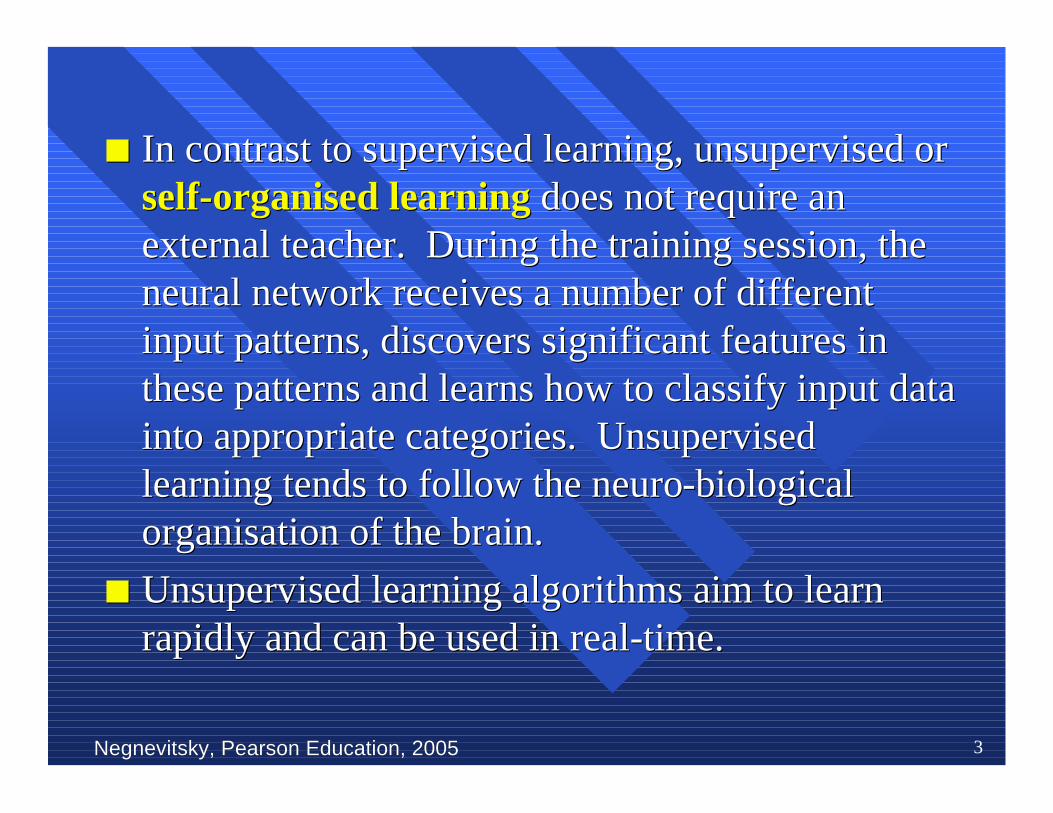
nn In contrast to supervised learning, unsupervised orIn contrast to supervised learning, unsupervised orself-organised learningself-organised learning does not require an does not require anexternal teacher. During the training session, theexternal teacher. During the training session, theneural network receives a number of differentneural network receives a number of differentinput patterns, discovers significant features ininput patterns, discovers significant features inthese patterns and learns how to classify input datathese patterns and learns how to classify input datainto appropriate categories. Unsupervisedinto appropriate categories. Unsupervisedlearning tendslearning tends to follow the to follow the neuro neuro-biological-biologicalorganisation of the brain.organisation of the brain.
nn Unsupervised learning algorithms aim to learnUnsupervised learning algorithms aim to learnrapidly and can be used in real-time.rapidly and can be used in real-time.

Negnevitsky, Pearson Education, 2005Negnevitsky, Pearson Education, 2005 4
InIn 1949, 1949, Donald Hebb proposedDonald Hebb proposed one of the key one of the keyideas in biological learning, commonly known asideas in biological learning, commonly known asHebb’sHebb’s Law Law. . Hebb’sHebb’s Law states that if Law states that if neuron neuron ii is isnear enough to excitenear enough to excite neuron neuron jj and repeatedly and repeatedlyparticipates in its activation, the synaptic connectionparticipates in its activation, the synaptic connectionbetween these twobetween these two neurons neurons is strengthened and is strengthened andneuronneuron jj becomes more sensitive to stimuli from becomes more sensitive to stimuli fromneuronneuron ii..
HebbianHebbian learninglearning
Negnevitsky, Pearson Education, 2005Negnevitsky, Pearson Education, 2005 5
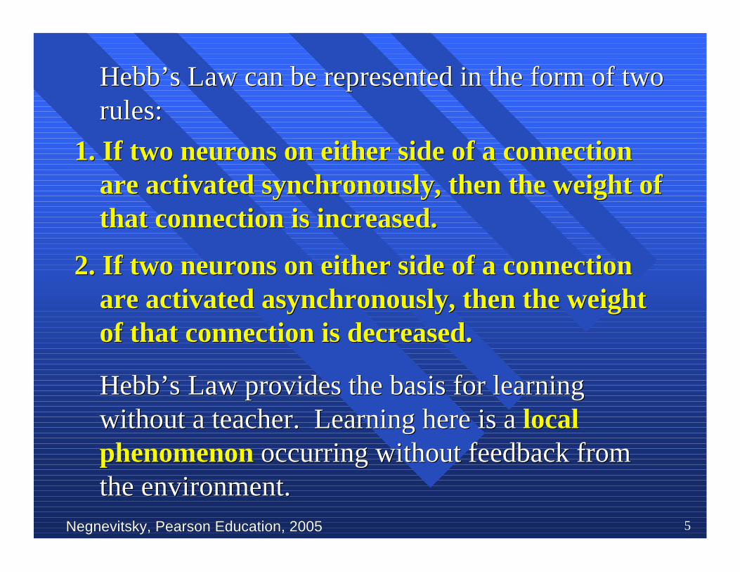
Hebb’s Law can be represented in the form of twoHebb’s Law can be represented in the form of tworules:rules:
1. If two neurons on either side of a connection1. If two neurons on either side of a connectionare activated synchronously, then the weight ofare activated synchronously, then the weight ofthat connection is increased.that connection is increased.
2. If two neurons on either side of a connection2. If two neurons on either side of a connectionare activated asynchronously, then the weightare activated asynchronously, then the weightof that connection is decreased.of that connection is decreased.
Hebb’sHebb’s Law provides the basis for learning Law provides the basis for learningwithout a teacher. Learning here is a without a teacher. Learning here is a locallocalphenomenonphenomenon occurring without feedback from occurring without feedback fromthe environment.the environment.
Negnevitsky, Pearson Education, 2005Negnevitsky, Pearson Education, 2005 6
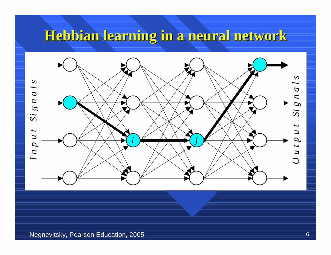
HebbianHebbian learninglearning in a in a neuralneural networknetwork
i j
I n
p u
t S
i g
n a
l s
O u
t p
u t
S i g
n a
l s
Negnevitsky, Pearson Education, 2005Negnevitsky, Pearson Education, 2005 7
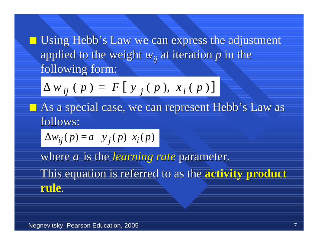
nn UsingUsing Hebb’s Hebb’s Law we can express the adjustment Law we can express the adjustmentapplied to the weightapplied to the weight wwijij at iteration at iteration pp in the in thefollowing form:following form:
nn As a special case, we can represent Hebb’s Law asAs a special case, we can represent Hebb’s Law asfollows:follows:
where where αα is is the the learning ratelearning rate parameter. parameter.
This equation is referred to as the This equation is referred to as the activity productactivity productrulerule..
][ )( ),()( pxpyFpw ijij =∆
)( )( )( pxpypw ijij α=∆
Negnevitsky, Pearson Education, 2005Negnevitsky, Pearson Education, 2005 8
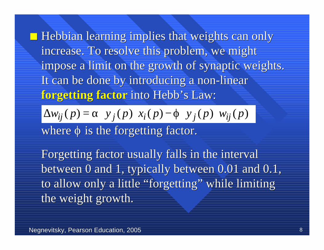
nn HebbianHebbian learning implies that weights can only learning implies that weights can onlyincrease. increase. To resolve this problem, we mightTo resolve this problem, we mightimpose a limit on the growth of synaptic weightsimpose a limit on the growth of synaptic weights..It can be done by introducing a non-linearIt can be done by introducing a non-linearforgetting factorforgetting factor into into Hebb’s Hebb’s Law: Law:
where where ϕϕ is the forgetting factor. is the forgetting factor.
Forgetting factor Forgetting factor usually falls in the intervalusually falls in the intervalbetween 0 and 1, typically betweenbetween 0 and 1, typically between 0.01 and 0.1, 0.01 and 0.1,to allow only a little “forgetting” while limitingto allow only a little “forgetting” while limitingthe weight growth.the weight growth.
)( )( )( )( )( pwpypxpypw ijjijij ϕ−α=∆
Negnevitsky, Pearson Education, 2005Negnevitsky, Pearson Education, 2005 9
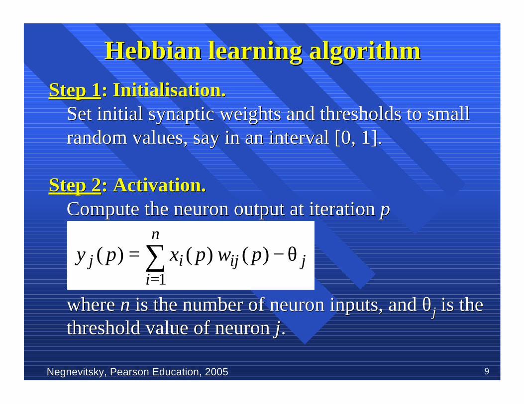
Hebbian learning algorithmHebbian learning algorithm
Step 1Step 1: : InitialisationInitialisation..SetSet initial synaptic weights and thresholds to small initial synaptic weights and thresholds to smallrandom values, say in an interval [0, 1random values, say in an interval [0, 1].].
Step 2Step 2: Activation.: Activation.Compute the neuron output at iteration Compute the neuron output at iteration pp
where where nn is the number of neuron is the number of neuron inputs, and inputs, and θθjj is the is thethreshold value ofthreshold value of neuron neuron jj..
j
n
iijij pwpxpy θ−= ∑
=1
)( )()(
Negnevitsky, Pearson Education, 2005Negnevitsky, Pearson Education, 2005 10
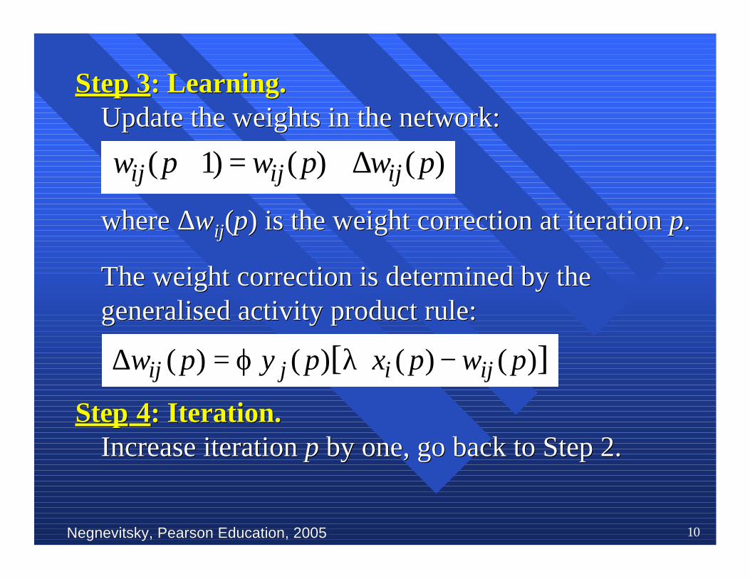
Step 3Step 3:: Learning.Learning.UpdateUpdate the weights in the network: the weights in the network:
wherewhere ∆∆wwijij((pp) is the weight correction at iteration ) is the weight correction at iteration pp..
The weight correction is determined by theThe weight correction is determined by thegeneralised activity product rule:generalised activity product rule:
StepStep 4 4: Iteration.: Iteration.IncreaseIncrease iteration iteration pp by one, go back to Step by one, go back to Step 2.2.
)()()1( pwpwpw ijijij ∆+=+
][ )()()( )( pwpxpypw ijijij −λϕ=∆
Negnevitsky, Pearson Education, 2005Negnevitsky, Pearson Education, 2005 11
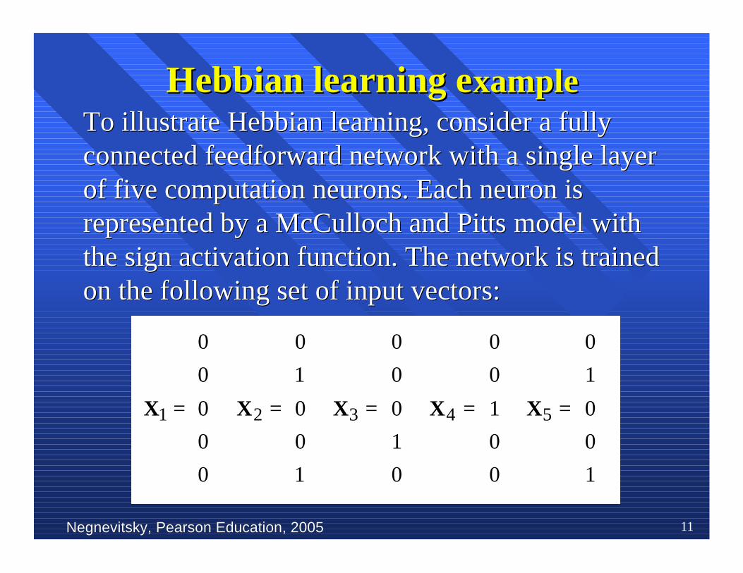
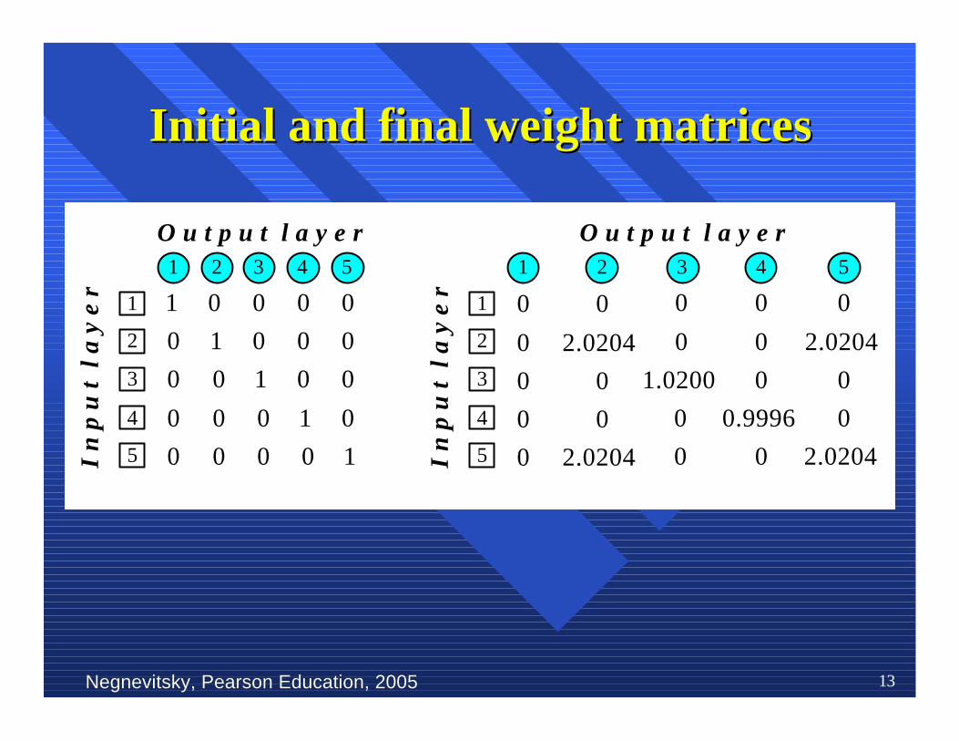
To illustrateTo illustrate Hebbian Hebbian learning, consider a fully learning, consider a fullyconnectedconnected feedforward feedforward network with a single layer network with a single layerof five computation of five computation neuronsneurons. Each . Each neuronneuron is isrepresented by arepresented by a McCulloch McCulloch and and Pitts Pitts model with model withthe sign activation function. The network is trainedthe sign activation function. The network is trainedon the following set of input vectors:on the following set of input vectors:
Hebbian learning eHebbian learning examplexample
=
0
0
0
0
0
1X
=
1
0
0
1
0
2X
=
0
1
0
0
0
3X
=
0
0
1
0
0
4X
=
1
0
0
1
0
5X

Negnevitsky, Pearson Education, 2005Negnevitsky, Pearson Education, 2005 12
Input layer
x1 1
Output layer
2
1 y1
y2x2 2
x3 3
x4 4
x5 5
4
3 y3
y4
5 y5
1
0
0
0
1
1
0
0
0
1
Input layer
x1 1
Output layer
2
1 y1
y2x2 2
x3 3
x4 4
x5
4
3 y3
y4
5 y5
1
0
0
0
1
0
0
1
0
1
2
5
Initial and final states of the networkInitial and final states of the network
Negnevitsky, Pearson Education, 2005Negnevitsky, Pearson Education, 2005 13
O u t p u t l a y e r
I n
p u
t l
a y
e r
1 0 0 0 0
0 1 0 0 0
0 0 1 0 0
0 0 0 1 0
0 0 0 0 1
21 43 5
1
2
3
4
5
O u t p u t l a y e r
I n
p u
t l
a y
e r
0
0
0
0
0
1 2 3 4 5
1
2
3
4
5
0
0
2.0204
0
2.0204
1.0200
0
0
0
0 0.9996
0
0
0
0
0
0
2.0204
0
2.0204
(b).
Initial and final weight matricesInitial and final weight matrices
Negnevitsky, Pearson Education, 2005Negnevitsky, Pearson Education, 2005 14
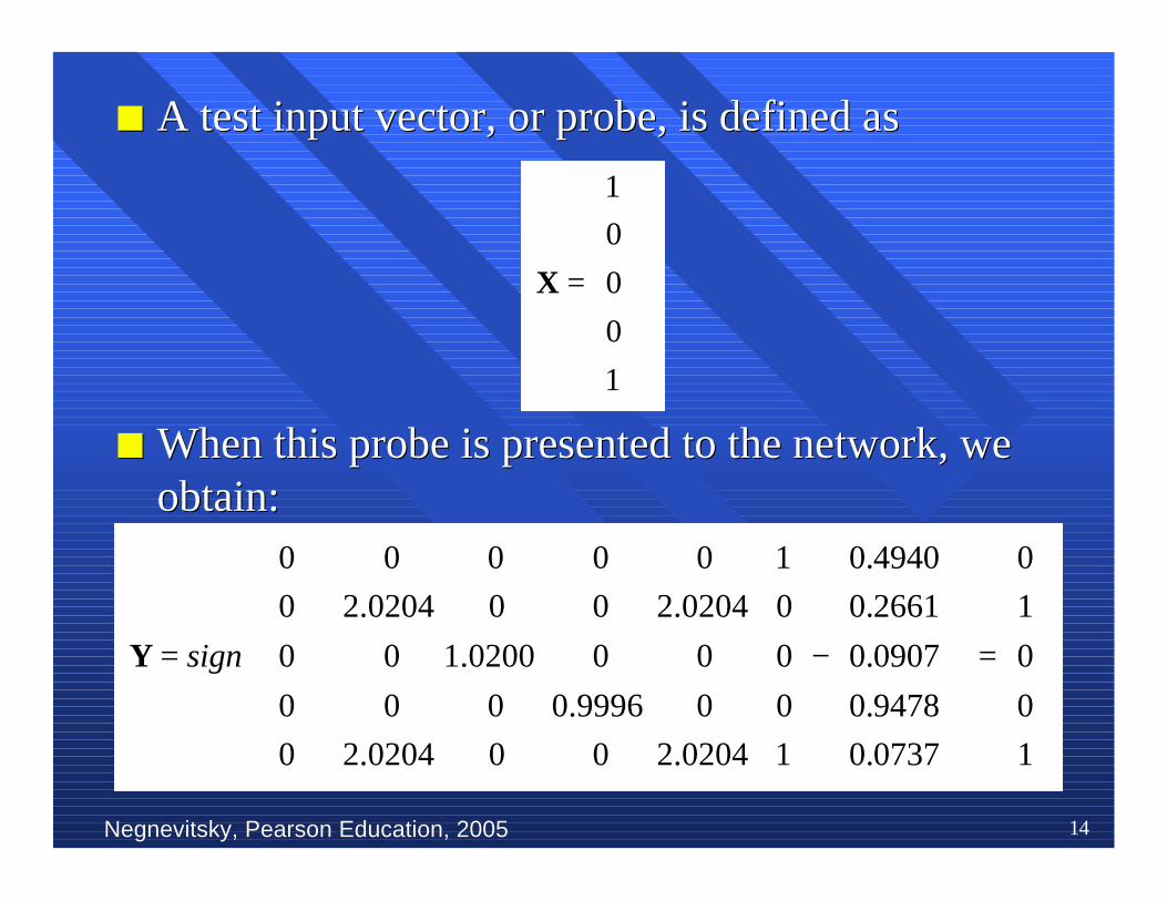
nn When this probe is presented to the network, weWhen this probe is presented to the network, weobtain:obtain:
=
1
0
0
0
1
X
=
−
=
1
0
0
1
0
0737.0
9478.0
0907.0
2661.0
4940.0
1
0
0
0
1
2.0204 0 0 2.0204 0
0 0.9996 0 0 0
0 0 1.0200 0 0
2.0204 0 0 2.0204 0
0 0 0 0 0
signY
nn A test input vector, or probe,A test input vector, or probe, is defined is defined asas
Negnevitsky, Pearson Education, 2005Negnevitsky, Pearson Education, 2005 15
nn InIn competitive learning, competitive learning, neurons neurons compete among compete amongthemselves to be activated.themselves to be activated.
nn WhileWhile in in Hebbian Hebbian learning, several output learning, several output neurons neuronscan be activated simultaneously, in competitivecan be activated simultaneously, in competitivelearning, only a single outputlearning, only a single output neuron neuron is active at is active atany time.any time.
nn TheThe output output neuron neuron that wins the “competition” is that wins the “competition” iscalled the called the winner-takes-allwinner-takes-all neuron neuron..
Competitive Competitive learninglearning
Negnevitsky, Pearson Education, 2005Negnevitsky, Pearson Education, 2005 16
nn The basic idea of competitive learning wasThe basic idea of competitive learning wasintroduced in the early 1970s.introduced in the early 1970s.
nn In the late 1980s, Teuvo Kohonen introduced aIn the late 1980s, Teuvo Kohonen introduced aspecial class of artificial neural networks calledspecial class of artificial neural networks calledself-organising feature mapsself-organising feature maps. These maps are. These maps arebased on competitive learning.based on competitive learning.
Negnevitsky, Pearson Education, 2005Negnevitsky, Pearson Education, 2005 17
OurOur brain is dominated by the cerebral cortex, a brain is dominated by the cerebral cortex, avery complex structure of billions ofvery complex structure of billions of neurons neurons and andhundreds of billions of synapses. The cortexhundreds of billions of synapses. The cortexincludes areas that are responsible for differentincludes areas that are responsible for differenthuman activities (motor, visual, auditory,human activities (motor, visual, auditory,somatosensorysomatosensory, etc.), and , etc.), and associatedassociated with different with differentsensory inputs. We can say that each sensorysensory inputs. We can say that each sensoryinput is mapped into a corresponding area of theinput is mapped into a corresponding area of thecerebral cerebral cortex. cortex. TheThe cortex is a self-organising cortex is a self-organisingcomputational map in the human brain.computational map in the human brain.
What is a self-organisingWhat is a self-organising feature map? feature map?
Negnevitsky, Pearson Education, 2005Negnevitsky, Pearson Education, 2005 18
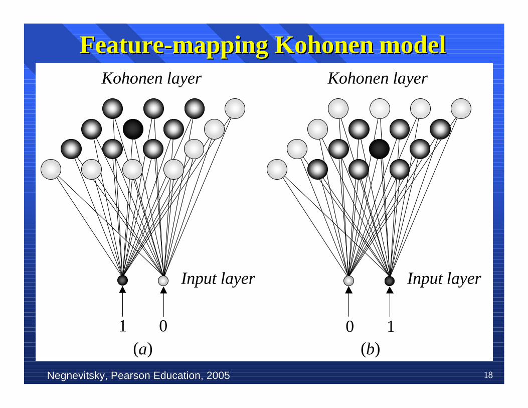
Feature-mappingFeature-mapping Kohonen Kohonen model model
Input layer
Kohonen layer
(a)
Input layer
Kohonen layer
1 0(b)
0 1
Negnevitsky, Pearson Education, 2005Negnevitsky, Pearson Education, 2005 19
nn TheThe Kohonen Kohonen model provides a topological model provides a topologicalmapping.mapping. It places It places a fixed number of input a fixed number of inputpatterns from the input layer into a higher-patterns from the input layer into a higher-dimensional output ordimensional output or Kohonen Kohonen layer. layer.
nn Training in the Kohonen network begins with theTraining in the Kohonen network begins with thewinner’s neighbourhood of a fairly large size.winner’s neighbourhood of a fairly large size.Then, as training proceeds, the neighbourhood sizeThen, as training proceeds, the neighbourhood sizegradually decreases.gradually decreases.
TheThe Kohonen Kohonen networknetwork
Negnevitsky, Pearson Education, 2005Negnevitsky, Pearson Education, 2005 20
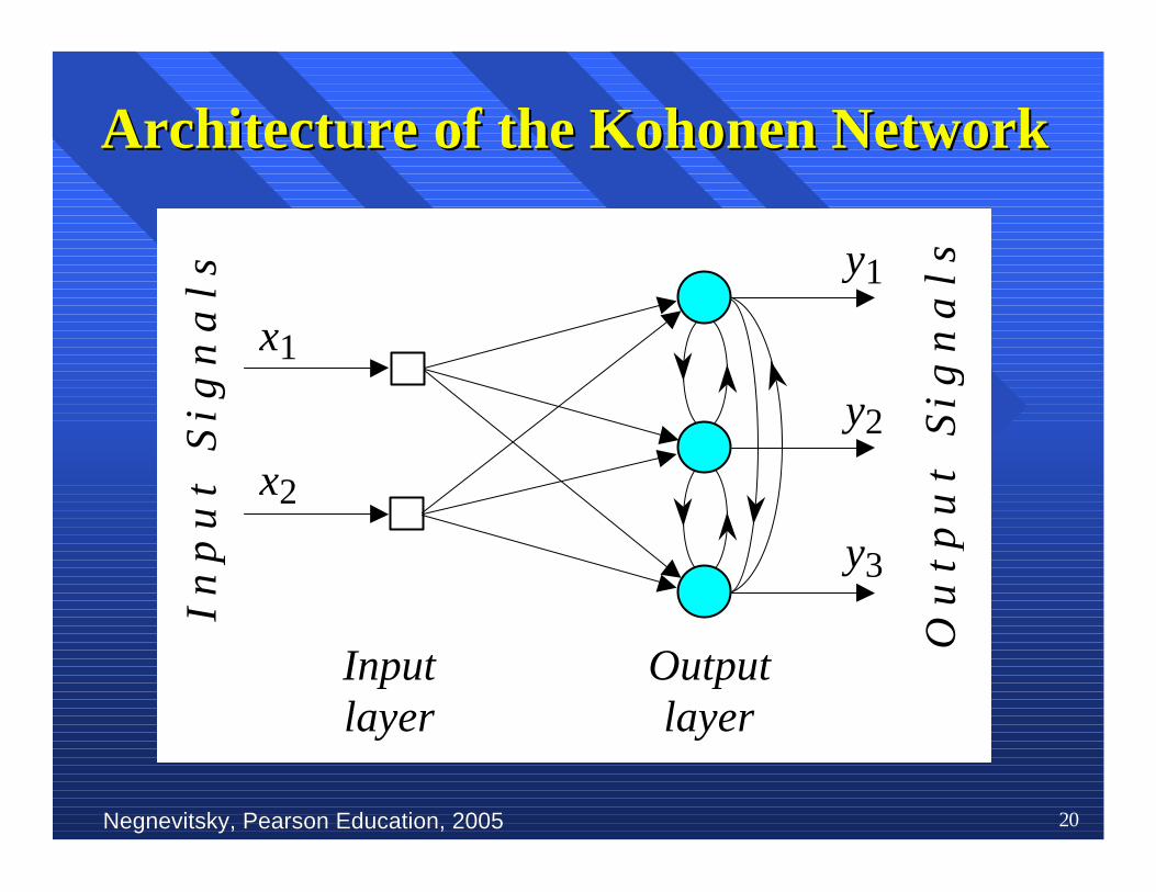
Architecture of the Architecture of the KohonenKohonen Network Network
Inputlayer
O u
t p
u t
S i
g n
a l s
I n
p u
t S
i g
n a
l s
x1
x2
Outputlayer
y1
y2
y3
Negnevitsky, Pearson Education, 2005Negnevitsky, Pearson Education, 2005 21
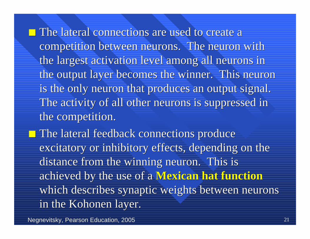
nn The lateral connections are used to create aThe lateral connections are used to create acompetition betweencompetition between neurons neurons. The. The neuron neuron with withthe largest activation level among allthe largest activation level among all neurons neurons in inthe output layer becomes the the output layer becomes the winner. This neuronwinner. This neuronis the only neuronis the only neuron that produces an output signal. that produces an output signal.The activity of all otherThe activity of all other neurons neurons is suppressed in is suppressed inthe competition.the competition.
nn The lateral feedback connections produceThe lateral feedback connections produceexcitatory or inhibitory effects, depending on theexcitatory or inhibitory effects, depending on thedistance from the winning neuron. This isdistance from the winning neuron. This isachieved by the use of a achieved by the use of a Mexican hat functionMexican hat functionwhich describes synaptic weights between neuronswhich describes synaptic weights between neuronsin the Kohonenin the Kohonen layer. layer.

Negnevitsky, Pearson Education, 2005Negnevitsky, Pearson Education, 2005 22
The Mexican hat function of lateral connectionThe Mexican hat function of lateral connection
Connectionstrength
Distance
Excitatoryeffect
Inhibitoryeffect
Inhibitoryeffect
0
1
Negnevitsky, Pearson Education, 2005Negnevitsky, Pearson Education, 2005 23
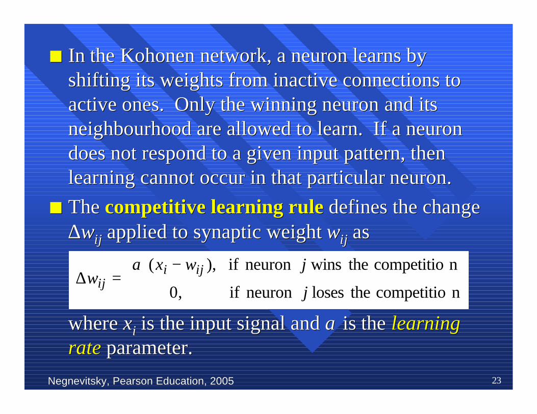
nn In the In the KohonenKohonen network, a network, a neuron neuron learns by learns byshifting its weights from inactive connections toshifting its weights from inactive connections toactive ones. Only the winningactive ones. Only the winning neuron neuron and its and itsneighbourhood are allowed to learn. If aneighbourhood are allowed to learn. If a neuron neurondoes not respond to a given input pattern, thendoes not respond to a given input pattern, thenlearning cannot occur in that particularlearning cannot occur in that particular neuron neuron..
nn The The competitive learning rulecompetitive learning rule defines the change defines the change∆∆wwijij applied to synaptic weight applied to synaptic weight wwijij as as
where where xxii is the input signal and is the input signal and αα is the is the learninglearningraterate parameter. parameter.
−
=∆ncompetitio theloses neuron if ,0
ncompetitio the winsneuron if ),(
j
jwxw iji
ijα
Negnevitsky, Pearson Education, 2005Negnevitsky, Pearson Education, 2005 24
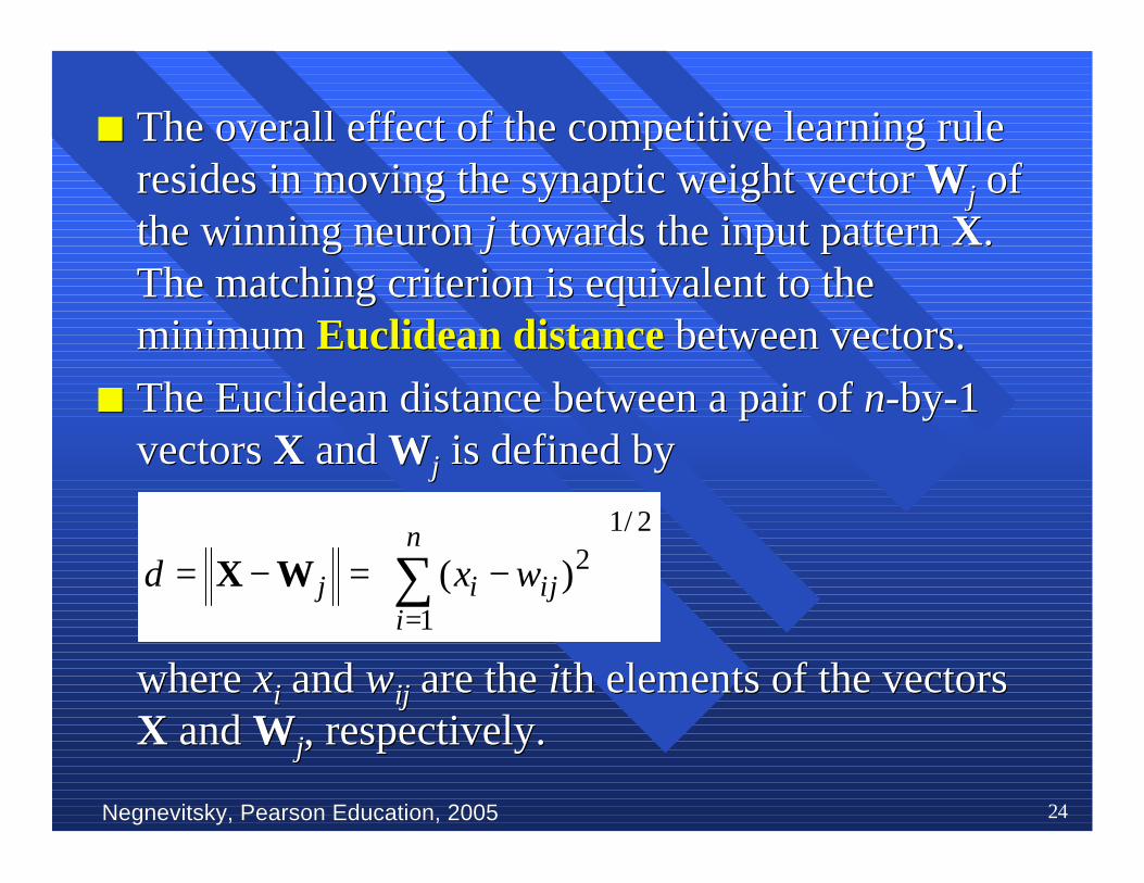
nn The overall effect of the competitive learning ruleThe overall effect of the competitive learning ruleresides in moving the synaptic weight vector resides in moving the synaptic weight vector WWjj of ofthe winningthe winning neuron neuron jj towards the input pattern towards the input pattern XX..The matching criterion is equivalent to theThe matching criterion is equivalent to theminimum minimum Euclidean distanceEuclidean distance between vectors. between vectors.
nn The Euclidean distance between a pair of The Euclidean distance between a pair of nn-by-1-by-1vectors vectors XX and and WWjj is defined by is defined by
wherewhere xxii and and wwijij are the are the iithth elements of the vectors elements of the vectorsXX and and WWjj,, respectively. respectively.
2/1
1
2)(
−=−= ∑
=
n
iijij wxd WX
Negnevitsky, Pearson Education, 2005Negnevitsky, Pearson Education, 2005 25
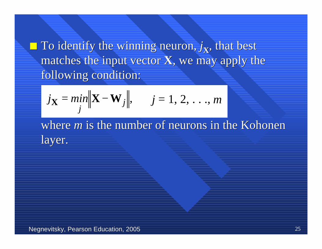
nn To identify the winningTo identify the winning neuron neuron,, jjXX, that best, that bestmatches the input vector matches the input vector XX, we may apply the, we may apply thefollowing condition:following condition:
where where mm is the number of is the number of neurons neurons in the in the Kohonen Kohonenlayer.layer.
,jj
minj WXX −= j = 1, 2, . . ., m
Negnevitsky, Pearson Education, 2005Negnevitsky, Pearson Education, 2005 26
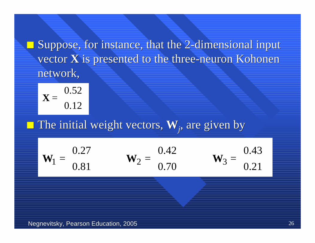
nn Suppose, for instance, that the 2-dimensional inputSuppose, for instance, that the 2-dimensional inputvector vector XX is presented to the three-neuron Kohonen is presented to the three-neuron Kohonennetwork,network,
nn The initial weight vectors, The initial weight vectors, WWjj, are given by, are given by
=
12.0
52.0X
=
81.0
27.01W
=
70.0
42.02W
=
21.0
43.03W
Negnevitsky, Pearson Education, 2005Negnevitsky, Pearson Education, 2005 27
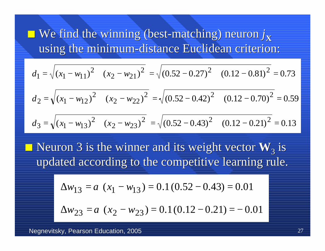
nn We find the winning (best-matching)We find the winning (best-matching) neuron neuron jjXX
using the minimum-distance Euclidean criterionusing the minimum-distance Euclidean criterion::
2212
21111 )()( wxwxd −+−= 73.0)81.012.0()27.052.0( 22 =−+−=
2222
21212 )()( wxwxd −+−= 59.0)70.012.0()42.052.0( 22 =−+−=
2232
21313 )()( wxwxd −+−= 13.0)21.012.0()43.052.0( 22 =−+−=
nn Neuron 3 is the winner and its weight vector Neuron 3 is the winner and its weight vector WW33 is isupdated according to the competitive learningupdated according to the competitive learning rule. rule.
0.01 )43.052.0( 1.0)( 13113 =−=−=∆ wxw α
0.01 )21.012.0( 1.0)( 23223 −=−=−=∆ wxw α
Negnevitsky, Pearson Education, 2005Negnevitsky, Pearson Education, 2005 28
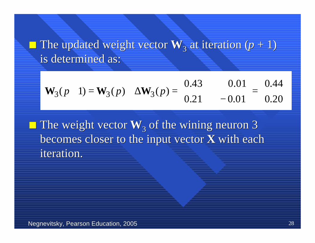
nn The updated weight vector The updated weight vector WW33 at iteration ( at iteration (pp + 1) + 1)is determined as:is determined as:
nn The weight vector The weight vector WW33 of the wining of the wining neuron neuron 3 3becomes closer to the input vector becomes closer to the input vector XX with each with eachiteration.iteration.
=
−
+
=∆+=+
20.0
44.0
01.0
0.01
21.0
43.0)()()1( 333 ppp WWW
Negnevitsky, Pearson Education, 2005Negnevitsky, Pearson Education, 2005 29
Step 1Step 1:: InitialisationInitialisation..
Set initial synaptic weights to small random Set initial synaptic weights to small randomvalues, say in an interval [0, 1], and assign a smallvalues, say in an interval [0, 1], and assign a smallpositive value to the learning rate parameter positive value to the learning rate parameter αα..
Competitive Learning AlgorithmCompetitive Learning Algorithm

Negnevitsky, Pearson Education, 2005Negnevitsky, Pearson Education, 2005 30
Step 2Step 2:: Activation and Similarity MatchingActivation and Similarity Matching..
Activate the Kohonen network by applying theActivate the Kohonen network by applying theinput vector input vector XX, and find the winner-takes-all (best, and find the winner-takes-all (bestmatching) neuron matching) neuron jjXX at iteration at iteration pp, using the, using theminimum-distance Euclidean criterionminimum-distance Euclidean criterion
where where nn is the number of is the number of neurons neurons in the input in the inputlayer, and layer, and mm is the number of is the number of neurons neurons in in thetheKohonen layer.Kohonen layer.
,)()()(
2/1
1
2][
−=−= ∑=
n
iijij
jpwxpminpj WXX
j = 1, 2, . . ., m
Negnevitsky, Pearson Education, 2005Negnevitsky, Pearson Education, 2005 31
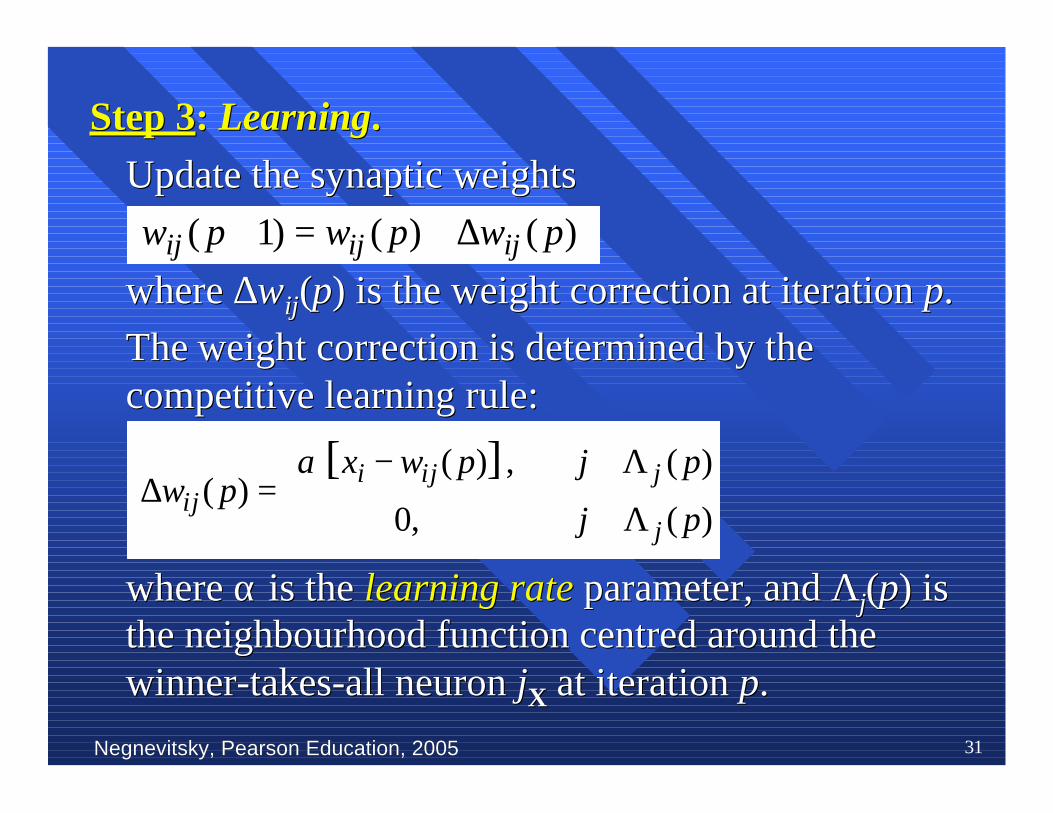
Step 3Step 3:: LearningLearning..
UpdateUpdate the synaptic weights the synaptic weights
where where ∆∆wwijij((pp) is the weight correction at iteration ) is the weight correction at iteration pp..
TheThe weight correction is determined by the weight correction is determined by thecompetitive learning rule:competitive learning rule:
where where αα is the is the learning ratelearning rate parameter, and parameter, and ΛΛjj((pp) is) isthe neighbourhood function centred around thethe neighbourhood function centred around thewinner-takes-allwinner-takes-all neuron neuron jjXX at iteration at iteration pp..
)()()1( pwpwpw ijijij ∆+=+
Λ∉
Λ∈−=∆
)( ,0
)( , )( )(
][pj
pjpwxpw
j
jijiij
α
Negnevitsky, Pearson Education, 2005Negnevitsky, Pearson Education, 2005 32
Step 4Step 4:: IterationIteration..
Increase iteration Increase iteration pp by one, go back to Step 2 and by one, go back to Step 2 andcontinue until the minimum-distance Euclideancontinue until the minimum-distance Euclideancriterion is satisfied, or no noticeable changescriterion is satisfied, or no noticeable changesoccur in the feature map.occur in the feature map.
Negnevitsky, Pearson Education, 2005Negnevitsky, Pearson Education, 2005 33
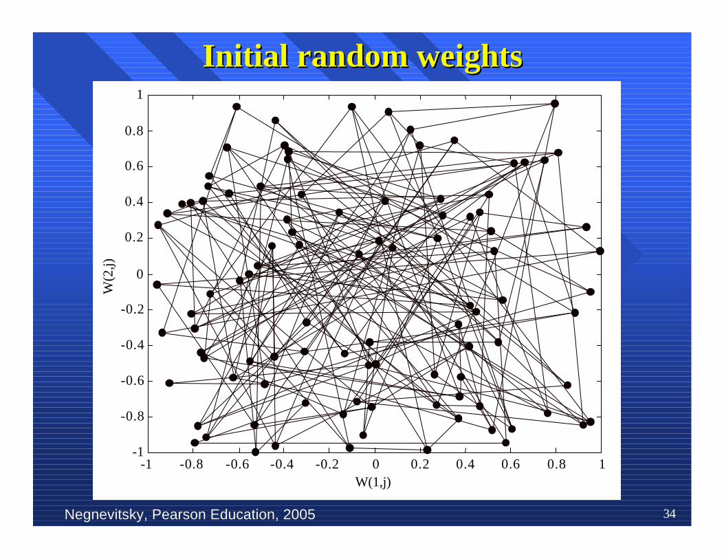
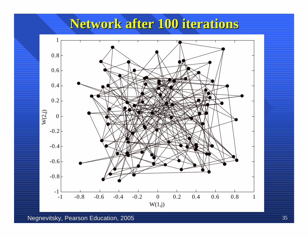
nn To illustrate competitive learning, consider theTo illustrate competitive learning, consider theKohonenKohonen network with 100 network with 100 neurons neurons arranged in the arranged in theform of a two-dimensional lattice with 10 rows andform of a two-dimensional lattice with 10 rows and10 columns. The network is required to classify10 columns. The network is required to classifytwo-dimensional input two-dimensional input vectors vectors −− each neuron in the each neuron in thenetwork should respond only to the input vectorsnetwork should respond only to the input vectorsoccurring in its region.occurring in its region.
nn The network is trained with 1000 two-dimensionalThe network is trained with 1000 two-dimensionalinput vectors generated randomly in a squareinput vectors generated randomly in a squareregion in the interval between –1 and +1. region in the interval between –1 and +1. TheThelearning rate parameter learning rate parameter αα is equal to 0.1. is equal to 0.1.
Competitive learning in theCompetitive learning in the Kohonen Kohonen network network
Negnevitsky, Pearson Education, 2005Negnevitsky, Pearson Education, 2005 34
-0.8 -0.6 -0.4 -0.2 0 0.2 0.4 0.6 0.8 1W(1,j)
-1-1
-0.8
-0.6
-0.4
-0.2
0
0.2
0.4
0.6
0.8
1W
(2,j)
Initial random weightsInitial random weights
Negnevitsky, Pearson Education, 2005Negnevitsky, Pearson Education, 2005 35
Network after 100 iterationsNetwork after 100 iterations
-0.8 -0.6 -0.4 -0.2 0 0.2 0.4 0.6 0.8 1W(1,j)
-1-1
-0.8
-0.6
-0.4
-0.2
0
0.2
0.4
0.6
0.8
1W
(2,j)
Negnevitsky, Pearson Education, 2005Negnevitsky, Pearson Education, 2005 36
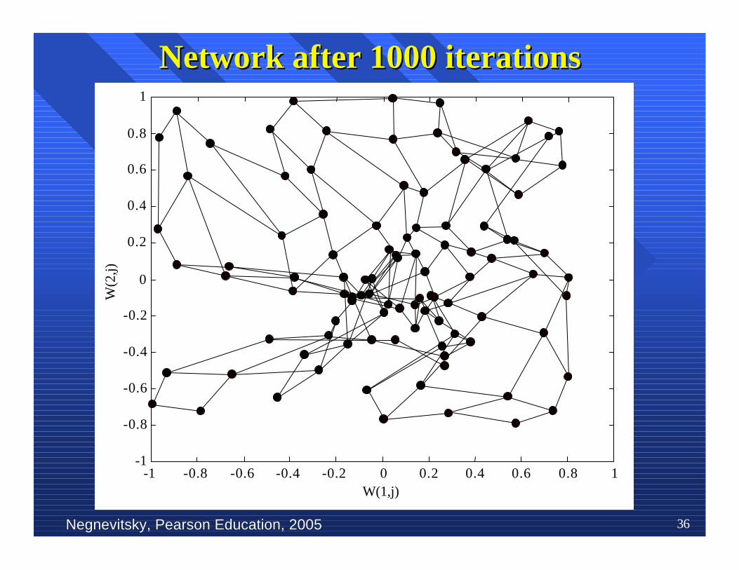
Network after 1000 iterationsNetwork after 1000 iterations
-0.8 -0.6 -0.4 -0.2 0 0.2 0.4 0.6 0.8 1W(1,j)
-1-1
-0.8
-0.6
-0.4
-0.2
0
0.2
0.4
0.6
0.8
1W
(2,j)
Negnevitsky, Pearson Education, 2005Negnevitsky, Pearson Education, 2005 37
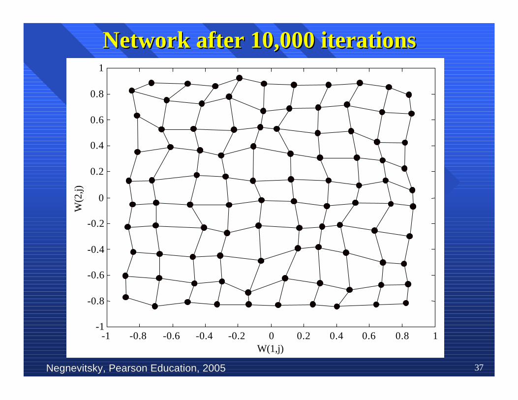
Network after 10,000 iterationsNetwork after 10,000 iterations
-0.8 -0.6 -0.4 -0.2 0 0.2 0.4 0.6 0.8 1W(1,j)
-1-1
-0.8
-0.6
-0.4
-0.2
0
0.2
0.4
0.6
0.8
1W
(2,j)