Artificial neural networks for loudspeaker modelling and fault ...
Upload
khangminh22Category
view
1download
0
This project has received funding from the
European Union’s PRIMA research and
innovation programme
KARMA Karst Aquifer Resources availability and quality in the Mediterranean Area
Application of Artificial Neural Network models at KARMA test sites Deliverable 4.3
Authors:
Andreas Wunsch (KIT), Tanja Liesch (KIT), Nico Goldscheider (KIT), Emna
Gargouri-Ellouze (ENIT), Tegawende Arnaud Ouedraogo (ENIT), Fairouz Slama
(ENIT), Rachida Bouhlila (ENIT), Guillaume Cinkus (UM), Naomi Mazzilli (UM),
Hervé Jourde (UM)
Date: August 2021

2 Application of Artificial Neural Network models
Technical References
Project Acronym KARMA
EU Program, Call and Topic PRIMA, Multi-topic 2018, Water resources availability and quality within catchments and aquifers
Project Title Karst Aquifer Resources availability and quality in the Mediterranean Area
Project Coordinator Prof. Dr. Nico Goldscheider, Karlsruhe Institute of Technology (KIT), [email protected]
Project Duration September 2019 - August 2022
Deliverable No., Name D4.3, Application of artificial neural network models at the KARMA test sites
Dissemination Level* PU
Work Package WP4: Modeling Tools
Task Task 4.2 Development of lumped-parameter and artificial neural network models
Lead beneficiary Karlsruhe Institute of Technology (KIT)
Contributing beneficiary/ies Bundesanstalt für Geowissenschaften und Rohstoffe (BGR), University of Malaga (UMA), University of Montpellier (UM), Sapienza University of Rome (URO), Ecole nationale d’Ingenieurs de Tunis (ENIT), American University of Beirut (AUB)
Due Date August 2021
Actual Submission Date
* PU = public
CO = Confidential, only for members of the consortium (including the Commission Services)
RE = Restricted to a group specified by the consortium (including the Commission Services)
Version History
Version Date
1.0 July 2021
2.0 August 2021

3 Application of Artificial Neural Network models
Project Partners
(Coordinator)
Participant No *
Organization Country
1 (Coordinator) Karlsruhe Institute of Technology (KIT) Germany
2 Partner 1 Federal Institute for Geosciences and Natural Resources (BGR)
Germany
3 Partner 2 University of Malaga (UMA) Spain
4 Partner 3 University of Montpellier (UM) France
5 Partner 4 University of Rome (URO) Italy
6 Partner 5 American University of Beirut (AUB) Lebanon
7 Partner 6 Ecole National d’Ingénieurs de Tunis (ENIT)
Tunisia

4 Application of Artificial Neural Network models
Executive Summary
Work package 4 of the KARMA project focuses on the development and comparison of transferable
modelling tools for improved predictions concerning the impacts of climate change, floods, droughts
and land-use changes on karst aquifers. In this context, the application of Artificial Neural Networks to
model karst spring discharge time series is demonstrated in deliverable 4.3. Modeling results from six
different test sites are shown by using an approach based on 1D-Convolutional Neural Networks, which
have been shown to be fast and reliable for strongly related tasks such as groundwater level
predictions. Using this approach, even for complex systems, highly accurate results can be achieved
with comparably little time effort and only little prior knowledge about the system being necessary.
However, no deeper knowledge of the system can be derived from the model and in areas where too
few data are available, no satisfying results can be achieved.
Accompanying model codes will be published as part of deliverable 4.4.

5 Application of Artificial Neural Network models
1 Table of Content
Technical References ..........................................................................................................................2
Version History ...................................................................................................................................2
Project Partners ..................................................................................................................................3
Executive Summary.............................................................................................................................4
2 Introduction ................................................................................................................................6
3 Material and Methods.................................................................................................................7
3.1 Available Data .....................................................................................................................7
3.2 Available Data and Preprocessing - Zaghouan Site ...............................................................8
3.3 Convolutional Neural Networks ......................................................................................... 11
3.4 Model Calibration and Evaluation ...................................................................................... 11
3.5 Alternative Approach – Zaghouan Site ............................................................................... 12
3.5.1 ANN Models .............................................................................................................. 12
3.5.2 Simulation and Evaluation Approach .......................................................................... 13
4 Results and Discussion .............................................................................................................. 14
4.1 Aubach Spring (Austria) ..................................................................................................... 14
4.2 Lez Spring (France) ............................................................................................................ 15
4.3 Unica Springs (Slovenia) ..................................................................................................... 15
4.4 Gato Cave Spring (Spain).................................................................................................... 16
4.5 Qachqouch Spring (Lebanon) ............................................................................................. 17
4.6 Nymphea Spring (Tunisia) .................................................................................................. 18
4.6.1 MLP ........................................................................................................................... 18
4.6.2 CNN ........................................................................................................................... 19
4.6.3 LSTM.......................................................................................................................... 20
4.7 Comparison with lumped parameter model results ........................................................... 21
5 Conclusions ............................................................................................................................... 22
References ........................................................................................................................................ 22
6 Application of Artificial Neural Network models
2 Introduction Modeling Karst water resources is challenging, because water flow is highly variable due to the
unknown conduit networks. Therefore a large variety of different modeling approaches exists (Jeannin
et al., 2021), most of them requiring a certain level of background knowledge about the system in
order to achieve high quality results. In contrary, deep learning approaches can be applied without
detailed system knowledge necessary, by being able to establish a relationship between relevant
forcings, such as climatic inputs, and outputs, i.e. spring discharge, on their own. To date, Artificial
Neural Networks (ANN) remain an exotic tool in the karst modeling community. Nevertheless, different
types of ANNs have been applied in modeling karst water resources for quite a long time, with the
study of Johannet et al. (1994) being even one of the first applications of ANNs in water related
research. In the context of the KARMA project mainly Convolutional Neural Networks (CNN) are
applied to model karst spring discharge at several sites. CNNs have been shown to be fast and reliable
for the closely related application of groundwater level forecasting (Wunsch et al., 2021) and also have
been rudimentarily applied to Karst spring modeling (Jeannin et al. 2021). According to the study of
Wunsch et al. (2021), CNNs are significantly faster and more stable than other methods such and NARX
(nonlinear autoregressive models with exogenous inputs) and LSTM (long short-term memory
networks), and usually show similar or better accuracy in predicting groundwater levels, which makes
them the preferable approach for modeling karst spring discharge. Even though such data driven
approaches rely on a comparably large data basis and do usually not enhance system knowledge such
as lumped parameter models can do, they are a powerful tool to achieve high quality simulations in a
relatively short time.
All KARMA test sites were scanned for a suitable data basis to apply ANN modeling. Because of the fact
that gapless and as long as possible time series of both spring discharge (target variable) and climatic
inputs (i.e. precipitation, temperature, etc.) have to be available, the Eastern Ronda Mountains test
site in Spain and the Gran Sasso test site in Italy were not suitable for ANN application. A large number
of data gaps and too short time series prevented ANN application in these two areas. The Zaghouan
site in Tunisia holds a somewhat unique position in this respect. On the one hand, the data are very
old and had to be digitized first, on the other hand, a certain effort was made to generate input data
and thus build models, while the other sites were modeled with current and already existing
meteorological series. The modeling here was done exclusively by the local partner ENIT and therefore
includes some further analysis and a brief comparison of CNNs with two other types of models, namely
Multi-Layer Perceptron (MLP) and Long Short-term Memory (LSTM) models. For these reasons the
Zaghouan site is presented in separate sub topics in this report.
To compensate for the two unusable test sites in Spain and Italy, additional alternative karst
areas/springs were used for ANN modeling, so that results from a total of six karst springs can be
presented: Aubach spring (Hochifen-Gottesacker karst area) in Austria, Lez spring in France, Unica
springs in Slovenia, Gato cave spring in Spain, Qachqouch spring in Lebanon and Nymphea spring
(Zaghouan area) in Tunisia (Figure 1). For descriptions of the study areas we refer to Deliverable 4.2.
In this report we will focus on description of data, models and results.

7 Application of Artificial Neural Network models
Figure 1: Location of the karst springs modeled with ANNs and carbonate outcrops after WOKAM (Chen et al., 2017a)
3 Material and Methods
3.1 Available Data Very different data were available for each site especially in terms of climatic parameters, temporal
resolution and available period. Table 1 gives a summary of the used data for each site. Sometimes
more parameters, additional climate stations, other periods or even other temporal resolutions were
available and have been tested. The used data represents a compromise of longest available time
period, as large as possible number of relevant parameters, and model performance.
Table 1: Data basis overview of all five modeled sites.
Spring Period Temporal Resolution
Input Parameters
Aubach 2012-2020 Hourly Precipitation, temperature and snow routine output for climate stations Walmendinger Horn, Diedamskopf and Oberstdorf. Additional Parameter: Tsin
Lez 2008-2019 Daily Precipitation (interpolated), Prades-le-Lez climate station: temperature
Unica 1961-2018 Daily Postojna climate station: precipitation, pot. evaporation, temperature, rel. humidity, snow, new snow; Cerknica climate station: precipitation, snow, new snow
Gato Cave 1970-2015 Daily Precipitation, temperature
Qachqouch 2015-2020 Daily Climate station 1 (950m): temperature, rel. humidity; climate station 2 (1750m): temperature, precipitation, evapotranspiration
In case of Aubach spring the discharge is significantly influenced by seasonal snow accumulation and
melting (Chen et al., 2017b) and no directly measured data about snowfall or snowmelt were available.
Therefore a snowmelt routine is run as preprocessing of the meteorological input data as described in
8 Application of Artificial Neural Network models
Chen et al. (2018). This routine is a slightly modified version (after Hock 1999) of the HBV hydrological
model snow routine (e.g. Bergström 1975, 1995; Seibert 2000; Kollat et al. 2012), which redistributes
the precipitation time series in accordance with probable snow accumulation and snowmelt and
produces an additional input parameter for each climate station. Such parameter can potentially
replace the original precipitation input; however, the performance of the model was better when
including both the original and the redistributed precipitation. Other test sites either had snow data
from climate stations available (e.g. Unica) or are not (significantly) influenced by snow accumulation
and snowmelt (e.g. Lez). This is also shown in Deliverable 4.2, were a precipitation redistribution using
this snow routine for all sites is performed and significant redistribution can be observed only for
Aubach and Unica.
In some cases, ANN models can profit from artificial input data that provides information on the season
and therefore the current position in the annual cycle. Therefore, the influence of a sinus signal input
fitted to the temperature curve (Tsin), which is known from experience to often improve modeling
results, is tested. For one of the five sites (Aubach spring) such input provided improved performance
and was therefore also used.
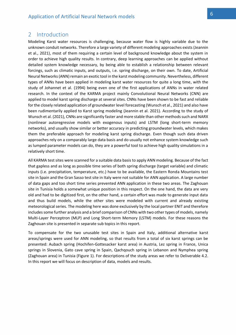
3.2 Available Data and Preprocessing - Zaghouan Site In our ANN modelling approach, the data used are: the meteorological input data or exogenous data
to the karst and the output data (discharge) or endogenous data. The input data considered are
rainfall, mean temperature and pressure on a daily scale. The rainfall data considered are those of the
"Zaghouan controle" station (latitude: 36.39583; longitude: 10.14917) which extend from 1915 to
1944. However, there are gaps in the data for the entire year of 1929 and January 1930. These gaps
were filled by a linear interpolation using data from the nearby station "Zaghouan SM" (latitude:
36.40306; longitude: 10.14472) (Figure 2).
Figure 2: Location of study rainfall stations
This data treatment allows us to obtain the entire series of daily and weekly cumulative rainfall (Figure
3 and Figure 4).

9 Application of Artificial Neural Network models
Figure 3: Daily rainfall from 1915 to 1944 at Zaghouan contrôle station
Figure 4: Cumulative weekly rainfall from 1915 to 1944 at Zaghouan contrôle station
A statistical description of the weekly rainfall series gives us the following table (Table 2). It can be seen
that the first quartile for weekly series is equal to 0 mm, which is explained by the low number of rainy
days, 77 days per year (this is most noticeable for the daily series). Indeed, Zaghouan is located in a
semi-arid zone. In addition to the rainfall data used as input, we used a synthetic daily and weekly
series of median temperature and pressure values, as data from 1915 to 1943 are not available at the
moment. This synthetic series was built up from temperature and pressure data from 1943 to 2008
from the Oued El Kebir dam. Figure 5 shows the different percentiles on a weekly and daily scale.
Subsequently, we considered the median and repeated it several times to obtain our weekly and daily
temperature and pressure series.
10 Application of Artificial Neural Network models
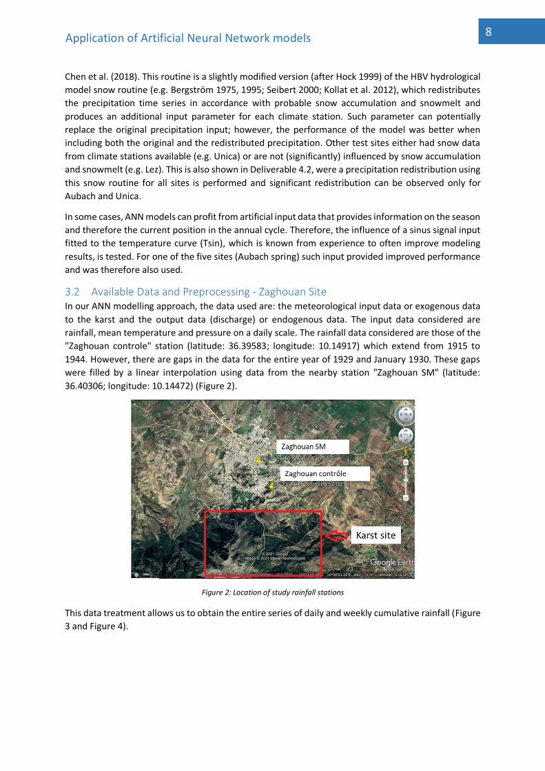
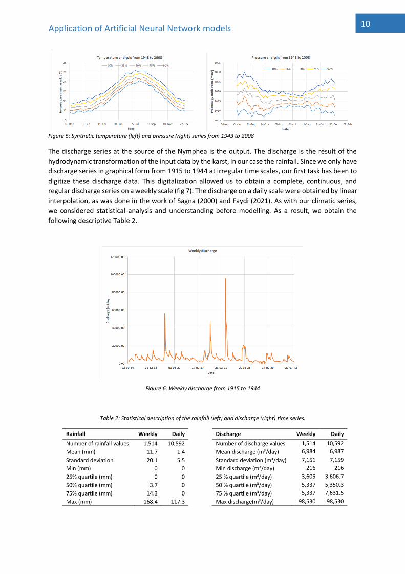
Figure 5: Synthetic temperature (left) and pressure (right) series from 1943 to 2008
The discharge series at the source of the Nymphea is the output. The discharge is the result of the
hydrodynamic transformation of the input data by the karst, in our case the rainfall. Since we only have
discharge series in graphical form from 1915 to 1944 at irregular time scales, our first task has been to
digitize these discharge data. This digitalization allowed us to obtain a complete, continuous, and
regular discharge series on a weekly scale (fig 7). The discharge on a daily scale were obtained by linear
interpolation, as was done in the work of Sagna (2000) and Faydi (2021). As with our climatic series,
we considered statistical analysis and understanding before modelling. As a result, we obtain the
following descriptive Table 2.
Figure 6: Weekly discharge from 1915 to 1944
Table 2: Statistical description of the rainfall (left) and discharge (right) time series.
Rainfall Weekly Daily
Number of rainfall values 1,514 10,592 Mean (mm) 11.7 1.4 Standard deviation 20.1 5.5 Min (mm) 0 0 25% quartile (mm) 0 0 50% quartile (mm) 3.7 0 75% quartile (mm) 14.3 0 Max (mm) 168.4 117.3
Discharge Weekly Daily
Number of discharge values 1,514 10,592
Mean discharge (m³/day) 6,984 6,987
Standard deviation (m³/day) 7,151 7,159
Min discharge (m³/day) 216 216
25 % quartile (m³/day) 3,605 3,606.7
50 % quartile (m³/day) 5,337 5,350.3
75 % quartile (m³/day) 5,337 7,631.5
Max discharge(m³/day) 98,530 98,530

11 Application of Artificial Neural Network models
3.3 Convolutional Neural Networks Convolutional Neural Networks (LeCun et al., 2015) are a common tool in object recognition, image
classification and signal processing. The general structure usually uses sequences of blocks, consisting
of several layers, which are typically at least one convolutional layer and a pooling layer. The dimension
of the data predefines the dimension of the convolutional layers (1D in case of time series) that use
filters with a fixed size (kernel size, receptive field) to produce a certain number of feature maps of the
input data. Often a larger number of filters is used, each of them recognizing different input data
characteristics (features). Afterwards downsampling and therefore information consolidation is
performed in a pooling layer. A wide range of model structures based on these blocks are possible.
Usually additional layers to prevent, for example, exploding gradients (e.g. using batch normalization
layers) or overfitting of the model (e.g. using dropout layers) are also used within such block
sequences. Often long short-term memory networks are preferred over 1D-CNNs because they are by
definition not prone to the vanishing gradient problem, nevertheless we have shown in earlier studies
(Wunsch et al., 2021) that for groundwater modeling 1D-CNNs are superior because they are faster,
often show higher performance and furthermore produce reliably stable results.
We use an ensemble of 10 models to reduce the dependency of the model on the random initialization
of the layer weights and calculate 100 forecasts for each of these 10 models based on a Monte-Carlo
dropout approach, which are used to derive the 95%-model uncertainty interval. Each of the used
CNN models follows the general design shown in Figure 7. Hyperparameters are derived as described
in the following section. Python 3.8 (van Rossum, 1995) and the following frameworks and libraries are
used to implement all models: TensorFlow and its Keras API (Abadi et al., 2015; Chollet, 2015), Numpy
(van der Walt et al., 2011), Pandas (McKinney, 2010; Reback et al., 2020), Scikit-Learn (Pedregosa et
al., 2011), Unumpy (Lebigot, 2010), Matplotlib (Hunter, 2007) and Bayesian Optimization (Nogueira,
2014).
Figure 7: CNN model design used to simulate karst spring discharge
3.4 Model Calibration and Evaluation While training, optimizing and testing the model, data leakage is prevented by splitting the time series
of each site into four parts of which the largest part is used for training, a smaller part for early stopping
to prevent overfitting the model (validation), and two other parts as test set during optimization and
as final test set to evaluate the model performance (Table 3).
Table 3: Time series splitting for each test site for model training, optimization and testing
Training Validation Optimization Testing
Aubach 11/2012-2017 2018 2019 1/2020-10/2020
Lez 10/2008-2015 2016 2017 2018+2019
Unica 1961-08/2012 09/2012-10/2014 11/2014-09/2016 10/2016-2018
Gato Cave 1970-08/2003 09/2003-08/2007 09/2007-08/2011 09/2011-05/2015
Qachqouch 09/2015-09/2018 10/2018-02/2019 02/2019-09/2019 10/2019-01/2020

12 Application of Artificial Neural Network models
Further, Bayesian optimization is used to derive the length of the input sequence (search space is site
dependent), the batch size (24 to 28) during training, the number of filters in the 1D-Conv layer (24 to
28), and the number of neurons in the first dense layer (24 to 28). These hyperparameters are
optimized on model performance in terms of mean squared error (objective function) in the
optimization set. While the kernel size was set to 3 for all of the models, the dropout rate was chosen
site dependently (as high as possible with meaningful results, at least 10%), as well as the number of
training epochs, the early stopping patience and the number of Bayesian optimization steps (Table
4). We mostly perform at least 50 optimization steps and stop either when 80 steps are reached or
after no improvement for 10 steps (Stop Criteria).
Table 4: Manually chosen Hyperparameters.
Dropout
Rate
Training
Epochs
Early Stopping
Patience
Bayesian Optimization Steps
(Min/Max/Stop Criteria)
Aubach 10% 200 20 50/80/10
Lez 50% 200 15 25/50/10
Unica 10% 100 10 50/80/10
Gato Cave 50% 100 10 50/80/10
Qachqouch 10% 500 20 50/80/10
To evaluate the performance of the models, several metrics are calculated: Nash-Sutcliffe Efficiency
(NSE) (Nash and Sutcliffe, 1970), squared Pearson r (R²), root mean squared error (RMSE), Bias (Bias)
as well as Kling-Gupta-Efficiency (KGE) (Gupta et al., 2009). For squared Pearson r the notation of the
coefficient of determination (R²) is used, because the linear fit between simulated and observed
discharge, thus of a simple linear model is compared, which makes them equal in this case. Further,
individual performance on high, medium and low flow were investigated using mainly RMSE and Bias.
Especially, NSE and KGE seem rather unintuitive for such evaluation, because the reference values for
calculation change, which makes comparison and interpretation difficult. The thresholds to distinguish
between high/medium and medium/low flow are defined as the 90% quantile of Q and 40% of the
mean Q value, respectively.
3.5 Alternative Approach – Zaghouan Site
3.5.1 ANN Models In a comparative modelling approach, we considered three types of ANN models: Multi-layer
perceptron (MLP), Long Short-Term Memory (LSTM) and Convolutional Neural Network (CNN). In
addition, in order to characterize the most suitable time scale for our system, we performed daily and
weekly simulations for each model. For each temporal approach, a simulation configuration has been
adopted: it consists in predicting a single future value of flow knowing only the data on rainfall, average
temperature and pressure of the previous days. This configuration is called "seq2val forecasting" or
"one-step ahead forecasting". In order to prevent overfitting, we used the "dropout" regularization
method which consists in randomly disactivating some neurons at each iteration.
The MLP model is a model consisting of interconnected neurons. It has hidden layers of Nc neurons
each and a linear output layer consisting of one neuron(Kong-A-Siou et al., 2015). Our MLP model
consists of two hidden layer and one linear output neuron.

13 Application of Artificial Neural Network models
The LSTM model is a recurrent neural network model. It uses stochastic approximation through
sequential time series. It consists of several cells; each cell comprising the input gate, the output gate
and the forget gate. The LSTM model incorporates previous predictions into current predictions (Mbah
et al., 2021). Our LSTM model consists of an LSTM layer that is connected by a linear output neuron.
Mostly used in image recognition and classification, convolutional neural networks find their use in the
prediction of continuous signals such as source flows. The typical structure of a CNN is already
described in Section 3.3.
3.5.2 Simulation and Evaluation Approach The input data for our models are rainfall, temperature and pressure; the output data is the discharge
at the source of the Nymphea. Our modelling consists of two phases: a calibration/training phase and
an evaluation phase. According to this distribution, we have split our data. Thus, 85% (24 years) of the
data will be used in the calibration phase and 15% (4 years) of the data in the evaluation phase (Figure
8). Furthermore, in view of the nature of the activation functions and in order to guarantee a better
distribution of the data and to facilitate predictions, we have standardized our data between 0 and 1.
This operation has the merit of improving the performance of our models (Shanker et al., 1996).
Figure 8: Data splitting at Zaghouan Site
Our different models have hyperparameters which are the guiding part of the simulations. However,
it is not obvious to find the optimal combination of hyperparameters. Therefore, we used Bayesian
optimization (Nogueira, 2014) to ensure optimal performance. We used the acquisition function
"expected improvement" or (EI); the function to be maximized being: f (x) = NSE +R² (Wunsch et al.,
2021).
The evaluation parameters of our models are: R², NSE, Bias, RMSE, rRMSE, rBias. Through these
parameters, we were able to compare our models and judge their predictive accuracy.

14 Application of Artificial Neural Network models
4 Results and Discussion
4.1 Aubach Spring (Austria) The modeling results for the evaluation/test period (1/2020-10/2020) of the CNN model at Aubach
spring are shown in Figure 9. The model was able to accurately model the spring discharge during most
periods of the test section with high NSE (0.82) and KGE (0.90) values. The second highest peak of the
whole time series occurs in February and is only slightly underestimated. The snowmelt-influenced
period from April to Mid-June is accurately modeled as well as the peaks in summer and early autumn.
In October, a series of peaks can be observed that is not well captured by the model output. A plausible
explanation is that the input data does not capture the respective local precipitation events because
of the location of the climate stations outside of the catchment.
Figure 9: Modeling results for Aubach spring in 2020. Dashed and dotted lines: thresholds to determine low, medium and high flow.
Regarding the model performance for low, medium and high flow parts of the test period, RMSE and
Bias are shown in Table 5. While high and medium flow are systematically underestimated, low flow is
slightly overestimated. The RMSE is satisfying in general and as expected largest for the simulation of
the high flow peaks.
Table 5: Low, medium and high flow evaluation of the model performance at Aubach spring.
RMSE [m³/s] Bias [m³/s]
Total 0.51 -0.06
High Flow 1.01 -0.33
Medium Flow 0.43 -0.04
Low Flow 0.22 0.03
The model uncertainty is very low, especially compared to the discharge variability. Aubach spring
catchment, as part of the Hochifen-Gottesacker karst system is complex and challenging to model with
conventional models such as lumped parameter models, due to high differences in altitude, and high
precipitation heterogeneity (including snow accumulation influence). Despite these facts and sub-
optimal climate station positioning outside the catchment, the CNN model is able to satisfyingly and
accurately model the discharge time series. The relatively long time series with a very high temporal
resolution (hourly), on the other hand, are undoubtedly of great benefit to the model performance.
Overall, these results show that the chosen approach is powerful in modeling karst spring discharge,
given that relevant and high-quality input data is present.

15 Application of Artificial Neural Network models
4.2 Lez Spring (France) Figure 10 shows the modeling results for 2018 and 2019 at Lez spring in France with satisfying
performance measure values (NSE, KGE = 0.77, R² = 0.78). The time series in general is characterized
by distinct dry periods without any recharge due to anthropogenic water extraction in the saturated
zone of the aquifer. These periods are quite accurately simulated, which was achieved by using a ReLu
activation function that does not allow negative output values and that has been implemented for the
output neuron instead of a classical linear activation. This makes learning zero output easier and agrees
with the physical understanding that negative output is not possible. During optimization however,
also a higher number of instabilities in terms of failed training attempts was observed. These failures
were prone to a high sensitivity to the random number seed and could therefore be easily solved by
choosing different seeds, nevertheless, careful training observation seems to be necessary when using
ReLu activation output neurons. Further some inaccuracies in terms of underestimation of higher
discharge events (e.g. 12/2018-01/2019) and overestimation of smaller events in the first half of the
year 2019 are observed. The model uncertainty interval derived from Monte-Carlo dropout ensembles
significantly higher compared to Aubach spring; however, a significantly higher dropout rate of 50%
has been used. This on the one hand increases uncertainty, but on the other hand also makes training
more robust and was chosen because no performance decrease compared to a lower dropout rate has
been observed for Lez spring.
Figure 10: Modeling results for Lez spring in 2018 and 2019. Dashed and dotted lines: thresholds to determine low, medium and high flow.
Similarly as for Aubach spring, the model systematically underestimates high and medium flow, while
low flow periods are overestimated on average (Table 6). However, low flow is not systematically too
high, but rather unprecise for some events. Longer periods of zero discharge are captured well.
Table 6: Low, medium and high flow evaluation of the model performance at Lez spring.
RMSE [m³/s] Bias [m³/s]
Total 0.59 -0.01
High Flow 1.02 -0.78
Medium Flow 0.61 -0.14
Low Flow 0.43 0.23
4.3 Unica Springs (Slovenia) Unica springs discharge time series represents the joint discharge of several springs feeding the Unica
river. The CNN model can profit from a very long data basis of daily data (since 1961) during training
and therefore shows high performance in terms of the error measures (NSE & R² > 0.85, KGE = 0.74),
capturing the major dynamic of the spring quite accurately (Figure 11), despite climate input variables

16 Application of Artificial Neural Network models
were only available for two different climate stations, thus very few for such a large catchment (>800
km²). Further, the two climate stations (Postojna and Cerknica) represent different climate regimes
and are separated by the karst massif in between, which is the major recharge area (Javorniki plateau)
without any direct climate data available there. Overall, the model tends to underestimate high
discharge events, but captures low flow periods nicely, with only slight overestimation of minor events.
The time series repeatedly shows high discharge events with a plateau-like shape, which originates in
a flooding of the polje, which makes it impossible to accurately monitor the true conditions. The CNN
model simulates the high-discharge plateaus as separate peaks, which is false in terms of accuracy and
in terms of what the model should have learned from the data, however, which also might have some
conceptual truth underlying.
Figure 11: Modeling results for Unica springs mainly in 2017 and 2018. Dashed and dotted lines: thresholds to determine low, medium and high flow.
Regarding high, medium and low flow performance (Table 7), the largest part of the overall error
clearly derives from high flow periods. In comparison with other test sites the high flow error has even
more weight because of the already mentioned high flow plateaus. Further, in contrary to Aubach and
Lez spring, not only low, but also medium flow is systematically overestimated. This could be the result
of the attempt of the model to better fit the high flow periods during training, which maybe shifts the
whole discharge curve slightly towards the upper limits.
Table 7: Low, medium and high flow evaluation of the model performance at Unica springs.
RMSE [m³/s] Bias [m³/s]
Total 10.68 -1.02
High Flow 20.23 -17.43
Medium Flow 9.43 1.62
Low Flow 4.25 3.39
4.4 Gato Cave Spring (Spain) Similar to Unica springs, for Gato Cave spring a very long data basis of daily values is available for
training. Probably related to this fact, the CNN model achieves high accuracy with NSE, R² and KGE
values of 0.88 (Figure 12). The general dynamics of the discharge is nicely captured, and most peaks
are neither over nor underestimated significantly. Nevertheless, single events (e.g. in the end of 2012
and 2014) are not very well captured, which, however, does not dominate the overall impression. The

17 Application of Artificial Neural Network models
model uncertainty derived from a 10% Monte Carlo dropout approach is low and it can be concluded
that overall Gato Cave spring can be modeled accurately with the presented CNN approach.
Figure 12: Modeling results for Gato cave spring in 2013 and 2014. Dashed and dotted lines: thresholds to determine low, medium and high flow.
Table 8 shows that especially low and medium flow performance of the ANN model at Gato Cave spring
is highly satisfying. Similar to Unica springs results, these sections tend to be overestimated, but only
very slightly, especially in comparison to the total variability. Again, the main errors derive from the
high flow sections, which are harder to simulate, because they are generally underrepresented in the
training data (which applies all other sites, too).
Table 8: Low, medium and high flow evaluation of the model performance at Gato Cave spring.
RMSE [m³/s] Bias [m³/s]
Total 1.08 -0.06
High Flow 2.43 -0.96
Medium Flow 0.99 0.06
Low Flow 0.31 0.10
4.5 Qachqouch Spring (Lebanon) Qachqouch spring in Lebanon shows comparably poor data availability. The model has learned from
only three years of daily data and the validation, optimization and testing periods are comparably
short. Additionally, even when data is available, there is a significant amount of time without (relevant)
discharge, thus where no input-output relation can be learned. This corresponds to the unsatisfying
modeling results during the test period shown in Figure 13, with NSE, R² and KGE < 0.5, and no useful
fit of the discharge events. Here the limitations of the CNN approach, which relies on a high amount
of data to learn the system relationships, are clearly visible. Due to the characteristics of the discharge
time series, it can be speculated that a significantly longer time series of daily values would be needed
to successfully simulate Qachqouch spring. Furthermore, it is unlikely that the model would
significantly profit from feeding in hourly data, because the dynamics of the spring is rather low. Maybe
a rather moderate increase of the sampling interval to 12h or 8h could be useful to increase the
number of available samples. Due to the unsatisfying performance no detailed analysis for high,
medium and low flow periods at Qachqouch spring was performed.

18 Application of Artificial Neural Network models
Figure 13: Modeling results for Qachqouch spring in the end of 2019 and the beginning of 2020.
4.6 Nymphea Spring (Tunisia)
4.6.1 MLP After 250 iterations for the daily data and 152 iterations for the weekly data using Bayesian
optimization, we obtained the following hyperparameters.
Table 9: Optimal hyperparameters of the MLP model
Hyperparameter MLP for daily data MLP for weekly data
Sequence length 174 days 27 weeks (189 days) Batch size 115 57 Learning rate 0.01 0.1 Dense size 1 164 237 Dense size 2 185 108 Dropout 0.07 0
The calibration phase for our MLP model is good. However, the weekly data provide good results
(R²=0.84; NSE=0.84) compared to the daily data (R²=0.75; NSE=0.77). For the test set we obtained the
following result (Figure 14 and Figure 15):
Figure 14: MLP seq2val test set result on daily data

19 Application of Artificial Neural Network models
Figure 15: MLP seq2val test set result on weekly data.
4.6.2 CNN After 200 iterations for the daily data and 200 iterations for the weekly data using Bayesian
optimization, we obtained the following hyperparameters (Table 10).
Table 10: Optimal hyperparameters of the CNN model
Hyperparameter CNN for daily data CNN for weekly data
Sequence length 182 24 weeks= 168 days Batch size 155 209 Learning rate 0.04 0.1 Filters 167 156 Dense size 136 150 Dropout 0.15 0
The calibration phase for the CNN model is also good. The weekly data provide good results (R²=0.84;
NSE=0.85) compared to the daily data (R²=0.85 NSE=0.85). These results are better than those of the
MLP model. For our test set, we obtain the following results (Figure 16 and Figure 17).
Figure 16: CNN seq2val test set result on daily data
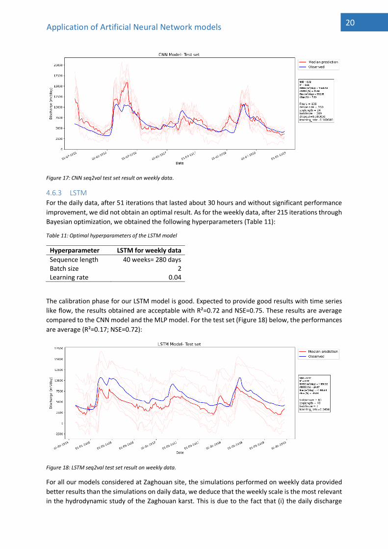
20 Application of Artificial Neural Network models
Figure 17: CNN seq2val test set result on weekly data.
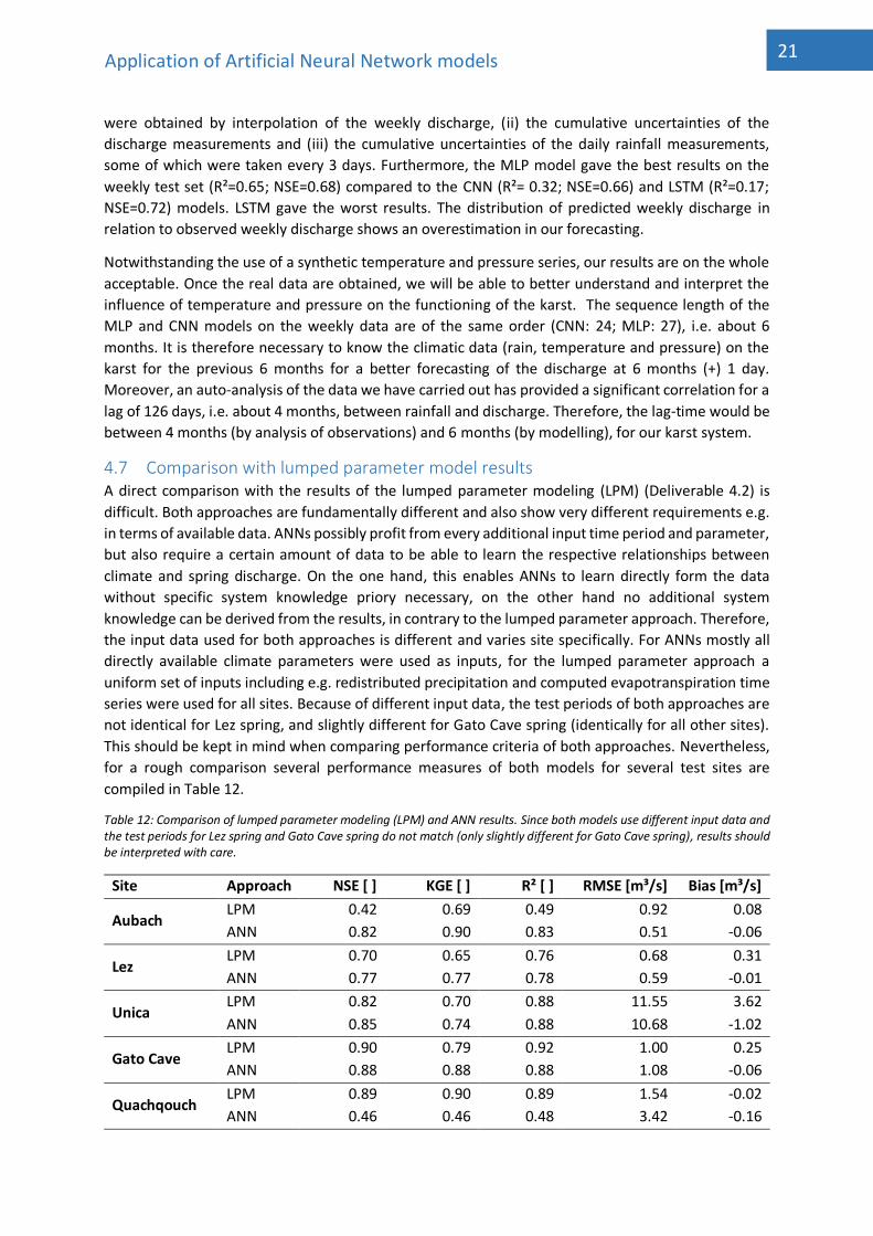
4.6.3 LSTM For the daily data, after 51 iterations that lasted about 30 hours and without significant performance
improvement, we did not obtain an optimal result. As for the weekly data, after 215 iterations through
Bayesian optimization, we obtained the following hyperparameters (Table 11):
Table 11: Optimal hyperparameters of the LSTM model
Hyperparameter LSTM for weekly data
Sequence length 40 weeks= 280 days Batch size 2 Learning rate 0.04
The calibration phase for our LSTM model is good. Expected to provide good results with time series
like flow, the results obtained are acceptable with R²=0.72 and NSE=0.75. These results are average
compared to the CNN model and the MLP model. For the test set (Figure 18) below, the performances
are average (R²=0.17; NSE=0.72):
Figure 18: LSTM seq2val test set result on weekly data.
For all our models considered at Zaghouan site, the simulations performed on weekly data provided
better results than the simulations on daily data, we deduce that the weekly scale is the most relevant
in the hydrodynamic study of the Zaghouan karst. This is due to the fact that (i) the daily discharge
21 Application of Artificial Neural Network models
were obtained by interpolation of the weekly discharge, (ii) the cumulative uncertainties of the
discharge measurements and (iii) the cumulative uncertainties of the daily rainfall measurements,
some of which were taken every 3 days. Furthermore, the MLP model gave the best results on the
weekly test set (R²=0.65; NSE=0.68) compared to the CNN (R²= 0.32; NSE=0.66) and LSTM (R²=0.17;
NSE=0.72) models. LSTM gave the worst results. The distribution of predicted weekly discharge in
relation to observed weekly discharge shows an overestimation in our forecasting.
Notwithstanding the use of a synthetic temperature and pressure series, our results are on the whole
acceptable. Once the real data are obtained, we will be able to better understand and interpret the
influence of temperature and pressure on the functioning of the karst. The sequence length of the
MLP and CNN models on the weekly data are of the same order (CNN: 24; MLP: 27), i.e. about 6
months. It is therefore necessary to know the climatic data (rain, temperature and pressure) on the
karst for the previous 6 months for a better forecasting of the discharge at 6 months (+) 1 day.
Moreover, an auto-analysis of the data we have carried out has provided a significant correlation for a
lag of 126 days, i.e. about 4 months, between rainfall and discharge. Therefore, the lag-time would be
between 4 months (by analysis of observations) and 6 months (by modelling), for our karst system.
4.7 Comparison with lumped parameter model results A direct comparison with the results of the lumped parameter modeling (LPM) (Deliverable 4.2) is
difficult. Both approaches are fundamentally different and also show very different requirements e.g.
in terms of available data. ANNs possibly profit from every additional input time period and parameter,
but also require a certain amount of data to be able to learn the respective relationships between
climate and spring discharge. On the one hand, this enables ANNs to learn directly form the data
without specific system knowledge priory necessary, on the other hand no additional system
knowledge can be derived from the results, in contrary to the lumped parameter approach. Therefore,
the input data used for both approaches is different and varies site specifically. For ANNs mostly all
directly available climate parameters were used as inputs, for the lumped parameter approach a
uniform set of inputs including e.g. redistributed precipitation and computed evapotranspiration time
series were used for all sites. Because of different input data, the test periods of both approaches are
not identical for Lez spring, and slightly different for Gato Cave spring (identically for all other sites).
This should be kept in mind when comparing performance criteria of both approaches. Nevertheless,
for a rough comparison several performance measures of both models for several test sites are
compiled in Table 12.
Table 12: Comparison of lumped parameter modeling (LPM) and ANN results. Since both models use different input data and the test periods for Lez spring and Gato Cave spring do not match (only slightly different for Gato Cave spring), results should be interpreted with care.
Site Approach NSE [ ] KGE [ ] R² [ ] RMSE [m³/s] Bias [m³/s]
Aubach LPM 0.42 0.69 0.49 0.92 0.08
ANN 0.82 0.90 0.83 0.51 -0.06
Lez LPM 0.70 0.65 0.76 0.68 0.31
ANN 0.77 0.77 0.78 0.59 -0.01
Unica LPM 0.82 0.70 0.88 11.55 3.62
ANN 0.85 0.74 0.88 10.68 -1.02
Gato Cave LPM 0.90 0.79 0.92 1.00 0.25
ANN 0.88 0.88 0.88 1.08 -0.06
Quachqouch LPM 0.89 0.90 0.89 1.54 -0.02
ANN 0.46 0.46 0.48 3.42 -0.16

22 Application of Artificial Neural Network models
The results of the ANN based modeling are mostly better than for the LPM approach. Especially for
modeling the complex Aubach spring system, ANNs clearly outperform the LPM model. Similarly, ANNs
show better results at Lez spring, however the test periods do not match here, which makes a
comparison difficult. No clear differences can be found at Unica springs and Gato Cave spring, where
partly ANN and partly LPM show better performance. Unica spring is directly comparable, but also at
Gato Cave spring the test period is almost identical. The Qachqouch results demonstrate the
advantages of LPMs that need less data (in terms of length of the data period) to successfully model a
karst spring system. While ANNs fail here, the LPM shows rather good results.
5 Conclusions The results show that the 1D-CNN approach can be easily implemented to successfully and accurately
model karst spring discharge under different climatic conditions, as long as a sufficient amount of
historical data (discharge, climatic inputs) is available to train the model. It is possible to model systems
showing significant different properties such as catchment size, complexity and hydraulic properties.
Four out of five springs were modeled with good to very high accuracy, only for Qachqouch spring the
approach was not successful, most certainly because of insufficient data availability for both climatic
inputs and spring discharge. The chosen approach is adaptable to specific data properties as the
example of Lez spring show. Here the modeler can easily teach that negative discharge values are
forbidden and hence can increase physical meaning of the modeling. This is in principle true for all
spring discharge time series, as negative discharge is not possible, however as long as the (close-to-)
zero discharge is natural (which is not the case for Lez spring), the model usually learns this relation by
itself reliably. It can be concluded that for a mere simulation purpose, the CNN approach is associated
with comparably low effort and a legitimate alternative to conventional model approaches such as
lumped parameter modeling. At Zaghouan site the CNN approach was outperformed by a MLP model
(on weekly timescale), which, however, showed strong dependency on the random seed initialization.
Here, the CNN again showed that it is more stable than other approaches.
References Abadi, M., Agarwal, A., Barham, P., Brevdo, E., Chen, Z., Citro, C., Corrado, G.S., Davis, A., Dean, J., Devin, M., Ghemawat, S.,
Goodfellow, I., Harp, A., Irving, G., Isard, M., Jia, Y., Jozefowicz, R., Kaiser, L., Kudlur, M., Levenberg, J., Mane, D., Monga, R., Moore, S., Murray, D., Olah, C., Schuster, M., Shlens, J., Steiner, B., Sutskever, I., Talwar, K., Tucker, P., Vanhoucke, V., Vasudevan, V., Viegas, F., Vinyals, O., Warden, P., Wattenberg, M., Wicke, M., Yu, Y., Zheng, X., 2015. TensorFlow: Large-Scale Machine Learning on Heterogeneous Distributed Systems 19.
Bergström, S., 1995. The HBV model, in: Singh, V.P. (Ed.), Computer Models of Watershed Hydrology. Water Resources Publications, Colorado, USA, pp. 443–476.
Bergström, S., 1975. The development of a snow routine for the HBV-2 model. Hydrol. Res. 6, 73–92. https://doi.org/10/gkcqz5
Chen, Z., Auler, A.S., Bakalowicz, M., Drew, D., Griger, F., Hartmann, J., Jiang, G., Moosdorf, N., Richts, A., Stevanovic, Z., Veni, G., Goldscheider, N., 2017a. The World Karst Aquifer Mapping project: concept, mapping procedure and map of Europe. Hydrogeol. J. 25, 771–785. https://doi.org/10/f98h6g
Chen, Z., Hartmann, A., Goldscheider, N., 2017b. A new approach to evaluate spatiotemporal dynamics of controlling parameters in distributed environmental models. Environ. Model. Softw. 87, 1–16. https://doi.org/10.1016/j.envsoft.2016.10.005
Chen, Z., Hartmann, A., Wagener, T., Goldscheider, N., 2018. Dynamics of water fluxes and storages in an Alpine karst catchment under current and potential future climate conditions. Hydrol Earth Syst Sci 17. https://doi.org/10.5194/hess-22-3807-2018
Chollet, F., 2015. Keras. Faydi, T., 2021. La modélisation hydrodynamique des aquifères karstiques de Djebel Zaghouan par karstmod. Mastère de
Recherche spécialité : Modélisation en Hydraulique et Environnement. ENIT, Tunis. Gupta, H.V., Kling, H., Yilmaz, K.K., Martinez, G.F., 2009. Decomposition of the mean squared error and NSE performance
criteria: Implications for improving hydrological modelling. J. Hydrol. 377, 80–91. https://doi.org/10.1016/j.jhydrol.2009.08.003
Hock, R., 1999. A distributed temperature-index ice- and snowmelt model including potential direct solar radiation. J. Glaciol. 45, 101–111. https://doi.org/10/ggnvkt

23 Application of Artificial Neural Network models
Hunter, J.D., 2007. Matplotlib: A 2D Graphics Environment. Comput. Sci. Eng. 9, 90–95. https://doi.org/10.1109/mcse.2007.55
Jeannin, P.-Y., Artigue, G., Butscher, C., Chang, Y., Charlier, J.-B., Duran, L., Gill, L., Hartmann, A., Johannet, A., Jourde, H., Kavousi, A., Liesch, T., Liu, Y., Lüthi, M., Malard, A., Mazzilli, N., Pardo-Igúzquiza, E., Thiéry, D., Reimann, T., Schuler, P., Wöhling, T., Wunsch, A., 2021. Karst modelling challenge 1: Results of hydrological modelling. J. Hydrol. 600, 126508. https://doi.org/10.1016/j.jhydrol.2021.126508
Johannet, A., Mangin, A., D’Hulst, D., 1994. Subterranean water infiltration modelling by neural networks: use of water source flow, in: ICANN ’94: Proceedings of the International Conference on Artificial Neural Networks Sorrento, Italy, 26–29 May 1994 Volume 1, Parts 1 and 2. Presented at the International Conference on Artificial Neural Networks, Springer Berlin Heidelberg, Sorrento, Italy, pp. 1033–1036.
Kollat, J.B., Reed, P.M., Wagener, T., 2012. When are multiobjective calibration trade-offs in hydrologic models meaningful? Water Resour. Res. 48. https://doi.org/10/gkcq5k
Kong-A-Siou, L., Johannet, A., Borrell Estupina, V., Pistre, S., 2015. Neural networks for karst groundwater management: case of the Lez spring (Southern France). Environ. Earth Sci. 74, 7617–7632. https://doi.org/10.1007/s12665-015-4708-9
Lebigot, E.O., 2010. Uncertainties: a Python package for calculations with uncertainties. LeCun, Y., Bengio, Y., Hinton, G., 2015. Deep learning. Nature 521, 436–444. https://doi.org/10.1038/nature14539 Mbah, T.J., Ye, H., Zhang, J., Long, M., 2021. Using LSTM and ARIMA to Simulate and Predict Limestone Price Variations. Min.
Metall. Explor. 38, 913–926. https://doi.org/10/gmhg5w McKinney, W., 2010. Data Structures for Statistical Computing in Python. Presented at the Python in Science Conference,
Austin, Texas, pp. 56–61. https://doi.org/10.25080/majora-92bf1922-00a Nash, J.E., Sutcliffe, J.V., 1970. River flow forecasting through conceptual models part I—A discussion of principles. J. Hydrol.
10, 282–290. https://doi.org/10.1016/0022-1694(70)90255-6 Nogueira, F., 2014. Bayesian Optimization: Open source constrained global optimization tool for Python. Pedregosa, F., Varoquaux, G., Gramfort, A., Michel, V., Thirion, B., Grisel, O., Blondel, M., Prettenhofer, P., Weiss, R., Dubourg,
V., Vanderplas, J., Passos, A., Cournapeau, D., 2011. Scikit-learn: Machine Learning in Python. J. Mach. Learn. Res. 12, 2825–2830.
Reback, J., McKinney, W., Jbrockmendel, Bossche, J.V.D., Augspurger, T., Cloud, P., Gfyoung, Sinhrks, Klein, A., Roeschke, M., Hawkins, S., Tratner, J., She, C., Ayd, W., Terji Petersen, Garcia, M., Schendel, J., Hayden, A., MomIsBestFriend, Jancauskas, V., Battiston, P., Skipper Seabold, Chris-B1, H-Vetinari, Hoyer, S., Overmeire, W., Alimcmaster1, Kaiqi Dong, Whelan, C., Mortada Mehyar, 2020. pandas-dev/pandas: Pandas 1.0.3. Zenodo. https://doi.org/10.5281/ZENODO.3509134
Sagna, J., 2000. Study and modeling of Zaghouan karst sources, Master thesis. ENIT. Seibert, J., 2000. Multi-criteria calibration of a conceptual runoff model using a genetic algorithm. Hydrol. Earth Syst. Sci. 4,
215–224. https://doi.org/10/crmzd7 Shanker, M., Hu, M.Y., Hung, M.S., 1996. Effect of data standardization on neural network training. Omega 24, 385–397.
https://doi.org/10/ck4tv5 van der Walt, S., Colbert, S.C., Varoquaux, G., 2011. The NumPy Array: A Structure for Efficient Numerical Computation.
Comput. Sci. Eng. 13, 22–30. https://doi.org/10.1109/mcse.2011.37 van Rossum, G., 1995. Python tutorial. Wunsch, A., Liesch, T., Broda, S., 2021. Groundwater level forecasting with artificial neural networks: a comparison of long
short-term memory (LSTM), convolutional neural networks (CNNs), and non-linear autoregressive networks with exogenous input (NARX). Hydrol. Earth Syst. Sci. 25, 1671–1687. https://doi.org/10.5194/hess-25-1671-2021
Copyright © 2022 FDOKUMEN