Marine Chemistry 122 (2010) 20–27

Contents lists available at ScienceDirect

Marine Chemistry

j ourna l homepage: www.e lsev ie r.com/ locate /marchem

Significant portion of dissolved organic Fe complexes in fact is Fe colloids

Marie Boye a,⁎,1, Jun Nishioka b, Peter Croot a,2, Patrick Laan a, Klaas R. Timmermans a, Volker H. Strass c,Shigenobu Takeda d, Hein J.W. de Baar a

a Royal Netherlands Institute for Sea Research (NIOZ), Postbus 59, 1790 AB Den Burg, Texel, The Netherlandsb Hokkaido University, Institute of Low Temperature Science, Sapporo 060-0819, Japanc Alfred-Wegener-Institut für Polar und Meeresforschung, Bremerhaven, Germanyd University of Tokyo, Department of Aquatic Bioscience, Bunkyo, Tokyo 113-8657, Japan

⁎ Corresponding author. Tel.: +33 2 98 49 86 51; faxE-mail address: marie.boye@univ-brest.fr (M. Boye)

1 Now at Laboratoire des Sciences de l'EnvironneUMR6539, Institut Universitaire Européen de la Mer, TPlouzane, France.

2 Now at: Forschungsbereich Marine BiogeochemiLeibniz-Institut für Meereswissenschaften, DienstgebäuWeg 20, 24105 Kiel, Germany.

0304-4203/$ – see front matter © 2010 Elsevier B.V. Adoi:10.1016/j.marchem.2010.09.001

a b s t r a c t

a r t i c l e i n f o

Article history:Received 20 August 2009Received in revised form 23 August 2010Accepted 5 September 2010Available online 16 September 2010

Keywords:IronSize fractionationComplexationSouthern Ocean

Vertical distributionsof iron and ironbinding ligandsweredetermined in2 size classes (dissolvedb0.2 μm,solubleb200 kDa, e.g., ~0.03 μm) in the Southern Ocean. Colloidal iron and complexing capacity (N200 kDa–b0.2 μm)were inferred as the difference between the dissolved and soluble fractions. Dissolved iron and ligands existprimarily in the soluble size range in the surface waters, although iron-complexing colloids still represent asignificant portion of the dissolved pool and this fraction increases markedly with depth. This work presentsevidence for the colloidal nature of a significant portion (37–51% on average) of the ‘dissolved’ organic Fe pool inthese oceanic waters. From the data it was not possible to discern whether iron colloids exist as discrete organiccomplexes and/or inorganic amorphous colloids. Iron-complexing colloids are themost saturatedwith iron at thethermodynamic equilibrium, whereas soluble organic ligands occur in larger excess compared to soluble iron. Itsuggests that the exchangeable fraction for iron uptake through dissociation of Fe complexes likely occurs inthe soluble fraction, and that soluble ligands have the potential to buffer iron inputs to surface waters whereasiron colloids may aggregate and settle. Expectations based on Fe diffusion rates, distributions and the stabilityof the soluble iron complexes and iron colloids also suggest that the weaker soluble Fe complexes may be morebio-available, while the strongest colloids may be a major route for iron removal from oceanic waters.Investigations of the size classes of the dissolved organic iron thus can significantly increase our understanding ofthe oceanic iron cycle.

: +33 2 98 49 86 45..ment Marin (LEMAR), CNRSechnopole Brest-Iroise, 29280

e, Chemische Ozeanographie,de Westufer, Düsternbrooker

ll rights reserved.

© 2010 Elsevier B.V. All rights reserved.

1. Introduction

There is now compelling evidence to demonstrate that dissolvediron is principally complexed by organic ligands in oceanic waters(Gledhill and van den Berg, 1994; van den Berg, 1995; Rue andBruland, 1995; Boye et al., 2001). The organic complexation is acentral factor in oceanic iron cycling by controlling iron solubility (Wuand Luther, 1995) and selective iron bio-availability (Hutchins et al.,1999), but the speciation and the oceanic cycling of the organicchelators are still poorly understood. It has become increasinglyrecognized that a myriad of organic Fe-binding structures will coexistin oceanic waters. Recent studies also have shown that dissolved ironoccurs in soluble and colloidal fractions which have importantimplications for the iron cycle in the ocean (Nishioka et al., 2003;

Bergquist et al., 2007; Wu et al., 2001). However, only a few studieshave examined the size-spectrum of the dissolved organic ligands inoceanic waters (Wu et al., 2001; Cullen et al., 2006; Boye et al., 2005;Kondo et al., 2008). The first profiles of both soluble iron and ironbinding organic ligands (b0.02 μm) from the North Atlantic and NorthPacific exhibited a nutrient-like profile (Wu et al., 2001). By contrastcolloidal iron (N0.02–b0.4 μm) showed a maximum at the nearsurface and aminimum in the nutricline in these oceanic basins whereiron may be bound to organic ligands present in the colloidal sizerange (Wu et al., 2001). Similar distributions of soluble and colloidalligands have been observed in the Western Atlantic basin (Cullenet al., 2006). Lately a first complete description of the physical andchemical speciation of dissolved iron and Fe-binding ligands wasrecorded in iron-enriched waters during a mesoscale iron enrichmentin the open Southern Ocean (EISENEX) (Boye et al., 2005; Nishiokaet al., 2005; Croot et al., 2005). This work showed that the added ironexisted principally as colloids (N200 kDa–b0.2 μm) in the surfaceenriched waters (Nishioka et al., 2005) similar to the newly producedligands (Boye et al., 2005), but the organic nature of colloidal ligandsand its complexes with iron was not certain in this experiment (Boyeet al., 2005). By contrast most of the increase of the dissolved Fe-binding ligands observed during a mesoscale iron enrichment

21M. Boye et al. / Marine Chemistry 122 (2010) 20–27

experiment in the western subarctic North Pacific (SEEDS II) wasattributable to the soluble fraction (Kondo et al., 2008), possiblydepicting differences in ambient water-masses chemistry, physics andbiological features. The discrete size classes of dissolved iron couldimpact the iron cycling in different ways since colloidal iron-speciesmay be more chemically dynamic (Boye et al., 2005; Nishioka et al.,2005) hence controlling iron removal from the surface waters (Wuet al., 2001) and possibly in deep waters with implication in the inter-basin fractionation (Bergquist et al., 2007), although truly solubleiron-species may be more bio-available, controlling then the primaryproducers community structure (Wu et al., 2001).

Here we report the vertical distribution of size-fractionateddissolved (b0.2 μm) iron and its ligands (soluble b200 kDa, and200 kDabcolloidalb0.2 μm) in the ambient waters of the SouthernPolar Frontal Zone to investigate the size-partitioning of the so-called‘dissolved’ organic iron.

2. Methods

Filtered (b0.2 μm) and ultrafiltered (b200 kDa) seawater wascollected between 0 and 1000 m depth in the Atlantic sector of theSouthern Ocean (along the 20–21°E meridian, between latitudes47.7°S and 49.3°S) in late spring (November 2–25th 2000) on board ofthe Research Vessel Polarstern (cruise ANTXVIII/2, also referred as the“EISENEX” Fe-enrichment experiment). Samples were collected usingacid-cleaned Teflon coated Go-Flo bottles suspended on a Kevlar wire(Croot et al., 2005). Filtered samples (b0.2 μm; Sartorius Sartobranfilter capsule) were collected in low density polyethylene (LDPE)bottles for iron and the ligands determination. Additional filtrate(b0.2 μm) samples collected into acid-cleaned 500 ml polycarbonatewere immediately size-fractionated by a clean inline ultrafiltrationsystem using a 200 kDa (~0.03 μm) polyethylene hollow-fiberultrafilter unit (Sterapore) under a laminar flow clean air hoodaboard (Nishioka et al., 2005). The smaller fraction (b200 kDa) wascollected in acid-cleaned low density polyethylene bottles for iron andthe ligands analyses. Then for both iron and the ligands, operationaldefinitions were taken as “dissolved” being the filtrate b0.2 μm, and“soluble” being the ultrafiltrate b200 kDa. The “colloidal” fraction wasobtained as the difference calculated between these two fractions(e.g., 200 kDa bcolloidal b0.2 μm). In this sampling procedure itcannot be excluded that the soluble Fe fractionmay include some verysmall colloids (Nishioka et al., 2001; Wells et al., 1998), henceintroducing underestimation of the colloidal Fe fraction. Furthermorethe colloidal fractions of both iron and the ligands are estimated bydifference between the analyses of the dissolved and the solublefractions, rather than a direct measurement from the retentate of theultrafiltration. Such procedures and calculations have been usedpreviously to estimate colloidal Fe (Nishioka et al., 2001, 2003, 2005;Wu et al., 2001; Cullen et al., 2006; Bergquist et al., 2007) and the Fe-complexing ligands in the small size-spectrum (Wu et al., 2001; Boyeet al., 2005; Cullen et al., 2006; Kondo et al., 2008).

Dissolved and soluble iron concentrations were determined asFe(III)-species with an automatic flow injection analytical system(Kimoto Electric, Ltd.) using concentration onto an 8-hydroxyqui-noline chelating column, recovered after acidification at pH 3.2 andchemiluminescence detection (Obata et al., 1993). More recentlythe SAFE cruise has shown that the iron concentrations with suchacidification procedure yielded slightly lower values than thoseafter acidifying at pH less than 1.8 (Johnson et al., 2007). Themethod and most of the ambient size-fractionated iron concentra-tions are described in detail in Nishioka et al. (2005). The detectionlimit (three times the standard deviation) of Fe(III) concentrationsfor purified seawater (seawater passed through 8-hydroxyquinolineresin column three times) on this cruise was 15–32 pM (Nishiokaet al., 2005). The relative coefficient of variation was within 5%(n=12) for replicate measurements of a seawater sample contain-

ing 0.53 nM Fe(III), within 6% (n=9) for 5.3 nM Fe(III) (Nishiokaet al., 2005). The relative standard deviation of the filtration methodwith polyethylene hollow-fiber ultrafilter was 11% for replicatefiltration of a seawater sample containing 0.1 nM Fe(III) and 9% forreplicate filtration of a seawater sample containing 0.8 nM Fe(III).Dissolved and soluble iron concentrations were used to estimatethe organic speciation in the dissolved and soluble size-fractionsrespectively.

The organic complexation of ironwasdetermined aboard the ship bycomplexing capacity titrations in the dissolved and the soluble filtrates,using cathodic stripping voltammetry (CSV) with ligand competitionagainst 2-(2-thiazolylazo)-p-cresol (TAC) (Croot and Johansson, 2000).The methodologies and procedures employed in this work are fullydescribed in Boye et al. (2005). Briefly, 220 ml aliquot of seawater wasbufferedwith 5 mMof borate buffer, followed by addition of 10 μMTAC.After mixing eleven 20 ml aliquots of sample were pipetted into Teflonvials spiked with increasing additions of iron. After an overnightequilibration labile iron concentrations were determined by CSV.Voltammetric conditions used were as follows: a 200 s N2 purge; a−0.4 V adsorption potential for 200–400 s; a quiescent period of 10 s;and a fast linear sweep waveform scanning mode using a scan rate of10 V s−1. Using this procedure the detection limit (3 times the standarddeviation) of the CSV iron analyses in clean seawater was 30 pM (Boyeet al., 2005). The standard deviations of the ligand concentrations (L)and the conditional stability (K′FeIIIL) constants were calculated fromlinear least-square regression of the titration curves fitted for a singleligands group (Boye et al., 2001). The relative standard deviation(precision) of repeated determinations of the ligand concentration wasbetter than 5% and better than 1% for the conditional stability constant(Boye et al., 2005).

3. Results and discussion

3.1. Study area

The four sampling stations were geographically located within thebroad eastward-flowing Antarctic Circumpolar Current (ACC) north ofthe Antarctic Polar Front (APF) that had its major jet centered atroughly 49°30′S (Strass et al., 2001). However, at stations 9, 48 and 91in the latitude range 47°49′S–48°36′S a subsurface temperatureminimum layer was observed at around 180–200 m depth bound bythe 2 °C isotherm, characteristic of Antarctic Winter Water (Belkinand Gordon, 1996) (Figs. 1–2). Furthermore the horizontal currentsmeasured with a VM-ADCP at these stations (Strass et al., 2001)showed vanishingly low or even westward currents. The WinterWater and current pattern indicated that the three stations werelocated within a cyclonic eddy, which likely had shed from the APF bydetachment from a northward protruding meander (Cisewski et al.,2005). The vertical mixing in the eddy and its evolution in the courseof the EISENEX experiment werewell studied since the eddy served asthe hydrographic structure for the three iron infusions (Cisewski et al.,2005). From the relative position of the stations and the eddy core,station 9 was located in the center of the eddy before the first ironrelease, station 48 was on the edge of the eddy on its southernbottleneck one day after the second Fe-release, and station 91 wassampled in the eddy on the edge of the second infused patch about tendays after the second Fe-release and about 3–4 days after a secondstorm had crossed the patch area. The temperature in the subsurfacetemperature minimum at station 7 (Figs. 1–2) was above 2 °C, relatedto the fact that this station was located north of the Antarctic PolarFront but outside and to the south of the eddy.

The eddy carried with it the nutrients signature of the watersoriginating from the southern side of the APF, with a high surfaceresidual level of nitrate (22–24 μM)and relatively higher surface silicatelevels (12–14 μM) compared to station 7 located outside of the eddy(9 μM) (Fig. 3). The mixed layer depth generally deepened with time

Salinity

34.0 34.4 34.8

Dep

th (

m)

0

200

400

600

800

1000

St.007

St.009

St.048

St.091

Temperature (°C)

1 2 3 4

Fig. 1. Salinity and temperature profiles in the top 1100 m recorded at stations #007 (49.29°S, 20.02°E), #009 (47.82°S, 20.79°E), #048 (48.59°S, 20.72°E), and #091 (48.17°S,21.09°E). (CTD data recording and validation as described by Strass et al., 2001.)

22 M. Boye et al. / Marine Chemistry 122 (2010) 20–27

(~20 m at station 7, and from ~30 m at station 9 and station 48 to 90 mmixed layer depth at station 91 in the eddy; Fig. 1). Chlorophyll-adisplayed relative concentration maxima in the upper 100 m (Fig. 3),with lower mean values outside of the eddy (e.g.; 0.33 μg l−1 at station7) compared to inside the eddy (e.g.; 0.52 μg l−1 at station 9 and0.73 μg l−1 at station 91) and on its edge (e.g.; 0.54 μg l−1 at station 48)(Gervais et al., 2002). The pico- (b2 μm) and nano-phytoplankton (2–20 μm) dominated the phytoplankton assemblage in these watersaccounting for 28–39% and 42–52% of Chl-a respectively (Gervais et al.,2002).

The chlorophyll-a levels at stations located inside the Fe-patch afterthe second infusion, immediately prior to sampling the out-patchstations, displayed much higher mean concentrations (e.g., 1.26 μg l−1

at station 46, and 1.64 μg l−1 at station 88) compared to station 48(0.55 μg l−1) and station 91 (0.73 μg l−1), respectively. No storm orprecipitation events occurred between the respective in- and out-patchstations that could have caused a dilution of the Fe-fertilized watercharacteristics. This suggests that the top 200 m of stations 48 and 91was unlikely imprinted by the biogeochemical signals of the second ironinfusion, hence they featured the eddy waters that originated from thesouthern side of the Antarctic Polar Front as for station 9.

3.2. The size-spectrum of dissolved iron

The ultrafiltration procedure of soluble iron and the calculationmode of colloidal iron may have introduced sampling bias since

T (°C)

1 2 3 4

Sal

inity

33.8

34.0

34.2

34.4

34.6

34.8

St.007St.009St.048St.091

Fig. 2. Temperature–salinity diagram in the top 1100 m at stations #007 (49.29°S,20.02°E), #009 (47.82°S, 20.79°E), #048 (48.59°S, 20.72°E), #091 (48.17°S, 21.09°E).(CTD data recording and validation as described by Strass et al., 2001.)

colloidal Fe could be formed or adsorbed onto the filter during theultrafiltration step or on the contrary could solubilize. Comparisonsbetween microfiltration methods and cross flow filtration (using themethod described in Wen et al., 2000) however did not show anysignificant difference in the colloidal Fe concentrations even at lowlevels such as 90 pM (Wu et al., 2001), indicating that colloidal Febased on the difference of Fe concentrations analysed in the dissolvedand soluble fractions is likely due to particulate retention rather thanFe adsorption/desorption by the ultrafilter (Wu et al., 2001). Goodmass balances for Fe were also obtained using a cross flow filtrationsystem employed with a 10 kDa membrane in typical oceanic waters(Schlosser and Croot, 2008). The colloidal Fe concentrations calculatedhere as the difference between the dissolved and soluble fractions are2–12 and 3–25 times higher than the 5% precision of dissolved Fe andsoluble Fe concentrations, respectively (Table 1), suggesting goodreliability of the estimation of the colloidal fraction. Furthermorepaired two-tailed t-test shows that the differences between dissolvedand soluble Fe, equivalent to colloidal Fe, are statistically significant atthe 95% confident interval (P=0.05, tcritical=1.72, texperimental=4.45,n=22).

Dissolved Fe and soluble Fe roughly exhibit nutrient-like profiles(Fig. 4), with depleted concentrations in surface waters (mean valuesrespectively, 65±18, 43±14 pM) and increasing concentrations indeeper waters below the Antarctic Winter Water (230±100, 130±40 pM respectively). Colloidal Fe concentrations are much lower insurface waters (mean value, 23±9 pM) compared to soluble Fesuggesting that colloidal iron may be more efficiently removed fromsurface waters than soluble iron (Fig. 4). In deeper waters colloidaliron gradually increases (mean value, 100±60 pM) (Fig. 4). Despitestation 7 being located outside of the eddy, the two data pointsgathered at 50 m and 1000 m at this station are in the same rangethan the concentrations recorded at the other stations, located withinthe eddy (Table 1). The data indicate that dissolved Fe is principallypresent in the soluble size range in the surface waters (accounting for63±8% of dissolved Fe), while in deeper waters below 500 m thecolloidal and soluble Fe portions of dissolved Fe are almost equallybalanced (51 and 49% respectively). Based onmolecular diffusion rateof spherical species through liquid that is inversely related to theirradius (Einstein–Stokes relation), soluble Fe (size b~30 nm) should bemore available for phytoplankton uptake than colloidal Fe species(diameters ~30–200 nm), provided the uptake is limited solely bydiffusion of Fe species to the cell surface. Furthermore diffusionlimitation increases markedly with increasing cells size or cells-aggregates size (Timmermans et al., 2004). Diffusion limitation may

22 24 26 28 30

Dep

th (

m)

0

100

200

300

St.007

St.009

St.048

St.091

[Si] (µmol l-1)7 14 21 28

[NO3] (µmol l-1) [Chl-a] (µg l-1)0.0 0.2 0.4 0.6 0.8

Fig. 3. Nitrate, silicate (Hartmann et al., 2001; Kattner, 2009) and chlorophyll-a (Riebesell et al., 2001) concentrations in the top 300 m at stations #007 (49.29°S, 20.02°E), #009(47.82°S, 20.79°E), #048 (48.59°S, 20.72°E), and #091 (48.17°S, 21.09°E).

23M. Boye et al. / Marine Chemistry 122 (2010) 20–27

thus be less severe for pico- and nano-phytoplankton that dominatethe phytoplankton assemblage in these waters (Gervais et al., 2002)than for other typical austral large (chain-forming) diatom specieslike Fragilariopsis kerguelensis (individual cells 60 μm long, 20 μmwide). In turn biological uptake of soluble Fe by the smallestphytoplankton combined with low Fe inputs in the surface waters,and possibly aggregation and settling or particles scavenging ofcolloidal iron similar to Th isotopes (Savoye et al., 2006), accompaniedby the releases of both soluble and colloidal Fe in the twilight zone byremineralisation of sinking particles and by desorption hence couldcreate the dissolved Fe profiles observed in these polar waters (Fig. 4).

Despite lower abundance, colloidal Fe still comprised ~37% of thedissolved Fe fraction in the surface waters. This value is slightly higherthan in surface layers of the subarctic (~23%) and equatorial (~15%)Pacific (Nishioka et al., 2001, 2003; Wells, 2003), but substantiallylower than what is reported for the near-surface waters of the northAtlantic and Pacific (80–90%) (Wu et al., 2001), for the surface watersof the north western Atlantic (65–90%) (Cullen et al., 2006), and forartificially Fe-enriched surface waters of the austral PFZ (~76%)(Nishioka et al., 2005) and of the northwestern subarctic Pacific(~64%) (Kondo et al., 2008). Differences in fractionation methodol-ogies can cause these differences (Wells, 2003). It is also likely that thedifferent Fe supplies (e.g., atmospheric sources, upwelling, artificial Fesupply, and lithogenic sources) in these areas can influence thecolloidal Fe percentage (Nishioka et al., 2005).

3.3. The size-spectrum of dissolved ligands

The colloidal ligand concentrations calculated as the differencebetween the dissolved and soluble fractions are occasionally within(at three surface waters data points), but mostly well above (by 2 to11 times), the 5% precision of dissolved L and soluble L concentrations(Table 1), suggesting that these values are not artifacts of thecalculation method. The paired two-tailed t-test also shows that thedifferences between dissolved and soluble L (e.g., equivalent tocolloidal L) are statistically significant at the 95% confident interval(P=0.05, tcritical=1.73, texperimental=7.48, n=20). Furthermore thedata points recorded at station 7 located outside of the eddy comparedwell with the ligands concentrations observed at similar depths in theeddy (Table 1).

Dissolved L and soluble L distributions suggest a biological source insurfacewaterswith relativemaxima at thebase of the chlorophyll-a richlayer (maximum value, 0.9 nM, 0.8 nM, respectively), and a fairlyconstant distribution in deeper waters (mean values of 0.70±0.07 and

0.50±0.05 nM respectively) (Fig. 5). The two samples taken at 300 and400 mdepth at station 9however deviate somewhat from this generallyhomogenous distribution in that soluble ligand here makes a compa-rably higher contribution to the dissolved ligand pool, and is probablyrelated to the fact that station9 in the center of theeddy features also thecoldest water in that depth range, e.g., water from the most southerlyorigin (Fig. 1). By contrast iron-complexing colloids do not show amaximum in surface waters, but its concentration gradually increaseswith depth in the mesopelagic zone (from minimal values of 0.06±0.02 nM in surface waters up to 0.15±0.06 nM below the AntarcticWinter Water core) (Fig. 5). Thereby the vertical distribution of Fe-complexing colloids is possibly driven by its aggregation and settlingand/or its particle scavenging (adsorption to and removal on sinkingparticles) from the upper ocean, and its release in deeper waters byremineralisation, disaggregation and by desorption from particles. Thedata indicate that dissolved ligands are mainly present in the solublesize range in the surface waters (representing 91±2% of dissolved L),although iron-complexing colloids abundance increases significantly indeeper waters (accounting for 13–35% of the dissolved pool below200 m, compared to 4–12% in the surface layer). Consequently the ratio[Lsol]/[Lcoll] is much higher in surface waters (~13) compared to deeperwaters below 200 m (~4). Biological production of soluble ligands insurface waters and removal of iron-complexing colloids from the upperlayer may hence drive the distribution of dissolved ligands in thesewaters. In deeper waters regeneration of sinking material, bacterialdecomposition and possibly desorption from particles may supplyrelatively more colloids compared to soluble ligands. Regeneration ofsinking biogenic particulate organic material is thought to be animportant source for soluble L in thenorthAtlantic andPacific (Wuet al.,2001).

No significant difference in the conditional stability constant ofdissolved iron complexes (LogK′FeL-diss) was depicted between thesurface (~21.95) and the deeper waters (~21.98) (Table 1), and only asingle ligand group was evident from the resolution of the titrationcurves of the dissolved ligands by applying the linear least-squaresregressions. It means that the small size-spectrum could not beresolved by applying CSV titration method in the dissolved fractionalone, and that ultrafiltration is required to discriminate the ligandsby size.

3.4. The complexation of dissolved iron in the small size-fractions

Soluble and colloidal Fe may be present principally bound tosoluble ligands and colloidal ligands respectively. Soluble L are indeed

Table 1Concentrations of iron and Fe-binding ligands measured in the dissolved (b0.2 μm) and soluble (b200 kDa) fractions at 4 stations in the Southern Ocean during the ANTXVIII/2 (EISENEX) expedition. The colloidal iron and ligandconcentrations were calculated as the difference between the dissolved (b0.2 μm) and the soluble (b200 kDa) fractions. The standard deviation of iron (sdv) was calculated using the relative coefficient of variation of the measurement (equalto 5%; see text). The conditional stability constants of the iron(III)–ligand complexes (LogK′) were calculated by linear least-squares regression of the titration fitted for a linear equation (Ruzic, 1982). The standard deviations (sdv) of theligands and LogK′ were calculated from linear least-squares regression of the titration curves fitted for a single ligands group (Boye et al., 2001). The fraction of soluble iron was calculated with the iron analyses (Fesol/Fediss measured) andcompared to the ratio predicted from the thermodynamic model (Fesol/Fediss from model; calculated using Eq. (1); see text). The error on (Fesol/Fediss)from model was calculated as equal to (Fesol/Fediss)from model⁎√[(Ln(10)⁎sdvLogK′sol)2+(Ln(10)⁎sdvLogK′diss)2+(sdvSol-Fe/Sol-Fe)2+(sdvDiss-Fe/Diss-Fe)2]. The physical partitioning of iron into soluble and colloidal size-fractions can be further estimated by subtracting the ratio Fesol/Fediss to 1 to obtain the fraction of colloidaliron.

Station no. Depth DissolvedFe

Sdvdiss Fe

SolubleFe

Sdvsol Fe

ColloidalFe

DissolvedL

Sdvdiss. L

LogK′diss. SdvLogK′diss.

SolubleL

Sdvsol. L

LogK′sol. SdvLogK′sol.

Colloidal L (Fesol/Fediss)measured (Fesol/Fediss)from model Err.(Fesol/Fediss)from model

Position (m) (nM) (nM) (nM) (nM) (nM) (nM) (rsd)

Date

St.007 50 0.05 0.0025 0.03 0.0015 0.03 0.71 0.05 22.34 0.47 0.63 0.04 21.56 0.1 0.08 0.60 0.15 0.1749.29°S20.02°E02/11/00

1000 0.39 0.0195 0.18 0.009 0.21 0.85 0.04 22.58 0.54 0.59 0.06 21.85 0.28 0.26 0.46 0.17 0.23

St.009 20 0.08 0.004 0.05 0.0025 0.03 0.58 0.01 22.04 0.13 0.53 0.09 22.15 0.61 0.05 0.63 1.24 1.7947.82°S20.79°E

40 0.06 0.003 0.03 0.0015 0.03 0.61 0.09 21.56 0.28 0.54 0.06 21.59 0.12 0.07 0.50 0.99 0.72

07/11/00 60 0.04 0.002 0.03 0.0015 0.01 0.74 0.03 22.03 0.19 0.7 0.11 21.55 0.19 0.04 0.75 0.32 0.2080 0.07 0.0035 0.04 0.002 0.03 0.76 0.04 22.32 0.35 0.68 0.05 21.64 0.14 0.08 0.57 0.19 0.17

200 0.1 0.005 0.08 0.004 0.02 0.62 0.05 22.18 0.41 0.53 0.03 21.89 0.21 0.09 0.80 0.44 0.47250 0.14 0.007 0.08 0.004 0.06 0.64 0.05 22.16 0.38 0.51 0.06 21.31 0.07 0.13 0.57 0.12 0.11300 0.16 0.008 0.13 0.0065 0.03 0.75 0.06 22.01 0.27 0.64 0.05 22.1 0.32 0.11 0.81 1.06 1.03400 0.2 0.01 0.17 0.0085 0.03 0.8 0.07 22.04 0.33 0.69 0.03 21.8 0.13 0.10 0.85 0.50 0.41

St.048 20 0.05 0.0025 0.03 0.0015 0.02 0.63 0.04 21.59 0.16 0.59 0.02 22.63 0.82 0.03 0.60 10.54 20.3048.59°S20.72°E

40 0.04 0.002 0.03 0.0015 0.01 0.65 0.1 22.86 1.19 0.62 0.02 22.39 0.61 0.03 0.75 0.33 1.01

17/11/00 60 0.06 0.003 0.04 0.002 0.02 0.76 0.04 21.98 0.2 n.a. – n.a. – – 0.67 – –

80 0.09 0.0045 0.08 0.004 0.01 0.78 0.22 21 0.03 n.a. – n.a. – – 0.89 – –

100 n.a. – 0.08 0.004 – n.a. – n.a. – 0.59 0.1 21.44 0.15 – – – –

St.091 50 0.11 0.0055 0.07 0.0035 0.04 0.86 0.08 21.74 0.19 0.76 0.05 21.66 0.12 0.1 0.64 0.77 0.4148.17°S21.09°E

200 0.07 0.0035 0.05 0.0025 0.02 0.68 0.05 22.59 0.6 0.57 0.09 21.25 0.09 0.11 0.71 0.04 0.06

25/11/00 300 0.18 0.009 0.11 0.0055 0.07 0.6 0.08 21.32 0.06 0.46 0.05 22.84 0.79 0.14 0.61 27.29 50.01400 0.18 0.009 0.12 0.006 0.06 0.63 0.06 21.6 0.15 0.54 0.02 22.9 0.72 0.09 0.67 18.52 31.43500 0.26 0.013 0.15 0.0075 0.11 0.66 0.09 21.5 0.16 0.55 0.05 22.46 0.62 0.11 0.58 9.06 13.43600 0.35 0.0175 0.19 0.0095 0.16 0.69 0.07 21.63 0.17 0.49 0.02 22.25 0.32 0.2 0.54 3.66 3.08800 0.34 0.017 0.15 0.0075 0.19 0.65 0.05 21.63 0.14 0.42 0.05 21.86 0.32 0.23 0.44 1.48 1.20

1000 0.41 0.0205 0.21 0.0105 0.2 0.78 0.05 22.51 0.54 0.52 0.03 22.38 0.43 0.26 0.51 0.62 0.99

n.a. means not analysed.

24M.Boye

etal./

Marine

Chemistry

122(2010)

20–27

Colloidal Fe>200 kDa-<0.2 µm (nM)

0.0 0.1 0.2 0.3 0.4 0.5

Dissolved Fe<0.2 µm (nM)

0.0 0.1 0.2 0.3 0.4 0.5

Dep

th (

m)

0

200

400

600

800

1000

Soluble Fe<200 kDa (nM)

0.0 0.1 0.2 0.3 0.4 0.5

St.007

St.009

St.048

St.091

Fig. 4. Vertical profiles of iron measured in the dissolved (b0.2 μm) and soluble (b200 kDa) fractions, and calculated in the colloidal fraction (N200 kDa–b0.2 μm) for stations#007 (49.29°S, 20.02°E), #009 (47.82°S, 20.79°E), #048 (48.59°S, 20.72°E), and #091 (48.17°S, 21.09°E) in the Southern Ocean.

25M. Boye et al. / Marine Chemistry 122 (2010) 20–27

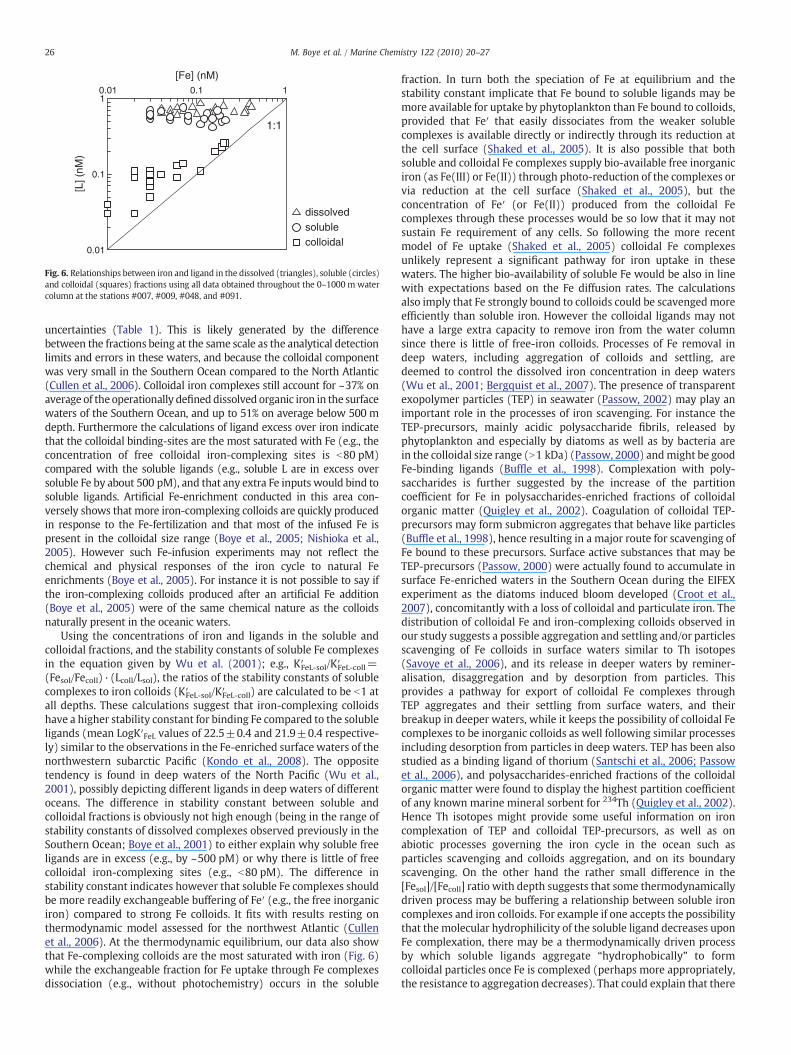
in excess over soluble Fe by ~0.5 nM on average (Table 1; Fig. 6), whilecolloidal L are comparatively almost saturated in colloidal Feproviding the relationship between the two parameters is linearwith a slope almost equal to 1 (e.g.; [Fecoll]=0.90 [Lcoll]−0.04 nM,r2=0.88, n=20; Fig. 6). The largest saturation of colloids with Fe andthe excess of soluble L over soluble Fe are obtained at the thermo-dynamic equilibrium in these waters. Hence it suggests that solubleligands have the potential to buffer an iron input to surface waterswhereas colloidal iron complexes may aggregate and settle.

Soluble Fe exists mainly as organic soluble complexes but it wasnot possible to discern whether iron colloids (e.g., the colloidal ironcomplexes) exist as organic complexes and/or inorganic amorphouscolloids from the data. Recent findings suggest that humic substances(HS) may account for a major portion of Fe complexation in seawaterand that a fraction of the Fe-HS species has a colloidal behavior(Laglera and van den Berg, 2009). It is hence conceivable that theextremely low concentration of free colloidal iron-complexing sites(e.g., 0–80 pM) is related to few complexation sites embedded withinan intricate architecture of very large molecular condensates. On theother hand inorganic Fe colloids can form surface active amorphouscolloids (Wells, 2003) that may appear as a (saturated) strong Fe-binding capacity upon titration (Boye et al., 2005), and/or provide alinear relationship between colloidal Fe and iron-complexing colloidswith a slope nearly equal to 1 like in this study. For instance

Soluble L<200 kDissolved L<0.2 µm (nM)

Dep

th (

m)

0.0 0.60.2 0.80.4 1.0 0.0 0.60.2 0.40

200

400

600

800

1000

Fig. 5. Vertical profiles of the iron binding ligand measured in the dissolved (b0.2 μm) and sofor stations #007 (49.29°S, 20.02°E), #009 (47.82°S, 20.79°E), #048 (48.59°S, 20.72°E), and

comparison between simple models of dissolved Fe equilibriumportioning and iron measurements in the dissolved and solublefractions suggested an inert colloidal fraction in the northwesternAtlantic that could be an iron oxide (Cullen et al., 2006). To assess suchpossibility we developed a model of iron portioning between solubleand colloidal fractions, resting on the relationship: FeL/Fe′=K′FeL⁎L′,which is obtained at the equilibrium of Fe′+L′←→FeL. In thisrelationship, FeL is the concentration of the organic iron, Fe′ theconcentration of inorganic iron, L′ the concentration of excess ligands(e.g., not bound to iron) and K′Fe′L the conditional stability constant ofFe–L complexes. Then the following Eq. (1) was obtained to predictthe ratio of Fesol/Fediss at the thermodynamic equilibrium, by using therelationship in the soluble and dissolved iron fractions, and byassuming Fe′sol≈Fe′diss (Fig. 6):

Fesol =Fedissð Þfrom model = 1 + L′solTK′FeL�solð Þ= 1 + L′dissTK′FeL�dissð Þ ð1Þ

The fraction of soluble iron predicted from the thermodynamicmodel (Fesol/Fediss frommodel) did not showhowever any significant trendwith the ratio calculated from the iron analyses (Fesol/Fediss measured) inthese waters (Table 1). Conversely, a systematically lower proportion ofsoluble iron was estimated from the model compared to the measure-ments in the North Atlantic (Cullen et al., 2006). The ratio estimatedfrom our model even displayed some values far above 1, with large

Da (nM)

St.007

St.009

St.048

St.091

Colloidal L>200 kDa-<0.2 µm (nM)

0.0 0.60.2 0.80.4 1.00.8 1.0

luble (b200 kDa) fractions, and calculated in the colloidal fraction (N200 kDa–b0.2 μm)#091 (48.17°S, 21.09°E) in the Southern Ocean.

1:1

[Fe] (nM)0.01 0.1 1

[L] (

nM)

0.01

0.1

1

dissolvedsolublecolloidal

Fig. 6. Relationships between iron and ligand in the dissolved (triangles), soluble (circles)and colloidal (squares) fractions using all data obtained throughout the 0–1000 m watercolumn at the stations #007, #009, #048, and #091.

26 M. Boye et al. / Marine Chemistry 122 (2010) 20–27

uncertainties (Table 1). This is likely generated by the differencebetween the fractions being at the same scale as the analytical detectionlimits and errors in these waters, and because the colloidal componentwas very small in the Southern Ocean compared to the North Atlantic(Cullen et al., 2006). Colloidal iron complexes still account for ~37% onaverage of the operationally defineddissolved organic iron in the surfacewaters of the Southern Ocean, and up to 51% on average below 500 mdepth. Furthermore the calculations of ligand excess over iron indicatethat the colloidal binding-sites are the most saturated with Fe (e.g., theconcentration of free colloidal iron-complexing sites is b80 pM)compared with the soluble ligands (e.g., soluble L are in excess oversoluble Fe by about 500 pM), and that any extra Fe inputs would bind tosoluble ligands. Artificial Fe-enrichment conducted in this area con-versely shows that more iron-complexing colloids are quickly producedin response to the Fe-fertilization and that most of the infused Fe ispresent in the colloidal size range (Boye et al., 2005; Nishioka et al.,2005). However such Fe-infusion experiments may not reflect thechemical and physical responses of the iron cycle to natural Feenrichments (Boye et al., 2005). For instance it is not possible to say ifthe iron-complexing colloids produced after an artificial Fe addition(Boye et al., 2005) were of the same chemical nature as the colloidsnaturally present in the oceanic waters.

Using the concentrations of iron and ligands in the soluble andcolloidal fractions, and the stability constants of soluble Fe complexesin the equation given by Wu et al. (2001); e.g., K′FeL-sol/K′FeL-coll=(Fesol/Fecoll)·(Lcoll/Lsol), the ratios of the stability constants of solublecomplexes to iron colloids (K′FeL-sol/K′FeL-coll) are calculated to be b1 atall depths. These calculations suggest that iron-complexing colloidshave a higher stability constant for binding Fe compared to the solubleligands (mean LogK′FeL values of 22.5±0.4 and 21.9±0.4 respective-ly) similar to the observations in the Fe-enriched surface waters of thenorthwestern subarctic Pacific (Kondo et al., 2008). The oppositetendency is found in deep waters of the North Pacific (Wu et al.,2001), possibly depicting different ligands in deep waters of differentoceans. The difference in stability constant between soluble andcolloidal fractions is obviously not high enough (being in the range ofstability constants of dissolved complexes observed previously in theSouthern Ocean; Boye et al., 2001) to either explain why soluble freeligands are in excess (e.g., by ~500 pM) or why there is little of freecolloidal iron-complexing sites (e.g., b80 pM). The difference instability constant indicates however that soluble Fe complexes shouldbe more readily exchangeable buffering of Fe′ (e.g., the free inorganiciron) compared to strong Fe colloids. It fits with results resting onthermodynamic model assessed for the northwest Atlantic (Cullenet al., 2006). At the thermodynamic equilibrium, our data also showthat Fe-complexing colloids are the most saturated with iron (Fig. 6)while the exchangeable fraction for Fe uptake through Fe complexesdissociation (e.g., without photochemistry) occurs in the soluble

fraction. In turn both the speciation of Fe at equilibrium and thestability constant implicate that Fe bound to soluble ligands may bemore available for uptake by phytoplankton than Fe bound to colloids,provided that Fe′ that easily dissociates from the weaker solublecomplexes is available directly or indirectly through its reduction atthe cell surface (Shaked et al., 2005). It is also possible that bothsoluble and colloidal Fe complexes supply bio-available free inorganiciron (as Fe(III) or Fe(II)) through photo-reduction of the complexes orvia reduction at the cell surface (Shaked et al., 2005), but theconcentration of Fe′ (or Fe(II)) produced from the colloidal Fecomplexes through these processes would be so low that it may notsustain Fe requirement of any cells. So following the more recentmodel of Fe uptake (Shaked et al., 2005) colloidal Fe complexesunlikely represent a significant pathway for iron uptake in thesewaters. The higher bio-availability of soluble Fe would be also in linewith expectations based on the Fe diffusion rates. The calculationsalso imply that Fe strongly bound to colloids could be scavengedmoreefficiently than soluble iron. However the colloidal ligands may nothave a large extra capacity to remove iron from the water columnsince there is little of free-iron colloids. Processes of Fe removal indeep waters, including aggregation of colloids and settling, aredeemed to control the dissolved iron concentration in deep waters(Wu et al., 2001; Bergquist et al., 2007). The presence of transparentexopolymer particles (TEP) in seawater (Passow, 2002) may play animportant role in the processes of iron scavenging. For instance theTEP-precursors, mainly acidic polysaccharide fibrils, released byphytoplankton and especially by diatoms as well as by bacteria arein the colloidal size range (N1 kDa) (Passow, 2000) andmight be goodFe-binding ligands (Buffle et al., 1998). Complexation with poly-saccharides is further suggested by the increase of the partitioncoefficient for Fe in polysaccharides-enriched fractions of colloidalorganic matter (Quigley et al., 2002). Coagulation of colloidal TEP-precursors may form submicron aggregates that behave like particles(Buffle et al., 1998), hence resulting in a major route for scavenging ofFe bound to these precursors. Surface active substances that may beTEP-precursors (Passow, 2000) were actually found to accumulate insurface Fe-enriched waters in the Southern Ocean during the EIFEXexperiment as the diatoms induced bloom developed (Croot et al.,2007), concomitantly with a loss of colloidal and particulate iron. Thedistribution of colloidal Fe and iron-complexing colloids observed inour study suggests a possible aggregation and settling and/or particlesscavenging of Fe colloids in surface waters similar to Th isotopes(Savoye et al., 2006), and its release in deeper waters by reminer-alisation, disaggregation and by desorption from particles. Thisprovides a pathway for export of colloidal Fe complexes throughTEP aggregates and their settling from surface waters, and theirbreakup in deeper waters, while it keeps the possibility of colloidal Fecomplexes to be inorganic colloids as well following similar processesincluding desorption from particles in deep waters. TEP has been alsostudied as a binding ligand of thorium (Santschi et al., 2006; Passowet al., 2006), and polysaccharides-enriched fractions of the colloidalorganic matter were found to display the highest partition coefficientof any known marine mineral sorbent for 234Th (Quigley et al., 2002).Hence Th isotopes might provide some useful information on ironcomplexation of TEP and colloidal TEP-precursors, as well as onabiotic processes governing the iron cycle in the ocean such asparticles scavenging and colloids aggregation, and on its boundaryscavenging. On the other hand the rather small difference in the[Fesol]/[Fecoll] ratio with depth suggests that some thermodynamicallydriven process may be buffering a relationship between soluble ironcomplexes and iron colloids. For example if one accepts the possibilitythat the molecular hydrophilicity of the soluble ligand decreases uponFe complexation, there may be a thermodynamically driven processby which soluble ligands aggregate “hydrophobically” to formcolloidal particles once Fe is complexed (perhaps more appropriately,the resistance to aggregation decreases). That could explain that there

27M. Boye et al. / Marine Chemistry 122 (2010) 20–27

is little of free colloidal Fe-complexing sites and it might provide anexplanation for the comparatively small difference in the partitioningof iron into colloidal particles with depth. However unlike microgels,any hydrophobically-driven aggregates would not disaggregate atdepth without there first being a loss of Fe from the complex, perhapsa difficult step; whereas aggregates may still be released fromremineralisation of larger particles. In turn the molecular nature ofiron colloids and the dynamics of the smaller fractions of dissolvediron clearly need to be further assessed. The role of soluble andcolloidal iron-species also needs to be further considered in models ofFe oceanic cycling.

Acknowledgements

The authors are most grateful for the assistance and logisticalsupport provided by the officers and crew of the R.V. Polarstern, as wellas chief scientist V. Smetacek (AWI, Germany), U. Bathmann (AWI,Germany), A.Watson (U. East Anglia, U.K.) andH. de Baar (Royal-NIOZ,The Netherlands) for their efforts in this expedition.We thank the twoanonymous referees whose remarks improved the manuscript. Thiswork was financed by the European Community projects CARUSO(ENV4-CT97-0472) and IRONAGES (EVK2-CT1999-00031).

References

Belkin, I.M., Gordon, A.L., 1996. Southern Ocean fronts from the Greenwich meridian toTasmania. Journal of Geophysical Research Oceans 101, 3675–3696.

Bergquist, B.A., Wu, J., Boyle, E.A., 2007. Variability in oceanic dissolved iron isdominated by the colloidal fraction. Geochimica et Cosmochimica Acta 71,2960–2974.

Boye, M., van den Berg, C.M.G., de Jong, J.T.M., Leach, H., Croot, P., de Baar, H.J.W., 2001.Organic complexation of iron in the Southern Ocean. Deep-Sea Research I 48,1477–1497.

Boye, M., Nishioka, J., Croot, P.L., Laan, P., Timmermans, K.R., de Baar, H.J.W., 2005. Majordeviations of iron complexation during 22 days of a mesoscale iron enrichment inthe open Southern Ocean. Marine Chemistry 96, 257–271.

Buffle, J., Wilkinson, K.J., Stoll, S., Filella, M., Zhang, J., 1998. A generalized description ofaquatic colloids interactions: the three-colloidal component approach. Environ-mental Science and Technology 32, 2887–2899.

Cisewski, B., Strass, V.H., Prandke, H., 2005. Upper-ocean vertical mixing in theAntarctic Polar Front Zone. Deep Sea Research II 52, 1087–1108.

Croot, P.L., Johansson, M., 2000. Determination of iron speciation by cathodic strippingvoltammetry in seawater using the competing ligand 2-(2-Thiazolylazo)-p-cresol(TAC). Electroanalysis 12 (8), 565–576.

Croot, P.L., Laan, P., Nishioka, J., Strass, V., Cisewski, B., Boye, M., Timmermans, K.R.,Bellerby, R.G., Goldson, L., Nightingale, P., de Baar, H.J.W., 2005. Spatial andtemporal distribution of Fe(II) and H2O2 during EisenEx, an open ocean mescoscaleiron enrichment. Marine Chemistry 95, 65–88.

Croot, P.L., Passow, U., Assmy, P., Jansen, S., Strass, V.H., 2007. Surface active substancesin the upper water column during a Southern Ocean Iron Fertilization Experiment(EIFEX). Geophysical Research Letters 34. doi:10.1029/2006GL028080.

Cullen, J.T., Bergquist, B.A., Moffett, J.W., 2006. Thermodynamic characterization of thepartitioning of iron between soluble and colloidal species in the Atlantic Ocean.Marine Chemistry 98, 295–303.

Gervais, F., Riebesell, U., Gorbunov, M.Y., 2002. Changes in primary productivity andchlorophyll-a in response to iron fertilization in the Southern Polar Frontal Zone.Limnology & Oceanography 47 (5), 1324–1335.

Gledhill, M., van den Berg, C.M.G., 1994. Determination of complexation of iron III withnatural organic complexing ligands in sea water using cathodic strippingvoltammetry. Marine Chemistry 47, 41–54.

Hartmann, C., Richter, K.-U., Harms, C., 2001. Distribution of nutrients during the Ironexperiment. Ber. Polarforsch. Meeresforsch., 400, Alfred-Wegener-Institut für Polarund Meeresforschung, Bremerhaven, Germany, pp. 186–190.

Hutchins, D.A., Witter, A.E., Butler, A., Luther III, G.W., 1999. Competition amongmarinephytoplankton for different chelated iron species. Nature 400, 858–861.

Johnson, K.S., Boyle, E., Bruland, K., Coale, K., Measures, C., Moffett, J., Aguilar-Islas, A.,Barbeau, K., Bergquist, B., Bowie, A., Buck, K., Cai, Y., Chase, Z., Cullen, J., Doi, Y.,Elrod, V., Fitzwater, S., Gordon, M., King, A., Laan, P., Laglera-Baquer, L., Landing, W.,Lohan, M., Mendez, J., Milne, A., Obata, H., Ossiander, L., Plant, J., Sarthou, G.,

Sedwick, P., Smith, G.J., Sohst, B., Tanner, S., van den Berg, C.M.G., Wu, J., 2007.Developing standards for dissolved iron in seawater. EOS 88 (11), 131–132.

Kattner, G., 2009. Nutrients measured on water bottle samples during POLARSTERN LegANT-XVIII/2. doi:10.1594/PANGAEA.713703.

Kondo, Y., Takeda, S., Nishioka, J., Obata, H., Furuya, K., Johnson, W.K., Wong, C.S., 2008.Organic iron(III) complexing ligands during an iron enrichment experiment in thewestern subarctic North Pacific. Geophysical Research Letters 35, L12601.doi:10.1029/2008GL033354.

Laglera, L.M., van den Berg, C.M.G., 2009. Evidence for the geochemical control of ironby humic substances in seawater. Limnology & Oceanography 54 (2), 610–619.

Nishioka, J., Takeda, S., Wong, C.S., 2001. Change in the concentrations of iron indifferent size fractions during a phytoplankton bloom in controlled ecosystemenclosures. Journal of Experimental Marine Biology and Ecology 258, 237–255.

Nishioka, J., Takeda, S., Kudo, I., Tsumune, D., Yoshimura, T., Kuma, K., Tsuda, A., 2003.Size-fractionated iron distributions and iron-limitation processes in the subarcticNW Pacific. Geophysical Research Letters 30 (14), 1730.

Nishioka, J., Takeda, S., de Baar, H.J.W., Croot, P.L., Boye, M., Laan, P., Timmermans, K.R.,2005. Changes in the concentration of iron in different size fractions during an ironenrichment experiment in the open Southern Ocean. Marine Chemistry 95, 51–63.

Obata, H., Karatani, H., Nakayama, E., 1993. Automated determination of iron inseawater by chelating resin concentration and chemiluminescence detection.Analytical Chemistry 65, 1524–1528.

Passow, U., 2000. Formation of Transparent Exopolymer Particles, TEP, from dissolvedprecursors material. Marine Ecology Progress Series 192, 1–11.

Passow, U., 2002. Transparent exopolymer particles (TEP) in aquatic environments.Progress in Oceanography 55, 287–333.

Passow, U., Dunne, J., Murray, J.W., Balistrieri, L., Alldredge, A.L., 2006. Organic carbon to234Th ratios of marine organic matter. Marine Chemistry 100, 323–336.

Quigley, M.S., Santschi, P.H., Hung, C.-C., Guo, L., Honeyman, B.D., 2002. Importance ofacid polysaccharides for 234Th complexation to marine organic matter. Limnologyand Oceanography 47, 367–377.

Riebesel, U., Gervais, F., Benthien, A., Terbrüggen, A., Schneider, A., Luz, B., Barkan, E.,Altabet, M., Saunders, R., 2001. Chlorophyll-a, particulate and dissolved organicmatter, primary production and stable isotope composition of POM andphytoplankton over the course of the iron fertilisation experiment. Ber. Polarforsch.Meeresforsch., 400, Alfred-Wegener-Institut für Polar und Meeresforschung,Bremerhaven, Germany, pp. 191–199.

Rue, E.L., Bruland, K.W., 1995. Complexation of iron (III) by natural organic ligands inthe Central North Pacific as determined by a new competitive ligand equilibration/adsorptive cathodic stripping voltammetric method. Marine Chemistry 50,117–138.

Ruzic, I., 1982. Theoretical aspects of the direct titration of natural waters and itsinformation yield for trace metal speciation. Analytica Chimica Acta 140, 99–113.

Santschi, P.H., Murray, J.W., Baskaran, M., Benitez-Nelson, C.R., Guo, L.D., Hung, C.-C.,Lamborg, C., Moran, S.B., Passow, U., Roy-Barman, M., 2006. Thorium speciation inseawater. Marine Chemistry 100, 250–268.

Savoye, N., Benitez-Nelson, C., Burd, A.B., Cochran, J.K., Charette, M., Buesseler, K.O.,Jackson, G.A., Roy-Barman, M., Schmidt, S., Elskens, M., 2006. 234Th sorption andexport models in the water column: a review. Marine Chemistry 100, 234–249.

Schlosser, C., Croot, P.L., 2008. Application of cross-flow filtration for determining thesolubility of iron species in open ocean seawater. Limnology & Oceanography:Methods 6, 630–642.

Shaked, Y., Kustka, A.B., Morel, F.M.M., 2005. A general model for iron acquisition byeukaryotic phytoplankton. Limnology and Oceanography 50, 872–882.

Strass, V.H., Leach, H., Cisewski, B., Gonzales, S., Post, J., da Silva Duarte, V., Trumm, F.,2001. The physical setting of the Southern Ocean iron fertilisation experiment.Ber. Polarforsch. Meeresforsch., 400, Alfred-Wegener-Institut für Polar undMeeresforschung, Bremerhaven, Germany, pp. 94–131.

Timmermans, K.R., van derWagt, B., de Baar, H.J.W., 2004. Growth rates, half-saturationconstants, and silicate, nitrate, and phosphate depletion in relation to ironavailability of four large, open-ocean diatoms from the Southern Ocean. Limnology& Oceanography 49 (6), 2141–2151.

van den Berg, C.M.G., 1995. Evidence for organic complexation of iron in seawater.Marine Chemistry 50, 139–157.

Wells, M.L., 2003. The level of iron enrichment required to initiate diatom blooms inHNLC waters. Marine Chemistry 82, 101–114.

Wells, M.L., Kozelka, P.B., Bruland, K.W., 1998. The complexation of ‘dissolved’ Cu, Zn,Cd and Pb by soluble and colloidal organic matter in Narragansett Bay. MarineChemistry 62, 203–217.

Wen, L.-S., Stordal, M.C., Tang, D., Gill, G.A., Santschi, P.H., 2000. An ultraclean cross-flowultrafiltration technique for the study of trace metal phase speciation in seawater.Marine Chemistry 55 (1–2), 129–152.

Wu, J.F., Luther III, G.W., 1995. Complexation of Fe(III) by natural organic ligands in theNorthwest Atlantic Ocean by competitive ligand equilibration method and a kineticapproach. Marine Chemistry 50, 159–178.

Wu, J.F., Boyle, E., Sunda, W., Wen, L.S., 2001. Soluble and colloidal iron in theoligotrophic North Atlantic and North Pacific. Science 293 (5531), 847–849.