Magnetocrystalline

in (FexNi1-x)

Anders StangelSupervisor: Jan

in (FexNi1-x)

FYSMAS1043

Examensarbete 30 hpAugusti 2016

Magnetocrystalline Anisotropy

)2B Materials

Anders StangelSupervisor: Jan Rusz

)2B Materials

Masterprogrammet i fysikMaster Programme in Physics

A

Magnetocrystalline Anisotropy in(FexNi1−x)2B Materials

The magnetic properties of the (FexNi1−x)2B family of materials are explored using DFT cal-

culations utilizing the FPLO and SPR-KKR code packages. It is found that a uniaxial magne-

tocrystalline anisotropy exists at around x = 0.8 with a magnetocrystalline anisotropy energy

at around 0.3MJm3 . A calculation of the lattice constant for these materials were attempted but

failed due to the emergence of local minima and the calculations of magnetic properties were

instead done using lattice parameters interpolated between known experimental values.

S

Permanentmagneter och magnetiska material har varit kända sedan antiken,då i form av naturliga permanentmagneter som till exempel magnetit. An-vändningsområdena då innefattade bland annat kompassen eller helt enkelsom en besynnerlig leksak. I modern tid har dock nya användningsområdenför magetiska material dykt upp, till exempel inom elekriska motorer, vind-kraftverk och hårddiskar. Dessa användningsområden har för med sig krav påkraftfullare magnetiska material än vad som behövts tidigare.

Flera exempel på kraftfulla permanent magneter existerar redan. De flestaav dessa använder sig av sällsynta jordartsmetaller som neodym och samar-ium. Sådana material har länga uppfyllt alla krav industrin har ställt på sinapermanentmagneter men de senaste åren har priset på dessa ämnen gått uppkraftigt vilket har skapat ett behov av material som uppfyller industrins kravpå prestanda utan att innehålla sällsynta jordartsmetaller.

Två av de egenskaper som är intressanta för en permanentmagnet är mag-netisk mättnad, som är ett mått på hur kraftfull magneten är, och koercivitetsom är ett mått på hur väl magneten står emot yttre magnetiska fält utan attdess magnetiska egenskaper försämras. Koerciviteten hos ett material kan isin tur räknas ut med hjälp av materialets magnetokristallina anisotropienergi(MAE) som är den mängd energi som behövs för att vrida det magnetiskafältet från sin naturliga riktning till den riktning som är svårast att uppnå förmaterialet. Denna egenskap har också fördelen att den kan säga oss någotom huruvida materialet är magnetisk i en specifik rikting alls eller om dennaturliga riktningen för det magnetiska fältet är utspritt över flera möjliga rik-tningar vilket skulle göra materialet oanvändbart som permanentmagnet.

I den här rapporten använder vi matematiska metoder för att räkna ut mag-netisk mättnad och MAE för en familj material bestående av bor förenat meden blandning av järn och nickel vilket ger den kemiska formeln (FexNi1−x)2B.Denna familj material har fördelen att alla beståndsdelar i materialet är billiga.Vi hittade ett område kring 80% järn där både den magnetiska mättnaden ochMAE är tillräckligt höga för att ämnena ska vara intressanta att studera när-mare.

!"#$

I would like to thank my supervisor Jan Rusz for his patient guidance throughthemaking of this work. In addition to him I want to thank Alexander Edström

and Mirosław Werwinski for their assistance in learning how to use the code

packages SPR-KKR and FPLO as well as giving invaluable input on the thesis

itself and my friends and family for all their love and support.

C%&'(&')

1 Introduction & Motivation . . . . . . . . . . . . . . . . . . . . . . . . . . . . . . . . . . . . . . . . . . . . . . . . . . . . . . . . . . . . . . . . . . . . . . . . . . 7

2 Theory . . . . . . . . . . . . . . . . . . . . . . . . . . . . . . . . . . . . . . . . . . . . . . . . . . . . . . . . . . . . . . . . . . . . . . . . . . . . . . . . . . . . . . . . . . . . . . . . . . . . . . . . . . 9

2.1 Theory of magnetism, relativistic electrons and spin-orbit

coupling . . . . . . . . . . . . . . . . . . . . . . . . . . . . . . . . . . . . . . . . . . . . . . . . . . . . . . . . . . . . . . . . . . . . . . . . . . . . . . . . . . . . . . . . . . . . 9

2.2 Magnetic anisotropy . . . . . . . . . . . . . . . . . . . . . . . . . . . . . . . . . . . . . . . . . . . . . . . . . . . . . . . . . . . . . . . . . . . . . . . 11

2.3 Density functional theory . . . . . . . . . . . . . . . . . . . . . . . . . . . . . . . . . . . . . . . . . . . . . . . . . . . . . . . . . . . . . 12

2.4 Treatment of randomly disordered alloys . . . . . . . . . . . . . . . . . . . . . . . . . . . . . . . . . . . . . 15

2.4.1 VCA . . . . . . . . . . . . . . . . . . . . . . . . . . . . . . . . . . . . . . . . . . . . . . . . . . . . . . . . . . . . . . . . . . . . . . . . . . . . . . . . . 16

2.4.2 CPA . . . . . . . . . . . . . . . . . . . . . . . . . . . . . . . . . . . . . . . . . . . . . . . . . . . . . . . . . . . . . . . . . . . . . . . . . . . . . . . . . . . 16

3 Computational Methods . . . . . . . . . . . . . . . . . . . . . . . . . . . . . . . . . . . . . . . . . . . . . . . . . . . . . . . . . . . . . . . . . . . . . . . . . . . . 19

3.1 SPR-KKR . . . . . . . . . . . . . . . . . . . . . . . . . . . . . . . . . . . . . . . . . . . . . . . . . . . . . . . . . . . . . . . . . . . . . . . . . . . . . . . . . . . . . . . 19

3.2 FPLO . . . . . . . . . . . . . . . . . . . . . . . . . . . . . . . . . . . . . . . . . . . . . . . . . . . . . . . . . . . . . . . . . . . . . . . . . . . . . . . . . . . . . . . . . . . . . . . 20

3.3 Calculating the Magnetocrystalline anisotropy energy and

magnetic moment . . . . . . . . . . . . . . . . . . . . . . . . . . . . . . . . . . . . . . . . . . . . . . . . . . . . . . . . . . . . . . . . . . . . . . . . . . . 21

3.4 DOS and bandstructure . . . . . . . . . . . . . . . . . . . . . . . . . . . . . . . . . . . . . . . . . . . . . . . . . . . . . . . . . . . . . . . . . . 22

4 Results . . . . . . . . . . . . . . . . . . . . . . . . . . . . . . . . . . . . . . . . . . . . . . . . . . . . . . . . . . . . . . . . . . . . . . . . . . . . . . . . . . . . . . . . . . . . . . . . . . . . . . . . 24

4.1 Lattice structure . . . . . . . . . . . . . . . . . . . . . . . . . . . . . . . . . . . . . . . . . . . . . . . . . . . . . . . . . . . . . . . . . . . . . . . . . . . . . . 24

4.2 Magnetic moment . . . . . . . . . . . . . . . . . . . . . . . . . . . . . . . . . . . . . . . . . . . . . . . . . . . . . . . . . . . . . . . . . . . . . . . . . . 25

4.3 MAE . . . . . . . . . . . . . . . . . . . . . . . . . . . . . . . . . . . . . . . . . . . . . . . . . . . . . . . . . . . . . . . . . . . . . . . . . . . . . . . . . . . . . . . . . . . . . . . . 26

4.4 DOS and bandstructure . . . . . . . . . . . . . . . . . . . . . . . . . . . . . . . . . . . . . . . . . . . . . . . . . . . . . . . . . . . . . . . . . . 27

5 Conclusion . . . . . . . . . . . . . . . . . . . . . . . . . . . . . . . . . . . . . . . . . . . . . . . . . . . . . . . . . . . . . . . . . . . . . . . . . . . . . . . . . . . . . . . . . . . . . . . . . 32

References . . . . . . . . . . . . . . . . . . . . . . . . . . . . . . . . . . . . . . . . . . . . . . . . . . . . . . . . . . . . . . . . . . . . . . . . . . . . . . . . . . . . . . . . . . . . . . . . . . . . . . . . 33

1* +,-./023-4/, 5 6/-478-4/,

The field of permanent magnet materials is one that has been extensively stud-

ied, both because of the complexities in the field and because of their applica-

tions in a wide number of fields ranging from electric motors, generators, tur-

bines, data storage devices, maglev transport and breaks in amusement parks

[1]. With these industries comes a demand for high-performance permanent

magnets. Several such high-performing permanent magnets already exist and

in particular magnets including rare-earth metals and transition metals have

shown to have magnetic properties superior to all known alternatives. The fact

that no other materials seemed to be able to compete with materials such as

SmCo5 and Nd2Fe14B long made these materials the primary options for in-

dustrial applications, having all the desired properties that the industry needed

out of a permanent magnet.

The price of the raw materials has proven to be another property that the

industry needs to take into account however and these rare-earth metals have

in recent years become less desirable for economic and political reasons [1,

2, 3, 4], and thus there is still a need for the development of new perma-

nentmagnetic materials, in particular materials that do not include rare-earth

metals. In searching for such a magnet the properties that need to be con-

sidered are the Curie temperature and the energy product, the latter of which

requires a large saturation magnetization and magnetocrystalline anisotropy

energy (MAE) to get coercivity. Several existing materials can already com-

pete with the strong rare-earth magnets for Curie temperatures and saturation

magnetization. These materials include the transition metals such as bcc Fe

and hcp Co. However, in these the MAE is lower by one or more orders of

magnitude compared to the rare-earth magnets. For bcc Fe this low MAE can

be explained by the inherent symmetry in the bcc structure where the magnetic

moments have many possible directions that are equivalent and the spin-orbit

coupling being main source of magnetic anisotropy is generally lower in high

symmetry crystals as long as perturbation theory holds. Other materials are

thus needed that fulfil the need for strong and stable permanent magnets made

from cheaper elements than the rare-earth metals. Materials with lower sym-

metry more easily lend themselves to magnetic anisotropy and higher spin

orbit coupling. One example of such symmetry breaking occurs in materials

with a tetragonal lattice structure rather than a cubic one like bcc Fe, since in

such a material, where the lattice constants fulfil c 6= a = b a magnetic mo-

ment along the z-axis and a magnetic moment along the plane orthogonal to

the z-axis is not symmetrically equivalent. Such a material could be of interest

7

p9:vided it shows easy axis magnetization rather than easy plane magnetiza-

tion.

A group of potential candidates stem from the family of materials based

on Fe2B which is known to have an tetragonal structure [5]. Fe2B has both

a high total magnetic moment per unit volume and a high MAE but the mag-

netic anisotropy is not uniaxial and is thus useless for applications. How-

ever, by alloying this material with other elements it has been shown to have

a uniaxial magnetic anisotropy. For example alloying Fe2B with cobalt to

become (FexCo1−x)2B does for certain values of x have both a uniaxial mag-

netic anisotropy and a sufficient MAE to make it interesting for further studies

[5, 6, 7, 8].

Another material that has been considered for alloying with Fe in Fe2B

is nickel. The alloy (FexNi1−x)2B has been shown [5] to have a tetragonal

structure for all values of x. Nickel serves as a complement to cobalt based

alloys because of the relative cheaper cost of nickel compared to cobalt. This

material does show lowmagnetic moment for high concentrations of nickel [5]

but may have uniaxial magnetic anisotropy for lower concentrations of nickel

and as such it is still a material of interest for study.

In this work the magnetization and MAE of (FexNi1−x)2B will be studied

for selected values of x using density functional theory (DFT), in order to de-

termine if the material for some concentration of Ni exhibits uniaxial magnetic

anisotropy and if so if the magnetization and MAE is large enough for indus-

trial applications. The density of states and bandstructure of selected values of

x is presented as a framework to discuss the nature of this family of materials.

The theory of magnetism will be discussed in chapter 2 to the extent relevant

for this study. In chapter 3 an overview of the specific computational methods

used in the study will be presented and finally in chapters 4 and 5 the results

of the study will be presented and discussed respectively, in addition to a brief

discussion on potential future studies based on the findings.

8

;< =>?@BD

Here the relevant theory and mathematical background is presented. The

theory of magnetism with spin-orbit coupling and the arising of magnetic

anisotropy is presented and finally the mathematical treatment and relevant

approximations of DFT and the approximations used to treat random alloying

are outlined.

2.1 Theory of magnetism, relativistic electrons and

spin-orbit coupling

The spontaneous magnetic field of a material arises due to the spin and the or-

bital angular momentum of the material’s electrons, each of the quantum num-

bers providing a contribution to the total magnetic moment. The Schrödinger

equation of a wave function Ψ

HΨ(x) = EΨ(x), (2.1)

where H is the Hamiltonian operator gives a non-relativistic description of the

electrons in a system. In the early days of quantum mechanics experiments

showed that the electrons had twice the expected number of allowed states. To

solve this, spin was introduced to account for these extra states [9, 10]. While

trying to work out relativistic quantum mechanics Dirac [11, 12] introduced

the relativistic equation

[

i∂

∂ t+ eA0+ γ1

(

i∂

∂x1+ eA1

)

+ γ2

(

i∂

∂x2+ eA2

)

+γ3

(

i∂

∂x3+ eA3

)

+ γ0m

]

ψ = 0

(2.2)

in natural units or written in another way

(

γµ(

i∂µ − eAµ

)

−m)

ψ = 0. (2.3)

Aµ here are arbitrary electromagnetic fields of potential, γµ are the Dirac ma-

trices and e and m are the electron charge and mass respectively. From here

the spin appeared as an internal angular momentum in addition to the orbital

angular momentum in order to preserve Lorenz invariance. Equation 2.3 does

9

aEEFGaHIJK LIMEGNOI MPNQRTGONH ETFPJNQU V13] giving rise to the effective mag-

netic magnetocrystalline anisotropy . Equation 2.3 can after separating out

time independence be written as the Kohn-Sham-Dirac equations [14]

[

−iα∇+βm+Aeff− εi

]

φi (r) = 0 (2.4)

where Aeff is the effective magnetic vector potential, φi (r) are the eigenfunc-tions of the Kohn-Sham equations described further in section 2.3 and α and

β are the Dirac matrices. Aeff can then be given as a functional of exchange

and correlation energies [14].

Aeff =−(

V ext (r)+ e2∫

n(r′)|r− r′|dr′+

δERxc

δn(r)

)

I

−eα

(

Aext (r)+ e

∫

J (r′)dr′

|r− r′| +δER

xc

δJ (r)

)(2.5)

Note the similarities between equations 2.5 and the potential terms in equa-

tions 2.17 and 2.21. This functional appearance of the potentials will be fur-

ther discussed in section 2.3.

This formalism treats the spin-orbit coupling and the scattering spin polar-

ization on equal footing. Depending on the material it is possible to get the

same accuracy with less computation power by treating one of them variation-

ally or as a perturbation to a scalar relativistic approximation that otherwise

would lack a spin-orbit coupling term [15] where the added a spin-orbit cou-

pling term becomes [16]

HSOC =c2

(2c2−V )2σ · (∇V ×p) , (2.6)

which can be taken along with other relativistic effects such as the mass-

velocity enhancement [17]

Hmv =−p4

8m3c2(2.7)

and the Darwin term [18].

HDarwin =e∇2V

8c2m2(2.8)

In this work fully relativistic calculations will be performed for of all elec-

tronic state and magnetization calculations.

10

WXW Magnetic anisotropy

Magnetic anisotropy is the directional energy dependence of the magnetic mo-

ment in a material in the absence of an external magnetic field. This directional

dependence is determined by a vast number of factors including morphology,

chemical composition, alloying order of the material in addition to any sur-

face, interface or impurities. In this work, a perfect crystal without impuri-

ties, surfaces and interfaces is assumed and these effects are thus not taken

into consideration. While many different kinds of magnetic anisotropy exists

[19] the two most discussed kinds are magnetocrystalline anisotropy and shape

anisotropy. In this work the focus will be on magnetocrystalline anisotropy.

The magnetic anisotropy is often expressed in terms of the anisotropy con-

stants Ki for i= 1,2,3, · · · so that magnetic anisotropy can be expressed as

E = Eiso+∑i

ciKi, (2.9)

where ci depends on the direction of the magnetic moments and Eiso is the part

of the energy that is not directionally dependent. For example in a uniaxial

crystal the magnetic anisotropy can be expressed as

E = Eiso+K1 sin2 (θ)+K2 sin

4 (θ)+K3 sin6 (θ)cos(6φ)+ · · · , (2.10)

where θ is the angle between the magnetization and the z-axis and φ is the

azimuthal angle to the z-axis[3] and for a cubic crystal the magnetic anisotropy

can be expressed as

E =Eiso+K1

(

α21α2

2 +α22α2

3 +α23α2

1

)

+K2α21α2

2α23+K3

(

α21α2

2 +α22α2

3 +α23α2

1

)2 · · ·(2.11)

where αi is the cosine of the angle with respect to the cubic axes. Both the

anisotropy constants and the general structure of the magnetic anisotropy is

thus obviously material dependent [20].

In this work materials with a uniaxial crystal structure will be studied so

equation 2.10 would describe the magnetic anisotropy of this material if the

values of Ki where known for all values of i = 1,2,3, · · · . For the purposes

of this work the magnetic anisotropy arises as a result of spin-orbit coupling

outlined in section 2.1. The spin-orbit coupling however is a relativistic effect

and needs to be more carefully treated [21, 22].

The MAE is then tied to the magnetic anisotropy stemming from the energy

calculated for example in equation 2.10 or 2.11. The MAE is defined as the

maximal difference in energy over the magnetization directions.

EMAE = E (θ ,φ)max−E (θ ,φ)min (2.12)

Note that the isotropic part Eiso always disappear in such an equation due to

it being the same in both terms. As such the MAE is a measurement of the

11

sYZ[\]\Y^ _` Ybc dZefcY\gZY\_f h\icjY\_f \f Z dZYci\Z] k\Yb Z b\eb lmn [c\feneeded for a good permanent magnet.

2.3 Density functional theory

All of the preceding is based on the interactions between a large number of

electrons. This is dealt with in part by realizing that the system is a periodic

infinite crystal and as such it can efficiently be treated through a Fourier trans-

form. In the explicit method of summing up the interaction between every pair

of electrons and ions the Hamiltonian would represent the total energy of the

system from all those contributions of a system withM ions and N electrons

H =−1

2

N

∑i=1

∇2i −

1

2

M

∑A=1

1

MA

∇2A−

N

∑i=1

M

∑A=1

ZA

riA+

N

∑i=1

N

∑j>i

1

ri j+

M

∑A=1

M

∑B>A

ZAZB

RAB

(2.13)

whereMA and ZA is the mass and atomic number of ion A and e= 1[23]. Deal-

ing with these interactions between each electron pair separately and coupling

the electrons and ions will prove to be too computationally heavy for any large

system. One method that has been proven to be a powerful tool in calculating

the ground state of materials is density functional theory (DFT).

DFT is an ab initio theory of matter and as such derives all its results from

first principles without additional assumptions, having its roots in established

quantum mechanics [23]. It starts from the non-relativistic Schrödinger equa-

tion representing the wave function Ψ in equation 2.1. The kinetic term from

the ions in equation 2.13 disappears under the Born-Oppenheimer approxi-

mation but since the calculations still scale with the number of atoms in the

system it is still clear that this yields unfeasibly large calculations for large

systems. In addition to that, the electrons in a magnetic system cannot be

treated as non-relativistic as explained in section 2.1. A reasonable attempt

would be to try and generalize the many-body problem for the non relativistic

case in such a way that it can be extended into the relativistic case.

The Hamiltonian in equation 2.13 can be rewritten with the different types

of interaction specified.

H =

(

− h2

2m

N

∑i=1

∇2i +

N

∑i

Vext (ri)+1

2

N

∑i6= j

w(|ri− r j|))

(2.14)

where Vext(r) is the external potential, which in equation 2.13 corresponds to

the interactions with the ions, and w(|ri− r j|) is the Coulomb interaction be-

tween two electrons at sites i and j. While equation 2.14 removes the need

to sum up the ions for any other purpose than to determine Vext(r) it still re-quires explicit summation over the electrons. This problem has been treated in

12

oqrferent ways, including the Hartree-Fock theory that treated the many body

problem as a set of equations with a Slater determinant of one particle wave

functions [24]. The Hartree-Fock theory could not account for correlation ef-

fects in the system however [25] and other methods became necessary. DFT

got its foundation in the first Hohenberg-Kohn theorem which showed that

the total energy ground state could be uniquely determined from the electron

density [26, 23] And that the energy could be written as a functional of the

electron density in a static potential v

E [n] =∫

Vext(r)n(r)dr+1

2

∫ ∫

n(r)n(r′)|r− r′| drdr′+G[n], (2.15)

where n is the electron density andG[n] is a universal functional of the electrondensity [26]. The correlation effects missing from the Hartree-Fock theory

show up in equation 2.15 in the univeral functional G[n]

G[n]≡ Ts[n]+Exc[n]. (2.16)

Ts here is the kinetic energy functional and Exc[n] is the exchange-correlationfunctional which can in turn be divided into an exchange and a correlation

part [25]. The Hohenberg-Kohn theorem allows the system to be reduced

from a many-body problem to a single particle problem using the Kohn-Sham

approach where the system is set up as a system of equations.

[

−1

2∇2+Vext (r)+

∫

n(r′)|r− r′|dr′+

δ (nεxc (n))

δn

]

ψi (r) = εiψi (r) , (2.17)

for a local potential [25]. Here εxc is the exchange-correlation energy per

particle in the system. Equation 2.17 has a kinetic term and several potential

terms including the external potential that can be expressed as an effective

potential of the system.

Veff =Vext (r)+∫

n(r′)|r− r′|dr′+

δ (nεxc (n))

δn(2.18)

Of these terms Vext is assumed to be known from the system and∫ n(r′)|r−r′|dr′

is a known quantity as long as n(r) is known. n(r) can be calculated using

a starting guess and then using an iterative process until self-consistency is

achieved. Methods for this are discussed in section 3.1 and 3.2. The only

unknown term thus stems from the exchange correlation potential.

Vxc =δ (nεxc (n))

δn, (2.19)

13

wtuvt ux y zy|u~ ty |x y xyy~ ty t |state electron density in this system can be expressed by the Kohn-Sham or-

bitals themselves.

n(r) =N

∑i=1

|ψi (r)|2 (2.20)

where the sum is over the N lowest energy states. The many-body problem of

several electrons has thus been reduced to a single body problem with several

eigenstates.

This approach so far has assumed a local external potential. It is possible

to extend the Hohenberg-Kohn theorem to non-local potentials as well [27]

without the loss of universality in the energy functionals and this non-locality

has to be treated separately. Here the potential Vxc and thus the functional that

describes it can be divided into an exchange part and a correlation part so that

(

−1

2∇2+Vext(r)+

∫

n(r′)|r− r′|dr′+

δ (nεc (n))

δn

)

ψi−∫

n1(r,r′)

|r− r′| ψi(r′)dr′= εiψi(r),

(2.21)

where εc is the correlation energy per particle in the system and n1 is the

overlap between wave-functions at different sites [25].

n1(

r,r′)

=N

∑i=1

ψ (r)ψ∗(

r′)

(2.22)

As can be seen from equations 2.21 and 2.22 this approach does not add any

new unknown quantities to the system, though it changes Vxc to Vc. Provided

that these quantities can be known exactly this approach would yield an exact

result.

In practice however this is not the case apart from a few rare exceptions and

approximations need to be done. The most basic of these approximations is

the local density approximation (LDA) where the exchange-correlation func-

tional Exc is expressed purely in terms of the density itself, treating Exc like in a

homogenous electron gas in every point [28]. This approximation can also be

expanded to differ between the density of electrons with spin up and electron

with spin down where n(r) = n(r)↑+n(r)↓ leading to the local spin-density

approximation (LSDA). Collectively these two approximations are known as

the local (spin-) density approximation (L(S)DA) when discussing properties

that the two approximations have in common. L(S)DA has shown to give ac-

ceptable results for calculations of molecular geometries and frequencies but

lacks in calculations of binding energies since it tends to lead to overbinding

in addition to miscalculating the exchange energy [28, 29] as well as underes-

timating the band gap in semiconductors and insulators [30]. One correction

is to add the terms from the Coulomb interactions and exchange interactions

14

¡ ¢£ ¡provides an improvement over L(S)DA for strongly correlated systems such

as can be found with rare-earth metal ions with partially filled f-shells or tran-

sition metals with partially filled d-shells [31]. Another approximation that

has shown to be superior to L(S)DA for strongly correlated systems is the dy-

namic mean-field theory (DMFT) that changes the static mean field potential

of previously mentioned DFT approximations for a dynamic potential [32].

Typically DMFT is used in a hybrid functional combining DMFT with LDA

or another approximation [32, 33].

The generalized gradient approximation (GGA) takes LDA one step fur-

ther by incorporating the gradients of the electron density in addition to the

electron density itself. It is known to provide an overall improvement over

LDA for many systems and properties though it can be found to slightly over-

estimate lattice constants [34]. In order to calculate magnetic properties of

materials GGA too needs to go to spin-polarized DFT as was done going from

LDA to LSDA with appropriate changes to the effective potential in equation

2.18. This has been shown to give calculations of satisfactory accuracy for

calculations of magnetic properties of transition metals [35].

In this work the GGA model by Perdew, Burke and Ernzerhof (PBE) will

be used since that has been shown to have a good accuracy for treatment of

magnetic properties of 3d transition metals and compounds of 3d transition

metals[36].

2.4 Treatment of randomly disordered alloys

Having a fundamental framework for dealing with many body systems such as

solid matter including the particular material of interest here the only thing left

is to deal with the alloying of the material. For a (FexNi1−x)2B crystal where

x 6= 0 and x 6= 1 the random instances of iron or nickel need to be treated. One

way of treating the system is, by instead of doing calculations on small repeat-

ing unit cells, use the supercell approximation in which a supercell consisting

of several unit cells with one or more disordered configuration with imposed

periodic boundary conditions is taken as the periodic unit cell. In order to ac-

quire accurate results with such a system many configurations would generally

have to be considered [37] and while the supercell approximation would ac-

curately describe the system for a large enough super cell it would thus prove

to be computationally too heavy since it demands that a much larger space be

considered explicitly. Some other approximation is thus needed to get viable

computation methods. Here two such approximations will be considered.

15

¤¥¦¥§ VCA

The first approximation is the virtual crystal approximation (VCA). In VCA

the alloyed sites are considered to be virtual atoms of the same species with

an atomic number that is the average of the two alloyed species weighted de-

pending on the value of x. So for an alloy with the proportions X = AxB1−x inthe VCA the alloy sites gets a single potential that is taken to be the average

of the potentials from the alloyed elements, creating a virtual element at that

site with potential [37]

VVirtual = xVA+(1−x)VB, (2.23)

and the virtual element is thus taken to have atomic number ZVirtual = xZA+(1−x)ZB. The non alloyed elements of the crystal can then take its normal

potential giving a crystal such as (FexNi1−x)2B in the calculation becomes

X2B where X is the virtual element put in place by the VCA.

The premise for this approximation is simple and its implementation is sim-

ple [38] and efficient [37]. Still the model is known to produce results of good

accuracy for yielding wave functions and energy spectra in alloys [39] and spin

and orbital moments [38, 40]. The nature of VCA does imply that the approx-

imation is better for alloying elements which are neighbouring each other on

the periodic table, such as alloying Fe and Co or Co and Ni [38], while giving

a less accurate result for elements that are further apart in the periodic table,

such as Fe and Ni. For the calculations needed for this study, VCA has shown

to vastly overestimate the MAE of systems, though the MAE as a function of

alloy concentration in an alloy can be expected to have qualitatively the right

shape [40].

This work does utilize VCA to treat a disordered alloy of Fe and Ni and

calculating the MAE using it with the FPLO method described in section 3.2

in spite of these well documented shortcomings. The MAE from these calcu-

lations are expected to be vastly overestimated, though the shape of the MAE

as a function of alloy concentration is expected to be correct. It can thus be

used to check for errors while using other methods like the SPR-KKR method

described in section 3.1 which instead of VCA utilizes the coherent potential

approximation (CPA) described in subsection 2.4.2. In addition to that, since

the total energy as a function of the lattice parameters a and c is expected to be

conceptually correct [41], FPLO can be utilized to perform lattice relaxation

calculations where the exact total energy is less important than the values of

the lattice parameters where the energy function has a minimum.

2.4.2 CPA

The second approximation that will be considered is the coherent potential

approximation (CPA). In CPA the disorder is treated by adding impurities of

the alloyed materials in an effective CPA medium [42] with the condition that

16

¨© ª«¬­ª®¬ ©¨ ¯°ª±±¬­²©® ¨°°³­¯ ´¨­ ª ¯²©®µ¬ ¬µ¬°±­¨© ±­ª«¬µµ²©® ²© ±¶¬ ·¸¹medium when a single CPA scattering matrix gets replaced with an atom spe-

cific scattering matrix of one of the alloyed types [43].

CPA is based on a Green’s function approach [42]. A Green’s function

G(x,x′) to an operator f (x) fulfills

f (x)G(

x,x′)

= δ(

x−x′)

, (2.24)

where δ (x−x′) is the Dirac delta. Here the Green’s function in question is

the Green’s function to the Hamiltonian.

(

E− H)

G(

r,r′;E)

= δ(

r− r′)

(2.25)

The Green’s function of such a system is a powerful tool in electronic structure

theory by defining the electron density [44, 45].

n(r) =− 1

π

EF∫

−∞

IG(r,r;E)dE (2.26)

Naturally the Green’s function depends on the elements involved in the alloy

and their concentrations since it’s defined by the Hamiltonian. The Green’s

function is the response function of the system [46] and is thus used in the

t-matrix scattering approximation [47] defined by an implicit equation for an

atom type α [42].

tα (E) = vα + vαG0 (E) tα (E) , (2.27)

where vα is the perturbation potential for the atom type α and G0 is the free

electron Green’s function. This total scattering matrix can be expressed in

terms of the scattering path operators which includes all possible scattering

events between cells n and m [47].

t (E) = ∑nm

τnm (E) (2.28)

A binary disordered alloy such as the alloy of Fe and Ni considered in this

work has only site-diagonal elements considered in the disorder [48], and thus

the only elements of the single site scattering operators are the case when

m = n which in terms of the scattering path operator can be expressed as a

sum of the off-diagonal elements [45]

tnn (E) = ∑i 6=n

∑j 6=n

τi j (E) . (2.29)

An effective CPA medium can then be taken to be a potential v0 that has yet

to be defined. All potentials belonging to the actual atoms can then be taken

to be some perturbation to this CPA medium vα = vi− v0 where i is the atom

17

º»¼½ and the unperturbed Green’s function of the pure CPA medium system G

can thus be defined through a Dyson equation [42].

G0 = G0+G0

(

∫

v0 (x)dx

)

G0 (2.30)

with G0 defined as before. The CPA medium scattering operator t can then be

defined with the perturbations vα

tα (E) = (vi− v0)+(vi− v0) G0 (E) tα (E) , (2.31)

and a CPA t matrix is obtained from the unperturbed system.

tCPA (E) = v0+ v0G0 (E) tCPA (E) (2.32)

So far, as long as v0 and vi are chosen correctly this is all exact. The approx-

imation is then to assume that the paths are sufficiently long so that the concept

of an average medium should provide a close enough approximation to the av-

erage path taken in the actual crystal [42]. The CPA scattering medium is then

the weighted average of the scattering media of the pure crystals of respective

alloying species [49].

τCPAnn = ∑α

cαταnn, (2.33)

where cα is the concentration of element α and

(ταnn)

−1 = (tαnn)−1−

(

tCPAnn

)−1−(

τCPA)−1

. (2.34)

From equations 2.33 and 2.34 CPA averaged Green’s function can thus be

obtained.

GCPA(

r,r′,E)

= ∑α

cαGα(

r,r′,E)

(2.35)

CPA is a more sophisticated approach than VCA and it gives a more ac-

curate estimate of the MAE. While this CPA method fails in accounting for

environmental effects or other such non-local effects except as an average [50]

it can be expected to be accurate enough for all the electronic structure calcu-

lations considered in this work [39, 40, 51]. This work utilizes CPA within the

SPR-KKR code package described in section 3.1.

18

¾¿ ÀÁÂÃÄÅÆÅÇÁÈÆÉ ÊËÅÌÁÍÎ

Here the computational methods will be discussed. First the code packages

SPR-KKR and FPLO will be presented together with a brief outline of the

underlying method. Then a theoretical background in methods to specifically

calculate the MAE, DOS and band structure will be given.

3.1 SPR-KKR

The Spin Polarized Relativistic Korringa-Kohn-Rostocker method (SPR-KKR)

is based on the works by Korringa [52], Kohn and Rostoker [53], also known

as multiple scattering theory. The method utilizes the Green’s functions of

equation 2.25. The method utilizes the t matrix and scattering path operators

outlined in 2.4.2 finding the scattering path operator as [54]

τnm (E) =(

t (E)−1−g(E))−1

nm(3.1)

for an electron at cite n with a scattering path to cite m and where g(E) in-cludes the structure constants of the system [47]. These can be retrieved

through the unperturbed Green’s function

G0 (r,r;E) =−ip∑L

jl (pr<)h+l (pr>)YL (r)Y

∗L

(

r′)

(3.2)

where p=√E, jl (z) and h

+l (z) are the spherical Bessel and Hankel functions

respectively and YL are spherical harmonics by using the scattering operator

T (E) and that can be retrieved from

T (E) =V (r)+V (r)G0 (E)T (E) (3.3)

where V (r) is the potential of the system and the scattering operator is con-

nected to the scattering path operator through [47]

T (E) = ∑nm

τnm (E) (3.4)

From equation 3.1 the scattering path operator can be used to calculate the

Green’s function through [49]

19

Ï(

r,r′;E)

= ∑ΛΛ′

ZnΛ (r,E)τnn

′ΛΛ′ (E)Z

n′×Λ′(

r′,E)

−∑Λ

(

ZnΛ (r,E)J

n×Λ

(

r′,E)

Θ(

r′− r)

+JnΛ (r,E)Zn×Λ

(

r′,E)

Θ(

r− r′))

δnn′ .

(3.5)

where ZnΛ (r,E) and JnΛ (r

′,E) are the regular and irregular solutions to the

radial Schrödinger equaion. Using the Green’s function the charge density

is obtained from equation 2.26 and it is possible to calculate the dispersion

relation E (k) as well as the spin magnetic moment

µspin =−µB

πℑTr

∫ EFdE

∫

Vd3rβσzG

(

r,r′;E)

(3.6)

and orbital magnetic moment

µorb =−µB

πℑTr

∫ EFdE

∫

Vd3rβ lzG

(

r,r′;E)

(3.7)

where β = γ0 is the Dirac matrix of index zero, σz is the third Pauli matrix and

lz is the orbital angular momentum matrix.

This method lends itself well to the CPA approach described in section 2.4.2

by transforming the scattering path operator in equation 3.1 using the CPA

equations given in equations 2.33 and 2.34 and then using the CPA medium

to calculate a new Green’s function from equation 2.35. The above formalism

can then be utilized with the new Green’s function as normal.

3.2 FPLO

The full potential local orbital (FPLO) method uses a real space representation

of non-orthogonal local orbitals. The potential v(r) can be represented as

v(r) = ∑R+s,L

vs,L|r−R− s|YL (r−R− s) , (3.8)

where R is the Bravais lattice vector, s is a basis vector for the unit cell and YLare the real spherical harmonics of orbital L to solve the Kohn-Sham equations

and describe the density and potential while solving the Hartree potential using

the Poisson equation [41] leaving only the exchange and correlation potential

to be solved separately by decomposing them into parts centred at the lattice

sites and vanishing quickly when approaching neighbouring sites [55]. This is

accomplished by partitioning utilizing a shape function defined such that

∑R+s

fs (r−R− s)≡ 1 (3.9)

20

ÐÑÒ ÑÓÔÕÐÖ×ØÙÒ ÐÚÚÓÔÒ×ÑÛ ÜÓ

fs (r) =∏τH (−r)

(

τr

|τ|2)

∑τ

∏τH (τ− r)

(

τ(r−τ)

|τ|2) (3.10)

where H (x) is the Heaviside step function and τ = R− s′− s is a vector point-

ing to any point from the centre of a cell.

The Kohn-Sham equations are solved using the ansatz of the superposition

of Bloch-states

|kn〉= |RsL〉cknLse

ik(R+s) (3.11)

The high localization of orbitals allows for splitting of valence and core or-

bitals where the core orbitals are so localized that the spherical average can be

used in place of equation 3.8,

⟨

R′s′L′c|RsLc⟩

= δL′cLcδR′+s′,R+s, (3.12)

where Lc are the core orbitals. The on-site electron density can then be calcu-

lated as a sum of the overlap densities from core orbitals, valence orbitals and

the combination thereof [41].

n=occ

∑kn

= |kn〉〈kn| (3.13)

non−siteRs = non−site,ccRs +n

on−site,cvRs +n

on−site,vvRs (3.14)

where vv refers to overlap between valence orbitals and so on. In this work

the FPLO method will be used in combination with VCA described in section

2.4.1 to treat disorder.

3.3 Calculating the Magnetocrystalline anisotropy

energy and magnetic moment

In section 2.2, the magnetic anisotropy was discussed. Here the practical

computations of the magnetic moment and the MAE will be presented.

The calculations of the magnetic moment is generally fairly straight forward

since it falls out from spin polarized calculation of the electron density as

n(r) = n↑ (r)+n↓ (r) . (3.15)

In the SPR-KKR method described in section 3.1 this relation falls out into

equations 3.6 and 3.7. In the case of the FPLO method described in section

21

ÝÞß the magnetic moment is calculated directly from the SCF calculation of

the electron density.

The MAE can be calculated as the maximum between two magnetization

directions.

|EMAE|= |E (n1)−E (n2)|= |Emin−Emax| , (3.16)

where n1 is the preferred direction for the magnetization so that E (n1) =Emaxand n2 is the magnetization direction with the lowest energy. E (n2) =Emin. n1 is called the easy axis and n2 is called the hard axis. The sign for

the MAE is decided according to some convention. One problem with this

method for a general crystal is how to find the easy and the hard axes and thus

the maximum and the minimum values for the MAE. This tends not to be a

problem in practice since the preferred axis often is along a high symmetry

axis in the crystal. In a uniaxial crystal for example the crystal generally has

uniaxial magnetization with the easy axis being along the z-axis and the hard

axis along the plane orthogonal to the z-axis or vice versa.

As long as n1 and n2 are the correct choices for the easy and the hard axes

the total energy difference method will yield correct results by definition of

EMAE. Some care needs to be taken with the method since EMAE tends to be

very small compared to the value of Emin and Emax.

3.4 DOS and bandstructure

Quantum mechanics gives us the result that an electron in a material system

cannot have any arbitrary energy. Instead it is confined to allowed energy

levels. In a solid crystal these allowed states depend on the crystal momentum

giving rise to a bandstructure.

The bandstructure of a material is the allowed energy levels as a function

of crystal momentum. This is most notably expressed by finding the energy

dispersion relation E (k). In this work however the main focus will be on

disordered alloys and the energy dispersion relation is replaced by the Bloch

spectral function A(k,E) which reduces to the energy dispersion relation in

the ordered limit. The Bloch spectral function can be expressed like a Fourier

transform of the Green’s function [21]

A(k,E) =− 1

πNℑTr

N

∑n,n′

eik(Rn−Rn′)×∫

ΩG(r+Rn,r+Rn′ ,E)d

3r (3.17)

The density of states (DOS) of a material is a measure of howmany electron

states is allowed per energy step in a crystal as a function of energy. The

density of states is tied to the electron density n(ε) through [56]

22

à=∫

Vg(ε) f (ε)dε (3.18)

where g(ε) is the density of states at energy ε , V is the volume of a primitive

cell and f (ε) is the Fermi function.

Equations 3.18 requires finite temperatures however and a way to define

this function in the ground state is needed. In a Green’s function method

like SPR-KKR described in section 3.1 the density of states can be calculated

using its ties to the Green’s function described in section 2.4.2. Since the elec-

tron density can be calculated directly from the imaginary part of the Green’s

function using equations 2.26 and 3.18 the imaginary part of the Green’s func-

tion G(r,r,E) can be seen as a local density of states at site r [57]. From the

equations 3.18 and 2.26 it can be seen that the imaginary part of the Green’s

function is tied to the density of states through the identity [58]

g(E) =− 1

πℑTrG0 (E) (3.19)

for a system of non-interacting electrons and to add interaction add the inter-

acting Green’s function.

δg(E) =− 1

πℑTr(G0 (E)−G(E)) (3.20)

This Lloyd’s formula can be used to find the density of state [21, 58, 59]. Uti-

lizing these methods to calculate the scattering matrices and Green’s function,

the density of states is obtained.

23

áâ ãäåæçèå

Here the results of the study are presented. First the lattice constants, total

magnetic moments and the MAE of the materials as a function of alloying

concentration is plotted. Finally some DOS and band-plots of selected values

of the alloying concentration are presented.

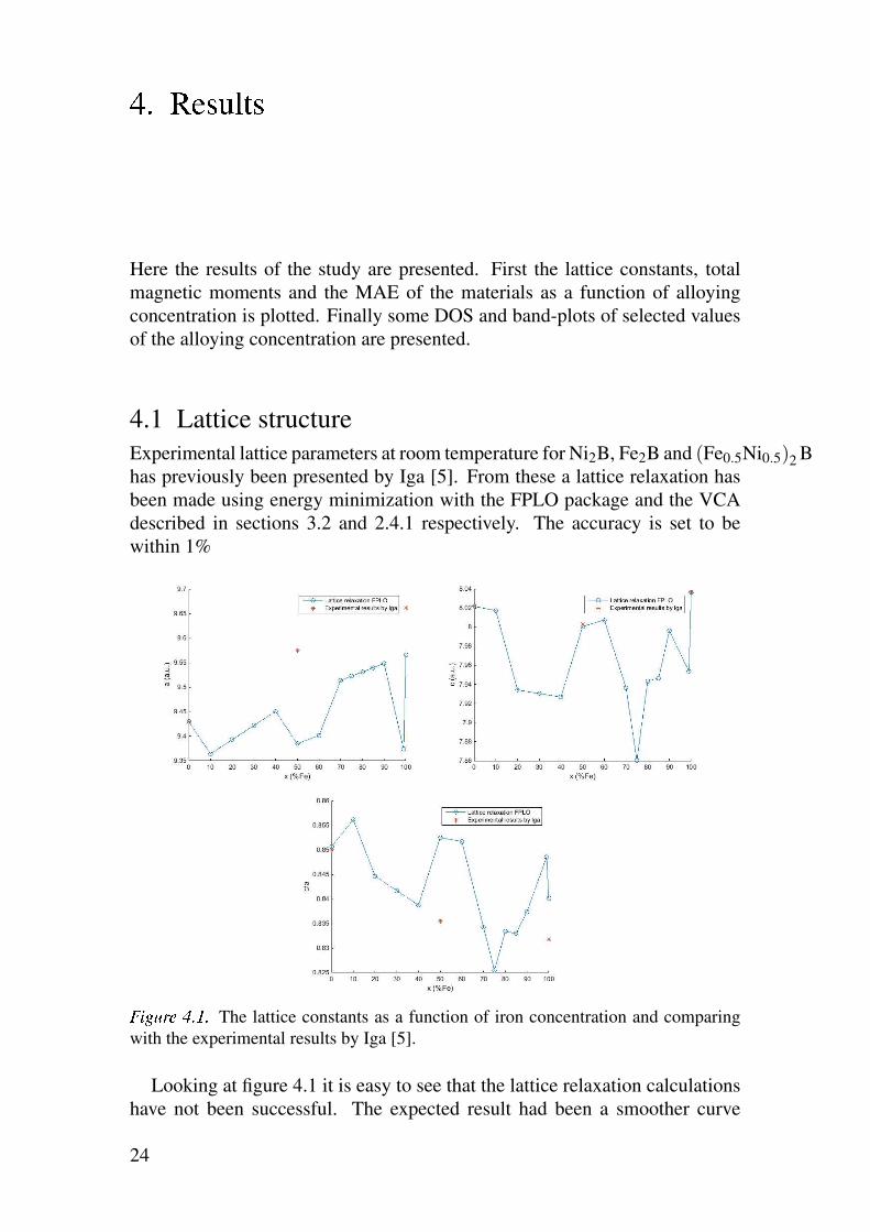
4.1 Lattice structure

Experimental lattice parameters at room temperature for Ni2B, Fe2B and (Fe0.5Ni0.5)2Bhas previously been presented by Iga [5]. From these a lattice relaxation has

been made using energy minimization with the FPLO package and the VCA

described in sections 3.2 and 2.4.1 respectively. The accuracy is set to be

within 1%

éêëìíî ïðñð The lattice constants as a function of iron concentration and comparing

with the experimental results by Iga [5].

Looking at figure 4.1 it is easy to see that the lattice relaxation calculations

have not been successful. The expected result had been a smoother curve

24

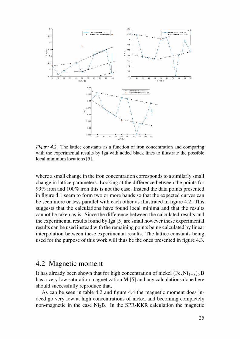
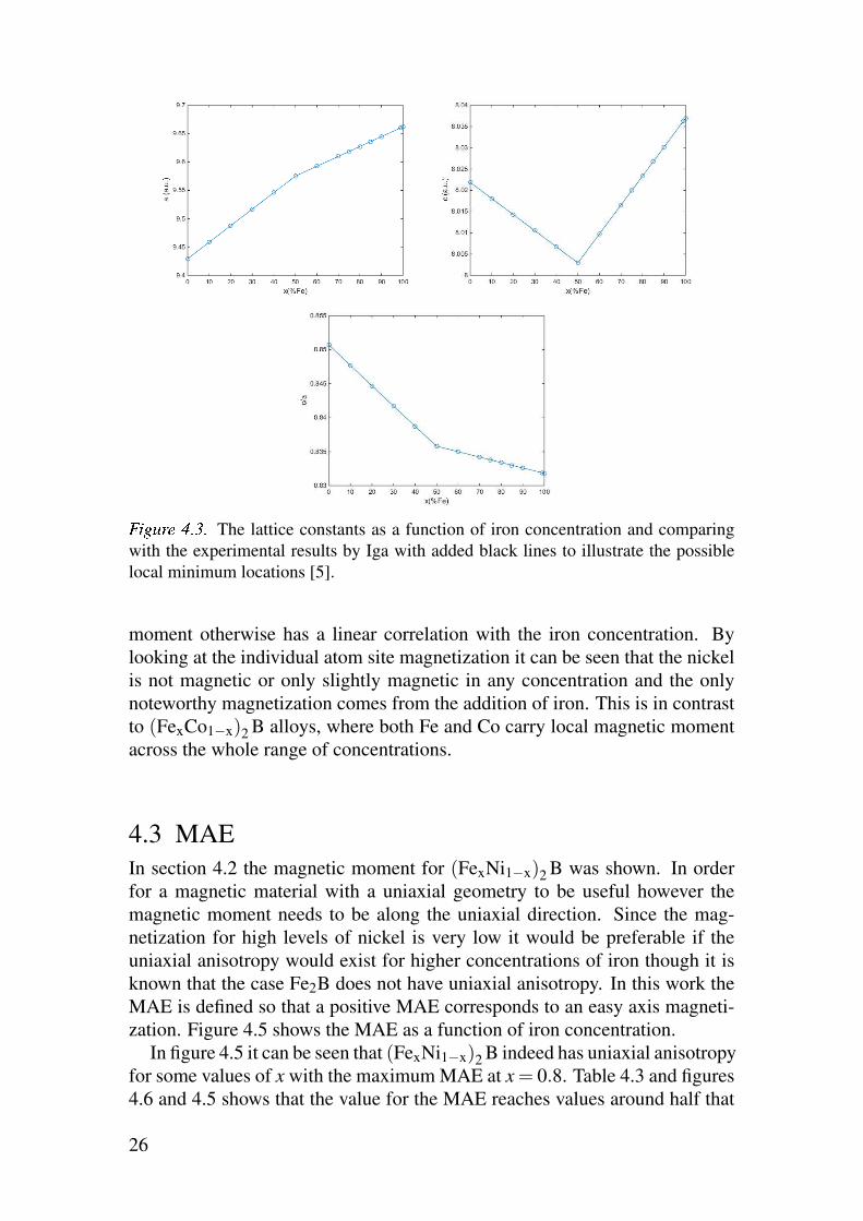
òóôõö÷ øùúù The lattice constants as a function of iron concentration and comparing

with the experimental results by Iga with added black lines to illustrate the possible

local minimum locations [5].

where a small change in the iron concentration corresponds to a similarly small

change in lattice parameters. Looking at the difference between the points for

99% iron and 100% iron this is not the case. Instead the data points presented

in figure 4.1 seem to form two or more bands so that the expected curves can

be seen more or less parallel with each other as illustrated in figure 4.2. This

suggests that the calculations have found local minima and that the results

cannot be taken as is. Since the difference between the calculated results and

the experimental results found by Iga [5] are small however these experimental

results can be used instead with the remaining points being calculated by linear

interpolation between these experimental results. The lattice constants being

used for the purpose of this work will thus be the ones presented in figure 4.3.

4.2 Magnetic moment

It has already been shown that for high concentration of nickel (FexNi1−x)2Bhas a very low saturation magnetization M [5] and any calculations done here

should successfully reproduce that.

As can be seen in table 4.2 and figure 4.4 the magnetic moment does in-

deed go very low at high concentrations of nickel and becoming completely

non-magnetic in the case Ni2B. In the SPR-KKR calculation the magnetic

25

ûüýþÿF The lattice constants as a function of iron concentration and comparing

with the experimental results by Iga with added black lines to illustrate the possible

local minimum locations [5].

moment otherwise has a linear correlation with the iron concentration. By

looking at the individual atom site magnetization it can be seen that the nickel

is not magnetic or only slightly magnetic in any concentration and the only

noteworthy magnetization comes from the addition of iron. This is in contrast

to (FexCo1−x)2B alloys, where both Fe and Co carry local magnetic moment

across the whole range of concentrations.

4.3 MAE

In section 4.2 the magnetic moment for (FexNi1−x)2B was shown. In order

for a magnetic material with a uniaxial geometry to be useful however the

magnetic moment needs to be along the uniaxial direction. Since the mag-

netization for high levels of nickel is very low it would be preferable if the

uniaxial anisotropy would exist for higher concentrations of iron though it is

known that the case Fe2B does not have uniaxial anisotropy. In this work the

MAE is defined so that a positive MAE corresponds to an easy axis magneti-

zation. Figure 4.5 shows the MAE as a function of iron concentration.

In figure 4.5 it can be seen that (FexNi1−x)2B indeed has uniaxial anisotropy

for some values of x with the maximumMAE at x= 0.8. Table 4.3 and figures

4.6 and 4.5 shows that the value for the MAE reaches values around half that

26

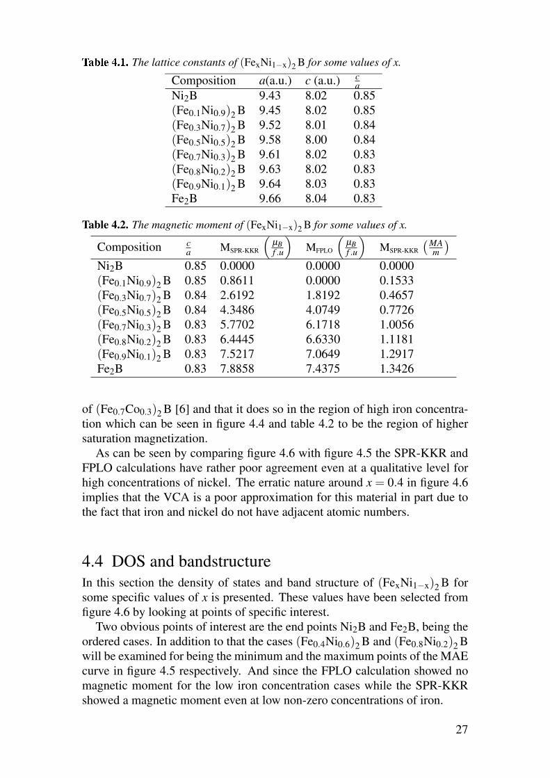
T The lattice constants of (FexNi1−x)2B for some values of x.

Composition a(a.u.) c (a.u.) ca

Ni2B 9.43 8.02 0.85

(Fe0.1Ni0.9)2B 9.45 8.02 0.85

(Fe0.3Ni0.7)2B 9.52 8.01 0.84

(Fe0.5Ni0.5)2B 9.58 8.00 0.84

(Fe0.7Ni0.3)2B 9.61 8.02 0.83

(Fe0.8Ni0.2)2B 9.63 8.02 0.83

(Fe0.9Ni0.1)2B 9.64 8.03 0.83

Fe2B 9.66 8.04 0.83

Table 4.2. The magnetic moment of (FexNi1−x)2B for some values of x.

Composition ca

MSPR-KKR

(

µB

f .u

)

MFPLO

(

µB

f .u

)

MSPR-KKR

(

MAm

)

Ni2B 0.85 0.0000 0.0000 0.0000

(Fe0.1Ni0.9)2B 0.85 0.8611 0.0000 0.1533

(Fe0.3Ni0.7)2B 0.84 2.6192 1.8192 0.4657

(Fe0.5Ni0.5)2B 0.84 4.3486 4.0749 0.7726

(Fe0.7Ni0.3)2B 0.83 5.7702 6.1718 1.0056

(Fe0.8Ni0.2)2B 0.83 6.4445 6.6330 1.1181

(Fe0.9Ni0.1)2B 0.83 7.5217 7.0649 1.2917

Fe2B 0.83 7.8858 7.4375 1.3426

of (Fe0.7Co0.3)2B [6] and that it does so in the region of high iron concentra-

tion which can be seen in figure 4.4 and table 4.2 to be the region of higher

saturation magnetization.

As can be seen by comparing figure 4.6 with figure 4.5 the SPR-KKR and

FPLO calculations have rather poor agreement even at a qualitative level for

high concentrations of nickel. The erratic nature around x = 0.4 in figure 4.6

implies that the VCA is a poor approximation for this material in part due to

the fact that iron and nickel do not have adjacent atomic numbers.

4.4 DOS and bandstructure

In this section the density of states and band structure of (FexNi1−x)2B for

some specific values of x is presented. These values have been selected from

figure 4.6 by looking at points of specific interest.

Two obvious points of interest are the end points Ni2B and Fe2B, being the

ordered cases. In addition to that the cases (Fe0.4Ni0.6)2B and (Fe0.8Ni0.2)2Bwill be examined for being the minimum and the maximum points of the MAE

curve in figure 4.5 respectively. And since the FPLO calculation showed no

magnetic moment for the low iron concentration cases while the SPR-KKR

showed a magnetic moment even at low non-zero concentrations of iron.

27

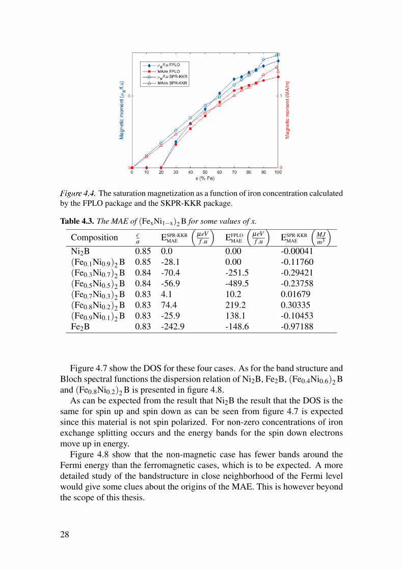
The saturation magnetization as a function of iron concentration calculated

by the FPLO package and the SKPR-KKR package.

Table 4.3. The MAE of (FexNi1−x)2B for some values of x.

Composition ca

ESPR-KKRMAE

(

µeVf .u

)

EFPLOMAE

(

µeVf .u

)

ESPR-KKRMAE

(

MJm3

)

Ni2B 0.85 0.0 0.00 -0.00041

(Fe0.1Ni0.9)2B 0.85 -28.1 0.00 -0.11760

(Fe0.3Ni0.7)2B 0.84 -70.4 -251.5 -0.29421

(Fe0.5Ni0.5)2B 0.84 -56.9 -489.5 -0.23758

(Fe0.7Ni0.3)2B 0.83 4.1 10.2 0.01679

(Fe0.8Ni0.2)2B 0.83 74.4 219.2 0.30335

(Fe0.9Ni0.1)2B 0.83 -25.9 138.1 -0.10453

Fe2B 0.83 -242.9 -148.6 -0.97188

Figure 4.7 show the DOS for these four cases. As for the band structure and

Bloch spectral functions the dispersion relation of Ni2B, Fe2B, (Fe0.4Ni0.6)2Band (Fe0.8Ni0.2)2B is presented in figure 4.8.

As can be expected from the result that Ni2B the result that the DOS is the

same for spin up and spin down as can be seen from figure 4.7 is expected

since this material is not spin polarized. For non-zero concentrations of iron

exchange splitting occurs and the energy bands for the spin down electrons

move up in energy.

Figure 4.8 show that the non-magnetic case has fewer bands around the

Fermi energy than the ferromagnetic cases, which is to be expected. A more

detailed study of the bandstructure in close neighborhood of the Fermi level

would give some clues about the origins of the MAE. This is however beyond

the scope of this thesis.

28

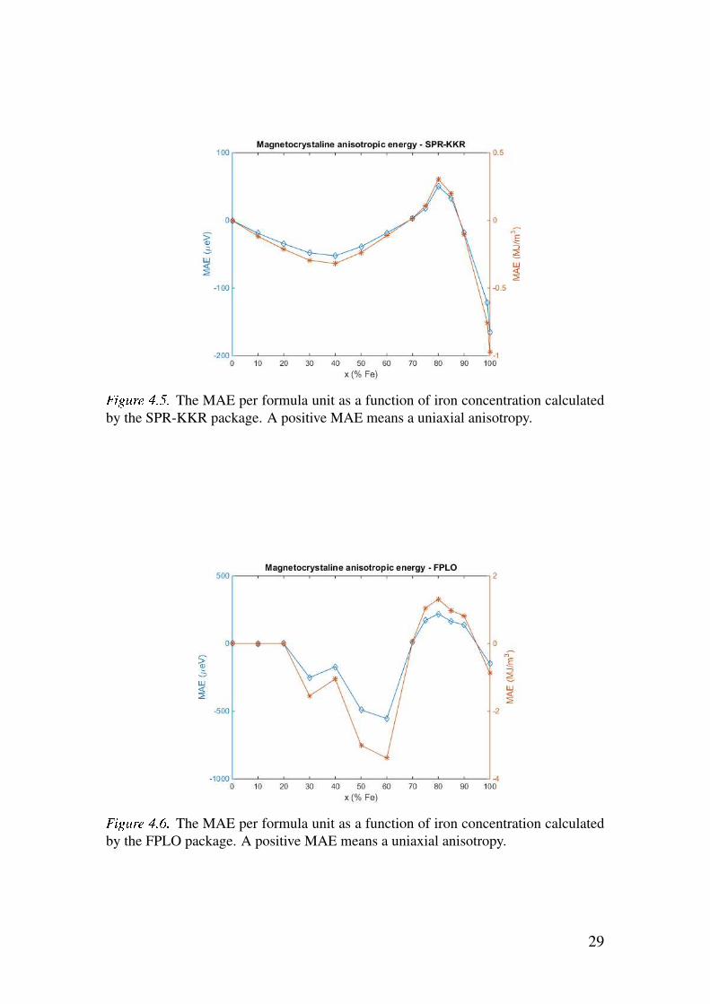
The MAE per formula unit as a function of iron concentration calculated

by the SPR-KKR package. A positive MAE means a uniaxial anisotropy.

The MAE per formula unit as a function of iron concentration calculated

by the FPLO package. A positive MAE means a uniaxial anisotropy.

29

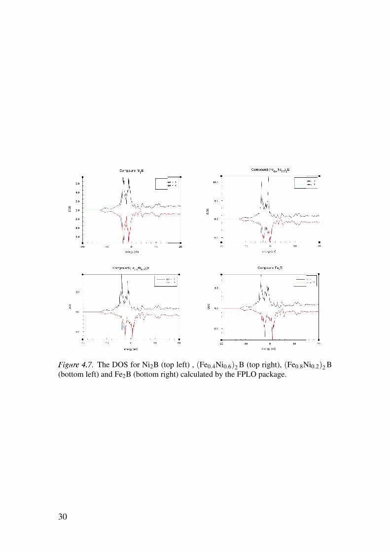
! "#$# The DOS for Ni2B (top left) , (Fe0.4Ni0.6)2B (top right), (Fe0.8Ni0.2)2B(bottom left) and Fe2B (bottom right) calculated by the FPLO package.

30

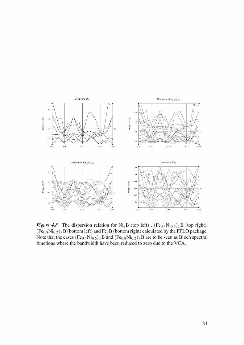
%&'()* +,-, The dispersion relation for Ni2B (top left) , (Fe0.4Ni0.6)2B (top right),

(Fe0.8Ni0.2)2B (bottom left) and Fe2B (bottom right) calculated by the FPLO package.

Note that the cases (Fe0.4Ni0.6)2B and (Fe0.8Ni0.2)2B are to be seen as Bloch spectral

functions where the bandwidth have been reduced to zero due to the VCA.

31

5. /012346701

This work aims to give a theoretical background of permanent magnets and

the computational methods used to study them. In addition to that theoretical

calculation of the magnetization and MAE of (FexNi1−x)2B has been pre-

sented. Apart from saturation magnetization and MAE the Curie temperature

is an important property for a permanent magnet. Studying the Curie temper-

ature is beyond the scope of this study however. A uniaxial anisotropy was

found around x= 0.8 and though the MAE is lower than other 3d-based mag-

netic materials it is comparatively cheap while still being higher than ferrite

magnets and may still be worthy of further investigation since the magnetic

moment was shown to be satisfactory at this concentration of iron and nickel.

Permanent magnets that are not made from rare-earth metals or other heavy

elements is still an emerging field and the task is far from trivial. Trade-offs

might need to be made concerning effectiveness or stability versus cost. Sev-

eral candidates have been found however and many of them do seem like vi-

able choices. Specifically it has been shown that a permanent magnet good

enough for industrial application without containing materials heavier than

the 3d transition metals is a viable pursuit.

32

R898:8;<8=

[1] M. J. Kramer, R. W. McCallum, I. A. Anderson, and S. Constantinides.

Prospects for non-rare earth magnets for traction motors and generators.

Journal of The Minerals, Metals & Materials Society, 64(7):752–763, 2012.

[2] David Kramer. Concern grows over china’s dominance of rare-earth metals.

Physics Today, 63(5):22, 2010.

[3] J. M. D. Coey. Hard magnetic materials: A perspective. Advances in Magnetics,

47(12):4671–4681, 2011.

[4] P-K Tse. China’s rare-earth industry. U.S. Geological Survey, 2011.

[5] Atushi Iga. Magnetocrystalline anisotropy in (Fe1−xNix)2B system. Japanese

Journal of applied physics, 9:414–415, 1970.

[6] Alexander Edström. Theoretical Magnet Design - From the electronic structure

of solid matter to new permanent magnets. Licentiate thesis, Uppsala

Universitet, 2014.

[7] A. Edström, M. Werwinski, D. Iusan, J. Rusz, O. Eriksson, K. P. Skokov, I. A.

Radulov, S. Ener, M. D. Kuz’min, J. Hong, M. Fries, D. Yu. Karpenov,

O. Gutfleisch, P. Toson, and J. Fidler. Magnetic properties of (Fe1−xCox)2balloys and the effect of doping by 5d elements. Physical review B,

92(17):174413, 2015.

[8] K. D. Belashchenko, L. Ke, M. Däne, L. X. Benedict, T. N. Lamichhane,

V. Taufour, A. Jesche, S. L. Bud’ko, P. C. Canfield, and V. P. Antropov. Origin

of the spin reorientation transitions in (Fe1−xCox)2b alloys. Applied PhysicsLetters, 106(6):062408, 2015.

[9] W. Pauli. Zur Quantenmechanik des magnetischen Elektrons. Zeitschrift für

Physik, 43(9-10):601–623, 1927.

[10] C. G. Darwin. Free motion in the wave mechanics. Proceedings of the Royal

Society A., 117(776):258–293, 1927.

[11] P. A. M. Dirac. The quantum theory of the electron. Proceedings of the Royal

Society A, 117(778):610–624, 1928.

[12] P. A. M. Dirac. The quantum theory of the electron. part ii. Proceedings of the

Royal Society A., 118(779):351–361, 1928.

[13] R. Feder, F. Rosicky, and B. Ackermann. Relativistic multiple scattering theory

of electrons by ferromagnets. Zeitschrift für Physik B, 52:31–36, 1983.

[14] P. Strange, J. Staunton, and B. L. Gyorffy. Relativistic spin-polarised scattering

theory - solution of the single-site problem. Journal of Physics C: Solid State

Physics, 17(19):3355–3371, 1984.

[15] G. Schadler, P. Weinberger, A. M. Boring, and R. C. Albers. Relativistic

spin-polarized electronic structure of Ce and Pu. Physical Review B,

34(2):713–722, 1986.

[16] E. van Lenthe, J. G. Snijders, and E. J. Baerends. The zero-order regular

approximation for relativistic effect: .The effect of spin-orbit coupling in closed

shell molecules. The Journal of Chemical Physics, 105(15):6505–6516, 1996.

33

[>?@ R. L. Martin. All-electron relativistic calculations on AgH. an investigation of

the Cowan-Griffin operator in a molecular species. Journal of Physical

Chemistry, 87(5):750–754, 1982.

[18] H. Ebert, P Strange, and B. L. Gyorffy. The influence of relativistic effects on

the magnetic moments and hyperfine fields of Fe, Co and Ni. Journal of Physics

F: Metal Physics, 18(7):135–139, 1988.

[19] E. C. Stoner and E. P. Wohlfarth. A mechanism of magnetic hysteresis in

heterogenous alloys. Philosophcal transactions of the Royal Society of London

A, 240(826), 1948.

[20] S Chikazumi. Physics of Ferromagnetism. Oxford University Press, 1997.

[21] H. Ebert, D. Ködderitzsch, and J. Minár. Calculating condensed matterproperties using the KKR-Green’s function method - recent developments andapplications. Reports on Progress in Physics, 74(9):095401, 2011.

[22] L. Szunyogh, B. Újfalussy, and P Weinberger. Magnetic anisotropy of ironmultilayers on .Au(001): First-principles calculations in terms of the fullyrelativistic spin-polarized screened KKR method. Physical Review B,51(15):9552–9559, 1995.

[23] W Koch and M. C. Holthausen. A Chemist’s Guide to Density Funcitonal

Theory. Wiley-VCH, 2001.[24] J. C. Slater. A simplification of the hartree-fock method. Physical Review,

81(3):385–390, 1951.[25] W. Kohn and L. J. Sham. Self-consistent equations including exchange and

correlation effects. Physical Review A, 140(4):1133–1138, 1965.[26] P. Hohenberg and W. Kohn. Inhomogeneous electron gas. Physical Review B,

136(3):864–871, 1964.[27] T. L. Gilbert. Hohenberg-kohn theorem for nonlocal external potentials.

Physical Review B, 12(6):2111–2120, 1975.[28] J. Garza, R. Vargas, J. A. Nichols, and D. A. Dixon. Orbital energy analysis

with respect to lda and self-interaction corrected exchange only potentials. TheJournal of Chemical Physics, 114(2):639–651, 2001.

[29] P. M. Laufer and J. B. Krieger. Test of density-functional approximations in anexactly soluble model. Phsyical Review A, 33(3):1480–1491, 1986.

[30] J. P. Perdew and M. Levy. Physical content of the exact Kohn-Sham orbitalenergies: Band gaps and derivative discontinuities. Physical Review Letters,51(20):1884–1887, 1983.

[31] A. I. Anisimov, F. Aryasetiawan, and A. I. Lichtenstein. First-principlescalculations of the electronic structure and spectra of strongly correlatedsystems: the lda + u method. Journal of Physics: Condensed Matter,9:767–808, 1997.

[32] A. Kabir, V. Turkowski, and T. S. Rahman. A DFT + nonhomogeneous DMFTapproach for finite systems. Journal of Physics: Condensed Matter, 27(12):1–5,2015.

[33] I. A. Nekrasov, V. S. Pavlov, and Sadovkii M. V. Consistent LDA’ + DMFT - anunambiguous way to avoid double counting problem: NiO test. JETP Letters,95(11):581–585, 2012.

[34] C. Stampfl, W. Mannstadt, R. Asahi, and A. J. Freeman. Electronic structureand physical properties of early transition metal mononitrides:

34

DABCEGHIJKBLtional theory lda, gga, and screened-exchange lda flapw

calculations. Physical Review B, 63(15):1–11, 2001.

[35] Y. S. Mohammed, Y. Yan, H. Wang, K. Li, and X. Du. Stability of

Ferromagnetism in Fe, Co, and Ni metals under high pressure with GGA and

GGA+U. Journal of Magnetism and Magnetic Materials, 322(6):653–657,

2010.

[36] J. P. Perdew, K. Burke, and M. Ernzerhof. Generalized gradient approximation

made simple. Physical Review Letters, 77(18):3865–3868, 1996.

[37] L. Bellache and D. Vanderbilt. Virtual crystal approximation revisited:

Application to dielectric and piezoelectric properties of perovskites. Physical

Review B, 61(12):7877–7882, 1999.

[38] P. Söderlind, O. Eriksson, and B. Johansson. Spin and orbital magnetism in

Fe-Co and Co-Ni alloys. Physical Review B, 45(22):12911–12916, 1992.

[39] J. M. Schoen. Augmented-plane-wave virtual crystal approximation. Physical

Review, 184(3):858–863, 1969.

[40] I. Turek, J. Kudrnovský, and K. Carva. Magnetic anisotropy energy of

disordered tetragonal Fe-Co systems from ab initio alloy theory. Physical

Review B, 86(17):174430, 2012.

[41] K. Koepernik and H. Eschrig. Full-potential nonorthogonal local-orbital

minimum-basis band-structure scheme. Physical Review B, 59(3):1743–1757,

1999.

[42] P. Soven. Coherent-potential model of substitutional disordered alloys. Physical

Review, 156(3):809–813, 1966.

[43] D. D. Johnson, D. M. Nicholson, F. J. Pinski, B. L. Györffy, and G. M. Stocks.

Total-energy and pressure calculations for random substitutional alloys.

Physical Review B, 41(14):9701–9716, 1990.

[44] J. L. Beeby. The density of electros in a perfect or imperfect lattice.

Proceedings of the Royal Society A, 302:113–136, 1967.

[45] J. S. Faulkner and G. M. Stocks. Calculating properties with the

coherent-potential approximation. Physical Review B, 21(8):3222–3244, 1980.

[46] A. M. Tsvelik. Quantum Field Theory in Condensed Matter Physics.

Cambridge University Press, 2003.

[47] A. Ernst. Multiple-scattering theory: new developments and applications. Phd

thesis, Martin-Luther-Universität Halle-Wittenberg, 2007.

[48] F. Yonezawa and K. Morigaki. Coherent potential approximation-basic concepts

and applications. Supplement of the Progress of Theoretical Physics, 53, 1973.

[49] H Ebert. A spin polarized relativistic Korringa-Kohn-Rostoker (SPR-KKR)

code for Calculating Solid State Properties. 2012.

[50] D. A. Biava, S. Ghosh, D. D. Johnson, W. A. Shelton, and A. V. Smirnov.

Systematic, multisite short-range-order corrections to the electronic structure of

disordered alloys from first principles: The KKR nonlocal CPA from the

dynamical cluster approximation. Physical Review B, 72(11):113105, 2005.

[51] G. M. Stocks, W. M. Temmerman, and B. L. Gyorffy. Complete solution of the

Korringa-Kohn-Rostoker Coherent-Potential-Aproximaiton equations: Cu-Ni

alloys. Physical Review Letters, 41(5):339–343, 1978.

[52] J. Korringa. On the calculation of the energy of a Bloch wave in a metal.

Physica, 13(6-7):392–400, 1947.

35

MNOP W. Kohn and N. Rostoker. Solution of the Schrödinger equation in periodic

lattices with an application to metallic lithium. Physical Review,

94(5):1111–1120, 1954.

[54] R. Zeller, P. H. Dederichs, B. Újfalussy, L. Szunyogh, and P. Weinberger.Theory and convergence properties of the screened .Korringa-Kohn-Rostokermethod. Physical Review B, 52(12):8807–8812, 1995.

[55] I. Opahle, K. Koepernik, and H. Eschrig. Full-potential band-structurecalculation of iron pyrite. Physical Review B, 60(20):14035–14041, 1999.

[56] N. W. Ashcroft and N. D. Mermin. Solid State Physics. Brooks/Cole, Belmont,USA, 1976.

[57] N. Papanikolaou, R. Zeller, and P. H. Dederichs. Conceptual improvements ofthe kkr method. Journal of Physics: Condensed Matter, 14(11):2799–2823,2002.

[58] R. Zeller. An elementary derivation of Lloyd’s formula valid for full-potentialmultiple-scattering theory. Journal of Physics: Condensed Matter,16(36):6453–6468, 2004.

[59] B. Drittler, M. Weinert, R. Zeller, and P. H. Dederichs. First-principlescalculation of impurity-solutions energies in Cu and Ni. Physical Review B,39(2):930–939, 1989.

36