Patterns of synchronization in the hydrodynamic coupling of active colloids

Giovanni M. Cicuta,1, 2 Enrico Onofri,1, 2 Marco Cosentino Lagomarsino,3, 4 and Pietro Cicuta5

1Dipartimento di Fisica, Universita di Parma, Parco Area delle Scienze 7A, 43100 Parma, Italy2INFN, Sez.di Milano-Bicocca, Gruppo Collegato di Parma

3Genomic Physics Group, FRE 3214 CNRS “Microorganism Genomics”4University Pierre et Marie Curie, 15, rue de l’ Ecole de Medecine Paris, France

5Cavendish Laboratory and Nanoscience Centre, University of Cambridge, Cambridge CB3 0HE, U. K.∗

A system of active colloidal particles driven by harmonic potentials to oscillate about the verticesof a regular polygon, with hydrodynamic coupling between all particles, is described by a piece-wiselinear model which exhibits various patterns of synchronization. Analytical solutions are obtainedfor this class of dynamical systems. Depending only on the number of particles, the synchronizationoccurs into states in which nearest neighbors oscillate either in-phase, or anti-phase, or in phase-locked (time-shifted) trajectories.

I. INTRODUCTION

In passive colloidal particle systems, hydrodynamic in-teractions determine the dissipative and dynamical be-havior, rather than the real-space conformation; as suchthey influence the response properties rather than theequilibrium behavior. However in actively driven sys-tems that settle into a steady state, it can be the hydro-dynamic interactions that determine the characteristicsof the steady state. For example, in biological flows actu-ated by cilia [1], the hydrodynamic coupling is possiblythe most important feature involved in the synchroniza-tion of cilia beats [2].

In this paper we analyze theoretically a very simple dy-namical system which was recently proven to adequatelydescribe the motion of a system of colloidal spheres,maintained in oscillations by optical traps [3, 4]. Mo-tion occurs at low Reynolds number [5], and hydrody-namic forces between particles depend on the relativevelocity [6, 7].

The remarkable feature of the model is that the hy-drodynamic interaction of the spheres leads to the syn-chronization of their phases, for any number of beads,for all initial conditions and for generic values of physicalparameters (sphere size, viscosity of the fluid, stiffnessof the forces). The synchronized state depends on thenumber of spheres, and on wether the optical traps pro-vide attractive or repulsive forces. This produces a richpattern of synchronized configurations.

The system of equations of motion is piece-wise linear.It has periodic solutions, which are linear combinationsof the normal modes. Whilst we do not have a mathe-matical proof which would explain why this dynamicalsystem always converges to a synchronized solution, wehave performed a normal mode analysis and we showthat based on this it is possible to predict which synchro-nized solution is dominant. This analytical argumentis in agreement with extensive numerical integration ofthe deterministic (no thermal noise) system, and with

∗ correspondence to:giovanni.cicuta@fis.unipr.it

the experiments and simulations reported in the com-panion paper which include the effect of thermal noise [4].

Let us outline the physical system and its model,leading to the dynamic deterministic system of equationof motion which will be our main concern in the nextsection. We refer the reader to the literature whichdetails a series of experiments and their analysis. Byfocused laser beams, it was possible to confine effectivelyan array of micron-sized beads, each one into a harmonicwell. These colloidal particles interact exclusivelythrough the hydrodynamic coupling. The collective fluc-tuation modes resulting from hydrodynamic interactionshave been studied in linear arrays [8] and ring arrays[9, 10]. The “geometric switch” active driving model westudy here was proposed in the context of cilia by [1]; itwas studied analytically for two beads and for infinitelinear chains by Cosentino Lagomarsino and Bassettiin [11], where they showed that an infinite linear chainof oscillators can sustain a traveling wave solution. Thismodel was then realized experimentally in [3], by usingoptical tweezers to maintain a pair of colloidal spheresin oscillation by switching the positions of optical trapswhen a sphere reaches its limit position. This rule leadsto oscillations that are bounded in amplitude but free inphase and period. The interaction between the oscilla-tors is only through the hydrodynamic flow induced bytheir motion; the colloidal particles in the experimentare subject to Brownian thermal fluctuations as wouldalso be found in a biological context. This system oftwo spheres in harmonic traps leads to synchronizedmotion in anti-phase [3]. A companion paper to this onereports experimental results and the effect of noise, inthe system of actively moving traps for many particles[4]. Very recently, Wollin and Stark [12] re-consideredthis model for the case of a chain of driven oscillators,performing numerical simulations showing that forvarious potentials and forms of coupling the dynamicsystem evolves to a synchronized state which may beinterpreted as a (discretized) wave propagating throughthe chain. The form of the wave depends on the drivingforces and their being attractive or repulsive. This

arX

iv:1

110.

1524

v2 [

cond

-mat

.sta

t-m

ech]

10

Oct

201

1

2

chain is closely related to the array of driven oscillatorsstudied in this paper and experimentally observed [4].The main differences are the geometry (our oscillatorsare tangential to a ring) and the symmetry (in ourmodel, the driving force acts in the same way in thetwo phases of each cycle, i.e. as each oscillator movesforward or backward).The periodic solutions analytically obtained in thispaper may be interpreted as a wave propagating alongthe border of the ring, clockwise or anti-clockwise.Indeed if xj(t) describes the motion of the jth-oscillator,our periodic solutions have the form xj+1(t+∆) = xj(t),where ∆ is a fixed, positive or negative, time interval,independent on j. In a recent paper [13] Uchida andGolestanian derived generic conditions on the drivenoscillators to synchronize due to the hydrodynamicinteractions. However, as it was already noted in [12],it is not clear if such conditions would apply to the“geometric switch” model.

The paper is organized as follows: Section II outlinesthe model and the associated dynamical system. Sec-tion III shows the normal mode analysis that allows(in principle) a completely analytical determination ofthe periodic solutions of the system for any number ofparticles. Section IV describes the periodic solutions,if the number of particles is 3, 4, 5 and the dominantsolution for any number of particles. In Section V wereplace the attractive forces with repulsive ones andobtain periodic solutions trivially related to the previousones.

II. THE MODEL

Let us first describe the system in absence of hydro-dynamic coupling between particles. Fig. 1(a) shows aring of radius R, with n spheres depicted at the ver-tices of a regular n−polygon. Each vertex is the cen-ter of small oscillations of a particle bound to the ring.The jth-particle performs oscillations about the position

Rj = Rθ(0)j = R 2π

n (j − 1), with j = 1, 2, · · · , n. Oneach side of this position, the amplitude of the oscilla-tion is λ/2 − ξ. This is assumed to be so small thatwe may replace the path on the arc with a segment ofstraight line, tangent to the ring, and then consider themotion of the jth-particle on the tangent with a variablexj : −(λ/2 − ξ) ≤ xj(t) ≤ λ/2 − ξ. The oscillations aredriven by an attractive harmonic potential (or repulsiveharmonic potential, as discussed later in section V) withcenter at s = ±λ/2. In the hydrodynamic regime whereReynolds number is much smaller then unity, the inertialterm may be neglected.

An oscillation is set up that has fixed amplitude, butfree phase and period. This is realized through a “ge-ometric switch” condition. First the trap is set at λ/2,and particle moves along the positive x axis according to

x(t)

x(t)

t

x(t)(b)

FIG. 1. (Color online) (a) Diagram of the ring arrangementwith n = 6 driven oscillators, illustrating the notation used inthe main text. Colloidal particles move tangential to the ring,with the center of oscillations being the vertices of a regularn−polygon. The local tangential co-ordinate system is shownfor one of the top particles. The particle configuration (soliddisks) corresponds to an in-phase condition, when all 6 par-ticles have just reached the geometric switch boundary. Theparticles are driven by harmonic traps towards the minimumof the potential, but they will reach first the other geomet-ric switch boundary, when at the position indicated with opendisks. This work also considers harmonic potentials with neg-ative stiffness (i.e. repulsive) in section V. (b) Trajectory ofa driven oscillator with attractive driving force, uncoupled toother oscillators; x(t) is measured along the tangential direc-tion.

the differential equation

γ0x(t) + κ

(x(t)− λ

2

)− f(x) = 0,

where κ is the stiffness of the harmonic force, τ0 = γ0/κis the relaxation time, and f is a stochastic force due tothermal agitation of the fluid, which will be neglected inthis work. As the particle reaches the position λ

2 − ξ, theattractive harmonic potential is moved at the position−λ2 . The particle inverts its overdamped motion until it

reaches the position −λ2 + ξ. At this time, the poten-tial jumps again. The resulting oscillatory motion (thisis either a single bead, or a bead in a system with nocoupling), neglecting any stochastic force, is depicted inFig. 1(b). The period T0 of these uncoupled oscillations

3

is

T0

2τ0= log

λ− ξξ

.

In a system of n beads, at any given time, the set ofpositions of the particles is a n−th dimensional vector~x(t) = {x1(t), x2(t), · · · , xn(t)}. In the absence of thehydrodynamic coupling, each particle would perform thesame periodic motion described above, a set of periodicoverdamped relaxations. For any pair of particles,the “phase differences” xj(t) − xk(t) would be set byinitial conditions (typically some random values) and beconstant in time.

Let us now include the hydrodynamic interaction.The motion of the jth-particle originates a force on the

ith-particle ~f i,jα = (H−1)α,βi,j v(j)β , where H is the Oseen

tensor [5]. In agreement with previous analysis [8–10] weare led to the system of equations

~Fi −∑nj=1H

−1i,j

d~rj(t)dt + ~fi(t) = 0, i = 1, 2 · · · , n

~ri(t) · ~t(~ri) = 0, ~t(θ) =

(− sin θcos θ

).

(1)

The deterministic force ~Fi acting on the i-th particleis a harmonic force, tangent to the ring, with the “geo-metric switch” rule,

~Fi = −κ[xi(t)∓

λ

2

]~t

(2π(i− 1)

n

),

where±λ2 is the coordinate of the bottom of the harmonicwell.

The stochastic force fi(t) in Eq. 1 represents the ther-mal noise on the i-th particle, and it can be assumed that< fi(t) >= 0, < fi(t1)fj(t2) >= 2(β)−1 (H−1)ij δ(t1 −t2), β−1 = kBT [8]. ~t(~ri) is a versor tangent to the ring,at the position ~ri , with anti-clockwise direction. Forsmall oscillations, the Oseen tensor can be approximatedby inserting the fixed distances among centers of oscilla-tions, then:

γ0Hαβij = δijδαβ + (1− δij)

3a

4rij

(δαβ +

rαijrβij

r2ij

),

where

(rjxrjy

)'(RjxRjy

)= R

(cos(j − 1)2π/nsin(j − 1)2π/n

)with rαij ' Rαj −Rαi = −rαji, and α = 1, 2.

We project the equations of the linearized Langevin-Oseen system along the tangents, replace the globalcoordinates of the jth-particle ~r(j) with the local one-dimensional coordinate x(j) and neglect the stochasticforce, to obtain the deterministic linear system whichholds in the time interval where no particle hits its leftor right boundary ±(λ2 − ξ):(

I +3a

8RCn

)(~x(t)− ~s) + τ0

d

dt~x(t) = 0, (2)

Initial conditions

x(t0)

s(0)x(t) ; t0<t<t1

s(0)

Normal mode solutionpropagated until first switch

x(t1)

s(1)

Updated initial conditionand switch state

Study the iterative discrete map {ti, x(ti), s(i)} i=1,2...

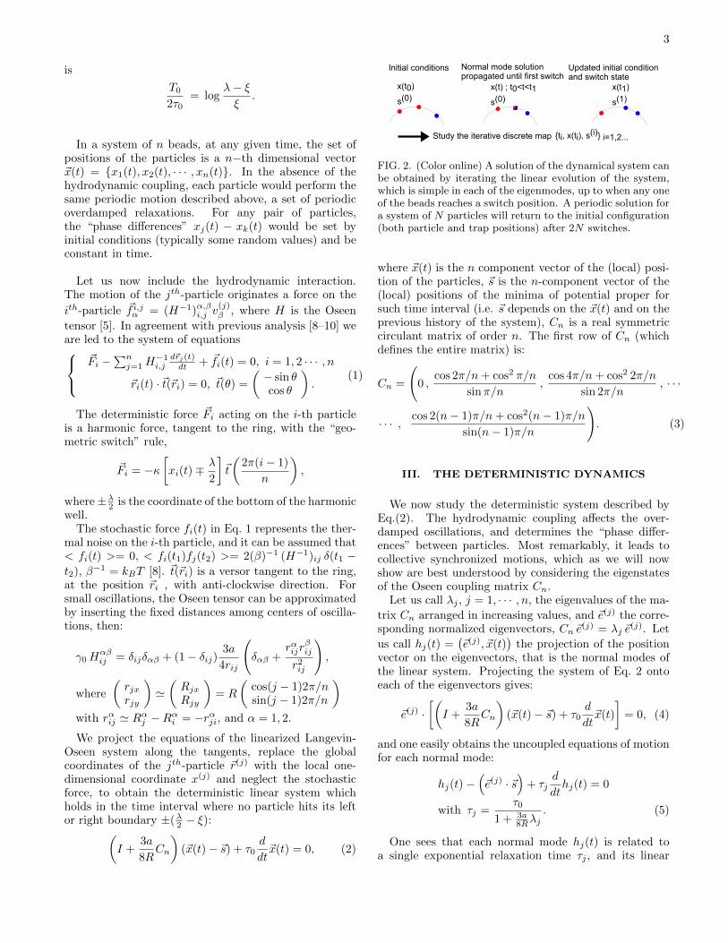
FIG. 2. (Color online) A solution of the dynamical system canbe obtained by iterating the linear evolution of the system,which is simple in each of the eigenmodes, up to when any oneof the beads reaches a switch position. A periodic solution fora system of N particles will return to the initial configuration(both particle and trap positions) after 2N switches.

where ~x(t) is the n component vector of the (local) posi-tion of the particles, ~s is the n-component vector of the(local) positions of the minima of potential proper forsuch time interval (i.e. ~s depends on the ~x(t) and on theprevious history of the system), Cn is a real symmetriccirculant matrix of order n. The first row of Cn (whichdefines the entire matrix) is:

Cn =

(0 ,

cos 2π/n+ cos2 π/n

sinπ/n,

cos 4π/n+ cos2 2π/n

sin 2π/n, · · ·

· · · , cos 2(n− 1)π/n+ cos2(n− 1)π/n

sin(n− 1)π/n

). (3)

III. THE DETERMINISTIC DYNAMICS

We now study the deterministic system described byEq.(2). The hydrodynamic coupling affects the over-damped oscillations, and determines the “phase differ-ences” between particles. Most remarkably, it leads tocollective synchronized motions, which as we will nowshow are best understood by considering the eigenstatesof the Oseen coupling matrix Cn.

Let us call λj , j = 1, · · · , n, the eigenvalues of the ma-

trix Cn arranged in increasing values, and ~e(j) the corre-sponding normalized eigenvectors, Cn ~e

(j) = λj ~e(j). Let

us call hj(t) =(~e(j), ~x(t)

)the projection of the position

vector on the eigenvectors, that is the normal modes ofthe linear system. Projecting the system of Eq. 2 ontoeach of the eigenvectors gives:

~e(j) ·[(I +

3a

8RCn

)(~x(t)− ~s) + τ0

d

dt~x(t)

]= 0, (4)

and one easily obtains the uncoupled equations of motionfor each normal mode:

hj(t)−(~e(j) · ~s

)+ τj

d

dthj(t) = 0

with τj =τ0

1 + 3a8Rλj

. (5)

One sees that each normal mode hj(t) is related toa single exponential relaxation time τj , and its linear

4

differential equation is homogeneous, if and only if theterm

(~e(j) · ~s

)vanishes. In general, this is not the case.

A solution of the dynamical system can be obtainedwith the following simple strategy (Fig 2): Given initialpositions ~x(t0) and initial configuration of potential ~s(0),the evolution is trivially evaluated up to the time t1of the first hit. At this time one entry of the vector~s changes sign, and the uncoupled system of Eq. 5 isagain evaluated with the new constant vector ~s(1) up tothe hit at time t2. A basic role is then played by thecontinuity of each mode at the time of the hits: the fi-nal value before the hit becomes the new initial condition.

The rotational discrete symmetry of the problem al-lows a detailed analytic study of the coupling matrix Cn.The most relevant features are the following:(1) for every n being even integer, the lowest eigen-value λ1 is a singlet, and its corresponding eigenvectoris ~e(1) = 1√

n(1,−1, 1, · · · ,−1);

(2) for every n being odd integer n ≥ 5, the lowest eigen-value λ1 is a doublet. The two eigenvectors may be writ-ten as

~e(1) =1√n

(1, cos(n− 1)π/n, cos 2(n− 1)π/n, · · ·

· · · cos(n− 1)2π/n),

~e(2) =1√n

(0, sin(n− 1)π/n, sin 2(n− 1)π/n, · · ·

· · · sin(n− 1)2π/n)

;

(3) for every n, the matrix Cn has the eigenvector~e = 1√

n(1, 1, 1, · · · , 1). Only for n = 3 this constant

eigenvector corresponds to the lowest eigenvalue λ1;(4) Since tr[Cn] = 0, the lowest eigenvalue λ1 < 0, andtherefore the relaxation time τ1 > τ0 for every n.

IV. THE ANALYTIC ASYMPTOTICSOLUTIONS

The dynamics of the system depends on three combi-nations of parameters: τ0 = γ0/κ sets the unit of timefor the evolution between hits; 3a/(8R) measures thestrength of the hydrodynamic interaction, and is limitedby the bound d = 2R sinπ/n � 2a. Finally ξ/λ, with0 < ξ/λ < 1/2, fixes the amplitude of the oscillations.The periodic solutions are here obtained for arbitrary val-ues of the parameters (within the physical bounds givenabove). The plots for three and four particles, in Fig-

ures 3, 5, 10, have ξ/λ = 1/4 and 3a/(8R) =√

3/5. Theplots for five particles, in Figures 7 and 8 have ξ/λ = 1/4and 3a/(8R) = 0.2. These values of 3a/(8R) are muchgreater than sensible experimental values [3, 4], but arechosen here to spread the relaxation times τj , so empha-sizing the differences between periodic solutions.

A. Case of n = 3

For n = 3 the lowest eigenvalue of the coupling matrixC3 is λ1 = − 1√

3, a singlet. The next eigenvalue is a

doublet λ2 = λ3 = 12√

3. The corresponding eigenvectors

may be written:

~e(1) =1√3

111

, ~e(2) =1√2

01−1

, ~e(3) =1√6

−211

.

(6)

We find the following periodic solutions for the system,here listed in order of decreasing duration of the periods:(a) the three particles are synchronized in-phase;(b) a pair of equivalent solutions, where the trajectoriesare phase-locked (more precisely, time-shifted).

Let us consider first case (a), with the configuration ofparticles in-phase, i.e. such that x1(t) = x2(t) = x3(t).The vector of the positions of the potential is

~s = ±λ2

111

.

The lowest normal mode is h1(t) =1√3

(x1(t) + x2(t) + x3(t)) →√

3x1(t) and it solves

the equation:

h1(t)−(~e(1) · ~s

)+ τ1

d

dth1(t) = 0 ,

where(~e(1) · ~s

)= ±√

3λ

2, and τ1 = τ0

(1−√

3a

8R

)−1

.

Since(~e(j) · ~s

)= 0 for j 6= 1, the modes h2(t), h3(t)

solve a homogeneous equation and the choice h2(t) =h3(t) = 0 is consistent. As the three particles hit si-multaneously a geometric switch border, all of ~s → −~s.Therefore by continuity one obtains the opposite motionin the following time interval. The three particles per-form in-phase oscillations, satisfying the same equationas if they were un-coupled, as depicted on Fig. 1(b), butwith the longer period

T1

2τ1= log

λ− ξξ

.

Let us now obtain the phase-locked solutions, case (b)above. The symmetry of the problem, and results of nu-merical simulations, suggest to search for solutions wherethe time interval between hits is fixed, say ∆. Assum-ing an initial time t0 at one hit, the continuity of thetrajectories requires:

hj(t0 + r∆) =

(~e(j) · ~s(r)) +[hj(t0 + (r − 1)∆)− (~e(j) · ~s(r))

]e−∆/τj ,

with r = 1, 2, 3. (7)

5

0.5 1.0 1.5 2.0

0.2

0.1

0.1

0.2

t

x(t)

(a)

0.5 1.0 1.5 2.0

0.2

0.1

0.1

0.2

h(t)

(b)

t

FIG. 3. (Color online) The fastest (shortest period) solutionfor n = 3, is phase-locked. (a) The trajectories of the particles1 (dash-red), 2 (solid-green), 3 (dash/dot-blue) are plottedversus time, for one period. (b) The normal modes h1(t)in red, h2(t) in green, h3(t) in blue are plotted versus time.Time is expressed in units of τ0. This solution is not stable,as can be shown by numerical simulation, see section IV E.The other solution for n = 3 is the motion of all particlesrelaxing and switching in phase: it has longer period thanthe one illustrated here.

By assuming that the system has a period T = 6∆, oneobtains:

hj(t0)(

1 + e−3∆/τj)

=

= −(

1− e−∆/τj) 3∑r=1

(~e(j) · ~s(r)

)e−(3−r)∆/τj .

We choose t0 when x1(t0) = −λ/2 + ξ, the particle 2is also moving toward λ/2 and particle 3 is moving inthe opposite direction. That is we consider the sequence{~s(j)}, with j = 1, · · · , 6 , ~s(j+3) = −~s(j) , ~s(1) = ~s(7):

2

λ~s(1) =

11−1

→ 1−1−1

→ 1−11

→→

−1−11

→ −1

11

→ −1

1−1

=2

λ~s(6).

(8)

ξ

λ

T

4

3

2

1

5

6

0.2 0.3 0.4

FIG. 4. (Color online) The period of the phase-locking solu-tion, dashed line, and the period of the solution with the 3oscillators in phase, in solid line, are plotted versus ξ/λ. Theperiods, in units of τ0, were evaluated with 3a/(8R) =

√3/5,

that is τ0/τ1 = 0.8.

The initial conditions of this periodic solution are then

h1(t0)(

1 + e−3∆/τ1)

=

= −(

1− e−∆/τ1) λ

2√

3

(e−2∆/τ1 − e−∆/τ1 + 1

),

h2(t0)(

1 + e−3∆/τ2)

=

= −(

1− e−∆/τ2) λ√

2

(e−2∆/τ2 − 1

),

h3(t0)(

1 + e−3∆/τ2)

=

=(

1− e−∆/τ2) λ√

6

(e−2∆/τ2 + 2e−∆/τ2 + 1

). (9)

Finally by inserting the initial conditionx1(t0) = 1√

3h1(t0) − 2√

6h3(t0) = −λ2 + ξ, we find

the equation that fixes ∆ in terms of the parametersof the problem. This is described in Appendix. Fig.3ashows the trajectories of the particles 1, 2 and 3 asa function of time, for one period T = 6∆. Timeis expressed in units of τ0. Fig.3b plots the normalmodes h1(t), h2(t) and h3(t), again for one period. Theoscillations of the pair of normal modes correspondingto the degenerate eigenvalue have an amplitude muchlarger than the oscillations of the normal mode h1(t).We verified that there exists a completely analogousphase locked synchronized solution where the role ofparticles 2 and 3 are exchanged.

In Fig.4, we compare the period of the phase-lockingsolution, with the period of the solution with the 3 oscil-lators in phase, as a function of ξ/λ. One sees that thesolution where the three particles are synchronized in-phase always has a longer period than the period of thepair of phase-locked solutions, independently of the geo-metric conditions. This is also the solution which appearsin the experiment and in the numerical simulations [4].

6

B. Case of n = 4

For n = 4 the lowest eigenvalue of the matrix C4 isa singlet λ1 = −1 −

√2, the next is also a singlet λ2 =

−1 +√

2, and the next two are a doublet λ3 = λ4 = 1.The eigenvectors may be written:

~e(1) =1

2

1−11−1

, ~e(2) =1

2

1111

,

~e(3) =1√2

0−101

, ~e(4) =1√2

−1010

. (10)

The periodic solutions of the system in order ofdecreasing periods are :(a) adjacent particles in anti-phase configuration;(b) all particles synchronized in-phase;(c) the pair (1, 2) are anti-phase with the pair (3, 4).Also an equivalent solution where the pair (1, 4) areanti-phase with the pair (2, 3);(d) a pair of phase-locked solutions, with the same period.

In the anti-phase configuration (a), the vector ~s of thepositions of the potentials is proportional to the eigenvec-tor ~e(1). Then, all the normal modes hj(t) with j = 2, 3, 4obey homogeneous differential equations and may consis-tently vanish at all times. The normal mode h1(t) gen-erates the following solution:

~s = ±λ2

1−11−1

,(~e(1) · ~s

)= ±λ,

h1(t) =(~e(1) · ~x(t)

)= 2x1(t),

~x1(t) = −~x2(t) = ~x3(t) = −~x4(t),

h1(t)−(~e(1) · ~s

)+ τ1

d

dth1(t) = 0,

with τ1 = τ0

(1− (1 +

√2)3a

8R

)−1

.

Here the four particles perform anti-phase oscillations,satisfying the same equation as un-coupled oscillators,but with τ1 replacing τ0. The period of this anti-phasesolution is

T1 = 2τ1 logλ− ξξ

.

The trajectories for this case are shown in Fig. 5a.

The next solution, case (b) above, is the in-phase syn-chronization and may still be written in terms of just one

1 2 3 4 5 6

0.2

0.1

0.1

0.2

x(t)

t

(a)

(b)

t

x(t)0.2

0.5

0.2

0.1

0.1

1.0 1.5

FIG. 5. (Color online) (a) The “slowest” solution (longestperiod) for the case n = 4 has nearest neighbors in antiphasewith each other (hence next-nearest neighbors are in-phase).The trajectories of the pair of particles 1 and 3 in red-dash,and the other pair in green-solid are plotted versus time, inunits τ0. (b) There are two equally “fastest” solutions forn = 4. One has nearest-neighbor pairs in phase, and the otherpairs in antiphase with each other. This would look like panel(a), but with particles 1,2 in red, and 3,4 in blue. The othersolution is shown in (b), and has trajectories of the particles 1to 4, respectively in red-dash, green-solid, blue-dash/dot andcyan-thick are plotted versus time, in units τ0.

normal mode, h2(t). Its relaxation time and period are

τ2 = τ0

(1 +

(√

2− 1)3a

8R

)−1

,

T2 = 2τ2 logλ− ξξ

< T1.

In the next solution, case (c), the couple x1(t) = x2(t)are in anti-phase with the couple x3(t) = x4(t). Thevector ~s of the position of the potential is proportionalto the sum ~e(3) + ~e(4). Then we may choose h1(t) = 0 ,h2(t) = 0, and:

~s = ±λ2

11−1−1

,(~e(3) · ~s

)=(~e(4) · ~s

)= ∓ λ√

2,

~x1(t) = ~x2(t) = −~x3(t) = −~x4(t) = − 1√2h4(t),

h3(t) = h4(t),

τ3 = τ0

(1 +

3a

8R

)−1

, T3 = 2τ3 logλ− ξξ

< T2.

7

The trajectories perform oscillations as depicted inFig. 5a, but the relaxation time is replaced by τ3 and thepair of particles 1 and 2 in red, the other pair in blue. Acompletely equivalent solution has the pair of particlesx1(t) = x4(t) in anti-phase with the pair x2(t) = x3(t).

Finally there are phase-locked solutions, case (d)above, also with short periods T , where x4(t) = x1(t −3T/4), x3(t) = x1(t − T/2), x2(t) = x1(t − T/4). Acompletely equivalent periodic solution has the reverseorder x4(t) = x1(t + 3T/4), x3(t) = x1(t + T/2, x2(t) =x1(t+ T/4).Since the sequence of the positions of the potentials is~s = λ

2 (1,−1,−1, 1) → −~s → ~s → −~s → . . . , we findh1(t) = 0 , h2(t) = 0, and

h3(t0) =λ√2

(1− e−∆/τ3

)21 + e−2∆/τ3

,

h4(t0) =λ√2

1− e−2∆/τ3

1 + e−2∆/τ3,

with τ3 =τo

1 + 3a8R

. (11)

The period is:

T = 4 ∆ = 2τ3 logλ− ξξ

= T3,

where ξ = λe−2∆/τ3

1 + e−2∆/τ3, (12)

same period as case (c), and the motion is given by:

x1(t) = − 1√2h4(t), x2(t) = − 1√

2h3(t),

x3(t) =1√2h4(t), x4(t) =

1√2h3(t).

The trajectories for this are shown in Fig. 5b, for theparticles 1 to 4.

C. Case of n = 5

The odd-numbered systems, except n = 3 discussedabove, have general properties. For n = 5 the lowesteigenvalue of the matrix C5 is a doublet λ1 = λ2, thenext is a singlet λ3, followed by a doublet λ4 = λ5. The

eigenvectors may be written

λ1 = λ2 = −1

2

√29 +

22√5' −3.116,

~e(1) =

√2

5

1

cos 4π5

cos 2π5

cos 2π5

cos 4π5

, ~e(2) =

√2

5

0

sin 4π5

− sin 2π5

sin 2π5

− sin 4π5

,

λ3 =

√13− 22√

5' 1.778,

~e(3) =

√1

5

11111

,

λ4 = λ5 ' 2.227,

~e(4) =

√2

5

1

cos 2π5

cos 4π5

cos 4π5

cos 2π5

, ~e(5) =

√2

5

0

sin 2π5

sin 4π5

− sin 4π5

− sin 2π5

.

The periodic solutions of the system in order ofdecreasing periods are:(a) a pair of phase-locked solutions, one withx1(t) = x3(t+2T/10) = x5(t+4T/10) = x2(t+6T/10) =x4(t + 8T/10) and the analogous solution with oppositetime-shifts;(b) a pair of phase-locked solutions, one withx1(t) = x2(t+2T/10) = x3(t+4T/10) = x4(t+6T/10) =x5(t + 8T/10) and the analogous solution with oppositetime-shifts;(c) a synchronized in-phase solution xj(t) = x(t) ,j = 1, 2, · · · , 5.The periods of these solutions are shown in Fig. 6, andevaluated in the Appendix.

The phase-locked solution (a) is quite relevant sincefor every odd number of particles greater than 3, thesystem synchronizes into a periodic solution of this type.At any time, three particles are moving in one directionand 2 are moving in the opposite direction. We call ∆the uniform time interval between any two consecutivehits. The period T = 10 ∆. Take, for example, thatat time t0 the particles 1, 3, 5 are moving towards thepositive direction, with x1(t0) < x3(t0) < x5(t0). Thenthe sequence of the vectors {~s(j)}, with j = 1, · · · , 10 ,

8

3 a

8 R

3.5

3.0

2.5

2.0

0.05 0.10 0.15 0.20

T

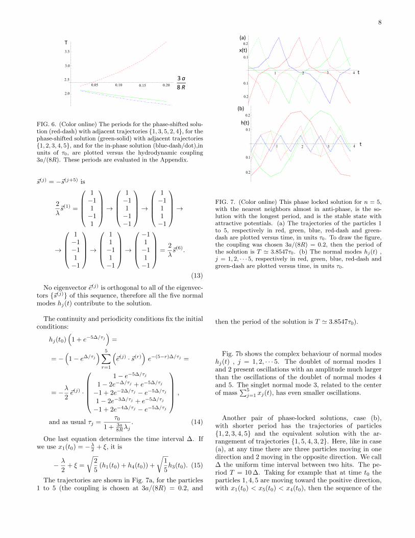
FIG. 6. (Color online) The periods for the phase-shifted solu-tion (red-dash) with adjacent trajectories {1, 3, 5, 2, 4}, for thephase-shifted solution (green-solid) with adjacent trajectories{1, 2, 3, 4, 5}, and for the in-phase solution (blue-dash/dot),inunits of τ0, are plotted versus the hydrodynamic coupling3a/(8R). These periods are evaluated in the Appendix.

~s(j) = −~s(j+5) is

2

λ~s(1) =

1−11−11

→

1−11−1−1

→

1−111−1

→

→

1−1−11−1

→

11−11−1

→−11−11−1

=2

λ~s(6).

(13)

No eigenvector ~e(j) is orthogonal to all of the eigenvec-tors {~s(j)} of this sequence, therefore all the five normalmodes hj(t) contribute to the solution.

The continuity and periodicity conditions fix the initialconditions:

hj(t0)(

1 + e−5∆/τj)

=

= −(

1− e∆/τj) 5∑r=1

(~e(j) · ~s(r)

)e−(5−r)∆/τj =

= −λ2~e(j) ·

1− e−5∆/τj

1− 2e−∆/τj + e−5∆/τj

−1 + 2e−2∆/τj − e−5∆/τj

1− 2e−3∆/τj + e−5∆/τj

−1 + 2e−4∆/τj − e−5∆/τj

,

and as usual τj =τ0

1 + 3a8Rλj

. (14)

One last equation determines the time interval ∆. Ifwe use x1(t0) = −λ2 + ξ, it is

− λ

2+ ξ =

√2

5(h1(t0) + h4(t0)) +

√1

5h3(t0). (15)

The trajectories are shown in Fig. 7a, for the particles1 to 5 (the coupling is chosen at 3a/(8R) = 0.2, and

0.2

0.1

0.1

0.2

321 4

x(t)

t

(a)

t

h(t)

(b)0.2

0.1

0.1

0.2

1 2 3 4

FIG. 7. (Color online) This phase locked solution for n = 5,with the nearest neighbors almost in anti-phase, is the so-lution with the longest period, and is the stable state withattractive potentials. (a) The trajectories of the particles 1to 5, respectively in red, green, blue, red-dash and green-dash are plotted versus time, in units τ0. To draw the figure,the coupling was chosen 3a/(8R) = 0.2, then the period ofthe solution is T ' 3.8547τ0. (b) The normal modes hj(t) ,j = 1, 2, · · · 5, respectively in red, green, blue, red-dash andgreen-dash are plotted versus time, in units τ0.

then the period of the solution is T ' 3.8547τ0).

Fig. 7b shows the complex behaviour of normal modeshj(t) , j = 1, 2, · · · 5. The doublet of normal modes 1and 2 present oscillations with an amplitude much largerthan the oscillations of the doublet of normal modes 4and 5. The singlet normal mode 3, related to the centerof mass

∑5j=1 xj(t), has even smaller oscillations.

Another pair of phase-locked solutions, case (b),with shorter period has the trajectories of particles{1, 2, 3, 4, 5} and the equivalent solution with the ar-rangement of trajectories {1, 5, 4, 3, 2}. Here, like in case(a), at any time there are three particles moving in onedirection and 2 moving in the opposite direction. We call∆ the uniform time interval between two hits. The pe-riod T = 10 ∆. Taking for example that at time t0 theparticles 1, 4, 5 are moving toward the positive direction,with x1(t0) < x5(t0) < x4(t0), then the sequence of the

9

vectors {~s(j)}, with j = 1, · · · , 10 , ~s(j) = −~s(j+5) is

2

λ~s(1) =

1−1−111

→

1−1−1−11

→

11−1−11

→

→

11−1−1−1

→

111−1−1

→−111−1−1

=2

λ~s(6).

(16)

As before, the continuity and periodicity conditions fixthe initial conditions:

hj(t0)(

1 + e−5∆/τj)

=

= −(

1− e∆/τj) 5∑r=1

(~e(j) · ~s(r)

)e−(5−r)∆/τj =

= −λ2~e(j) ·

1− e−5∆/τj

1− 2e−3∆/τj + e−5∆/τj

1− 2e−∆/τj + e−5∆/τj

−1 + 2e−4∆/τj − e−5∆/τj

−1 + 2e−2∆/τj − e−5∆/τj

,

and as usual τj =τ0

1 + 3a8Rλj

. (17)

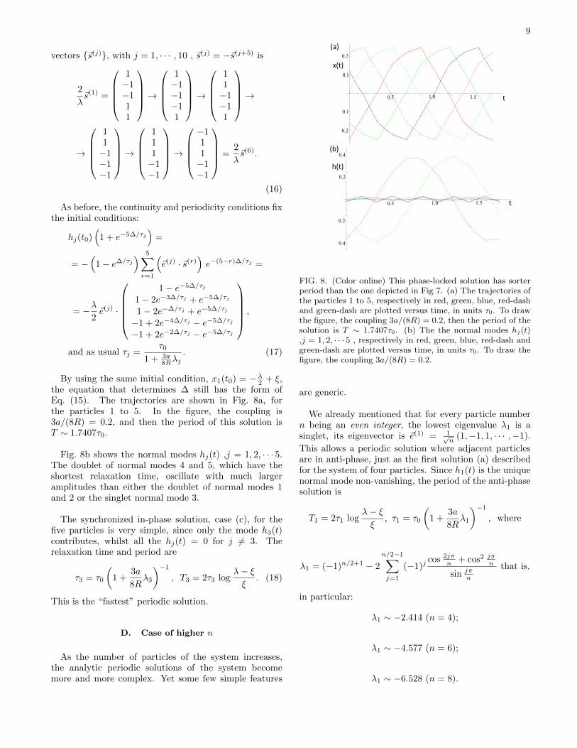
By using the same initial condition, x1(t0) = −λ2 + ξ,the equation that determines ∆ still has the form ofEq. (15). The trajectories are shown in Fig. 8a, forthe particles 1 to 5. In the figure, the coupling is3a/(8R) = 0.2, and then the period of this solution isT ∼ 1.7407τ0.

Fig. 8b shows the normal modes hj(t) ,j = 1, 2, · · · 5.The doublet of normal modes 4 and 5, which have theshortest relaxation time, oscillate with much largeramplitudes than either the doublet of normal modes 1and 2 or the singlet normal mode 3.

The synchronized in-phase solution, case (c), for thefive particles is very simple, since only the mode h3(t)contributes, whilst all the hj(t) = 0 for j 6= 3. Therelaxation time and period are

τ3 = τ0

(1 +

3a

8Rλ3

)−1

, T3 = 2τ3 logλ− ξξ

. (18)

This is the “fastest” periodic solution.

D. Case of higher n

As the number of particles of the system increases,the analytic periodic solutions of the system becomemore and more complex. Yet some few simple features

0.2

0.1

0.2

0.1

0.5 1.0 1.5

x(t)

t

(a)

0.2

0.5

0.2

0.4

1.0 1.5

h(t)

(b)0.4

t

FIG. 8. (Color online) This phase-locked solution has sorterperiod than the one depicted in Fig 7. (a) The trajectories ofthe particles 1 to 5, respectively in red, green, blue, red-dashand green-dash are plotted versus time, in units τ0. To drawthe figure, the coupling 3a/(8R) = 0.2, then the period of thesolution is T ∼ 1.7407τ0. (b) The the normal modes hj(t),j = 1, 2, · · · 5 , respectively in red, green, blue, red-dash andgreen-dash are plotted versus time, in units τ0. To draw thefigure, the coupling 3a/(8R) = 0.2.

are generic.

We already mentioned that for every particle numbern being an even integer, the lowest eigenvalue λ1 is asinglet, its eigenvector is ~e(1) = 1√

n(1,−1, 1, · · · ,−1).

This allows a periodic solution where adjacent particlesare in anti-phase, just as the first solution (a) describedfor the system of four particles. Since h1(t) is the uniquenormal mode non-vanishing, the period of the anti-phasesolution is

T1 = 2τ1 logλ− ξξ

, τ1 = τ0

(1 +

3a

8Rλ1

)−1

, where

λ1 = (−1)n/2+1 − 2

n/2−1∑j=1

(−1)jcos 2jπ

n + cos2 jπn

sin jπn

that is,

in particular:

λ1 ∼ −2.414 (n = 4);

λ1 ∼ −4.577 (n = 6);

λ1 ∼ −6.528 (n = 8).

10

This anti-phase solution is the periodic solution with thelongest period, for every even n.

We also mentioned that for every n being odd integern ≥ 5, the lowest eigenvalue λ1 is a doublet. Theperiodic solution with the longest period is analogous tothe solution (a) for the system of five particles. Thatis a pair of equivalent solutions where a sequence oftrajectories are time shifted by a uniform time interval.For n = 7 the pair of sequences is {1, 3, 5, 7, 2, 4, 6}and {1, 6, 4, 2, 7, 5, 3}. One may notice that if n >> 1,adjacent particles are time shifted by almost half period,that is are approximately in anti-phase. Thus thedistinction between even and odd number n decreases,as n increases.

E. Simulations

To verify which of the analytical solutions is the dy-namical steady state, we resorted to numerical integra-tion. Two different codes have been developed.

Firstly we solved the coupled system of Eq.2 whichcorresponds to the tangential motion, using the solverode113 of matlab, which implements the Adams-Bashforth-Moulton multi-step (i.e. timestep optimizing)method. We used the event handling facility integratedinto all matlab’s ode solvers to intercept the instant oftime at which any one of the particles hits the switchposition. As a stabilizing measure, we imposed that ata “hit” all particles which are in the range of δs fromtheir switches are considered to have hit their target andconsequently their centers of force switch their positions;several values in the interval 10−8 λ ≤ δs ≤ 10−5 λ havebeen used with no substantial difference on the results.

Secondly, a different code described in [3, 4, 14] withfixed timestep, is also used, enabling testing in the ab-sence of noise but also the robustness at finite tempera-ture. As well as exploring noise, this Brownian Dynamics(BD) code solves a model which is very close to the ex-perimental condition [4]: the colloidal particles are free tomove in a two dimensional environment, and the tangen-tial and normal forces can be set independently at differ-ent stiffnesses. Finally, experiments typically work at afinite sampling rate, and this can be mimicked closely inthe fixed-timestep BD code as was discussed in previousstudy [3].

The numerical solution (both the simulation ap-proaches described above) show the remarkable resultthat for every particle number n and every initial condi-tion, the system evolves to a synchronized configurationcorresponding to the periodic solution with the longestperiod (for the case of positive trap stiffness κ > 0 dis-cussed up to here). If such a configuration is a pair ofequivalent solutions, as it happens for odd n ≥ 5, thesynchronization occurs on either one of the pair. Thesefindings also agree with the experiment in [4].

x(t)

t

FIG. 9. (Color online) Trajectory of a driven oscillator withrepulsive driving force, uncoupled to other oscillators. Notethe increase in velocity between switch positions, characteris-tic of the motion with potentials of negative stiffness.

Another result of the extensive numerical solutions isthat we never observe different solutions from the casesthat were investigated analytically (in principle, we couldnot have ruled out the presence of much more complexand less symmetric solutions).

V. REPULSIVE POTENTIAL

It is interesting to consider a harmonic repulsive po-tential, κ < 0, acting on the colloidal spheres. This maybe realized experimentally by tailoring an appropriatepotential landscape with time-sharing or holographicaloptical traps. Then the synchronization of the systemof oscillating particles due to the hydrodynamicalinteraction still occurs, but on a periodic configurationdifferent from the one observed in the attractive case.With minimal changes from the previous analysis wecan describe the periodic solutions occurring in the caseof repulsive harmonic potentials. Again the numericalsimulations of this case confirm that the systems con-verge onto one of the analytical solutions, and in thiscase it is one with short period.

With negative stiffness, if we ignore the hydrody-namic coupling, a particle moves toward the pos-itive x axis according to the differential equationγ0 x(t) +κ

(x(t) + λ

2

)−f(x) = 0, where now κ < 0 is the

stiffness of the repulsive harmonic force, τ0 = γ0/|κ|, fis a stochastic force due to thermal agitation of the fluid,which will be ignored in the analysis of the deterministicsystem. In this case, the motion is exponentially accel-erated until the particle reaches the position λ

2 − ξ. Atthat time the center of the repulsive harmonic potentialmoves from the position −λ2 to λ

2 . The particle inverts

its motion until it reaches the position −λ2 + ξ whenthe potential jumps again. The resulting oscillatorymotion for a single particle (or one in a non-coupled sys-tem), neglecting the stochastic force, is depicted in Fig. 9.

The period T0 of these uncoupled oscillations is

11

T0 = 2τ0 log λ−ξξ . The oscillatory motion is similar to

the attractive potential case, shown in Fig. 1, except forthe concavity.

One may repeat the analysis of the attractive case, andobtain the linear deterministic system, valid in a timeinterval between two hits:(

I +3a

8RCn

)(~x(t)− ~s)− τ0

d

dt~x(t) = 0, τ0 =

γ0

|κ|,

(19)

where ~x(t) is the n component vector of the (local) posi-tion of the particles, ~s is the n component vector of the(local) position of the minima of the repulsive potentialproper for such time interval (opposite of the previouscase), Cn is the same real symmetric circulant matrixof order n, given in eq.(3). We again define the normalmodes hj(t) =

(~e(j), ~x(t)

)and their decoupled equations:

hj(t)−(~e(j) · ~s

)− τj

d

dthj(t) = 0, τj =

τ0

1 + 3a8Rλj

.

(20)

They differ from the previous equations (5) only forthe sign of the time evolution. It follows that theset of periodic solutions, described in the previousanalysis for the attractive traps, still exist in thepresent case of repulsive traps, with the same periods.Only the shape of the trajectories is affected by re-placing diverging exponential in place of converging ones.

Fig. 10a and Fig. 10b are examples of this point,when compared with the Fig. 3a and Fig. 3b. Weplotted the phase-locked solution for three particles inthe repulsive case. Fig. 10a shows the trajectories ofthe three particles as function of time, for one periodT = 6∆. Fig. 10b plots the normal modes h1(t), h2(t)and h3(t), again for one period. The oscillations of thepair of normal modes corresponding to the degenerateeigenvalue have an amplitude much bigger then theoscillations of the normal mode h1(t). Remarkably, thesimulations show that in the case of repulsive traps it isthis periodic solution, the one with the shortest period,which is the stable asymptotic synchronization for thesystem.

With systems of higher n, we have observed in thenumerical simulations that again on switching from at-tractive to repulsive traps the stable solution ceases to bethat with longest period. Instead, the system convergesonto one of the solutions with shortest period. However,as is clear by observing the sequence of solution peri-ods T calculated for the cases (n = 4 or n = 5), whilethere is a clearly separate largest T , there are varioussolutions with small T . We have tested numerical solu-tions in the physically realistic parameter space, usingthe two numerical approaches outlined in section IV E:the ODE solver with the “strong” tangential motion con-straint converges to the shortest period solution, whereas

x(t)

(a)

t

0.2

0.1

0.5

0.1

0.2

1.0 1.5 2.0

h(t)

(b)

t

0.2

0.1

0.1

0.2

0.5 1.0 1.5 2.0

FIG. 10. (Color online) (a) The trajectories for the the phase-locked solution for three particles in the repulsive case areplotted versus time, in units τ0. (b) The normal modes h1(t)in red-dash, h2(t) in green-solid, h3(t) in blue dash/dot areplotted versus time, in units of τ0.

the Brownian Dynamics simulation with the weaker “har-monic” constraint converges to one of the shorter periodsolutions, but not always the shortest one. This will beexplored further in future work; our current understand-ing is that the system with repulsive potentials convergesto one of the solutions with shorter periods, and thatwhen there are various periods grouped close togetherthe details of the system play a strong role in selectingbetween these.

VI. CONCLUSION

The model studied in this paper has several unusualfeatures. Most studies on synchronization show that it isa threshold process: it occurs when the coupling amongthe oscillators is strong enough or when increasing thenumber of oscillators, a large fraction synchronize toa common frequency [15]. In contrast, in the presentmodel, where we studied the deterministic systemwithout stochastic forces, we find no threshold. Synchro-nization occurs for any strength of the hydrodynamiccoupling, that is any value of a/R, and any number ofoscillators.Most models on synchronization are described bynon-linear differential equations where a very limitedprogress is achieved analytically, whereas the presentmodel is piece-wise linear and all periodic solutions maybe derived.Numerical solutions in the case of attractive harmonic

12

potentials clearly show the synchronization to the peri-odic solution with the longest period, for any number ofparticles. In the case of repulsive harmonic potentials,numerical simulations show the synchronization to thethe pair of phase locked solutions in the case of threeparticles. We have not performed a stability analysisabout the periodic solutions, but there is no reasonto expect disagreement with the results of numericalsimulations. This change of the asymptotic solutionwith the change of curvature of the potential hadalready been shown numerically for a linear chain in [12].The analytical framework developed here adequatelydescribes experiments on systems of colloidal particleswith moving optical traps [4].

VII. APPENDIX

In the case of three particles, with attractive harmonictraps, the initial conditions for the normal modes, forperiodic phase-locked solutions are given in the eqs.(9).We supplement them with an initial condition:

x1(t0) =1√3h1(t0)− 2√

6h3(t0) = −λ

2+ ξ,

and obtain an equation that determines ∆:

λ

6

(1− e−∆/τ1

)(e−2∆/τ1 − e−∆/τ1 + 1

)(1 + e−3∆/τ2

)+λ

3

(1− e−∆/τ2

)(e−2∆/τ2 + 2e−∆/τ2 + 1

)(1 + e−3∆/τ1

)=

(λ

2− ξ)(

1 + e−3∆/τ1)(

1 + e−3∆/τ2). (21)

Furthermore, τ0/τ1 + 2τ0/τ2 = 3, since λ1 + 2λ2 = 0. Letus define:

x = e−∆/τ0 , p1 =τ0τ1< 1, p2 =

τ0τ2> 1, p1 + 2p2 = 3,

then Eq.(21) may be rewritten in the simpler form:

λ

3

[− xp1 + x2p1 − x3p1 + xp2

(1 + xp1 − x2p1 + 2x3p1

)+

+x2p2(−2− xp1 + x2p1 − 3x3p1

) ]+

+ ξ(1 + x3p1

) (1− xp2 + x2p2

)= 0. (22)

If we choose the coupling strength 3a/(8R) =√

3/5, wehave p1 = 0.8 and p2 = 1.1. The further behaviour of ∆as function of λ/ξ is depicted in Fig. 4.If we further choose ξ = λ/4, then eq.(21) implies x ∼0.70701565, that is:

∆

τ0= − log x ∼ 0.346702, T = 6∆ = −6τ0 log x .

For the case of five particles with attractive traps,Fig. 6 shows the period T in units of τ0 for the phase-shifted solution with adjacent trajectories {1, 3, 5, 2, 4},the period of the phase-shifted solution with adjacenttrajectories {1, 2, 3, 4, 5}, and the in-phase solution, ver-sus the hydrodynamic coupling 3a/(8R), while we fixedλ = 1, ξ = 0.25. In the limit of vanishing coupling, thethree curves converge to T = 2τ0 log(λ−ξ)/ξ ∼ 2.1972 τ0.

AcknowledgmentsWe are grateful for many discussions with Filippo deLillo, Nicolas Bruot and Romain Lhermerout.

[1] S. Gueron, K. Levit-Gurevich, N. Liron, and J. Blum,Proc. Natl. Acad. Sci. 94, 6001 (1997).

[2] R. Golestanian, J. Yeomans, and N. Uchida, Soft Matter7, 3074 (2011).

[3] J. Kotar, M. Leoni, B. Bassetti, M. Cosentino Lago-marsino, and P. Cicuta, Proc. Natl. Acad. Sci. 107, 7669(2010).

[4] L. Damet, G. M. Cicuta, J. Kotar, M. Cosentino Lago-marsino, and P. Cicuta, arXiv:1110.1526 (2011).

[5] J. Happel and H. Brenner, Low Reynolds Number Hydro-dynamics: with special applications to particulate media(Kluwer, New York, 1983).

[6] R. J. Hunter, Foundations of Colloid Science (OxfordUniversity Press, New York, 1981).

[7] E. Lauga and T. R. Powers, Rep. Prog. Phys. 72, 096601(2009).

[8] M. Polin, D. Grier, and S. Quake, Phys. Rev. Lett. 96,088101 (2006).

[9] R. Di Leonardo, S. Keen, R. Leach, C. D. Saunter, G. D.Love, G. Ruocco, and M. J. Padgett, Phys. Rev. E 76,061402 (2007).

[10] G. M. Cicuta, J. Kotar, A. T. Brown, J. Noh, and P. Ci-cuta, Phys. Rev. E 81, 051403 (2010).

[11] M. Cosentino Lagomarsino, P. Jona, and B. Bassetti,Phys. Rev. E 68, 021908 (2003).

[12] C. Wollin and H. Stark, Eur. Phys. J. E 34, 42 (2011).[13] N. Uchida and R. Golestanian, Phys. Rev. Lett. 106,

058104 (2011).[14] D. L. Ermak and J. A. McCammon, J. Chem. Phys. 69,

1352 (1978).[15] A. Pikovsky, M. Rosenblum, and J. Kurths, Synchoniza-

tion (Cambridge Univ. Press, Cambridge (U.K.), 2001).