Significance analysis of time-series transcriptomic data: A methodology that enables the...

ARTICLE

Significance Analysis of Time-SeriesTranscriptomic Data: A Methodology That Enablesthe Identification and Further Exploration of theDifferentially Expressed Genes at Each Time-Point

Bhaskar Dutta,1 Robert Snyder,1 Maria I. Klapa1,2

1Metabolic Engineering and Systems Biology Laboratory, Department of Chemical and

Biomolecular Engineering, University of Maryland, College Park, Maryland;

telephone: 301-405-1320; fax: 301-405-0523; e-mail: [email protected] Engineering and Systems Biology Laboratory, Institute of Chemical Engineering

and High Temperature Chemical Processes (ICE-HT), Foundation for Research and

Technology-Hellas (FORTH), Patras GR-26504, Greece

Received 4 August 2006; accepted 7 March 2007

Published online 26 March 2007 in Wiley InterScience (www.interscience.wiley.com)
. DOI 10.1002/bit.21432
ABSTRACT: Time-series transcriptional profiling experi-ments are becoming increasingly popular, in light of theabundance of information regarding a biological system’sregulation that they are expected to reveal. However, iden-tification of differentially expressed genes as a function oftime and comparison between physiological states based onthe genes’ variability in significance level over time remainintriguing tasks, due to certain limitations in the currentlyavailable algorithms. Based on the principles of significanceanalysis of microarrays (SAM) method, we developed analgorithm that allows for the identification of the differen-tially expressed genes at each time-point of a time sequence,using a common reference distribution and significancethreshold for all time-points. These results are furtherexplored in a systematic way to extract information about(a) individual gene and gene class variability in significancelevel with time, (b) gene and time-point correlation based on(a), and (c) gene class comparison based on (a). All algo-rithms have been programmed in C language in the form offour executable files for both Windows and Macintoshplatforms under the overall name MiTimeS. MiTimeSwas validated in the context of real transcriptomic data. Itenables the extraction of biologically relevant informationfrom the dynamic transcriptomic profiles currently unno-ticed from the available algorithms. The applicability ofMiTimeS is not limited to transcriptomic data, but it couldbe accordingly used for the analysis of dynamic data fromother cellular fingerprints.

Biotechnol. Bioeng. 2007;98: 668–678.

� 2007 Wiley Periodicals, Inc.

Correspondence to: M.I. Klapa

Contract grant sponsor: US NSF

Contract grant number: MCB-0331312

This article contains Supplementary Material available via the Internet at http://

www.interscience. wiley.com/jpages/0006-3592/suppmat.

668 Biotechnology and Bioengineering, Vol. 98, No. 3, October 15, 2007

KEYWORDS: hypothesis testing; dynamic–omic profiling;highthroughput analysis; time-point comparison; systemsbiology; bioinformatics

Introduction

In our effort to identify the mechanisms and networksunderlying cellular function, biological studies havetraditionally involved the perturbation of a cellular systemin multiple ways and the monitoring of its response throughvarious markers. Prior to the genomic revolution, thesemarkers were mainly macroscopic. The high-throughputpost-genomic era provided the tools, DNA microarrays(Brown and Botstsein, 1999; Schena et al., 1995) being themost often utilized among them, to also monitorsimultaneously a great number of molecular markers (Klapaand Quackenbush, 2003). The computational problems,therefore, that biology has often to solve concern theidentification of differentially expressed markers due to theapplied perturbation(s). In the case of transcriptionalprofiling, in particular, these problems refer to theidentification of differentially expressed genes betweentranscriptional profile populations representing differentsets of physiological conditions. There are two types ofexperiments: ‘‘snapshot’’ and ‘‘time-series’’. In the first type,

� 2007 Wiley Periodicals, Inc.

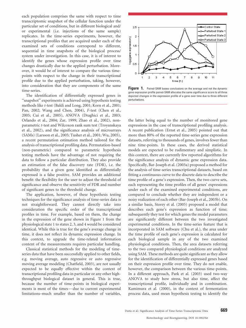
Figure 1. Paired-SAM bases conclusions on the average and not the dynamic

gene expression profile paired-SAM allocates the same significance score to all three

depicted changes in the expression profile of a gene over time due to three different

perturbations.

each population comprises the same with respect to timetranscriptomic snapshot of the cellular function under theparticular set of conditions, but in different biological and/or experimental (i.e. injections of the same sample)replicates. In the time-series experiments, however, thetranscriptional profiles that are acquired under each of theexamined sets of conditions correspond to different,sequential in time snapshots of the biological process/system under investigation. In this case, it is of interest toidentify the genes whose expression profile over timechanges drastically due to the applied perturbation. More-over, it would be of interest to compare the various time-points with respect to the change in their transcriptionalprofile due to the applied perturbation, taking, however,into consideration that they are components of the sametime-series.

The identification of differentially expressed genes in‘‘snapshot’’ experiments is achieved using hypothesis testingmethods like t-test (Baldi and Long, 2001; Korn et al., 2001;Pan, 2002; Wang and Chen, 2004), F-test (Chen et al.,2005; Cui et al., 2005), ANOVA (Draghici et al., 2003;Orlando et al., 2004; Zar, 1999; Zhao et al., 2002), non-parametric t-test and Wilcoxon rank sum test (Troyanskayaet al., 2002), and the significance analysis of microarrays(SAMs) (Larsson et al., 2005; Tusher et al., 2001; Wu, 2005),a recent permutation estimation method tailored for theanalysis of transcriptional profiling data. Permutation-based(non-parametric) compared to parametric hypothesistesting methods have the advantage of not requiring thedata to follow a particular distribution. They also providean estimation of the false discovery rate (FDR), i.e. theprobability that a given gene identified as differentiallyexpressed is a false positive. SAM provides an additionalbenefit: the flexibility for the user to adjust the threshold ofsignificance and observe the sensitivity of FDR and numberof significant genes to the threshold change.

The application, however, of these hypothesis testingtechniques for the significance analysis of time-series data isnot straightforward. They cannot directly take intoconsideration the specific order of the transcriptionalprofiles in time. For example, based on them, the changein the expression of the gene shown in Figure 1 from thephysiological state 1 to states 2, 3, and 4 would be consideredidentical. While this is true for the gene’s average change intime, it does not reflect its dynamic expression change. Inthis context, to upgrade the time-related informationcontent of the measurements requires particular handling.

Classical statistical methods for the modeling of time-series data that have been successfully applied to other fields,e.g. moving average, auto regressive or auto regressivemoving average modeling (Chatfield, 2003), are not usuallyexpected to be equally effective within the context oftranscriptional profiling data in particular or any other high-throughput biological dataset in general. This is true,because the number of time-points in biological experi-ments is most of the times—due to current experimentallimitations–much smaller than the number of variables,

Du

the latter being equal to the number of monitored geneexpressions in the case of transcriptional profiling analysis.A recent publication (Ernst et al., 2005) pointed out thatmore than 80% of the reported time-series gene expressiondatasets, referring to thousands of genes, involves fewer thannine time-points. In these cases, the derived statisticalmodels are expected to be rudimentary and simplistic. Inthis context, there are currently few reported algorithms forthe significance analysis of dynamic gene expression data.Specifically, Bar-Joseph et al. (2003a) proposed amethod forthe analysis of time-series transcriptional datasets, based onfitting a continuous curve to the discrete data to describe thetime profile of a gene’s expression. Then, the two curve sets,each representing the time profiles of all genes’ expressionsunder each of the examined experimental conditions, arecompared to conclude whether they are independent or anoisy realization of each other (Bar-Joseph et al., 2003b). Ona similar basis, Storey et al. (2005) proposed a model thatdescribes each gene’s expression as function of time;subsequently they test for which genes the model parametersare significantly different between the two investigatedexperimental conditions. In the time-series feature that isincorporated in SAM software (Chu et al.), the area underthe time profile of each gene’s expression is calculated foreach biological sample in any of the two examinedphysiological conditions. Then, the area datasets referringto the two compared physiological conditions are analyzedusing SAM. Thesemethods are quite significant as they allowfor the identification of differentially expressed genes basedon their expression profile over time. They do not enable,however, the comparison between the various time-points.In a different approach, Park et al. (2003) used two-wayANOVA to study how stress, but also time, affect thetranscriptional profile, individually and in combination.Kamimura et al. (2000), in the context of fermentationprocess data, used mean hypothesis testing to identify the

tta et al.: Significance Analysis of Time-Series Transcriptomic Data 669

Biotechnology and Bioengineering. DOI 10.1002/bit

most discriminatory variables and time windows. Liu et al.(2005), on the other hand, compared the time-points of aplant growth process directly through the SAM-identifieddifferentially expressed genes at each time-point, consider-ing, however, each time-point as an independent ‘‘snap-shot’’ experiment. Consequently, each SAM analysis wasconducted independently, without using a commonreference for normalization among the time-points.

In this paper, we present an SAM-based algorithm thatenables the identification of the differentially expressedgenes at each time-point of a time sequence, taking,however, into consideration that they correspond tosequential snapshots of the same biological process. Thisis achieved by comparing the gene expression profile of alltime-points with a common reference distribution and byidentifying the differentially expressed genes at each time-point based on a common threshold of significance. Theextracted information is further explored to obtain insightabout the regulation of gene networks. No similar type oftime-series data analysis exists currently in the literature.Specifically, we present a systematic methodology thatallows for (a) deducing and appropriately storing theindividual gene and gene class variability in significancelevel with time and (b) comparing genes, gene classes andtime-points based on (a). The derived information isexpected to unravel significant characteristics of a biologicalsystem’s dynamic response to particular perturbation(s).This is demonstrated in the last section of the present paperin the context of a real time-series transcriptomic dataset(see also Dutta, 2007; Kanani, 2007). The applicability of theproposed algorithm and subsequent data analysis metho-dology is not limited to transcriptomic data, but they couldbe accordingly applied to time-series high-throughputbiological data of any other type (e.g. proteomic ormetabolomic), as it has been demonstrated in Dutta(2007) and Kanani (2007).

Materials and Methods

Experimental Design/Dataset

The transcriptional profiling data that we used tovalidate the presented analytical methodology was obtainedfrom a time-series experiment monitoring the short-termresponse of Arabidopsis thaliana liquid culture system toelevated CO2, described in great detail in Dutta (2007) andKanani (2007). Specifically, we grew two sets of A. thaliana(Columbia strain) liquid cultures (20 liquid cultures each)for 12 days in Gamborg media and sucrose (Kanani et al.,2005) at constant temperature (238C) and light (80–100mmol/m2 s). On the 13th day, the CO2 concentration in thegrowth environment of one of the two culture sets wasincreased to 1%. In the rest of the paper, this set will bereferred as ‘‘perturbed’’ to differentiate it from the ‘‘control’’set. At time zero, i.e. just before the initiation of theperturbation, we harvested four liquid cultures from each


culture set to be used as the reference of the plant growthup to that stage. Subsequently, we harvested twoliquid cultures (each comprising �100 plants) fromeach experimental set at 1, 3, 6, 9, 12, 18, 24, and 30 hafter the initiation of the perturbation. Each of theharvested cultures (40 in total) was subjected to mRNAextraction followed by hybridization (Kim et al., 2003) onfull-genome cDNA microarrays prepared at TIGR (Kimet al., 2003).

Microarray Data Analysis

Image processing and data normalization was carried outusing TIGR Spotfinder (V2.2.4) and MIDAS (V2.19) (Saeedet al., 2003), respectively. The normalization involved locallyweighted scatterplot smoothing regression (LOWESS)(smooth parameter: 0.33; reference: Cy3), variance regular-ization (reference: Cy3) and ‘‘flip-dye’’ data consistencytrim (data trim option: SD cut; cross log ratio data keeprange: �2 SD). Following normalization (Dutta, 2007;Kanani, 2007), we estimated the geometric mean of thetranscriptional profiles of the biological replicates (four attime 0 h or two at subsequent time-points) that had beenharvested at the same time-point to represent thetranscriptional state of each culture set at that time-point.Subsequently, we normalized the transcriptional profiles ofthe eight time-points at each of the control and perturbedconditions with respect to the transcriptional profile of the0 h in the corresponding culture set (Dutta, 2007; Kanani,2007). Paired-SAM analysis of the final 16 (8 ‘‘control’’ and8 ‘‘perturbed’’—time 0 h excluded) transcriptional profileswas performed using TIGR MeV (Saeed et al., 2003).Analysis of the 16 transcriptional profiles based on themethodology described in this paper was performed usingthe software MiTimeS, which has been programmed by theauthors’ team in C language. MiTimeS can run on bothWindows and Macintosh platforms and is available (for freeto academic users) upon request.

Results and Discussion

SAM-Based Algorithm for the Identification ofDifferentially Expressed Genes at Each Time-Point

SAM identifies the genes that are differentially expressedbetween two experimental groups based on whether thedifference between a gene’s observed (d(i)) and expected(de(i)) ‘‘relative differences’’ is greater than a significancethreshold ‘delta’ (Tusher et al., 2001). Paired-SAM, inparticular, deals with the analyses in which the samplesof the two experimental groups can be paired accordingto the experimental design, time-series analyses being acharacteristic example. In these cases, the ‘‘per pair’’information is used in the estimation of the relative

DOI 10.1002/bit

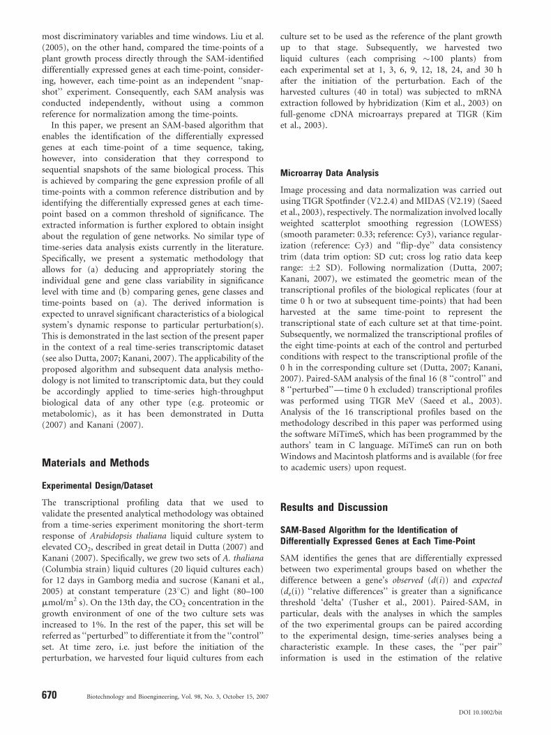
Figure 2. Schematic representation of the presented time-dependent modified

SAM algorithm d(i), de(i), dt(i), NT, NG depict, respectively, the observed relative

difference of gene i based on the SAM definition as described in Eq. (1), the expected

relative difference of gene i based on the SAM definition as described in the text, the

observed relative difference of gene i at time-point t according to the proposed

algorithm as described in Eq. (2), the total number of time-points and the total number

of gene expressions included in the significance analysis.

differences d(i) and de(i). Specifically, d(i) is defined asfollows:

dðiÞ ¼ X1ðiÞ � X2ðiÞSðiÞ þ S0

(1)

where XkðiÞ represents the mean expression of gene i inexperimental group k (k¼ 1 or 2); S(i) represents thestandard deviation of the per pair differences in expressionof gene i between the two experimental groups; S0 depicts apositive fudge factor used to eliminate numerical biases atlow values of S(i). The observed scores are ranked indecreasing order and d(i) corresponds to the ith ranked geneof the distribution. de(i) is also estimated from Eq. (1), butin this case the samples are multiple times divided into twogroups of the same size as the original by random samplingpermutations. For each permutation, the calculated basedon Eq. (1) gene scores are also ranked in decreasing order.The average of the scores in the ith position among allpermutations is considered as de(i). Finally, the twodistributions are plotted in a quantile–quantile plot andthe genes whose absolute difference between the observedand the expected scores is larger than delta are identified asdifferentially expressed. FDR is estimated based on twocuttoffs defined by the minimum and maximum (leastnegative) d(i) values from the cluster of positively andnegatively significant genes, respectively (Tusher et al.,2001). For each permutation of the expected distribution,the number of genes ‘‘laying outside’’ the cutoff region isdetermined; the median of this number over all permuta-tions is multiplied by a correction factor to estimate FDR.

Hence, in the case of time-series analysis, SAM identifiesas differentially expressed the genes whose average over timeexpression has changed due to the applied perturbation to agreater than delta extent than what it would have beenanticipated due to random differences among samples, thelatter being quantified by the relative expected differencedistribution, de. In the context of this analysis, theexpression of a gene at any time-point is represented byits average expression over all sampled biological andexperimental replicates at this time-point. Following thesame concept, we define as differentially expressed at aparticular time-point the genes whose expression at thistime-point has changed due to the applied perturbation to agreater than delta extent than what it would have beenexpected based on the null distribution de. In this way, weuse the same reference distribution of expected geneexpression differences and the same significance thresholddelta for all time-points, taking inherently into considera-tion that they are part of the same time sequence.Specifically, the ‘‘time-dependent’’ statistic that we proposefor the new algorithm is the observed score of gene i at aparticular time-point t, which is defined based on Eq. (1) asfollows:

dtðiÞ ¼Xt1ðiÞ � Xt

2ðiÞSðiÞ þ S0

(2)

Du

where ðXt1ðiÞ � Xt

2ðiÞÞ represents the difference in theexpression of gene i between the two experimental groupsat time-point t; the rest of the symbols represent the samequantities as in Eq. (1). For each time-point, the distributionof observed scores is separately ranked in the decreasingorder and dt(i) represents the observed score of theith ranked gene at the tth time-point. At a particulartime-point t, gene i is identified as differentially expressed, ifthe absolute difference between its observed score at thistime-point and the ith expected score is larger than delta (seeschematic diagram in Fig. 2).

There have been concerns regarding the use of the sameexpected distribution for each time-point and paired-SAMand to what extent this could lead to high number of false



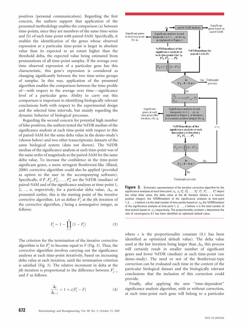
Figure 3. Schematic representation of the iterative corrective algorithm for the

significance analyses at each time-pointD0,Dj, F10 ; F

20 ; . . . ; F

n0 ; F

1j ; F

2j ; . . . ; F

nj depict

the initial delta value, the delta value at the jth iteration (where j a nonzero

positive integer), the %FDR(median) of the significance analysis at time-point

1, 2, . . ., n (where n is the total number of time-points) based onD0, the %FDR(median)

of the significance analysis at time-point 1, 2, . . ., n (where n is the total number of

time-points) based on Dj, respectively. The proportionality constant c determines the

rate of convergence; 0.1 has been identified as optimized default value.

positives (personal communication). Regarding the firstconcern, the authors support that application of thepresented methodology enables the comparison (a) betweentime-points, since they are members of the same time-seriesand (b) of each time-point with paired-SAM. Specifically, itenables the identification of the genes whose observedexpression at a particular time-point is larger in absolutevalue than its expected to an extent higher than thethreshold delta, the expected value being estimated frompermutations of all time-point samples. If the average overtime observed expression of a particular gene has thischaracteristic, this gene’s expression is considered aschanging significantly between the two time-series groupsof samples. In this way, application of the presentedalgorithm enables the comparison between the time-profileof—with respect to the average over time—significancelevel of a particular gene. Ability to carry out thiscomparison is important in identifying biologically relevantconclusions both with respect to the experimental designand the selected time intervals, but mainly regarding thedynamic behavior of biological processes.

Regarding the second concern for potential high numberof false positives, the authors tested the %FDRmedian of thesignificance analysis at each time-point with respect to thisof paired-SAM for the same delta value in the demo-study’s(shown below) and two other transcriptomic datasets of thesame biological system (data not shown). The %FDRmedian of the significance analysis at each time-point was ofthe same order of magnitude as the paired-SAM for the samedelta value. To increase the confidence in the time-pointsignificant genes, a more stringent Bonferroni-like (Bland,2000) corrective algorithm could also be applied (providedas option to the user in the accompanying software).Specifically, if F;F1

0 ;F20 ; . . . ;F

n0 are the %FDR (median) of

paired-SAM and of the significance analyses at time-point 1,2,. . ., n, respectively, for a particular delta value, D0, aspresented earlier, this is the starting point of the iterativecorrective algorithm. Let us define F0

j at the jth iteration ofthe corrective algorithm, j being a nonnegative integer, asfollows:

F0j ¼ 1�

Yni¼1

ð1� FijÞ (3)

The criterion for the termination of the iterative correctivealgorithm is for F0

j to become equal to F (Fig. 3). Thus, thecorrective algorithm involves carrying out the significanceanalyses at each time-point iteratively, based on increasingdelta value at each iteration, until the termination criterionis satisfied (Fig. 3). The relative increment in delta at thejth iteration is proportional to the difference between F0

j�1

and F as follows:

Dj

Dj�1¼ 1þ cðF0

j � FÞ (4)


where c is the proportionality constant (0.1 has beenidentified as optimized default value). The delta valueused at the last iteration being larger than D0, this processwill certainly result in smaller number of significantgenes and lower %FDR (median) at each time-point (seedemo-study). The need or not of the Bonferroni-typecorrection can be evaluated each time in the context of theparticular biological dataset and the biologically relevantconclusions that the inclusion of this correction couldprovide.

Finally, after applying the new ‘‘time-dependent’’significance analysis algorithm, with or without correction,at each time-point each gene will belong to a particular

DOI 10.1002/bit

significance level. The latter might be different from thesignificance level in which the gene is classified based onpaired-SAM. In subsequent section, we will discuss somecharacteristic cases of this difference. The results of the newalgorithm could be stored in a matrix, which we accordinglycalled time-dependent significance matrix (TDSM). TDSMhas as many rows as the number of genes (NG) and as manycolumns as the number of time-points (NT). The (i, j)thelement of TDSM is equal to þ1, 0, �1, depending onwhether the ith gene’s change in expression between the twoexperimental groups at time-point j has been, respectively,identified as positively, non or negatively significant.Augmented TDSM (A-TDSM) comprises one additionalcolumn that corresponds to the significance level of thegenes based on paired-SAM.

Clearly, if statistical significance is related to biologicalsignificance, the information in TDSM or A-TDSM could bethe basis for data mining to extract time-dependentbiologically relevant conclusions, which would have beenotherwise missed. Obviously, this is true, independent of thealgorithm by which the information in TDSM, i.e. thesignificance level of each gene at each time-point, mighthave been derived. An obvious data mining exploration ofTDSM data would be the clustering of the genes based ontheir significance level profile over time. In the next sections,we present a series of methods that allow for further use ofthe information in TDSM towards the extraction ofsignificant biological conclusions.

Algorithms for Exploring Gene Variability inSignificance Level Over Time to ExtractBiologically Relevant Conclusions

Significance Variability Score

The information in TDSM could be used to rank the genesbased on their variability in significance level over time. Forthis to become possible, the genes’ significance variability(SV) score needs to be estimated; we propose the followingalgorithm:

1. U
se TDSM to construct the significance variabilitymatrix (SVM). SVM should have as many rows as thenumber of genes (NG) and columns by one fewer than thenumber of time-points (NT� 1). The elements of SVMare estimated to reflect the number of ‘‘significancelevels’’ that a gene ascends or descends from one time-point to the next. Specifically, for i¼ 1, 2,. . ., NG andj¼ 2,. . ., NT:
SVM½i; ðj� 1Þ� ¼ TDSM½i; j� � TDSM½i; ðj� 1Þ�j j (5Þ

Clearly, the genes could be also clustered based on theirSVM profile. The genes clustering together would havesimilar dynamic significance profile. In this case, genesremaining in the same significance level over time

Dutta

would be clustered together independent of thesignificance level; the same for genes, which follow theopposite significance level profile with time, if anabsolute distance metric is used. An easy way todetermine the number of the genes in these clustersand focus on a particular cluster of interest is theestimation of their significance variability (SV) score asindicated below.

2. E
stimate the SV score of the ith gene as the average of theith SVM row’s elements:
SVi ¼PNT�1

j¼1 SVM½i; j�NT � 1

ð6Þ

Based on its definition, the SV score could range from 0to 2. The distribution of the genes with respect to their SVscore might reveal significant information about thebiological problem under investigation. For example, thegenes whose SV score is equal to 2 ‘‘fluctuate’’ betweenthe positively and negatively significant levels from onetime-point to the next throughout the entire time period.Determination of the number and type of these genescould prove significant for understanding the response ofthe biological system to the investigated perturbation,but also for correctly selecting the time-points in futureexperiments to capture subtler changes in gene expres-sion. On the other hand, the genes whose SV score isequal to zero belong to the same significance level at allexamined time-points. These are the genes whoseexpression was significantly affected (either positivelyor negatively) or remained (statistically) unaffected bythe investigated biological perturbation. Obviously, thedistribution of all genes around these two numbers (0, 2)will give simple, but strong, indications regarding thetranscriptional response of the system to the examinedperturbation over time. Paired-SAM results are expectedto have stronger similarity to the results of the presentedalgorithm the more the genes with SV score closer to zeroare.

New Metric for Time-Point Correlation

The change in the physiology of a biological system due to aparticular perturbation at two different time-points could beinitially compared with respect to the number of genes ineach significance level. However, two time-points couldcorrespond to the same number of genes in all threesignificance categories, but still not be biologically corre-lated, because each category comprises different genes ateach time-point. Therefore, another metric that takes intoconsideration the number of common genes in each of thesignificance categories should be defined. Of note, thesame correlation metric could also be used if, instead oftime-points, two experimental conditions or two biologicalperturbations are to be compared.

We defined significance correlation matrix (SCM) withrespect to positively, negatively or non-significant genes the

et al.: Significance Analysis of Time-Series Transcriptomic Data 673


NT�NT symmetric matrix, whose elements are estimated asfollows:

SCMk½i; j� ¼

Gik\Gj

kffiffiffiffiffiffiffiffiffiGik�Gj

k

p for i 6¼ j

Gik

Gik

for i ¼ j

8><>:

(7)

where k depicts the significance level with respect to whichthe time-point comparison is performed (for example,k¼ P, N, O or P\N, if the comparison is made with respectto the positively, negatively, non or the union of positivelyand negatively significant, respectively, genes); Gl

k depictsthe number of genes in the kth significance level at thelth time-point, l ¼ 1; 2; . . . ;NT;Gl

k depicts the number ofgenes in the kth significance level only at the lth time-point(i.e. Gl

k \ Gqk ¼ 0 8 q 6¼ l, q¼ 1, 2, . . ., NT). By definition,

the elements of a SCMmay take values between 0 and 1. Twotime-points might be considered strongly correlated if thecorresponding SCM element(s) is(are) larger than a certainvalue-threshold, usually larger than 0.5. In addition, largediagonal element implies that at this time-point the responseof the system to the particular perturbation(s) is largelydifferent than at the rest.

Gene Class Comparison

If (a) particular gene class(es) is(are) of interest, then thematrices described in the above sections should beconstructed to contain only the gene set associated withthis(these) gene class(es); the same analytical methodologiesdescribed above could be used to extract biologicallyrelevant conclusions focused only on this(these) geneclass(es).

In order to identify the gene class(es) that are highlyenriched in significant genes hypergeometric distributioncould be used as follows: let us suppose that the total numberof genes used in the analysis is N and among these n genesare significant at a particular time-point t. In addition, let usassume that among the y genes that have been associatedwith a particular gene class (among allN genes), x have beenidentified as significant at time-point t. For the nullhypothesis H0: gene class i is not significantly enriched andalternate hypothesisH1: gene class i is significantly enriched,the P-value can be computed in the following way:

P ¼Py

i¼xyCðN�yÞ

iCðn�iÞ

NCn(8)

where aCb represents number of ways we can select belements out of a without replacement. If P< 0.05, thengene class i is significantly enriched.

Specifically, matrices corresponding to each (or to theunion of more than one) of the significance levels could beformed; each of the matrices will have as many columns asthe number of the sampled time-points and as many rows asthe number of gene class(es) that are to be investigated (in a


high-throughput unsupervised way, the latter could be allthe gene class(es) that are associated with the gene listunder investigation). The (i, j)th element of a particularsignificance level’s matrix will be equal to the P-value of theith gene class corresponding to jth time time-point.Studying the information in these matrices, it would bepossible to answer a variety of questions regarding theresponse of the various gene class(es) to the appliedperturbation based on their significance level profile overtime.

Another way to identify the gene class(es) highly enrichedin significant genes would be to construct matrices ofnumber of rows and columns equal to number of geneclass(es) and sampled time-points respectively, whose (i, j)thelement of a particular significance level’s matrix will beequal to the percentage of the ith gene class that has beenclassified in the particular significance level at the jth time-point. Analyzing these matrices, for example, it would bepossible to identify all gene class(es) whose more than 50%of the genes have been consistently classified as (positively ornegatively) significant at each time-point.

Demo-Study

The experimental dataset concerns two experimentalconditions (‘‘control’’ and ‘‘perturbed’’ as described inMaterials and Methods section), eight time-points corre-sponding to different growth stages of A. thaliana plantliquid cultures under the two examined conditions, and11,231 genes per transcriptional profile after normalizationand filtering (75% cutoff) as described in Materials andMethods section and (Dutta, 2007; Kanani, 2007). Forgene classification, the gene ontology (GO) categorization ofTM4 MeV software was used. The case-study will be used todemonstrate the range of time-dependent information thatcan be extracted from dynamic transcriptomic data usingthe presented algorithm.

Paired-SAM identified 690 and 372 genes, respectively, aspositively and negatively significant for a threshold (delta)value of 0.9 (Fig. 4A) and 0.47% FDR (median) (Fig. 4B).For the same expected score distribution and delta value, thenumber of genes that were identified as differentiallyexpressed at any time-point by the presented algorithm islarger (Fig. 4A). Figure 4A shows also the number ofsignificant genes at each time-point when the proposedcorrective algorithm was applied. Since in this case the deltavalue used for the significance analyses at each time-point islarger (i.e. 1.3), there is, in average, a 42� 11% decrease inthe number of identified significant genes at each time-point. However, this number is still significantly larger thanthe number of genes identified from paired-SAM. This is anindication that few genes remained in the same significancelevel at the majority of time-points. This is validated fromthe SV score distribution (Fig. 5A). Specifically, among11,231, only 73, 36, and 85 genes, respectively, wereidentified as positively, negatively and non-significant at all

DOI 10.1002/bit

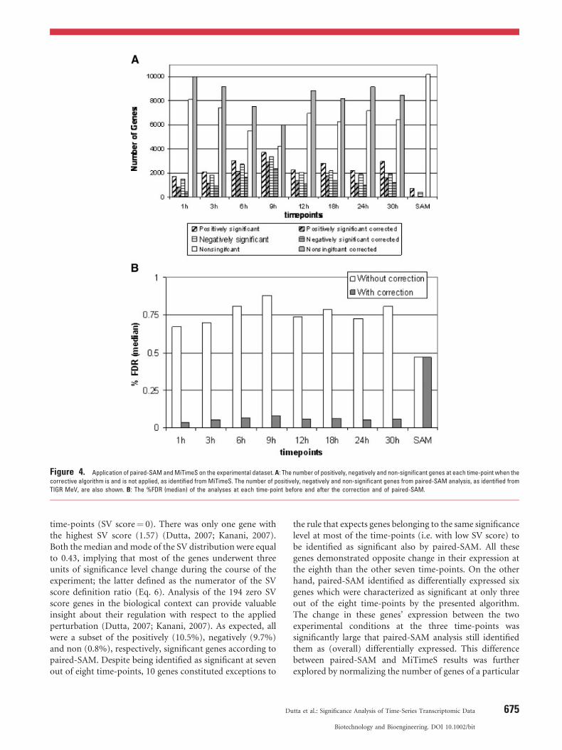
Figure 4. Application of paired-SAM andMiTimeS on the experimental dataset. A: The number of positively, negatively and non-significant genes at each time-point when the

corrective algorithm is and is not applied, as identified from MiTimeS. The number of positively, negatively and non-significant genes from paired-SAM analysis, as identified from

TIGR MeV, are also shown. B: The %FDR (median) of the analyses at each time-point before and after the correction and of paired-SAM.

time-points (SV score¼ 0). There was only one gene withthe highest SV score (1.57) (Dutta, 2007; Kanani, 2007).Both the median andmode of the SV distribution were equalto 0.43, implying that most of the genes underwent threeunits of significance level change during the course of theexperiment; the latter defined as the numerator of the SVscore definition ratio (Eq. 6). Analysis of the 194 zero SVscore genes in the biological context can provide valuableinsight about their regulation with respect to the appliedperturbation (Dutta, 2007; Kanani, 2007). As expected, allwere a subset of the positively (10.5%), negatively (9.7%)and non (0.8%), respectively, significant genes according topaired-SAM. Despite being identified as significant at sevenout of eight time-points, 10 genes constituted exceptions to

Du

the rule that expects genes belonging to the same significancelevel at most of the time-points (i.e. with low SV score) tobe identified as significant also by paired-SAM. All thesegenes demonstrated opposite change in their expression atthe eighth than the other seven time-points. On the otherhand, paired-SAM identified as differentially expressed sixgenes which were characterized as significant at only threeout of the eight time-points by the presented algorithm.The change in these genes’ expression between the twoexperimental conditions at the three time-points wassignificantly large that paired-SAM analysis still identifiedthem as (overall) differentially expressed. This differencebetween paired-SAM and MiTimeS results was furtherexplored by normalizing the number of genes of a particular



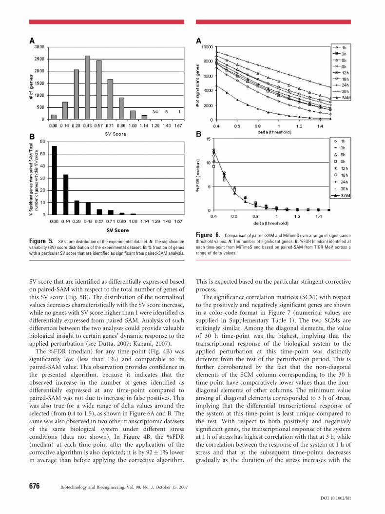
Figure 5. SV score distribution of the experimental dataset. A: The significance

variability (SV) score distribution of the experimental dataset. B: % fraction of genes

with a particular SV score that are identified as significant from paired-SAM analysis.

Figure 6. Comparison of paired-SAM and MiTimeS over a range of significance

threshold values. A: The number of significant genes. B: %FDR (median) identified at

each time-point from MiTimeS and based on paired-SAM from TIGR MeV across a

range of delta values.

SV score that are identified as differentially expressed basedon paired-SAM with respect to the total number of genes ofthis SV score (Fig. 5B). The distribution of the normalizedvalues decreases characteristically with the SV score increase,while no genes with SV score higher than 1 were identified asdifferentially expressed from paired-SAM. Analysis of suchdifferences between the two analyses could provide valuablebiological insight to certain genes’ dynamic response to theapplied perturbation (see Dutta, 2007; Kanani, 2007).

The %FDR (median) for any time-point (Fig. 4B) wassignificantly low (less than 1%) and comparable to itspaired-SAM value. This observation provides confidence inthe presented algorithm, because it indicates that theobserved increase in the number of genes identified asdifferentially expressed at any time-point compared topaired-SAM was not due to increase in false positives. Thiswas also true for a wide range of delta values around theselected (from 0.4 to 1.5), as shown in Figure 6A and B. Thesame was also observed in two other transcriptomic datasetsof the same biological system under different stressconditions (data not shown). In Figure 4B, the %FDR(median) at each time-point after the application of thecorrective algorithm is also depicted; it is by 92� 1% lowerin average than before applying the corrective algorithm.


This is expected based on the particular stringent correctiveprocess.

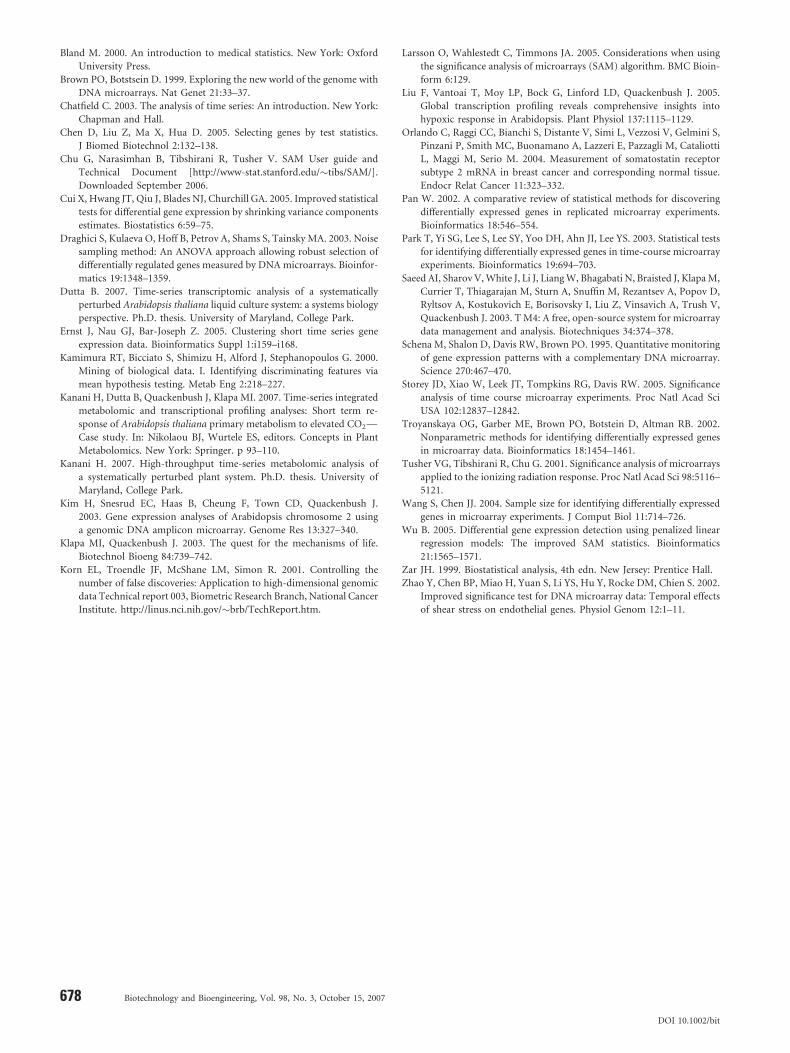
The significance correlation matrices (SCM) with respectto the positively and negatively significant genes are shownin a color-code format in Figure 7 (numerical values aresupplied in Supplementary Table 1). The two SCMs arestrikingly similar. Among the diagonal elements, the valueof 30 h time-point was the highest, implying that thetranscriptional response of the biological system to theapplied perturbation at this time-point was distinctlydifferent from the rest of the perturbation period. This isfurther corroborated by the fact that the non-diagonalelements of the SCM column corresponding to the 30 htime-point have comparatively lower values than the non-diagonal elements of other columns. The minimum valueamong all diagonal elements corresponded to 3 h of stress,implying that the differential transcriptional response ofthe system at this time-point is least unique compared tothe rest. With respect to both positively and negativelysignificant genes, the transcriptional response of the systemat 1 h of stress has highest correlation with that at 3 h, whilethe correlation between the response of the system at 1 h ofstress and that at the subsequent time-points decreasesgradually as the duration of the stress increases with the

DOI 10.1002/bit

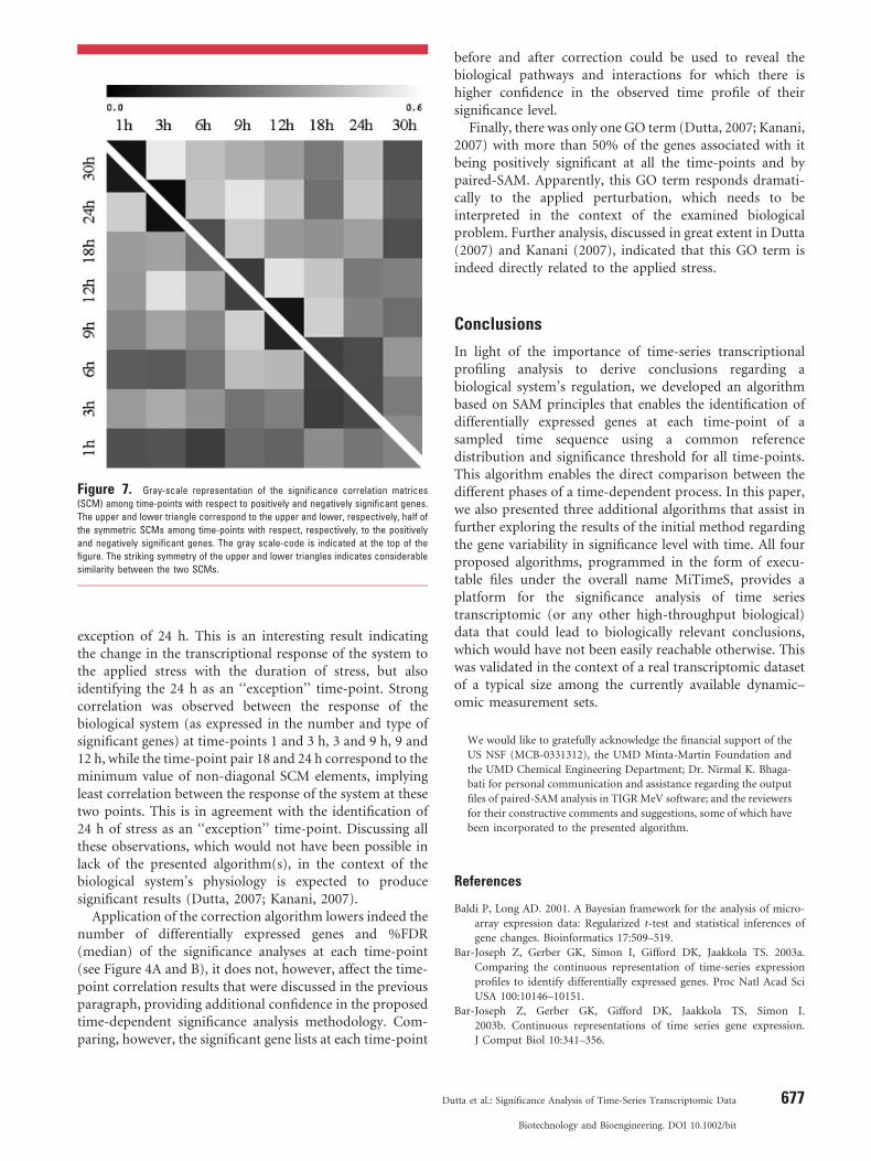
Figure 7. Gray-scale representation of the significance correlation matrices

(SCM) among time-points with respect to positively and negatively significant genes.

The upper and lower triangle correspond to the upper and lower, respectively, half of

the symmetric SCMs among time-points with respect, respectively, to the positively

and negatively significant genes. The gray scale-code is indicated at the top of the

figure. The striking symmetry of the upper and lower triangles indicates considerable

similarity between the two SCMs.

exception of 24 h. This is an interesting result indicatingthe change in the transcriptional response of the system tothe applied stress with the duration of stress, but alsoidentifying the 24 h as an ‘‘exception’’ time-point. Strongcorrelation was observed between the response of thebiological system (as expressed in the number and type ofsignificant genes) at time-points 1 and 3 h, 3 and 9 h, 9 and12 h, while the time-point pair 18 and 24 h correspond to theminimum value of non-diagonal SCM elements, implyingleast correlation between the response of the system at thesetwo points. This is in agreement with the identification of24 h of stress as an ‘‘exception’’ time-point. Discussing allthese observations, which would not have been possible inlack of the presented algorithm(s), in the context of thebiological system’s physiology is expected to producesignificant results (Dutta, 2007; Kanani, 2007).

Application of the correction algorithm lowers indeed thenumber of differentially expressed genes and %FDR(median) of the significance analyses at each time-point(see Figure 4A and B), it does not, however, affect the time-point correlation results that were discussed in the previousparagraph, providing additional confidence in the proposedtime-dependent significance analysis methodology. Com-paring, however, the significant gene lists at each time-point

Du

before and after correction could be used to reveal thebiological pathways and interactions for which there ishigher confidence in the observed time profile of theirsignificance level.

Finally, there was only one GO term (Dutta, 2007; Kanani,2007) with more than 50% of the genes associated with itbeing positively significant at all the time-points and bypaired-SAM. Apparently, this GO term responds dramati-cally to the applied perturbation, which needs to beinterpreted in the context of the examined biologicalproblem. Further analysis, discussed in great extent in Dutta(2007) and Kanani (2007), indicated that this GO term isindeed directly related to the applied stress.

Conclusions

In light of the importance of time-series transcriptionalprofiling analysis to derive conclusions regarding abiological system’s regulation, we developed an algorithmbased on SAM principles that enables the identification ofdifferentially expressed genes at each time-point of asampled time sequence using a common referencedistribution and significance threshold for all time-points.This algorithm enables the direct comparison between thedifferent phases of a time-dependent process. In this paper,we also presented three additional algorithms that assist infurther exploring the results of the initial method regardingthe gene variability in significance level with time. All fourproposed algorithms, programmed in the form of execu-table files under the overall name MiTimeS, provides aplatform for the significance analysis of time seriestranscriptomic (or any other high-throughput biological)data that could lead to biologically relevant conclusions,which would have not been easily reachable otherwise. Thiswas validated in the context of a real transcriptomic datasetof a typical size among the currently available dynamic–omic measurement sets.

We would like to gratefully acknowledge the financial support of the

US NSF (MCB-0331312), the UMD Minta-Martin Foundation and

the UMD Chemical Engineering Department; Dr. Nirmal K. Bhaga-

bati for personal communication and assistance regarding the output

files of paired-SAM analysis in TIGRMeV software; and the reviewers

for their constructive comments and suggestions, some of which have

been incorporated to the presented algorithm.

References

Baldi P, Long AD. 2001. A Bayesian framework for the analysis of micro-

array expression data: Regularized t-test and statistical inferences of

gene changes. Bioinformatics 17:509–519.

Bar-Joseph Z, Gerber GK, Simon I, Gifford DK, Jaakkola TS. 2003a.

Comparing the continuous representation of time-series expression

profiles to identify differentially expressed genes. Proc Natl Acad Sci

USA 100:10146–10151.

Bar-Joseph Z, Gerber GK, Gifford DK, Jaakkola TS, Simon I.

2003b. Continuous representations of time series gene expression.

J Comput Biol 10:341–356.



Bland M. 2000. An introduction to medical statistics. New York: Oxford

University Press.

Brown PO, Botstsein D. 1999. Exploring the new world of the genome with

DNA microarrays. Nat Genet 21:33–37.

Chatfield C. 2003. The analysis of time series: An introduction. New York:

Chapman and Hall.

Chen D, Liu Z, Ma X, Hua D. 2005. Selecting genes by test statistics.

J Biomed Biotechnol 2:132–138.

Chu G, Narasimhan B, Tibshirani R, Tusher V. SAM User guide and

Technical Document [http://www-stat.stanford.edu/�tibs/SAM/].

Downloaded September 2006.

Cui X, Hwang JT, Qiu J, Blades NJ, Churchill GA. 2005. Improved statistical

tests for differential gene expression by shrinking variance components

estimates. Biostatistics 6:59–75.

Draghici S, Kulaeva O, Hoff B, Petrov A, Shams S, Tainsky MA. 2003. Noise

sampling method: An ANOVA approach allowing robust selection of

differentially regulated genes measured by DNAmicroarrays. Bioinfor-

matics 19:1348–1359.

Dutta B. 2007. Time-series transcriptomic analysis of a systematically

perturbed Arabidopsis thaliana liquid culture system: a systems biology

perspective. Ph.D. thesis. University of Maryland, College Park.

Ernst J, Nau GJ, Bar-Joseph Z. 2005. Clustering short time series gene

expression data. Bioinformatics Suppl 1:i159–i168.

Kamimura RT, Bicciato S, Shimizu H, Alford J, Stephanopoulos G. 2000.

Mining of biological data. I. Identifying discriminating features via

mean hypothesis testing. Metab Eng 2:218–227.

Kanani H, Dutta B, Quackenbush J, Klapa MI. 2007. Time-series integrated

metabolomic and transcriptional profiling analyses: Short term re-

sponse of Arabidopsis thaliana primary metabolism to elevated CO2—

Case study. In: Nikolaou BJ, Wurtele ES, editors. Concepts in Plant

Metabolomics. New York: Springer. p 93–110.

Kanani H. 2007. High-throughput time-series metabolomic analysis of

a systematically perturbed plant system. Ph.D. thesis. University of

Maryland, College Park.

Kim H, Snesrud EC, Haas B, Cheung F, Town CD, Quackenbush J.

2003. Gene expression analyses of Arabidopsis chromosome 2 using

a genomic DNA amplicon microarray. Genome Res 13:327–340.

Klapa MI, Quackenbush J. 2003. The quest for the mechanisms of life.

Biotechnol Bioeng 84:739–742.

Korn EL, Troendle JF, McShane LM, Simon R. 2001. Controlling the

number of false discoveries: Application to high-dimensional genomic

data Technical report 003, Biometric Research Branch, National Cancer

Institute. http://linus.nci.nih.gov/�brb/TechReport.htm.


Larsson O, Wahlestedt C, Timmons JA. 2005. Considerations when using

the significance analysis of microarrays (SAM) algorithm. BMC Bioin-

form 6:129.

Liu F, Vantoai T, Moy LP, Bock G, Linford LD, Quackenbush J. 2005.

Global transcription profiling reveals comprehensive insights into

hypoxic response in Arabidopsis. Plant Physiol 137:1115–1129.

Orlando C, Raggi CC, Bianchi S, Distante V, Simi L, Vezzosi V, Gelmini S,

Pinzani P, Smith MC, Buonamano A, Lazzeri E, Pazzagli M, Cataliotti

L, Maggi M, Serio M. 2004. Measurement of somatostatin receptor

subtype 2 mRNA in breast cancer and corresponding normal tissue.

Endocr Relat Cancer 11:323–332.

Pan W. 2002. A comparative review of statistical methods for discovering

differentially expressed genes in replicated microarray experiments.

Bioinformatics 18:546–554.

Park T, Yi SG, Lee S, Lee SY, Yoo DH, Ahn JI, Lee YS. 2003. Statistical tests

for identifying differentially expressed genes in time-course microarray

experiments. Bioinformatics 19:694–703.

Saeed AI, Sharov V,White J, Li J, LiangW, Bhagabati N, Braisted J, KlapaM,

Currier T, Thiagarajan M, Sturn A, Snuffin M, Rezantsev A, Popov D,

Ryltsov A, Kostukovich E, Borisovsky I, Liu Z, Vinsavich A, Trush V,

Quackenbush J. 2003. T M4: A free, open-source system for microarray

data management and analysis. Biotechniques 34:374–378.

Schena M, Shalon D, Davis RW, Brown PO. 1995. Quantitative monitoring

of gene expression patterns with a complementary DNA microarray.

Science 270:467–470.

Storey JD, Xiao W, Leek JT, Tompkins RG, Davis RW. 2005. Significance

analysis of time course microarray experiments. Proc Natl Acad Sci

USA 102:12837–12842.

Troyanskaya OG, Garber ME, Brown PO, Botstein D, Altman RB. 2002.

Nonparametric methods for identifying differentially expressed genes

in microarray data. Bioinformatics 18:1454–1461.

Tusher VG, Tibshirani R, Chu G. 2001. Significance analysis of microarrays

applied to the ionizing radiation response. Proc Natl Acad Sci 98:5116–

5121.

Wang S, Chen JJ. 2004. Sample size for identifying differentially expressed

genes in microarray experiments. J Comput Biol 11:714–726.

Wu B. 2005. Differential gene expression detection using penalized linear

regression models: The improved SAM statistics. Bioinformatics

21:1565–1571.

Zar JH. 1999. Biostatistical analysis, 4th edn. New Jersey: Prentice Hall.

Zhao Y, Chen BP, Miao H, Yuan S, Li YS, Hu Y, Rocke DM, Chien S. 2002.

Improved significance test for DNA microarray data: Temporal effects

of shear stress on endothelial genes. Physiol Genom 12:1–11.

DOI 10.1002/bit

Significance analysis of time-series transcriptomic data: A methodology that enables the...

Documents

Transcript of Significance analysis of time-series transcriptomic data: A methodology that enables the...