Short note An improved geometry-aware curvature discretization for level set methods: Application to...
10
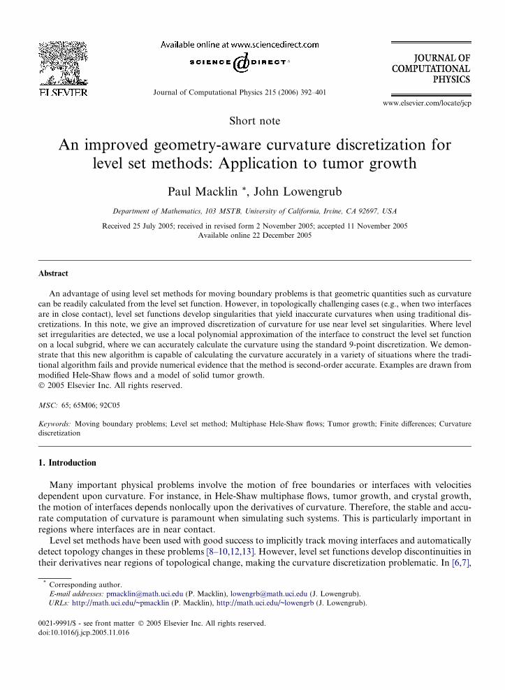
Short note An improved geometry-aware curvature discretization for level set methods: Application to tumor growth Paul Macklin * , John Lowengrub Department of Mathematics, 103 MSTB, University of California, Irvine, CA 92697, USA Received 25 July 2005; received in revised form 2 November 2005; accepted 11 November 2005 Available online 22 December 2005 Abstract An advantage of using level set methods for moving boundary problems is that geometric quantities such as curvature can be readily calculated from the level set function. However, in topologically challenging cases (e.g., when two interfaces are in close contact), level set functions develop singularities that yield inaccurate curvatures when using traditional dis- cretizations. In this note, we give an improved discretization of curvature for use near level set singularities. Where level set irregularities are detected, we use a local polynomial approximation of the interface to construct the level set function on a local subgrid, where we can accurately calculate the curvature using the standard 9-point discretization. We demon- strate that this new algorithm is capable of calculating the curvature accurately in a variety of situations where the tradi- tional algorithm fails and provide numerical evidence that the method is second-order accurate. Examples are drawn from modified Hele-Shaw flows and a model of solid tumor growth. Ó 2005 Elsevier Inc. All rights reserved. MSC: 65; 65M06; 92C05 Keywords: Moving boundary problems; Level set method; Multiphase Hele-Shaw flows; Tumor growth; Finite differences; Curvature discretization 1. Introduction Many important physical problems involve the motion of free boundaries or interfaces with velocities dependent upon curvature. For instance, in Hele-Shaw multiphase flows, tumor growth, and crystal growth, the motion of interfaces depends nonlocally upon the derivatives of curvature. Therefore, the stable and accu- rate computation of curvature is paramount when simulating such systems. This is particularly important in regions where interfaces are in near contact. Level set methods have been used with good success to implicitly track moving interfaces and automatically detect topology changes in these problems [8–10,12,13]. However, level set functions develop discontinuities in their derivatives near regions of topological change, making the curvature discretization problematic. In [6,7], 0021-9991/$ - see front matter Ó 2005 Elsevier Inc. All rights reserved. doi:10.1016/j.jcp.2005.11.016 * Corresponding author. E-mail addresses: [email protected] (P. Macklin), [email protected] (J. Lowengrub). URLs: http://math.uci.edu/~pmacklin (P. Macklin), http://math.uci.edu/~lowengrb (J. Lowengrub). Journal of Computational Physics 215 (2006) 392–401 www.elsevier.com/locate/jcp
Transcript of Short note An improved geometry-aware curvature discretization for level set methods: Application to...
Journal of Computational Physics 215 (2006) 392–401
www.elsevier.com/locate/jcp
Short note
An improved geometry-aware curvature discretization forlevel set methods: Application to tumor growth
Paul Macklin *, John Lowengrub
Department of Mathematics, 103 MSTB, University of California, Irvine, CA 92697, USA
Received 25 July 2005; received in revised form 2 November 2005; accepted 11 November 2005Available online 22 December 2005
Abstract
An advantage of using level set methods for moving boundary problems is that geometric quantities such as curvaturecan be readily calculated from the level set function. However, in topologically challenging cases (e.g., when two interfacesare in close contact), level set functions develop singularities that yield inaccurate curvatures when using traditional dis-cretizations. In this note, we give an improved discretization of curvature for use near level set singularities. Where levelset irregularities are detected, we use a local polynomial approximation of the interface to construct the level set functionon a local subgrid, where we can accurately calculate the curvature using the standard 9-point discretization. We demon-strate that this new algorithm is capable of calculating the curvature accurately in a variety of situations where the tradi-tional algorithm fails and provide numerical evidence that the method is second-order accurate. Examples are drawn frommodified Hele-Shaw flows and a model of solid tumor growth.� 2005 Elsevier Inc. All rights reserved.
MSC: 65; 65M06; 92C05
Keywords: Moving boundary problems; Level set method; Multiphase Hele-Shaw flows; Tumor growth; Finite differences; Curvaturediscretization
1. Introduction
Many important physical problems involve the motion of free boundaries or interfaces with velocitiesdependent upon curvature. For instance, in Hele-Shaw multiphase flows, tumor growth, and crystal growth,the motion of interfaces depends nonlocally upon the derivatives of curvature. Therefore, the stable and accu-rate computation of curvature is paramount when simulating such systems. This is particularly important inregions where interfaces are in near contact.
Level set methods have been used with good success to implicitly track moving interfaces and automaticallydetect topology changes in these problems [8–10,12,13]. However, level set functions develop discontinuities intheir derivatives near regions of topological change, making the curvature discretization problematic. In [6,7],
0021-9991/$ - see front matter � 2005 Elsevier Inc. All rights reserved.
doi:10.1016/j.jcp.2005.11.016
* Corresponding author.E-mail addresses: [email protected] (P. Macklin), [email protected] (J. Lowengrub).URLs: http://math.uci.edu/~pmacklin (P. Macklin), http://math.uci.edu/~lowengrb (J. Lowengrub).
P. Macklin, J. Lowengrub / Journal of Computational Physics 215 (2006) 392–401 393
it was demonstrated that if the curvature is computed without regard for the local geometry by using standardcentered difference algorithms as proposed in [8–10,12,13], then the curvature becomes oscillatory and inac-curate for interfaces in near contact. This may lead to sudden spikes in the curvature error. Refining the meshnear topology changes may delay the onset of these problems but cannot eliminate them. For example, weshow a case in which mesh refinement delays the formation of spikes but actually increases the spike magni-tude. In our example, this can lead to the blow-up of the solution when using a traditional curvature discret-ization. Furthermore, due to computational cost, mesh refinement cannot be continued indefinitely as thedistance between interfaces approaches zero.
In [6,7], a complicated curvature discretization was given that addressed the accurate approximation of cur-vature in complex 2D geometries in the context of a nonlinear model of tumor growth. In this paper, weintroduce a simpler and more robust geometry-aware curvature discretization that can be extended to 3dimensions. We calculate the curvature using standard level set methods when the level set function is suffi-ciently smooth. Otherwise, our method works by first constructing a properly-oriented (least squares, qua-dratic) polynomial approximation of the interface through a point. With this curve, we create a local levelset function with which to compute the curvature by a standard discretization on a local subgrid.
In our work, we have found that using a local level set function is more robust in calculating the curvaturethan directly differentiating an interpolating spline [6,7]. Alternative methods of representing the curve (e.g., B-splines; see [1,4,11]) can be used together with our method, but we find that quadratic least squares polynomialapproximations are easy to implement and sufficient for second-order accuracy.
Our method calculates the curvature accurately in a variety of difficult topological situations (e.g., merginginterfaces, drop fragmentation), as we demonstrate in examples of modified Hele-Shaw multiphase flow andin vivo tumor growth. In the Hele-Shaw example, we present numerical evidence of second-order convergence.Furthermore, we also demonstrate that in this example, the traditional curvature discretization fails in a waythat is worsened by decreasing the mesh size. Our method is generally applicable to any level set model involv-ing morphological changes or interfaces in near contact, e.g., multiphase flows (e.g., [13]), dendritic crystalgrowth (e.g., [3]), and image processing (e.g., [8,12]).
2. Overview
Traditional level set methods (e.g., [8–10,12,13]) compute curvature as
1 In
j ¼ r � rujruj
� �¼
uxxu2y � 2uxuyuxy þ uyyu
2x
ðu2x þ u2
yÞ3=2
; ð1Þ
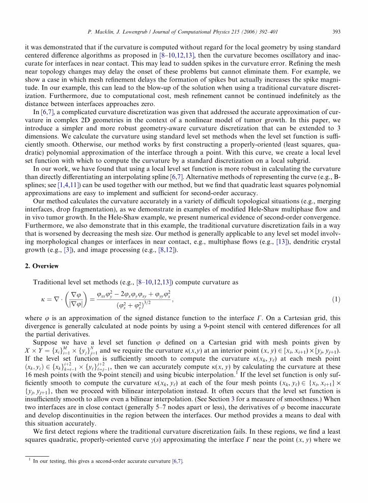
where u is an approximation of the signed distance function to the interface C. On a Cartesian grid, thisdivergence is generally calculated at node points by using a 9-point stencil with centered differences for allthe partial derivatives.
Suppose we have a level set function u defined on a Cartesian grid with mesh points given byX � Y ¼ fxigM
i¼1 � fyjgNj¼1 and we require the curvature j(x,y) at an interior point (x, y) 2 [xi, xi+1) · [yj, yj+1).
If the level set function is sufficiently smooth to compute the curvature j(xk, y‘) at each mesh pointðxk; y‘Þ 2 fxkgiþ2
k¼i�1 � fy‘gjþ2‘¼j�1, then we can accurately compute j(x, y) by calculating the curvature at these
16 mesh points (with the 9-point stencil) and using bicubic interpolation.1 If the level set function is only suf-ficiently smooth to compute the curvature j(xk, y‘) at each of the four mesh points (xk, y‘) 2 {xi, xi+1} ·{yj, yj+1}, then we proceed with bilinear interpolation instead. It often occurs that the level set function isinsufficiently smooth to allow even a bilinear interpolation. (See Section 3 for a measure of smoothness.) Whentwo interfaces are in close contact (generally 5–7 nodes apart or less), the derivatives of u become inaccurateand develop discontinuities in the region between the interfaces. Our method provides a means to deal withthis situation accurately.
We first detect regions where the traditional curvature discretization fails. In these regions, we find a leastsquares quadratic, properly-oriented curve c(s) approximating the interface C near the point (x, y) where we
our testing, this gives a second-order accurate curvature [6,7].
394 P. Macklin, J. Lowengrub / Journal of Computational Physics 215 (2006) 392–401
desire the curvature. We have found that directly differentiating c to obtain the curvature is not robust, as c issensitive to errors in the parameterization. Instead, we construct a local level set function bu about (x, y) anduse the standard 9-point stencil on a locally refined subgrid to discretize the curvature.
3. Detecting regions where the traditional curvature fails
In [6,7], we found that if we defined a level set quality function by
Qðx; yÞ ¼ j1� jrujj ð2Þ
and set a threshold g, then (x, y) is near a singularity of the level set function u whenever Q(x, y) P g; we com-pute $u using centered finite differences. In our testing, we found that using g = 0.004 reliably identified suchregions without yielding false positives.Suppose we wish to calculate the curvature at (xi, yj) using the standard 9-point discretization. If Q(x, y) Pg at any ðx; yÞ 2 fxkgiþ1
k¼i�1 � fx‘gjþ1‘¼j�1, then the level set function is not smooth enough to accurately discretize
the curvature at (xi, yj), and we use our geometry-aware algorithm instead.
4. Approximating the interface with proper orientation
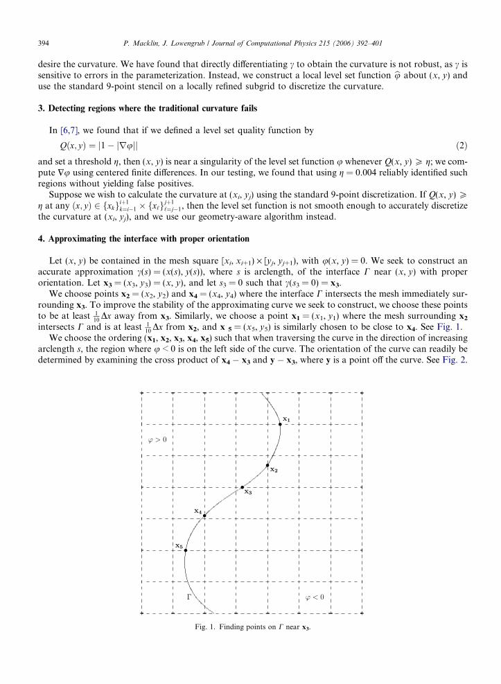
Let (x, y) be contained in the mesh square [xi, xi+1) · [yj, yj+1), with u(x, y) = 0. We seek to construct anaccurate approximation c(s) = (x(s), y(s)), where s is arclength, of the interface C near (x, y) with properorientation. Let x3 = (x3, y3) = (x, y), and let s3 = 0 such that c(s3 = 0) = x3.
We choose points x2 = (x2, y2) and x4 = (x4, y4) where the interface C intersects the mesh immediately sur-rounding x3. To improve the stability of the approximating curve we seek to construct, we choose these pointsto be at least 1
10Dx away from x3. Similarly, we choose a point x1 = (x1, y1) where the mesh surrounding x2
intersects C and is at least 110
Dx from x2, and x 5 = (x5, y5) is similarly chosen to be close to x4. See Fig. 1.We choose the ordering (x1, x2, x3, x4, x5) such that when traversing the curve in the direction of increasing
arclength s, the region where u < 0 is on the left side of the curve. The orientation of the curve can readily bedetermined by examining the cross product of x4 � x3 and y � x3, where y is a point off the curve. See Fig. 2.
Fig. 1. Finding points on C near x3.
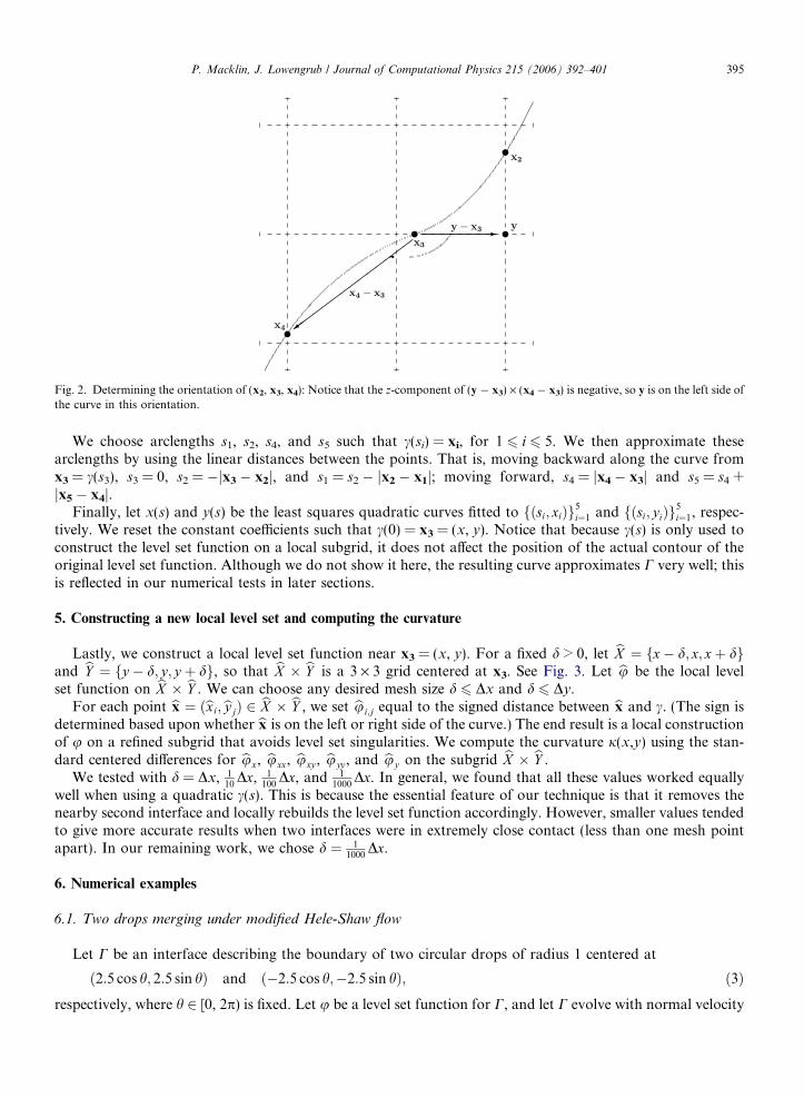
Fig. 2. Determining the orientation of (x2, x3, x4): Notice that the z-component of (y � x3) · (x4 � x3) is negative, so y is on the left side ofthe curve in this orientation.
P. Macklin, J. Lowengrub / Journal of Computational Physics 215 (2006) 392–401 395
We choose arclengths s1, s2, s4, and s5 such that c(si) = xi, for 1 6 i 6 5. We then approximate thesearclengths by using the linear distances between the points. That is, moving backward along the curve fromx3 = c(s3), s3 = 0, s2 = �jx3 � x2j, and s1 = s2 � jx2 � x1j; moving forward, s4 = jx4 � x3j and s5 = s4 +jx5 � x4j.
Finally, let x(s) and y(s) be the least squares quadratic curves fitted to fðsi; xiÞg5i¼1 and fðsi; yiÞg
5i¼1, respec-
tively. We reset the constant coefficients such that c(0) = x3 = (x, y). Notice that because c(s) is only used toconstruct the level set function on a local subgrid, it does not affect the position of the actual contour of theoriginal level set function. Although we do not show it here, the resulting curve approximates C very well; thisis reflected in our numerical tests in later sections.
5. Constructing a new local level set and computing the curvature
Lastly, we construct a local level set function near x3 = (x, y). For a fixed d > 0, let bX ¼ fx� d; x; xþ dgand bY ¼ fy � d; y; y þ dg, so that bX � bY is a 3 · 3 grid centered at x3. See Fig. 3. Let bu be the local levelset function on bX � bY . We can choose any desired mesh size d 6 Dx and d 6 Dy.
For each point bx ¼ ðbxi; by jÞ 2 bX � bY , we set bui;j equal to the signed distance between bx and c. (The sign isdetermined based upon whether bx is on the left or right side of the curve.) The end result is a local constructionof u on a refined subgrid that avoids level set singularities. We compute the curvature j(x,y) using the stan-dard centered differences for bux, buxx, buxy , buyy , and buy on the subgrid bX � bY .
We tested with d = Dx, 110
Dx, 1100
Dx, and 11000
Dx. In general, we found that all these values worked equallywell when using a quadratic c(s). This is because the essential feature of our technique is that it removes thenearby second interface and locally rebuilds the level set function accordingly. However, smaller values tendedto give more accurate results when two interfaces were in extremely close contact (less than one mesh pointapart). In our remaining work, we chose d ¼ 1
1000Dx.
6. Numerical examples
6.1. Two drops merging under modified Hele-Shaw flow
Let C be an interface describing the boundary of two circular drops of radius 1 centered at
ð2:5 cos h; 2:5 sin hÞ and ð�2:5 cos h;�2:5 sin hÞ; ð3Þ
respectively, where h 2 [0, 2p) is fixed. Let u be a level set function for C, and let C evolve with normal velocity
Fig. 3. The local subgrid near x3, with d ¼ 18Dx. In our tests, we used d ¼ 1
1000Dx.
396 P. Macklin, J. Lowengrub / Journal of Computational Physics 215 (2006) 392–401
V ¼ 1� n � ½rp� if uðxÞ ¼ 0; ð4Þ
where [$p] is the jump in the pressure gradient from the inside to the outside of the drops. The pressure psolves
r2p ¼ 0 if uðxÞ < 0; ð5Þ½p� ¼ j if uðxÞ ¼ 0; ð6Þp ¼ 0 if uðxÞ > 0; ð7Þ
where (6) is the Laplace–Young boundary condition, and the surface tension (the coefficient of the curvature)is non-dimensionalized to 1. The level set function u is updated via
ut þ V extjruj ¼ 0; ð8Þ
where Vext is an extension of V off of C.Under these equations, both circles expand outward at a constant speed of 1 since p � 11þt inside the drops
and p ” 0 outside the drops. At t = 1.5, the drops merge and thus become non-circular. Consequently, at thistime the curvature is no longer constant along the interface and instead takes large values near the intersec-tion. The pressure p inside the drops is then no longer constant, steep pressure gradients emerge, and the Hele-Shaw-like term of the velocity dominates near the intersection of the circles.
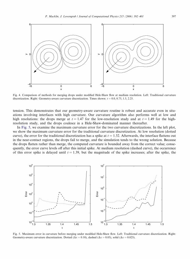
To study the convergence behavior of our curvature technique, we solved this example with h = 13� ona computational domain of [�6, 6] · [�6, 6] with Dx = Dy = 0.10 (low resolution), Dx = Dy = 0.05 (med-ium resolution), and Dx = Dy = 0.025 (high resolution) using the level set/ghost fluid method as describedin [7]. In Fig. 4, we show the medium-resolution results (Dx = 0.05), where the interfaces are plotted every0.75 time units from t = 0 to t = 2.25, and the arrows indicate the direction of growth. In the left plot, weshow the results when using the traditional 9-point curvature discretization. The singular curvaturebetween the merging interfaces creates steep and noisy false pressure gradients that prevent the mergerof the drops. This behavior of the traditional algorithm is also seen in the low-resolution study(Dx = 0.10), and at high resolution (Dx = 0.025), the traditional curvature algorithm becomes so inaccu-rate that the simulation is unable to continue past t = 1.486. This is a non-trivial example where the tra-ditional curvature discretization was inaccurate and led to incorrect simulation behavior, and decreasingDx exacerbated the problem.
On the right side of Fig. 4, we show the same simulation using our geometry-aware curvature discret-ization at medium resolution. (The high-resolution results are indistinguishable to graphical resolution.)Level set singularities between the merging interfaces are first detected at t = 1.33, and the discretizationadapts accordingly. The drops merge at approximately t = 1.48, very close to the exact time of t = 1.50.Immediately after the merger, sharp cusps form in the interface that are smoothed out due to surface
0 6
0
6
x
y
6 0 66
0
6
x
yFig. 4. Comparison of methods for merging drops under modified Hele-Shaw flow at medium resolution. Left: Traditional curvaturediscretization. Right: Geometry-aware curvature discretization. Times shown: t = 0.0, 0.75, 1.5, 2.25.
P. Macklin, J. Lowengrub / Journal of Computational Physics 215 (2006) 392–401 397
tension. This demonstrates that our geometry-aware curvature routine is robust and accurate even in situ-ations involving interfaces with high curvature. Our curvature algorithm also performs well at low andhigh resolutions: the drops merge at t = 1.47 for the low-resolution study and at t = 1.49 for the high-resolution study, and the drops coalesce in a Hele-Shaw-dominated manner thereafter.
In Fig. 5, we examine the maximum curvature error for the two curvature discretizations. In the left plot,we show the maximum curvature error for the traditional curvature discretization. At low resolution (dottedcurve), the error for the traditional discretization has a spike at t = 1.32. Afterwards, the interface flattens outin the near-contact regions, the drops fail to merge, and the simulation tends to the wrong solution. Becausethe drops flatten rather than merge, the computed curvature is bounded away from the correct value; conse-quently, the error curve levels off after this initial spike. At medium resolution (dashed curve), the occurrenceof this error spike is delayed until t = 1.39, but the magnitude of the spike increases; after the spike, the
1.3 1.35 1.4 1.45 1.510
102
100
102
104
106
108
t
Err
or
1.3 1.35 1.4 1.45 1.510
3
102
101
100
101
102
t
Err
or
Fig. 5. Maximum error in curvature before merging under modified Hele-Shaw flow. Left: Traditional curvature discretization. Right:Geometry-aware curvature discretization. Dotted (Dx = 0.10), dashed (Dx = 0.05), solid (Dx = 0.025).
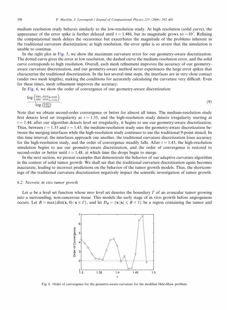
398 P. Macklin, J. Lowengrub / Journal of Computational Physics 215 (2006) 392–401
medium resolution study behaves similarly to the low-resolution study. At high resolution (solid curve), theappearance of the error spike is further delayed until t = 1.486, but its magnitude grows to �107. Refiningthe computational mesh delays the occurrence but exacerbates the magnitude of the problems inherent inthe traditional curvature discretization; at high resolution, the error spike is so severe that the simulation isunable to continue.
In the right plot in Fig. 5, we show the maximum curvature error for our geometry-aware discretization.The dotted curve gives the error at low resolution, the dashed curve the medium-resolution error, and the solidcurve corresponds to high resolution. Overall, each mesh refinement improves the accuracy of our geometry-aware curvature discretization, and our geometry-aware method never experiences the large error spikes thatcharacterize the traditional discretization. In the last several time steps, the interfaces are in very close contact(under two mesh lengths), making the conditions for accurately calculating the curvature very difficult. Evenfor these times, mesh refinement improves the accuracy.
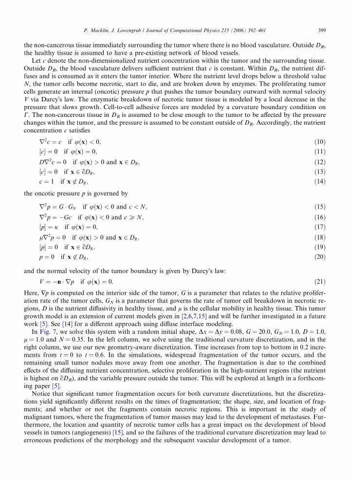
In Fig. 6, we show the order of convergence of our geometry-aware discretization:
log max errorDx¼0:025
max errorDx¼0:050
� �log 0:025
0:050
� � . ð9Þ
Note that we obtain second-order convergence or better for almost all times. The medium-resolution studyfirst detects level set irregularity at t = 1.33, and the high-resolution study detects irregularity starting att = 1.44; after our algorithm detects level set irregularity, it begins to use our geometry-aware discretization.Thus, between t = 1.33 and t = 1.43, the medium-resolution study uses the geometry-aware discretization be-tween the merging interfaces while the high-resolution study continues to use the traditional 9-point stencil. Inthis time interval, the interfaces approach one another, the traditional curvature discretization loses accuracyfor the high-resolution study, and the order of convergence steadily falls. After t = 1.43, the high-resolutionsimulation begins to use our geometry-aware discretization, and the order of convergence is restored tosecond-order or better until t = 1.48, at which time the drops begin to merge.
In the next section, we present examples that demonstrate the behavior of our adaptive curvature algorithmin the context of solid tumor growth. We shall see that the traditional curvature discretization again becomesinaccurate, leading to incorrect predictions on the behavior of the tumor growth models. Thus, the shortcom-ings of the traditional curvature discretization negatively impact the scientific investigation of tumor growth.
6.2. Necrotic in vivo tumor growth
Let u be a level set function whose zero level set denotes the boundary C of an avascular tumor growinginto a surrounding, non-cancerous tissue. This models the early stage of in vivo growth before angiogenesisoccurs. Let R = max{dist(x, 0) : x 2 C}, and let DR = {x:jxj 6 R + 1} be a region containing the tumor and
1.3 1.35 1.4 1.45 1.51
2
3
4
5
6
7
t
ecnegrevnoC fo redr
O
Fig. 6. Order of convergence for the geometry-aware curvature for the modified Hele-Shaw problem.
P. Macklin, J. Lowengrub / Journal of Computational Physics 215 (2006) 392–401 399
the non-cancerous tissue immediately surrounding the tumor where there is no blood vasculature. Outside DR,the healthy tissue is assumed to have a pre-existing network of blood vessels.
Let c denote the non-dimensionalized nutrient concentration within the tumor and the surrounding tissue.Outside DR, the blood vasculature delivers sufficient nutrient that c is constant. Within DR, the nutrient dif-fuses and is consumed as it enters the tumor interior. Where the nutrient level drops below a threshold valueN, the tumor cells become necrotic, start to die, and are broken down by enzymes. The proliferating tumorcells generate an internal (oncotic) pressure p that pushes the tumor boundary outward with normal velocityV via Darcy�s law. The enzymatic breakdown of necrotic tumor tissue is modeled by a local decrease in thepressure that slows growth. Cell-to-cell adhesive forces are modeled by a curvature boundary condition onC. The non-cancerous tissue in DR is assumed to be close enough to the tumor to be affected by the pressurechanges within the tumor, and the pressure is assumed to be constant outside of DR. Accordingly, the nutrientconcentration c satisfies
r2c ¼ c if uðxÞ < 0; ð10Þ½c� ¼ 0 if uðxÞ ¼ 0; ð11ÞDr2c ¼ 0 if uðxÞ > 0 and x 2 DR; ð12Þ½c� ¼ 0 if x 2 oDR; ð13Þc ¼ 1 if x 62 DR; ð14Þ
the oncotic pressure p is governed by
r2p ¼ G � GN if uðxÞ < 0 and c < N ; ð15Þr2p ¼ �Gc if uðxÞ < 0 and c P N ; ð16Þ½p� ¼ j if uðxÞ ¼ 0; ð17Þlr2p ¼ 0 if uðxÞ > 0 and x 2 DR; ð18Þ½p� ¼ 0 if x 2 oDR; ð19Þp ¼ 0 if x 62 DR; ð20Þ
and the normal velocity of the tumor boundary is given by Darcy�s law:
V ¼ �n � rp if uðxÞ ¼ 0. ð21Þ
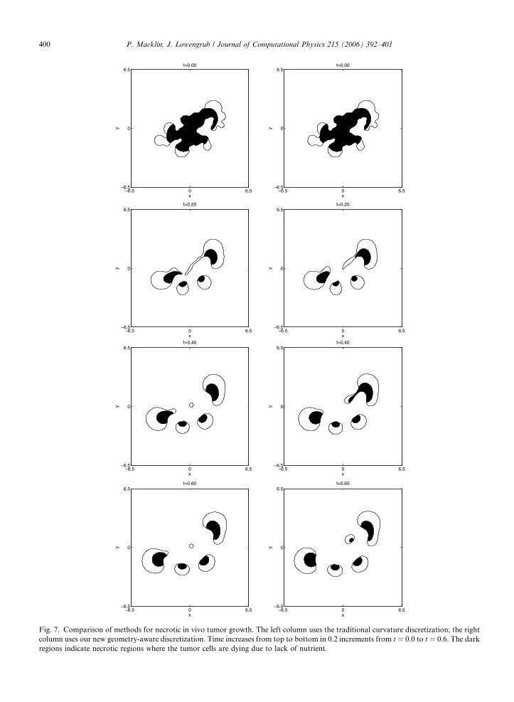
Here, $p is computed on the interior side of the tumor, G is a parameter that relates to the relative prolifer-ation rate of the tumor cells, GN is a parameter that governs the rate of tumor cell breakdown in necrotic re-gions, D is the nutrient diffusivity in healthy tissue, and l is the cellular mobility in healthy tissue. This tumorgrowth model is an extension of current models given in [2,6,7,15] and will be further investigated in a futurework [5]. See [14] for a different approach using diffuse interface modeling.In Fig. 7, we solve this system with a random initial shape, Dx = Dy = 0.08, G = 20.0, GN = 1.0, D = 1.0,l = 1.0 and N = 0.35. In the left column, we solve using the traditional curvature discretization, and in theright column, we use our new geometry-aware discretization. Time increases from top to bottom in 0.2 incre-ments from t = 0 to t = 0.6. In the simulations, widespread fragmentation of the tumor occurs, and theremaining small tumor nodules move away from one another. The fragmentation is due to the combinedeffects of the diffusing nutrient concentration, selective proliferation in the high-nutrient regions (the nutrientis highest on oDR), and the variable pressure outside the tumor. This will be explored at length in a forthcom-ing paper [5].
Notice that significant tumor fragmentation occurs for both curvature discretizations, but the discretiza-tions yield significantly different results on the times of fragmentation; the shape, size, and location of frag-ments; and whether or not the fragments contain necrotic regions. This is important in the study ofmalignant tumors, where the fragmentation of tumor masses may lead to the development of metastases. Fur-thermore, the location and quantity of necrotic tumor cells has a great impact on the development of bloodvessels in tumors (angiogenesis) [15], and so the failures of the traditional curvature discretization may lead toerroneous predictions of the morphology and the subsequent vascular development of a tumor.
5 0 6.55
0
6.5
x
y
t=0.00
6.5 0 6.56.5
0
6.5
x
y
t=0.00
6.5 0 6.56.5
0
6.5
x
y
t=0.20
6.5 0 6.56.5
0
6.5
x
y
t=0.20
6.5 0 6.56.5
0
6.5
x
y
t=0.40
6.5 0 6.56.5
0
6.5
x
y
t=0.40
6.5 0 6.56.5
0
6.5
x
y
t=0.60
6.5 0 6.56.5
0
6.5
x
y
t=0.60
Fig. 7. Comparison of methods for necrotic in vivo tumor growth. The left column uses the traditional curvature discretization; the rightcolumn uses our new geometry-aware discretization. Time increases from top to bottom in 0.2 increments from t = 0.0 to t = 0.6. The darkregions indicate necrotic regions where the tumor cells are dying due to lack of nutrient.
400 P. Macklin, J. Lowengrub / Journal of Computational Physics 215 (2006) 392–401
P. Macklin, J. Lowengrub / Journal of Computational Physics 215 (2006) 392–401 401
7. Conclusions
We have developed an improved geometry-aware discretization of curvature for use near level set singular-ities. In our method, we first detect regions where the traditional curvature discretization fails. Then, we find aleast squares, oriented quadratic polynomial approximation of the interface centered at the point where wedesire the curvature. A local level set function is constructed, and a standard 9-point stencil is used on a localsubgrid to discretize the curvature.
We have demonstrated that for complex geometries (e.g., interfaces in near contact), the traditional curva-ture discretization produced results that were not improved by mesh refinement, whereas our geometry-awarealgorithm was second-order accurate and robust. Examples were given for modified Hele-Shaw flow andin vitro tumor growth. In the tumor growth example, it was demonstrated that an accurate and robust cur-vature discretization is critical for the accurate modeling of the biophysical properties of evolving tumors.Our method is generally applicable to any level set model involving morphological changes or interfaces innear contact, e.g., multiphase flows, dendritic crystal growth, and image processing.
Lastly, we note that the geometry-aware curvature discretization developed here can be extended to threedimensions by finding an approximating surface c(s1, s2) = (x(s1, s2), y(s1, s2), z(s1, s2)) and constructing a3 · 3 · 3 local level set function. We also note that this method could be used to improve the accuracy ofnormal vector discretizations near level set singularities; this is currently under study.
Acknowledgements
The authors gratefully thank Vittorio Cristini and Steven Wise for enlightening discussions concerning thiswork. The authors also thank the Network and Academic Computing Services (NACS) at the University ofCalifornia at Irvine (UCI) and the departments of mathematics and biomedical engineering at UCI for gen-erous computing resources. We thank the National Science Foundation (mathematics division) for partialsupport.
References
[1] C. de Boor, A Practical Guide to Splines, Springer-Verlag, New York, 1978.[2] V. Cristini, J.S. Lowengrub, Q. Nie, Nonlinear simulation of tumor growth, J. Math. Biol. 46 (2003) 191–224.[3] F. Gibou, R. Fedkiw, R. Caflisch, S. Osher, A level set approach for the numerical simulation of dendritic growth, J. Sci. Comput. 19
(2003) 183–199.[4] W. Li, S. Xu, G. Zhao, L.P. Goh, Adaptive knot placement in B-spline curve approximation, Comput. Aided Des. 37 (8) (2005) 791–
797.[5] J.S. Lowengrub, P. Macklin, Nonlinear simulation of in vitro and in vivo tumor growth, in preparation.[6] P. Macklin, Numerical simulation of tumor growth and chemotherapy, M.S. Thesis, University of Minnesota School of Mathematics,
September 2003.[7] P. Macklin, J.S. Lowengrub, Evolving interfaces via gradients of geometry-dependent interior Poisson problems: Application to
tumor growth, J. Comput. Phys. 203 (1) (2005) 191–220.[8] S. Osher, R. Fedkiw, Level Set Methods and Dynamic Implicit Surfaces, Springer, New York, NY, 2002, ISBN 0-387-95482-1.[9] S. Osher, R. Fedkiw, Level set methods: an overview and some recent results, J. Comput. Phys. 169 (2) (2001) 463–502.
[10] S. Osher, J.A. Sethian, Fronts propagating with curvature-dependent speed: algorithms based on Hamilton–Jacobi formulations, J.Comput. Phys. 79 (1988) 12–49.
[11] A.E. Segall, M.J. Sipics, The influence of interpolation errors on finite-element calculations involving stress-curvature proportion-alities, Finite Elem. Anal. Des. 40 (13-14) (2004) 1873–1884.
[12] J.A. Sethian, Level Set Methods and Fast Marching Methods, Cambridge University Press, New York, NY, 1999, ISBN 0-521-64557-3.
[13] J.A. Sethian, P. Smereka, Level set methods for fluid interfaces, Ann. Rev. Fluid Mech. 35 (2003) 341–372.[14] S. Wise, H. Frieboes, V. Cristini, Three-dimensional simulation of the growth of a multispecies tumor via a diffuse interface approach,
Bull. Math. Biol., in review.[15] X. Zheng, S.M. Wise, V. Cristini, Nonlinear simulation of tumor necrosis, neo-vascularization and tissue invasion via an adaptive
finite-element/level set method, Bull. Math. Biol. 67 (2005) 211–259.