Shifting of Localization Planes in Optical Testing: Application to a Shearing Interferometer

Shifting of localization planes in optical testing:application to a shearing interferometer

Juan M. Simon, Silvia A. Comastri, and Rodolfo M. Echarri

An amplitude-division two-beam interferometer illuminated by a quasi-monochromatic, spatially inco-herent, and periodic source yields multiple localization planes of interference fringes. If a thick trans-mission sample with a few localized phase disturbances in various layers is placed in the interferometer,the disturbances in a layer can be detected, making its images through the two arms coincide with achosen localization plane. Different layers can be analyzed by means of shifting the localization planeby a variation of the source period without any other changes in the device. Here we illustrate thismethod by applying it to a shearing interferometer, a classical Wollaston prism placed between crossedpolarizers. Experimental images of different observation planes are obtained, and they are in goodagreement with the theoretical expectations. © 2001 Optical Society of America

OCIS codes: 120.0120, 120.3180.

1. Introduction

Optical testing is one of the classical applications ofinterferometry, and phase differences can be deter-mined with high accuracy1–3 by use of various meth-ods.4,5 To allow for interferometric measurements,an adequate contrast of fringes must be achieved.The dream of attaining high coherence at a timewhen the laser did not exist turned, in many cases,into a nightmare after its invention because of theassociated coherent noise. To obtain the desiredmutual coherence avoiding coherent noise, a classicalprocedure is to illuminate an amplitude-division in-terferometer with an extended incoherent quasi-monochromatic source so that localized fringesappear.6–8 This technique is particularly interest-ing, since, when the device is adjusted such that thetested surface �or its images through the interferom-eter� coincides with a localization plane, an ideal pre-sentation of the desired information is obtained,whereas small defects of the other optical elementscomposing the system are imperceptible. A method

to calculate disturbances distributed in a transparentsample is to record interferograms from a variety ofviewing directions and to process the informationwith computational algorithms.9

When the extended source is continuous, a two-beam amplitude-division interferometer yields a lo-calization plane, the classical one, and consequently,to test different layers of a transparent sample, thedevice must be readjusted to displace this plane.Nevertheless, there are certain sources and�or inter-ferometers that yield various localization planes in-stead of only one. A well-known example of theseinterferometers is the Ronchi grating,10 though inthis case there are multiple beam interferences �Laufringes�. In recent papers we have shown that anytwo-beam amplitude-division interferometer withplane symmetry illuminated by a periodic array ofquasi-monochromatic incoherent sources can yieldmultiple planes of interference.11–13 This configura-tion can be employed to detect disturbances presenton a layer of a transparent sample by means of map-ping them on a nonclassical localization plane, anddifferent layers can be tested by means of shifting thelocalization plane by a change of the source period.The periodic array of sources can be obtained, e.g.,when a Ronchi grating is placed in front of an inco-herent continuous source, and its period can be mod-ified either by steps, by changing the grating, or in acontinuous way, by use of zoom lenses. The methodwe propose avoids the need to readjust the inter-ferometer; however, to analyze the information prop-

The authors are with the Laboratorio de Optica, Facultad deCiencias Exactas y Naturales, Universidad de Buenos Aires,1428 Buenos Aires, Argentina. S. A. Comastri �[email protected]� and R. M. Echarri are also with the Consejo Nacional deInvestigaciones Cientificas y Tecnicas, Buenos Aires, Argentina.

Received 1 November 2000; revised manuscript received 8 May2001.

0003-6935�01�284999-12$15.00�0© 2001 Optical Society of America

1 October 2001 � Vol. 40, No. 28 � APPLIED OPTICS 4999

erly, it is limited to samples with just a few, relativelysmall and well-localized perturbations.

To illustrate the method, in a recent paper we ap-plied it to a Mach–Zehnder interferometer,14 and inthe present one we apply it to a shearing interferom-eter, a classical Wollaston prism between crossed po-larizers.13 The Wollaston is less versatile thoughmore easy to align than the Mach–Zehnder and hasthe drawback that a disturbance present in a trans-parent sample appears in both arms. In Section 2we give the notation and assumptions used and ex-plain our method. In Section 3 we show experimen-tal and theoretical results obtained when we placeinto the source space of a Wollaston prism a trans-mission sample consisting of a glass plate approxi-mately 10 mm thick coated on both faces with zincsulphide and with a scratch on each face. In Appen-dix A we give a brief review of the multilocalizationphenomenon �a complete analysis is given in our pre-vious paper12�. Finally, in Appendix B we define theinterferometer parameters following Steel,1 and werelate the shear at the exit and the entrance.

2. Optical Testing with a Shearing Interferometer

In a former paper12 we considered an amplitude-division interferometer with two arms, labeled I andII, illuminated by quasi-monochromatic radiation ofmean wavelength in vacuum �� . The source, �, wasspatially incoherent and periodic, of period �x and

size 2H; it lay on a plane �x, y� perpendicular to anaxis z, and the origin of system �x, y, z� was at thecentral source point, O. Assuming negligible equiv-alent aberrations and the validity of the constantcontrast condition, we derived expressions �which werewrite in Appendix A� for the intensity, I�P��, andthe degree of coherence, �I,II�P�� I,II�P��expi arg�I,II�P��, at a point P� of an observation plane ��.

In the present paper we consider that the inter-ferometer is of the shearing type and has lateralshear in any localization plane, except in the classicalone where it is assumed to be zero, and that prior tothe interferometer there is a sample consisting of aplane-parallel transparent plate with just a fewphase disturbances. The equations given in Appen-dix A also hold in this case if the source � is replacedwith an effective source, termed �, which is the imageof � through the sample. The central point of � istermed O, and the images of � �and O� through botharms are �� and �� and O� and O��.

A. Notation and Assumptions

Any ray from O incident on the interferometer splitsinto two rays that intersect at a point P�loc of theclassical localization plane, ��0. For simplicity weassume the device to be adjusted as in Fig. 1, and sowe have that �i� there is translational symmetryalong the y axis i.e., only plane �x, z� needs to beconsidered; �ii� the ray from O traveling along z gives

Fig. 1. Shearing interferometer �S.I.�: �, source; �x, y�, coordinates at the source plane; z, normal to the source; O, central source point;T, sample with a disturbance surrounding one point; �, image of � through the sample; O, effective central source point giving rise to awave front that has a disturbance around point Q when it immediately leaves T; O� or O� �and Q� or Q��, images of O �and Q� through armsI or II; x�, axis containing O� and O�; S�k and S�k, images of an arbitrary source point; P�loc,o, point of the classical localization plane ��0 suchthat O�P�loc,o � O�P�loc,o; “Io” and “IIo”, rays O�P�loc,o and O�P�loc,o; z�, axis perpendicular to x� and containing P�loc,o; P�o and P�, points on theobservation plane ��; �, axis parallel to x� with origin at P�o; B� �and B��, point where the ray “Io” �and “IIo”� intersects the � axis; D�,distance from plane � x�, y�� to � �, �� y� and �� not shown for simplicity�; s�o � B�B�, shear.

5000 APPLIED OPTICS � Vol. 40, No. 28 � 1 October 2001

rise to rays O�P�loc,o and O�P�loc,o �for short termed “Io”and “IIo”� such that O�P�loc,o � O�P�loc,o; �iii� the bifur-cation angle between rays “IIo” and “Io”, termed ��o,verifies the paraxial approximation; �iv�we define theaxis x� as that containing O� and O�, and perpendic-ular to it there is an axis, z�, that contains point P�loc,o;and �v� �� and �� have equal magnifications and lie onplanes that may be slightly inclined with respect tothe plane � x�, y�� y� being perpendicular to x� andparallel to y�. Under these conditions, at the exit wecan consider only one coordinate system, � x�, y�, z��;the lead is l�o � O� P�loc,o � O�P�loc,o � 0, and the tilt�defined as the lateral separation between the raysO�P�loc,o and O�P�loc,o� is t�o � O�O� �we define theseparameters following Steel,1 and we give a brief re-view in Appendix B�.

At a plane �� a distance D� apart from plane � x�, y��with �D�� t�o��, we define a coordinate system � �,��, parallel to � x�, y�� and with origin at a point P�o,which is on the y� axis. Rays “Io” and “IIo” intersectplane � �, �� at points B� and B�. If the distancefrom P�loc,o to P�o �or to B�� is K� �or Z�� and the distancefrom O� to P�loc,o is F�, then

K� � Z� cos��o�2� � Z�,

F� � O�P�loc,o �D� � K�

cos��o�2�� D� � K�. (1)

The images of P�o back through arms I and II aretermed PIo and PIIo, and, regarding the shift as neg-ligible, PIo and PIIo are in a plane a distance D apartfrom that containing �. The shear in the source andobservation representations are so � PIIoPIo and s�o �B�B�, respectively, and, according to Eq. �B1�, theyare related by n � H � so�D � n� � H� � s�o�D��2H and 2H� being the sizes of � and ��. Moreover,from Fig. 1 we obtain s�o � ��oK�, and hence s�o isproportional to K�.

B. Interferometer Exit

We analyze how the interferometer exit varies ac-cording to the source employed.

1. Linear SourceIf the source is linear, then in the plane � x�, z�� onlypoint O is present. For simplicity, first we regardthe sample as containing only one small disturbancesurrounding a point in its back surface. The wavefront emerging from O is distorted with respect to theideal spherical shape as it passes through the sample.When this wave front immediately leaves the sample,it exhibits a local disturbance in the neighborhood ofa point, which we denote Q, and as it propagates, itsshape varies. This wave front splits in the inter-ferometer, originating two wave fronts with nominalcurvature centers at O� and O�, and one is inclinedin ��o with respect to the other. The observationplane containing the images of Q through both arms,Q� and Q�, is termed ��M; here the interfering wavefronts have the same small localized error near Q�and Q�, and their disturbances map the one at the

sample �see Fig. 1�. At any exit point P� the inten-sity associated with point O �the one corresponding toan extended source is given in Eq. �A3� is

IO�P�� I�I��P�� I�II��P�� 2I�I��P��

� I�II��P��1�2 cos�O� �, ��. (2)

The phase difference in P�, �O� �, ��, can be writtenas

�O� �, �� O� � �2�� O�P� � O�P��, (3)

where � denotes optical path and ��O� is indepen-dent of P� and is defined as

��O� � �I,II � �2�� OO� � OO��, (4)

with �I,II � �I � �II ��I and �II take into account thephase shifts of the portion of the light travelingthrough arms I and II�. In the ideal case the inter-fering wave fronts are spherical, and if � �� D� and �0j

is the coordinate for the jth bright fringe � j inte-ger�, the fringe spacing Eqs. �1� and �A9� is

�D� � �0� j�1� � �0j��

n��D��t�o�

��

n��o��1 �

K�

F�� 0��1 �

K�

F�� , (5)

��0� being the fringe spacing at ��0, and, since 2j� ��O� � �2� �0j

��D�, the fringes are straight. In thereal case we define the deformation at point P� of thewave fronts that have vertices at B� and B�, which wedenote w�� , �� and w�� , ��, respectively, as theoptical path length from the ideal sphere to the realwave front. In this case,

�O� �, �� O� �2��D�

� � �2�� w�� , ��

� w�� , ��, (6)

and the fringes constitute isolines of equal phase dif-ference. The way in which the error present in thewave fronts causes the fringes to depart from straightlines depends on the relation between s�o and thedisturbance width along �, which we denote e�o �inFig. 1 we show the disturbance width e�M at ��M�. Ifthe disturbance width is less than the shear �i.e., if�e�o�s�o�� 1� and if � �j, ��j� are the coordinates for the jthbright fringe, then from Eq. �6�,

�j � �0j� ��D�� w�� j, ��j� � w�� j, ��j�, (7)

but, depending on which P� is considered, w�� , �� orw�� , �� or both can be zero, so the fringes are levellines indicating the amount of perturbation presentin the wave fronts, and, for each localized error in thesample, the fringe pattern is distorted twice. How-ever, when the disturbance width is greater than theshear, the regions with disturbances on both wavefronts are superposed, and, since w�� , �� w��


s�o, �� see Fig. 1�, if �e�o�s�o�� 1, Eq. �7� can be writtenas

�j � �0j�

�D�

��s�o�w��

�� ,��

, (8)

so the fringe pattern is distorted once. Conse-quently, when the observation plane contains the im-ages through both arms of the disturbance in thewave front immediately leaving the sample, we canevaluate either the deformation of the wave frontsw�� , �� or w�� , �� in Eq. �7� or the derivative�w�� j,�� in Eq. �8�, using an adequate phaseevaluation method,5 and these data can be related tothe perturbations present in the sample. However,this calculation is not our aim in the present publi-cation.

Moreover, when the sample contains disturbancesdistributed in different layers, because of the largelocalization and focalization depths, the fringes at ��Mappear superposed to fringes corresponding to otherlayers.

2. Extended, Incoherent, Continuous SourceIn this case the fringes are seen only at ��0, where weassume that there is no shear, so the fringes arestraight, and the disturbance present in the samplecannot be detected.

3. Extended, Incoherent, Periodic SourceWhen the source is spatially incoherent and periodic,the inconveniences appearing in the preceding casesare overcome, since there are localization planes ofdifferent orders m �with m integer�, which we denote��m. According to Eqs. �A5�–�A7�, since K� � Z� Eq.�1�, the degree of coherence is

�I,II�P��0 �1N

sin ��

sin��N�sin��

,

� �ba10�P��

2, � �

�xa10�P��2

,

a10�P�� 2�q1

��0�

K�

�F� � K��, (9)

and from Eq. �A8� the localization planes ��m are ex-pected to be located at a distance K�m from ��0 given by

K�m �F�m��0�

q1�x � m��0� , q1 �H�

H. (10)

When the sample contains only one small distur-bance surrounding a point in its back surface, if alocalization plane coincides with ��M, then the inter-ferogram maps this disturbance or its derivative, notonly considering point O but also any other sourcepoint Sk. This is because, although a perturbatedwave front changes its shape as it propagates, at ��Mthe wave fronts originated at O� and S�k �and at O�and S�k� are distorted approximately in the same re-gion and in a similar way �see Fig. 1�. To calculate

the phase at a point P�M of ��M, the term arg�I,II�P�M�has to be considered Eq. �A4�, but, since the deviceis assumed to verify the constant contrast condi-tion,12 this term is locally independent of P�M. Thuswe define

�� arg�I,II�P�� I,II � �2�� OO� � OO��,

(11)

and Eqs. �3�–�8� hold, when in Eq. �3� ��O� is replacedwith �� and �O� �, �� is replaced with the phasedifference �� , ��. On the localization planes near��M, the fringes are distorted, though their shapeslightly differs from that at ��M; they are a little de-focused because the localization depth is differentfrom zero and because the disturbance at the samplecan be distributed in a volume surrounding the con-sidered point. Contrarily, when the localizationplane is sufficiently far from ��M, fringes are expectedto be seen on other localization planes, but, in thiscase, the wave front associated with each source pointhas a different deformation and therefore originates adifferent distortion of fringes, so each source pointyields a different interferogram, and the superposi-tion of these results in a pattern of low-contrast andalmost straight fringes.

Furthermore, if the sample contains various dis-turbances surrounding points distributed in differentlayers, we can detect the deformations in each layerby leaving the sample in a fixed position and shiftingthe localization plane to the plane that contains thetwo images of the considered layer by means of avariation of the source period. That is, from Eq.�10�, if F� and ��0� are fixed �i.e., if the interferometeris neither displaced nor readjusted�, the localizationplanes with m� 0 can be shifted by means of varying�x. In the particular case in which m � 0, plane ��mis to the left of plane ��0 and moves toward ��0 when �xincreases.

3. Experimental Configuration and Results

We describe the experimental configuration used andshow the images acquired in different observationplanes, comparing them with the theoretical expec-tations.

A. Experimental Configuration

The device consists of an illumination system, a Wol-laston prism, and an observation system, and it isadjusted such that the axes z and z� coincide and arealong the optical bench. The source plane, the clas-sical localization plane, and the plane containingboth images of the source through the interferometerare perpendicular to z �Fig. 2�.

1. Illumination Optical SystemThe illumination optical system consists of an inco-herent source and a transmission sample. Thesource is composed of a mercury source, a condenser,and a mask that can be either a thin slit or a grating.We use a set of eight gratings �slits parallel to the y


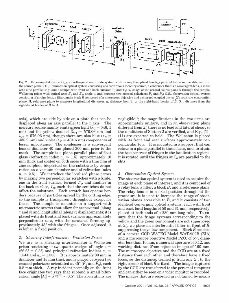
axis�, which are side by side on a plate that can bedisplaced along an axis parallel to the x axis. Themercury source mainly emits green light ��G� 546, 1nm� and the yellow doublet ��y1 � 579.06 nm and��y2 � 576.96 nm�, though there are also blue ��B �435.9 nm� and violet ��V � 404.6 nm� components oflesser importance. The condenser is a convergentlens of diameter 40 mm placed 300 mm prior to themask. The sample is a plane-parallel plate of floatglass �refraction index ng � 1.5�, approximately 10mm thick and coated on both sides with a thin film ofzinc sulphide �deposited on the substrate by evapo-ration on a vacuum chamber and of refraction indexnz � 2.5�. We introduce the localized phase errorsby making two perpendicular scratches with a knife,one in the front surface, termed T1, and another inthe back surface, T2, such that the scratches do notaffect the substrate. Each scratch has opaque bor-ders because of particles spread by the cutting edge,so the sample is transparent throughout except forthese. The sample is mounted in a support withmicrometric screws that allow for transversal �alongx and y� and longitudinal �along z� displacements; it isplaced with its front and back surfaces approximatelyperpendicular to z, with the scratches forming ap-proximately 45° with the fringes. Once adjusted, itis left in a fixed position.

2. Shearing Interferometer: Wollaston PrismWe use as a shearing interferometer a Wollastonprism consisting of two quartz wedges of angle � ��26.6° � 0.3°� and principal refraction indices no �1.544 and ne � 1.553. It is approximately 30 mm indiameter and 15 mm thick and is placed between twocrossed polarizers orientated at 45° �P1 and P2�, each0.8 mm thick. A ray incident normally on the frontface originates two rays that subtend a small bifur-cation angle ��o� � ��0� � 0.5°. The aberrations are

negligible13; the magnifications in the two arms areapproximately unitary, and in an observation planedifferent from ��0 there is no lead and lateral shear, sothe conditions of Section 2 are verified, and Eqs. �1�–�11� are expected to hold. The Wollaston is placedwith its front and rear surfaces approximately per-pendicular to z. It is mounted in a support that canrotate in a plane parallel to these faces, and, to attainthe best contrast of fringes in the localization regions,it is rotated until the fringes at ��0 are parallel to theslits.

3. Observation Optical SystemThe observation optical system is used to acquire theimage at each plane of interest, and it is composed ofa relay lens, a filter, a block B, and a reference plane.The relay lens is in a fixed position throughout theprocedure; it is used to increase the range of obser-vation planes accessible to B, and it consists of twoidentical converging optical systems, each with frontand back focal lengths of 50 and 61 mm, respectively,placed at both ends of a 230-mm-long tube. To en-sure that the fringe systems corresponding to theyellow and the green components are not superposedat ��0, we place an interferential filter in front of B,suppressing the yellow component. Block B consistsof a camera CCD WATEC Model WAT-902B �EIA�and a microscope objective Model PZO, of 5�, diam-eter less than 10 mm, numerical aperture of 0.12, andworking distance �from object to image� of 160 mm.The microscope objective and the CCD are at a fixeddistance from each other and therefore have a fixedfocus, so the distance, termed g, from any ��, to theright border of block B is fixed. The images capturedby the CCD are transferred to the personal computerand can either be seen on a video monitor or recorded.The images that are recorded are obtained by means

Fig. 2. Experimental device: �x, y, z�, orthogonal coordinate system with z along the optical bench, y parallel to the source slits, and x inthe source plane; I.S., illumination optical system consisting of a continuous mercury source, a condenser that is a convergent lens, a maskwith slits parallel to y, and a sample with front and back surfaces T1 and T2; O, image of the central source point O through the sample;Wollaston prism with optical axes E1 and E2, angle �, and between two crossed polarizers P1 and P2; O.S., observation optical systemconsisting of a relay lens, a filter, and a block B composed of a microscope objective and a charged-coupled device; ��: arbitrary observationplane; , reference plane to measure longitudinal distances; g, distance from �� to the right-hand border of B, G��, distance from theright-hand border of B to .


of averaging 256 images to diminish the noisepresent, and they are later adjusted and printed withan image-processing program. The reference plane, , is used to measure longitudinal distances, G��,from the right-hand border of B to when B focusesany plane ��; i.e., the distance from �� to is g�G��.

B. Measurements and Calculations

We first consider a linear source and then a periodicone.

1. Linear SourceIn front of the continuous source and parallel to the yaxis we place a slit whose width is approximatelyequal to 0.03 mm. We focus the observation systemfirst on surface T2 of the sample and then on T1, andwe obtain the images shown in Figs. 3�a1� and 3�a2�,respectively. As expected, the fringes are nonlocal-ized, the interferograms corresponding to the frontand the back surfaces are seen to be mixed, and thedetermination of the phase errors present in bothsurfaces is not straightforward.

2. Periodic SourceIn front of the continuous source we place the set ofgratings such that its illumination is incoherent andalmost uniform. To choose the grating, we first de-termine which is the adequate localization plane.Since the degree of coherence, and hence the visibil-ity, decreases when �m� increases see Eq. �9�, it isconvenient to choose either m � �1 or m � 1. Ad-ditionally, since the localization depth is smaller fornegative values of m see Eq. �A10�, m � �1 is pref-erable. Therefore, with the sample in a fixed posi-tion, we choose the two gratings such that thecorresponding localization plane ��1 is viewed on ei-ther the front or the back surface of the sample. Infront of the chosen grating we introduce a stop ap-proximately 5.0 mm wide to suppress light emergingfrom the neighboring gratings.

To determine fringe spacings in millimeters, weuse a calibration grating Fig. 4�a�with a real period,termed !cal and a period measured on the image ac-quired, �cal. If at any observation plane ��, e�� is the

Fig. 3. Images of the sample when the source is a slit: �a1�surface T2, �a2� surface T1.

Fig. 4. Images of �a� the calibration grating, �b� the localizationplane of order 0.


real period and �� that measured on the image re-corded,

ecal � 0.1 mm, �cal � �14.00 � 0.003� mm,

e�� ecal��cal�. (12)

To determine longitudinal distances, we measure G��when B focuses �� and evaluate

K�exp � �g � G0� � �g � G�� G0 � G��, (13)

where G0 is the distance corresponding to the classi-cal localization plane ��0. In Fig. 4�b� we show theimage recorded on this plane, and, using Eq. �12�, wehave

G0 � �46.0 � 0.5� mm,

��0� � �0.0571 � 0.0002� mm. (14)

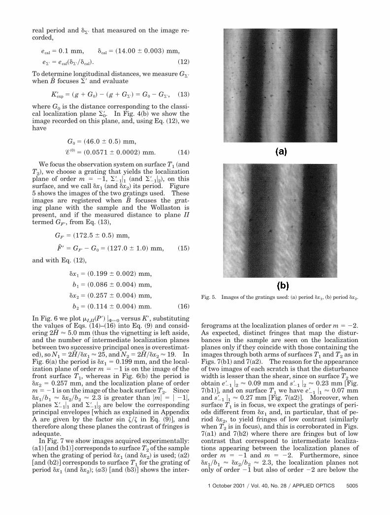
We focus the observation system on surface T1 �andT2�, we choose a grating that yields the localizationplane of order m � �1, ��1�1 �and ��1�2�, on thissurface, and we call �x1 �and �x2� its period. Figure5 shows the images of the two gratings used. Theseimages are registered when B focuses the grat-ing plane with the sample and the Wollaston ispresent, and if the measured distance to plane IItermed GF�, from Eq. �13�,

GF� � �172.5 � 0.5� mm,

F� � GF� � G0 � �127.0 � 1.0� mm, (15)

and with Eq. �12�,

�x1 � �0.199 � 0.002� mm,

b1 � �0.086 � 0.004� mm,

�x2 � �0.257 � 0.004� mm,

b2 � �0.114 � 0.004� mm. (16)

In Fig. 6 we plot �I,II�P�� 0 versus K�, substitutingthe values of Eqs. �14�–�16� into Eq. �9� and consid-ering 2H � 5.0 mm �thus the vignetting is left aside,and the number of intermediate localization planesbetween two successive principal ones is overestimat-ed�, so N1� 2H��x1� 25, and N2� 2H��x2� 19. InFig. 6�a� the period is �x1 � 0.199 mm, and the local-ization plane of order m � �1 is on the image of thefront surface T1, whereas in Fig. 6�b� the period is�x2 � 0.257 mm, and the localization plane of orderm��1 is on the image of the back surface T2. Since�x1�b1 � �x2�b2 � 2.3 is greater than �m� � � �1�,planes ��1�1 and ��1�2 are below the correspondingprincipal envelopes which as explained in AppendixA are given by the factor sin �� in Eq. �9�, andtherefore along these planes the contrast of fringes isadequate.

In Fig. 7 we show images acquired experimentally:�a1� and �b1� corresponds to surface T2 of the samplewhen the grating of period �x1 �and �x2� is used; �a2�and �b2� corresponds to surface T1 for the grating ofperiod �x1 �and �x2�; �a3� and �b3� shows the inter-

ferograms at the localization planes of order m��2.As expected, distinct fringes that map the distur-bances in the sample are seen on the localizationplanes only if they coincide with those containing theimages through both arms of surfaces T1 and T2 as inFigs. 7�b1� and 7�a2�. The reason for the appearanceof two images of each scratch is that the disturbancewidth is lesser than the shear, since on surface T2 weobtain e��1 �2 � 0.09 mm and s��1 �2 � 0.23 mm Fig.7�b1�, and on surface T1 we have e��1 �1 � 0.07 mmand s��1 �1 � 0.27 mm Fig. 7�a2�. Moreover, whensurface T1 is in focus, we expect the gratings of peri-ods different from �x1 and, in particular, that of pe-riod �x2, to yield fringes of low contrast �similarlywhen T2 is in focus�, and this is corroborated in Figs.7�a1� and 7�b2� where there are fringes but of lowcontrast that correspond to intermediate localiza-tions appearing between the localization planes oforder m � �1 and m � �2. Furthermore, since�x1�b1 � �x2�b2 � 2.3, the localization planes notonly of order �1 but also of order �2 are below the

Fig. 5. Images of the gratings used: �a� period �x1, �b� period �x2.


principal envelope of the degree of coherence, and theconstrast on these planes is such that, though lowerthan that for m � �1, it can enable fringes to beviewed �see Fig. 6�. Planes ��2 �1 and ��2 �2 are farfrom the images of the sample and, as expected, thefringes on them are straight. These fringes wereseen on the video monitor, but their contrast was solow that, to be able to show them in Fig. 7�a3� and7�b3� in the image processing program, we treatedthem with contrast and brightness different from therest.

In Table 1 we show the results corresponding tom��1 and m��2 for �x1 and �x2. We obtain thetheoretical values, K�m �theo and ��m� �theo, by replac-ing the results of Eqs. �14�–�16� in Eqs. �5� and �10�and considering q1 � 1. The experimental values,K�m �exp and ��m� �exp, are obtained when we measurethe values of G�� and use Eqs. �12�–�14�. The theo-retical and experimental results for K��1 differ by lessthan 3%, whereas those for ��1� by less than 0.6%.

Moreover, from Fig. 7 we see that the disturbancespresent in the sample are less than a wavelength andthat their profile could be evaluated from the inter-ferograms with Eq. �7�; however, this calculation isnot our purpose in the present paper.

4. Conclusion

A simple method for optically testing a transmissionsample with a few phase disturbances distributed inits volume is to place it in a two-beam interferometerilluminated by an extended periodic array of spatiallyincoherent sources. A layer can be tested when alocalization plane, different from the classical one, ismade to coincide with the plane containing its imagesthrough both arms of the interferometer. Differentlayers can be analyzed without moving either thesample or the interferometer but shifting the local-ization plane by a change in the source period. Inthe present paper the method has been applied to ashearing interferometer—a classical Wollastonprism—and the experimental results have corrobo-rated the theoretical predictions.

Appendix A: Multilocalization of Fringes

In an amplitude-division interferometer with twoarms, labeled I and II, there are two complementaryrepresentations,1 which we denote source and obser-vation representations. In the first there is a set ofplanes composed by the source and the two images ofthe observation plane back through arms I and II,while in the second the set of planes consists of theobservation plane and the two images of the sourcethrough the interferometer �Fig. 8�. In what followswe give a brief review of the multilocalization phe-nomenon that was analyzed in detail in our previouspaper.12

In the source plane there is an extended spatiallyincoherent source, �, and we define an orthogonalcoordinate system �x, y� with origin at the centralpoint, O, and an axis z perpendicular to �x, y�.12 Asource point of coordinates �x, y� is termed Sk, and thepoints on the upper and the lower borders of � aredenoted Su and Sd �and SdSu � 2H�. The images of�, O, Su, and Sd through arm I �and II� are termed ��,O�, S�u, and S�d �and ��, O�, S�u, and S�d�, respectively,and we have 2H� � S�uS�d �and 2H� � S�uS�d�.

In an arbitrary observation plane, ��, any of itspoints are termed P�, and its images back througharms I and II are PI and PII. In the particular casein which the observation plane is the classical local-ization one, ��0, the point is termed P�loc, and its im-ages are PI,loc and PII,loc. The rays OPII which herecoincides with OPII,loc �Ref. 12� and OPI subtend theangles "I and "II, respectively, with the x axis.Moreover, OPII,loc splits in the interferometer givingrise to rays “I” and “II”, whereas ray OPI originatesray “I”, which intersects “II” at point P�. The dis-

Fig. 6. Coherence patterns for �a� grating of period �x1 �b� gratingof period �x2.

Table 1. Longitudinal Distance and Fringe Spacing

m �x �mm� K� �exp �mm� K� �theo �mm� ��m� �exp ��m� ��m� �theo ��m�

�1 0.199 � 0.002 �29.3 � 0.9 �28.3 � 0.5 44.6 � 0.4 44.4 � 0.5�1 0.257 � 0.004 �23.0 � 0.9 �23.0 � 0.5 46.4 � 0.4 46.7 � 0.5�2 0.199 � 0.002 �48.5 � 1.0 �46.2 � 1.2 35.7 � 0.1 36.3 � 0.8�2 0.257 � 0.004 �41.6 � 1.0 �39.0 � 1.3 39.6 � 0.2 39.5 � 0.9


tance from P�loc to P� along ray “II” is termed Z�,and

Z� � P�locP�, F� � O�P�loc, F� � O�P�loc. (A1)

The differences in optical path lengths throughboth arms to an observation point P� are assumed tobe less than the coherence length, and the opticalpath lengths from the source point of coordinates �x,y� to P� along arms I and II are labeled LI�P�� and

Fig. 7. Images obtained experimentally with a periodic source: �a1� and �b1� correspond to surface T2 of the sample when thegrating of period �x1 �and �x2� is used; �a2� and �b2� correspond to surface T1 of the sample when the grating of period �x1 �and�x2� is used; �a3� and �b3� interferogram at the localization plane of order m � �2 when the grating of period �x1 �and �x2� isused.


LII�P��, respectively if the source point is O, we de-note the corresponding path lengths LI,O�P�� andLII,O�P��. The variation of optical path-length dif-ference for a fixed P� is

VOPD � LI�P�� LII�P�� LI,O�P�� LII,O�P��

� ��2��a10�P��x � a01�P��y

� ��x, y, P��, (A2)

where c is the velocity of light, a10�P�� 2�� #�LII�P�� LI�P��x$�x�y�0, a01�P�� 2�� #�LII�P�� LI�P��y$�x�y�0, and ��x, y, P�� is the

equivalent aberration. If the two beams leave theinterferometer in the same state of polarization, theintensity at P� is

I�P�� I�I��P�� I�II��P�� 2I�I��P��

� I�II��P��1�2��I,II�P��cos��P��, (A3)

��P�� being the phase at P�, which is such that

��P�� arg�I,II�P�� I,II � a00�P��, (A4)

where a00�P�� 2�� LII,O�P�� LI,O�P��, �I,II �a00�P�� is the phase difference at P� if point O alone

Fig. 8. Amplitude-division interferometer: P�loc �and P��, point at the classical localization �and at any observation� plane where ray “I”�and “I”� intersects “II”; PI,loc and PII,loc �or PI and PII�, images of P�loc �or P�� back through the interferometer. �a� Source space: O, centralsource point; Sd and Su, points on the lower and the upper borders of the source; �x, y, z�, orthogonal coordinates �z normal to the source�;"II and "I�"II�%", angles from the z axis to rays OPII and OPI; JI, point on the ray OPII,loc such that � � JIPI is parallel to x; n, refractiveindex. �b� Observation space: O� and O�, images of O through arms I and II; S�d and S�u, images of Sd and Su through arm I; �x�, y�, z��,coordinates at the source image through arm I �z� normal to S�dS�u�; Z�, distance from P�loc to P�; "�II, angle from the z� axis to the ray O�P�loc;J�, image of JI; � � � J�P�, relative coordinate; F� � O�P�loc; F� � O�P�loc; ��: bifurcation angle �from ray “II” to “I”�. n�, refractive index.


were present, and �I,II�P�� I,II�P��expi arg�I,II�P�� is the degree of coherence. For a periodicsource array of period �x consisting of N incoherentsources of width b parallel to the y axis, if the inter-ferometer has negligible aberrations, the constantcontrast condition holds, and there is translationsymmetry along the y axis,

�I,II�P��0 �1N

sin ��

sin��N�sin��

, (A5)

which is Eq. �31� of Ref. 12, where we have introducedthe symbols

� �ba10�P��

2�

n�b��

�sin "I � sin "II�

��q1b��0�

Z��F� � Z��

,

� ��xa10�P��

2�

n��x��

�sin "I � sin "II�

��q1�x

��0�

Z��F� � Z��

, (A6)

with

a10�P�� 2�n��

�sin "I � sin "II� �2�q1

��0�

Z��F� � Z��

,

��0� ��

n��F��d0�

��

n�1

��, q1 �

H� cos "�IIH

,

q �q1�x��0� , (A7)

where ��0� is the fringe spacing at ��0 �with d0�O�O��and "�II is the angle from the normal to �� to ray “I”.From Eq. �A5� the localization planes, termed ��m �mbeing an integer�, verify the multilocalization equa-tion, i.e., a10�P�m� � m2��x�. If "�II verifies theparaxial approximation and Z�m is the distance from��0 to ��m, then, in terms of variables of the observa-tion space, the multilocalization equation is Eq. �35�of Ref. 12

Z �m �F�m��0�

q1�x � m��0� with q1 �H�H

. (A8)

The normalized degree of coherence,�I,II�P�m� �� 0, is1 if m � 0 and less than 1 but larger than in otherregions if m � 0. The fringe spacing at ��m Eq. �37�of Ref. 12 is

��m� ��F� � Z �m��

n��d0�� 0��1 �

Z �mF� � �

��0�

1 � m�q. (A9)

Between two successive planes ��m there are N � 2intermediate localization planes of much lower con-trast and such that sin��N��N sin�� 1�#Nsin�k � 1�2��N$ �with k integer and k�N not inte-ger� and there are N � 1 planes with no contrast.The fringe localization depth of ��m is defined as the

distance between the two adjacent regions of zerocontrast at both sides of ��m, and from Eq. �39� of Ref.12 it is

L.D. �m � Z �m�1�N � Z �m�1�N

�2F�

Nq�1 � m�q�2 � 1��Nq�. (A10)

Moreover, the coherence pattern is modulated by en-velopes factor sin �� in Eq. �A5�, the principal onehas peak at ��0, and the maxima below it verify �m� ��x��b.

Appendix B: Interferometer Parameters

For a two-beam interferometer, the central point ofan observation plane, ��, is termed P�o, and its imagesthrough arms I and II by inverse ray tracing are PIoand PIIo. The parameters shear, shift, delay, tilt,and lead have been defined by Steel for the generalcase,1 and here we consider the unidimensional case�Fig. 9�. In the source representation, the two im-ages of �� back through arms I and II, ��I� and ��II�,are inclined to each other at the angle of tilt &o, andthe rays OPIo and OPIIo are such that the distanceOPIo � OPIIo � ho is the shift and their lateral sep-aration is the shear so. The shear depends on theplane �� considered, and, in the general case, it alsovaries from one point P� of �� to another, but, if it isindependent of P�, it is said to be lateral. The delayis 'o � �OP�oII � OP�oI��c. In the observation rep-resentation, O�P�o and O�P�o are such that their lateralseparation is the tilt t�o, whereas O�P�o � O�P�o � l�o isthe lead.

Under the approximations of Subsection 2.A, theshift is zero and the shear in the source and obser-vation representations are so � PIIoPIo and s�o � B�B�� oK�, respectively �K� is the distance from theclassical localization plane ��0 to ��. If the observa-tion plane is ��0, then in the source representation,only one ray is emitted by O to originate the two raysthat intersect at P�loc, so s�0� � 0, and, in the observa-tion representation, K� � 0 and s��0� � 0. For any ��,the shear in the source and observation representa-tions, so and s�o, are related, since, from Eqs. �1� and

Fig. 9. Interferometer parameters: O, central source point; PIo

and PIIo, images of the observation point P�o back through the twoarms; ��I� and ��II�, images of �� back through the two arms; �� and��, images of the effective source � through arms I and II; &o, angleof tilt; OPIo � OPIIo � ho, shift; so, shear; 'o � �OP�oII � OP�oI��c,delay; t�o, tilt; O�P�o � O�P�o � l�o, lead.


�A7� and from Fig. 1, assuming "I and "II small andwriting �sin "I � sin "II� � so�D, q1 � H��H and��0� � ��n��,

n � H �so

D� n� � H� �

s�oD�

, (B1)

which is invariant for the interferometer �i.e., eten-due in the bidimensional case�.1

This research was performed with the support ofConsejo Nacional de Investigaciones Cientificas yTecnicas �CONICET� and Universidad de BuenosAires �UBA�. We are grateful to Ezequiel Carbon forthe figures.

References1. W. H. Steel, Interferometry �Cambridge University, London,

1967�.2. P. Hariharan, B. F. Oreb, and T. Eiju, “Digital phase-shifting

interferometry: a simple error-compensating phase calcula-tion algorithm,” Appl. Opt. 26, 2504–2506 �1987�.

3. D. W. Phillion, “General methods for generating phase-shiftinginterferometry algorithms,” Appl. Opt. 36, 8098–8115 �1997�.

4. D. Malacara, M. Servin, and Z. Malacara, Interferogram Anal-ysis for Optical Testing �Marcel Dekker, New York, 1998�.

5. B. V. Dorrio and J. L. Fernandez, “Phase-evaluation methods

in whole-field optical measurement,” Meas. Sci. Technol. 10,33–55 �1999�.

6. J. M. Simon and S. A. Comastri, “Localization of interferencefringes,” Am. J. Phys. 48, 665–668 �1980�.

7. J. M. Simon and S. A. Comastri, “Fringe localization depth,”Appl. Opt. 26, 5125–5129 �1987�.

8. J. M. Simon and S. A. Comastri, “Interferometers: equivalentsine condition,” Appl. Opt. 27, 4725–4730 �1988�.

9. S. Cha and C. M. Vest, “Interferometry and reconstruction ofstrongly refracting asymmetric-refractive-index fields,” Opt.Lett. 4, 311–313 �1979�.

10. J. Jahns and A. W. Lohmann, “The Lau effect �a diffractionexperiment with incoherent illumination�,” Opt. Commun. 28,263–267 �1979�.

11. J. M. Simon, M. C. Simon, R. M. Echarri, and M. T. Garea,“Fringe localization in interferometers illuminated by a suc-cession of incoherent line sources,” J. Mod. Opt. 45, 2245–2254�1998�.

12. S. A. Comastri and J. M. Simon, “Multilocalization and vanCittert–Zernike theorem. 1. Theory,” J. Opt. Soc. Am. 17,1265–1276 �2000�.

13. J. M. Simon and S. A. Comastri, “Multilocalization and vanCittert–Zernike theorem. 2. Application to the Wollastonprism,” J. Opt. Soc. Am. 17, 1277–1283 �2000�.

14. J. M. Simon, S. A. Comastri, and R. Echarri, “The Mach–Zehnder interferometer: examination of a volume by non-classical localization plane shifting,” Pure Appl. Opt. 3, 242–249 �2001�.


Shifting of Localization Planes in Optical Testing: Application to a Shearing Interferometer

Documents

Transcript of Shifting of Localization Planes in Optical Testing: Application to a Shearing Interferometer