Sharp-interface simulation of dendritic growth with convection: benchmarks
13
Sharp-interface simulation of dendritic growth with convection: benchmarks H.S. Udaykumar * , S. Marella, S. Krishnan Department of Mechanical and Industrial Engineering, 4116 Seamans Center for the Engineering Arts and Science, University of Iowa, Iowa City, IA 52242-1527, USA Received 14 August 2002; received in revised form 12 December 2002 Abstract We present and validate a numerical technique for computing dendritic growth of crystals from pure melts in the presence of forced convection. The Navier–Stokes equations are solved on a fixed Cartesian mesh and a mixed Eulerian–Lagrangian framework is used to treat the immersed phase boundary as a sharp solid–fluid interface. A conservative finite-volume discretization is employed which allows the boundary conditions to be applied exactly at the moving surface. Results are presented for a range of the growth parameters, namely crystalline anisotropy, flow Reynolds number and Prandtl number. Direct comparisons are made between the present results and those obtained with phase-field methods and excellent agreement is obtained. Values for the tip characteristics are tabulated to serve as benchmarks for computations of two-dimensional dendritic growth with convection. Ó 2003 Elsevier Science Ltd. All rights reserved. 1. Introduction A method for computing the evolution of dendritic phase boundaries on fixed Cartesian grids is presented. The effect of imposed forced convection on the dendrite tip morphology is investigated. The phase front is trea- ted as a sharp boundary that runs through the mesh and a conservative finite-volume method is applied for so- lution of the Navier–Stokes equations. The numerical solutions are validated against available [1–4] two- dimensional dendritic growth solutions under the effect of forced convection. In previous work [5] we described a finite-difference technique for simulation of diffusion-controlled growth of unstable phase boundaries. For the case of dendritic solidification of pure materials from the melt, we dem- onstrated that a sharp interface approach can be de- veloped that yields globally second-order accurate solutions to the field equations. The interface position was computed with first-order accuracy. In subsequent work [6,7], we devised a finite-volume approach for solving the incompressible Navier–Stokes equations to compute incompressible flows around fixed and moving immersed solid bodies. This paper combines the capability to evolve den- dritic phase boundaries presented in Ref. [5] with the Navier–Stokes solver in Ref. [7]. As in the case of the Navier–Stokes solutions presented in the latter refer- ence, fluxes (of heat in the present case) are explicitly conserved across the control volume faces. Using a compact linear-quadratic interpolant [5] to evaluate the fluxes at the control volume faces that are cut by the immersed interface, a second-order accurate flux evalu- ation procedure is devised. Various techniques, including phase-field [1–3,10,11], level-sets [12–14], finite-elements [15,16], and finite-dif- ference front-tracking [5,17], have been employed to simulate dendritic solidification. The phase-field method is currently the most popular approach and was the first approach used [2,3] to determine whether the quantita- tive measures, such as tip radius, velocity and the se- lection parameter of the numerically grown dendrites could be validated against microscopic solvability the- ory. This method has also been used to study the be- havior of dendrite tips under the influence of forced * Corresponding author. Tel.: +1-319-384-0832; fax: +1-319- 335-5669. E-mail address: [email protected] (H.S. Udaykumar). 0017-9310/03/$ - see front matter Ó 2003 Elsevier Science Ltd. All rights reserved. doi:10.1016/S0017-9310(03)00038-3 International Journal of Heat and Mass Transfer 46 (2003) 2615–2627 www.elsevier.com/locate/ijhmt
Transcript of Sharp-interface simulation of dendritic growth with convection: benchmarks

Sharp-interface simulation of dendritic growthwith convection: benchmarks
H.S. Udaykumar *, S. Marella, S. Krishnan
Department of Mechanical and Industrial Engineering, 4116 Seamans Center for the Engineering Arts and Science,
University of Iowa, Iowa City, IA 52242-1527, USA
Received 14 August 2002; received in revised form 12 December 2002
Abstract
We present and validate a numerical technique for computing dendritic growth of crystals from pure melts in the
presence of forced convection. The Navier–Stokes equations are solved on a fixed Cartesian mesh and a mixed
Eulerian–Lagrangian framework is used to treat the immersed phase boundary as a sharp solid–fluid interface. A
conservative finite-volume discretization is employed which allows the boundary conditions to be applied exactly at the
moving surface. Results are presented for a range of the growth parameters, namely crystalline anisotropy, flow
Reynolds number and Prandtl number. Direct comparisons are made between the present results and those obtained
with phase-field methods and excellent agreement is obtained. Values for the tip characteristics are tabulated to serve as
benchmarks for computations of two-dimensional dendritic growth with convection.
� 2003 Elsevier Science Ltd. All rights reserved.
1. Introduction
A method for computing the evolution of dendritic
phase boundaries on fixed Cartesian grids is presented.
The effect of imposed forced convection on the dendrite
tip morphology is investigated. The phase front is trea-
ted as a sharp boundary that runs through the mesh and
a conservative finite-volume method is applied for so-
lution of the Navier–Stokes equations. The numerical
solutions are validated against available [1–4] two-
dimensional dendritic growth solutions under the effect
of forced convection.
In previous work [5] we described a finite-difference
technique for simulation of diffusion-controlled growth
of unstable phase boundaries. For the case of dendritic
solidification of pure materials from the melt, we dem-
onstrated that a sharp interface approach can be de-
veloped that yields globally second-order accurate
solutions to the field equations. The interface position
was computed with first-order accuracy. In subsequent
work [6,7], we devised a finite-volume approach for
solving the incompressible Navier–Stokes equations to
compute incompressible flows around fixed and moving
immersed solid bodies.
This paper combines the capability to evolve den-
dritic phase boundaries presented in Ref. [5] with the
Navier–Stokes solver in Ref. [7]. As in the case of the
Navier–Stokes solutions presented in the latter refer-
ence, fluxes (of heat in the present case) are explicitly
conserved across the control volume faces. Using a
compact linear-quadratic interpolant [5] to evaluate the
fluxes at the control volume faces that are cut by the
immersed interface, a second-order accurate flux evalu-
ation procedure is devised.
Various techniques, including phase-field [1–3,10,11],
level-sets [12–14], finite-elements [15,16], and finite-dif-
ference front-tracking [5,17], have been employed to
simulate dendritic solidification. The phase-field method
is currently the most popular approach and was the first
approach used [2,3] to determine whether the quantita-
tive measures, such as tip radius, velocity and the se-
lection parameter of the numerically grown dendrites
could be validated against microscopic solvability the-
ory. This method has also been used to study the be-
havior of dendrite tips under the influence of forced
*Corresponding author. Tel.: +1-319-384-0832; fax: +1-319-
335-5669.
E-mail address: [email protected] (H.S. Udaykumar).
0017-9310/03/$ - see front matter � 2003 Elsevier Science Ltd. All rights reserved.
doi:10.1016/S0017-9310(03)00038-3
International Journal of Heat and Mass Transfer 46 (2003) 2615–2627
www.elsevier.com/locate/ijhmt

convection [4]. The phase-field method falls under the
class of Eulerian (i.e. fixed grid) methods called ‘‘diffuse
interface’’ methods [18]. In such methods the interface is
not a sharp phase boundary but is given a certain
thickness or spread on the computational mesh. Typi-
cally, the interface thickness occupies a few mesh cells. A
front-tracking method for the case of dendritic growth
with convection has also been presented in [30]. How-
ever, the treatment of the solid–liquid front in the so-
lution of the governing equations is not sharp as in the
present work.
To our knowledge, the present work represents the
first sharp interface simulations of dendritic growth in
the presence of convection. While the interface is tracked
in this work using markers and curves the approach can
use other, more versatile interface representations that
permit treatment of the boundaries as sharp entities,
such as level-set methods [12]. This is being done in
ongoing work using level-sets to track the interface. The
present work places the finite-volume sharp interface
approach on sound footing by directly comparing the
results of the computations with results from the often
used phase-field approach [4,8]. The method is shown to
predict the correct physical behavior in the dendritic
growth of pure materials. This validation effort aug-
ments the demonstration of grid size and orientation
independence and convergence studies for the sharp in-
terface method for dendritic growth in the diffusion-
limited regime, presented in Udaykumar et al. [9]. These
solutions provide benchmarks for calculations of den-
drite tips growing in the presence of axially directed
forced convection.
2. Solvability theory and convection effect
Microscopic solvability is the currently accepted
theory for the growth of dendritic structures in solidifi-
cation from the melt. Extensive reviews on the subject
are available (e.g. [19]). Bouissou and Pelce [22] devel-
oped the solvability theory including convective effects
on dendrites, using an Oseen flow solution under the
assumptions of: (a) uniform flow at velocity U1 directed
along an axis of the dendrite, (b) an isothermal tip and
(c) the tip as a paraboloid of revolution. They obtained
the solution for the translating paraboloid which pro-
vides the steady-state tip radius (qt) and tip velocity (Vt)as:
D ¼ Pet expðPet � PefÞ
�Z 1
1
f�Petg þ Pefb2þR g1
gð1Þffiffi1
p d1 � gcgffiffiffig
p dg ð1Þ
where D is the undercooling, Pet the tip Peclet num-ber¼ Vtqt=2a, Pef is the flow Peclet number¼U1qt=2a,Re is the Reynolds number¼ðU1qtÞ=m ¼ ð2PefÞ=Pr
where a is the thermal diffusivity, m is the kinematicviscosity and e is the anisotropy parameter. The functiongðfÞ is given by:
gð1Þ ¼ ffiffiffi1
p erfcðffiffiffiffiffiffiRe
p1=2Þ
erfcðffiffiffiffiffiffiffiffiffiffiRe=2
pÞþ
ffiffiffiffiffiffiffiffiffiffiffiffiffiffiffiffiffi2=ðpReÞ
perfcð
ffiffiffiffiffiffiffiffiffiffiRe=2
pÞ
� ½expð�Re=2Þ � expð�Re1=2Þ�
The above expressions reduce to the Ivantsov solution
[20] for the no-flow case. The primary result from the
solvability theory with convection is that the selection
parameter for the case with flow (r�) is related to the
value in the absence of flow ðr�0 ¼ ð2ad0Þ=ðq2t VtÞÞ,
through:
r�0
r� ffi 1þ bv11=14 for v � 1;
while
r�0
r� ffi 1 for v � 1 ð2Þ
where the capillary length d0 ¼ ðc0TmCpÞ=L2, and theparameters v ¼ ðaðReÞd0U1Þ=ðb3=4qtVtÞ, b ¼ 15e and
aðReÞ ¼ffiffiffiffiffiffiffiffiffiffiffiffiffi2Re=p
pexpð�Re=2Þerfc
ffiffiffiffiffiffiffiffiffiffiRe=2
p. In the present
case the Reynolds numbers are low, so that the v � 1
situation holds. In this limit the selection parameter
should change little from the no-flow case.
3. Governing equations
To test the numerics, we grow a dendritic front for
specified control parameters, namely the undercooling
(D), capillary length (d0), anisotropy strength (�) andimposed flow strength measured by the non-dimensional
velocity U1d0=al. The predicted selection parameter (r�)
and selected tip radius (qt) and velocity (Vt) are thencompared with the results of solvability theory and with
the diffuse-interface results obtained from phase-field
method [4,8]. The following non-dimensional quantities
are used: length x ¼ X=d0, time s ¼ tal=d20 , velocity~uu ¼ ð~UUd0Þ=al, and temperature H ¼ ðT � TmÞ=ðL=CpÞ.The incompressible Navier–Stokes equations are
solved:
r �~uu ¼ 0 ð3Þ
o~uuos
þ~uu � r~uu ¼ �rp þ Prr2~uu ð4Þ
Pr is the Prandtl number¼ ml=al where m is the kinematicviscosity, subscript l stands for the liquid phase. The
heat conduction equation is solved in the solid and liq-
uid phases separately, in non-dimensional form:
oHos
þ~uu � rH ¼ a�l=sr2H ð5Þ
In the above the convective term applies in the solid
phase, the variable a�l=s ¼ al=s=al is the non-dimensional
2616 H.S. Udaykumar et al. / International Journal of Heat and Mass Transfer 46 (2003) 2615–2627

diffusivity only, and subscript l/s indicates the phase
(liquid or solid). The interface temperature equation is
written in non-dimensional form:
Hi ¼ �dðhÞj ð6Þ
where j is the interfacial curvature and the capillarityparameter is prescribed using the model [13] and
dðhÞ ¼ d0ð1� 15e cos 4hÞ ð7Þ
For phase change of pure materials the normal velocity
at a point on the front is provided by the rate of
transport of latent heat away from the solid–liquid
interface (Stefan condition). In non-dimensional form,
this equation is:
Vi ¼oHon
� �s
�� oH
on
� �l
�ð8Þ
where subscripts s and l apply to solid and liquid re-
spectively and n represents the direction normal to the
interface. Note that the boundary conditions at the
farfield (at large distance r from the origin) for a crystalgrowing in the undercooled melt with a uniform flow
directed toward the dendrite tip then become:
Hðr ! 1; sÞ ¼ �D ð9aÞ
uðr ! 1; sÞ ¼ U1d0al
ð9bÞ
4. Numerical method
4.1. Interface tracking
The interface is tracked using markers connected by
piecewise quadratic curves parametrized with respect to
the arclength. Details regarding interface representation,
evaluation of derivatives along the interface to obtain
normals, curvatures etc. have been presented in previous
papers [5,7] and are not repeated here. Also described in
earlier papers are details regarding the interaction of the
interfaces with the underlying fixed Cartesian mesh.
These include obtaining locations where the interface
cuts the mesh, identifying phases in which the cell cen-
ters lie, and procedures for obtaining a consistent mosaic
of control volumes in the cells [6].
4.2. Flow solver
The fractional step scheme [24] is used for advancing
the fluid flow solution in time. The Navier–Stokes
equations are discretized on the Cartesian mesh using a
cell-centered collocated (non-staggered) arrangement of
the primitive variables (~uu; p). The integral forms of thenon-dimensionalized governing equations are used as
the starting point:
I~uu �~nndS ¼ 0 ð10Þ
o
os
Z~uudV þ
I~uuð~uu � n̂nÞdS
¼ �I
p~nndS þ PrI
r~uu � n̂ndS ð11Þ
where~nn is a unit vector normal to the face of the controlvolume. The above equations are to be solved with
~uuð~xx; tÞ ¼~uuoð~xx; tÞ on the boundary of the flow domainwhere ~uuoð~xx; tÞ is the prescribed boundary velocity, in-cluding that at the solid–liquid interface. A second-order
accurate, two-step fractional step method is used [6]. A
second-order Adams-Bashforth scheme is employed for
the convective terms and the diffusion terms are dis-
cretized using an implicit Crank-Nicolson scheme. In
addition to the cell-center velocities, which are denoted
by ~uu, we also introduce face-center velocities ~uuf . In amanner similar to a fully-staggered arrangement, only
the component normal to the cell-face is computed and
stored. The face-center velocity is used for computing
the volume flux from each cell in the finite-volume dis-
cretization scheme. The advantage of separately com-
puting the face-center velocities has been discussed in the
context of the current method in [6]. The semi-discrete
form of the advection-diffusion equation for each cell
can therefore be written as follows:
Zv
~uu� �~uun
dsdV ¼ � 1
2
I½3~uunð~uunf �~nnÞ �~uun�1ð~uun�1f �~nnÞ�dS
þ Pr2
Iðr~uun þr~uu�Þ � n̂ndS ð12Þ
where ~uu� is the intermediate cell-center velocity. Theadvection-diffusion step is followed by the pressure-
correction step:
Zv
~uunþ1 �~uun
dtdV ¼ �
Zvrpnþ1 dV ð13Þ
By requiring a divergence-free velocity field at the end of
the time-step we get the equation for pressure,
Irpnþ1 dS ¼ 1
dt
I~uu�f �~nndS ð14Þ
which is the weak form of the pressure Poisson equation.
Once the pressure is obtained by solving this equation,
both the cell-center and face-center velocities, ~uu and ~uufare updated separately as follows:
~uunþ1 ¼~uu� � dtðrpnþ1Þcc ð15Þ
~uunþ1f ¼~uu�f � dtðrpnþ1Þfc ð16Þ
where subscripts cc and fc indicate evaluation at the cell
center and face center locations respectively.
H.S. Udaykumar et al. / International Journal of Heat and Mass Transfer 46 (2003) 2615–2627 2617

The energy equation, is written in semi-discrete form
as:Zv
Hnþ1 � Hn
dtdV ¼ � 1
2
I½3Hnð~uunf �~nnÞ � Hn�1ð~uun�1f �~nnÞ�dS
þ al=s2
IðrHnþ1 þrHnÞ � n̂ndS ð17Þ
The above Crank–Nicolson scheme provides nominal
second-order temporal accuracy.
In discrete form Eq. (17) is written, for a control
volume in the Cartesian mesh indexed (i; j) as:
DVijdt
ðHnþ1ij � Hn
ijÞ ¼al=s2
X5f¼1
oHon
nþ1�þ oH
on
n �f
DSf
� 12
X5f¼1
½3Hnð~uunf �~nnÞ
� Hn�1ð~uun�1f �~nnÞ�DSf ð18Þ
The fluxes at control volume faces are evaluated by
constructing a compact two-dimensional polynomial
interpolating function [6] from available neighboring
cell-center values, which gives a second-order accurate
approximation of the fluxes and gradients on the faces
of the trapezoidal boundary cells. This interpolation
scheme coupled with the finite-volume formulation
guarantees that the accuracy and conservation property
of the underlying algorithm is retained even in the
presence of arbitrary-shaped immersed boundaries.
The discrete equations are solved using the standard
line-SOR procedure, with alternate sweeps in the i- andj-directions and a standard Thomas algorithm for the
solution of the resulting tri-diagonal matrix. The use of a
Cartesian grid allows for the use of these fast solution
procedures. The discretization of the fluid velocity and
pressure Poisson equations has been described in detail
in previous papers [7]. A multigrid method is used for
fast solution of the pressure Poisson equation.
4.3. Computing the interface velocity
The interface velocity is obtained as described in [5].
The temperature gradient in each phase is obtained by
the normal probe technique, where a normal from the
interface marker is extended into each phase. The tem-
perature values at two nodes on the normal, placed at
distances equal to the local mesh spacing dx, are ob-tained from the background mesh by bilinear interpo-
lation. Second-order accuracy of this technique has been
demonstrated in Udaykumar et al. [5]. The gradient is
then obtained as:
oHon
¼ 4Hn1 � Hn2 � 3Hint
2dxð19Þ
where subscripts n1 and n2 imply evaluations of tem-perature at the two nodes on the normal probe and
subscript int implies the value on the interface. Having
calculated the temperature gradients in each phase using
Eq. (19), the interface velocities are computed at the
markers using Eq. (8). These are then advected to new
positions in order to evolve the interface in time.
4.4. Overall solution procedure
For curvature-driven growth problems, stability of
the interface update requires an implicit coupled pro-
cedure for obtaining the field solution [26,27] and the
interface position simultaneously at time level tnþ1. Inthe absence of an implicit, coupled treatment of the field
solution and interface evolution, the calculations can
become very stiff. The stability restriction on an explicit
scheme can be very severe (dt ¼ Oðdx3Þ) as demon-strated by Hou et al. [26]. However, solving for the fluid
flow equations, particularly the pressure Poisson equa-
tion iteratively over each time step would be computa-
tionally taxing. Moreover, the interface shape couples
directly with the temperature field through the Stefan
and Gibbs–Thomson condition and only indirectly to
the fluid flowfield through its effect on the thermal field.
Therefore, within a time step we only couple the tem-
perature field and interface update in an iterative fashion
while updating the velocity and pressure fields in the
usual manner outside the iteration loop.
An implicit procedure similar to that employed in [5]
is used. The overall solution procedure with boundary
motion is as follows:
(0) Advance to next time step t ¼ t þ dt. Iteration coun-ter k ¼ 0.
(1) Update the interface position. Determine the inter-
section of the immersed boundary with the Carte-
sian mesh. Using this information, reshape the
boundary cells.
(2) Solve the fluid flow and pressure Poisson equations.
Correct the velocity field to satisfy zero-divergence.
(3) Augment iteration counter, k ¼ k þ 1.(4) Determine the intersection of the immersed bound-
ary with the Cartesian mesh. Using this information,
reshape the boundary cells. For each reshaped
boundary cell, compute and store the coefficients
appearing in discrete form for the energy equation,
Eq. (18).
(5) Advance the discretized heat equation in time to ob-
tain Hkij.
(6) Advance the interface position in time.
(7) Check whether the temperature field and interface
have converged.
Convergence is declared if: max jHkij � Hk�1
ij j < eTand max jXk
ip � Xk�1ip j < eI, where k is the iteration
number and � is a convergence tolerance set to 10�5
in the calculations so that the solution obtained is
independent of the convergence criterion.
2618 H.S. Udaykumar et al. / International Journal of Heat and Mass Transfer 46 (2003) 2615–2627

(8) If not converged, go to step 3 for next iteration. If
converged, go to step 0 for next time step.
Typically, less that five iterations of the heat equation
and interface update are required for convergence since
the previous time step solution provides an excellent
guess to the solution at the current step. Note that with
this implicit iterative approach stable computations of
interface evolution can be performed with time-step sizes
that are controlled by a CFL-type criterion of the form
dt ¼ kdx=maxðVinterface;UflowÞ, where k is set to 0.1 in thecalculations performed.
4.5. Computational setup
The numerical method described above is now used in
computations of dendritic growth and is shown to pro-
vide physically correct solutions for dendritic growth of
crystals. It will be shown that the effects of all the control
parameters, namely undercooling (D), anisotropy (e) andimposed flow strength (U1d0=al) are correctly capturedby the algorithm. The results are compared quantita-
tively with results from the phase-field approach and
qualitatively with the solvability theory.
To start the computations, a semi-circular seed
crystal is placed at the origin of the computational do-
main of dimension ð0:5HÞ � ðHÞ. Symmetry across they-axis is exploited to solve in the half-space. In calcu-
lations below, we adopt H ¼ 2000. The initial radius ofthe seed is 15 non-dimensional units (i.e. 15 capillary
lengths in dimensional terms) and it is placed with its
center at (0,1000). A uniform fine mesh is placed in an
inner region, as shown in Fig. 1, while the mesh is
coarsened linearly from the edge of the fine mesh region
to the end of the domain. We have shown in earlier work
[5], that the sharp interface approach gives solutions for
dendritic growth that are independent of the mesh
spacing and mesh orientation. In the following we
compare the results of solutions that were deemed grid
independent by performing a series of calculations on
progressively refined grids for the case shown in Fig. 2,
until the steady-state results on two successive grid sizes
were found to agree adequately with each other (to
within a few percent for the tip radius and velocity).
The computations are performed starting from an
initial condition supplied to be H ¼ 0 in the solid seedand H ¼ �D, the nondimensional undercooling value,elsewhere in the domain. Since this initial temperature
field is discontinuous at the interface, the interface ve-
locity in the initial stage of the calculations will be very
large. To avoid problems with stability due to the large
value of velocity, the seed is held in place (i.e. interface
velocity is set to zero) for the first hundred time steps of
the calculation. This allows a thermal boundary layer of
the extent of a few mesh spacings to form around the
seed. Thereafter the seed is allowed to grow with the
velocity computed from Eq. (8). Although these initial
conditions are somewhat arbitrary, the evolution of the
dendrite to the desired theoretical tip shape appears to
proceed regardless of the initial condition, providing a
strong indication that the tip selection mechanism op-
erates early in the growth of the dendrite. Computations
are carried out until the tip velocity, radius and selection
parameter have each hit steady-state values. The time
required to achieve steady-state depends on the param-
eters assigned for each case and a typical trend is shown
in Fig. 3(a) for the case with D ¼ 0:55, d0 ¼ 0:5 and� ¼ 0:03. The non-dimensional tip velocity, Vtd0=al, tipradius qt and selection parameter r� are shown in the
figure with appropriate multipliers to fit all the curves on
Fine Mesh
Coarse Mesh
Symmetry Line
Inlet
Outlet
Symmetry Line
-=
u8 = U d0 /α l
Nucleus
∆Θ
8
Fig. 1. Illustration of the computational set-up for the simulation of dendritic growth with flow.
H.S. Udaykumar et al. / International Journal of Heat and Mass Transfer 46 (2003) 2615–2627 2619

the same plot. The selection parameter appears to be
established very quickly in the growth process. The ve-
locity and tip curvature then adjust in time until they
approach steady-state values. This was found to be an
interesting common aspect in the computations of den-
dritic growth for the range of parameters explored in
this study. It appears that the pattern selection mecha-
nism that determines r� operates in the entire growth
process, even in the earlier stages of the growth, while
the radius and velocity of the tip are ‘‘driven’’ towards
appropriate values to yield the established r�. These
observations are consistent with those of Plapp and
Karma [29].
5. Results
The dendritic solidification calculations using the
current approach has been validated against solvability
theory in a previous paper [9]. Issues such as order of
accuracy have been addressed in the context of solidifi-
cation in Udaykumar et al. [5] and for the Navier–
Stokes equations for stationary and moving boundaries
in Ye et al. [6] and Udaykumar et al. [7] respectively. In
this paper, we compare our results with those from the
phase-field method as presented in Tong et al. [4]. Tong
et al. [4] and Tong [8] in turn have shown that their
results are in agreement with predictions of morpho-
logical solvability theory under certain assumptions
which we will point out later in this section.
In Fig. 2 we show the dendritic growth computed in a
half-space for purely diffusive transport. This case cor-
responds to D ¼ 0:55, e ¼ 0:03, m ¼ 4, i.e. four-foldanisotropy. In the following calculations we maintain
the capillarity parameter d0 ¼ 0:5. The y-axis is a sym-
metry line. Only a part of the domain is shown. Grid
refinement studies were performed to ensure that the
result shown is independent of grid resolution.
The tip characteristics for this case were shown to
agree with solvability theory in Udaykumar et al. [9]. In
Fig. 2(a) we show successive shapes of the evolving
dendrite until steady-state dendrite growth is reached.
Fig. 2(b) shows the isotherms in the solid and liquid
phases. The contours in the solid represent the effects of
interface curvature since, in the absence of temperature
variations on the interface arising from the Gibbs–
Thomson effect, the temperature in the solid would have
been uniformly equal to the melting temperature (i.e.
H ¼ 0).Fig. 3 shows the effect of convection on dendritic
growth for D ¼ 0:55, e ¼ 0:03, m ¼ 4. These are thesame parameters as for Fig. 2. In the case of Fig. 3
however, a flowfield is imposed. The non-dimensional
flow strength at the farfield u1 ¼ 0:0675. Fig. 3(a) showsthe behavior of the tip with time. The tip velocity, radius
and selection parameter are all shown in Fig. 3(a), with
appropriate multipliers to clarify the plot. The tip of
interest is the one facing the oncoming flow. The tip
characteristics quickly approach steady-state values.
Towards the end of the time duration for which this
dendrite tip was computed, the tip is approaching the
edge of the fine mesh region and hence the tip charac-
teristics begin to deviate slightly from the steady-state
values. The dendrite shapes at different instants in the
approach to steady-state are plotted in Fig. 3(b). The
temperature contours are shown in Fig. 3(c). Note that,
in contrast to the shapes and temperature fields in Fig. 2,
in this case convection introduces a fore-aft asymmetry.
The tip facing the oncoming flow grows much faster
than the one downstream due to the thinner thermal
Fig. 2. Dendrite solutions for the case without flow, D ¼ 0:55, e ¼ 0:03. (a) Dendrite shape evolution with time. (b) Temperaturecontours around the dendrite for the final shape in (a).
2620 H.S. Udaykumar et al. / International Journal of Heat and Mass Transfer 46 (2003) 2615–2627

boundary layer at the front of the dendrite. The tip that
grows laterally also grows fairly rapidly, in fact at a rate
that is close to the diffusion-driven growth velocity
[4,22,25]. However this tip is asymmetric across the tip
axis since the thermal boundary layer on the upstream
side is thinner than that on the downstream side. It is
noticed that the tip that is downstream does not achieve
a steady-state, at least for the duration of the compu-
tations shown. Therefore the most natural choice for
comparison and analysis is the upstream tip. In Fig. 3(d)
and (e), we show the velocity field and pressure contours
around the dendrite for the final (steady-state) shape
shown in Fig. 3(b). A zoomed-in view is also shown near
the tip that grows laterally. These figures show that the
present sharp-interface technique computes the velocity
and pressure fields around the dendrite in a smooth
fashion and that the no-slip boundary condition is ap-
plied in a sharp manner thus capturing the boundary
layer without smearing.
The effect of crystalline anisotropy is shown in Fig. 4.
Fig. 4(a) corresponds to e ¼ 0:01 and Fig. 4(b) toe ¼ 0:05. The flow is at u1 ¼ 0:0675, the same value asin Fig. 3. The dendrites are evolved until a steady-state
upstream tip is reached. The influence of anisotropy in
sharpening the tip is clearly seen in the figures. Quanti-
tative aspects of these dendrite tips will be discussed
later. In Fig. 5 we show the evolution of the tip with
D ¼ 0:55, e ¼ 0:03, m ¼ 4 and u1 ¼ 0:14, i.e. twice theflow strength compared to the case in Fig. 4. The effect
of the enhanced convection on the dendrite tip appears
to be imperceptible in the shape of the dendrite. Al-
though the thermal field shows some enhancement of the
fore-aft asymmetry due to the increased strength of the
flow, the differences between Figs. 3(c) and 5(b) are
small. The tip characteristics are also seen (Tables 1 and
2) to change only mildly. The variation in the tip velocity
and tip radius for flow strengths lower than 0.0675 is
quite significant as see from Table 2 and Fig. 7. There
Fig. 3. Dendrite solutions for forced flow with U1 ¼ 0:0675, e ¼ 0:03, D ¼ 0:55. (a) The tip characteristics of the dendrite and theapproach to steady-state tip behavior. (b) Evolution of the shape of the dendrite. (c) Temperature contours around the dendrite. (d)
Pressure contours and velocity vectors around the dendrite. (e) Close-up of the pressure contours and the velocity vectors around the
tip growing in the +x-direction.
H.S. Udaykumar et al. / International Journal of Heat and Mass Transfer 46 (2003) 2615–2627 2621

appears to be a lowering of the slopes of the Vt againstu1 and qt against U1 curves. This behavior has been
shown in the phase-field study by Tong [8]. The tip ve-
locity and radius appear to saturate as the u1 increases.The Prandtl number in all of the above cases was
23.1, a value corresponding to the popular organic
model material succinonitrile [21]. In Fig. 6 we compare
the results for Pr ¼ 23:1 with that for Pr ¼ 0:01, thislatter value being more representative of metallic melts.
Fig. 6(a) shows the evolution and temperature field for
Pr ¼ 23:1 and u1 ¼ 0:035, while Fig. 6(b) shows theresult for Pr ¼ 0:01 at the same flow strength (i.e. Rey-nolds number). The upstream tip for the lower Pr casegrows much faster than for the higher Pr case, thesteady-state velocity being about twice that of the higher
Prandtl number case (Table 2). The lateral tip and the
downstream tip are better developed in the higher Prcase in Fig. 6(a) when compared to the lower Pr case inFig. 6(b). This is because the lateral and downstream
tips are less affected by convection than the upstream
tips. Thus, the lower Pr affects the upstream tip by in-creasing the tip velocity, while the other two tips are
growing at essentially the same velocity as for the higher
Pr case.The interesting feature of the tip behavior is that, as
can be seen in Table 2, the selection parameter is nearly
independent of the Prandtl number. In the case of the
lower Pr case, due to the higher diffusivity in the lattercase, in the wake region, the temperature contours show
greater spreading than in the higher Pr case. Thisspreading is more evident in Fig. 6(c) which shows the
dendritic shape evolution and temperature field around
the final dendritic shape for Pr ¼ 0:01, u1 ¼ 0:0175 ande ¼ 0:03, i.e. the Reynolds number is half of the value inFig. 6(b). For this lower Re case the dendrite tip radius islarger than for the higher Re case. The wake is alsobroadened when compared to Fig. 6(b). Remarkably,
the selection parameter, shown in Table 2 changes very
little although the tip velocity and radius are changed
significantly. This is entirely in agreement with the-
ory[22,23,25] which predicts that the selection parameter
is dependent on the crystalline anisotropy and only
weakly on the Reynolds number, as formulated in Eqs.
(1) and (2).
We now present quantitative results from the calcu-
lations where the parameters e, Reynolds number (morespecifically the flow strength u1) and Pr have been var-ied and the upstream tip characteristics have been
compared with the phase-field results of Tong et al. [4].
In Fig. 7 we compare the tip velocity and tip radius for
D ¼ 0:55, e ¼ 0:03, m ¼ 4 as they vary with the imposedflow strength. As shown in the figure the results compare
well with those of Tong et al. The tip velocity, in Fig.
7(a), shows slight differences at the higher flow strength
but is in excellent agreement at the lower values. The tip
radius, compared in Fig. 7(b) is in much better agree-
Fig. 4. Dendrite shape evolution for the case of flow with
U1 ¼ 0:0675 and D ¼ 0:05. (a) with e ¼ 0:01, (b) with e ¼ 0:05.
Fig. 5. Dendrite solution in the presence of flow U1 ¼ 0:14, D ¼ 0:55, e ¼ 0:03. (a) The shape of the dendrite at different stages ofevolution. (b) Temperature contours around the dendrite.
2622 H.S. Udaykumar et al. / International Journal of Heat and Mass Transfer 46 (2003) 2615–2627

ment for the range of flow strengths (i.e. Re) investi-gated. Fig. 8 shows the variation of the tip characteris-
tics with the control parameters. In Fig. 8 for the case of
D ¼ 0:55, e ¼ 0:03, m ¼ 4 we plot all the tip data (byusing suitable multipliers as indicated to place all the
data on the same graph) against the flow strength u1 (orequivalently the Reynolds number). Clearly the tip ve-
locity increases as the flow strength increases, while the
tip radius decreases. The tip selection parameter remains
fairly unchanged as the Reynolds number is varied.
Theory, as expressed in Eq. (2), bears this observation
out.
In Fig. 8(b) we compare the tip Peclet number (Pet)against the flow Peclet number (Pef ) for two differentanisotropy values, e ¼ 0:01 and e ¼ 0:03. For e ¼ 0:03,we compare with the data provided in Tong et al. [4].
The agreement between the present results and that in
Tong et al. is excellent. In Fig. 8(c) we plot tip data
against the anisotropy strength e for a flow strength
given by u1 ¼ 0:0675. The tip velocity increases as theanisotropy increases while the tip radius decreases, i.e.
the dendrite tip becomes sharper and grows faster. No-
tably, the selection parameter is seen to be extremely
sensitive to the anisotropy strength, whereas it showed
little variation with the flow strength and the Prandtl
number, again in agreement with Eq. (2).
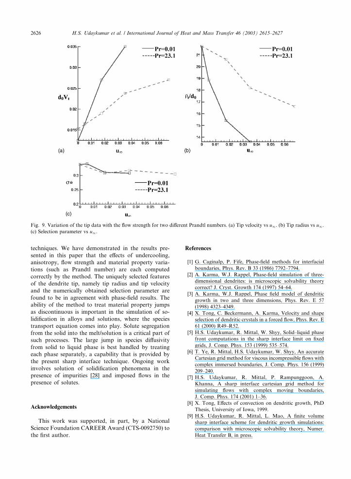
Fig. 9 shows the effects of the Prandtl number and
flow strength on the upstream tip. The tip velocity in
Fig. 9(a) increases with flow strength (Reynolds number)
for both Pr ¼ 23:1 and 0.01. However, the increase forthe lower Prandtl number case is markedly higher than
that for the higher Pr. This large difference indicates thatextrapolation of observations of tip behavior obtained
from model organic materials to metallic materials must
be made with caution. The difference between the two
Prandtl numbers is even more dramatic for the tip ra-
dius. The lower Prandtl number melts will produce
much sharper dendrite tips. As an implication for so-
lidification processing of materials, the dendrite tips in
directions oriented differently with the flow are going to
be much more different in growth rates as well as length
scales for the lower Pr metallic melts than for modelorganic melts. It is worthy of note that the selection
parameter is insensitive to the Prandtl number, at least
for the limited range of parameters explored here. The
selection parameter appears to decrease weakly with the
Reynolds number for both Prandtl numbers. Although
we have not investigated the issue of side-branching in
this paper, once the tip matures noise effects will cause
the tip to become unstable to side-branching [8,23]. The
sharper upstream tip will likely break down first and
the resulting microstructure will reflect the presence of
the side branches, i.e. one would expect finer micro-
structures developed on the upstream side.
In the above, while we have compared our results
quantitatively with the phase-field results we have only
qualitatively compared the behaviors with the linea-
rized solvability theory. The difficulty in quantitatively
Table 1
Comparison of the results from the present sharp-interface calculations with phase-field results of Tong et al.
u1 e Results of V �t q�
t r� Pet Pef
0.031 0.01 Present 0.00925 102.01 0.2077 1.58 0.471
Tong et al. 0.0085 106 0.21 1.64 0.451
0.0675 0.03 Present 0.0238 16.6 0.305 0.56 0.198
Tong et al. 0.0231 17.7 0.28 0.59 0.205
0.0675 0.05 Present 0.031 5.47 2.22 0.185 0.084
Tong et al. 0.029 5.7 2.15 0.193 0.071
Table 2
Tip data obtained for various parameters using the present sharp interface technique
E Pr u1 V �t q�
t r� Pet Pef
0.01 23.1 0.0350 0.0100 92.20 0.0235 0.461 1.614
0.01 23.1 0.0675 0.0115 128.00 0.0106 0.736 4.320
0.02 23.1 0.0675 0.0188 30.77 0.1127 0.288 1.038
0.03 23.1 0.0175 0.0153 20.62 0.3074 0.158 0.180
0.03 23.1 0.0350 0.0190 18.20 0.3178 0.173 0.319
0.03 23.1 0.1400 0.0270 16.53 0.2711 0.194 1.157
0.05 23.1 0.0675 0.0310 5.47 2.2280 0.085 0.185
0.03 0.01 0.0050 0.0165 18.87 0.3404 0.156 0.047
0.03 0.01 0.0175 0.0270 15.43 0.3110 0.208 0.135
0.03 0.01 0.0350 0.0350 13.60 0.3089 0.238 0.238
H.S. Udaykumar et al. / International Journal of Heat and Mass Transfer 46 (2003) 2615–2627 2623

comparing with theory lies in the fact that the theoretical
relationships for tip parameters, given by Eqs. (1) and
(2) are obtained after making several simplifying
assumptions. Chief among these is the assumption of a
translating isothermal paraboloid of revolution. It has
been shown that for large anisotropies the tip deviates
Fig. 7. Tip characteristics vs. flow strength (Reynolds number). For e ¼ 0:03, D ¼ 0:55. (a) The non-dimensional tip velocity vs. u1. (b)Non-dimensional tip radius vs. u1.
Fig. 6. Dendrite solutions with flow. Effect of Prandtl number. (a) Pr ¼ 23:1, u1 ¼ 0:035, e ¼ 0:03 (a1) shows shape evolution and (a2)shows temperature contours at final shape shown. (b) Pr ¼ 0:01, u1 ¼ 0:035, e ¼ 0:03 (b1) shows shapes and (b2) shows the tem-perature contours at final shape shown. (c) Pr ¼ 0:01, u1 ¼ 0:0175, e ¼ 0:03 (c1) shows the shapes and (c2) shows the temperaturecontours at final shape shown.
2624 H.S. Udaykumar et al. / International Journal of Heat and Mass Transfer 46 (2003) 2615–2627

significantly from a paraboloid [8]. This applied both for
the diffusion-driven and forced convection influenced tip
growth cases. In fact, Tong et al. [4] show that if a pa-
rabola is fit to the computed dendrite tip, then the radius
of curvature of such a paraboloid at the tip in combi-
nation with the computed tip velocity gives selection
parameters that are in agreement with the solvability
theory. Thus, while theory is able to provide qualitative
guidance as to the tip behavior and selection mechanism,
quantitative comparisons are only possible when the
assumption of a paraboloidal tip is made.
In Tables 1 and 2 we have tabulated results obtained
for a range of parameters that may prove useful as
benchmarks for the 2D simulations of dendritic growth
with convection as imposed in the present calculations
and Tong et al. [4]. Table 1 compares numerically our
results for different Reynolds numbers and anisotropies
with the available results from Tong et al. The results are
shown to be numerically in excellent agreement with
each other for all the tip characteristics. These results
can therefore be useful as benchmarks. In Table 2 we list
data on the upstream tip for a range of parameters in-
cluding the two Prandtl numbers used. We also list the
value of the selection parameter r� computed for all
cases.
6. Summary
We have developed a numerical method for the
computation of dendritic crystal growth where the so-
lid–liquid interface is treated as a sharp front. Accurate
solution of complicated evolving phase boundaries is
facilitated by maintaining a sharp solid–liquid interface
and the challenge is to develop the sharp-interface
numerics on a mesh that does not conform to the in-
terface shape. The sharp interface nature and the sec-
ond-order spatial and temporal discretization coupled
with a conservative finite volume scheme allows us to
obtain solutions for dendritic crystal growth in good
agreement with theory and with solutions of den-
dritic growth with flow obtained from other numerical
Fig. 8. Tip characteristics (radius, velocity and selection parameter) and their variation with the control and material parameters. (a)
Tip data plotted against the flow strength (equivalently the Reynolds number). (b) Tip Peclet number vs Flow Peclet number for two
values of anisotropy (e ¼ 0:01 and e ¼ 0:03). (c) Tip data plotted against the anisotropy strength for a flow strength of u1 ¼ 0:0675.
H.S. Udaykumar et al. / International Journal of Heat and Mass Transfer 46 (2003) 2615–2627 2625
techniques. We have demonstrated in the results pre-
sented in this paper that the effects of undercooling,
anisotropy, flow strength and material property varia-
tions (such as Prandtl number) are each computed
correctly by the method. The uniquely selected features
of the dendrite tip, namely tip radius and tip velocity
and the numerically obtained selection parameter are
found to be in agreement with phase-field results. The
ability of the method to treat material property jumps
as discontinuous is important in the simulation of so-
lidification in alloys and solutions, where the species
transport equation comes into play. Solute segregation
from the solid into the melt/solution is a critical part of
such processes. The large jump in species diffusivity
from solid to liquid phase is best handled by treating
each phase separately, a capability that is provided by
the present sharp interface technique. Ongoing work
involves solution of solidification phenomena in the
presence of impurities [28] and imposed flows in the
presence of solutes.
Acknowledgements
This work was supported, in part, by a National
Science Foundation CAREER Award (CTS-0092750) to
the first author.
References
[1] G. Caginalp, P. Fife, Phase-field methods for interfacial
boundaries, Phys. Rev. B 33 (1986) 7792–7794.
[2] A. Karma, W.J. Rappel, Phase-field simulation of three-
dimensional dendrites: is microscopic solvability theory
correct? J. Cryst. Growth 174 (1997) 54–64.
[3] A. Karma, W.J. Rappel, Phase field model of dendritic
growth in two and three dimensions, Phys. Rev. E 57
(1998) 4323–4349.
[4] X. Tong, C. Beckermann, A. Karma, Velocity and shape
selection of dendritic crystals in a forced flow, Phys. Rev. E
61 (2000) R49–R52.
[5] H.S. Udaykumar, R. Mittal, W. Shyy, Solid–liquid phase
front computations in the sharp interface limit on fixed
grids, J. Comp. Phys. 153 (1999) 535–574.
[6] T. Ye, R. Mittal, H.S. Udaykumar, W. Shyy, An accurate
Cartesian grid method for viscous incompressible flows with
complex immersed boundaries, J. Comp. Phys. 156 (1999)
209–240.
[7] H.S. Udaykumar, R. Mittal, P. Rampunggoon, A.
Khanna, A sharp interface cartesian grid method for
simulating flows with complex moving boundaries,
J. Comp. Phys. 174 (2001) 1–36.
[8] X. Tong, Effects of convection on dendritic growth, PhD
Thesis, University of Iowa, 1999.
[9] H.S. Udaykumar, R. Mittal, L. Mao, A finite volume
sharp interface scheme for dendritic growth simulations:
comparison with microscopic solvability theory, Numer.
Heat Transfer B, in press.
Fig. 9. Variation of the tip data with the flow strength for two different Prandtl numbers. (a) Tip velocity vs u1. (b) Tip radius vs u1.(c) Selection parameter vs u1.
2626 H.S. Udaykumar et al. / International Journal of Heat and Mass Transfer 46 (2003) 2615–2627

[10] G.B. McFadden, A.A. Wheeler, R.J. Braun, S.R. Coriell,
Phase-field models for anisotropic interfaces, Phys. Rev. E
48 (3) (1993) 2016–2024.
[11] Y.-T. Kim, N. Provatas, N. Goldenfeld, J. Dantzig,
Universal dynamics of phase-field models for dendritic
growth, Phys. Rev. E 59 (3) (1999) R2546–R2549.
[12] T.Y. Hou, Z. Li, S. Osher, H. Zhao, A hybrid method for
moving interface problems with application to the Hele-
Shaw flow, J. Comp. Phys. 134 (2) (1997) 236–247.
[13] Y.-T. Kim, N. Provatas, N. Goldenfeld, J. Dantzig,
Computation of dendritic microstructure using a level-set
method, Phys. Rev E. 62 (2) (2000) 2471–2474.
[14] N. Provatas, N. Goldenfeld, J. Dantzig, Efficient com-
putation of dendritic microstructures using adaptive
mesh refinement, Phys. Rev. Lett. 80 (15) (1998) 3308–
3311.
[15] A. Schmidt, Computation of three-dimensional dendrites
with finite elements, J. Comp. Phys. 125 (1996) 293–
312.
[16] J.M. Sullivan, D.R. Lynch, K. O�Neill, Finite elementsimulations of planar instabilities during solidification of
an undercooled melt, J. Comp. Phys. 69 (1987) 81–111.
[17] D. Juric, G. Tryggvasson, A front tracking method for
dendritic solidification, J. Comp. Phys. 123 (1996) 127–
148.
[18] D.M. Anderson, G.B. McFadden, A.A. Wheeler, Diffuse
interface methods in fluid mechanics, Ann. Rev. Fluid
Mech. 30 (1998) 139–165.
[19] D.A. Kessler, J. Koplik, H. Levine, Pattern selection in
fingered growth phenomena, Adv. Phys. 37 (3) (1988) 255–
339.
[20] G.P. Ivantsov, Temperature field around spherical, cylin-
drical and needle-shaped crystals which grow in super-
cooled melt, Doklady Akademii Nauk SSSR 58 (1947)
567–569.
[21] S.C. Huang, M.E. Glicksman, Fundamentals of dendritic
solidification––I and II, Acta Metall. 29 (1981) 701–715,
717–734.
[22] Ph. Bouissou, P. Pelce, Effect of a forced flow on dendritic
growth, Phys. Rev. A 40 (1989) 509–512.
[23] Ph. Bouissou, B. Perrin, P. Tabeling, Influence of an
external flow on dendritic crystal growth, Phys. Rev. A 40
(1989) 509–512.
[24] Y. Zang, R.L. Street, J.R. Koseff, A non-staggered grid
fractional step method for time-dependent incompress-
ible Navier–Stokes equations in Curvilinear coordinates,
J. Comp. Phys. 114 (1994) 18.
[25] Ph. Bouissou, A. Chiffaudel, B. Perrin, P. Tabeling,
Dendritic side-branching forced by an external flow,
Europhys. Lett. 13 (1990) 89–94.
[26] T.Y. Hou, J.S. Lowengrub, M.J. Shelley, Removing
stiffness from interfacial flows with surface tension,
J. Comp. Phys. 114 (1994) 312.
[27] C. Tu, C.S. Peskin, Stability and instability in the compu-
tation of flows with moving immersed boundaries: a
comparison of three methods, SIAM J. Sci. Stat. Comput.
13 (1992) 1361.
[28] H.S. Udaykumar, L. Mao, Sharp interface simulation of
dendritic solidification of solutions, Int. J. Heat Mass
Transfer 45 (2002) 4793–4808.
[29] M. Plapp, A. Karma, Multiscale finite-difference-diffusion-
Monte-Carlo method for simulating dendritic solidifica-
tion, J. Comp. Phys. 165 (2000) 592–619.
[30] N. Al-Rawahi, G. Tryggvason, Numerical simulation of
denritic solidification with convection: two-dimensional
geometry, J. Comp. Phys. 180 (2002) 471–496.
H.S. Udaykumar et al. / International Journal of Heat and Mass Transfer 46 (2003) 2615–2627 2627