Sharp interface Cartesian grid method II: A technique for simulating droplet interactions with...

Journal of Computational Physics 210 (2005) 32–54

www.elsevier.com/locate/jcp

Sharp interface Cartesian grid method II: A techniquefor simulating droplet interactions with surfaces

of arbitrary shape

H. Liu, S. Krishnan, S. Marella, H.S. Udaykumar *

Department of Mechanical and Industrial Engineering, University of Iowa, Iowa City, IA-52246, United States

Received 1 July 2004; received in revised form 8 March 2005; accepted 17 March 2005

Available online 26 May 2005

Abstract

A fixed-grid, sharp interface method is developed to simulate droplet impact and spreading on surfaces of arbitrary

shape. A finite-difference technique is used to discretize the incompressible Navier–Stokes equations on a Cartesian

grid. To compute flow around embedded solid boundaries, a previously developed sharp interface method for solid

immersed boundaries is used. The ghost fluid method (GFM) is used for fluid–fluid interfaces. The model accounts

for the effects of discontinuities such as density and viscosity jumps and singular sources such as surface tension in both

bubble and droplet simulations. With a level-set representation of the propagating interface, large deformations of the

boundary can be handled easily. The model successfully captures the essential features of interactions between fluid–

fluid and solid–fluid phases during impact and spreading. Moving contact lines are modeled with contact angle hyster-

esis and contact line motion on non-planar surfaces is computed. Experimental observations and other simulation

results are used to validate the calculations.

2005 Elsevier Inc. All rights reserved.

Keywords: Multiphase flow; Sharp interface method; Cartesian grid; Level-sets; Droplet impact

1. Introduction

In Part I [18] an easily implemented three-dimensional sharp interface treatment was developed for solid–

fluid boundaries immersed in flows. The method relied on a framework that meshes well with the sharp-

interface ghost fluid method (GFM) [4,12,16] for fluid–fluid boundaries. In this paper, the sharp-interfacetreatment of the solid–fluid boundaries is combined with the GFM to simulate interactions between

0021-9991/$ - see front matter 2005 Elsevier Inc. All rights reserved.

doi:10.1016/j.jcp.2005.03.032

* Corresponding author. Tel.: +1 319 384 0832; fax: +1 319 335 5669.

E-mail address: [email protected] (H.S. Udaykumar).

mailto:[email protected]

H. Liu et al. / Journal of Computational Physics 210 (2005) 32–54 33

droplets and solid surfaces. The challenge here is to treat all interfaces sharply while allowing for large inter-

face deformations, including fragmentation, and to handle moving contact line dynamics. Treatment of con-

tact line conditions is fairly challenging with the level-set method when compared to say the VOF method [2]

or Lagrangian finite element methods [5]. In the VOF approach the contact angle can be imposed by recon-

structing the partial volume in the fluid–fluid interface cell that lies adjacent to the solid surface such that thereconstructed surface (typically a plane) assumes the specified contact angle with respect to the solid surface

[2]. In the Lagrangian moving mesh approach the mesh node that lies on the solid surface can be moved to

apply the desired angle [5]. For junctions between multiple fluid phases several techniques [26,32] have been

investigated in the level-set framework. For solid–fluid–fluid tri-junctions, Sussman [27] has presented a

technique for applying contact angles. An alternative approach based on a local level-set reconstruction

was outlined by Noble et al. [20]. This second approach has been modified and advanced in the present work;

it was found to be more suitable for situations such as droplet impact, where the contact angle evolves from

the pre-impact to the spreading and equilibrium resting situations. Additionally, the method is designed toenable simulations of droplet spreading on arbitrarily shaped solid surfaces.

2. Methods for simulation of droplet impact

Harlow and Shannon [9] were the first to simulate droplet impact on a solid surface. A ‘‘marker-

and-cell’’ (MAC) finite-difference method was used to solve the NS equations. To simplify the problem,

viscosity and surface tension were neglected so that a physically accurate representation was obtained onlyfor the very initial inertia-dominated stages after impact. Later workers [30] improved the MAC model of

Harlow and Shannon to include surface tension and viscosity effects.

The volume-of-fluid (VOF) method has been used frequently in studying droplet-wall interactions. Tra-

paga and coworkers [28,29] applied a commercial code FLOW-3D, using VOF tracking, to study isother-

mal impingement of liquid droplets in a thermal spray process. Liu et al. [17] used a VOF-based code,

RIPPLE [14] to study the impact of a molten metal droplet and its subsequent solidification. Pasan-

dideh-Fard et al. [22] have shown that the values of contact angle can significantly influence model predic-

tions in combined experimental and numerical studies of droplet impact. The VOF method has also beenapplied to simulate droplet spreading by Renardy et al. [24] for droplets in prior contact with a wall.

Lagrangian finite-element methods were used by Fukai et al. [5–7] to model droplet impact normal to a

flat plate. Like most previous researchers, experimentally measured contact angles were used as inputs to

their previous numerical model. With the inclusion of contact angle dynamics, their model reproduced

experimental data, not only in the spreading phase but also during recoil and oscillation. Baer et al. [1] used

a simple but computationally tractable linear variation between contact line velocity and contact angle in

their 3D simulations. They successfully captured contact angle hysteresis and critical contact angles.

The level-set method was used in combination with a curvilinear grid finite-volume approach by Zhengand Zhang [33] to study droplet spreading and solidification. However, they did not compare their predic-

tions of droplet shapes during impact with experimental or numerical results. Recently the phase field

method, has also been applied to simulations of wetting and spreading of droplets on surfaces [11].

Three-dimensional simulations of droplet impact have only been possible in recent years. Bussmann

et al. [2] demonstrated a three-dimensional, finite difference, fixed-grid Eulerian model using VOF tracking.

Droplet impact and spreading on surfaces of arbitrary shape has also received limited theoretical treatment

in the literature [23]. Droplet impact on an inclined plane and on a step was simulated in [2]. Although their

model for the variation of contact angle with velocity was simplified, the 3D model yielded good predictionsof gross fluid deformation during droplet impact onto an incline and onto an edge.

In the following sections a sharp-interface method is described for the simulation of droplet/ bubble

interactions with arbitrary solid interfaces. The method relies on level-set representations of all interfaces

34 H. Liu et al. / Journal of Computational Physics 210 (2005) 32–54

and provides the capability to follow the dynamics of contact lines. The results are compared with exper-

imental as well as numerical results.

3. The current method

3.1. Equations to be solved

3.1.1. Governing equations

The equations to be solved for viscous incompressible flow are

Continuity equation:

Fig. 1.

along

r ~u ¼ 0; ð1Þ
Momentum equation:
o~uot

þ~u r~u ¼ 1

qrp þ mr2~uþ~g; ð2Þ

where t is time and ~g is the gravitational acceleration. The velocity vector is ~u ¼ hu; v;wi in three-dimen-

sions, pressure is denoted by p and viscosity by m. In the present work, we solve the above equations in

two-dimensional planar as well as axisymmetric situations.

3.1.2. Interface conditions

For a solid–fluid boundary, a no-slip condition is applied everywhere except in the immediate vicinity of

the moving contact line where a slip boundary condition is applied. A Neumann condition is applied for the

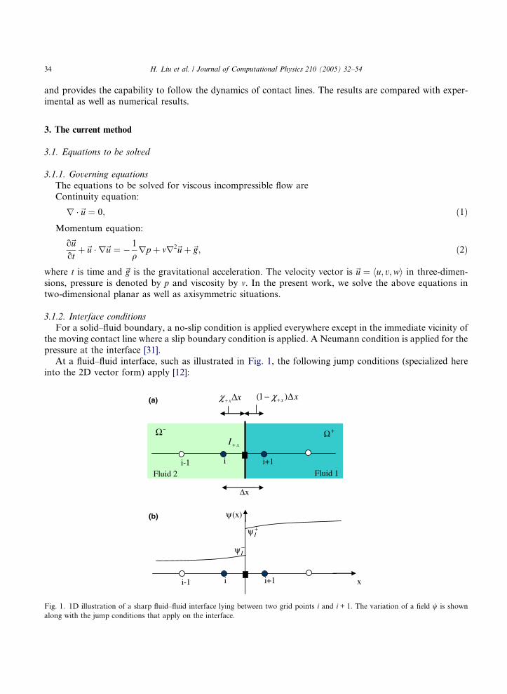
pressure at the interface [31].At a fluid–fluid interface, such as illustrated in Fig. 1, the following jump conditions (specialized here

into the 2D vector form) apply [12]:

xI +

i i+1i-1

∆x

xx∆+χ

i i+1i-1

(x) ψ

ψ

ψ

x

+I

−I

+Ω−Ω

Fluid 1Fluid 2

xx ∆− + )1( χ(a)

(b)

1D illustration of a sharp fluid–fluid interface lying between two grid points i and i + 1. The variation of a field w is shown

with the jump conditions that apply on the interface.


½~u ¼ 0; ð3Þ

½ux ½uy ½vx ½vy

¼ ½l

l

~n~t

T0 0

a 0

~n~t

; ð4Þ

½p 2½lðru ~n;rv ~nÞ ~n ¼ rj; ð5Þ

rpq

¼ lðr2~uÞ

q

. ð6Þ

In the above equations, the square braces indicate jumps in the quantity across the interface, i.e.

½w ¼ wþI w

I , subscript ‘‘I’’ indicates the interfacial value and the normal at the interface points from

the X to X+ side. ~n and~t are the normal and tangent to the interface, respectively. In the above:

a ¼ aaþ

ðaþvþ að1 vÞÞ and l ¼ llþ

ðlþvþ lð1 vÞÞ ; ð7Þ

where

a ¼ ðru ~n;rv ~nÞ ~t þ ðru ~t;rv ~tÞ ~n. ð8Þ
As illustrated in Fig. 1 the level-set information (/1 field for the first immersed interface) can be used [18]
to obtain

v ¼ DxIDx

ffij0 ð/lÞi;jj

jð/lÞiþ1;j ð/lÞi;jj. ð9Þ

3.2. Flow solver

The flow solver is described in detail in [18]. A cell-centered collocated arrangement of the flow vari-

ables is used to discretize the governing equations. A two-step fractional step method [31] is used to ad-

vance the solution in time. A standard level-set evolution equation is used to move the interfaces. For the

grid points away from both fluid–fluid and solid–fluid interfaces, the convection term and pressure gradi-

ent can be computed to second-order accuracy using central differences, which yields a 5-point stencil for

discretization in 2D and results in a symmetric pentadiagonal banded matrix of coefficients. The sharp

interface approach presented in [18] is used to develop discretizations for the interfacial nodes adjacent

to a solid–fluid interface. However, discretization in a sharp fashion for interfacial nodes needs to be per-formed with care when both interfaces (fluid–fluid and solid–fluid) coexist, as can happen during impact

and spreading.

For interfacial points (grid points that satisfy the criterion (/l)i,j(/l)nb 6 0, where ‘‘nb’’ denotes an imme-

diate neighbor along the coordinate directions), the possible situations can be categorized according to the

locations of the interfaces in the computational domain as illustrated in Fig. 2. In the case of a sharp solid–

fluid interface, such as shown in Fig. 2(a) the discretization is given in [18]. When a fluid–fluid interface is

present, the jump conditions make their appearance in the discrete form of the Laplace operator ($ Æ b$w),i.e. in the viscous terms in the momentum equation and in the pressure Poisson equation. For the caseshown in Fig. 2(b) the discretization that includes jump conditions (Eqs. (3)–(6)) is developed according

to the ghost fluid method [12]. For the case in Fig. 2(c) the discretization needs to be carefully handled since

both the solid–fluid interface conditions and the fluid–fluid interface conditions need to be brought into the

discrete operators. For the case in Fig. 2(d) the Fluid 1 layer is below the resolution afforded by the mesh.

IFF

i i+1 i-1 i+2

ISF

i+1i

Fluid

i-1 i+2

LiquidIFF

i+1 i

Solid

i-1 i+2

Fluid 1

IFF ISF

i+1 i

Solid

i-1 i+2

IFF

Fluid 1

Fluid 2 Fluid 2

Fluid1 Fluid 2Solid

(a) (b)

(c) (d)

Fig. 2. Illustration of the different situations that can arise in the fixed grid capture of interacting fluid–fluid and solid–fluid interfaces.

(a) An isolated solid–fluid interface. (b) An isolated fluid–fluid interface. (c) A fluid–fluid interface lying adjacent to a solid–fluid

interface with a grid point lying in the intervening region. (d) A fluid–fluid interface and solid–fluid interface in contact.


In this case the liquid–gas interface is ignored and the discretization then reverts back to that for the solid–

liquid interface in Fig. 2(a).

We will now present a discrete representation of the case in Fig. 2(b) that is drawn from the standard

GFM approach but cast in a form that is compatible with the discrete form for the solid–fluid interfaces

presented in [18]. Then, the discretization procedure for the case in Fig. 2(c) will be presented. For simplic-

ity the discretization is shown for a one-dimensional case (x-direction) only. The discretization for higher

dimensions proceeds in similar fashion independently in each coordinate direction.

3.3. A general form of the discretization for the operators

The jump conditions at the fluid–fluid interfaces manifest themselves primarily in the form (bwx)x.

These arise in the viscous terms in the momentum equation (where b = m) and the pressure Poisson equa-

tion (where b ¼ 1q). Consider the picture in Fig. 2(b). The discretization of the Poisson-type term in the

x-direction proceeds as follows:

ðbwxÞx ¼b ow

ox

iþ1=2j

b owox

i1=2j

Dx. ð10Þ

3.3.1. Case 2 (Fig. 2(b))

If the fluid–fluid interface lies between points (i, j) and (i + 1, j) as shown in Fig. 1(a) and the jump con-

ditions at the interface are [12]:

½w ¼ aIþx ¼ wþIþx

wIþx; ð11Þ

½bwx ¼ bIþx ¼ ðbwxÞþIþx

ðbwxÞIþx. ð12Þ

In discrete form, following the GFM approach [12] the second jump condition can be written as

bþ wiþ1;j wþIþx

ð1 vÞDx

! b w

Iþx wi;j

vDx

¼ bIþx ; ð13Þ


where v is given by Eq. (9). This involves a first-order estimate of the gradients on each side of the interface.

In fact the GFM [12] approach is identical to the IIM [15] if the Taylor expansions in IIM are carried to

first-order only and the second-derivative jumps are ignored.

Using the first jump condition in Eq. (11):

Fig. 3.

Point i

bþ wiþ1;j wIþx

aIþx

ð1 vÞDx

b w

Iþx wi;j

vDx

¼ bIþx . ð14Þ

This gives

wIþx

¼ bþv

ðbþvþbð1 vÞÞwiþ1;jþ

bð1 vÞðbþvþbð1 vÞÞ

wi;jbþv

ðbþvþbð1 vÞÞaIþx

ð1 vÞvDxðbþvþbð1 vÞÞ

bIþx .

ð15Þ
Therefore, using this interfacial value in Eq. (10) one obtains
ðbwxÞx ¼bDx2

ðwiþ1;j wi;jÞ b

Dx2ðwi;j wi1;jÞ

bDx2

aIþx ð1 vÞDx

b

bþ bIþx ; ð16Þ

where

b ¼ bþb

ðbþvþ bð1 vÞÞ. ð17Þ

Similarly, the expression for the case where the interface lies between points (i, j) and (i 1, j) can also beobtained.

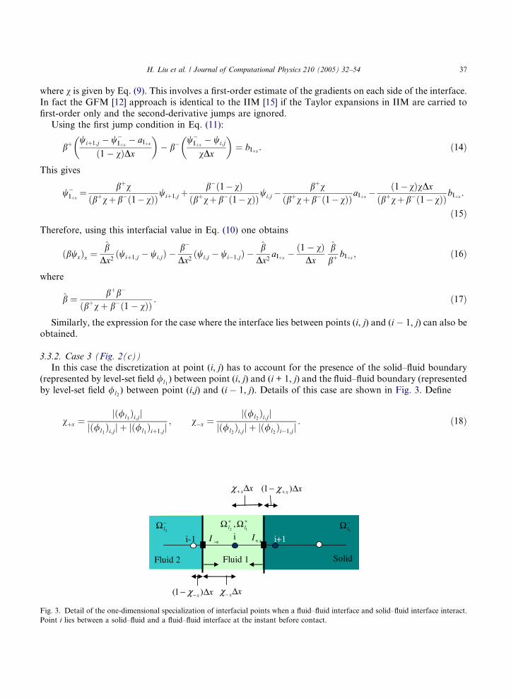
3.3.2. Case 3 (Fig. 2(c))

In this case the discretization at point (i, j) has to account for the presence of the solid–fluid boundary

(represented by level-set field /l1 ) between point (i, j) and (i + 1, j) and the fluid–fluid boundary (represented

by level-set field /l2 ) between point (i,j) and (i 1, j). Details of this case are shown in Fig. 3. Define

vþx ¼jð/l1Þi;jj

jð/l1Þi;jj þ jð/l1Þiþ1;jj; vx ¼

jð/l2Þi;jjjð/l2Þi;jj þ jð/l2Þi1;jj

. ð18Þ

xI −i i+1i-1

xx∆+χ xx ∆− + )1( χ

Fluid 2

xx ∆− − )1( χ xx∆−χ

SolidFluid 1

xI+

−Ω1l

−Ω2l

++ ΩΩ12

, ll

Detail of the one-dimensional specialization of interfacial points when a fluid–fluid interface and solid–fluid interface interact.

lies between a solid–fluid and a fluid–fluid interface at the instant before contact.


A first-order estimate is computed from:

ðbwxÞx ¼bi;j

wþIþx

wi;j

vþxDx

bi;j

wi;jwþIx

vxDx

vþx þ 1

2

Dx

. ð19Þ

Using the jump conditions at the liquid–gas interface:

wþIx

wIx

¼ aIx ; ð20Þ

ðbwxÞþIx

ðbwxÞIx

¼ bIx ¼ bþ ðwi;j wþIxÞ

vxDx b ðw

Ix wi1;jÞ

ð1 vxÞDx. ð21Þ

From the above two expressions one obtains

wþIx

¼ bvx

ðbvx þ bþð1 vxÞÞwi1;j þ

bð1 vxÞðbvx þ bþð1 vxÞÞ

wi;j bvx

ðbvx þ bþð1 vxÞÞaIx

ð1 vxÞvxDxðbvx þ bþð1 vxÞÞ

bIx . ð22Þ

Therefore, substituting in Eq. (19) and simplifying we get

bwxð Þx¼bþ

vþxðvþxþ 12ÞDx2 ðw

þIþx

wi;jÞbx

ðvþxþ 12ÞDx2 ðwi;jwi1;jÞþ

bx

ðvþxþ 12ÞDx2aIx

bx

bDxð1vxÞðvþxþ 1

2ÞDx2bIx ;

ð23Þ
where
bx ¼bbþ

ðbvx þ bþð1 vxÞÞ. ð24Þ

For the situation where the liquid–gas interface lies on the right and the solid–liquid interface lies to theleft a similar expression can be obtained.

3.3.3. The general expression

The situation in Fig. 3 can be considered to be the most general case, encompassing all the cases shown

in Fig. 2(a)–(d). Therefore, based on the expressions obtained for the above two cases and those provided in

[18] for Case 1 (Fig. 2(a)), and considering that Case 4 corresponds to Case 1 (when the unresolved sliver of

the Fluid 1 phase is ignored), a general discrete form for (bwx)x can be obtained. The following expressions

apply where multiple (say Lmax) embedded boundaries are present in the flow:

ðbwxÞx ¼ bþxaþxðwþx wi;jÞ

cxDx2 bxax

ðwi;j wxÞcxDx2

þ bþxaþx

cxDx2þ bxax

cxDx2þ bþxð1 vþxÞbþx

biþ1cxDx2

þ bxð1 vxÞbx

bi1cxDx2; ð25aÞ

where the coefficients bx, a±x and cx are obtained as follows:

ðslÞx ¼ð/lÞi;jð/lÞi1;j

jð/lÞi;jð/lÞi1;jj

( ); sx ¼ min

l¼1;Lmax

ðslÞx

; ð25bÞ


vx ¼ minl¼1;Lmax

jmaxððslÞx; 0Þj þjð/lÞi;jj

jð/lÞi;jj þ jð/lÞi1;jjjminððslÞx; 0Þj

( ); ð25cÞ

dx ¼1 if solid–fluid interface between ði; jÞ and ði 1; jÞ;0 otherwise;

ð25dÞ

wx ¼ dxwIxþ ð1 dxÞwi1;j; ð25eÞ

ax ¼ dx1

vxþ ð1 dxÞ; ð25fÞ

bx ¼bi;jbi1;j

bi;jvx þ bi1;jð1 vxÞ; ð25gÞ

cx ¼ dþxvþx

2þ dx

vx

2þ ð1 dþxÞ

1

2þ 1

2vxdxjminðsþx; 0Þj

þ ð1 dxÞ

1

2þ 1

2vþxdþxjminðsx; 0Þj

ð25hÞ

ax ¼ð/l1Þi;jjð/l1Þi;jj

aIx jminðsx; 0Þjð1 dxÞ; ð25iÞ

bx ¼ ð/l2Þi;jjð/l2Þi;jj

bIx jminðsx; 0Þjð1 dxÞ. ð25jÞ

The advantage of casting the equations in the above form is that implementation in a computer code is

straightforward. Note that Eqs. (25) reduce, in the appropriate cases, to the discrete form for a solid–fluidinterface obtained in Marella et al. (2004), to Eq. (16) for a fluid–fluid interface, and to standard central

differences in the absence of interfaces. The above coefficient assembly also applies to any point in the do-

main, including points that lie away from the interface and interface adjacent points that conform to any of

the cases shown in Fig. 2. Thus, a sharp-interface calculation that handles solid–fluid immersed bound-

aries, fluid–fluid immersed boundaries and their interactions can be easily programmed by a few lines of

code that modify a simple uniform Cartesian grid flow solver. The discretization of the components of

the Laplace operator involving derivatives in the y- and z-directions is performed with procedures identical

to that presented above for the x-derivatives. The above form unifies the treatment of the sharp interfacemethod presented in [18] with the ghost-fluid method [12], and is a first-order implementation of the im-

mersed interface method [15]. The treatment of the convection term proceeds in a fashion identical to that

described in [18].

4. Velocity correction

Once the intermediate velocity and pressure fields have been obtained as described above, the velocity

correction step is performed to update to a divergence-free velocity field. For grid points that lie away from

the interface this is straightforward. For points that lie next to the immersed boundary the corrections are

to be performed based on the different situations that may arise at such points, as illustrated in Fig. 2. The

pressure gradients required to correct the cell center and cell face velocities have to be evaluated in a man-ner consistent with the evaluation performed for obtaining the gradients while discretizing the Laplace


operator in the PPE. For the case shown in Fig. 2(a) the correction procedure has been provided in [18]. For

the particular case illustrated in Figs. 2(b) the corrections are effected as follows:

unþ1i;j ¼ ui;j

Dtqi;jDxð12 þ vþxÞ

ðpIþx pi1=2;jÞ; ð26Þ

unþ1iþ1=2;j ¼ uiþ1=2;j

Dtqiþ1=2;jDxvþx

ðpIþx pi;jÞ. ð27Þ

For the case in Fig. 2(c) the corrections are obtained from:

unþ1i;j ¼ ui;j

Dtqi;jDxðvx þ vþxÞ

ðpþIþx pþIx

Þ; ð28Þ

unþ1iþ1=2;j ¼ uiþ1=2;j

Dtqiþ1=2;jDxvþx

ðpþIþx pi;jÞ; ð29Þ

unþ1i1=2;j ¼ ui1=2;j

Dtqi1=2;jDxvx

ðpi;j pþIxÞ. ð30Þ

In the above equations, the interface pressure in case of fluid–fluid interfaces is obtained by applying the

jump conditions for pressure listed in Eqs. (5) and (6). In the case of solid–fluid interfaces, the pressure is

obtained by as described in [18].

A compact way of writing the corrections for all the situations is

unþ1i;j ¼ ui;j

Dtqi;j

axðpþx pxÞDx

; ð31aÞ

where

pþx ¼ piþ1=2;jjmaxðsþx; 0Þj þ pIþxjminðsþx; 0Þj; ð31bÞ

px ¼ pi1=2;jjmaxðsx; 0Þj þ pIxjminðsx; 0Þj; ð31cÞ

ax ¼1

ðvþx þ vxÞ; ð31dÞ

ðslÞx ¼ð/lÞi;jð/lÞiþ1;j

jð/lÞi;jð/lÞiþ1;jj

( ); sx ¼ min

l¼1;Lmax

fðslÞxg; ð31eÞ

vx ¼1þ jminðsx; 0Þjð Þ

2min

l¼1;Lmax

jmaxððslÞx; 0Þj þjð/lÞi;jj

jð/lÞi;jj þ jð/lÞi1;jjjminððslÞx; 0Þj

( ). ð31fÞ

Note that cell face velocities are corrected independently:

~unþ1iþ1=2;j ¼~uniþ1=2;j Dt

opnþ1

ox

iþ1=2;j

. ð32Þ

The pressure gradient at the cell face is obtained based on straightforward central differences. The dis-

crete correction expressions are similar to those given above.


5. Modeling the moving contact line

The precise relationship between contact line velocity and contact angle is poorly understood and most

researchers have simplified this problem by employing experimentally measured contact angles as input

boundary conditions for their numerical models. Pasandideh-Fard et al. [21] used the measured contact an-gle from photographs obtained from experiments as inputs to their numerical model. Fukai et al. [5] em-

ployed a similar approach in their study of wetting effects. Bussmann et al. [2] developed a model to

evaluate contact angles as a function of contact line velocity. This model requires two inputs as well, the

advancing and receding contact angles. Baer et al. [1] used a computationally tractable but simplified linear

dependence of the contact angle on contact line velocity in their 3D finite-element moving mesh simula-

tions. The model successfully accounted for the observed features of droplet spreading in 3D such as con-

tact angle hysteresis and static contact angles. However, to ensure computational robustness for modeling

wetting effects, a huc correlation is required to be applicable simultaneously to advancing and recedingcontact lines and over a large range of flow situations and geometry. Such a general relation is not available

in the literature. In the following simulations, for modeling the contact angle depicted in Fig. 4(a), hrecedingand hadvancing are assumed constant, as illustrated in Fig. 4(b). This is not a methodological limitation how-

ever and more sophisticated models for contact angle behavior, once established, can be easily included

within the current framework.

Numerical modeling of fluid behavior in the vicinity of a moving contact line is complicated because the

no-slip boundary condition at the solid–liquid interface leads to a force singularity at the contact line [10].

The problem can be resolved by replacing the no-slip boundary condition with a slip model [3]. Althoughthis alleviates mathematical difficulties, there is no experimental evidence to determine which of the several

available slip models is the most appropriate to use or whether physically such slip even occurs. In the pres-

ent study, we simply apply the Navier slip boundary condition in the vicinity of the contact line. That is, we

Fig. 4. (a) Axisymmetric droplet schematic and contact angle specification. (b) Illustration of model for the velocity dependent contact

angle. (c) Illustration of implementation of slip boundary conditions for contact points.


allow the contact line to slip in a direction tangent to the substrate and thus alleviate the local singularity.

In general form, the Navier slip boundary condition is:~s ¼ llsutwall , where~s is the tangential component of

the surface traction vector, ls is a slip length and the subscript twall indicates the value at the wall tangential

to it. This is estimated in the current paper for an arbitrarily oriented solid surface from: l outon ¼

llsutwall ,

where n denotes the length increment in the normal direction to the surface and subscript t indicates thetangential wall component. By discretizing the normal gradient using a two-point discrete form and obtain-

ing the value of velocity at the end of a normal projected [18] into the fluid from the contact point the value

of utwall is obtained from the above slip condition. The slip length ls was chosen to be Dx, the grid spacing

[24]. The slip boundary condition is only applied to the fluid points which are in the immediate vicinity of

the contact line. Fig. 4(c) illustrates the procedure for imposition of the slip boundary condition. First, a

‘‘contact point’’ is identified, which is the grid point in the spreading fluid that is immediately adjacent

to the liquid–gas–solid tri-junction. Two other grid points that are the closest points to the identified con-

tact point lying in the liquid and gas phases respectively are also identified. These three grid points in thefluid are given the Navier slip boundary condition on the wall, thus allowing the movement of the contact

line. In the direction normal to the surface, the usual no-penetration boundary condition is employed at all

solid-adjacent points.

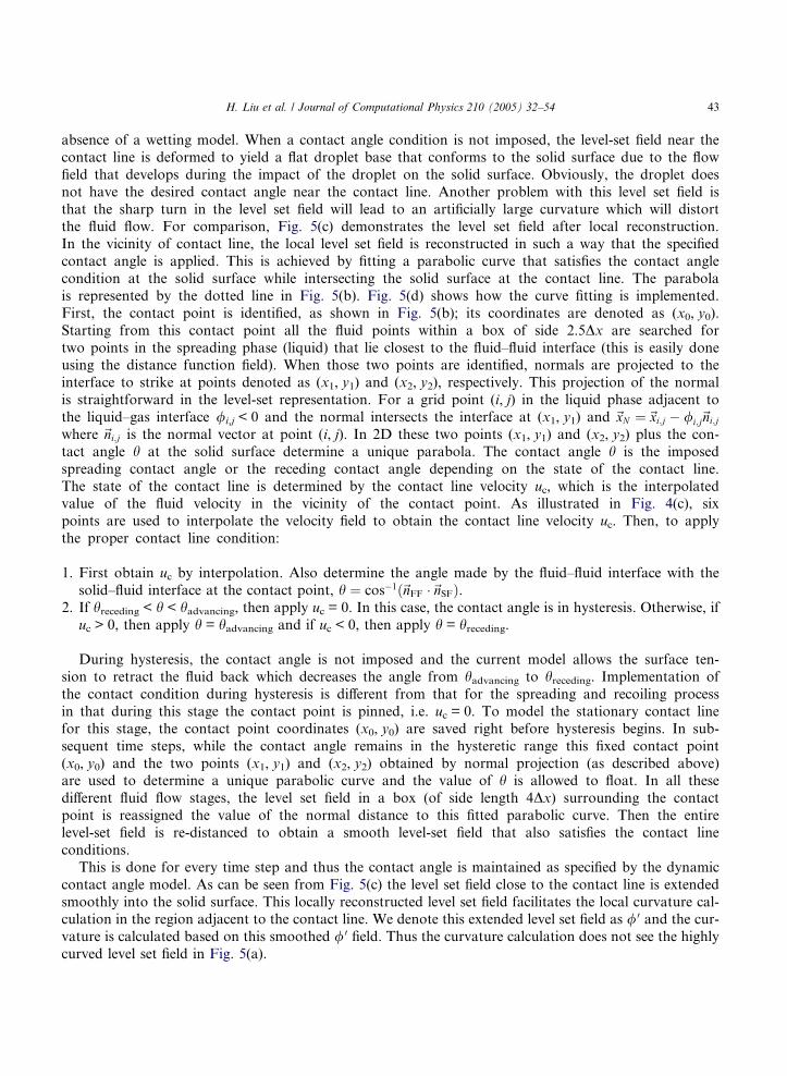
6. Local level set reconstruction method for setting the contact angle

Fig. 5 illustrates the procedure employed to enforce the contact angle boundary condition on thesolid surface. Fig. 5(a) shows the level set contour for a drop impacting on a solid surface in the

Fig. 5. Illustration of level set reconstruction and parabola fitting with a desired contact angle (92). (a) Original level-set field. (b)

Local parabola fitting. (c) Level-set field after reconstruction. (d) Illustration of parabolic curve fitting in level set field.


absence of a wetting model. When a contact angle condition is not imposed, the level-set field near the

contact line is deformed to yield a flat droplet base that conforms to the solid surface due to the flow

field that develops during the impact of the droplet on the solid surface. Obviously, the droplet does

not have the desired contact angle near the contact line. Another problem with this level set field is

that the sharp turn in the level set field will lead to an artificially large curvature which will distortthe fluid flow. For comparison, Fig. 5(c) demonstrates the level set field after local reconstruction.

In the vicinity of contact line, the local level set field is reconstructed in such a way that the specified

contact angle is applied. This is achieved by fitting a parabolic curve that satisfies the contact angle

condition at the solid surface while intersecting the solid surface at the contact line. The parabola

is represented by the dotted line in Fig. 5(b). Fig. 5(d) shows how the curve fitting is implemented.

First, the contact point is identified, as shown in Fig. 5(b); its coordinates are denoted as (x0, y0).

Starting from this contact point all the fluid points within a box of side 2.5Dx are searched for

two points in the spreading phase (liquid) that lie closest to the fluid–fluid interface (this is easily doneusing the distance function field). When those two points are identified, normals are projected to the

interface to strike at points denoted as (x1, y1) and (x2, y2), respectively. This projection of the normal

is straightforward in the level-set representation. For a grid point (i, j) in the liquid phase adjacent to

the liquid–gas interface /i,j < 0 and the normal intersects the interface at (x1, y1) and ~xN ¼~xi;j /i;j~ni;jwhere ~ni;j is the normal vector at point (i, j). In 2D these two points (x1, y1) and (x2, y2) plus the con-

tact angle h at the solid surface determine a unique parabola. The contact angle h is the imposed

spreading contact angle or the receding contact angle depending on the state of the contact line.

The state of the contact line is determined by the contact line velocity uc, which is the interpolatedvalue of the fluid velocity in the vicinity of the contact point. As illustrated in Fig. 4(c), six

points are used to interpolate the velocity field to obtain the contact line velocity uc. Then, to apply

the proper contact line condition:

1. First obtain uc by interpolation. Also determine the angle made by the fluid–fluid interface with the

solid–fluid interface at the contact point, h ¼ cos1ð~nFF ~nSFÞ.2. If hreceding < h < hadvancing, then apply uc = 0. In this case, the contact angle is in hysteresis. Otherwise, if

uc > 0, then apply h = hadvancing and if uc < 0, then apply h = hreceding.

During hysteresis, the contact angle is not imposed and the current model allows the surface ten-

sion to retract the fluid back which decreases the angle from hadvancing to hreceding. Implementation of

the contact condition during hysteresis is different from that for the spreading and recoiling process

in that during this stage the contact point is pinned, i.e. uc = 0. To model the stationary contact line

for this stage, the contact point coordinates (x0, y0) are saved right before hysteresis begins. In sub-

sequent time steps, while the contact angle remains in the hysteretic range this fixed contact point

(x0, y0) and the two points (x1, y1) and (x2, y2) obtained by normal projection (as described above)are used to determine a unique parabolic curve and the value of h is allowed to float. In all these

different fluid flow stages, the level set field in a box (of side length 4Dx) surrounding the contact

point is reassigned the value of the normal distance to this fitted parabolic curve. Then the entire

level-set field is re-distanced to obtain a smooth level-set field that also satisfies the contact line

conditions.

This is done for every time step and thus the contact angle is maintained as specified by the dynamic

contact angle model. As can be seen from Fig. 5(c) the level set field close to the contact line is extended

smoothly into the solid surface. This locally reconstructed level set field facilitates the local curvature cal-culation in the region adjacent to the contact line. We denote this extended level set field as / 0 and the cur-

vature is calculated based on this smoothed / 0 field. Thus the curvature calculation does not see the highly

curved level set field in Fig. 5(a).


7. Results

7.1. Droplet impact normal to a flat surface in the absence of a wetting model

Fig. 6 shows the impact, spreading and recoil behavior of a droplet impinging on a flat surface forthe non-dimensional parameters Re = 120, We = 80, Fr = 105. To validate the calculations, the thickness

(at the symmetry axis) of the spreading drop is plotted against time for different Reynolds numbers in

Fig. 6. Sequence of droplet shapes for normal impact on a solid plane surface impacting with parameters Re = 120, We = 80, Fr = 105.

Fig. 7. (a) Effects of Reynolds number on the thickness of the droplet at the center of the axis of symmetry. (b) Spreading radius as a

function of dimensionless time.


Fig. 7. The Weber number is held constant for these cases (We = 80). In Fig. 7(a), the results are compared

with the experimental measurements carried out by Savic and Boult [25] using a high speed camera. The

experiments were conducted with water droplets 4.8 mm in diameter, falling from a height of 1.83 m cor-

responding to Re = 2.9 · 104. It is seen that very good agreement for the early stage of spreading is obtained

with the present calculation. For the duration immediately after impact, the droplet motion is inertia dom-inated and is independent of viscous and capillary effects. This similarity in spreading lasts up to t* = 2,

demonstrating high rates of change in thickness independent of Reynolds number. Based on their analysis,

Trapaga and Szekely [29] gave a linear relation between the impact velocity and dimensionless time for this

very early stage of impact as dhdt ¼ coV o with co ranging from 0.7 to 0.84. Based on the predictions of our

numerical model, we obtain dhdt 0.813, which falls within the range given by Trapaga et al.

An important characteristic quantity in thermal spraying of metal droplets [7,8,19] is the final thickness

at the center of the solidified splat. In an experimental study, [34] measured values of splat thickness for

plasma-sprayed alumina powder with diameters ranging from 20 to 100 lm. It was found that the splatthickness is in the range of 2–4 lm. Trapaga and Szekely [29] suggest that the final thickness at the center

is only a small fraction (5%) of the initial droplet diameter. The final thickness obtained in the current sim-

ulations range from 4% to 15%. Fukai et al. [6] found that their calculated final splat thickness is around

10% of the pre-impact droplet radius. While in our predictions, for Reynolds number of 1200 and 6000, the

predicted results are in very good agreement with above reference values (@5%), the result (@14%) for small

Reynolds number (Re = 120) is slightly above the suggested value of 10% by Fukai et al. [6]. Another char-

acteristic trend observed is that the final splat thickness is dependent on Reynolds numbers, with larger

Reynolds numbers tending to have smaller maximum thickness as expected. This is clearly demonstratedin Fig. 7(b) and is consistent with the observations of Fukai et al. [5] and Trapaga and Szekely [29]. This

phenomenon is also consistent with the notion that higher Reynolds numbers should correspond to larger

maximum spreading radii, as shown in Fig. 7(b).

7.2. Droplet impact on arbitrarily shaped solid surfaces

Simulations of impact of droplets on solid surfaces of arbitrary shape are relatively sparse in the liter-

ature. Of the available simulations [2,23] none are sharp-interface models for the fluid–fluid interfaceand the solid–fluid interface is typically treated in a simplistic manner by using a volume-fraction solid

Fig. 8. Shapes of a droplet impacting on a cylinder (Re = 10, We = 333). The formation of a filament on each side is seen along with

the detachment of a pendant drop and formation of a secondary pendant drop after retraction of the remaining filament.


approach or a stair-step geometry aligned with the Cartesian mesh. The methodology developed in this pa-

per allows for the calculation of impact on arbitrarily shaped solid objects, without these limitations of pre-

vious methods. By using the general form of the discretization scheme shown in Eq. (25) independently

along each coordinate direction, the treatment of impact on curved surfaces is no different from that on

a plane surface. Here we demonstrate the capability of the method to solve the impact problem withoutinvolving the issue of contact line dynamics. Results with wetting effects are presented in a subsequent

section.

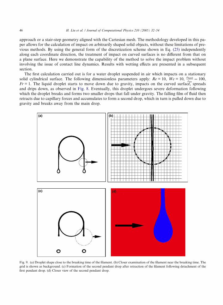
The first calculation carried out is for a water droplet suspended in air which impacts on a stationary

solid cylindrical surface. The following dimensionless parameters apply: Re = 10, We = 10,qliquidqgas

¼ 100,

Fr = 1. The liquid droplet starts to move down due to gravity, impacts on the curved surface, spreads

and drips down, as observed in Fig. 8. Eventually, this droplet undergoes severe deformation following

which the droplet breaks and forms two smaller drops that fall under gravity. The falling film of fluid then

retracts due to capillary forces and accumulates to form a second drop, which in turn is pulled down due togravity and breaks away from the main drop.

Fig. 9. (a) Droplet shape close to the breaking time of the filament. (b) Closer examination of the filament near the breaking time. The

grid is shown as background. (c) Formation of the second pendant drop after retraction of the filament following detachment of the

first pendant drop. (d) Closer view of the second pendant drop.


To demonstrate the ability of the method to capture the interface sharply, it is useful to amplify further

the features observed in Fig. 8. As illustrated in Fig. 9(a), two very thin filaments are formed on the two

sides of the spreading droplet which eventually result in drops. Amplifying this thin filament, as shown

in Fig. 9(b), it is observed that the entire filament lies within two mesh widths. The detail of the secondary

drop formed after the film of fluid retracts following detachment of the first breakaway satellite drop is alsoshown in Fig. 9(c) and (d). The present sharp interface method can handle these rather fine structures ro-

bustly and can also compute through topological changes without difficulty. Note that the calculations were

performed in a two-dimensional system without imposing symmetry, i.e. the entire cylinder and drop was

computed. The method preserves very well the symmetry of the evolution of the fluid–fluid boundary.

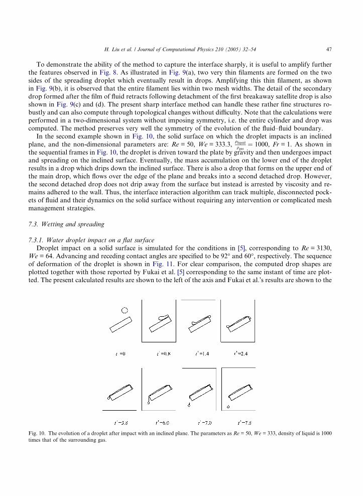
In the second example shown in Fig. 10, the solid surface on which the droplet impacts is an inclined

plane, and the non-dimensional parameters are: Re = 50, We = 333.3,qliquidqgas

¼ 1000, Fr = 1. As shown in

the sequential frames in Fig. 10, the droplet is driven toward the plate by gravity and then undergoes impact

and spreading on the inclined surface. Eventually, the mass accumulation on the lower end of the dropletresults in a drop which drips down the inclined surface. There is also a drop that forms on the upper end of

the main drop, which flows over the edge of the plane and breaks into a second detached drop. However,

the second detached drop does not drip away from the surface but instead is arrested by viscosity and re-

mains adhered to the wall. Thus, the interface interaction algorithm can track multiple, disconnected pock-

ets of fluid and their dynamics on the solid surface without requiring any intervention or complicated mesh

management strategies.

7.3. Wetting and spreading

7.3.1. Water droplet impact on a flat surface

Droplet impact on a solid surface is simulated for the conditions in [5], corresponding to Re = 3130,

We = 64. Advancing and receding contact angles are specified to be 92 and 60, respectively. The sequenceof deformation of the droplet is shown in Fig. 11. For clear comparison, the computed drop shapes are

plotted together with those reported by Fukai et al. [5] corresponding to the same instant of time are plot-

ted. The present calculated results are shown to the left of the axis and Fukai et al.s results are shown to the

Fig. 10. The evolution of a droplet after impact with an inclined plane. The parameters as Re = 50, We = 333, density of liquid is 1000

times that of the surrounding gas.

Fig. 11. Calculated droplet spreading shapes compared with numerical results from Fukai et al. (1996) for droplet impact with

Re = 3010, We = 57, hadvancing = 92, hreceding = 60, hstatic = 75.


right. It is observed that a thin film is formed around the droplet right after the impact. Consistent with

Fukais prediction, the spreading process ends at t* = 7.5. During this spreading process, the contact angle

(see Fig. 11(c)) is maintained at the advancing value of 92 as specified by the model. Contact angle hys-teresis takes place approximately from t* = 5.0 to t* = 7.0. After t* = 7.5, the recoil process begins and

the fluid recedes from the maximum wetted radius at the specified receding contact angle. A bulk upward


motion near the axis occurs after t* = 28 and oscillation of the droplet ensues after this time. Equilibrium is

achieved after a few oscillations. The equilibrium shape of the drop is characterized by a typical sessile

spherical cap drop shape with an equilibrium angle of 75. This angle has a value between the advancing

and receding contact angle.

The above simulation successfully captures all the essential features of droplet impact. From Fig. 11, itcan be seen that very close match is obtained with the results from [5] in terms of drop shapes and timing of

all the characteristic processes. However, some differences in the predictions of the maximum spreading ra-

dius and droplet thickness are observed. The maximum spreading radius reported by Fukai et al. in this

case is 3.6; the current predicted result is 3.45. This difference is also reflected as a discrepancy in the max-

imum drop thicknesses. The current model obtains 2.35 while Fukai et al. reported a value of 2.7. These

differences can be better seen in Fig. 12, in which the current computed spreading radius (Fig. 12(a)) as well

as the droplet thickness (Fig. 12(b)) are compared with the experimental results provided by Fukai et al.

However, the time for the droplet to reach maximum spreading from our calculation is 4.2, which is inexcellent agreement with that reported by Fukai et al. The match in time can also be seen by comparing

subsequent hysteresis and spreading and recoil processes.

Fig. 12. Quantitative results for Re = 3010, We = 57, hadvancing = 92, hreceding = 60, hstatic = 75. (a) Calculated droplet spreading

radius compared with experimental results. (b) Calculated droplet thickness compared with experimental results. (c) Contact angle for

water droplet.


Fig. 12(c) depicts the contact angle as a function of time. As observed from this figure, if the droplet is

spreading, a pre-specified constant advancing contact angle (92) is imposed. If the droplet undergoes

recoiling, a specified constant receding contact angle (60) is imposed. During hysteresis, no fixed contact

angle is imposed but the contact angle is free to be adjusted by surface tension while the contact line

remains motionless.

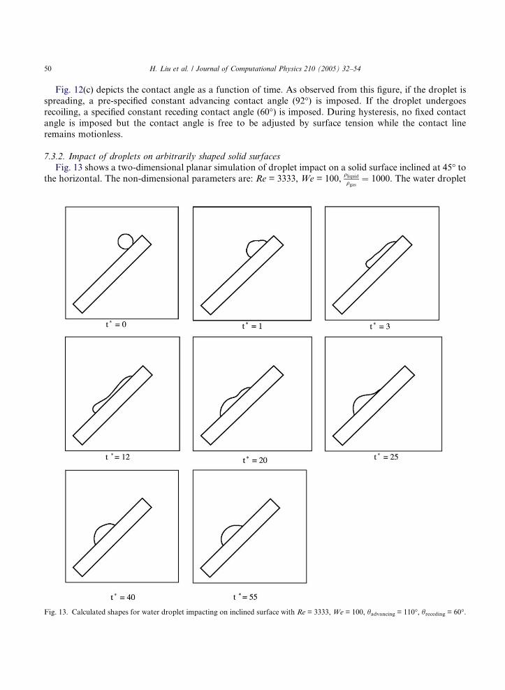
7.3.2. Impact of droplets on arbitrarily shaped solid surfaces

Fig. 13 shows a two-dimensional planar simulation of droplet impact on a solid surface inclined at 45 tothe horizontal. The non-dimensional parameters are: Re = 3333, We = 100,

qliquidqgas

¼ 1000. The water droplet

Fig. 13. Calculated shapes for water droplet impacting on inclined surface with Re = 3333, We = 100, hadvancing = 110, hreceding = 60.


is given an initial dimensionless impact velocity of 1. Apart from the fact that the solid geometry immersed

in the Cartesian mesh is not coincident with the coordinate directions, this case also differs from the

previous cases in that there are two contact lines in this impact scenario. These two contact lines move

with different velocities and thus are represented by different contact angles. One can clearly identify two

Fig. 14. Calculated shapes for water droplet impacting on curved surface with Re = 3333, We = 50, hadvancing = 110, hreceding = 60.


distinctive contact angles when the droplet is sliding down the curved surface, the one to the left is the

advancing (110) and on the right is the receding (60) contact angle. The droplet undergoes spreading, hys-teresis, recoiling, as well as subsequent oscillations as it slides down the plane. It eventually reaches a static

shape represented by two distinctive static contact angles. The upper contact line has an angle 69 and the

lower contact angle is 72. An experimental study of droplet impact on an inclined surface can be found inKang et al. (2000) [13]. Their study included heat transfer and its effects on the droplet spreading. The drop-

let shapes obtained in the above simulation are qualitatively similar to those in the experiments for similar

parameter values. Bussmann et al. [2] numerically modeled three-dimensional droplet impact on an inclined

surface using a VOF representation for the fluid and a volume-fraction approach for the solid. Droplet

shapes and spreading behavior similar to those seen in the present 2D simulations were observed, both

in terms of the droplet shapes as well as the final displacement and resting shape.

To demonstrate that droplet impact with wetting effects can be simulated on an arbitrary-shaped sur-

face, impact onto a shape like a sinusoid shaped solid surface is shown in Fig. 14. The key parametersare: Re = 3333, We = 50,

qliquidqgas

¼ 1000, hadvancing = 110, hreceding = 60. The sequence of deformation of

the droplet is depicted in the figure. The droplet is seen to flow down the surface to the trough, with

the specified receding and advancing contact angles. It overshoots the trough due to inertia but finally

settles to equilibrium in the trough with the resting contact angle values of 88.3 and 86.5 at the two

contact lines.

8. Summary

A sharp-interface method is presented in this paper for the simulation of fluid–fluid interfaces interacting

with solid–fluid interfaces. The specific problem of impact of droplets with surfaces of arbitrary shape is

chosen to demonstrate the technique. The framework of the method rests on a level-set representation

of all interfaces. This allows for easy implementation of a finite-difference scheme to discretize the govern-

ing equations in the presence of interfaces in such a way that explicit knowledge of the interface location is

not necessary. The implicit embedded interface derived from the level-set field suffices to provide a sharp

description of the interface and to apply the necessary boundary conditions and jump conditions on theinterfaces. The discretization scheme unifies a sharp-interface solid–fluid interface treatment presented in

[18] with the ghost-fluid method. One crucial aspect of multiphase interactions is the wetting of the solid

surface by the fluid and the dynamics of the three-phase contact line. The model to include this dynamics

on an arbitrarily shaped solid has been advanced in this paper within the framework of a sharp-interface

approach.

The method has been used to study the impact of droplets in several scenarios and a range of parameters

has been covered. The results are shown to match other numerical and experimental results well in the

range of parameters explored. This includes problems where the contact line dynamics is important. Bench-mark results for the impact and spreading of droplets on arbitrary surfaces are lacking. In such cases, the

method is shown to provide qualitatively correct solutions. Study of the three-dimensional droplet-surface

interaction problem is now in progress.

Acknowledgments

This work was performed with support from the Computational Mechanics Branch, AFRL-MNAC,Eglin, FL (Project manager Mr. Joel Stewart) and AFOSR Computational Mathematics Division (Pro-

gram manager Dr. Fariba Fahroo).


References

[1] T.A. Baer, R.A. Cairncross, P.R. Schunk, R.R. Rao, P.A. Sackinger, A finite element method for free surface flows of

incompressible fluids in three dimensions. Part II: Dynamic wetting lines, International Journal for Numerical Methods in Fluids

33 (3) (2000) 405.

[2] M. Bussmann, J. Mostaghimi, S. Chandra, On a three-dimensional volume tracking model of droplet impact, Physics of Fluids 11

(6) (1999) 1406–1417.

[3] E.B. Dussan, E. Rame, S. Garoff, On identifying the appropriate boundary-conditions at a moving contact line – an experimental

investigation, Journal of Fluid Mechanics 230 (1991) 97–116.

[4] R. Fedkiw, X.-D. Liu, The ghost fluid method for viscous flows, in: M. Hafez, J.-J. Chattot (Eds.), Innovative Methods for

Numerical Solutions of Partial Differential Equations, World Scientific Publishing, New Jersey, 2002, pp. 111–143.

[5] J. Fukai, Y. Shiiba, T. Yamamoto, O. Miyatake, D. Poulikakos, C.M. Megaridis, Z. Zhao, Wetting effects on the spreading of a

liquid droplet colliding with a flat surface – experiment and modeling, Physics of Fluids 7 (2) (1995) 236–247.

[6] J. Fukai, Z. Zhao, D. Poulikakos, C.M. Megaridis, O. Miyatake, Modeling of the deformation of a liquid droplet impinging

upon a flat surface, Physics of Fluids A – Fluid Dynamics 5 (11) (1993) 2588–2599.

[7] R. Ghafouri-Azar, S. Shakeri, S. Chandra, J. Mostaghimi, Interactions between molten metal droplets impinging on a solid

surface, International Journal of Heat and Mass Transfer 46 (8) (2003) 1395–1407.

[8] E. Gutierrezmiravete, E.J. Lavernia, G.M. Trapaga, J. Szekely, N.J. Grant, A mathematical-model of the spray deposition

process, Metallurgical Transactions A – Physical Metallurgy and Materials Science 20 (1) (1989) 71–85.

[9] F.H. Harlow, J.P. Shannon, The splash of liquid droplet, Journal of Applied Physics 38 (1967) 3885.

[10] L.M. Hocking, Rival contact-angle models and the spreading of drops, Journal of Fluid Mechanics 239 (1992) 671–681.

[11] D. Jacqmin, An energy approach to the continuum surface method, in: 34th Aerospace Science Meeting, No. AIAA-96-0858,

1996.

[12] M. Kang, R.P. Fedkiw, A boundary condition capturing method for multiphase incompressible flow, Journal of Scientific

Computing 15 (2002) 323–360.

[13] B.S. Kang, D.H. Lee, On the dynamic behavior of a liquid droplet impacting upon an inclined heated surface, Experiments in

Fluids 29 (4) (2000) 380–387.

[14] D.B. Kothe, R.C. Mjolsness, M.D. Torrey, Ripple: A computer program for incompressible flows with free surfaces, Technical

Report LA-12007-MS, 1991.

[15] Z.L. Li, M.C. Lai, The immersed interface method for the Navier–Stokes equations with singular forces, Journal of

Computational Physics 171 (2) (2001) 822–842.

[16] X.D. Liu, R.P. Fedkiw, M.J. Kang, A boundary condition capturing method for Poissons equation on irregular domains,

Journal of Computational Physics 160 (1) (2000) 151–178.

[17] Liu, Huimin, Enrique J. Lavernia, Roger H. Rangel, Numerical simulation of substrate impact and freezing of droplets in

plasma spray processes, Journal of Physics D: Applied Physics 26 (11) (1993) 1900–1908.

[18] S. Marella, S. Krishnan, H. Liu, H.S. Udaykumar, Sharp interface Cartesian grid method I: an easily implemented technique for

3D moving boundary computations, Journal of Computational Physics (accepted).

[19] J. Mostaghimi, M. Pasandideh-Fard, S. Chandra, Dynamics of splat formation in plasma spray coating process, Plasma

Chemistry and Plasma Processing 22 (1) (2002) 59–84.

[20] D.R. Noble, T.A. Baer, R.R. Rao, Contact angle specification in level-set simulations, Sandia National Laboratories Internal

Report, 1994; Obtained by private communication with D.R. Noble.

[21] M. Pasandideh-Fard, Y.M. Qiao, S. Chandra, J. Mostaghimi, Effect of surface tension and contact angle on the spreading of a

droplet impacting on a substrate, American Society of Mechanical Engineers, Fluids Engineering Division (Publication) FED,

Experimental and Numerical Flow Visualization 218 (1995) 53–61.

[22] M. Pasandideh-Fard, R. Bhola, S. Chandra, J. Mostaghimi, Deposition of till droplets on a steel plate: simulations and

experiments, International Journal of Heat and Mass Transfer 41 (19) (1998) 2929–2945.

[23] M. Pasandideh-Fard, M. Bussmann, S. Chandra, J. Mostaghimi, Simulating droplet impact on a substrate of arbitrary shape,

Atomization and Sprays 11 (4) (2001) 397–414.

[24] M. Renardy, Y. Renardy, J. Li, Numerical simulation of moving contact line problems using a volume-of-fluid method, Journal

of Computational Physics 171 (1) (2001) 243–263.

[25] P. Savic, G.T. Boult, The fluid flow associated with the impact of liquid drops with solid surfaces, in: Proceedings of the Heat

Transfer Fluid Mechanics Institute, 1957.

[26] K.A. Smith, F.J. Solis, D.L. Chopp, A projection method for motion of triple junctions by level sets, Interfaces and Free

Boundaries 4 (3) (2002) 263–276.

[27] M. Sussman, An adaptive mesh algorithm for free surface flows in general geometries, in: Adaptive Method of Lines, Chapman-

Hill/CRC Press, Boca Raton, FL, 2001, pp. 207–227.


[28] G. Trapaga, E.F. Matthys, J.J. Valencia, J. Szekely, Fluid-flow, heat-transfer, and solidification of molten-metal droplets

impinging on substrates – comparison of numerical and experimental results, Metallurgical Transactions B – Process Metallurgy

23 (6) (1992) 701–718.

[29] G. Trapaga, J. Szekely, Mathematical-modeling of the isothermal impingement of liquid droplets in spraying processes,

Metallurgical Transactions B – Process Metallurgy 22 (6) (1991) 901–914.

[30] K. Tsurutani, M. Yao, J. Senda, H. Fujimoto, Numerical-analysis of the deformation process of a droplet impinging upon a wall,

JSME International Journal Series II – Fluids Engineering Heat Transfer Power Combustion Thermophysical Properties 33 (3)

(1990) 555–561.

[31] T. Ye, R. Mittal, H.S. Udaykumar, W. Shyy, An accurate Cartesian grid method for viscous incompressible flows with complex

immersed boundaries, Journal of Computational Physics 156 (2) (1999) 209–240.

[32] H.K. Zhao, B. Merriman, S. Osher, L. Wang, Capturing the behavior of bubbles and drops using the variational level set

approach, Journal of Computational Physics 143 (2) (1998) 495–518.

[33] L.L. Zheng, H. Zhang, An adaptive levelset method for moving-boundary problems: application to droplet spreading and

solidification, Numerical Heat Transfer Part B – Fundamentals 37 (2000) 437–454.

[34] P. Zoltowski, Les couches en alumine effectuees au pistolet a plasma (Plasma gun spraying of aluminum oxide – 1), Revue

Internationale des Hautes Temperatures et des Refractaires 5 (4) (1968) 253–265 (in French).

Sharp interface Cartesian grid method II: A technique for simulating droplet interactions with...

Documents

Transcript of Sharp interface Cartesian grid method II: A technique for simulating droplet interactions with...