Expert Systems with Applications 37 (2010) 1408–1418

Contents lists available at ScienceDirect

Expert Systems with Applications

journal homepage: www.elsevier .com/locate /eswa

Shaft location selection at deep multiple orebody deposit by using fuzzy TOPSISmethod and network optimization

Zoran Gligoric *, Cedomir Beljic, Veljko SimeunovicUniversity of Belgrade, Faculty of Mining and Geology, Serbia

a r t i c l e i n f o

Keywords:Shaft locationFuzzy TOPSISNetwork optimizationKruskal’s algorithmSteiner point

0957-4174/$ - see front matter � 2009 Elsevier Ltd. Adoi:10.1016/j.eswa.2009.06.108

* Corresponding author. Address: Faculty of Min11000 Belgrade, Serbia. Tel.: +381 11 3219 178; fax:

E-mail address: zgligoric@rgf.bg.ac.rs (Z. Gligoric).

a b s t r a c t

A shaft is a vertical passageway connecting the surface to ore deposit located deep under surface. Thedecision on the shaft location is a critical element in the strategic planning for underground mine devel-opment system design. Ore deposit is often composed of few independent orebodies located in differentplaces in the space that must be interconnected into one integrated system. In this paper, we examine thecase when access points to orebodies lay in the Euclidean plane. We apply fuzzy techniques to incorpo-rate data related to ore reserve and costs into shaft location problem. Fuzzy TOPSIS method is used for themulti-criteria evaluation of the location of the base of the shaft. To identify candidate points (alterna-tives), we use network optimization based on applying Kruskal’s algorithm and adding Steiner points.The set of candidate points is given by the union of access and Steiner points.

� 2009 Elsevier Ltd. All rights reserved.

1. Introduction

A mining company is planning to extract ore (say copper) froma deep underground deposit composed of few orebodies. The size,position and volume of ore in the each orebody are known fromgeological surveys. A method of extracting the ore has also beenchosen. Extraction equipment will be sent into the each orebodyand ore will be removed via access points. The positions of theseaccess points to the each orebody have been determined and theyare all at the same depth below the surface. The ore will be taken tothe surface via a system of tunnels (known as drives) and a verticalshaft. The position on the surface of the top of the shaft is allowedto be changed. The question is how to design the network of drivesconnecting the access points to the base of the shaft, so as to min-imise the development and operational costs, i.e. the costs of build-ing the underground mine development system and costs of oretransportation. From the each orebody the excavated ore is carriedout by appropriate transportation system to a suitable draw point.This point is located on the boundary of orebody from which theore is accessed and hauled to the surface. To find minimal networkconnecting all accesses points (orebodies), we use network optimi-zation based on applying Kruskal’s algorithm and adding Steinerpoints. Since the minimal network is obtained, we proceed tosearching for suitable shaft location in such network. This locationis called the major mass concentration point or base of the shaft.From this point, all ore reserves coming individually from each ore-

ll rights reserved.

ing and Geology, Djusina 7,+381 11 3235 539.

body will be hoisted to the surface through the shaft over the life ofthe mine. The location decision process encompasses the identifi-cation, analysis, evaluation and selection among alternatives. Theshaft location problem concerns the location of one shaft (becausemost of underground mines have only one transportation connec-tion to surface) in order to minimize the total transportation costsbetween the access points and the shaft. It is assumed that thesecosts are directly proportional to the distances to be covered andto the quantities of ore to be transported over the life of the mine.

Underground mine design problem was first presented as amathematical optimization problem (Lizotte et al., 1985). The levellayout problem, in which the mine is assumed to be composed oflayers, each of which is modeled as a network in the horizontalplane, was considered. Weighted Euclidean Steiner minimum treeshave also been used as a method of assistance to find good solu-tions (Lizotte et al., 1985). An attempt to present the undergroundmine as a three-dimensional network represents a very interestingapproach (Lee et al., 1989). The exact properties of such networksfor the case where the network is restricted to lying in a verticalplane have also been analyzed (Brazil, Thomas, & Weng, 1998).This approach has served as a base to develop a network optimiza-tion model of mine infrastructure and operation. In this model, theproblem of minimizing the cost of developing and operating themine is equivalent to minimizing the cost of the associated net-work. The model has been developed for the purpose of optimiza-tion of two underground gold mines. The objective has been tominimize the total variable cost of accessing and hauling ore fora given mining plan, where the cost is assumed to be some nomi-nated combination of infrastructure (access) and operating (haul-age) cost (Brazil et al., 2000). The network model for an

a b c x

)x(M~µ

1

0

Fig. 1. Triangular fuzzy number.

Z. Gligoric et al. / Expert Systems with Applications 37 (2010) 1408–1418 1409

underground mine aiming to capture the proposed layout andcosts of a real mine has been created. This model is an exampleof three-dimensional mathematical network, which is a set ofnodes interconnected by links, all embedded in 3-dimension space(Thomas, Brazil, Lee, & Wormald, 2007). A precise description ofthe mathematical model of an underground ramp network was gi-ven, and the cost optimization problem expressed in terms of theproperties of this model (Brazil et al., 2003). The network is com-posed of a set of vertices V and a set of edges E, each of which inter-connects a pair of vertices. V contains two types of vertices:terminals whose locations are fixed in the model, and Steinerpoints whose locations are free to vary. The aim is to minimizethe cost of function for the network with respect to the locationsof Steiner points and the shapes of the edges (Brazil, Thomas, &Weng, 2005).

2. Basics of fuzzy sets theory

In order to deal with the vagueness of human thought, Zadeh(1965) first introduced the fuzzy set theory. This theory was ori-ented to the rationality of uncertainty due to imprecision or vague-ness. A fuzzy set is a class of objects with continuum of grades ofmembership. Such a set is characterized by a membership (charac-teristic) function which assigns to each object a grade of member-ship ranging between zero and one. A fuzzy set is an extension of acrisp set. Crisp sets only allow full membership or nonmembershipat all, whereas fuzzy sets allow partial membership. In otherwords, an element may partially belong to a fuzzy set. The roleof fuzzy sets is significant when applied to complex phenomenanot easily described by traditional mathematical methods, espe-cially when the goal is to find a good approximate solution (Bojad-ziev & Bojadziev, 1998). Modeling using fuzzy sets has proven to bean effective way of formulating decision problems where the infor-mation available is subjective and imprecise (Zimmermann, 1992).A tilde ”�” will be placed above a symbol if the symbol represents afuzzy set.

2.1. Linguistic variable

A linguistic variable is a variable whose values are words or sen-tences in a natural or artificial language (Zadeh, 1975). As an illus-tration, age is a linguistic variable if its values are assumed to befuzzy variables labeled young, not young, very young, not veryyoung, etc. rather than the numbers 0,1,2,3, . . . (Bellman & Zadeh,1977). The concept of a linguistic variable provides a means ofapproximate characterization of phenomena which are too com-plex to be amenable to description in conventional quantitativeterms (Zadeh, 1975).

2.2. Fuzzy numbers

A fuzzy number eM is a convex normalized fuzzy set eM of thereal line R such that (Bellman & Zadeh, 1977):

– It exists such that one x0 2 R with leM ðx0Þ ¼ 1 (x0 is called meanvalue of eM).

– leM ðxÞ is piecewise continuous.

There are many possibilities to use different fuzzy numbersaccording to the situation. Triangular fuzzy numbers (TFN) are veryconvenient to work with because of their computational simplicityand they are useful in promoting representation and informationprocessing in fuzzy environment. In this paper, we use TFNs inthe fuzzy TOPSIS method.

Triangular fuzzy numbers can be defined as a triplet ða; b; cÞ. Theparameters a; b and c respectively, indicate the smallest possiblevalue, the most promising value and the largest possible value thatdescribe a fuzzy event. A fuzzy triangular number eM is shown inFig. 1.

The membership function is defined as (Kaufmann & Gupta,1985):

leM ðxÞ ¼0; x < ax�ab�a ; a 6 x 6 bc�xc�b ; b 6 x 6 c

0; x > c

8>>><>>>: ð1Þ

Triangular fuzzy numbers can be used to perform common mathe-matical operations. The basic fuzzy arithmetic operations on twotriangular fuzzy memberships eA ¼ ða1; a2; a3Þ and eB ¼ ðb1; b2; b3Þare defined as follows: inverse: eA�1 ¼ ð1=a3;1=a2;1=a1Þ, addition:eA � eB ¼ ða1 þ b1; a2 þ b2; a3 þ b3Þ, subtraction: eA � eB ¼ ða1 � b3; a2

�b2; a3 � b1Þ, scalar multiplication: 8k > 0; k 2 R; k � eA ¼ ðk � a1; k�a2; k � a3Þ, multiplication: eA � eB ¼ ða1 � b1; a2 � b2; a3 � b3Þ, division:eA=eB ¼ ða1=b3; a2=b2; a3=b1Þ.

An important concept related to the applications of fuzzy num-bers is defuzzification, which converts a fuzzy number into a crispvalue. Such a transformation is not unique because different meth-ods are possible. The most commonly used defuzzification methodis the centroid defuzzification method, which is also known as cen-ter of gravity or center of area defuzzification. The centroid defuzz-ification method can be expressed as follows (Yager, 1981):

�x0ðeAÞ ¼ Z c

axleAðxÞdx

�Z c

aleAðxÞdx ð2Þ

where �x0ðeAÞ is the defuzzified value. The defuzzification formula oftriangular fuzzy numbers ða; b; cÞ is

�x0ðeAÞ ¼ ðaþ bþ cÞ=3 ð3Þand it will be used in this paper.

3. Methodology of shaft location selection

Following the high importance of shaft location selection, thissection describes a model developed to optimize this process.The general procedure for making location decisions can be dividedinto the following three main steps: candidate points (alternatives)identification, the evaluation criteria identification and the alterna-tives evaluation by fuzzy TOPSIS method.

3.1. Candidate points (alternatives) identification

Let us consider a deposit composed of Skðk > 2Þ independentorebodies (Fig. 2). Vertical distance between orebodies is not solarge and allows us to position access points in the plane. Suppose

400200

0250

500750

1000

15001750

20000250

500750

15001750

2000

12501000

1250

-600-400-2000

400200

-600-400-2000

Fig. 2. Schematic review of four orebodies deposit.

1

2

4

3

w12

w34

w23

w14

w24

w13

Fig. 3. The graph.

1410 Z. Gligoric et al. / Expert Systems with Applications 37 (2010) 1408–1418

that a mine plan is developed to the stage where there is a pre-ferred mining method and the locations of access points are de-fined. In the network model, the links corresponding to haulagesare referred to as edges, and the nodes corresponding to the accesspoints, i.e. the points on the boundaries of the orebodies fromwhich ore is to be transported to the surface, are fixed pointsand are referred to as terminals. To find minimal cost network, itis allowed to add extra variable nodes. These nodes are referredto as Steiner points. The graph of a network is referred to as thetopology and it describes the pattern of connections between givennodes, including also variable nodes. Global optimality for a givenset of access points can be achieved by finding the best topologyusing adequate techniques (Brazil et al., 2005).

To define a set of candidate points, it necessary to make the fol-lowing three steps:

Step 1. For a given set of access points (nodes) draw the initialgraph containing all possible paths;

Step 2. Construct the minimum weight spanning tree (MST) bytaking weight we ¼ le (length) for edge e, e 2 E;

Step 3. Adding the extra nodes (Steiner points) reduce the mini-mum spanning tree to Steiner minimal tree (SMT);

Let an indirect graph GðV ; EÞ be a graph in which each vertexrepresents an access point and each edge represents a main haul-age road between two distinct access points. Assume that a weightwuv ð¼ wvuÞP 0 is given to each pair of vertices u and v, andwuv ¼ 0 if there is no edge between u and v. A weight wuv for a pairof vertices u and v can be any value when edge exists betweenthem, but we assume that it is a length ðleÞ of haulage road. Foreach connected graph GðV ; EÞ, it is possible to determine the so-called spanning tree TðGÞ. This is a tree which connects all verticesof G. The weight of TðGÞ, WðTÞ is defined as the sum of the weightsof its edges: WðTÞ ¼

PwðeÞ; e 2 E1 where E1, is a set of edges of

TðGÞ; E1 # E. The spanning tree with minimal weight is called theminimal spanning tree (MST). The terminal spanning tree is a treeTðKÞ that connects all terminals and has no redundant edges in thefollowing sense: elimination of any of its edges disrupts the con-nectivity of the terminal set K (Gertsbakh et al., 2004). The minimalspanning tree of a weighted graph of n nodes is a tree of ðn� 1Þedges of minimum total weight which spans all the vertices ofthe graph. To calculate the MST, Kruskal’s algorithm can be used(Kruskal et al., 1956). This algorithm constructs a spanning treeby adding one edge at a time. The algorithm first sorts all of theedges in the network in ascending order of their edge costs. Then,

it examines each edge in this order one by one and selects it if add-ing it to the already selected edges does not create a cycle. Whenall edges have been examined, then the selected edges define aMST. In our case we have the following graph (Fig. 3).

Let the order of weights (lengths) be: w23 < w14 < w12

< w13 < w34 < w24. Sorted in the order of their weights, the edgesare (2,3), (1,4), (1,2), (1,3), (3,4) and (2,4). In the first two itera-tions, the algorithm adds the edges (2,3) and (1,4) to the list. Inthe next iteration, the algorithm examines edge (1,2) and adds itto list and terminates. If we examine the next edge with minimallength of remains i.e. edge (1,3) we can see it creates cycle. Accord-ing to the algorithm this edge must not be added to the list and wediscard it. The same discussion is valid to edges (3,4), (2,4). Finally,we obtain MST including edges (2,3), (1,4) and (1,2) with totallength L ¼ l23 þ l14 þ l12. The Euclidean Steiner tree problem is gi-ven by a set of fixed points V ¼ fv1;v2; . . . ;vng in the Euclideanplane, called terminals, and asks for the shortest straight-line span-ning V. The solution takes the form of a tree, called the Steiner min-imal tree (SMT). In the MST problem, connections are required tobe between the terminals only but the SMT problem allow us tointroduce additional intersections in order to obtain shorterspanning networks. These intersections are known as Steinerpoints.

Before we start, some basic properties need to be known:

� no two edges of a Steiner tree (ST) can meet at an angle less than120� (angle condition),

� a ST has no crossing edges,� each Steiner point of a ST is of degree exactly three,� a ST for N of n points contains at most n� 2 Steiner points,� a ST with the minimum n� 2 Steiner points is called a full Stei-

ner tree (FST) and� for n P 4there exist at least two Steiner points in a FST which

are each adjacent to two terminals. For more details see (Hwang,Richards, & Winter, 1992).

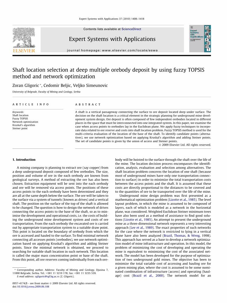
If jV j ¼ 3 the SMT can be directly constructed as follows: LetV ¼ fa; b; cg

1. If one of the angles of Dabc is at least 120�, then the SMT con-sists of simply two edges subtending the obtuse angle.

2. Assume that all internal angles of Dabc are less than 120�. Now,we can draw an equilateral triangle Dabd and circumscribe acircle around this triangle. The intersection of line ½c; d� withthe circle circumscribing the three points a; b and d is the Stei-ner point s. Hence the location of s is determined, see Fig. 4a.The FST for a three given points involves segments as, bs andcs whose total length is equal to the length of segment cd. Thesegment cd is known as the Simpson line for the FST over termi-nals a; b and c.

A

(a)

D

C (b)

B

S

Fig. 4. (a) A 3-point SMT algorithm, (b) the SMT for three points at vertices of anequilateral triangle.

Table 1The transformation of linguistic terms to positive triangular fuzzy numbers.

Description Fuzzy number

VL (30,40,50) or (0.3,0.4,0.5)L (40,50,60) or (0.4,0.5,0.6)M (50,60,70) or (0.5,0.6,0.7)H (60,70,80) or (0.6,0.7,0.8)VH (70,80,90) or (0.7,0.8,0.9)

0.8

0.9

1

VL

L

Z. Gligoric et al. / Expert Systems with Applications 37 (2010) 1408–1418 1411

The step that substitutes d for a and b will be called the mergingstage, and the step that locates s and adds the connections ½a; s� and½b; s� is the reconstruction stage.

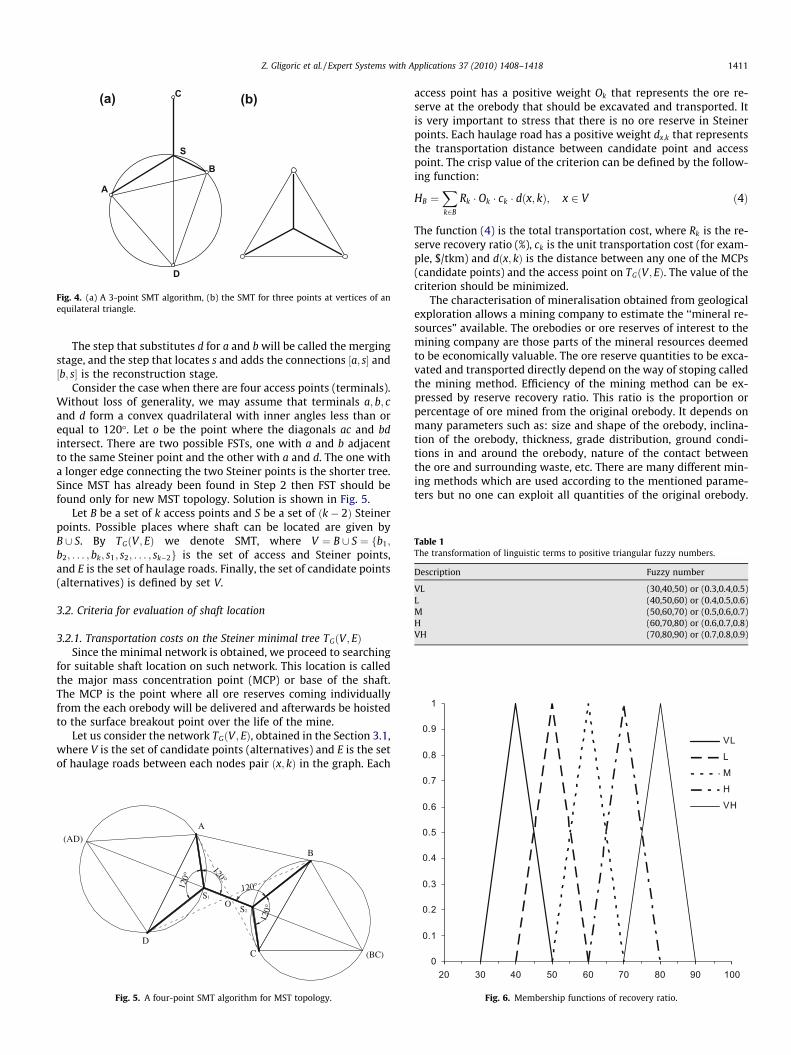
Consider the case when there are four access points (terminals).Without loss of generality, we may assume that terminals a; b; cand d form a convex quadrilateral with inner angles less than orequal to 120�. Let o be the point where the diagonals ac and bdintersect. There are two possible FSTs, one with a and b adjacentto the same Steiner point and the other with a and d. The one witha longer edge connecting the two Steiner points is the shorter tree.Since MST has already been found in Step 2 then FST should befound only for new MST topology. Solution is shown in Fig. 5.

Let B be a set of k access points and S be a set of ðk� 2Þ Steinerpoints. Possible places where shaft can be located are given byB [ S. By TGðV ; EÞ we denote SMT, where V ¼ B [ S ¼ fb1;

b2; . . . ; bk; s1; s2; . . . ; sk�2g is the set of access and Steiner points,and E is the set of haulage roads. Finally, the set of candidate points(alternatives) is defined by set V.

3.2. Criteria for evaluation of shaft location

3.2.1. Transportation costs on the Steiner minimal tree TGðV ; EÞSince the minimal network is obtained, we proceed to searching

for suitable shaft location on such network. This location is calledthe major mass concentration point (MCP) or base of the shaft.The MCP is the point where all ore reserves coming individuallyfrom the each orebody will be delivered and afterwards be hoistedto the surface breakout point over the life of the mine.

Let us consider the network TGðV ; EÞ, obtained in the Section 3.1,where V is the set of candidate points (alternatives) and E is the setof haulage roads between each nodes pair ðx; kÞ in the graph. Each

120°

120°

120°

120°

A

B

CD

O

(AD)

(BC)

S1

S2

Fig. 5. A four-point SMT algorithm for MST topology.

access point has a positive weight Ok that represents the ore re-serve at the orebody that should be excavated and transported. Itis very important to stress that there is no ore reserve in Steinerpoints. Each haulage road has a positive weight dx;k that representsthe transportation distance between candidate point and accesspoint. The crisp value of the criterion can be defined by the follow-ing function:

HB ¼Xk2B

Rk � Ok � ck � dðx; kÞ; x 2 V ð4Þ

The function (4) is the total transportation cost, where Rk is the re-serve recovery ratio (%), ck is the unit transportation cost (for exam-ple, $/tkm) and dðx; kÞ is the distance between any one of the MCPs(candidate points) and the access point on TGðV ; EÞ. The value of thecriterion should be minimized.

The characterisation of mineralisation obtained from geologicalexploration allows a mining company to estimate the ‘‘mineral re-sources” available. The orebodies or ore reserves of interest to themining company are those parts of the mineral resources deemedto be economically valuable. The ore reserve quantities to be exca-vated and transported directly depend on the way of stoping calledthe mining method. Efficiency of the mining method can be ex-pressed by reserve recovery ratio. This ratio is the proportion orpercentage of ore mined from the original orebody. It depends onmany parameters such as: size and shape of the orebody, inclina-tion of the orebody, thickness, grade distribution, ground condi-tions in and around the orebody, nature of the contact betweenthe ore and surrounding waste, etc. There are many different min-ing methods which are used according to the mentioned parame-ters but no one can exploit all quantities of the original orebody.

0

0.1

0.2

0.3

0.4

0.5

0.6

0.7

20 30 40 50 60 70 80 90 100

M

H

VH

Fig. 6. Membership functions of recovery ratio.

1412 Z. Gligoric et al. / Expert Systems with Applications 37 (2010) 1408–1418

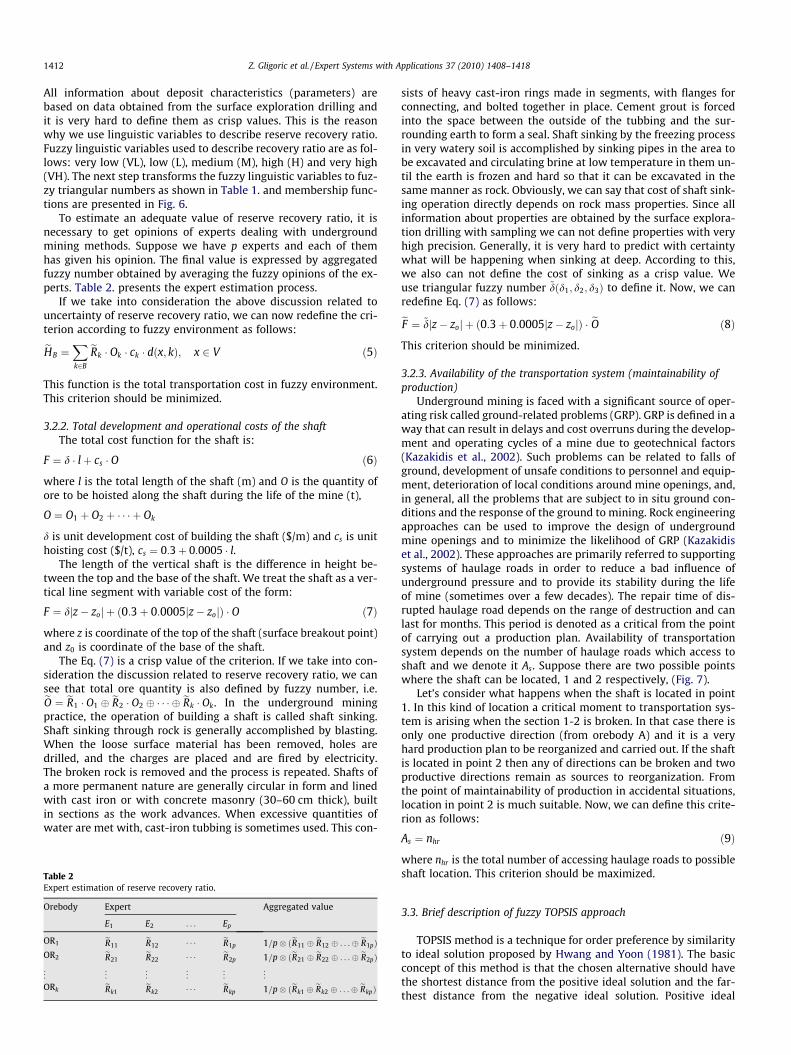
All information about deposit characteristics (parameters) arebased on data obtained from the surface exploration drilling andit is very hard to define them as crisp values. This is the reasonwhy we use linguistic variables to describe reserve recovery ratio.Fuzzy linguistic variables used to describe recovery ratio are as fol-lows: very low (VL), low (L), medium (M), high (H) and very high(VH). The next step transforms the fuzzy linguistic variables to fuz-zy triangular numbers as shown in Table 1. and membership func-tions are presented in Fig. 6.

To estimate an adequate value of reserve recovery ratio, it isnecessary to get opinions of experts dealing with undergroundmining methods. Suppose we have p experts and each of themhas given his opinion. The final value is expressed by aggregatedfuzzy number obtained by averaging the fuzzy opinions of the ex-perts. Table 2. presents the expert estimation process.

If we take into consideration the above discussion related touncertainty of reserve recovery ratio, we can now redefine the cri-terion according to fuzzy environment as follows:eHB ¼

Xk2B

eRk � Ok � ck � dðx; kÞ; x 2 V ð5Þ

This function is the total transportation cost in fuzzy environment.This criterion should be minimized.

3.2.2. Total development and operational costs of the shaftThe total cost function for the shaft is:

F ¼ d � lþ cs � O ð6Þ

where l is the total length of the shaft (m) and O is the quantity ofore to be hoisted along the shaft during the life of the mine (t),

O ¼ O1 þ O2 þ � � � þ Ok

d is unit development cost of building the shaft ($/m) and cs is unithoisting cost ($/t), cs ¼ 0:3þ 0:0005 � l.

The length of the vertical shaft is the difference in height be-tween the top and the base of the shaft. We treat the shaft as a ver-tical line segment with variable cost of the form:

F ¼ djz� zoj þ ð0:3þ 0:0005jz� zojÞ � O ð7Þ

where z is coordinate of the top of the shaft (surface breakout point)and z0 is coordinate of the base of the shaft.

The Eq. (7) is a crisp value of the criterion. If we take into con-sideration the discussion related to reserve recovery ratio, we cansee that total ore quantity is also defined by fuzzy number, i.e.eO ¼ eR1 � O1 � eR2 � O2 � � � � � eRk � Ok. In the underground miningpractice, the operation of building a shaft is called shaft sinking.Shaft sinking through rock is generally accomplished by blasting.When the loose surface material has been removed, holes aredrilled, and the charges are placed and are fired by electricity.The broken rock is removed and the process is repeated. Shafts ofa more permanent nature are generally circular in form and linedwith cast iron or with concrete masonry (30–60 cm thick), builtin sections as the work advances. When excessive quantities ofwater are met with, cast-iron tubbing is sometimes used. This con-

Table 2Expert estimation of reserve recovery ratio.

Orebody Expert Aggregated value

E1 E2 . . . Ep

OR1 eR11eR12

. . . eR1p 1=p� ðeR11 � eR12 � . . .� eR1pÞOR2 eR21

eR22. . . eR2p 1=p� ðeR21 � eR22 � . . .� eR2pÞ

..

. ... ..

. ... ..

. ...

ORk eRk1eRk2

. . . eRkp 1=p� ðeRk1 � eRk2 � . . .� eRkpÞ

sists of heavy cast-iron rings made in segments, with flanges forconnecting, and bolted together in place. Cement grout is forcedinto the space between the outside of the tubbing and the sur-rounding earth to form a seal. Shaft sinking by the freezing processin very watery soil is accomplished by sinking pipes in the area tobe excavated and circulating brine at low temperature in them un-til the earth is frozen and hard so that it can be excavated in thesame manner as rock. Obviously, we can say that cost of shaft sink-ing operation directly depends on rock mass properties. Since allinformation about properties are obtained by the surface explora-tion drilling with sampling we can not define properties with veryhigh precision. Generally, it is very hard to predict with certaintywhat will be happening when sinking at deep. According to this,we also can not define the cost of sinking as a crisp value. Weuse triangular fuzzy number ~dðd1; d2; d3Þ to define it. Now, we canredefine Eq. (7) as follows:eF ¼ ~djz� zoj þ ð0:3þ 0:0005jz� zojÞ � eO ð8Þ

This criterion should be minimized.

3.2.3. Availability of the transportation system (maintainability ofproduction)

Underground mining is faced with a significant source of oper-ating risk called ground-related problems (GRP). GRP is defined in away that can result in delays and cost overruns during the develop-ment and operating cycles of a mine due to geotechnical factors(Kazakidis et al., 2002). Such problems can be related to falls ofground, development of unsafe conditions to personnel and equip-ment, deterioration of local conditions around mine openings, and,in general, all the problems that are subject to in situ ground con-ditions and the response of the ground to mining. Rock engineeringapproaches can be used to improve the design of undergroundmine openings and to minimize the likelihood of GRP (Kazakidiset al., 2002). These approaches are primarily referred to supportingsystems of haulage roads in order to reduce a bad influence ofunderground pressure and to provide its stability during the lifeof mine (sometimes over a few decades). The repair time of dis-rupted haulage road depends on the range of destruction and canlast for months. This period is denoted as a critical from the pointof carrying out a production plan. Availability of transportationsystem depends on the number of haulage roads which access toshaft and we denote it As. Suppose there are two possible pointswhere the shaft can be located, 1 and 2 respectively, (Fig. 7).

Let’s consider what happens when the shaft is located in point1. In this kind of location a critical moment to transportation sys-tem is arising when the section 1-2 is broken. In that case there isonly one productive direction (from orebody A) and it is a veryhard production plan to be reorganized and carried out. If the shaftis located in point 2 then any of directions can be broken and twoproductive directions remain as sources to reorganization. Fromthe point of maintainability of production in accidental situations,location in point 2 is much suitable. Now, we can define this crite-rion as follows:

As ¼ nhr ð9Þ

where nhr is the total number of accessing haulage roads to possibleshaft location. This criterion should be maximized.

3.3. Brief description of fuzzy TOPSIS approach

TOPSIS method is a technique for order preference by similarityto ideal solution proposed by Hwang and Yoon (1981). The basicconcept of this method is that the chosen alternative should havethe shortest distance from the positive ideal solution and the far-thest distance from the negative ideal solution. Positive ideal

21from ore body A

from

ore

body

B

fromore

body C

21from ore body A

from

ore

body

B

fromore

body C

Fig. 7. Candidate points to shaft location.

Z. Gligoric et al. / Expert Systems with Applications 37 (2010) 1408–1418 1413

solution is a solution that maximizes the benefit criteria and min-imizes cost criteria, whereas the negative ideal solution maximizesthe cost criteria and minimizes the benefit criteria (Wang & Elhag,2006). In the classical TOPSIS method, the weights of the criteriaand the ratings of alternatives are known precisely and crisp valuesare used in the evaluation process. However, under many condi-tions crisp data are inadequate to describe real-life decision prob-lems. In such cases, the fuzzy TOPSIS method is proposed wherethe weights of criteria and ratings of alternatives are evaluatedby linguistic variables represented by fuzzy numbers.

There are many applications of fuzzy TOPSIS in the literature.For instance, Chen (2000) extended the TOPSIS to the fuzzy envi-ronment and gave numerical example of system analysis engineerselection for a software company. Chu (2002) presented a fuzzyTOPSIS model under group decisions for solving the facility loca-tion selection problem. Yang and Hung (2007) proposed to useTOPSIS and fuzzy TOPSIS methods for plant layout design problem.In general, a multiple criteria decision making problem can be con-cisely expressed in matrix format as:

ð10Þ

where A1;A2; . . . ;Am are possible alternatives, C1; C2; . . . ;Cn are crite-ria which measure the performance of alternatives and ~xij is the rat-ing of alternative Ai with respect to criteria Cj. In this paper, therating of alternative Ai with respect to criteria C1 and C2 are repre-sented as triangular fuzzy numbers.

The fuzzy TOPSIS method is based on the following steps.

Step 1. Construct the normalized decision matrix eRThe first step concerns the normalization of the judgment ma-

trix eD ¼ j~xijj. Each element ~xij is transformed using the followingequation

~rij ¼~xijffiffiffiffiffiffiffiffiffiffiffiffiffiffiffiPm

i¼1~x2ij

q ¼ ðaij; bij; cijÞffiffiffiffiffiffiffiffiffiffiffiffiffiffiffiffiffiffiffiffiffiffiffiffiffiffiffiffiffiffiffiffiffiffiffiPmi¼1ðaij; bij; cijÞ2

q j ¼ 1;2; . . . ; n ð11Þ

The normalized decision matrix is as follows:

eR ¼ ~rij

�� �� ¼~r11 ~r12 ~r13 � � � ~r1n

~r21 ~r22 ~r23 � � � ~r2n

~r31 ~r32 ~r33 � � � ~r3n

..

. ... ..

. . .. ..

.

~rm1 ~rm2 ~rm3 � � � ~rmn

�������������

�������������ð12Þ

Step 2. Construct the weighted normalized decision matrix eV

Criteria importance is a reflection of the decision maker’s sub-

jective preference as well as the objective characteristics of the cri-teria themselves (Zeleney, 1982). In order to determine criteriaimportance, we applied concept of the entropy method. Shannonand Weaver (1947) proposed the entropy concept and this concepthas been highlighted by Zeleney (1982) for deciding the objectiveweights of criteria. Entropy is a measure of uncertainty in the infor-mation formulated using probability theory. To determine weightsby the entropy measure, the normalized decision matrix eR ¼ j~rijjgiven by Eq. (12) is considered. The amount of decision informationcontained in Eq. (12) and associated with each criterion can bemeasured by the entropy value ej as:

ej ¼ �kXm

i¼1

rij � ln rij ð13Þ

where k ¼ 1= ln m is a constant that guarantees 0 6 ej 6 1. The de-gree of divergence ðdijÞ of the average information contained byeach criterion Cjðj ¼ 1;2; . . . ;nÞ can be calculated as:

dj ¼ 1� ej ð14Þ

The objective weight for each criterion Cjðj ¼ 1;2; . . . ;nÞ is thus gi-ven by:

wj ¼ dj

Xn

j¼1dj

.ð15Þ

Finally the weighted normalized decision matrix is as follows:

eV ¼ j~rij ~wjj ¼

~r11 ~w1 ~r12 ~w2 ~r13 ~w3 � � � ~r1n ~wn

~r21 ~w1 ~r22 ~w2 ~r23 ~w3 � � � ~r2n ~wn

~r31 ~w1 ~r32 ~w2 ~r33 ~w3 � � � ~r3n ~wn

..

. ... ..

. . .. ..

.

~rm1 ~w1 ~rm2 ~w2 ~rm3 ~w3 � � � ~rmn ~wn

��������������

��������������ð16Þ

Step 3. Define the ideal and the negative-ideal solutions

Let us suppose that eAþ identifies the ideal solution and eA� thenegative one. They are defined as follows:

eAþ ¼ max ~v ijjj 2 Ji¼1;2;...;m

!; min ~v ijjj 2 J0

i¼1;2;::;m

!( )¼ ~vþ1 ; ~vþ2 ; . . . ; ~vþn� �

ð17Þ

eA� ¼ min ~v ijjj 2 Ji¼1;2;...;m

!; max ~v ijjj 2 J0

i¼1;2;::;m

!( )¼ ~v�1 ; ~v�2 ; . . . ; ~v�n� �

ð18Þ

where {J ¼ fj ¼ 1;2; . . . ;njj associated with the benefit criteria and{J0 ¼ fj ¼ 1;2; . . . ;njj associated with the cost criteria}.

0

500

1000

1500

2000

2500

3500

4000

4500

3000

0

500

1000

1500

2000

2500

3000

3500

4000

4500

AB

C

D

2

3

4

1

425

400

375

350

325

300

275300325

523053 350

Fig. 8. Initial graph.

3000

3500

4500

4000400A

1 B

425

Table 3Operational data.

Access point (x,y,z)Orebody A (1) (1500;3500;�300)Orebody B (2) (4000;3000;�300)Orebody C (3) (3000;1000;�300)Orebody D (4) (500;2000;�300)

Ore reserveOrebody A 3 592 463 tOrebody B 1 606 334 tOrebody C 2 084 292 tOrebody D 1 976 486 tMining method (Room and pillar) & reserve recovery ratio – expert estimationOrebody A L = (0.4,0.5,0.6) M = (0.5,0.6,0.7) M = (0.5,0.6,0.7) (0.46,0.56,0.66) aggregated numberOrebody B M = (0.5,0.6,0.7) L = (0.4,0.5,0.6) H = (0.6,0.7,0.8) (0.50,0.60,0.70) aggregated numberOrebody C M = (0.5,0.6,0.7) H = (0.6,0.7,0.8) H = (0.6,0.7,0.8) (0.56,0.66,0.76) aggregated numberOrebody D VH = (0.7,0.8, 0.9) H = (0.6,0.7,0.8) H = (0.6,0.7,0.8) (0.63,0.73,0.83) aggregated numberCostHaulage & HoistDrive (haul truck) 0.8 $/tkm = 0.0008 $/tmShaft (skip system) (0.3 + 0.0005 Length) $/t

BuildingShaft (16,000,18,000,22,000) $/m

1414 Z. Gligoric et al. / Expert Systems with Applications 37 (2010) 1408–1418

With benefit and cost attributes, we discriminate between cri-teria that the decision maker desires to maximize or minimize,respectively.

Step 4. Measure the distance between alternatives and idealsolutions

To calculate the n-Euclidean distance from each alternative toeAþ and eA� the following equations can be easily adopted:

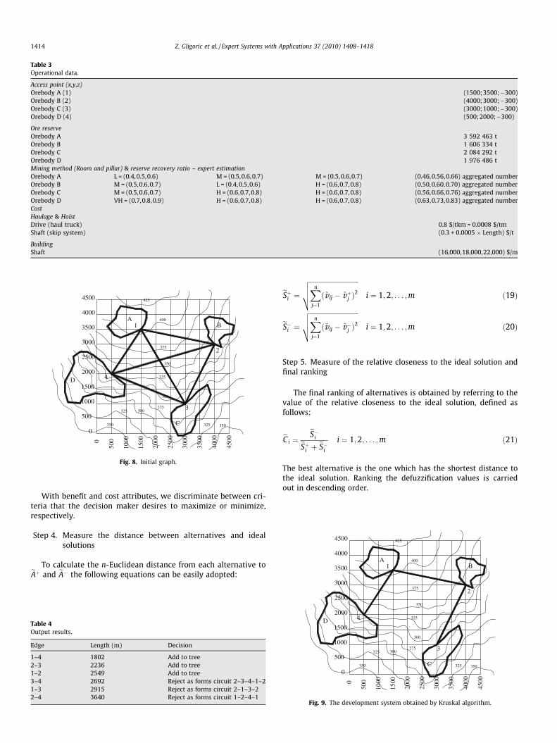
Table 4Output results.

Edge Length (m) Decision

1–4 1802 Add to tree2–3 2236 Add to tree1–2 2549 Add to tree3–4 2692 Reject as forms circuit 2–3–4–1–21–3 2915 Reject as forms circuit 2–1–3–22–4 3640 Reject as forms circuit 1–2–4–1

eSþi ¼ffiffiffiffiffiffiffiffiffiffiffiffiffiffiffiffiffiffiffiffiffiffiffiffiffiffiffiffiffiffiXn

j¼1

ð~v ij � ~vþj Þ2

vuut i ¼ 1;2; . . . ;m ð19Þ

eS�i ¼ffiffiffiffiffiffiffiffiffiffiffiffiffiffiffiffiffiffiffiffiffiffiffiffiffiffiffiffiffiffiXn

j¼1

ð~v ij � ~v�j Þ2

vuut i ¼ 1;2; . . . ;m ð20Þ

Step 5. Measure of the relative closeness to the ideal solution andfinal ranking

The final ranking of alternatives is obtained by referring to thevalue of the relative closeness to the ideal solution, defined asfollows:

eCi ¼eS�ieSþi þ eS�i i ¼ 1;2; . . . ;m ð21Þ

The best alternative is the one which has the shortest distance tothe ideal solution. Ranking the defuzzification values is carriedout in descending order.

3254D

325

1000

0

5000

1000

500350

1500

3500

2000

1500

3000

2500

4500

4000

275 3300

C

300

350325

2500

2000

375

350

2

Fig. 9. The development system obtained by Kruskal algorithm.

D 4 325

0

0

1000

500

1500

1500

500

1000

2500

2000

4000

3000

3500

4500

C

275300

350

325

300

3

325 350

2000

2500

3000

3500

4000

4500

A 400

375

350

1

2

B

425

4

3

S1

S2

1

2

Fig. 10. Steiner minimal tree and locations of Steiner pointsS1ð1574;2775;�300Þ; S2ð2878;2190;�300Þ.

Table 5Description of alternatives.

Alternative Base of the shaft (x,y,z) Top of the shaft (x,y,z) Length (m)

Shaft 1 1500, 3500, �300 1500, 3500, 404 704Shaft 2 4000, 3000, �300 4000, 3000, 340 640Shaft 3 3000, 1000, �300 3000, 1000, 288 588Shaft 4 500, 2000, �300 500, 2000, 330 630Shaft 5 1574, 2775, �300 1574, 2775, 377 677Shaft 6 2878, 2190, �300 2878, 2190, 347 647

Z. Gligoric et al. / Expert Systems with Applications 37 (2010) 1408–1418 1415

4. Application of procedure

4.1. A numerical example statement

To illustrate the proposed procedure, we applied it to a caseconsidering the design of an underground mine development sys-tem. The Cu deposit is to be developed, the situation is hypotheti-cal and the numbers used are in to permit calculation. Thehypothetical deposit includes four orebodies, A through D with ac-cess points k ¼ 1;2;3;4 respectively. The relevant operational dataare shown in Table 3.

4.2. Numerical example solution

The initial graph containing all possible paths between accesspoints is shown in Fig. 8. Applying Kruskal’s algorithm and startingwith the shortest edge, we have output results as shown in Table 4.

Stop as three edges have been added and these are all we needfor the MST of a graph with four access points. Hence the MST of

0-1000

500 1

-500

0

500

1000

500

1000

1500

2000

2500

3000

3500

1

4

S1shaf

t 1sh

aft 4

shaf

t 5

Fig. 11. Alternatives

the graph shown above consists of the edges 1–4; 2–3; 1–2 withtotal length of 6587 m and it is as shown in Fig. 9.

As we are allowed to add new nodes to the graph, we are thenlooking for the shortest Steiner tree and these new nodes are calledSteiner points. Fig. 10. shows the SMT and S1; S2 nodes in the figurerepresent Steiner points. Total length of the development systemobtained by SMT is 6063 m and the Steiner ratio is 10,864. Accord-ing to Fig. 10. the set of candidate points (alternatives) to shaftlocation is defined by V ¼ f1;2;3;4; S1; S2g. Finally, we have sixalternatives (Fig. 11) with following characteristics shown in Table5 (see Table 6).

Criterion C1 (transportation costs on TGðV ; EÞ). To calculate trans-portation costs on TGðV ; EÞ, we used following algorithm: Step 1.Obtain the minimum distance matrix for the candidate points ofTG. Step 2. Multiply the j-th column of the minimum distance ma-trix by the ore reserve and unit haulage cost cjðj ¼ 1;2; . . . ;nÞ to ob-tain the haulage cost matrix eH ¼ keRj � Oj � cj � dijkn

1. Step 3. For eachrow of the eH matrix, compute the sum of all the terms in the row.The distance matrix is given:

DM ¼

from=to 1 2 3 4 S1 S2

1 0 3542 3355 2054 729 21592 3542 0 2579 4138 2813 13833 3355 2579 0 3951 2626 11964 2054 4138 3951 0 1325 2755S1 729 2813 2626 1325 0 1430S2 2159 1383 1196 2755 1430 0

000 1500 2000 2500 3000 3500 4000

2

3

S2

shaf

t 2

shaf

t 3

shaf

t 6

to shaft location.

1416 Z. Gligoric et al. / Expert Systems with Applications 37 (2010) 1408–1418

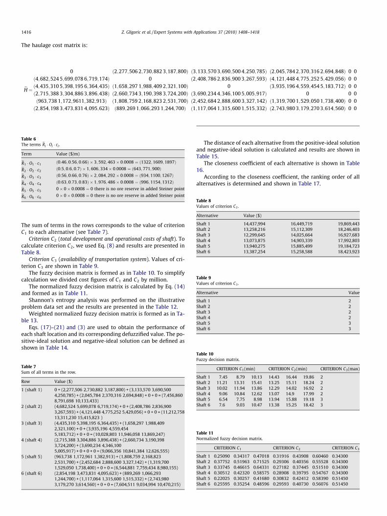
The haulage cost matrix is:

eH¼0 ð2;277;506 2;730;882 3;187;800Þ ð3;133;570 3;690;500 4;250;785Þ ð2;045;784 2;370;316 2;694;848Þ 0 0

ð4;682;524 5;699;078 6;719;174Þ 0 ð2;408;786 2;836;900 3;267;593Þ ð4;121;448 4;775;252 5;429;056Þ 0 0ð4;435;310 5;398;195 6;364;435Þ ð1;658;297 1;988;409 2;321;100Þ 0 ð3;935;196 4;559;454 5;183;712Þ 0 0ð2;715;388 3;304;886 3;896;438Þ ð2;660;734 3;190;398 3;724;200Þ ð3;690;234 4;346;100 5;005;917Þ 0 0 0ð963;738 1;172;9611;382;913Þ ð1;808;759 2;168;823 2;531;700Þ ð2;452;684 2;888;600 3;327;142Þ ð1;319;700 1;529;050 1;738;400Þ 0 0ð2;854;198 3;473;831 4;095;623Þ ð889;269 1;066;293 1;244;700Þ ð1;117;064 1;315;600 1;515;332Þ ð2;743;980 3;179;270 3;614;560Þ 0 0

Table 8Values of criterion C2.

Alternative Value ($)

Shaft 1 14,437,994 16,449,719 19,869,443Shaft 2 13,258,216 15,112,309 18,246,403Shaft 3 12,299,645 14,025,664 16,927,683Shaft 4 13,073,875 14,903,339 17,992,803Shaft 5 13,940,275 15,885,499 19,184,723Shaft 6 13,387,254 15,258,588 18,423,923

Table 9Values of criterion C3.

Alternative Value

Shaft 1 2Shaft 2 2Shaft 3 2Shaft 4 2Shaft 5 3Shaft 6 3

Table 6The terms eRj � Oj � cj .

Term Value ($/m)

eR1 � O1 � c1ð0:46; 0:56;0:66Þ 3;592;463 0:0008 ¼ ð1322;1609;1897ÞeR2 � O2 � c2ð0:5;0:6; 0:7Þ 1;606;334 0:0008 ¼ ð643;771;900ÞeR3 � O3 � c3ð0:56; 0:66;0:76Þ 2;084;292 0:0008 ¼ ð934;1100;1267ÞeR4 � O4 � c4ð0:63; 0:73;0:83Þ 1;976;486 0:0008 ¼ ð996;1154;1312ÞeR5 � O5 � c50 0 0:0008 ¼ 0 there is no ore reserve in added Steiner pointeR6 � O6 � c60 0 0:0008 ¼ 0 there is no ore reserve in added Steiner point

The sum of terms in the rows corresponds to the value of criterionC1 to each alternative (see Table 7).

Criterion C2 (total development and operational costs of shaft). Tocalculate criterion C2, we used Eq. (8) and results are presented inTable 8.

Criterion C3 (availability of transportation system). Values of cri-terion C3 are shown in Table 9.

The fuzzy decision matrix is formed as in Table 10. To simplifycalculation we divided cost figures of C1 and C2 by million.

The normalized fuzzy decision matrix is calculated by Eq. (14)and formed as in Table 11.

Shannon’s entropy analysis was performed on the illustrativeproblem data set and the results are presented in the Table 12.

Weighted normalized fuzzy decision matrix is formed as in Ta-ble 13.

Eqs. (17)–(21) and (3) are used to obtain the performance ofeach shaft location and its corresponding defuzzified value. The po-sitive-ideal solution and negative-ideal solution can be defined asshown in Table 14.

Table 7Sum of all terms in the row.

Row Value ($)

1 (shaft 1) 0 + (2,277,506 2,730,882 3,187,800) + (3,133,570 3,690,5004,250,785) + (2,045,784 2,370,316 2,694,848) + 0 + 0 = (7,456,8608,791,698 10,133,433)

2 (shaft 2) (4,682,524 5,699,078 6,719,174) + 0 + (2,408,786 2,836,9003,267,593) + (4,121,448 4,775,252 5,429,056) + 0 + 0 = (11,212,75813,311,230 15,415,823 )

3 (shaft 3) (4,435,310 5,398,195 6,364,435) + (1,658,297 1,988,4092,321,100) + 0 + (3,935,196 4,559,4545,183,712) + 0 + 0 = (10,028,803 11,946,058 13,869,247)

4 (shaft 4) (2,715,388 3,304,886 3,896,438) + (2,660,734 3,190,3983,724,200) + (3,690,234 4,346,1005,005,917) + 0 + 0 + 0 = (9,066,356 10,841,384 12,626,555)

5 (shaft 5) (963,738 1,172,961 1,382,913) + (1,808,759 2,168,8232,531,700) + (2,452,684 2,888,600 3,327,142) + (1,319,7001,529,050 1,738,400) + 0 + 0 = (6,544,881 7,759,434 8,980,155)

6 (shaft 6) (2,854,198 3,473,831 4,095,623) + (889,269 1,066,2931,244,700) + (1,117,064 1,315,600 1,515,332) + (2,743,9803,179,270 3,614,560) + 0 + 0 = (7,604,511 9,034,994 10,470,215)

The distance of each alternative from the positive-ideal solutionand negative-ideal solution is calculated and results are shown inTable 15.

The closeness coefficient of each alternative is shown in Table16.

According to the closeness coefficient, the ranking order of allalternatives is determined and shown in Table 17.

Table 10Fuzzy decision matrix.

CRITERION C1(min) CRITERION C2(min) CRITERION C3(max)

Shaft 1 7.45 8.79 10.13 14.43 16.44 19.86 2Shaft 2 11.21 13.31 15.41 13.25 15.11 18.24 2Shaft 3 10.02 11.94 13.86 12.29 14.02 16.92 2Shaft 4 9.06 10.84 12.62 13.07 14.9 17.99 2Shaft 5 6.54 7.75 8.98 13.94 15.88 19.18 3Shaft 6 7.6 9.03 10.47 13.38 15.25 18.42 3

Table 11Normalized fuzzy decision matrix.

CRITERION C1 CRITERION C2 CRITERION C3

Shaft 1 0.25090 0.34317 0.47018 0.31916 0.43908 0.60460 0.34300Shaft 2 0.37752 0.51963 0.71525 0.29306 0.40356 0.55528 0.34300Shaft 3 0.33745 0.46615 0.64331 0.27182 0.37445 0.51510 0.34300Shaft 4 0.30512 0.42320 0.58575 0.28908 0.39795 0.54767 0.34300Shaft 5 0.22025 0.30257 0.41680 0.30832 0.42412 0.58390 0.51450Shaft 6 0.25595 0.35254 0.48596 0.29593 0.40730 0.56076 0.51450

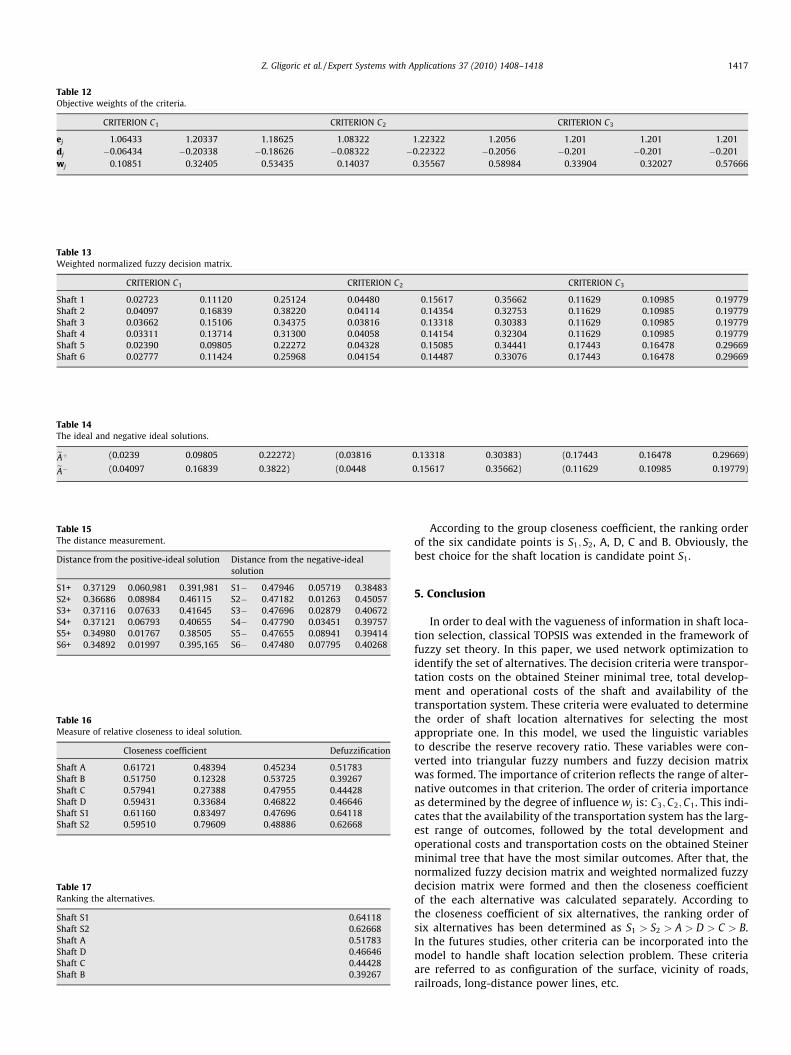
Table 12Objective weights of the criteria.

CRITERION C1 CRITERION C2 CRITERION C3

ej 1.06433 1.20337 1.18625 1.08322 1.22322 1.2056 1.201 1.201 1.201dj �0.06434 �0.20338 �0.18626 �0.08322 �0.22322 �0.2056 �0.201 �0.201 �0.201wj 0.10851 0.32405 0.53435 0.14037 0.35567 0.58984 0.33904 0.32027 0.57666

Table 13Weighted normalized fuzzy decision matrix.

CRITERION C1 CRITERION C2 CRITERION C3

Shaft 1 0.02723 0.11120 0.25124 0.04480 0.15617 0.35662 0.11629 0.10985 0.19779Shaft 2 0.04097 0.16839 0.38220 0.04114 0.14354 0.32753 0.11629 0.10985 0.19779Shaft 3 0.03662 0.15106 0.34375 0.03816 0.13318 0.30383 0.11629 0.10985 0.19779Shaft 4 0.03311 0.13714 0.31300 0.04058 0.14154 0.32304 0.11629 0.10985 0.19779Shaft 5 0.02390 0.09805 0.22272 0.04328 0.15085 0.34441 0.17443 0.16478 0.29669Shaft 6 0.02777 0.11424 0.25968 0.04154 0.14487 0.33076 0.17443 0.16478 0.29669

Table 14The ideal and negative ideal solutions.

eAþ (0.0239 0.09805 0.22272) (0.03816 0.13318 0.30383) (0.17443 0.16478 0.29669)eA� (0.04097 0.16839 0.3822) (0.0448 0.15617 0.35662) (0.11629 0.10985 0.19779)

Table 15The distance measurement.

Distance from the positive-ideal solution Distance from the negative-idealsolution

S1+ 0.37129 0.060,981 0.391,981 S1� 0.47946 0.05719 0.38483S2+ 0.36686 0.08984 0.46115 S2� 0.47182 0.01263 0.45057S3+ 0.37116 0.07633 0.41645 S3� 0.47696 0.02879 0.40672S4+ 0.37121 0.06793 0.40655 S4� 0.47790 0.03451 0.39757S5+ 0.34980 0.01767 0.38505 S5� 0.47655 0.08941 0.39414S6+ 0.34892 0.01997 0.395,165 S6� 0.47480 0.07795 0.40268

Table 16Measure of relative closeness to ideal solution.

Closeness coefficient Defuzzification

Shaft A 0.61721 0.48394 0.45234 0.51783Shaft B 0.51750 0.12328 0.53725 0.39267Shaft C 0.57941 0.27388 0.47955 0.44428Shaft D 0.59431 0.33684 0.46822 0.46646Shaft S1 0.61160 0.83497 0.47696 0.64118Shaft S2 0.59510 0.79609 0.48886 0.62668

Table 17Ranking the alternatives.

Shaft S1 0.64118Shaft S2 0.62668Shaft A 0.51783Shaft D 0.46646Shaft C 0.44428Shaft B 0.39267

Z. Gligoric et al. / Expert Systems with Applications 37 (2010) 1408–1418 1417

According to the group closeness coefficient, the ranking orderof the six candidate points is S1; S2, A, D, C and B. Obviously, thebest choice for the shaft location is candidate point S1.

5. Conclusion

In order to deal with the vagueness of information in shaft loca-tion selection, classical TOPSIS was extended in the framework offuzzy set theory. In this paper, we used network optimization toidentify the set of alternatives. The decision criteria were transpor-tation costs on the obtained Steiner minimal tree, total develop-ment and operational costs of the shaft and availability of thetransportation system. These criteria were evaluated to determinethe order of shaft location alternatives for selecting the mostappropriate one. In this model, we used the linguistic variablesto describe the reserve recovery ratio. These variables were con-verted into triangular fuzzy numbers and fuzzy decision matrixwas formed. The importance of criterion reflects the range of alter-native outcomes in that criterion. The order of criteria importanceas determined by the degree of influence wj is: C3;C2;C1. This indi-cates that the availability of the transportation system has the larg-est range of outcomes, followed by the total development andoperational costs and transportation costs on the obtained Steinerminimal tree that have the most similar outcomes. After that, thenormalized fuzzy decision matrix and weighted normalized fuzzydecision matrix were formed and then the closeness coefficientof the each alternative was calculated separately. According tothe closeness coefficient of six alternatives, the ranking order ofsix alternatives has been determined as S1 > S2 > A > D > C > B.In the futures studies, other criteria can be incorporated into themodel to handle shaft location selection problem. These criteriaare referred to as configuration of the surface, vicinity of roads,railroads, long-distance power lines, etc.

1418 Z. Gligoric et al. / Expert Systems with Applications 37 (2010) 1408–1418

References

Bellman, R. E., & Zadeh, L. A. (1977). Local and fuzzy logics. In J. M. Dunn & G. Epstein(Eds.), Modern uses of multiple-valued logic (pp. 105–151). Boston: Kluwer. 158–165.

Bojadziev, G., & Bojadziev, M. (1998). Fuzzy sets and fuzzy logic applications.Singapore: World Scientific.

Brazil, M., Thomas, D. A & Weng, J. F. (1998). Gradient constrained minimal steinertrees, in network design: Connectivity and facilities location (DIMACS Series inDiscrete Mathematics and Theoretical Computer Science, 40) (pp. 23- 38).Providence: American Mathematical Society.

Brazil, M., Thomas, D. A., Weng, J. F., et al. (2005). Cost optimization for undergroundmining networks (pp. 241–256), Optimization and engineering 6. SpringerScience Business Media, Inc., Manufactured in The Netherlands, 2005.

Brazil, M., Lee, H., Rubinstein, H., Thomas, D., Weng, J., Wormald, C., et al. (2000).Network optimization of underground mine design. The AusIMM Proceedings, 1,57–65.

Brazil, M., Lee, D. H., Van Leuven, M., Rubinstein, J. H., Thomas, D. A., & Wormald, N.C. (2003). Optimising declines in underground mines. Transactions of theInstitutions of Mining and Metallurgy, Section A: Mining technology, 164–170.

Chen, C. T. (2000). Extension of the TOPSIS for group decision making under fuzzyenvironment. Fuzzy Sets and Systems, 114, 1–9.

Chu, T. C. (2002). Selecting plant location via a fuzzy TOPSIS approach. TheInternational Journal of Advanced Manufacturing Technology, 20, 859–864.

Gertsbakh, I., Shpungin, Y., et al. (2004). Combinatorial approaches to Monte Carloestimation of network lifetime distribution. Applied Stochastics Models inBusiness and Industry, 49–57.

Hwang, F. K., Richards, D. S., Winter, P., et al. (1992). The steiner tree problem. Annalsof discrete mathematics. Elsevier Science Publishers B.V.

Hwang, C. L., & Yoon, K. (1981). Multiple attribute decision making: Methods andapplications. Berlin: Springer.

Kaufmann, A., & Gupta, M. M. (1985). Introduction to fuzzy arithmetic: Theory andapplications. New York: Van Nostrand Reinhold.

Kazakidis, V. N., Scoble, M., et al. (2002). Accounting for ground-related problems inmine production system planning. Mineral Resources Engineering, 11(1), 35–57.

Kruskal, J. B. et al. (1956). On the shortest spanning tree of a graph and travelingsalesman problem. Proceedings of the American Mathematical Society, 7, 48–50.

Lee, H., et al., (1989). Industrial case studies of Steiner trees, paper presented at NATOadvanced research workshop on topological network design, Denmark.

Lizotte, Y., Elbrond, J., et al. (1985). Optimal layout of underground mining levels.Journal of the Canadian Institute of Mining, Metallurgy and Petroleum (CIMBulletin), 78, 41–48.

Shannon, C. E., & Weaver, V. (1947). The mathematical theory and communication.Urbana: The University of Illinois Press.

Thomas, D. A., Brazil, M., Lead, H., Wormald, N. C., et al. (2007). Network modeling ofunderground mine layout: Two case studies. International Transactions inOperational Research, 14, 143–158.

Wang, Y. M., & Elhag, T. M. S. (2006). Fuzzy TOPSIS method based on alpha level setswith an application to bridge risk assessment. Expert Systems with Applications,31, 309–319.

Yager, R. R. (1981). A procedure for ordering fuzzy subsets of the unit interval.Information Sciences, 24, 143–161.

Yang, T., & Hung, C. C. (2007). Multiple-attribute decision making methods for plantlayout design problem. Robotics and Computer-Integrated Manufacturing, 23,126–137.

Zadeh, L. A. (1965). Fuzzy sets. Information and Control, 8, 338–353.Zadeh, L. A. (1975). The concept of a linguistic variable and its application to

reasoning – I. Information Science, 8, 199–249.Zeleney, M. (1982). Multiple criteria decision making. New York: McGraw Hill.Zimmermann, H. J. (1992). Fuzzy set theory and its applications. Boston: Kluwer.