Introduction

The amplitude variation with offset (AVO) techniqueis commonly and increasing used in the oil and gasindustry for the direct detection of hydrocarbons(Ostrander 1984) and for the estimation of elasticparameters from seismic data (Helgesen and Landro1993). Most of these studies have been of qualitativenatures, e.g. using the slope and the intercept atnormal incidence of AVO response to distinguishbetween hydrocarbon-related and lithology-relatedbright spot. More recently, considerable attemptshave been made to use a quantitative approach,formulating the AVO analysis as an inverse problem,to estimate elastic parameters from the AVS effects inthe slowness-intercept time domain using linearapproximations.

In the linearised AVO inversion, variousapproximate formulas for Reflection/Transmission(R/T) coefficients (appropriate for explorationapplication) based on a linear approximation to theZoeppritz equation for small offset (e.g. Shuey 1985)are used. De Nicola et al. (1993) found that fromlinearised inversion one can determine only oneparameter accurately. Mallick (1995) demonstratedthat only few parameters can uniquely be retrievedfrom the small angle seismic data. For instance onlyP-wave impedance with poor estimate of Poisson’s

ratio can be obtained from surface seismic reflectiondata. De Haas and Berkhout (1988) found that theinclusion of mode-converted and shear-wavereflections can greatly improve the inversion results.Du and Spencer (1990) claimed that the success ofinversion depends on available angular range,reflection mode, and parameterization. Ursin andTjaland (1992) demonstrated that five parameterscan be estimated theoretically from the P-to-Preflection coefficient for slowness in the range zeroto some maximum value, but in practice only two orthree parameters can be estimated. Wide angle (largeoffset) data contain significantly information (Nevesand Singh,1996) but the methods based on linearapproximation and/or linear inverse theory breakdown, and a method based on the non-linearinversion should be used.

One other approach to describe the AVOinversion is to use Bayesian statistical framework(Mallick 1995), where a priori information on themodel parameters and data are combined with thephysics of the forward problem to estimate the aposteriori probability density (PPD) in model space.The advantage of the statistical approach is that ituses the a posteriori probability density function todescribe the inverse solution in a model given theobserved data. This enables us to estimate uncertainty

35Lithos Science Report March 2000, 2, 35-49

Sensitivity study using genetic algorithm: inversion of amplitude variations with slowness

YING JI, SATISH SINGH & BRIAN HORNBY

ji@esc.cam.ac.uk

Abstract — A sensitivity study of elastic parameters on amplitude variation with slowness (AVS) for smalland large offset seismic data is presented. In order to handle the non-linearity associated with waveform oramplitude at beyond critical slowness, an inversion algorithm based on Bayes’ theory is used. A geneticalgorithm was used to obtain posteriori probability density (PPD) function. The sensitivity analysis isperformed on synthetic data containing P-wave as well as converted S-wave reflections. Four different two-layer models, which represent the typical range of AVS responses associated with gas sands normallyencountered in exploration, were used to examine how well the elastic parameters can be inverted fordifferent parameterizations by comparing the PPD functions. The sensitivity study results suggest thatincluding wide angle data in the inversion can greatly enhance the quality of inversion. The converted S-wavereflections can provide extra valuable information that can be used to extract elastic parameters. The resultswith noise data demonstrate that the contrast of density and three velocity ratios can be estimated robustlywith wide angle reflection data.

UNIVERSITY OF CAMBRIDGE

BULLARD LABORATORIES

bounds on the resulting model and correlationbetween different model parameters. Within such aframework the model parameters and theoreticalrelations are used to generate synthetic data. Thesesynthetic data are then matched with the observeddata defining a function, E(m), called the misfitfunction that measures how well the synthetic andobserved data match. This is then used to estimate thePPD in the model space. The objective of an inversemethod is to find the global maxima of the PPDfunction for each model parameter to get a maximumlikelihood estimate of the true model. Typically, this isdone by relating E(m) to PPD through an expressionsuch as exp(-E(m)). An inverse problem is said to beunique if its PPD has a well-defined, unique peak in itsentire domain of definition. If the PPD is multimodal,consisting of many peaks of nearly equal height, theinverse problem is then nonunique.

In this paper, we cast the AVS inversion in termsof Bayesian statistics, and use the genetic algorithmas a global nonlinear optimization method in theinversion scheme. An uncertainty analysis isimplemented using the parallel Gibbs’ sampler basedon genetic algorithm (Sen and Stoffa, 1996) toestimate the marginal PPD of each model parameter.Using the GA, we can perturb all the parameterssimultaneously. We therefore use GA to perform thesensitivity analysis on synthetic data to investigatethe information content of P-to-P and P-to-Sreflections at small and wide angles, and to examinehow well the elastic parameters can be inverted fordifferent parameterizations by comparing the PPDfunction. Four examples of AVS response that spanthe range of AVS effects associated with gas sandsnormally encountered in explorations are presented.

Genetic Algorithm

The genetic algorithm is a statistical optimizationtechnique using a natural analogy to biologicalevolution. A detailed account of genetic algorithmcan be found in Goldberg (1989) and Stoffa and Sen(1991). The GA used in this study consists of threeoperators: (1) selection, (2) crossover, and (3)mutation.

The first step of GA is to define the search widthfor each of the model parameters, which can beobtained from the a priori information. The searchinterval can also be chosen based on the accuracy orresolution desired. The model parameters are codedas an unsigned binary string, and are thenconcatenated to form a string, called ‘chromosome’.

Therefore each chromosome represents a model.After coding, a finite population of chromosomesare generated at random. Each chromosome of thepopulation is decoded for the actual parametervalues, and a forward modeling procedure is used togenerate the synthetic data. A fitness is obtained byexponentially scaling the misfit between thesynthetic and the observed data. Then, three basicoperators of the GA act upon them in sequence.

In the selection process the chromosomes aresimply selected in numbers proportional to theirfitness values. Next, in the process of crossover, twochromosomes from the selected population arerandomly chosen as parents. With a givenprobability of crossover Pc, the gene (bit) contentsbetween two parents are partially swapped toproduce two offspring. We use a multiple-pointcrossover to exchange the genes between the parents.A moderately high value (0.7) was chosen for Pc.Finally, in the mutation, the genes in each offspringare changed with a given probability of mutation Pm.Thus the three operations result in a new set ofmodels, or a new generation. The models generatedare evaluated again and the three operations areagain performed. The process is repeated untilconvergence, i.e., when the mean fitness of the entirepopulation approaches the highest fitness value inthe population or the best fit model is found.

The simplest GA based on three operators hasbeen used successfully in many optimization problems.But it performs poorly on multimodal functions. In theoptimization of multimodal functions havingnumerous peaks with similar fitness values, there is noselective advantage of one peak over the other.However, Goldberg and Degrest (1987) found thatafter a finite number of generations, a GA usuallyconverges to one of the peaks. In general we do notknow the shape of the fitness function, but we wouldlike GA to be able to find most of the highest peaks.Holland (1975) introduced the concept of sharing, inwhich the objective fitness of the neighborhood of aparticular point in the model space is degraded inproportion to the number of members sharing thatneighborhood, to circumvent the GA to converge toone peak. We apply a parallel GA. Many GA runs eachwith a fixed number of different randomly choseninitial models for a fixed number of generations arerun, to make GA sample a different portion of themodel space, and pick up all peaks at different point.This is useful even if our fitness function has onehighest peak with several smaller peaks.

36 YING JI, SATISH SINGH & BRIAN HORNBY

Bayesian formulation

Bayes’ rule provides an explicit method ofcombining the a priori information we have on themodel vector with information provided by themeasurement of the data vector and the informationprovided by the physics to obtain a final estimate ofmodel parameters, regardless of whether the forwardproblem is linear or not. It is the most general wayof stating the solution to an inverse problem.

Assuming a Gaussian errors, the PPD can bedefined as

(1)

where m is model parameters, dobs denotes theobserved data and E(m) is the misfit which measuresthe matches between the synthetic and observed data.Once the PPD has been identified as (1), the solutionof the inverse problem is given by the PPD. In realitywe are faced with the problem of estimating the PPDin a large multidimensional model space. The mostaccurate way of evaluating the PPD is to compute theright-hand side of (1) at each point in model space,i.e. evaluate the forward problem at each point inmodel space. This is a very time-consuming taskunless the prior information helps us to restrict themodel space to a small region.

Even if the PPD is known, it is difficulty todisplay it in multidimensional space. Therefore,several measures of dispersion and the marginaldensity functions are often used to describe thesolution. Physically, in the assumption of Gaussiandistribution errors, the mean model denotes themean model estimated in the course of the run. The

posteriori model covariance is a symmetric N × Nmatrix. The square root of the diagonal elements ofthis matrix denotes the standard deviation of therespective model parameters from their estimatedmean, whereas the off-diagonal elements of thismatrix denote the dependence of one modelparameter upon another.

The marginal PPD of a particular modelparameter, the posterior mean model, and theposterior model covariance matrix are given by (Senand Stoffa, 1996)

(2)

(3)

and

(4)

Equation (3) and (4) can be evaluated withvery little extra computation using GA. In theevolution of GA, the GA samples different parts ofmodel space whose PPD are the most significantand contribute the most to equations (3) and (4).Several independent runs of GA are made; thesampled models are weighted by theirunnormalized PPD and then Equations (3) and (4)are evaluated. The algorithm should be runrepeatedly with different starting solutions until theestimates of the marginal PPD, and mean model donot change. We use the graph-binning techniquesuggested by Frazer and Basu (1990) to computeequations (3) and (4).

SENSITIVITY STUDY USING GENETIC ALGORITHM: INVERSION OF AMPLITUDE VARIATIONS WITH SLOWNESS 37

Slowness (s/km)

Incidence Angle ( )

(d)(b)

Ref

lect

ion

Coe

ffic

ient

(a) (c)

o

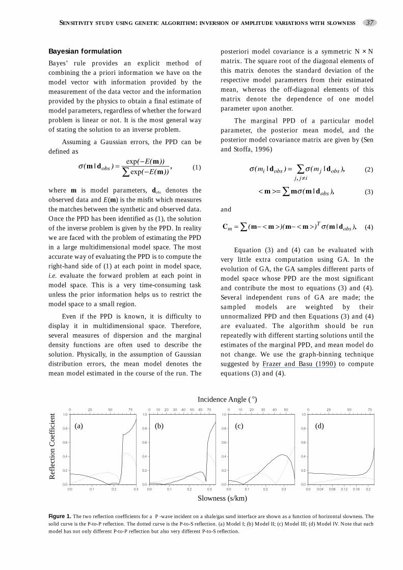
Figure 1. The two reflection coefficients for a P -wave incident on a shale/gas sand interface are shown as a function of horizontal slowness. Thesolid curve is the P-to-P reflection. The dotted curve is the P-to-S reflection. (a) Model I; (b) Model II; (c) Model III; (d) Model IV. Note that eachmodel has not only different P-to-P reflection but also very different P-to-S reflection.

Sensitivity analysis

Four two-layer models that represent the typicalrange of AVS responses associated with gas sandsnormally encountered in exploration are considered.Model I, II and III are the class I,II and III based onthe normal-incidence reflection coefficient(Rutherford and Williams 1989), and Model IV isthe class IV (Castagna et al., 1998). The parametersused for each model are shown in Table 1. Figure 1shows the absolute P-to-P and P-to-S reflectioncoefficients as functions of ray-parameter for eachtype of shale overlying gas sand model. We show theabsolute values of reflection coefficient because theybecome complex beyond critical angle, and thereforerequire a 3-D plot rather than 2-D shown here. Notethat the behavior of P-to-P and P-to-S reflectioncoefficients are complementary and should provideindependent information on the elastic parameters.

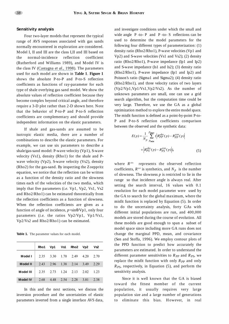
If shale and gas-sands are assumed to beisotropic elastic media, there are a number ofcombinations to describe the elastic parameters. Forexample, we can use six parameters to describe ashale/gas-sand model: P-wave velocity (Vp1), S-wavevelocity (Vs1), density (Rho1) for the shale and P-wave velocity (Vp2), S-wave velocity (Vs2), density(Rho2) for the gas-sand. By inspecting the Zoeppritzequation, we notice that the reflection can be writtenas a function of the density ratio and the slownesstimes each of the velocities of the two media, whichimply that five parameters (i.e. Vp1, Vp2, Vs1, Vs2and Rho2/Rho1) can be estimated theoretically fromthe reflection coefficients as a function of slowness.When the reflection coefficients are given as afunction of angle of incidence, p=sinθ/Vp1, only fourparameters (i.e. the ratios Vp2/Vp1, Vp1/Vs1,Vp2/Vs2 and Rho2/Rho1) can be estimated.

Table 1. The parameter values for each model.

In this and the next sections, we discuss theinversion procedure and the uncertainties of elasticparameters inverted from a single interface AVS data,

and investigate conditions under which the small andwide angle P -to- P and P -to- S reflections can beused to determine the model parameters for thefollowing four different types of parameterization: (1)density ratio (Rho2/Rho1), P-wave velocities (Vp1 andVp2) and S-wave velocities (Vs1 and Vs2); (2) densityratio (Rho2/Rho1), P-wave impedance (Ip1 and Ip2)and S-wave impedance (Is1 and Is2); (3) density ratio(Rho2/Rho1), P-wave impedance (Ip1 and Ip2) andPoisson’s ratio (Sigma1 and Sigma2); (4) density ratio(Rho2/Rho1), and three velocity ratios of two layers(Vp2/Vp1,Vp1/Vs1,Vp2/Vs2). As the number ofunknown parameters are small, one can use a gridsearch algorithm, but the computation time could bevery large. Therefore, we use the GA as a globaloptimization method to explore the entire model space.The misfit function is defined as a point-by-point P-to-P and P-to-S reflection coefficients comparisonbetween the observed and the synthetic data:

(5)

where Robs represents the observed reflectioncoefficients, Rsyn is synthetics, and Np is the numberof slowness. The slowness p is restricted to lie in therange so that incidence angle is always real. Aftersetting the search interval, 16 values with 0.1resolution for each model parameter were used bythe GA to search for the global maximum, where themisfit function is replaced by Equation (5). In orderto do the uncertainty analysis, forty GAs withdifferent initial populations are run, and 400,000models are stored during the course of evolution. Allthese models are good enough to span a subset ofmodel space since including more GA runs does notchange the marginal PPD, mean, and covariance(Sen and Stoffa, 1996). We employ contour plots ofthe PPD function to predict how accurately theparameters are estimated. In order to understand thedifferent parameter sensitivities to RPP and RPS, wereplace the misfit function with only RPP and onlyRPS, respectively, in Equation (5), and perform thesensitivity analysis.

Since it is well known that the GA is biasedtoward the fittest member of the currentpopulation, it usually requires very largepopulation size and a large number of generationsto eliminate this bias. However, in real

38 YING JI, SATISH SINGH & BRIAN HORNBY

Rho1 Vp1 Vs1 Rho2 Vp2 Vs2

Model I 2.35 3.30 1.70 2.49 4.20 2.70

Model II 2.43 2.96 1.38 2.14 3.49 2.29

Model III 2.35 2.73 1.24 2.13 2.02 1.23

Model IV 2.68 4.48 2.54 2.28 3.81 2.38

applications, the population size and the generationare usually limited. The PPD computed using thegraph-binning technique is biased by using these 40parallel GA runs even though each of them samplethe different most significant portions of the PPD.Therefore, in resolution analysis of contour plots ofthe PPD, we define an average marginal PPD,written as

i(6)to decrease the effects caused by the biased sampling,N(mi,mj) is the number of models when the modelparameters mi and mj are fixed.

Results

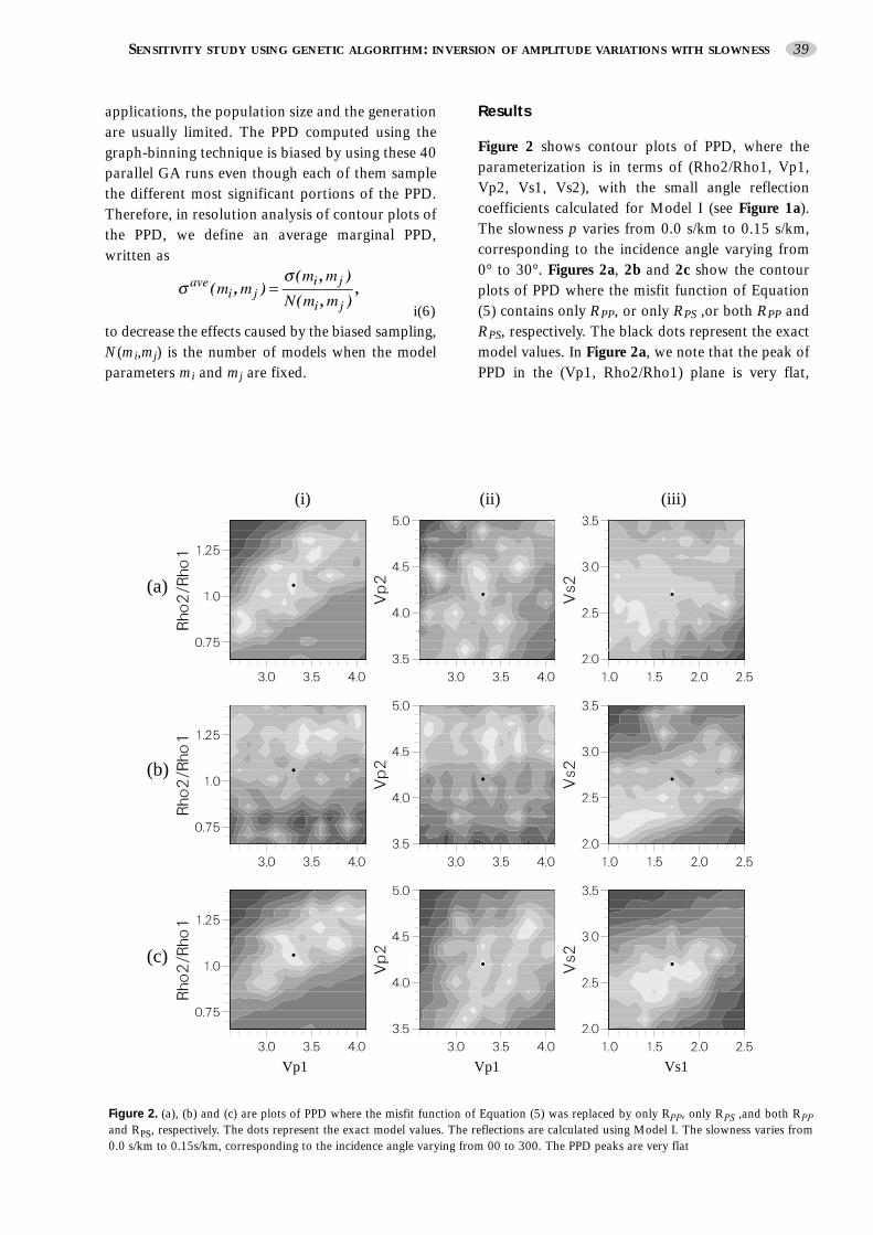
Figure 2 shows contour plots of PPD, where theparameterization is in terms of (Rho2/Rho1, Vp1,Vp2, Vs1, Vs2), with the small angle reflectioncoefficients calculated for Model I (see Figure 1a).The slowness p varies from 0.0 s/km to 0.15 s/km,corresponding to the incidence angle varying from0° to 30°. Figures 2a, 2b and 2c show the contourplots of PPD where the misfit function of Equation(5) contains only RPP, or only RPS ,or both RPP andRPS, respectively. The black dots represent the exactmodel values. In Figure 2a, we note that the peak ofPPD in the (Vp1, Rho2/Rho1) plane is very flat,

SENSITIVITY STUDY USING GENETIC ALGORITHM: INVERSION OF AMPLITUDE VARIATIONS WITH SLOWNESS 39

Vp1

(i)

Vs1

(c)

Vp1

(iii)(ii)

(b)

(a)

Figure 2. (a), (b) and (c) are plots of PPD where the misfit function of Equation (5) was replaced by only RPP, only RPS ,and both RPPand RPS, respectively. The dots represent the exact model values. The reflections are calculated using Model I. The slowness varies from0.0 s/km to 0.15s/km, corresponding to the incidence angle varying from 00 to 300. The PPD peaks are very flat

which indicates that small angle RPP reflectioncoefficient is not sensitive to the density ratioRho2/Rho1, and the existence of several secondarymaxima means that the ratio Rho2/Rho1 can not beinverted uniquely. The peaks in the velocity planesdistribute into a large part of model space. Thebroad width and several secondary maxima on thevelocity plots indicate that Vp1, Vp2 and Vs1 andVs2 can not be inverted uniquely. Figure 2bindicates that RPS is not sensitive to the P-wavevelocities. In Figure 2c, the plots in the(Vp1,Rho2/Rho1) plane and (Vp1, Vp2) plane showa similar pattern with those of Figure 2a, whichmeans that RPP is more sensitive to the density ratioRho2/Rho1 than RPS. The PPD peak in the(Vs1,Vs2) plane demonstrates a linear correlation,which suggests that a linear combination of Vs1 andVs2 is better estimated than the absolute values ofthem. The several secondary maxima are still

present in these plots, suggesting the miltimodalnature of the misfit function.

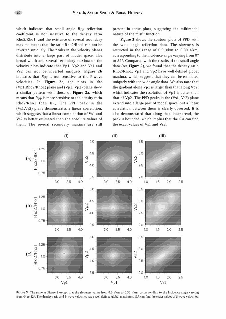
Figure 3 shows the contour plots of PPD withthe wide angle reflection data. The slowness isrestricted in the range of 0.0 s/km to 0.30 s/km,corresponding to the incidence angle varying from 0°to 82°. Compared with the results of the small angledata (see Figure 2), we found that the density ratioRho2/Rho1, Vp1 and Vp2 have well defined globalmaxima, which suggests that they can be estimateduniquely with the wide angle data. We also note thatthe gradient along Vp1 is larger than that along Vp2,which indicates the resolution of Vp1 is better thanthat of Vp2. The PPD peaks in the (Vs1, Vs2) planeextend into a large part of model space, but a linearcorrelation between them is clearly observed. It isalso demonstrated that along that linear trend, thepeak is bounded, which implies that the GA can findthe exact values of Vs1 and Vs2.

40 YING JI, SATISH SINGH & BRIAN HORNBY

Vp1

(i)

Vs1

(c)

Vp1

(iii)(ii)

(b)

(a)

Figure 3. The same as Figure 2 except that the slowness varies from 0.0 s/km to 0.30 s/km, corresponding to the incidence angle varyingfrom 0° to 82°. The density ratio and P-wave velocities has a well defined global maximum. GA can find the exact values of S-wave velocities.

SENSITIVITY STUDY USING GENETIC ALGORITHM: INVERSION OF AMPLITUDE VARIATIONS WITH SLOWNESS 41

From wide angle data sensitivity analysisresults, we infer that including wide angle data canimprove the resolution of inversion, and the wideangle RPP and RPS can invert the ratio Rho2/Rho1,Vp1, Vp2 and Vs1, Vs2 with high accuracy.

We performed the same sensitivity analysis onthe other three models with the small angle (less than30°) and the wide angle (up to 80°) data with thesame parameterization as the above. The followingresults are obtained:

Model II: Similar results are observed.

Model III: A secondary maximum is observed in the(Vp1,Rho2/Rho1) plane, and the peak has beenelongated along Rho2/Rho1 axis, which means thatresolution becomes worse, but the PPD is such thatthe GA can find the exact value of Rho2/Rho1 withthe wide-angle data. The linear correlation betweenVs1 and Vs2 is present, and the GA can not find the

absolute values of them.

Model IV: A secondary maximum and theelongation are also observed in the(Vp1,Rho2/Rho1) plane. The resolution of Vs1 andVs2 is better than Model III because the contrast islarger, but several secondary maxima appear.

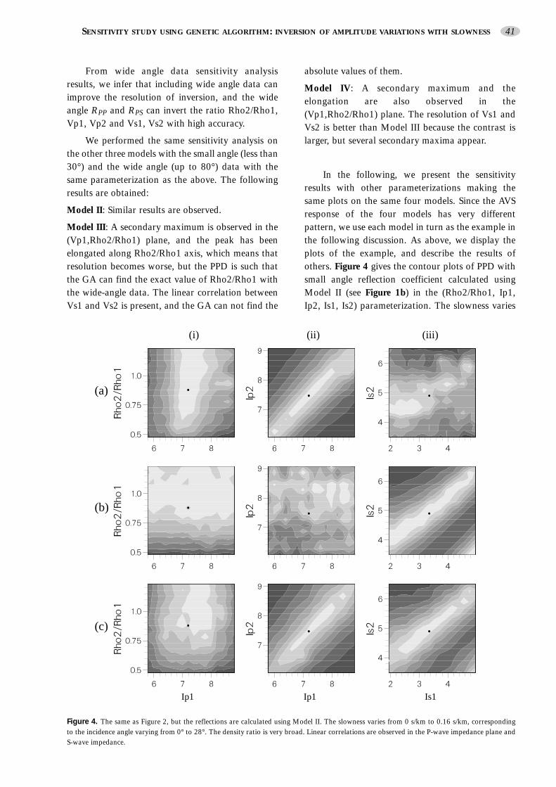
In the following, we present the sensitivityresults with other parameterizations making thesame plots on the same four models. Since the AVSresponse of the four models has very differentpattern, we use each model in turn as the example inthe following discussion. As above, we display theplots of the example, and describe the results ofothers. Figure 4 gives the contour plots of PPD withsmall angle reflection coefficient calculated usingModel II (see Figure 1b) in the (Rho2/Rho1, Ip1,Ip2, Is1, Is2) parameterization. The slowness varies

Ip1

(i)

Is1

(c)

Ip1

(iii)(ii)

(b)

(a)

Figure 4. The same as Figure 2, but the reflections are calculated using Model II. The slowness varies from 0 s/km to 0.16 s/km, correspondingto the incidence angle varying from 0° to 28°. The density ratio is very broad. Linear correlations are observed in the P-wave impedance plane andS-wave impedance.

42 YING JI, SATISH SINGH & BRIAN HORNBY

from 0.0 s/km to 0.16 s/km (incidence angle variesfrom 0° to 28°). The flat and broad peak of PPD inthe (Ip1, Rho2/Rho1) plane of Figure 4a suggeststhat the density ratio Rho2/Rho1 can not beestimated. The contour plots in the (Ip1, Ip2) planeshow very clear linear dependence between the P-wave impedance of the two layers. The convergencetendency toward the ratio of P-wave impedancesuggests that the ratio of the P-wave impedance oftwo layers can be estimated. Figure 4b gives the plotsof PPD using RPS. The same flat contour plots in thedensity ratio and the P-wave impedance planesuggest that RPS contains little information aboutthem. The contour plot of PPD in the S-waveimpedance plane shows a strong linear correlationbetween Is1 and Is2. The broad width of PPD alongthe linear correlation line indicates that the ratio ofS-wave impedance can be estimated. Figure 4c showsthe results using both RPP and RPS. The peak for

density ratio is very broad. The contour plot in theP-wave impedance plane has similar pattern to thatof Figure 4a, which implies RPS is not sensitive to theP-wave impedance. The plot in the S-waveimpedance plane indicates that a ratio of S-waveimpedance can be inverted with slightly betterresolution than Figure 4b.

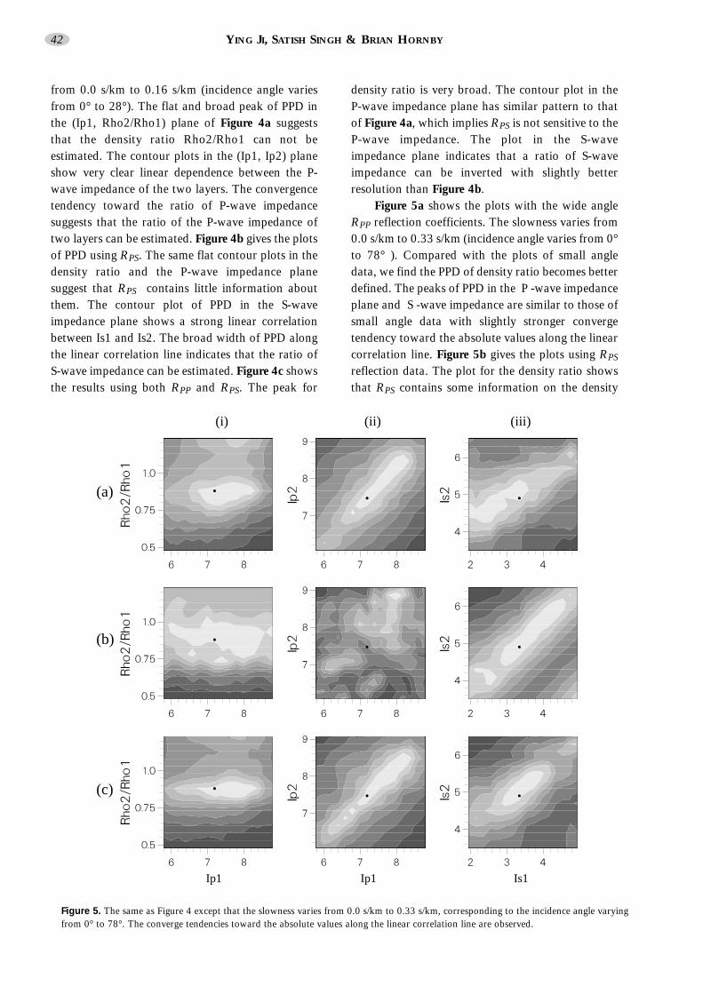
Figure 5a shows the plots with the wide angleRPP reflection coefficients. The slowness varies from0.0 s/km to 0.33 s/km (incidence angle varies from 0°to 78° ). Compared with the plots of small angledata, we find the PPD of density ratio becomes betterdefined. The peaks of PPD in the P -wave impedanceplane and S -wave impedance are similar to those ofsmall angle data with slightly stronger convergetendency toward the absolute values along the linearcorrelation line. Figure 5b gives the plots using RPS

reflection data. The plot for the density ratio showsthat RPS contains some information on the density

Ip1

(i)

Is1

(c)

Ip1

(iii)(ii)

(b)

(a)

Figure 5. The same as Figure 4 except that the slowness varies from 0.0 s/km to 0.33 s/km, corresponding to the incidence angle varyingfrom 0° to 78°. The converge tendencies toward the absolute values along the linear correlation line are observed.

SENSITIVITY STUDY USING GENETIC ALGORITHM: INVERSION OF AMPLITUDE VARIATIONS WITH SLOWNESS 43

ratio. The plot for P-wave impedance shows that itcontains little information about them. The plot inthe S-wave impedance plane has similar pattern withthat of small angle data, and a linear trend isobserved. Figure 5c gives the plots using both RPP

and RPS data. It is obvious that the density ratio canbe estimated. Similar patterns to Figure 5a in the P-wave impedance plane are observed since RPS is notsensitive to the P-wave impedance. The plot in the S-wave impedance plane obviously demonstratessignificant improvement in resolution of shear waveimpedance.

The results performed on the other models are:

Model I: Similar results are observed for the densityratio and P-wave impedance. The resolution of S-wave impedance is slightly worse.

Model III: The multiple and very broad width ofPPD peaks for the density ratio suggest that the

density ratio can not be estimated. Similar results forthe P-wave impedance with slightly better resolutionare observed. The S-wave impedance can not beestimated because of the low contrast.

Model IV: The density ratio estimation has greateruncertainty than that for Model II. Similar results forthe P-wave and S-wave impedance are observed.

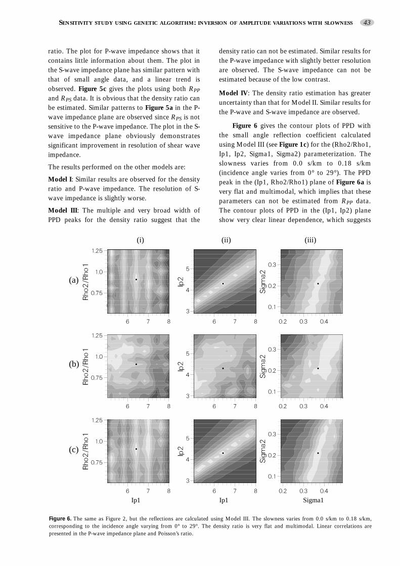
Figure 6 gives the contour plots of PPD withthe small angle reflection coefficient calculatedusing Model III (see Figure 1c) for the (Rho2/Rho1,Ip1, Ip2, Sigma1, Sigma2) parameterization. Theslowness varies from 0.0 s/km to 0.18 s/km(incidence angle varies from 0° to 29°). The PPDpeak in the (Ip1, Rho2/Rho1) plane of Figure 6a isvery flat and multimodal, which implies that theseparameters can not be estimated from RPP data.The contour plots of PPD in the (Ip1, Ip2) planeshow very clear linear dependence, which suggests

Ip1

(i)

Sigma1

(c)

Ip1

(iii)(ii)

(b)

(a)

Figure 6. The same as Figure 2, but the reflections are calculated using Model III. The slowness varies from 0.0 s/km to 0.18 s/km,corresponding to the incidence angle varying from 0° to 29°. The density ratio is very flat and multimodal. Linear correlations arepresented in the P-wave impedance plane and Poisson’s ratio.

that the ratio of Ip1 and Ip2 can be estimated.There is some linear correlation in the contourplots of the (Sigma1,Sigma2) plane. This indicatesthat Sigma1 and Sigma2 can only be estimated withlarge uncertainties. In Figure 6b, the flat peak in the(Rho2/Rho1, Ip1) plane suggests that RPS containslittle information about them. The contour plots inthe (Sigma1, Sigma2) plane show a linearcorrelation between them, but flat peaks of PPDindicate that they are difficult to estimate. Figure 6cshows the results using both RPP and RPS. The plotfor density ratio is similar to Figure 6a. Thecontour plot for the impedance clearlydemonstrates that the ratio of impedance of twolayers can be inverted. The plot in the (Sigma1,Sigma2) plane indicates that a combination ofSigma1 and Sigma2 can be inverted.

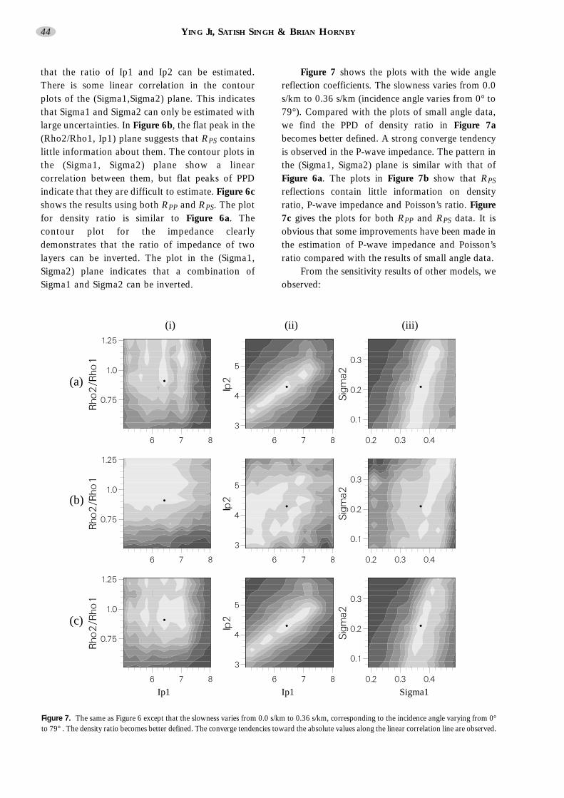
Figure 7 shows the plots with the wide anglereflection coefficients. The slowness varies from 0.0s/km to 0.36 s/km (incidence angle varies from 0° to79°). Compared with the plots of small angle data,we find the PPD of density ratio in Figure 7abecomes better defined. A strong converge tendencyis observed in the P-wave impedance. The pattern inthe (Sigma1, Sigma2) plane is similar with that ofFigure 6a. The plots in Figure 7b show that RPS

reflections contain little information on densityratio, P-wave impedance and Poisson’s ratio. Figure7c gives the plots for both RPP and RPS data. It isobvious that some improvements have been made inthe estimation of P-wave impedance and Poisson’sratio compared with the results of small angle data.

From the sensitivity results of other models, weobserved:

44 YING JI, SATISH SINGH & BRIAN HORNBY

Ip1

(i)

Sigma1

(c)

Ip1

(iii)(ii)

(b)

(a)

Figure 7. The same as Figure 6 except that the slowness varies from 0.0 s/km to 0.36 s/km, corresponding to the incidence angle varying from 0°to 79° . The density ratio becomes better defined. The converge tendencies toward the absolute values along the linear correlation line are observed.

Model I: The density ratio can be estimated withvery good resolution. The ratio of P-waveimpedance can be estimated. The absolute valuesof Poisson’s ratio can be found by GA.

Model II: The density ratio and the ratio ofimpedance can be well estimated. The absolutevalues of Poisson’s ratio can be found by GA.

Model IV: The density ratio is better estimatedthan Model III. Similar results for P-waveimpedance and Poisson’s ratio are obtained.

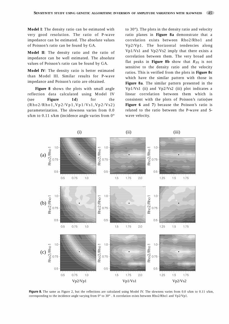
Figure 8 shows the plots with small anglereflection data calculated using Model IV (see Figure 1d) for the(Rho2/Rho1,Vp2/Vp1,Vp1/Vs1 ,Vp2/Vs2)parameterization. The slowness varies from 0.0s/km to 0.11 s/km (incidence angle varies from 0°

to 30°). The plots in the density ratio and velocityratio planes in Figure 8a demonstrate that acorrelation exists between Rho2/Rho1 andVp2/Vp1. The horizontal tendencies alongVp1/Vs1 and Vp2/Vs2 imply that there exists acorrelation between them. The very broad andflat peaks in Figure 8b show that RPS is notsensitive to the density ratio and the velocityratios. This is verified from the plots in Figure 8cwhich have the similar pattern with those inFigure 8a. The similar pattern presented in theVp1/Vs1 (ii) and Vp2/Vs2 (iii) plot indicates alinear correlation between them which isconsistent with the plots of Poisson’s ratio(seeFigure 6 and 7) because the Poisson’s ratio isrelated to the ratio between the P-wave and S-wave velocity.

SENSITIVITY STUDY USING GENETIC ALGORITHM: INVERSION OF AMPLITUDE VARIATIONS WITH SLOWNESS 45

Vp2/Vp1

(i)

(c)

Vp1/Vs1

(iii)(ii)

(b)

(a)

Vp2/Vs2

Figure 8. The same as Figure 2, but the reflections are calculated using Model IV. The slowness varies from 0.0 s/km to 0.11 s/km,corresponding to the incidence angle varying from 0° to 30° . A correlation exists between Rho2/Rho1 and Vp2/Vp1.

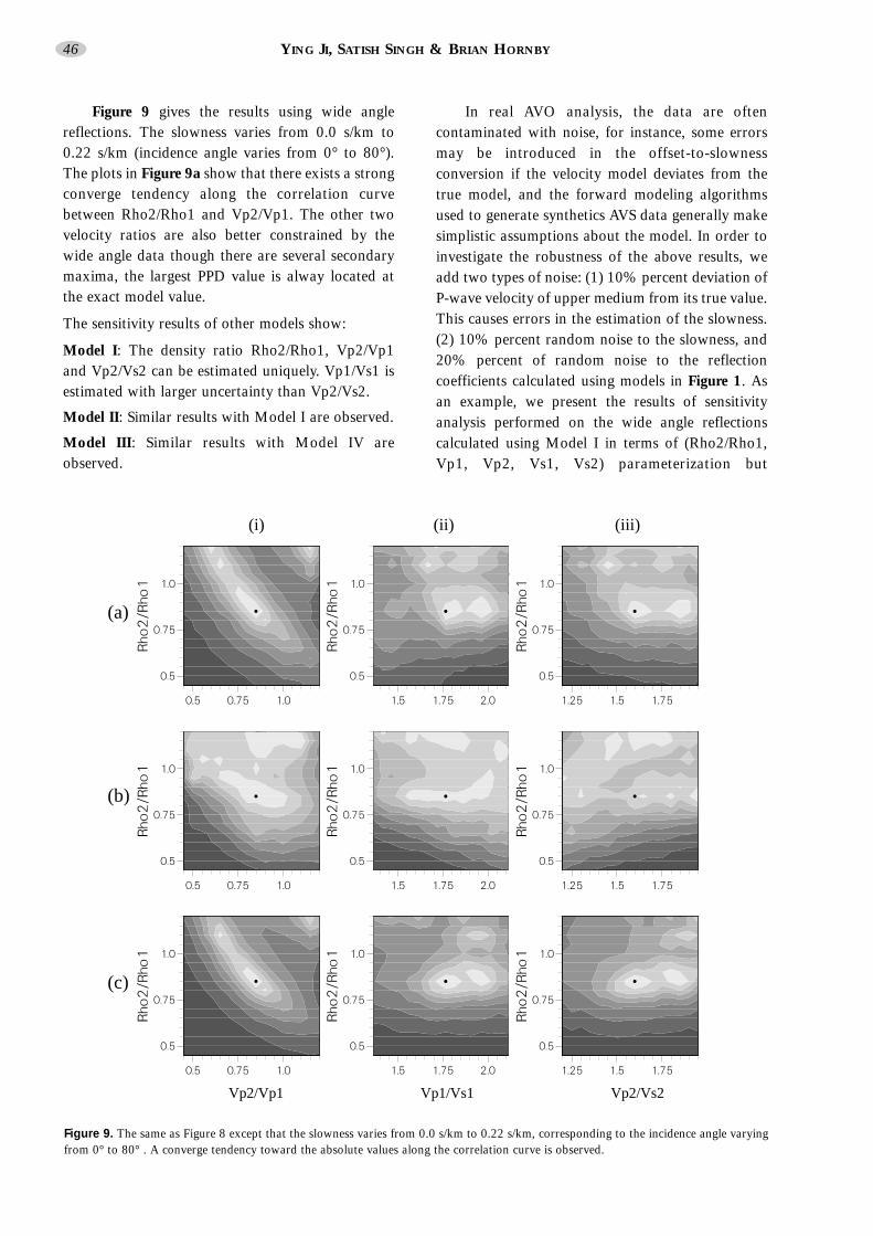
Figure 9 gives the results using wide anglereflections. The slowness varies from 0.0 s/km to0.22 s/km (incidence angle varies from 0° to 80°).The plots in Figure 9a show that there exists a strongconverge tendency along the correlation curvebetween Rho2/Rho1 and Vp2/Vp1. The other twovelocity ratios are also better constrained by thewide angle data though there are several secondarymaxima, the largest PPD value is alway located atthe exact model value.

The sensitivity results of other models show:

Model I: The density ratio Rho2/Rho1, Vp2/Vp1and Vp2/Vs2 can be estimated uniquely. Vp1/Vs1 isestimated with larger uncertainty than Vp2/Vs2.

Model II: Similar results with Model I are observed.

Model III: Similar results with Model IV areobserved.

In real AVO analysis, the data are oftencontaminated with noise, for instance, some errorsmay be introduced in the offset-to-slownessconversion if the velocity model deviates from thetrue model, and the forward modeling algorithmsused to generate synthetics AVS data generally makesimplistic assumptions about the model. In order toinvestigate the robustness of the above results, weadd two types of noise: (1) 10% percent deviation ofP-wave velocity of upper medium from its true value.This causes errors in the estimation of the slowness.(2) 10% percent random noise to the slowness, and20% percent of random noise to the reflectioncoefficients calculated using models in Figure 1. Asan example, we present the results of sensitivityanalysis performed on the wide angle reflectionscalculated using Model I in terms of (Rho2/Rho1,Vp1, Vp2, Vs1, Vs2) parameterization but

46 YING JI, SATISH SINGH & BRIAN HORNBY

Vp2/Vp1

(i)

(c)

Vp1/Vs1

(iii)(ii)

(b)

(a)

Vp2/Vs2

Figure 9. The same as Figure 8 except that the slowness varies from 0.0 s/km to 0.22 s/km, corresponding to the incidence angle varyingfrom 0° to 80° . A converge tendency toward the absolute values along the correlation curve is observed.

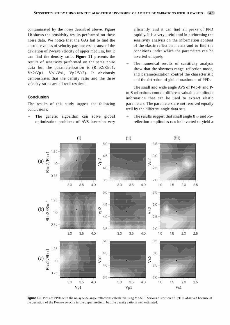
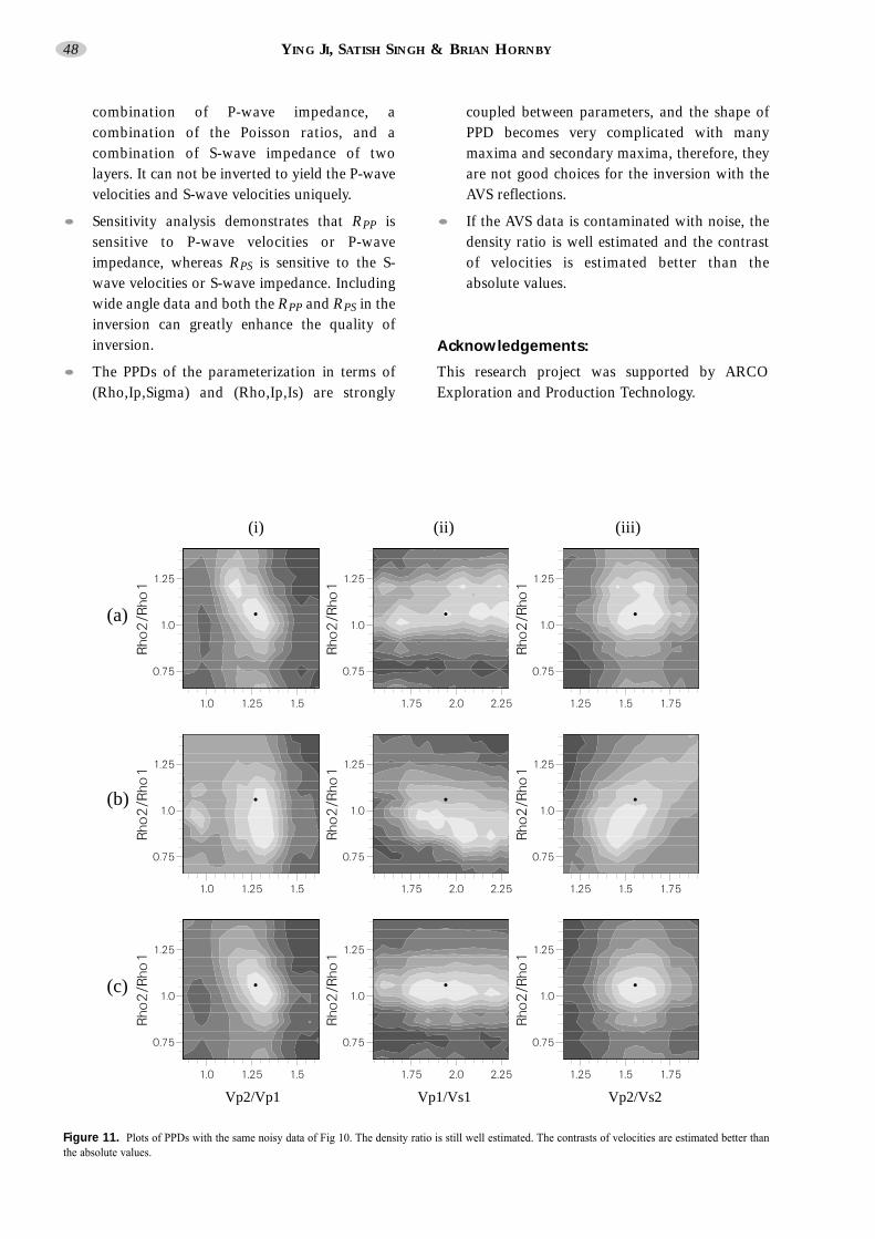
contaminated by the noise described above. Figure10 shows the sensitivity results performed on thesenoise data. We notice that the GAs fail to find theabsolute values of velocity parameters because of thedeviation of P-wave velocity of upper medium, but itcan find the density ratio. Figure 11 presents theresults of sensitivity performed on the same noisedata but the parameterization is (Rho2/Rho1,Vp2/Vp1, Vp1/Vs1, Vp2/Vs2). It obviouslydemonstrates that the density ratio and the threevelocity ratios are all well resolved.

Conclusion

The results of this study suggest the followingconclusions:

• The genetic algorithm can solve globaloptimization problems of AVS inversion very

efficiently, and it can find all peaks of PPDrapidly. It is a very useful tool in performing thesensitivity analysis on the information contentof the elastic reflection matrix and to find theconditions under which the parameters can beinverted uniquely.

• The numerical results of sensitivity analysisshow that the slowness range, reflection mode,and parameterization control the characteristicand the detection of global maximum of PPD.

The small and wide angle AVS of P-to-P and P-to-S reflections contain different valuable amplitudeinformation that can be used to extract elasticparameters. The parameters are not resolved equallywell by the different angle data sets.

• The results suggest that small angle RPP and RPS

reflection amplitudes can be inverted to yield a

SENSITIVITY STUDY USING GENETIC ALGORITHM: INVERSION OF AMPLITUDE VARIATIONS WITH SLOWNESS 47

Vp1

(i)

(c)

Vp1

(iii)(ii)

(b)

(a)

Vs1

Figure 10. Plots of PPDs with the noisy wide angle reflections calculated using Model I. Serious distortion of PPD is observed because ofthe deviation of the P-wave velocity in the upper medium, but the density ratio is well estimated.

combination of P-wave impedance, acombination of the Poisson ratios, and acombination of S-wave impedance of twolayers. It can not be inverted to yield the P-wavevelocities and S-wave velocities uniquely.

• Sensitivity analysis demonstrates that RPP issensitive to P-wave velocities or P-waveimpedance, whereas RPS is sensitive to the S-wave velocities or S-wave impedance. Includingwide angle data and both the RPP and RPS in theinversion can greatly enhance the quality ofinversion.

• The PPDs of the parameterization in terms of(Rho,Ip,Sigma) and (Rho,Ip,Is) are strongly

coupled between parameters, and the shape ofPPD becomes very complicated with manymaxima and secondary maxima, therefore, theyare not good choices for the inversion with theAVS reflections.

• If the AVS data is contaminated with noise, thedensity ratio is well estimated and the contrastof velocities is estimated better than theabsolute values.

Acknowledgements:

This research project was supported by ARCOExploration and Production Technology.

48 YING JI, SATISH SINGH & BRIAN HORNBY

Vp2/Vp1

(i)

Vp2/Vs2

(c)

Vp1/Vs1

(iii)(ii)

(b)

(a)

Figure 11. Plots of PPDs with the same noisy data of Fig 10. The density ratio is still well estimated. The contrasts of velocities are estimated better thanthe absolute values.

References

CASTAGNA J.P., SWAN H.W., AND FOSTER D.J., 1998.Framework for AVO gradient and interceptinterpretation. Geophysics, 63, 948-956.

DE HAAS J.C. AND BERKHOUT A.J., 1988. On theinformation content of P-P, P-SV, SV-SV, and SV-P reflections. 58th Annual InternationalMeeting., SEG, Expanded Abstracts, 1190-1194.

DI NICOLA A., DRUFICA G., AND ROCCA F., 1993.Eigenvalues and eigenvectors of linearized elasticinversion. Geophysics, 58, 670-679.

DU X. AND SPENCER T., 1990. Quantitative analysisof amplitude versus offset. 60th AnnualInternational Meeting., SEG, ExpandedAbstracts, 1459-1462.

FRAZER L.N. AND BASU A., 1990. Freeze-bathinversion. 60th Annual International Meeting.,SEG, Expanded Abstracts, 1123-1125.

GOLDBERG D.E. AND SEGREST P., 1987. FiniteMarkov chain analysis of genetic algorithm.Genetic algorithms and their applications,Proceedings of Second International Conferenceon Genetic Algorithm, 1-8.

GOLDBERG D.E., 1989., Genetic algorithms inSearch, Optimization and Machine Learning.Addison Wesley Publishing company.

HELGESEN J. AND LANDRO M., 1993. Estimation ofelastic parameters from AVO effects in the tau-p domain. Geophysical Prospecting, 41, 341-366.

HOLLARD J.H., 1975. Adaptation in Natural andArtificial Systems. University of Michigan Press,USA.

MALLICK S., 1995. Model-based inversion ofamplitude-variation-with-offset data using agenetic algorithm. Geophysics, 60, 939-954.

NEVES F.A. AND SINGH S.C., 1996. Sensitivity study ofseismic reflection/refraction data. GeophysicalJournal International, 126, 470-476.

OSTRANDER W.J., 1984. Plane-wave reflectioncoefficients for gas sands at nonnormal angles ofincidence. Geophysics, 49, 1637-1648.

RUTHERFORD R.S. AND WILLIAMS R.H., 1989.Amplitude-versus-offset variations in gas sands.Geophysics, 54, 680-688.

SEN M.K. AND STOFFA P.L., 1996. Bayesian inference,Gibbs’ sampler and uncertainty estimation ingeophysical inversion. Geophysical Prospecting,44, 313-350.

SHUEY R.T,. 1985. A simplication of the zoeppritzequations. Geophysics, 50, 609-614.

STOFFA P.L. AND SEN M.K., 1991. Nonlinearmultiparameter optimization using geneticalgorithm: Inversion of plane wave seismograms.Geophysics, 56, 1794-1810.

URSIN B. AND TJALAND E., 1992. Informationcontent of the elastic reflection matrix. 62ndAnnual International Meeting, SEG, ExpandedAbstracts, 796-799.

SENSITIVITY STUDY USING GENETIC ALGORITHM: INVERSION OF AMPLITUDE VARIATIONS WITH SLOWNESS 49