Section Based Hex-Cell Routing ALGORITHM (SBHCR)

International Journal of Computer Networks & Communications (IJCNC) Vol.7, No.1, January 2015

DOI : 10.5121/ijcnc.2015.7112 167

SECTION BASED HEX-CELL ROUTING ALGORITHM

(SBHCR)

Mohammad Qatawneh, Ahmad Alamoush and Ja'far Alqatawna

King Abdullah II School for Information Technology, The University of Jordan, Amman,

Jordan

ABSTRACT A Hex-Cell network topology can be constructed using units of hexagon cells. It has been introduced in the

literature as interconnection network suitable for large parallel computers, which can connect large

number of nodes with three links per node. Although this topology exhibits attractive characteristics such

as embeddability, symmetry, regularity, strong resilience, and simple routing, the previously suggested

routing algorithms suffer from the high number of logical operations and the need for readdressing of

nodes every time a new level is add to the network. This negatively impacts the performance of the network

as it increases the execution time of these algorithms. In this paper we propose an improved optimal point

to point routing algorithm for Hex-Cell network. The algorithm is based on dividing the Hex-Cell topology

into six divisions, hence the name Section Based Hex-Cell Routing (SBHCR). The SBHCR algorithm is

simple and preserves the advantage of the addressing scheme proposed for the Hex-Cell network. It does

not depend on the depth of the network topology which leads to overcome the issue of readdressing of

nodes every time a new level is added. Evaluation against two previously suggested routing algorithms has

shown the superiority of SBHCR in term of less logical operations.

KEYWORDS Hex-Cell topology, Routing Algorithm, Interconnection Topology, Networking.

1.INTRODUCTION

Routing algorithms is a popular topic in the study of computer networks, distributed systems and

their applications [1,2]. The design of routing algorithm plays an important role in determining

the performance of tightly and loosely coupled systems. The efficiency of many applications that

run on tightly and loosely coupled systems depends highly on communication time which is

affected by characteristics of routing algorithm. Routing algorithm should prove correctness,

simplicity, robustness, stability, fairness and optimality [3,4,5,6].

Several static interconnection networks and their related routing algorithms have been reported in

the literature [6,7,8,9,10]. Hex-Cell network is a class of interconnection networks which has

proposed for parallel computing systems [10,11,12,13,14]. Its topology can be constructed using

units of hexagon cells. Sharieh et al. [10] suggested the original routing algorithm in which the

addressing mode was based on the depth of the network and the position of the node in the level.

The routing from one node to another can be done using one or more of the following three

functions: moveUp, moveDown and moveHorizontal. Qatawneh et al. [11] have criticized the

dependency on the depth of Hex-Cell network which mean that the topology must be fixed

otherwise the depth value must be updated to readdress the nodes every time a new level is added.


168

Therefore, they have proposed an alternative routing algorithm in which the node addressing is

based on the address of the three cells around the node while the cell itself is addressed based on

Cartesian coordinate (X-axis and Y-axis). Their algorithm assumes the central cell is having (0,0)

as coordinate and in order to reach the destination two functions need to be used: Cell Routing

and Node Routing.

Although Hex-Cell topology exhibits attractive characteristics such as embeddability, symmetry,

regularity, strong resilience, and simplicity[10,11,12,13], the previously suggested routing

algorithms[10,11] suffer from the high number of logical operations and the need for readdressing

network nodes every time a new level is added which negatively impact the running time of that

network. Therefore, the aim of this paper is to propose a new routing algorithm for Hex-Cell

network that eliminate these shortcomings.

The rest of the paper is organized as follows. Section 2 provides an overview of Hex-Cell

network. Section 3 presents the proposed routing algorithm. Section 4 compares the algorithm to

its predecessor. Finally conclusion is presented in section 5.

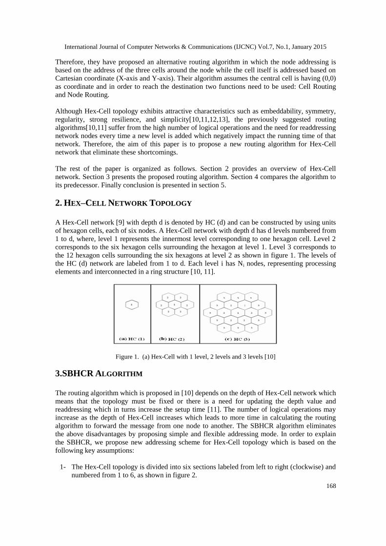
2. HEX–CELL NETWORK TOPOLOGY

A Hex-Cell network [9] with depth d is denoted by HC (d) and can be constructed by using units

of hexagon cells, each of six nodes. A Hex-Cell network with depth d has d levels numbered from

1 to d, where, level 1 represents the innermost level corresponding to one hexagon cell. Level 2

corresponds to the six hexagon cells surrounding the hexagon at level 1. Level 3 corresponds to

the 12 hexagon cells surrounding the six hexagons at level 2 as shown in figure 1. The levels of

the HC (d) network are labeled from 1 to d. Each level i has Ni nodes, representing processing

elements and interconnected in a ring structure [10, 11].

Figure 1. (a) Hex-Cell with 1 level, 2 levels and 3 levels [10]

3.SBHCR ALGORITHM

The routing algorithm which is proposed in [10] depends on the depth of Hex-Cell network which

means that the topology must be fixed or there is a need for updating the depth value and

readdressing which in turns increase the setup time [11]. The number of logical operations may

increase as the depth of Hex-Cell increases which leads to more time in calculating the routing

algorithm to forward the message from one node to another. The SBHCR algorithm eliminates

the above disadvantages by proposing simple and flexible addressing mode. In order to explain

the SBHCR, we propose new addressing scheme for Hex-Cell topology which is based on the

following key assumptions:

1- The Hex-Cell topology is divided into six sections labeled from left to right (clockwise) and

numbered from 1 to 6, as shown in figure 2.


169

2- The address of each node in the Hex-Cell topology is identified by (S,L,X) where S denotes

the section number, L denotes the level number, and X denotes the node number on that

level labeled from X1,…, Xn; where n = ((2×L) - 1).

Figure 2. Hex-Cell addressing scheme for HC (3) network

A node with the address 1.1.1 is the first node that exists at the section number 1 and level

number 1. A node 1.2.1 refers to first node that exists at the section number 1 and level number 2

and so on. In SBHCR algorithm for HC as shown in Figure 3, the movement from one node to

another can be done using one of the following five cases as shown in figure 3 (a).

Figure 3.(a) The main function for the SBHCR algorithm

As an input to this routing algorithm the address of the source node (which is the first node

address) and the address of the destination node (Ssrc, Lsrc, Xsrc, Sdest, Ldest, Xdest) is used to

get the output which is the address of the second node and the address of the destination node

(Snxt, Lnxt, Xnxt, Sdest, Ldest, Xdest). Then the second node apply the routing algorithm using

the address of the source node (which is the second node address in this case) and the address of

the destination node (Ssrc, Lsrc, Xsrc, Sdest, Ldest, Xdest) to get the address of the third node


170

and the address of the destination node (Snxt, Lnxt, Xnxt, Sdest, Ldest, Xdest). We continue this

way until we reach the source address equal the destination address.

moveToUpperLevelC1(Ssrc, Lsrc, Xsrc, Sdest, Ldest, Xdest)

Output(Snxt, Lnxt, Xnxt, Sdest, Ldest, Xdest) {

If (Lsrc is odd) return (Ssrc, Lsrc + 1, Xsrc + 1, Sdest, Ldest, Xdest)

Else

If (Xsrc < Xdest) return (Ssrc, Lsrc, Xsrc + 1, Sdest, Ldest, Xdest) Else return (Ssrc, Lsrc, Xsrc - 1, Sdest, Ldest, Xdest) }

---------------------------------------------------------------------------------------------------------------------

moveToLowerLevelC1(Ssrc, Lsrc, Xsrc, Sdest, Ldest, Xdest)

Output(Snxt, Lnxt, Xnxt, Sdest, Ldest, Xdest){

If (Lsrc is even) return (Ssrc, Lsrc - 1, Xsrc - 1, Sdest, Ldest, Xdest)

Else

If (Xsrc ≤ Xdest) return (Ssrc, Lsrc, Xsrc + 1, Sdest, Ldest, Xdest) Else return (Ssrc, Lsrc, Xsrc - 1, Sdest, Ldest, Xdest) }

---------------------------------------------------------------------------------------------------------------------



If (Xsrc is even) return (Ssrc, Lsrc - 1, Xsrc - 1, Sdest, Ldest, Xdest)

Else

If (Xsrc + 1 > ((2 × Lsrc) – 1))

If (Ssrc = 6) return(1, Lsrc, 1, Sdest, Ldest, Xdest) Else return (Ssrc + 1, Lsrc, 1, Sdest, Ldest, Xdest)

Else return (Ssrc, Lsrc, Xsrc + 1, Sdest, Ldest, Xdest)}

---------------------------------------------------------------------------------------------------------------------



If (Xsrc is even) return(Ssrc, Lsrc - 1, Xsrc - 1, Sdest, Ldest, Xdest)

Else

If (Xsrc + 1 > ((2 × Lsrc) – 1)) If (Ssrc = 6) return(1, Lsrc, 1, Sdest, Ldest, Xdest)

Else return (Ssrc + 1, Lsrc, 1, Sdest, Ldest, Xdest)


---------------------------------------------------------------------------------------------------------------------



If (Xsrc is even) return(Ssrc, Lsrc - 1, Xsrc - 1, Sdest, Ldest, Xdest) Else

If (Xsrc - 1 < 1)

If (Ssrc = 1) return (6, Lsrc, ((2 × Lsrc) – 1), Sdest, Ldest, Xdest)

Else return (Ssrc - 1, Lsrc, ((2 × Lsrc ) – 1), Sdest, Ldest, Xdest)

Else return (Ssrc, Lsrc, Xsrc - 1, Sdest, Ldest, Xdest) }

---------------------------------------------------------------------------------------------------------------------


Output(Snxt, Lnxt, Xnxt, Sdest, Ldest, Xdest){ If (Xsrc is even) return(Ssrc, Lsrc - 1, Xsrc - 1, Sdest, Ldest, Xdest)

Else

If (Xsrc - 1 < 1)

If (Ssrc = 1) return (6, Lsrc, ((2 × Lsrc) – 1), Sdest, Ldest, Xdest)

Else return (Ssrc - 1, Lsrc, ((2 × Lsrc ) – 1), Sdest, Ldest, Xdest)

Else return (Ssrc, Lsrc, Xsrc - 1, Sdest, Ldest, Xdest) }

---------------------------------------------------------------------------------------------------------------------

moveSameLevelC1(Ssrc, Lsrc, Xsrc, Sdest, Ldest, Xdest) Output(Snxt, Lnxt, Xnxt, Sdest, Ldest, Xdest){

If (Xsrc < Xdest) return (Ssrc, Lsrc, Xsrc + 1, Sdest, Ldest, Xdest)

Else return (Ssrc, Lsrc, Xsrc - 1, Sdest, Ldest, Xdest)}

---------------------------------------------------------------------------------------------------------------------

moveSameLevelC2(Ssrc, Lsrc, Xsrc, Sdest, Ldest, Xdest)


If (Xsrc + 1 > ((2 × Lsrc) – 1)) If (Ssrc = 6) return(1, Lsrc, 1, Sdest, Ldest, Xdest)

Else return (Ssrc + 1, Lsrc, 1, Sdest, Ldest, Xdest)


---------------------------------------------------------------------------------------------------------------------

moveSameLevelC5(Ssrc, Lsrc, Xsrc, Sdest, Ldest, Xdest)


If (Xsrc - 1 < 1)

If (Ssrc = 1) return (6, Lsrc, ((2 × Lsrc) – 1), Sdest, Ldest, Xdest) Else return (Ssrc - 1, Lsrc, ((2 × Lsrc ) – 1), Sdest, Ldest, Xdest)

Else return (Ssrc, Lsrc, Xsrc - 1, Sdest, Ldest, Xdest)}

Figure 3.(b) The sub-functions the SBHCR algorithm


171

4.SCENARIO BASED DISCUSSION

The following examples explain the above routing cases. For this purposed, we consider a

network of a Hex-cell topology with 4 levels; i.e. HC (4) as shown in Figure 4.

Figure 4. HC (4) topology with labeled nodes and levels

Scenario 1: The source and destination in the same section and level

Let (Ss.Ls.Xs) = (2.4.2) be the source node and (Sd.Ld.Xd) = (2.4.7) be the destination node. When

executing the routing algorithm, CASE 1 will be applied. To reach the destination, the algorithm

goes through five steps; i.e., (2.4.2) → (2.4.3) → (2.4.4) → (2.4.5) → (2.4.6) → (2.4.7) , as

shown in Figure (5).

Figure 5. The source and destination in the same section and level

Scenario 2: source and destination are in the same section and different levels

(destination level less than source level)


172

Let (Ss.Ls.Xs) = (5.4.5) be the source node and (Sd.Ld.Xd) = (5.2.1) be the destination node.

When executing the routing algorithm, CASE 1 will be applied. To reach the destination, the

algorithm goes through four steps; i.e., (5.4.5) → (5.4.4) → (5.3.3) → (5.3.2) → (5.2.1), as shown

in Figure (6).

Figure 6: source and destination are in the same section and different levels

(destination level less than source level).

Scenario 3: source and destination are in the same section and different levels

(source level less than destination level)



algorithm goes through five steps; i.e., (5.3.2) → (5.3.3) → (5.4.4) → (5.4.5) → (5.4.6) →

(5.4.7), as shown in Figure (7).

figure 7. Source and destination are in the same section and different levels

(source level less than destination level)

Scenario 4: source and destination are in different sections (Ss = Sd - 1 or Ss = Sd + 5)

(source level less than or equal destination level)


173



algorithm goes through six steps; i.e., (1.3.2) → (1.3.3) → (1.3.4) → (1.3.5) → (2.3.1) → (2.4.2)

→ (2.4.1), as shown in Figure (8).

Figure 8. Source and destination are in different sections (Ss = Sd - 1 or Ss = Sd + 5)

(source level less than or equal destination level).

Scenario 5: source and destination are in different sections (Ss = Sd - 1 or Ss = Sd +

5) (destination level less than source level)



algorithm goes through six steps; i.e., (1.4.4) → (1.3.3) → (1.3.4) → (1.2.3) → (2.2.1) → (2.2.2)

→ (2.2.3), as shown in Figure (9).

Figure 9. Source and destination are in different sections (Ss = Sd - 1 or Ss = Sd + 5)


Scenario 6: source and destination are in different sections (Ss = Sd – 2 or Ss = Sd + 4)




174

algorithm goes through nine steps; i.e., (4.3.2) → (4.2.1) → (4.2.2) → (4.1.1) → (5.1.1) → (6.1.1)

→ (6.2.2) → (6.2.3) → (6.3.4) → (6.3.3), as shown in Figure (10).

Figure 10. Source and destination are in the different sections (Ss = Sd - 2 or Ss = Sd + 4)

Scenario 7: source and destination are in different sections (Ss = Sd - 3 or Ss = Sd + 3

or Ss = Sd - 4 or Ss = Sd + 2 )



goes through eleven steps; i.e., (6.3.3) → (6.3.4) → (6.2.3) → (1.2.1) → (1.2.2) → (1.1.1) →

(2.1.1) → (3.1.1) → (3.2.2) → (3.2.3) → (3.3.4) → (3.3.3), as shown in Figure(11).

Figure 11. Source and destination are in different sections

(Ss = Sd - 3 or Ss = Sd + 3 or Ss = Sd - 4 or Ss = Sd + 2 )

Scenario 8: source and destination are in the different sections (Ss = Sd - 5 or Ss = Sd

+ 1) (source level less than or equal destination level).



goes through eight steps; i.e., (5.2.3) → (5.2.2) → (5.2.1) → (4.2.3) → (4.3.4) → (4.3.3) →

(4.4.4) → (4.4.3) → (4.4.2), as shown in Figure (12).


175

Figure 12. Source and destination are in the different sections (Ss = Sd - 5 or Ss = Sd + 1)

(source level less than or equal destination level).

Scenario 9: source and destination are in different sections (Ss = Sd - 5 or Ss = Sd + 1)




goes through five steps; i.e., (5.4.4) → (5.3.3) → (5.3.2) → (5.2.1) → (4.2.3) → (4.2.2), as shown

in Figure (13).

Figure 13. source and destination are in different sections (Ss = Sd - 5 or Ss = Sd + 1)


5.COMPARISON BETWEEN SBHCR AND OTHERS ALGORITHMS The original Hex-Cell routing [10] uses a centralized algorithm to find the best path from the

source to the destination. This means that one node do the job, and it is same in the alternative

algorithm proposed in [11]. In the contrary, in the SBHCR each node finds the best next node in

order to get to the final destination. Thus, the total number of required operation to perform


176

logical comparison is divided on the nodes, which would give better performance when compared

with a single node performing the same logical operation.

Table 1. Comparison between SBHCR and others algorithms.

For instance, the number of steps and logical comparison between two same nodes:

1) Original routing algorithm [10]:

a) From node (4.8) to (5.8) it takes 3 Steps and need 13 Logical Operations

b) From node (3.7) to (6.7) it takes 5 Steps and need 21 Logical Operations

2) Alternative Routing Algorithm [11]:

a) From node ((1,-1),(0,0),(1,1)) to ((-1,-1),(0,0),(-1,1)) it takes 3 Steps and

need 25 Logical Operations

b) From node ((1,-1),(2,0),(1,1)) to ((-1,-1),(-2,0),(-1,1))it takes 5 Steps and

need 85 Logical Operations

3) SBHCR Algorithm

a) From node (2.1.1) to (5.1.1) it takes 3 Steps and need 22 Logical

Operations

b) From node (2.2.2) to (5.2.2) it takes 5 Steps and need 32 Logical

Operations.

6.CONCLUSION

In this paper we propose a new routing algorithm for Hex-Cell network that eliminates the

weaknesses of the previously suggested algorithms. The algorithm is based on dividing the Hex-

Cell topology into six divisions and called Section Based Hex-Cell Routing (SBHCR). The

SBHCR algorithm is simple and preserves the advantage of the addressing scheme proposed for

the Hex-Cell network. The SBHCR does not depend on the depth like the current addressing

which means that the network can be extended without reconfiguration the whole network.

Moreover, in this algorithm the task of finding the best routing path is performed by more than

one node which implies better performance.

Proposed

Routing

Algorithm

Routing Algorithm in [11] Original Routing

Algorithm [10] First Cell Level

3 3 3 Number of Steps

23 25 13 Number of Logical Operations

sum, sub and

mod sum and sub sum, sub and mod Arithmetic operation

Second Cell Level

5 5 5 Number of Steps

32 85 21 Number of Logical Operations

sum, sub and

mod sum and sub sum, sub and mod Arithmetic operation


177

REFERENCES

[1] A

[2] Chatterjee, Pushpita. "Trust based

-

[3] Decayeux, Catherine, and David Seme. "3D hexagonal network: Modeling, topological properties,

addressing scheme, and optimal routing algorithm." Parallel and Distributed Systems, IEEE

Transactions on 16.9 (2005): 875-884.

[4] Tse-Yun Feng; Seung-Woo Seo, "A new routing algorithm for a class of rearrangeable networks,"

Computers, IEEE Transactions on , vol.43, no.11, pp.1270,1280, Nov 1994 doi: 10.1109/12.324560.

[5 ]Chen, Chi-Chang, and Jianer Chen. "Nearly optimal one-to-many parallel routing in star networks."

Parallel and Distributed Systems, IEEE Transactions on 8.12 (1997): 1196-1202.

[6] Mohammad, Qatawneh. "Adaptive fault tolerant routing algorithm for Tree-Hypercube

multicomputer." Journal of Computer Science 2, no. 2 (2006): 124.

[7] Li, Keqin. "Parallel processing of divisible loads on partitionable static interconnection networks."

Cluster Computing 6, no. 1 (2003): 47-55.

[8] Dündar, Pinar. "Stability measures of some static interconnection networks." International journal of

computer mathematics 76, no. 4 (2001): 455-462.

[9] Abd-El-Barr, Mostafa, and Fayez Gebali. "Reliability analysis and fault tolerance for hypercube

multi-computer networks." Information Sciences 276 (2014): 295-318.

[10] Ahmad Sharieh, Mohammad Qatawneh, Wesam Almobaideen, Azzam Sleit, Hex-Cell: Modeling,

Topological Properties and Routing Algorithm, European Journal of Scientific Research, 22:2(2008),

457-468.

[11] Mohammad Qatawneh, Hamed Bdour, Shrouq Sabah, Rana Samhan, Azzam sliet, Ja'far Alqatawna,

Wesam al-Mobaideen. An alternative Routing Algorithm for Hex-Cell network. Information: An

International. Information: an international interdisciplinary journal. 14(10). Pp.3499-3514. 2011.

[12] Mohammad Qatawneh, Embedding Binary Tree and Bus into Hex-Cell Interconnection Network.

Journal of American Science, 2011; 7(12).

[13] Mohammad Qatawneh, Bdour Hamed, Wesam AlMobaideen, Azzam Sleit, Amal Oudat, Wala’a

Qutechat, Roba Al-Soub, FTRH: Fault-Tolerance Routing Algorithm for Hex-Cell Network. IJCSNS

International Journal of Computer Science and Network Security, VOL.9 No.12, December 2009.

[14] Mohammad Qatawneh, Multilayer Hex-Cells: A New Class of Hex-Cell Interconnection Networks

for Massively parallel Systems. Int. J. Communications, Network and System Sciences, 4(11) 2011.

Section Based Hex-Cell Routing ALGORITHM (SBHCR)

Documents

Transcript of Section Based Hex-Cell Routing ALGORITHM (SBHCR)